time series analysis: 1. sampling and dft

Time Series Analysis:

1. Sampling and DFT

P. F. Górahttp://th-www.if.uj.edu.pl/zfs/gora/

2012

http://th-www.if.uj.edu.pl/zfs/gora/

The rules

6–7 written assignments (numerical and theoretical)

• All assignments done — ,

• Half or more assignments done — an exam

• Less than half assignments done — /

All assignments will be published on my webpage

Copyright c© 2009-12 P. F. Góra 1–2

The objective

Given a time series

xiNi=1 = x1, x2, . . . , xN

(usually boring), gain some insight on the mechanism that is responsible forgenerating this series (possibly interesting).


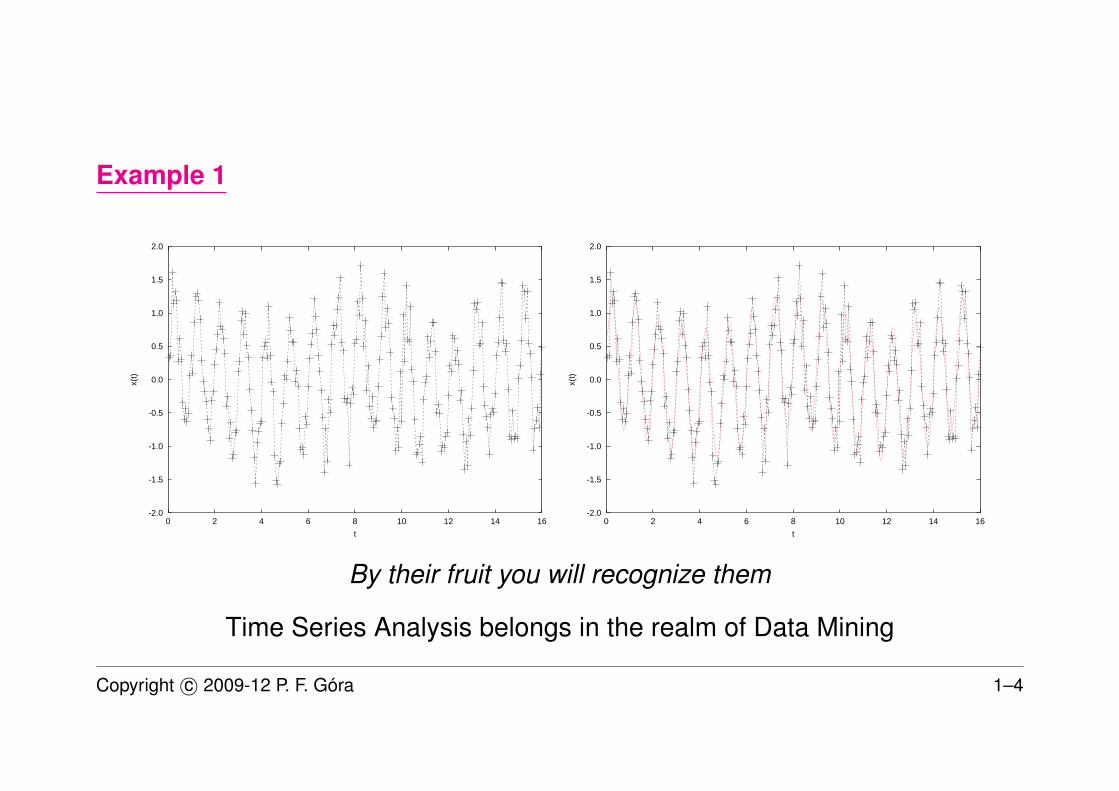
Example 1

-2.0

-1.5

-1.0

-0.5

0.0

0.5

1.0

1.5

2.0

0 2 4 6 8 10 12 14 16

x(t)

t

-2.0

-1.5

-1.0

-0.5

0.0

0.5

1.0

1.5

2.0

0 2 4 6 8 10 12 14 16

x(t)

t

By their fruit you will recognize them

Time Series Analysis belongs in the realm of Data Mining


The plan∗

1. Introduction; Sampling and Discrete Fourier Transform; a Fast Fourier Transform Algorithm2. Convolution, stationarity, Power Spectrum and windowing functions; Wiener filter3. Linear filters4. Stationary linear stochastic models (AR, MA, ARMA)5. Fitting parameters to stationary linear stochastic models; Youle-Walker equations; Akaike criterion; Linear

prediction6. Seasonal changes and trends (ARIMA)7. Models with time-varying parameters of noise8. Principal Components Analysis9. Wavelets

10. Applications of wavelets11. Hurst phenomenon, fractional processes and Detrended Fluctuations Analysis12. Kalman filters13. Takens theorem and phase space reconstruction14. Applications of Takens theorem

∗May change dynamically!


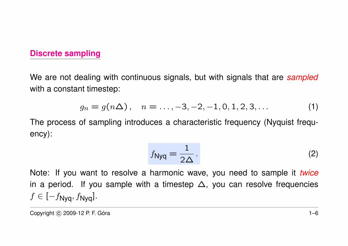
Discrete sampling

We are not dealing with continuous signals, but with signals that are sampledwith a constant timestep:

gn = g(n∆) , n = . . . ,−3,−2,−1,0,1,2,3, . . . (1)

The process of sampling introduces a characteristic frequency (Nyquist frequ-ency):

fNyq =1

2∆. (2)

Note: If you want to resolve a harmonic wave, you need to sample it twicein a period. If you sample with a timestep ∆, you can resolve frequenciesf ∈ [−fNyq, fNyq].


Positive and negative frequencies

If you allow for both positive and negative frequencies, e+2πift, e−2πift =

e+2πi(−f)t, you can combine them to get both sin 2πft and cos 2πft, whichhave the same frequency , but differ in phase.


Shannon-Kotelnikov Sampling Theorem

Question: When can we sample? Or, under what assumptions discrete samplingyields the same information as a continuous function?

Theorem: If a function g(t) is bandwidth limited , or if it contains only frequenciesfrom the interval [−fNyq, fNyq], and if we have an infinite series sampled with atimestep ∆, then

∀t : g(t) = ∆∞∑

n=−∞gn

sin(2πfNyq(t− n∆)

)π(t− n∆)

. (3)

Noise (stochastic processes) and not continuous functions are not bandwidthlimited.Copyright c© 2009-12 P. F. Góra 1–8

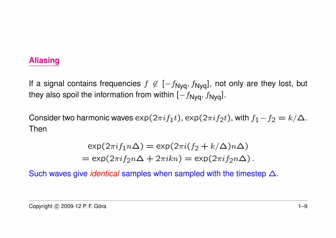
Aliasing

If a signal contains frequencies f 6∈ [−fNyq, fNyq], not only are they lost, butthey also spoil the information from within [−fNyq, fNyq].

Consider two harmonic waves exp(2πif1t), exp(2πif2t), with f1−f2 = k/∆.Then

exp(2πif1n∆) = exp(2πi(f2 + k/∆)n∆)

= exp(2πif2n∆ + 2πikn) = exp(2πif2n∆) .

Such waves give identical samples when sampled with the timestep ∆.


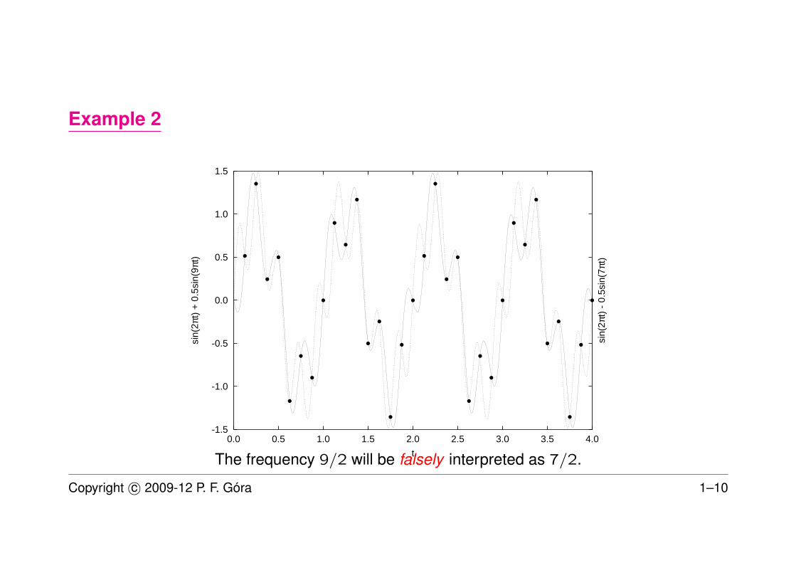
Example 2

-1.5

-1.0

-0.5

0.0

0.5

1.0

1.5

0.0 0.5 1.0 1.5 2.0 2.5 3.0 3.5 4.0

sin(

2πt)

+ 0

.5si

n(9π

t)

sin(

2πt)

- 0

.5si

n(7π

t)

tThe frequency 9/2 will be falsely interpreted as 7/2.


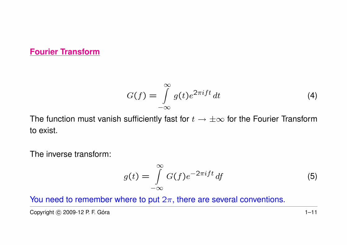
Fourier Transform

G(f) =

∞∫−∞

g(t)e2πift dt (4)

The function must vanish sufficiently fast for t → ±∞ for the Fourier Transformto exist.

The inverse transform:

g(t) =

∞∫−∞

G(f)e−2πift df (5)

You need to remember where to put 2π, there are several conventions.Copyright c© 2009-12 P. F. Góra 1–11

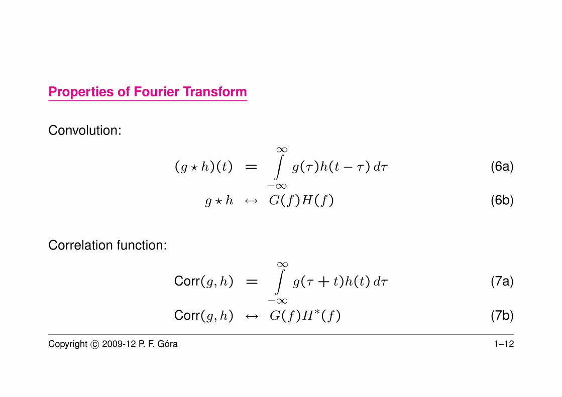
Properties of Fourier Transform

Convolution:

(g ? h)(t) =

∞∫−∞

g(τ)h(t− τ) dτ (6a)

g ? h ↔ G(f)H(f) (6b)

Correlation function:

Corr(g, h) =

∞∫−∞

g(τ + t)h(t) dτ (7a)

Corr(g, h) ↔ G(f)H∗(f) (7b)


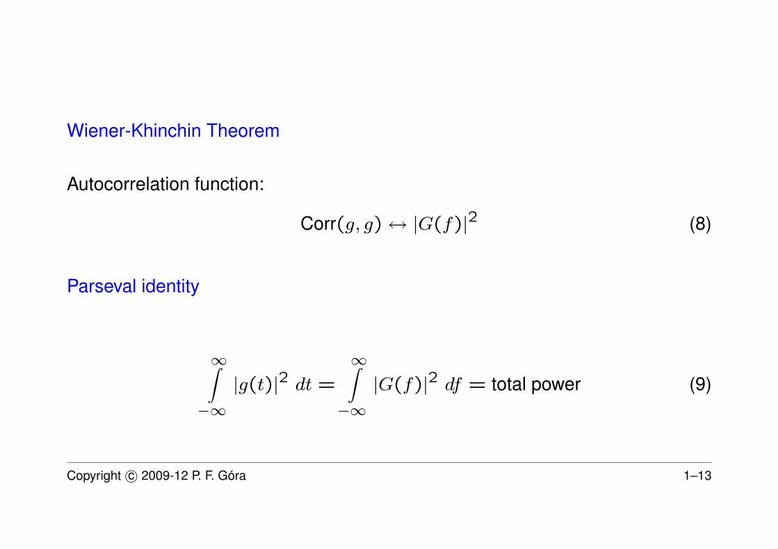
Wiener-Khinchin Theorem

Autocorrelation function:

Corr(g, g)↔ |G(f)|2 (8)

Parseval identity

∞∫−∞|g(t)|2 dt =

∞∫−∞|G(f)|2 df = total power (9)


Finite time series

The sampling theorem requires an infinite series, but in reality we only havea finite series, of the length N . There are two conventions

• We assume that the series goes to zero at both its ends (we multiply byan appropriate windowing function if it doesn’t) and equals identically zerobefore it starts and after it ends.

• We assume that the finite series is, in fact, a period of an infinite periodicseries. (The sine and cosine do have Fourier transforms in this convention.)


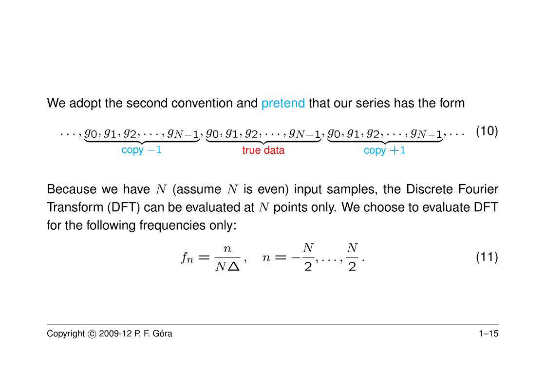
We adopt the second convention and pretend that our series has the form

. . . , g0, g1, g2, . . . , gN−1︸︷︷︸copy −1

, g0, g1, g2, . . . , gN−1︸︷︷︸true data

, g0, g1, g2, . . . , gN−1︸︷︷︸copy +1

, . . . (10)

Because we have N (assume N is even) input samples, the Discrete FourierTransform (DFT) can be evaluated at N points only. We choose to evaluate DFTfor the following frequencies only:

fn =n

N∆, n = −

N

2, . . . ,

N

2. (11)


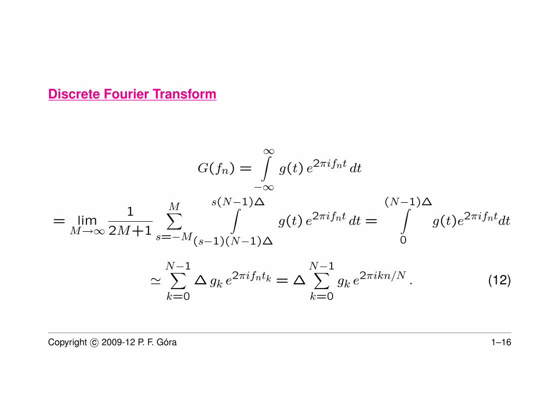
Discrete Fourier Transform

G(fn) =

∞∫−∞

g(t) e2πifnt dt

= limM→∞

1

2M+1

M∑s=−M

s(N−1)∆∫(s−1)(N−1)∆

g(t) e2πifnt dt =

(N−1)∆∫0

g(t)e2πifntdt

'N−1∑k=0

∆ gk e2πifntk = ∆

N−1∑k=0

gk e2πikn/N . (12)


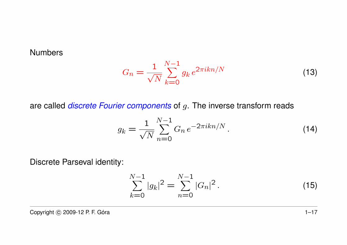
Numbers

Gn =1√N

N−1∑k=0

gk e2πikn/N (13)

are called discrete Fourier components of g. The inverse transform reads

gk =1√N

N−1∑n=0

Gn e−2πikn/N . (14)

Discrete Parseval identity:

N−1∑k=0

|gk|2 =N−1∑n=0

|Gn|2 . (15)


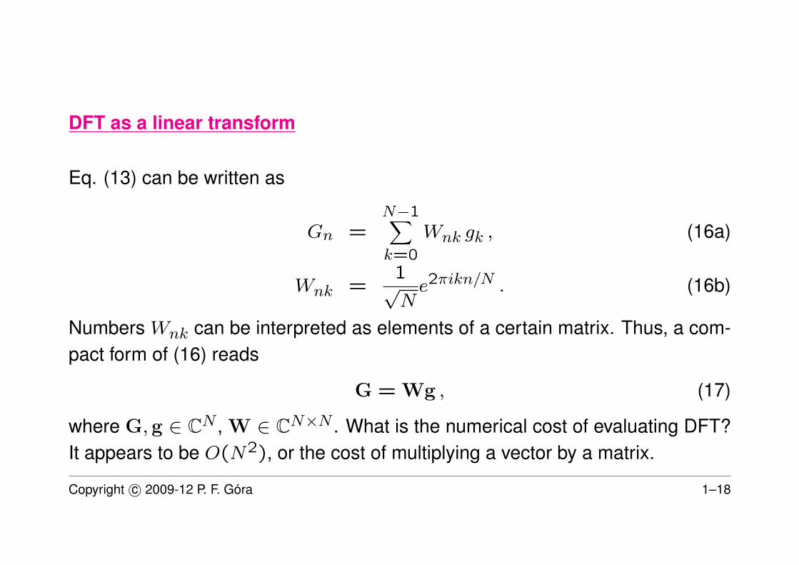
DFT as a linear transform

Eq. (13) can be written as

Gn =N−1∑k=0

Wnk gk , (16a)

Wnk =1√Ne2πikn/N . (16b)

Numbers Wnk can be interpreted as elements of a certain matrix. Thus, a com-pact form of (16) reads

G = Wg , (17)

where G, g ∈ CN , W ∈ CN×N . What is the numerical cost of evaluating DFT?It appears to be O(N2), or the cost of multiplying a vector by a matrix.


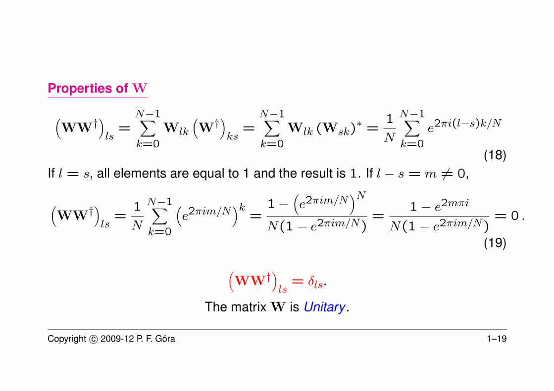
Properties of W

(WW†

)ls

=N−1∑k=0

Wlk

(W†

)ks

=N−1∑k=0

Wlk (Wsk)∗ =1

N

N−1∑k=0

e2πi(l−s)k/N

(18)If l = s, all elements are equal to 1 and the result is 1. If l − s = m 6= 0,

(WW†

)ls

=1

N

N−1∑k=0

(e2πim/N

)k=

1−(e2πim/N

)NN(1− e2πim/N)

=1− e2mπi

N(1− e2πim/N)= 0 .

(19)

(WW†

)ls

= δls.

The matrix W is Unitary .


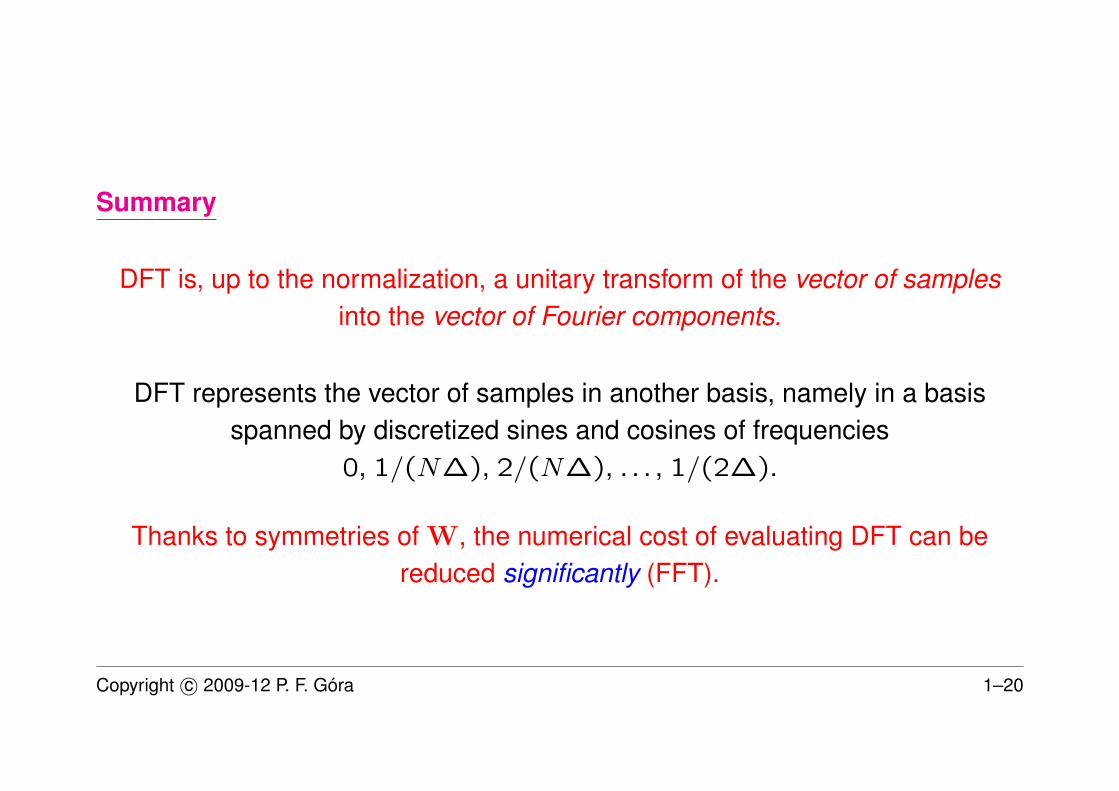
Summary

DFT is, up to the normalization, a unitary transform of the vector of samplesinto the vector of Fourier components.

DFT represents the vector of samples in another basis, namely in a basisspanned by discretized sines and cosines of frequencies

0, 1/(N∆), 2/(N∆), . . . , 1/(2∆).

Thanks to symmetries of W, the numerical cost of evaluating DFT can bereduced significantly (FFT).


Remarks

• Discrete Fourier components are periodic. In particular, G−N/2 = GN/2.

• Transforms spanned by sines or cosines only are also in use (one-sidedtransforms).

• The “signal” can be complex. If the signal is real, it is convenient to calculateits transform treating the signal as complex of half the length. Similarly,transforms of two real signals can be evaluated simultaneously. Symmetriesof DFT are then used to deconvolve the transforms.


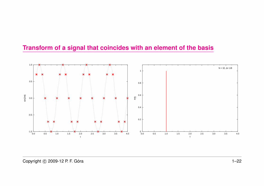
Transform of a signal that coincides with an element of the basis

-1.0

-0.5

0.0

0.5

1.0

0.0 0.5 1.0 1.5 2.0 2.5 3.0 3.5 4.0

sin(

2πt)

t

0

0.2

0.4

0.6

0.8

1

0.0 0.5 1.0 1.5 2.0 2.5 3.0 3.5 4.0P

(f)

f

N = 32, ∆= 1/8


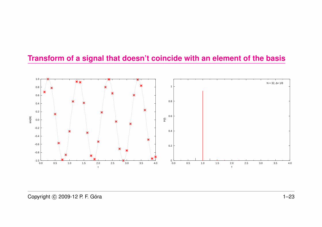
Transform of a signal that doesn’t coincide with an element of the basis

-1.0

-0.8

-0.6

-0.4

-0.2

0.0

0.2

0.4

0.6

0.8

1.0

0.0 0.5 1.0 1.5 2.0 2.5 3.0 3.5 4.0

sin(

6t)

t

0

0.2

0.4

0.6

0.8

1

0.0 0.5 1.0 1.5 2.0 2.5 3.0 3.5 4.0P

(f)

f

N = 32, ∆= 1/8


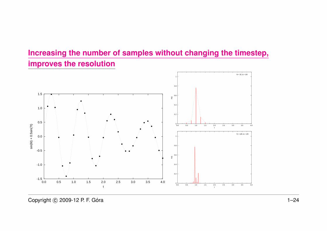
Increasing the number of samples without changing the timestep,improves the resolution

-1.5

-1.0

-0.5

0.0

0.5

1.0

1.5

0.0 0.5 1.0 1.5 2.0 2.5 3.0 3.5 4.0

sin(

6t)

+ 0

.5si

n(7t

)

t

0

0.2

0.4

0.6

0.8

1

0.0 0.5 1.0 1.5 2.0 2.5 3.0 3.5 4.0

P(f

)

f

N = 32, ∆ = 1/8

0

0.2

0.4

0.6

0.8

1

0.0 0.5 1.0 1.5 2.0 2.5 3.0 3.5 4.0

P(f

)

f

N = 128, ∆ = 1/8


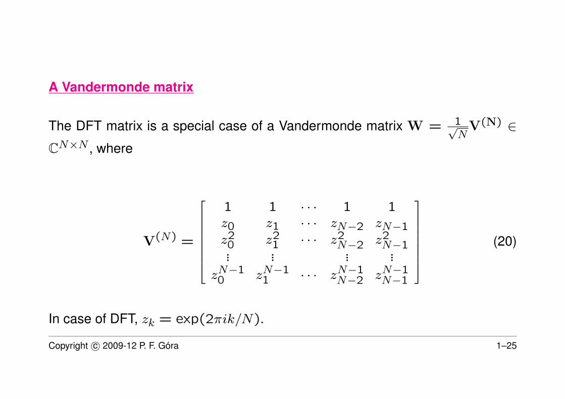
A Vandermonde matrix

The DFT matrix is a special case of a Vandermonde matrix W = 1√N

V(N) ∈CN×N , where

V(N) =

1 1 · · · 1 1z0 z1 · · · zN−2 zN−1z2

0 z21 · · · z2

N−2 z2N−1... ... ... ...

zN−10 zN−1

1 · · · zN−1N−2 zN−1

N−1

(20)

In case of DFT, zk = exp(2πik/N).


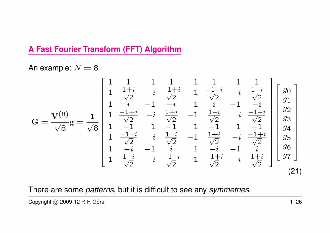
A Fast Fourier Transform (FFT) Algorithm

An example: N = 8

G =V(8)√

8g =

1√8

1 1 1 1 1 1 1 1

1 1+i√2

i −1+i√2−1 −1−i√

2−i 1−i√

21 i −1 −i 1 i −1 −i1 −1+i√

2−i 1+i√

2−1 1−i√

2i −1−i√

21 −1 1 −1 1 −1 1 −1

1 −1−i√2

i 1−i√2−1 1+i√

2−i −1+i√

21 −i −1 i 1 −i −1 i

1 1−i√2

−i −1−i√2−1 −1+i√

2i 1+i√

2

g0g1g2g3g4g5g6g7

(21)

There are some patterns, but it is difficult to see any symmetries.Copyright c© 2009-12 P. F. Góra 1–26

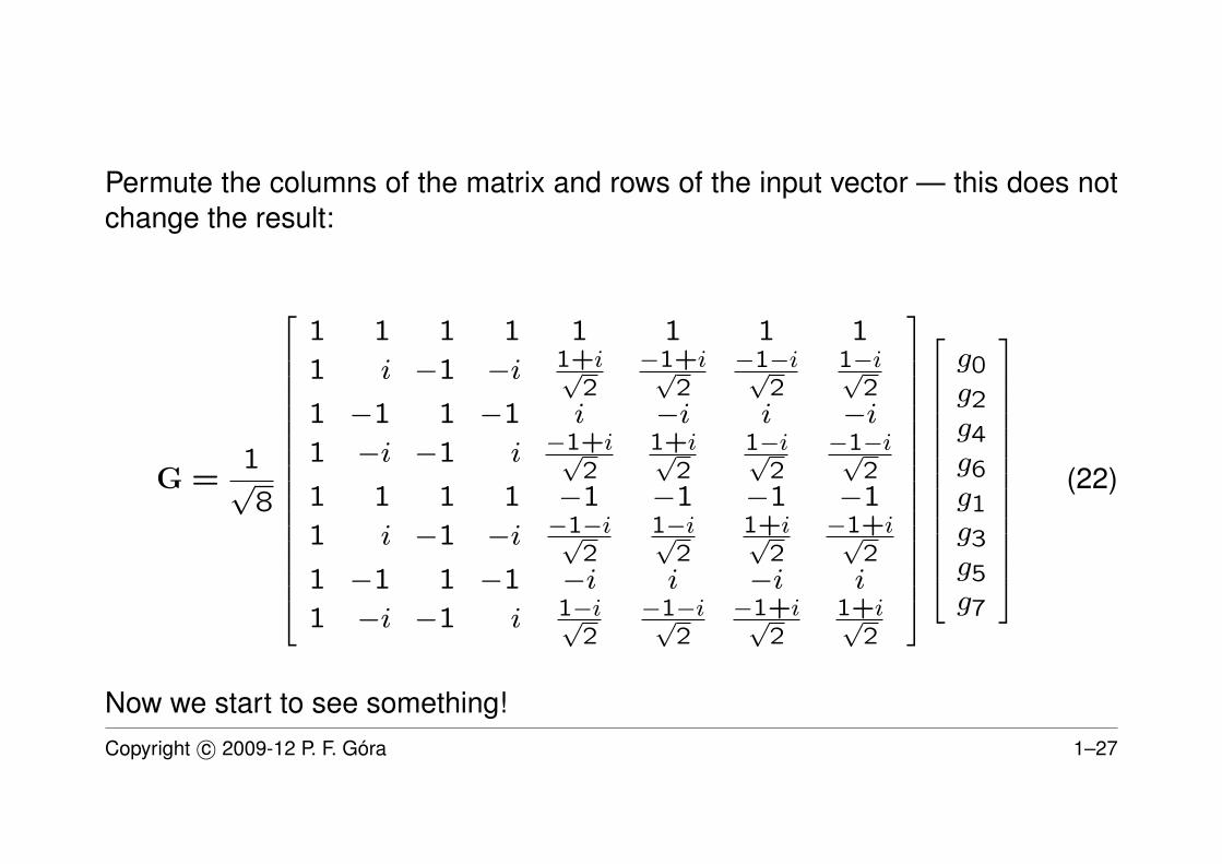
Permute the columns of the matrix and rows of the input vector — this does notchange the result:

G =1√8

1 1 1 1 1 1 1 1

1 i −1 −i 1+i√2

−1+i√2

−1−i√2

1−i√2

1 −1 1 −1 i −i i −i1 −i −1 i −1+i√

21+i√

21−i√

2−1−i√

21 1 1 1 −1 −1 −1 −1

1 i −1 −i −1−i√2

1−i√2

1+i√2

−1+i√2

1 −1 1 −1 −i i −i i

1 −i −1 i 1−i√2

−1−i√2

−1+i√2

1+i√2

g0g2g4g6g1g3g5g7

(22)

Now we start to see something!Copyright c© 2009-12 P. F. Góra 1–27

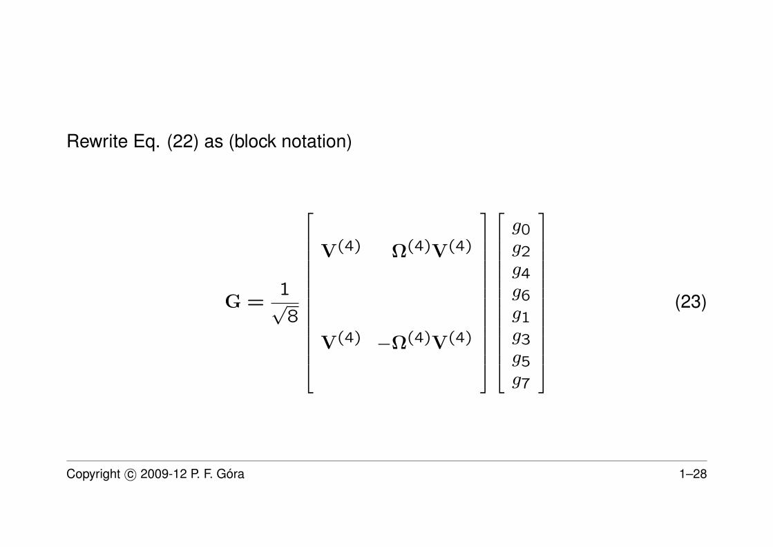
Rewrite Eq. (22) as (block notation)

G =1√8

V(4) Ω(4)V(4)

V(4) −Ω(4)V(4)

g0g2g4g6g1g3g5g7

(23)


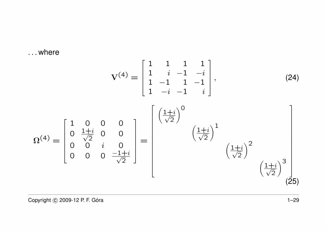
. . . where

V(4) =

1 1 1 11 i −1 −i1 −1 1 −11 −i −1 i

, (24)

Ω(4) =

1 0 0 0

0 1+i√2

0 0

0 0 i 0

0 0 0 −1+i√2

=

(1+i√

2

)0

(1+i√

2

)1

(1+i√

2

)2

(1+i√

2

)3

(25)


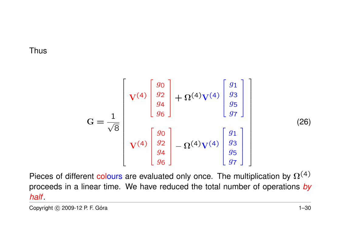
Thus

G =1√8

V(4)

g0g2g4g6

+ Ω(4)V(4)

g1g3g5g7

V(4)

g0g2g4g6

−Ω(4)V(4)

g1g3g5g7

(26)

Pieces of different colours are evaluated only once. The multiplication by Ω(4)

proceeds in a linear time. We have reduced the total number of operations byhalf .Copyright c© 2009-12 P. F. Góra 1–30

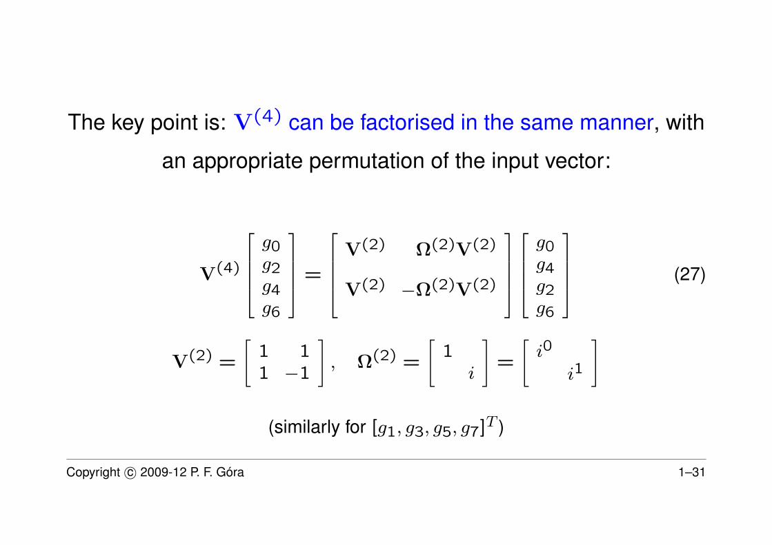
The key point is: V(4) can be factorised in the same manner, with

an appropriate permutation of the input vector:

V(4)

g0g2g4g6

=

V(2) Ω(2)V(2)

V(2) −Ω(2)V(2)

g0g4g2g6

(27)

V(2) =

[1 11 −1

], Ω(2) =

[1

i

]=

[i0

i1

]

(similarly for [g1, g3, g5, g7]T )


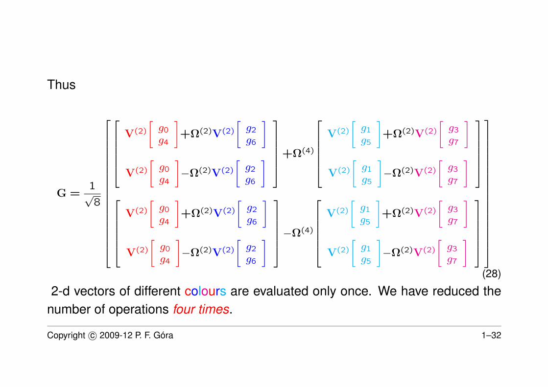
Thus

G =1√8

V(2)

[g0

g4

]+Ω(2)V(2)

[g2

g6

]

V(2)

[g0

g4

]−Ω(2)V(2)

[g2

g6

]+Ω(4)

V(2)

[g1

g5

]+Ω(2)V(2)

[g3

g7

]

V(2)

[g1

g5

]−Ω(2)V(2)

[g3

g7

]

V(2)

[g0

g4

]+Ω(2)V(2)

[g2

g6

]

V(2)

[g0

g4

]−Ω(2)V(2)

[g2

g6

]−Ω(4)

V(2)

[g1

g5

]+Ω(2)V(2)

[g3

g7

]

V(2)

[g1

g5

]−Ω(2)V(2)

[g3

g7

]

(28)

2-d vectors of different colours are evaluated only once. We have reduced thenumber of operations four times.


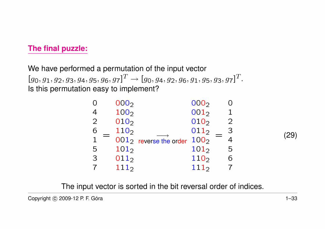
The final puzzle:

We have performed a permutation of the input vector[g0, g1, g2, g3, g4, g5, g6, g7]T → [g0, g4, g2, g6, g1, g5, g3, g7]T .Is this permutation easy to implement?

04261537

=

00021002010211020012101201121112

−→reverse the order

00020012010201121002101211021112

=

01234567

(29)

The input vector is sorted in the bit reversal order of indices.Copyright c© 2009-12 P. F. Góra 1–33

This algorithm easily generalizes to any N = 2s, s ∈ N.

The need to evaluate terms like sin(nπN

), cos

(nπN

)is also reduced — there is

no need to call library functions sin(·), cos(·). On each stage of factorisationsa root of i is evaluated only once with ready-to-use formulas. Then only the

powers of that root are evaluated.

What is the final numerical cost?


Each factorisation reduces the number of operations by half.

There are log2N factorisations.

The numerical cost of the FFT algorithm equals

O(N log2N)

For example, for N = 65536 = 216 FFT reduces the numerical cost ofevaluating DFT more than four thousand times.


Remarks

• Similar algorithms can be constructed for N = 3s, N = 5s and, in general,any N = qs, where q prime. The numerical cost is O(N logqN).

• Good libraries automatically factorise also matrices of the size N =

qs11 q

s22 · · · q

smm , where q1, q2, . . . , qm are small primes.

• If we analyse a series that we calculate, we can control its length and weshould make it a power of a small prime. If we analyse an “experimental”series, it is wise either to truncate it or to pad it with zeros to a power of asmall prime.

• There are “fast” versions of the one-sided (sine or cosine) transforms.

• There are many FFT packages over the Internet; some of them are free andgood. I recommend The Fastest Fourier Transform in the West,http://www.fftw.com.


http://www.fftw.com

time series analysis: 1. sampling and dft

Documents