time series analysis of production and price of cattle and...
TRANSCRIPT

1921
ISSN 2286-4822
www.euacademic.org
EUROPEAN ACADEMIC RESEARCH
Vol. V, Issue 4/ July 2017
Impact Factor: 3.4546 (UIF)
DRJI Value: 5.9 (B+)
Time Series Analysis of Production and Price of
Cattle and Milkfish in the Philippines
ARIANE S. ANGELES
Philippine Statistics Authority
PHYLORD D. DAYAG
Global Quest Consultancy Group Incorporated
ROLAND A. LAZAN
Newborn Screening Center – Southern Luzon
Abstract:
The purpose of the study is to forecast quarterly production
and farmgate prices of Cattle and Milkfish in the Philippines from
2017-2021. This paper takes into account the quarterly data of Cattle
from 1980-2016 and Milkfish from 2002-2016; and quarterly farmgate
prices of cattle and milkfish from 1990-2016 gathered from Philippine
Statistics Authority which serve as the central statistical authority of
the Philippine government on primary data collection. Autoregressive
Integraded Moving Average (ARIMA) was used to forecast the
quarterly production of Cattle and Milkfish in the Philippines while
Autoregressive Moving Average was used for Farmgate prices. Models
with lowest Akaike Information Critera (AIC) and Bayesian
information criterion (BIC) was considered as best fitted model. Best
fitted model obtained for Cattle production is ARIMA(4,1,2) and
ARIMA(12,1,12) for Milkfish Production. ARMA(12,12) and
ARMA(5,10) is the best fitted model respectively for cattle and milkfish
farmgate prices.
Key words: ARIMA, Cattle Production, Milkfish Production Cattle
Farmgate Price, Milkfish Farmgate Price, AIC, BIC

Ariane S. Angeles, Phylord D. Dayag, Roland A. Lazan- Time Series Analysis of
Production and Price of Cattle and Milkfish in the Philippines
EUROPEAN ACADEMIC RESEARCH - Vol. V, Issue 4 / July 2017
1922
I. Introduction
Raising Cattle in the Philippines is mostly backyard type and
traditionally led by the private sector Commercial feedlot
fattening operation. It has been evaluated, however, that beef
cattle raising in the country has a comparative advantage over
other animal production ventures considering the increasing
demand for beef; ability to transform low-quality and fibrous
feed materials; availability of other forages and favorable
climate for fodder production and adequate processing
technologies and increased productivity (source:
pcarrd.dost.gov.ph) Livestock raising is being recognized as a
source of income for rural communities. In the citation of A.C.
Castillo, the raising of farm animals is still on a small scale
basis since it is intimately tied-in with farmers' activities and
way of life. Cattle is raised for drought purposes and as source
of cash in time of needs. Also, these animals offer a means
whereby crop products and farm residues as well as native
vegetation in uncultivated areas are converted into meat, milk,
hides and other by-products. Aside from livestock products, the
sustainability of fisheries and aquaculture is also relevant in an
archipelago like the Philippines, where millions of families rely
for their daily sustenance and income. According to Food and
Agriculture Organization of the United Nations, aquaculture is
making significant headway as the fastest-growing food sector.
Among the sub-sectors in fisheries, it provides the most
potential to reduce hunger and improve nutrition, alleviate
poverty, generate economic growth, and ensure better use of
natural resources.
Milkfish is one of the most important farmed fish species
in the Philippines. Only a small volume out of the total
production came from the wild (source: pcarrd.dost.gov.ph).
Milkfish is an important commodity that is widely cultured in
the Philippines. It is good to invest in Milkfish because of its
high demand for food consumption in the Philippines.

Ariane S. Angeles, Phylord D. Dayag, Roland A. Lazan- Time Series Analysis of
Production and Price of Cattle and Milkfish in the Philippines
EUROPEAN ACADEMIC RESEARCH - Vol. V, Issue 4 / July 2017
1923
Forecasting production and price of cattle and fish are
important for potential users and policy makers by examining
results and recommendations based on their trend and future
values. This study will forecast the production and farmgate
price of Cattle and Milkfish. In doing so, we have to review first
the trend of the selected commodities in agriculture; investigate
the model for forecasting selected commodities, forecast the
future values of production and price; make recommendations
based on the output.
The top 10 countries by forecast growth in beef, pork and
chicken consumption from 2011 to 2021 include the Philippines.
This was declared by United Kingdom-based think tank
Chatham House based on projected consumption increases from
Food and Agricultural Policy Research Institute-Iowa State
University, 2012 (Plotnek, 2017). Relating this research to
consumption is important because forecasting production can
be based on consumption. Forecasting production or the
capacity to produce can lead policy makers to look for
agricultural commodity importation restriction and look for
alternative products to produce to sustain consumption.
Increasing Agricultural commodity production means increase
employment rate and this will help the economy.
1.1 Objective of the Study
The main objective of study is to forecast the production and
farmgate price of Cattle and Milkfish in the Philippines. More
specifically, the study aims:
1. To present the trend in production and price of cattle
and milkfish in the country;
2. To present the best fitted model in forecasting the
production and price;
3. To compare the actual data and forecasted data; and
4. To forecast production and farmgate price of cattle
and milkfish from 2017-2021.

Ariane S. Angeles, Phylord D. Dayag, Roland A. Lazan- Time Series Analysis of
Production and Price of Cattle and Milkfish in the Philippines
EUROPEAN ACADEMIC RESEARCH - Vol. V, Issue 4 / July 2017
1924
1.2 Statement of the Problem
The study was conducted to formulate a model in forecasting
production and farmgate prices of cattle and milkfish in the
Philippines using Autoregressive Moving Average (ARMA) and
Autoregressive Integrated Moving Average (ARIMA).
Specifically, the study wants to answer the following questions:
1. What is the trend in production and price of cattle
and milkfish in the country;
2. What model to use to forecast production and
Farmgate price;
3. What is the difference between the actual data and
forecasted data; and
4. What is the forecast and trend of the production and
prices of cattle and milkfish from 2017 to 2021?
1.3 Significance of the Study
This research focuses on predicting future production and
prices of Cattle and Milkfish in the Philippines through
forecasting technique. By examining the result and
recommendation of the study, policy makers and potential users
can imposed necessary steps to improve the production and
farmgate prices of cattle and milkfish. And also, this study can
be helpful for new business growth related to cattle and
milkfish.
1.4 Scope and Limitation
Data was collected from the Philippine Statistics Authority
which serve as the central statistical authority of the Philippine
government on primary data collection. This study used
quarterly production data of Cattle from 1980-2016 and
Milkfish from 2002-2016; and quarterly farmgate prices of
cattle and milkfish from 1990-2016.

Ariane S. Angeles, Phylord D. Dayag, Roland A. Lazan- Time Series Analysis of
Production and Price of Cattle and Milkfish in the Philippines
EUROPEAN ACADEMIC RESEARCH - Vol. V, Issue 4 / July 2017
1925
1.5 Research Paradigm
Figure 1. Research Paradigm
II. Review of Related Literature
2.1 Foreign Studies
T. Jai Sakar, et al (2010). Propose a technique using ARIMA
model for cattle production in Tamilnadu. The estimated
results indicate that there an increase in the cattle production
which will improve the economy of the state. This provides
evidence in favor of Box-Jenkins methodology as it applies to
cattle production and future efficiency.
Jin, Power, & Elbakidze, 2008. Forecasting prices with
structural econometric models requires forecasts of the relevant
exogenous and lagged endogenous variables which are
considered to be exogenous in estimation. While these forecasts
can be obtained in a recursive manner, forecasts of exogenous
variables often present problems for econometric model users
Therefore, there was progressive on forecasting cattle prices
from structural models to the univariate ARIMA models by Box
and Jenkins that are based on current and past observations of
the particular data series with no exogenous variables included.
Lazaro M. And Lazaro W. (2013) Fisheries forecasting
is a very important tool for fisheries managers and scientists to
enable them to decide on sustainable management issues Time
series models have been used to forecast catches in fisheries
sectors in different countries but to the contrary, Malaŵi has
lagged behind in using time series model in forecasting. The

Ariane S. Angeles, Phylord D. Dayag, Roland A. Lazan- Time Series Analysis of
Production and Price of Cattle and Milkfish in the Philippines
EUROPEAN ACADEMIC RESEARCH - Vol. V, Issue 4 / July 2017
1926
study considered Autoregressive (AR), Moving Average (MA)
and Autoregressive Integrated Moving Average (ARIMA)
processes to select the appropriate stochastic model for
forecasting annual commercial chambo catch from Lake
Malawi. Based on ARIMA (p, d, q) and its components ACF,
PACF, Normalized BIC, Box-Ljung Q statistics and residuals
estimated, ARIMA (1, 1, 0) was selected. Based on the selected
model, it could be forecasted that the commercial chambo catch
would increase to 854 tonnes in 2020 from 437 tonnes in 2010
2.2 Local Studies
We want to know the future production of the said
agricultural commodities based on past productions, this
information to decision makers, it is important in many ways to
the economy. ARMA (Autoregressive Moving Average) and
Autoregressive Interated Moving Average model was use to
forecast production and farmgate prices. It has been found that
in terms of forecast ability ARMA models outperform AR
models, when following for the same degrees of freedom. Also,
the models with separate specification of a seasonal component
do better than models where seasonal terms are modeled jointly
with other components of the time series. Eventually, the
models with a trend displaying the structural break in 1999
outperform other models. Interestingly enough, in the context
of the sample examined, the standard in-sample model
selection criteria provide rather poor guidance in identifying
the best model for out-of-sample forecasting (Stovicek, 2007). A
study found that ARMA models performed best for Crop yield
prediction (Choudhury & Jones, 2014). Another study use
ARMA for the prediction of Rainfall (Bugroho & Simanjuntak
2014).

Ariane S. Angeles, Phylord D. Dayag, Roland A. Lazan- Time Series Analysis of
Production and Price of Cattle and Milkfish in the Philippines
EUROPEAN ACADEMIC RESEARCH - Vol. V, Issue 4 / July 2017
1927
III. Methodology
3.1 Statistical Tool
Statistical Software: Econometric Eviews used by researchers
to investigate the data series, formulate ARMA or ARIMA
model and forecast future values based on the selected model.
3.2 Statistical Treatment
3.2.1 Data Preparation
Plot the series data to capture the possible trend and
seasonality. Use Correlogram and examine ACF for
stationarity. If the series is not stationary, take first
differencing. Use Augmented Dickey-Fuller (ADF) Test for
formal test. Once model is stationary proceed to model
identification and estimation
3.2.1.1 Test for Stationarity: Augmented Dickey-Fuller
(ADF) Test
The stationarity or otherwise of a series can strongly influence
its behavior and properties. A series is said to be (weakly or
covariance) stationary if the mean and autocovariances of the
series do not depend on time. Any series that is not stationary
is said to be nonstationary or has unit root. So having a unit
root means:
ρ1 =1 in yt = ρ1 yt-1 + ρ2 Δyt-1 + ρ3Δyt-2 + ε t or equivalently
1-ρ1 =0 in Δyt = (ρ1-1) yt-1 +
ρj (Δyt-j+1) + ε t
3.2.2. Model Identification and Estimation
Examine the ACF (for Moving average term) and PACF (for
Autoregressive term) of the stationary series for possible
ARIMA (Autoregressive Integrated Moving Average) model to
estimate. Estimate the Models, if the parameters are
significant proceed to Diagnostic Checking.

Ariane S. Angeles, Phylord D. Dayag, Roland A. Lazan- Time Series Analysis of
Production and Price of Cattle and Milkfish in the Philippines
EUROPEAN ACADEMIC RESEARCH - Vol. V, Issue 4 / July 2017
1928
3.2.3 Residual diagnostic Checking
The model should past residual diagnostic checking to be
considered as candidate model for forecasting.
3.2.3.1 Ljung–Box test
A type of statistical test of whether any of a group of
autocorrelations of a time series are different from zero. Instead
of testing randomness at each distinct lag, it tests the "overall"
randomness based on a number of lags, and is therefore a
portmanteau test.
The Ljung–Box test may be defined as: Ho: The data are
independently distributed, Ha: The data are not independently
distributed; they exhibit serial correlation.
The test statistic is:
where n is the sample size, is the sample autocorrelation
at lag k, and h is the number of lags being tested . Under Ho the
statistic Q follows a . For significance level α, the critical
region for rejection of the hypothesis of randomness is.
where is the α-quantile of the chi-
squared distribution with h degrees of freedom.
The Ljung–Box test is rarely used in autoregressive
integrated moving average (ARIMA) modeling. It is applied to
the residuals of a fitted ARIMA model, not the original series,
and in such applications the hypothesis actually being tested is
that the residuals from the ARIMA model have no
autocorrelation. When testing the residuals of an estimated
ARIMA model, the degrees of freedom need to be adjusted to
reflect the parameter estimation.
3.2.3.2 Correlogram
Correlogram is an aid to interpret a set of ACF and PACF
where, sample autocorrelations are plotted against lag h. In
Ariane S. Angeles, Phylord D. Dayag, Roland A. Lazan- Time Series Analysis of
Production and Price of Cattle and Milkfish in the Philippines
EUROPEAN ACADEMIC RESEARCH - Vol. V, Issue 4 / July 2017
1929
addition, correlograms are used in the model identification
stage for Box–Jenkins autoregressive moving average time
series models. Autocorrelations should be near-zero for
randomness; if the analyst does not check for randomness, then
the validity of many of the statistical conclusions becomes
suspect. The Correlogram is an excellent way of checking for
such randomness.
3.2.3.3 Normality test
In statistics, the Jarque–Bera test is a goodness-of-fit test of
whether sample data have the skewness and kurtosis matching
a normal distribution. The test is named after Carlos Jarque
and Anil K. Bera. A large p-value and hence failure to reject
this null hypothesis is a good result. It means that it is
reasonable to assume that the errors have a normal
distribution. The residuals should be normally distributed so
that the t–statistics used to evaluate the significance of AR and
MA terms are valid. Jarque-Bera test have the formula:
, ,
where x is each observation, n is the sample size, s is the
standard deviation, k3 is skewness, and k4 is kurtosis.
3.2.3.4 Heteroskedasticity: White Test
Residuals from an ARIMA model should show a constant
variance in order to support proper calculation of the unbiased
standard errors that are part of the t- statistics and F-statistics
required for hypothesis testing. White’s test attempts to create
whether or not the variance is changing.
Breusch–Pagan test is used to test for heteroskedasticity in
a linear regression model.
Ariane S. Angeles, Phylord D. Dayag, Roland A. Lazan- Time Series Analysis of
Production and Price of Cattle and Milkfish in the Philippines
EUROPEAN ACADEMIC RESEARCH - Vol. V, Issue 4 / July 2017
1930
Procedure:
Under the classical assumptions, ordinary least squares is
the best linear unbiased estimator (BLUE), i.e., it is unbiased
and efficient. It remains unbiased under heteroskedasticity, but
efficiency is lost. Before deciding upon an estimation method,
one may conduct the Breusch–Pagan test to examine the
presence of heteroskedasticity. The Breusch–Pagan test is
based on models of the type for the variances of
the observations where explain the
difference in the variances. The null hypothesis is equivalent to
the (p-1) parameter restrictions: The
following Lagrange multiplier (LM) yields the test statistic for
the Breusch–Pagan test:
This test is analogous to following the simple three-step
procedure:
Step 1: Apply OLS in the model and compute the
regression residuals.
Step 2: Perform the auxiliary regression
Always, z could be partly
replaced by independent variables x
Step 3: The test statistic is the result of the coefficient of
determination of the auxiliary regression in Step 2 and sample
size n with:
The test statistic is asymptotically distributed as under
the null hypothesis of homoscedasticity.
3.2.3.5 Serial Correlation
Testing for autocorrelation in a time series is a common task for
researchers working with time-series data.

Ariane S. Angeles, Phylord D. Dayag, Roland A. Lazan- Time Series Analysis of
Production and Price of Cattle and Milkfish in the Philippines
EUROPEAN ACADEMIC RESEARCH - Vol. V, Issue 4 / July 2017
1931
Breusch-Godfrey Serial Correlation LM test
Test used for AR (1) and higher orders of serial correlation. The
Breusch-Godfrey Test regress the residuals on the original
regressors and lagged residuals up to the specified lag order.
(EViews User’s Guide, p 338)
The Breusch–Godfrey serial correlation LM test is a test
for autocorrelation in the errors in a regression model. It makes
use of the residuals from the model being considered in
a regression analysis, and a test statistic is derived from these.
The null hypothesis is that there is no serial correlation of any
order up to p.
Procedure:
Consider a linear regression of any form, for example
where the errors might follow an AR(p) autoregressive scheme,
as follows:
The simple regression model is first fitted by ordinary least
squares to obtain a set of sample residuals . Breusch and
Godfrey proved that, if the following auxiliary regression model
is fitted
and if the usual R2 statistic is calculated for this model, then
the following asymptotic approximation can be used for the
distribution of the test statistic ,when the null
hypothesis , holds (that is, there is no serial
correlation of any order up to p). Here n is the number of data-
points available for the second regression, that for ,

Ariane S. Angeles, Phylord D. Dayag, Roland A. Lazan- Time Series Analysis of
Production and Price of Cattle and Milkfish in the Philippines
EUROPEAN ACADEMIC RESEARCH - Vol. V, Issue 4 / July 2017
1932
where T is the number of observations in the basic series. Note
that the value of n depends on the number of lags of the error
term (p)
3.2.4 Forecasting and Forecast Evaluation Measures
Use the model to construct forecast, Graph the forecast against
the actual values. Use AIC and BIC to choose the parsimonious
model for forecasting.
3.2.4.1 Akaike Information Critera (AIC)
The Akaike Information Critera (AIC) is a generally used
measure of a statistical model. It basically measures the
goodness of fit, and the simplicity/parsimony, of the model into
a single statistic. It can be written as
( ) ( )
where is the likelihood of the data, k=1 if c≠0 and k=0 if c=0.
Note that the last term in parentheses is the number of
parameters in the model (including the variance of the
residuals).
3.2.4.2 Bayesian information criterion (BIC) or Schwarz
criterion (also SBC, SBIC)
Bayesian information criterion (BIC) or Schwarz
criterion (also SBC, SBIC) is a criterion for model selection
among a finite set of models; the model with the lowest BIC is
preferred. It is based, in part, on the likelihood function and it
is closely related to the Akaike information criterion (AIC).
When fitting models, it is possible to increase the
likelihood by adding parameters, but doing so may result in
overfitting. Both BIC and AIC attempt to resolve this problem
by introducing a penalty term for the number of parameters in
the model; the penalty term is larger in BIC than in AIC.
The BIC is formally defined as
( ) ( )̂

Ariane S. Angeles, Phylord D. Dayag, Roland A. Lazan- Time Series Analysis of
Production and Price of Cattle and Milkfish in the Philippines
EUROPEAN ACADEMIC RESEARCH - Vol. V, Issue 4 / July 2017
1933
20
30
40
50
60
70
80
1980 1985 1990 1995 2000 2005 2010 2015
CATTLE
Where ̂ is the maximized value of the likelihood function of the
model, n = the number of data points, and k = the number of
free parameters to be estimated.
IV. Results and Discussion
4.1 TIME SERIES PLOT
4.1.1 CATTLE PRODUCTION
Figure 2. Time Series plot of Cattle Production in the Philippines
1980Q1 – 2016Q4
A perusal of Figure 2 reveals an increasing trend in the cattle
production in the Philippines over the years. At the same time,
the figure also shows that the production is highest during the
first and third quarter and lowest during second and fourth
quarter during the year.
Dickey fuller test was used to test if unit root exist for
Cattle production. Actual series is not stationary but after first
differencing the series become stationary (See Appendix A,
Table 1) After the first differencing the time series data on the
production became stationary. (See Appendix A, Table 2)

Ariane S. Angeles, Phylord D. Dayag, Roland A. Lazan- Time Series Analysis of
Production and Price of Cattle and Milkfish in the Philippines
EUROPEAN ACADEMIC RESEARCH - Vol. V, Issue 4 / July 2017
1934
40,000
50,000
60,000
70,000
80,000
90,000
100,000
110,000
120,000
130,000
02 03 04 05 06 07 08 09 10 11 12 13 14 15 16
MILKFISH
30
40
50
60
70
80
90
100
94 96 98 00 02 04 06 08 10 12 14 16
CATTLE_PRICE
4.1.2 MILKFISH PRODUCTION
Figure 3. Time Series Plot Fish Production in the Philippines 1980Q1
– 2016Q4
Analysis of Figure 3 reveals an increasing movement in the
Milkfish production in the Philippines over the years. At the
same time, the figure also shows that the production is highest
during the second and fourth quarter and lowest during first
and third quarter during the year.
Dickey fuller test was used to test if unit root exist for
Milkfish production. Actual series is not stationary but after
first differencing the series become stationary (See Appendix A,
Table 1) After the first differencing the time series data on the
production became stationary. (See Appendix A, Table 2)
4.1.3 Cattle Farmgate Price
Figure 4. Time Series Plot of Cattle Farmgate Price in the Philippines
from1980Q1 – 2016Q4
Ariane S. Angeles, Phylord D. Dayag, Roland A. Lazan- Time Series Analysis of
Production and Price of Cattle and Milkfish in the Philippines
EUROPEAN ACADEMIC RESEARCH - Vol. V, Issue 4 / July 2017
1935
40
50
60
70
80
90
100
110
120
130
90 92 94 96 98 00 02 04 06 08 10 12 14 16
MF_PRICE
Analysis of Figure 4 reveals an increasing movement in
farmgate price of cattle in the Philippines over the years.
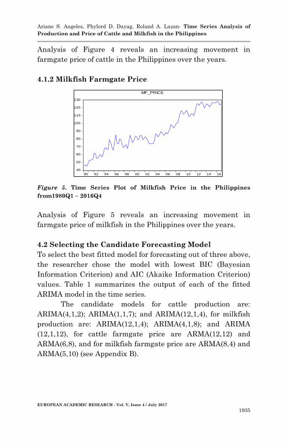
4.1.2 Milkfish Farmgate Price
Figure 5. Time Series Plot of Milkfish Price in the Philippines
from1980Q1 – 2016Q4
Analysis of Figure 5 reveals an increasing movement in
farmgate price of milkfish in the Philippines over the years.
4.2 Selecting the Candidate Forecasting Model
To select the best fitted model for forecasting out of three above,
the researcher chose the model with lowest BIC (Bayesian
Information Criterion) and AIC (Akaike Information Criterion)
values. Table 1 summarizes the output of each of the fitted
ARIMA model in the time series.
The candidate models for cattle production are:
ARIMA(4,1,2); ARIMA(1,1,7); and ARIMA(12,1,4), for milkfish
production are: ARIMA(12,1,4); ARIMA(4,1,8); and ARIMA
(12,1,12), for cattle farmgate price are ARMA(12,12) and
ARMA(6,8), and for milkfish farmgate price are ARMA(8,4) and
ARMA(5,10) (see Appendix B).

Ariane S. Angeles, Phylord D. Dayag, Roland A. Lazan- Time Series Analysis of
Production and Price of Cattle and Milkfish in the Philippines
EUROPEAN ACADEMIC RESEARCH - Vol. V, Issue 4 / July 2017
1936
Table 1
AIC AND BIC Values of fitted ARIMA Models
Series Data ARIMA Model AIC BIC R-squared MAPE
Cattle Production (4,1,2) 3.94 4.02 94.76 2.36
(1,1,7) 3.95 4.01 94.63 2.54
(12,1,4) 4.52 4.6 91.09 3.49
Milkfish Production (12,1,4) 20.08 20.2 95.04 3.59
(4,1,8) 19.58 19.73 96.75 2.63
12,1,12 19.59 19.71 96.96 2.66
Cattle Farmgate Price (12,12) 4.11 4.2 98.96 1.8
(6,8) 4.12 4.26 99.04 1.91
Milkfish Farmgate Price (8,4) 5.21 5.1 98.15 1.88
(5,10) 5.19 5.08 98.23 2.75
The table shows that the lowest AIC and BIC values for cattle
production is the ARIMA(4,1,2) model with (p=4, d=1 and q=2),
for milkfish production is the ARIMA(12,1,12) model with
(p=12, d=1 and q=12), for cattle farmgate price is the ARMA
(12, 12) model with (p=12 d=1 q=12), for milkfish farmgate
price is the ARMA (5,10) model with (p=5, d=0 and q=10), hence
this model can be the best predictive model for making
forecasts for future production and price of cattle and milkfish
values.
4.3 Actual versus Forecast
Figure 6. Actual Cattle Production versus Forecasted Cattle
Production
Figure 6 above shows the forecasted cattle production follow the
trend of the actual value. The forecast values follows the trend
of the actual data on cattle production.

Ariane S. Angeles, Phylord D. Dayag, Roland A. Lazan- Time Series Analysis of
Production and Price of Cattle and Milkfish in the Philippines
EUROPEAN ACADEMIC RESEARCH - Vol. V, Issue 4 / July 2017
1937
Figure 7. Actual Milkfish Production versus Forecast Milkfish
Production
Figure 7 above shows the forecasted milkfish production follow
the trend of the actual value.
Figure 8. Actual Cattle Farmgate Price versus Forecast Cattle
Farmgate Price
The figure 8 above shows the forecasted farmgate price of cattle
follow the trend of the actual value.
Figure 9. Actual Milkfish Farmgate Price versus Forecast Milkfish
Farmgate Price

Ariane S. Angeles, Phylord D. Dayag, Roland A. Lazan- Time Series Analysis of
Production and Price of Cattle and Milkfish in the Philippines
EUROPEAN ACADEMIC RESEARCH - Vol. V, Issue 4 / July 2017
1938
The figure 9 above shows the forecasted farmgate price of
milkfish follow the trend of the actual value.
4.1.3 Forecast from the Best Model
The production model for cattle is a function of the past values
of cattle production with autoregressive of order four and
moving average of order two.
The forecasting model for cattle production is
statistically significant as shown by the computed p-value of
the F-statistics, 0.00. The coefficient of determination suggests
that the independent variable explain 94 percent of the total
variation in cattle production. On the average, the model’s
forecast is off by 2.36 percent of the actual production.
(Appendix B, Table 1)
Table 2
ARIMA (4,1,2) Forecasted Cattle Production from 2017Q1-2021Q4
Quarter Production in '000 metric ton Percent change
2016 2017F 2018F 2019F 2020F 2021F 17F/16 18F/17F 19F/18F 20F/19F 21F/20F
Q1 61.09 62.37 63.63 64.67 65.50 66.16 2.10 2.02 1.62 1.29 1.00
Q2 70.28 72.14 73.81 75.31 76.68 77.92 2.64 2.31 2.04 1.81 1.62
Q3 59.86 60.65 61.30 61.82 62.25 62.59 1.32 1.07 0.86 0.69 0.55
Q4 79.18 80.25 81.14 81.88 82.50 83.02 1.35 1.11 0.91 0.76 0.63
The estimated cattle production for 2016 Q4 is 79.18 thousand
metric tons which is 1.83 percent higher as compared to the
same period last year. Based on the prediction result that there
is a positive increase in cattle production in all quarters up to
2021.
Figure 10. Graph of ARIMA (4,1,2) Forecasted Cattle Production from
2017Q1-2021Q4
20
30
40
50
60
70
80
90
1985 1990 1995 2000 2005 2010 2015 2020
CATTLEF ± 2 S.E.
Forecast: CATTLEF
Actual: CATTLE
Forecast sample: 1980Q1 2021Q4
Adjusted sample: 1981Q2 2021Q4
Included observations: 162
Root Mean Squared Error 1.581546
Mean Absolute Error 1.155261
Mean Abs. Percent Error 2.356067
Theil Inequality Coefficient 0.013791
Bias Proportion 0.001994
Variance Proportion 0.002288
Covariance Proportion 0.995717
Ariane S. Angeles, Phylord D. Dayag, Roland A. Lazan- Time Series Analysis of
Production and Price of Cattle and Milkfish in the Philippines
EUROPEAN ACADEMIC RESEARCH - Vol. V, Issue 4 / July 2017
1939
The production model for milkfish is a function of the past
values of milkfish production with autoregressive of order
twelve and moving average of order twelve. Below is the
estimated equation:
The forecasting model for milkfish production is
statistically significant as shown by the computed p-value of
the F-statistics, 0.00. The coefficient of determination suggests
that the independent variable explain 99 percent of the total
variation in milkfish production. On the average, the model’s
forecast is off by 2.66 percent of the actual production.
(Appendix C).
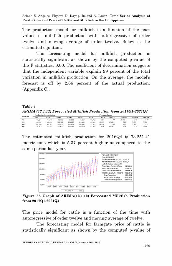
Table 3
ARIMA (12,1,12) Forecasted Milkfish Production from 2017Q1-2021Q4
Quarter Production in metric ton Percent change
2016 2017F 2018F 2019F 2020F 2021F 17F/16 18F/17F 19F/18F 20F/19F 21F/20F
Q1 73,251 74,790 75,850 75,307 76,347 77,942 2.10 1.42 (0.72) 1.38 2.09
Q2 100,827 100,526 100,402 103,057 102,424 102,342 (0.30) (0.12) 2.64 (0.61) (0.08)
Q3 108,599 105,102 107,575 112,429 108,952 111,643 (3.22) 2.35 4.51 (3.09) 2.47
Q4 119,978 123,981 117,610 125,580 130,250 123,046 3.34 (5.14) 6.78 3.72 (5.53)
The estimated milkfish production for 2016Q4 is 73,251.41
metric tons which is 5.37 percent higher as compared to the
same period last year.
Figure 11. Graph of ARIMA(12,1,12) Forecasted Milkfish Production
from 2017Q1-2021Q4
The price model for cattle is a function of the time with
autoregressive of order twelve and moving average of twelve.
The forecasting model for farmgate price of cattle is
statistically significant as shown by the computed p-value of
40,000
60,000
80,000
100,000
120,000
140,000
160,000
2004 2006 2008 2010 2012 2014 2016 2018 2020
MILKFISHF ± 2 S.E.
Forecast: MILKFISHF
Actual: MILKFISH
Forecast sample: 2002Q1 2021Q4
Adjusted sample: 2003Q2 2021Q4
Included observations: 74
Root Mean Squared Error 3463.218
Mean Absolute Error 2288.797
Mean Abs. Percent Error 2.658575
Theil Inequality Coefficient 0.017941
Bias Proportion 0.004502
Variance Proportion 0.001088
Covariance Proportion 0.994410
Ariane S. Angeles, Phylord D. Dayag, Roland A. Lazan- Time Series Analysis of
Production and Price of Cattle and Milkfish in the Philippines
EUROPEAN ACADEMIC RESEARCH - Vol. V, Issue 4 / July 2017
1940
20
40
60
80
100
120
140
96 98 00 02 04 06 08 10 12 14 16 18 20
CATTLE_PRIF ± 2 S.E.
Forecast: CATTLE_PRIF
Actual: CATTLE_PRICE
Forecast sample: 1993Q1 2021Q4
Adjusted sample: 1996Q1 2021Q4
Included observations: 103
Root Mean Squared Error 1.653164
Mean Absolute Error 1.060300
Mean Abs. Percent Error 1.796200
Theil Inequality Coefficient 0.010633
Bias Proportion 0.000640
Variance Proportion 0.002100
Covariance Proportion 0.997260
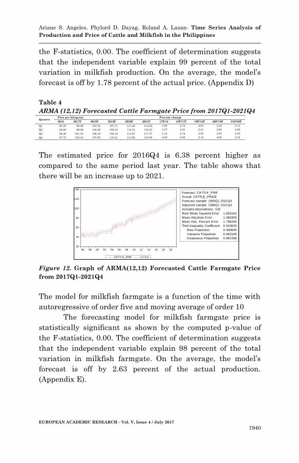
the F-statistics, 0.00. The coefficient of determination suggests
that the independent variable explain 99 percent of the total
variation in milkfish production. On the average, the model’s
forecast is off by 1.78 percent of the actual price. (Appendix D)
Table 4
ARMA (12,12) Forecasted Cattle Farmgate Price from 2017Q1-2021Q4
Quarter Peso per kilogram Percent change
2016 2017F 2018F 2019F 2020F 2021F 17F/16 18F/17F 19F/18F 20F/19F 21F/20F
Q1 93.35 98.86 103.55 107.71 111.46 114.94 5.90 4.74 4.03 3.48 3.13
Q2 94.88 99.98 104.86 108.54 112.54 116.24 5.37 4.88 3.51 3.68 3.29
Q3 96.40 101.35 106.16 109.43 113.67 117.57 5.14 4.74 3.08 3.88 3.43
Q4 97.72 102.43 107.00 110.41 114.82 118.88 4.82 4.46 3.18 4.00 3.53
The estimated price for 2016Q4 is 6.38 percent higher as
compared to the same period last year. The table shows that
there will be an increase up to 2021.
Figure 12. Graph of ARMA(12,12) Forecasted Cattle Farmgate Price
from 2017Q1-2021Q4
The model for milkfish farmgate is a function of the time with
autoregressive of order five and moving average of order 10
The forecasting model for milkfish farmgate price is
statistically significant as shown by the computed p-value of
the F-statistics, 0.00. The coefficient of determination suggests
that the independent variable explain 98 percent of the total
variation in milkfish farmgate. On the average, the model’s
forecast is off by 2.63 percent of the actual production.
(Appendix E).

Ariane S. Angeles, Phylord D. Dayag, Roland A. Lazan- Time Series Analysis of
Production and Price of Cattle and Milkfish in the Philippines
EUROPEAN ACADEMIC RESEARCH - Vol. V, Issue 4 / July 2017
1941
Table 5
ARMA (5,10) Forecasted Fish Farmgate Price from 2017Q1-2021Q4
Quarte
r
Peso per kilogram Percent change
2016 2017F 2018F 2019F 2020F 2021F
17F/1
6
18F/17
F
19F/18
F
20F/19
F
21F/20
F
Q1
128.65
125.73
131.27
136.17
139.33
142.42 (2.27) 4.40 3.73 2.32 2.22
Q2
127.83
127.35
132.70
138.07
140.52
143.37 (0.37) 4.20 4.05 1.77 2.02
Q3
124.07
128.26
134.17
138.82
141.15
144.03 3.38 4.61 3.47 1.68 2.04
Q4
125.50
128.81
135.11
139.40
141.73
144.69 2.64 4.89 3.18 1.68 2.08
The estimated price for 2016Q4 is 0.83 percent lower as
compared to the same period last year. The table shows that
there will be an increase up to 2021.
Figure 13. Graph of ARMA(5,10) Forecasted Milkfish Production from
2017Q1-2021Q4
V. Summary, Conclusion and Recommendation
5.1 Summary and Conclusion
This study forecasted the production and farmgate price of
Cattle and Milkfish in the Philippines Using Autoregressinve
Integrated Moving Average (ARIMA) and Autoregressive
Moving Average (ARMA). Models with lowest Akaike
Information Critera (AIC) and Bayesian information criterion
(BIC) was considered as best fitted model. Best fitted model
obtained for Cattle production is ARIMA(4,1,2) and
ARIMA(12,1,12) for Milkfish Production. ARMA(12,12) and
ARMA(5,10) is the best fitted model respectively for cattle and
milkfish farmgate prices. The results from these models are
then used to make predictions of the future values of the
production and price of Cattle and Milkfish from 2017-2021.
40,000
60,000
80,000
100,000
120,000
140,000
05 06 07 08 09 10 11 12 13 14 15 16 17 18 19 20 21
MILKFISHF ± 2 S.E.
Forecast: MILKFISHF
Actual: MILKFISH
Forecast sample: 2002Q1 2021Q4
Adjusted sample: 2005Q2 2021Q4
Included observations: 66
Root Mean Squared Error 3443.945
Mean Absolute Error 2245.160
Mean Abs. Percent Error 2.627047
Theil Inequality Coefficient 0.017832
Bias Proportion 0.007616
Variance Proportion 0.001124
Covariance Proportion 0.991260
Ariane S. Angeles, Phylord D. Dayag, Roland A. Lazan- Time Series Analysis of
Production and Price of Cattle and Milkfish in the Philippines
EUROPEAN ACADEMIC RESEARCH - Vol. V, Issue 4 / July 2017
1942
The trend in the production and price of cattle and milkfish in
the country has an increasing movement over the years. The
trend of the forecast follows the trend of the actual value.
The forecasting ability of the model for a five year forecast is
shown to be relatively good.
5.2 Recommendation
Policy makers can use the forecasted production and farmgate
prices to impost acts that would benefit both producers and
consumers. And also, this study can be relate to further studies
where in production is related like consumption, import and
exports of milkfish and cattle in the Philippines. Forecasting
production and price can be done along with other variables like
consumption, imports, exports through Vector Autoregressive
Analysis; and also, Granger causality to know if the variables
can granger cause each other.
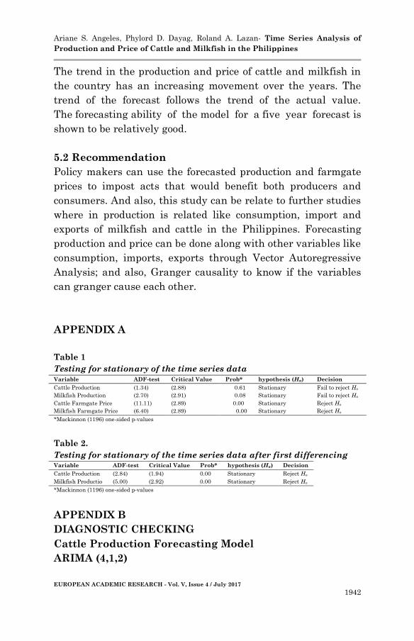
APPENDIX A
Table 1
Testing for stationary of the time series data Variable ADF-test Critical Value Prob* hypothesis (Ha) Decision
Cattle Production (1.34) (2.88) 0.61 Stationary Fail to reject Ho
Milkfish Production (2.70) (2.91) 0.08 Stationary Fail to reject Ho
Cattle Farmgate Price (11.11) (2.89) 0.00 Stationary Reject Ho
Milkfish Farmgate Price (6.40) (2.89) 0.00 Stationary Reject Ho
*Mackinnon (1196) one-sided p-values
Table 2.
Testing for stationary of the time series data after first differencing Variable ADF-test Critical Value Prob* hypothesis (Ha) Decision
Cattle Production (2.84) (1.94) 0.00 Stationary Reject Ho
Milkfish Productio (5.00) (2.92) 0.00 Stationary Reject Ho
*Mackinnon (1196) one-sided p-values
APPENDIX B
DIAGNOSTIC CHECKING
Cattle Production Forecasting Model
ARIMA (4,1,2)

Ariane S. Angeles, Phylord D. Dayag, Roland A. Lazan- Time Series Analysis of
Production and Price of Cattle and Milkfish in the Philippines
EUROPEAN ACADEMIC RESEARCH - Vol. V, Issue 4 / July 2017
1943
0
5
10
15
20
25
-0.10 -0.05 0.00 0.05 0.10
Series: ResidualsSample 1981Q1 2016Q4Observations 144
Mean 0.000496Median -0.001624Maximum 0.107267Minimum -0.115781Std. Dev. 0.039422Skewness -0.063524Kurtosis 3.687790
Jarque-Bera 2.935175Probability 0.230481
Table 3
Significance of the variable in ARIMA (4,1,2)
Variable Coefficient Std. Error t-Statistic Prob.
AR(3) -0.0894 0.03391 -2.6374 0.0093
AR(4) 0.93655 0.03374 27.7575 0
MA(1) -0.6417 0.083134 -7.7183 0
MA(2) 0.23541 0.083767 2.81031 0.0057
R-squared 0.94756 Mean dependent var 0.33035
Adjusted R-squared 0.94642 S.D. dependent var 7.37643
S.E. of regression 1.70739 Akaike info criterion 3.93538
Sum squared resid 405.209 Schwarz criterion 4.01826
Log likelihood -277.38 Hannan-Quinn criter. 3.96906
Durbin-Watson stat 2.0564
Figure 1 Correlogram for ARIMA (4,1,2)
Figure 2. Normality Test for ARIMA(4,1,2)

Ariane S. Angeles, Phylord D. Dayag, Roland A. Lazan- Time Series Analysis of
Production and Price of Cattle and Milkfish in the Philippines
EUROPEAN ACADEMIC RESEARCH - Vol. V, Issue 4 / July 2017
1944
Table 3
Breusch-Godfrey Serial Correlation LM Test for ARIMA(4,1,2)
F-statistic 1.03372 Prob. F(4,135) 0.3923
Obs*R-squared 3.93553 Prob. Chi-Square(4) 0.4148
Table 4
Heteroskedasticity Test for ARIMA(4,1,2)
F-statistic 1.87666 Prob. F(10,132) 0.0538
Obs*R-squared 17.7999 Prob. Chi-Square(10) 0.0584
Scaled explained SS 24.0153 Prob. Chi-Square(10) 0.0076
ARIMA (1,1,7)
Table 5
Significance of the Variable in ARIMA (1,1,7)
Variable Coefficient Std. Error t-Statistic Prob.
D(CATTLE(-4)) 0.95467 0.033189 28.7648 0
AR(1) -0.5995 0.068972 -8.6914 0
MA(7) -0.1536 0.084647 -1.8142 0.0718
R-squared 0.94631 Mean dependent var 0.33894
Adjusted R-squared 0.94553 S.D. dependent var 7.40183
S.E. of regression 1.72743 Akaike info criterion 3.95205
Sum squared resid 414.78 Schwarz criterion 4.0145
Log likelihood -277.6 Hannan-Quinn criter. 3.97743
Durbin-Watson stat 2.13873
Figure 3. Correlogram for ARIMA(1,1,7)

Ariane S. Angeles, Phylord D. Dayag, Roland A. Lazan- Time Series Analysis of
Production and Price of Cattle and Milkfish in the Philippines
EUROPEAN ACADEMIC RESEARCH - Vol. V, Issue 4 / July 2017
1945
0
5
10
15
20
25
-6 -5 -4 -3 -2 -1 0 1 2 3 4 5
Series: ResidualsSample 1981Q3 2016Q4Observations 142
Mean 0.040362Median 0.096918Maximum 5.472553Minimum -5.643124Std. Dev. 1.714661Skewness -0.279936Kurtosis 4.183083
Jarque-Bera 10.13608Probability 0.006295
Figure 4 Normality Test for ARIMA(1,1,7)
Table 6
Breusch-Godfrey Serial Correlation LM Test for ARIMA (1,1,7)
F-statistic 0.53908 Prob. F(12,127) 0.8856
Obs*R-squared 6.80698 Prob. Chi-Square(12) 0.8701
Table 7
Heteroskedasticity Tes t for ARIMA (1,1,7)
F-statistic 1.62366 Prob. F(6,135) 0.1452
Obs*R-squared 9.55739 Prob. Chi-Square(6) 0.1446
Scaled explained SS 14.448 Prob. Chi-Square(6) 0.025
ARIMA (12,1,4)
Table 8
Significance of the Variable for ARIMA(12,1,4) Variable Coefficient Std. Error t-Statistic Prob.
AR(3) -0.3076 0.056661 -5.4288 0
AR(12) 0.75097 0.063713 11.7869 0
MA(4) 0.46079 0.059007 7.80907 0
MA(1) -0.539 0.058311 -9.2433 0
R-squared 0.91093 Mean dependent var 0.3817
Adjusted R-squared 0.90889 S.D. dependent var 7.55824
S.E. of regression 2.28137 Akaike info criterion 4.51661
Sum squared resid 681.806 Schwarz criterion 4.60269
Log likelihood -300.87 Hannan-Quinn criter. 4.55159
Durbin-Watson stat 2.37758

Ariane S. Angeles, Phylord D. Dayag, Roland A. Lazan- Time Series Analysis of
Production and Price of Cattle and Milkfish in the Philippines
EUROPEAN ACADEMIC RESEARCH - Vol. V, Issue 4 / July 2017
1946
Figure 5 Correlogram for ARIMA(12,1,4)
Figure 6. Normality Test for ARIMA(12,1,4)
Table 9
Breusch-Godfrey Serial Correlation LM Test for ARIMA(12,1,4)
F-statistic 2.35692 Prob. F(3,128) 0.0749
Obs*R-squared 5.7068 Prob. Chi-Square(3) 0.1268
Table 10
Heteroskedasticity Test for ARIMA(12,1,4)
F-statistic 0.23273 Prob. F(10,124) 0.9925
Obs*R-squared 2.48703 Prob. Chi-Square(10) 0.9911
Scaled explained SS 3.21805 Prob. Chi-Square(10) 0.9758
APPENDIX C
DIAGNOSTIC CHECKING
Milkfish Production Forecasting Model
ARIMA(12,1,4)

Ariane S. Angeles, Phylord D. Dayag, Roland A. Lazan- Time Series Analysis of
Production and Price of Cattle and Milkfish in the Philippines
EUROPEAN ACADEMIC RESEARCH - Vol. V, Issue 4 / July 2017
1947
Table 11
Significance of the Variable for ARIMA(12,1,4)
Variable Coefficient Std. Error t-Statistic Prob.
AR(12) 1.0644 0.068533 15.5312 0
MA(4) 0.726604 0.075313 9.64779 0
MA(3) -0.27331 0.092037 -2.9696 0.0048
R-squared 0.950412 Mean dependent var 1369.9
Adjusted R-squared 0.948158 S.D. dependent var 23655.5
S.E. of regression 5386.08 Akaike info criterion 20.0827
Sum squared resid 1.28E+09 Schwarz criterion 20.2008
Log likelihood -468.944 Hannan-Quinn criter. 20.1272
Durbin-Watson stat 2.539958
Correlogram
Figure 7 Correlogram for ARIMA(12,1,4)
Normality
Figure 8 Normality Test for ARIMA(12,1,4)
0
2
4
6
8
10
-10000 -5000 0 5000 10000
Series: ResidualsSample 2005Q2 2016Q4Observations 47
Mean -155.2979Median -25.56304Maximum 10639.15Minimum -11238.93Std. Dev. 5265.351Skewness -0.069502Kurtosis 2.347294
Jarque-Bera 0.872138Probability 0.646573

Ariane S. Angeles, Phylord D. Dayag, Roland A. Lazan- Time Series Analysis of
Production and Price of Cattle and Milkfish in the Philippines
EUROPEAN ACADEMIC RESEARCH - Vol. V, Issue 4 / July 2017
1948
Table 12
Breusch-Godfrey Serial Correlation LM Test for ARIMA(12,1,4)
F-statistic 1.26381 Prob. F(12,32) 0.2863
Obs*R-squared 15.0841 Prob. Chi-Square(12) 0.2369
Table 13
Heteroskedasticity Test for ARIMA(12,1,4)
F-statistic 1.07118 Prob. F(5,41) 0.3904
Obs*R-squared 5.43034 Prob. Chi-Square(5) 0.3656
Scaled explained SS 3.22848 Prob. Chi-Square(5) 0.6648
ARIMA(4,1,8)
Table 14
Significance of the Variable for ARIMA(4,1,8)
Variable Coefficient Std. Error t-Statistic Prob.
AR(4) 1.026566 0.02506 40.9605 0
MA(8) -0.53395 0.03732 -14.306 0
MA(1) -0.73575 0.05509 -13.356 0
MA(6) 0.306916 0.05741 5.34623 0
R-squared 0.967535 Mean dependent var 1247.86
Adjusted R-squared 0.965626 S.D. dependent var 22500.6
S.E. of regression 4.17E+03 Akaike info criterion 19.58
Sum squared resid 8.88E+08 Schwarz criterion 19.726
Log likelihood -534.449 Hannan-Quinn criter. 19.6364
Durbin-Watson stat 2.06812
Figure 9 Correlogram for ARIMA(4,1,8)

Ariane S. Angeles, Phylord D. Dayag, Roland A. Lazan- Time Series Analysis of
Production and Price of Cattle and Milkfish in the Philippines
EUROPEAN ACADEMIC RESEARCH - Vol. V, Issue 4 / July 2017
1949
0
1
2
3
4
5
6
7
8
9
-12000 -8000 -4000 0 4000 8000 12000
Series: ResidualsSample 2003Q2 2016Q4Observations 55
Mean -312.6338Median -882.4591Maximum 12073.37Minimum -11827.90Std. Dev. 4041.845Skewness 0.183270Kurtosis 4.215670
Jarque-Bera 3.694635Probability 0.157659
Figure 10. Normality Test for ARIMA(4,1,8)
Table 15
Breusch-Godfrey Serial Correlation LM Test for ARIMA(4,1,8)
F-statistic 0.63984 Prob. F(8,43) 0.7399
Obs*R-squared 5.55119 Prob. Chi-Square(8) 0.6974
Table 16
Heteroskedasticity Test for ARIMA(4,1,8)
F-statistic 0.42891 Prob. F(10,44) 0.9245
Obs*R-squared 4.88512 Prob. Chi-Square(10) 0.8987
Scaled explained SS 6.60382 Prob. Chi-Square(10) 0.7622
ARIMA(12,1,12)
Table 17
Significance of the Variable for ARIMA(12,1,12)
Variable Coefficient Std. Error t-Statistic Prob.
AR(12) 1.101436 0.02624 41.9775 0
AR(5) 0.053676 0.02038 2.63368 0.0116
MA(12) -0.96346 0.02727 -35.325 0
R-squared 0.969589 Mean dependent var 1369.9
Adjusted R-squared 0.968206 S.D. dependent var 23655.5
S.E. of regression 4217.955 Akaike info criterion 19.5938
Sum squared resid 7.83E+08 Schwarz criterion 19.7119
Log likelihood -457.454 Hannan-Quinn criter. 19.6382
Durbin-Watson stat 2.508435

Ariane S. Angeles, Phylord D. Dayag, Roland A. Lazan- Time Series Analysis of
Production and Price of Cattle and Milkfish in the Philippines
EUROPEAN ACADEMIC RESEARCH - Vol. V, Issue 4 / July 2017
1950
Figure 11. Correlogram for ARIMA(12,1,12)
Figure 12. Normality Test for ARIMA(12,1,12)
Table 18
Breusch-Godfrey Serial Correlation LM Test for ARIMA(12,1,12)
F-statistic 1.55545 Prob. F(12,32) 0.1557
Obs*R-squared 16.9941 Prob. Chi-Square(12) 0.1498
Table 19
Heteroskedasticity Test for ARIMA(12,1,12)
F-statistic 1.14646 Prob. F(6,40) 0.3539
Obs*R-squared 6.89653 Prob. Chi-Square(6) 0.3305
Scaled explained SS 4.83319 Prob. Chi-Square(6) 0.5654
APPENDIX D
DIAGNOSTIC CHECKING
Cattle Farmgate Forecasting Model
ARMA(12,12)
0
1
2
3
4
5
6
7
8
-8000 -4000 0 4000 8000
Series: ResidualsSample 2005Q2 2016Q4Observations 47
Mean 422.0410Median -200.7272Maximum 9478.418Minimum -8433.999Std. Dev. 4103.123Skewness 0.215883Kurtosis 2.501018
Jarque-Bera 0.852668Probability 0.652898

Ariane S. Angeles, Phylord D. Dayag, Roland A. Lazan- Time Series Analysis of
Production and Price of Cattle and Milkfish in the Philippines
EUROPEAN ACADEMIC RESEARCH - Vol. V, Issue 4 / July 2017
1951
Table 20
Significance of the variables for ARMA(12,12)
Variable Coefficient Std. Error t-Statistic Prob.
AR(1) 0.912911 0.045447 20.08732 0
AR(12) 0.107883 0.050763 2.125219 0.0366
MA(12) -0.245729 0.109326 -2.247674 0.0273
R-squared 0.989641 Mean dependent var 66.4812
Adjusted R-squared 0.989385 S.D. dependent var 18.0514
S.E. of regression 1.859803 Akaike info criterion 4.11388
Sum squared resid 280.1683 Schwarz criterion 4.20069
Log likelihood -169.7829 Hannan-Quinn criter. 4.14878
Durbin-Watson stat 2.2249
Figure 13. Correlogram for ARMA(12,12)
Figure 14. Normality Test for ARMA(12,12)
0
4
8
12
16
20
-5 -4 -3 -2 -1 0 1 2 3 4 5
Series: ResidualsSample 1996Q1 2016Q4Observations 84
Mean -0.037569Median -0.118036Maximum 5.402158Minimum -5.195348Std. Dev. 1.836870Skewness 0.034716Kurtosis 4.201698
Jarque-Bera 5.071148Probability 0.079216

Ariane S. Angeles, Phylord D. Dayag, Roland A. Lazan- Time Series Analysis of
Production and Price of Cattle and Milkfish in the Philippines
EUROPEAN ACADEMIC RESEARCH - Vol. V, Issue 4 / July 2017
1952
Table 21
Breusch-Godfrey Serial Correlation LM Test for ARMA(12,12)
F-statistic 1.514734 Prob. F(12,69) 0.14
Obs*R-squared 17.48628 Prob. Chi-Square(12) 0.1322
Table 22
Heteroskedasticity Test ARMA(12,12)
F-statistic 1.19165 Prob. F(6,77) 0.3197
Obs*R-squared 7.13719 Prob. Chi-Square(6) 0.3083
Scaled explained SS 10.6112 Prob. Chi-Square(6) 0.1012
ARMA(6,8)
Table 23
Significance of the Variables for ARMA(6,8)
Variable Coefficient Std. Error t-Statistic Prob.
AR(1) 0.852597 0.055499 15.36251 0
AR(6) 0.677031 0.084893 7.97515 0
AR(5) -0.50793 0.105513 -4.813908 0
MA(5) 0.797081 0.056214 14.17938 0
MA(8) -0.17508 0.061314 -2.855386 0.0054
R-squared 0.990411 Mean dependent var 64.90578
Adjusted R-squared 0.989959 S.D. dependent var 18.43432
S.E. of regression 1.847167 Akaike info criterion 4.119136
Sum squared resid 290.0222 Schwarz criterion 4.258014
Log likelihood -180.361 Hannan-Quinn criter. 4.17514
Durbin-Watson stat 2.161403
Figure 15. Correlogram for ARMA(6,8)
Ariane S. Angeles, Phylord D. Dayag, Roland A. Lazan- Time Series Analysis of
Production and Price of Cattle and Milkfish in the Philippines
EUROPEAN ACADEMIC RESEARCH - Vol. V, Issue 4 / July 2017
1953
Figure 16. Normality Test for ARMA(6,8)
Table 24
Breusch-Godfrey Serial Correlation LM Test for ARIMA(6,8)
F-statistic 0.769411 Prob. F(8,77) 0.6306
Obs*R-squared 6.661916 Prob. Chi-Square(8) 0.5735
Table 25
Heteroskedasticity Test for ARIMA(6,8)
F-statistic 0.80325 Prob. F(15,74) 0.6704
Obs*R-squared 12.602 Prob. Chi-Square(15) 0.633
Scaled explained SS 16.1155 Prob. Chi-Square(15) 0.3744
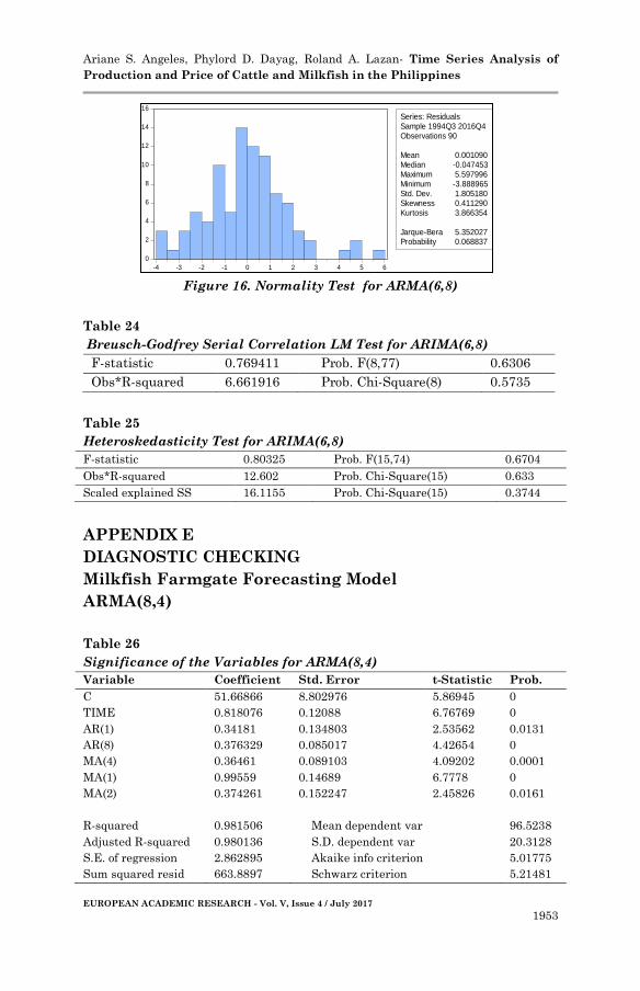
APPENDIX E
DIAGNOSTIC CHECKING
Milkfish Farmgate Forecasting Model
ARMA(8,4)
Table 26
Significance of the Variables for ARMA(8,4)
Variable Coefficient Std. Error t-Statistic Prob.
C 51.66866 8.802976 5.86945 0
TIME 0.818076 0.12088 6.76769 0
AR(1) 0.34181 0.134803 2.53562 0.0131
AR(8) 0.376329 0.085017 4.42654 0
MA(4) 0.36461 0.089103 4.09202 0.0001
MA(1) 0.99559 0.14689 6.7778 0
MA(2) 0.374261 0.152247 2.45826 0.0161
R-squared 0.981506 Mean dependent var 96.5238
Adjusted R-squared 0.980136 S.D. dependent var 20.3128
S.E. of regression 2.862895 Akaike info criterion 5.01775
Sum squared resid 663.8897 Schwarz criterion 5.21481
0
2
4
6
8
10
12
14
16
-4 -3 -2 -1 0 1 2 3 4 5 6
Series: ResidualsSample 1994Q3 2016Q4Observations 90
Mean 0.001090Median -0.047453Maximum 5.597996Minimum -3.888965Std. Dev. 1.805180Skewness 0.411290Kurtosis 3.866354
Jarque-Bera 5.352027Probability 0.068837
Ariane S. Angeles, Phylord D. Dayag, Roland A. Lazan- Time Series Analysis of
Production and Price of Cattle and Milkfish in the Philippines
EUROPEAN ACADEMIC RESEARCH - Vol. V, Issue 4 / July 2017
1954
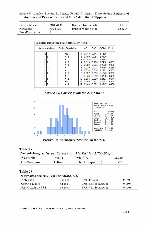
Log likelihood -213.7809 Hannan-Quinn criter. 5.09714
F-statistic 716.4528 Durbin-Watson stat 1.83214
Prob(F-statistic) 0
Figure 17. Correlogram for ARMA(8,4)
Figure 18. Normality Test for ARMA(8,4)
Table 27
Breusch-Godfrey Serial Correlation LM Test for ARMA(8,4)
F-statistic 1.36604 Prob. F(8,73) 0.2259
Obs*R-squared 11.4575 Prob. Chi-Square(8) 0.1771
Table 28
Heteroskedasticity Test for ARMA(8,4)
F-statistic 1.38535 Prob. F(35,52) 0.1407
Obs*R-squared 42.462 Prob. Chi-Square(35) 0.1804
Scaled explained SS 38.6091 Prob. Chi-Square(35) 0.3098
0
2
4
6
8
10
-8 -6 -4 -2 0 2 4 6
Series: ResidualsSample 1995Q1 2016Q4Observations 88
Mean -0.009648Median 0.007145Maximum 7.384757Minimum -7.520817Std. Dev. 2.762394Skewness 0.001457Kurtosis 3.146444
Jarque-Bera 0.078666Probability 0.961431

Ariane S. Angeles, Phylord D. Dayag, Roland A. Lazan- Time Series Analysis of
Production and Price of Cattle and Milkfish in the Philippines
EUROPEAN ACADEMIC RESEARCH - Vol. V, Issue 4 / July 2017
1955
ARMA(5,10)
Table 29
Significance of the Variables for ARMA(5,10)
Variable Coefficient Std. Error t-Statistic Prob.
C 54.3969 5.17394 10.5136 0
TIME 0.78336 0.08335 9.39885 0
AR(1) 0.71 0.07868 9.02438 0
AR(4) 0.50146 0.09646 5.19839 0
AR(5) -0.3814 0.09728 -3.9212 0.0002
MA(1) 0.53556 0.04955 10.8082 0
MA(10) -0.4641 0.04779 -9.711 0
R-squared 0.98233 Mean dependent var 95.5685
Adjusted R-squared 0.98107 S.D. dependent var 20.639
S.E. of regression 2.83991 Akaike info criterion 4.99923
Sum squared resid 677.469 Schwarz criterion 5.19237
Log likelihood -220.46 Hannan-Quinn criter. 5.07715
F-statistic 778.243 Durbin-Watson stat 1.91955
Prob(F-statistic) 0
Figure 19. Correlogram of ARMA(5,10)
Figure 20. Normality Test of ARMA(5,10)
0
2
4
6
8
10
12
14
-6 -4 -2 0 2 4 6 8
Series: ResidualsSample 1994Q2 2016Q4Observations 91
Mean 0.063624Median -0.263186Maximum 8.261244Minimum -6.125723Std. Dev. 2.742872Skewness 0.542646Kurtosis 3.605343
Jarque-Bera 5.855470Probability 0.053518
Ariane S. Angeles, Phylord D. Dayag, Roland A. Lazan- Time Series Analysis of
Production and Price of Cattle and Milkfish in the Philippines
EUROPEAN ACADEMIC RESEARCH - Vol. V, Issue 4 / July 2017
1956
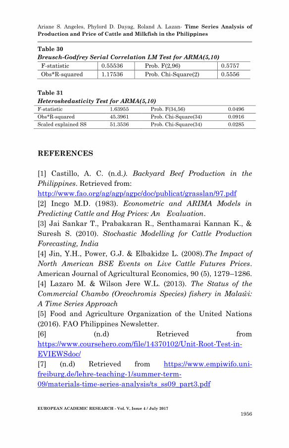
Table 30
Breusch-Godfrey Serial Correlation LM Test for ARMA(5,10)
F-statistic 0.55536 Prob. F(2,96) 0.5757
Obs*R-squared 1.17536 Prob. Chi-Square(2) 0.5556
Table 31
Heteroskedasticity Test for ARMA(5,10) F-statistic 1.63955 Prob. F(34,56) 0.0496
Obs*R-squared 45.3961 Prob. Chi-Square(34) 0.0916
Scaled explained SS 51.3536 Prob. Chi-Square(34) 0.0285
REFERENCES
[1] Castillo, A. C. (n.d.). Backyard Beef Production in the
Philippines. Retrieved from:
http://www.fao.org/ag/agp/agpc/doc/publicat/grasslan/97.pdf
[2] Incgo M.D. (1983). Econometric and ARIMA Models in
Predicting Cattle and Hog Prices: An Evaluation.
[3] Jai Sankar T., Prabakaran R., Senthamarai Kannan K., &
Suresh S. (2010). Stochastic Modelling for Cattle Production
Forecasting, India
[4] Jin, Y.H., Power, G.J. & Elbakidze L. (2008).The Impact of
North American BSE Events on Live Cattle Futures Prices.
American Journal of Agricultural Economics, 90 (5), 1279–1286.
[4] Lazaro M. & Wilson Jere W.L. (2013). The Status of the
Commercial Chambo (Oreochromis Species) fishery in Malaŵi:
A Time Series Approach
[5] Food and Agriculture Organization of the United Nations
(2016). FAO Philippines Newsletter.
[6] (n.d) Retrieved from
https://www.coursehero.com/file/14370102/Unit-Root-Test-in-
EVIEWSdoc/
[7] (n.d) Retrieved from https://www.empiwifo.uni-
freiburg.de/lehre-teaching-1/summer-term-
09/materials-time-series-analysis/ts_ss09_part3.pdf

Ariane S. Angeles, Phylord D. Dayag, Roland A. Lazan- Time Series Analysis of
Production and Price of Cattle and Milkfish in the Philippines
EUROPEAN ACADEMIC RESEARCH - Vol. V, Issue 4 / July 2017
1957
[8] (n.d) Retrieved from
https://en.wikipedia.org/wiki/Correlogram
[9] (n.d) Retrieved from
https://en.wikipedia.org/wiki/Jarque%E2%80%93Bera_test
[10] (n.d) Retrieved from
https://onlinecourses.science.psu.edu/stat501/node/366
[11] (n.d) Retrieved from
http://www.statsmakemecry.com/smmctheblog/confusing-stats-
terms-
explained-heteroscedasticity-heteroske.html
[12] Retrieved from https://coolstatsblog.com/2013/08/14/using-
aic-to-test-arima-models-2/
[13] Retrieved from https://www.otexts.org/fpp/8/6
[14] Retrieved from
https://en.wikipedia.org/wiki/Bayesian_information_criterion
[15] Retrieved from http://www.mixph.com/the-philippines-beef-
cattle-industry/
[16] Retrieved from
http://www.pcaarrd.dost.gov.ph/home/momentum/milkfish/
[17] Retrieved from http://business.inquirer.net/211357/ph-
among-worlds-fastest-growing-meat-
consumers-say-experts
[18] Retrieved from
https://en.wikipedia.org/wiki/Ljung%E2%80%93Box_test
[19] Retrieved from
http://ejournalofsciences.org/archive/vol3no6/vol3no6_4.pdf
[20] Retrieved from
http://www.alliedacademies.org/articles/crop-yield-prediction-
using-time-series-models.pdf
[21] Retrieved from
https://pdfs.semanticscholar.org/4d3d/632eaea7b1c43d73572051
dc8a2c1f1d 2708.pdf?_ga=2.234174875.423889231.1495318098-
235198729.1495318091 [20]
[22] Retrieved from
http://www.ams.sunysb.edu/~zhu/ams586/UnitRoot_ADF.pdf

Ariane S. Angeles, Phylord D. Dayag, Roland A. Lazan- Time Series Analysis of
Production and Price of Cattle and Milkfish in the Philippines
EUROPEAN ACADEMIC RESEARCH - Vol. V, Issue 4 / July 2017
1958
[23] Retrieved from
https://en.wikipedia.org/wiki/Ljung%E2%80%93Box_test
[24] Retrieved from
http://www.etsii.upm.es/ingor/estadistica/Carol/TSAtema10pett
en.pdf
[25] Retrieved from
http://webspace.ship.edu/pgmarr/Geo441/Lectures/Lec%205%20
-%20Normality%20Testing.pdf