title solar and lunar hydromagnetic tides in the …

RIGHT:

URL:

CITATION:

AUTHOR(S):

ISSUE DATE:

TITLE:

SOLAR AND LUNARHYDROMAGNETIC TIDES IN THEEARTH'S MAGNETOSPHERE

MAEDA, Hiroshi

MAEDA, Hiroshi. SOLAR AND LUNAR HYDROMAGNETIC TIDES IN THEEARTH'S MAGNETOSPHERE.

1970-12

http://hdl.handle.net/2433/178588

Special Contributions, Geophysical Institute, Kyoto University, No. 10, 1970, 1-11

SOLAR AND LUNAR HYDROMAGNETIC TIDES IN THE EARTH'S MAGNETOSPHERE

By

Hiroshi MAEDA

(Received November 9, 1970)

Abstract

Hydromagnetic tidal oscillations in the magnetosphere of the Earth are obtained

on the basis of the electrostatic fields in the dynamo region as deduced from

solar and lunar geomagnetic variations. It is found that the magnetosphere

expands during the daytime and contracts during the night for the solar tides,

and expands around Oh and 12h lunar time and contracts around 6h and ISh lunar

time for the lunar tides. Effects of these tidal motions on the distribution of plasma density are then estimated and discussed.

I. Introduction

Tidal phenomena are common and basic in the field of geophysics. They

are understood as a deformation in different areas of the Earth caused by the

gravitation of other celestial bodies (mainly the Moon and the Sun), and

consist of ocean tides in the hydrosphere, earth tides in the lithosphere, and atmospheric tides in the atmosphere.

In the case of atmospheric tides, pressure measurements on the ground

reveal substantial oscillations with periods of 12 and 24 solar hours, together

with a weak component with a period of 12 lunar hours. The lunar component

can be generated only by gravitational forces, while the 24 hr solar component

is now believed to be due to thermal processes. The 12 hr solar component

could be generated by either or both of these processes. Thus, the solar

atmospheric tides may not properly be called tides but oscillations in their basic definition.

Tidal oscillations in the upper atmosphere are fairly different from those

in the lower atmosphere, because the atmospheric gas is very tenuous and is

ionized in different degree at different heights. They were first a source of

interest in relation to the dynamo theory of geomagnetic variations, and it is

now accepted that in the dynamo region !the E region of the ionosphere) the

solar 24 hr oscillations are excited by thermal processes, and that the solar

and lunar 12 hr oscillations are produced by leakage of tidal energy from

2 H. MAEDA

below. In addition to these oscillations, a circulation may occur in the dynamo

region, in association with a nonuniform distribution of gas pressure. The

resultant winds can induce an electric current in the dynamo region of the

ionosphere.

The electric current thus induced sets up an electrostatic field, because it

should be divergence-free. Such a field in the dynamo region may transfer

itself to the upper ionosphere and magnetosphere along the highly conducting

lines of geomagnetic force, and drive the ionized gas into motion. This problem

was first considered by Martyn (1955J in interpreting observed drift motions

and tidal phenomena in the F2 region of the ionosphere, and has been discussed

by a number of researchers thereafter. Extension of this problem to the mag-

"' 90°

60.

30° liJ I=> ::J 1- o· 1-<I: _J

3o'

·~[ 90 s

/ / \ / "' \ /p /! -- 'f-. ' I'! '[ , - [\ ~ L J. 1

L ~ ./ I ~

~-+--- ----:;--2--+- __.;.__:..__ .J ~--/---+-!- (

-"-+---+---!--+--- ' /'

~---- ~ ~ .----+-----------.--";-·--T--T- l----t-+--.--+- --~ ----\;-- -;\--£ +-----"----\----\-~ .______.....__ _,________" --'1;-- . ....... ... ' ~ _.,.:__.

- \'- - ---------"<--~ i

---+--t~ 'j_ t / '/ \' """~ './ ,. ... / 'I T \.-' /'

I \ ~ I

00 04 08 12 20

SOLAR TIME

LUNAR TIME

E -"' :::: 0 ,.

...

...J

"' (J

"' ~ 0 « « <(

E .... :::: 0 >

...

...J c u "' :It 0 a: « <(

Fig. 1. Distribution of the solar and lunar electrostatic fields in the dynamo region, obtained by the dynamo theory of geomagnetic variations.

HYDROMAGNETIC TIDES IN THE MAGNETOSPHERE 3

netosphere was initiated by Gold (1959), and associated plasma motions were called hyd romagnetic tides by Hines (1963).

The purpose of this paper is to estimate in some detail the solar and lunar

hydromagnetic tides in the magnetosphere, and to discuss their effects on the distribution of the plasma density.

2. Electrostatic fields in the dynamo region

The electrostatic fields associated with the dynamo currents which are

responsible for the solar and lunar daily geomagnetic viriations are estimated

by solving the dynamo equation, and several attempts for obtaining solutions

have been made. Most of these were made for a two-dimensional model of

the dynamo current layer; i. e., it was assumed that no vertical current flow

ed, and no height change existed in the wind velocity and the electric field.

Such a model seems to be adequate as a first approximation, because of the

fact that the effective layer of the dynamo current is as thin as might be

expected from the vertical distribution of the electrical conductivity, and also from rocket observations of the magnetic field at ionospheric heights.

Worldwide distributions of the electrostatic fields obtained by such a treat

ment are shown in Fig. 1 for the solar (Maeda (1955)) and lunar (Maeda and

Fujiwara (1967)) cases, where the solar field is based on the data obtained

during the Second Polar Year (at sunspot minimum), whereas the lunar field

is considered to be for a moderate sunspot activity because lunar effects can

be estimated by averaging over many years. It is therefore to be noted that

the magnitude of these fields may be somewhat changed with sunspot activity.

3. Transfer of electrostatic fields

Following the suggestion of Martyn (1955) and Dagg (1957) concerning

electrostatic coupling between the dynamo region and the F region of the

ionosphere, Farley (1959, 1960, 1961) and Spreiter and Briggs (1961 a, 1961 b)

considered this problem quantitatively. Although there is a slight difference

between these two sets of treatments, the results show that a significant coupling

between these two regions can occur at all latitudes, especially for a field

having a large horizontal scale. It was also found that the attenuation of

electrostatic fields with height from the dynamo region was less in middle and

high latitudes than in equatorial regions, and less for nighttime conditions than

for daytime conditions. It was further suggested that a significant coupling would occur between magnetically conjugate points of the F region.

On the other hand, the conduction of electrostatic fields from the outer

magnetosphere to the ionosphere via the geomagnetic field lines was studied

4 H. MAEDA

by Reid [1965], and it was concluded that the attenuation would be slight for a field component with wavelength greater than about 10 km.

Thus, all these results show that electrostatic fields are transferred, without

appreciable attenuation in amplitude, from the dynamo region to the upper

ionosphere and magnetosphere along the geomagnetic field lines. This means

that the geomagnetic lines of force can approximately be considered to be

electric equipotential lines, so that the solar and lunar electrostatic fields in

the dynamo region will be mapped into the magnetosphere along the field lines.

The potential distributions mapped on the equatorial plane in such a manner

are showiJ. in Fig. 2 for the solar field (left) and the lunar field (right). This

mapping was made for a dipole field, so that the regions beyond L~5 might be deformed by the effect of the solar wind.

SOLAR TIME LUNAR TIM(

12•

Fig. 2. Distribution of the solar and lunar electrostatic potentials mapped on the equatorial plane of the magnetosphere.

4. Hydromagnetic tides in the magnetosphere

It has been shown by Maeda [1959] that above about 150 km the mean

motion of ionized gases is mainly ' determined by the electrodynamic force

rather than the collisional force: This result has been examined by other

researchers, and is now generally accepted. This being so, the motions of ions and electrons are the same and they satisfy the equation

E+vxH=O, (1)

where V=Vt=V,, or

v=(ExH)/Hz. (2)

Combining this with the electromagnetic equation


an a(= -curl E, (3)

we have an ar=curl (vxH). (4)

This implies that the magnetic lines of force are constrained to move with the

material.

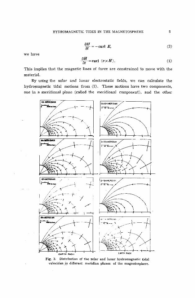
By using the solar and lunar electrostatic fields, we can calculate the

hydromagnetic tidal motions from (2). These motions have two components,

one in a meridional plane (called the meridional component), and the other

Oh MERIDIAN ............... 0 IOiil&fMC --~----J...

//~ / ~

IZ

112h II[IIIIDIAN / ' .___.___. ' 0 100•1 ... ,' ___ 1

/ ------ \ / -·~

/ I

I <---r--- f

' EARTH RADII

I

I

--+

Ohi12hl MERIDIAN

EARTH RADII

Fig. 3. Distribution of the solar and lunar hydromagnetic tidal velocities in different meridian planes of the magnetosphere.

6 H. MAEDA

normal to the meridional plane (called the zonal component). Of these com

ponents, only the meridional component plays an important part in tidal

oscillations, because it produces a compression and expansion of the magneto

spheric plasma as is shown in Fig. 3. The hydromagnetic tides in the equatorial

plane associated with this meridional component are shown in Fig. 4. It is

seen from the figures that an expansion occurs in the daytime and a contraction

at night for the solar tides, and that an expansion occurs around Oh and 12h

lunar time and a contraction around 6h and 18h lunar time for the lunar

tides.

50[ 50

40 40

J 30~ 0

w u z c:( 20 f-(/)

a u ii: f-z w u 010 w <..?

8

& 0 12 18 24

6 0 ~~~7-~-~~~-L-L------

6 12 18 24 SOLAR TIME (hr) LUNAR TIME (hr)

Fig. 4. Solar and lunar hydromagnetic tides in the equatorial plane of the magnetosphere.

5. Density variation associated with tidal motions

4

The plasma density in a static magnetosphere may be changed by tidal

motions. This would be understood by Alfven's concept of the frozen in fields. By using the equation

div H=O,

the hydromagnetic equation ( 4) becomes

88f =(H·grad) v-(v·grad) H-Hdivv.

On the other hand, the equation of continuity

~( +div (pv) =0,

(5)

(6)

(7)


gives

1 8p _ v · gra«!___e_ divv=---p-- at p (8)

By combining (6) and (8) we have

(9)

This equation, derived by Wal€m (1946J, implies that if two infinitely close

field particles are on the same line of force at any time, then they will always

be on that line of force, so that the total mass of plasma contained in a

magnetic tube of force remains constant as the tube is carried about.

Application of this result to the magnetosphere (Gold (1959J) shows that if

a tube of force moves from RA to R,. in its equatorial distance then the density

will change from PA to p,. such that

p,. ( R,. )-• p;= RA ' (10)

because the volume of the tube changes as (RH RA)•.

In order to estimate the density variation associated with tidal motions,

we need to know the density distribution in a static magnetosphere. Several

attempts have been made for obtaining the density distribution from whistler

id5

":' 10 E c..>

>-1-en z

•

I.JJ 010 3

z 0 0:: 1-u I.JJ ....J I.JJ 10 2

I

(<'\'. -6.\ ~'. ~\ o' q;\

>?o \ .

\~ (" ·!\. 1?£. :'>\. ~ \" 1l \·.

'' .

' '·.N· \ . 1\N~. \ · .

. ·~

ALTITUDE (km)

Fig. 5. Different models of the density distribution in a static magnetosphere, where Naoc(RE 'R)+', N,oc(R:gR)+a exp(3RE/R), and Nsoc(RE/R)+<.

8 H. MAEDA

data. Liemohn and Scarf (1964J analysed fiftyseven nose whistler traces to test the validity of model magnetospheric electron distributions. The models used by them were

(11)

where Ki2 is a numerical factor, and F 1 =1, F2=exp (3RE/ R) , Fa= (RE/R)+3,

F4 = (RE/R )+3 exp (3RE/ R ), and F 5= (RE/RC00))+3 exp ( -3RE/RC00) +3RE/ R ). In these factors, F1 is the simplest, F2 is suggested by evaporation theories, Fa is a gyrofrequency model, and F4 and Fs have been discussed by Johnson (1959, 1962J . For the sake of comparison, we add one more ; F6 = (RE1 R )+4_ It is clear that Fs=F3 on the equatorial plane, so that we examined the three models Fa, F. and Fs, because Liemohn and Scarf (1964J concluded that the densities derived from the whistler data were in very good agreement with Fa and F. ,

L • 5.0 I h • 25480kml

0.5

2.0 L • 5 .0 (h • 25480kml

I 0~-·-=--·- · -- · .,_...-.:::----=

0 .5

2.0 L•3.0fh•l2740kml

1.0~;::::;>-~=--===,_...-..:_~. --= 0 .5

o20 L • 2 .0 (h= 6370kml z ;: 1 oi=...--~~-~=~-""""'"=~-..-==d-

05

2 .0 L • l.47(h=3000kml

r.ob= ... · --~~--~~------..J

0 .5

2 .0 L•1.16(h•IOOOkml . -·~ _ .... ·""" ...... , 2·0 L • 1.16 (h•IOOOkm l

1.0

0 .5

0

1.0 ·- . ..... ...... . .... . - · - ·-·- - ·- -·-·-·-· 0.5

6 12 24 0 6 12 18 SOLAR TIME (hr) LUNAR TIME (hr)

Fig. 6. Density variation caused by the solar and lunar tidal oscillations in the equatorial plane of the magnetosphere, where the full lines are for N,, the dotted lines for N a, the broken lines for No, and the chains for the extended Chapman layer.

24


in fair agreement with F 5, and in poor agreement with F, and Fz. These distributions are used at great heights above 2000 km, while below this level a Chapman layer extending from the ionospheric F region is employed (see Fig. 5) .

The density variations caused by the solar and lunar hydromagnetic tides are calculated on the basis of the magnetospheric models obtained above, and are shown in Fig. 6, where the full lines are for F~, the dotted lines for F3, the broken lines for F 6, and the chains for a Chapman layer. It is found that the effect of tidal motions is remarkable in the topside ionosphere below 2000 km. Above about 2000 km, the density becomes high during the nighttime and low during the daytime for the solar tides, whereas its maximum is around 6h and 18h lunar time and minimum around 0h and 12h lunar time for the lunar tides. The results for different models are such that no effect can be seen for F 6 as expected from equation (10) , and the effect is larger for F~ than for F3.

6. Discussion

Before discussing our results, it is important to examine the processes by which the present results are derived. The electrostatic fields in the dynamo region have been obtained by regarding the ionospheric currents as flowing in an infinitesimally thin shell in the E region, so that the following two assumptions have been made in the mathematical treatment: (1) no vertical currents, and (2) height-independent winds and electric fields.

Assumption (1) has been criticized by Dougherty (1963], suggesting a significant contribution of field-aligned currents between geomagnetically conjugate points. Nishida and Fukushima (1959] considered the effect of vertical currents in a layer of limited thickness, and pointed out a possibility of the modification of electrostatic fields by this effect. On the other hand, recent rocket observations (see Kochanski (1964] for example) have shown that the wind velocity in the dynamo region is considerably changed with height, so that assumption (2) may not be made.

Even if the above effects are ignored in a first approximation, there still remains a question about the uniqueness of the solution for the dynamo equation. This problem has recently been discussed by Mohlmann and Wagner (1970], and they have pointed out that the velocity field derived from the current density alone represents only one part of the total velocity field in the ionosphere, suggesting a significant effect in estimating the electrostatic fields.

Next, we have to discuss the conduction of electrostatic fields from the dynamo region to the magnetosphere. Although our estimates have been made

10 H. MAEDA

on the assumption that the geomagnetic field lines can be regarded as electric equipotentials, several restrictions may be imposed on this assumption. One possibility is the existence of turbulence in the magnetosphere, which results in an electric field along the field lines. Mapping relationships in the presence of such a parallel field have been discussed by Reid (1965] and recently by Mozer (1970].

Another possibility has been pointed out by Alfven and Faltbammer (1963] in relation to the plasma density in the magnetosphere. Outer regions of the magnetosphere seem to be collision-free, so that an individual electron obeys the equation of motion

dvn E m ----;[{- = e 11 • (12)

The potential difference between the ionosphere (C) and the equator (A) in this case has been estimated by Alfven and Falthammer as follows:

Vo- v .. = _r_:- 1_( J:V; II w._~_-W.ulf;_L) lei W;u +Well A,

(13)

where r=Ho/ H 1, and W 11 =mv 11 2j 2 and W _1_ =mv_~_2j2 with the i~dices e and i referring to electrons and ions. Thus the concept of equipotentials is not applicable in general, and we need to know how the particle population is injected.

In spite of these restrictions, hydromagnetic tidal motions as obtained in this paper would exist in the magnetosphere, especially in the inner magnetosphere on quiet days. Their effect on the distribution of the plasma density would also be real. However, we have ignored here the density discontinuity at the magnetopause as was found by Carpenter (1966]. If it is taken into account, interesting tidal phenomena may be expected at the magnetopause.

Note added in proof

We ignored in this paper the effects of the zonal component and the corotation. It should be noted, therefore, that if these effects are taken into account, the phases of tidal oscillations and density variations might be different from those shown in Figs. 3, 4, and 6. Results of calculation in which all the effects are taken into consideration will be published elsewhere.

Acknowledgements

This study was initiated while the author worked at the Goddard Institute for Space Studies, NASA, in New York as a senior research associate of NSF / NRC. Most of the numerical analyses were made on a FACOM 230-60 computer at the Data Processing Center of Kyoto University.


References

Alfven, H. and C.-G. Falthammer, 1963; Cosmical Electrodynamics, 2nd ed., Oxford University Press.

Carpenter, D. L., 1966; Whistler studies of the plasma pause in the magnetosphere (1), ].

Geophys. Res., 71. 693-709. Dagg, M., 1957; The origin of the ionospheric irregularities responsible for radio star

scintillations and spread F (II), J. Atmosph. Terr. Phys., 11, 139-150. Dougherty, J.P., 1963; Some comments on dynamo theory, J. Geophys. Res., 68, 2383-

2384. Farley, D. T., Jr., 1959; A theory of electrostatic fields in a horizontally stratified iono

sphere subject to a vertical magnetic field, J. Geophys. Res., 64, 1225-1233. Farley, D. T., Jr., 1960; A theory of electrostatic fields in the ionosphere at nonpolar

geomagnetic latitudes, J. Geophys. Res., 65, 869-877. Farley, D. T., Jr., 1961; Discussion of paper by John R. Spreiter and Benjamin R. Briggs

on "Theory of electrostatic fields in the ionosphere at polar and middle geomagnetic latitudes", J. Geophys. Res., 66, 3956-3957.

Gold, T., 1959; Motions in the magnetosphere of the earth, J. Geophys. Res., 64, 1219-1224.

Hines, C. 0., 1963; Upper atmosphere in motion, Quart. J. Roy. Meteorol. Soc., 89, 1-42. Johnson, F. S .. 1959; The structure of the outer atmosphere including the ion distribution

above the F 2 maximum, Lockheed Tech. Rept., LMSD 49719. Johnson, F. S., 1962; Physics of the distribution of ionized particles in the exosphere,

Proc. Symp. on Electron Density Profiles, ed. by Malhlm, Mcmillan Co., New York. Kochanski. A., 1964; Atmospheric motions from sodium cloud drifts, J. Geophys. Res.,

69, 3651-3662. Liemohn, H. B. and F. L. Scarf, 1964; Whistler determination of electron energy and

density distributions in the magnetosphere, J. Geophys. Res., 69, 883-904. Maeda, H., 1955; Horizontal wind systems in the ionospheric E region deduced from the

dynamo theory of the geomagnetic Sq variation, Part 1, J. Geomag. Geoelec., 7. 121-132.

Maeda, H., 1959 ; Horizontal winds and ionization drifts in the ionosphere, Rept. Ionosph. Space Res. Japan, 13, 79-90.

Maeda, H. and M. Fujiwara, 1967; Lunar ionospheric winds deduced from the dynamo theory of geomagnetic variations, J. Atmosph. Terr. Phys., 29, 917-936.

Martyn, D. F., 1955; Interpretation of observed F2 winds as ionization drifts associated with the magnetic variations, in Physics of the Ionosphere, The Physical Society, London, 163-165.

Mohlmann, D. and C.-U. Wagner, 1970; On the determination of ionospheric velocity fields from geomagnetic Sq variations, J. Atmosph. Terr. Phys., 32, 445-447.

Mozer, F. S., 1970; Electric field mapping in the ionosphere at the equatorial plane, Planet. Space Sci., 18, 259-263.

Nishida, A. and N. Fukushima, 1959; Three-dimensional consideration for current system of geomagnetic variations, II, Rept. Ionosph. Space Res. Japan, 13, 237-282.

Reid, G. C., 1965 ; Ionospheric effects of electrostatic fields generated in the outer magnetosphere, Radio Science, 69 D. 827-837.

Spreiter, J. R. and B. R. Briggs, 1961 a ; Theory of electrostatic fields in the ionosphere at polar and middle geomagnetic latitudes, J. Geophys. Res., 66, 1731-1744.

Spreiter, J. R. and B. R. Briggs, 1961 b; Theory of electrostatic fields in the ionosphere at equatorial latitudes, J. Geophys. Res., 66, 2345-2354.

Walen, C., 1946; On the distribution of the solar general magnetic field, Arkiv Mat., 33 A. No. 18.

title solar and lunar hydromagnetic tides in the …

Documents