HYDROMAGNETIC COUETTE FLOW BETWEEN TWOVERTICAL SEMI-INFINITE PERMEABLE PLATES

COLLINS OWUOR OTIENO

MASTER OF SCIENCE(Applied Mathematics)

JOMO KENYATTA UNIVERSITY OFAGRICULTURE AND TECHNOLOGY

2021

Hydromagnetic Couette flow between two vertical semi-infinite permeable

plates

Collins Owuor Otieno

A Thesis Submitted in Partial Fulfillment of the Requirements for

the Degree of Master of Science in Applied Mathematics of the Jomo

Kenyatta University of Agriculture and Technology

2021

DECLARATION

This thesis is my original work and has not been submitted for a degree award in any otherUniversity.

Signature........................................ Date.........................................

Collins Owuor Otieno

This thesis has been submitted for examination with our approval as University Supervisors.

Signature........................................ Date.........................................

Prof. Mathew N. Kinyanjui, PhD

JKUAT, Kenya

Signature........................................ Date.........................................

Dr. Roy Kiogora, PhD

JKUAT, Kenya

ii

DEDICATION

This Thesis is dedicated to my parents Mr. George Otieno and Mrs. Edwina Otieno, my uncle Dr.Ochieng’ Raduma, my siblings Valary Opiyo, Brenda Ogutu and Fiona Awuor.

iii

ACKNOWLEDGMENT

I am highly greatful to my supervisors Prof. M.N. Kinyanjui and Dr. Roy Kiogora of JomoKenyatta University of Agriculture and Technology from the Department of Pure and AppliedMathematics for their advice and support in ensuring that this study is a success. Their inspiration,support and knowledge I gathered from them helped me to come up with relevant problem of study.They have ensured that am on the right track in every step.My appreciation goes to my parents, Mr. George Otieno and Mrs. Edwina Otieno, my uncle Dr.Ochieng’ Raduma and family for their encouragement and financial support in my studies.I also acknowledge the support of my friends Dr. Edward Richard, Mr. Kenneth Muya, Mr.Jared Ogutu, Vellah Onkoba and my course mates Amos, Paul and Chepkonga for their continuedencouragement.Finally, I thank the Almighty God for the gift of life and good health He has given me throughoutthis course.

iv

TABLE OF CONTENTS

DECLARATION . . . . . . . . . . . . . . . . . . . . . . . . . . . . . . . . . . . . . . . . ii

DEDICATION . . . . . . . . . . . . . . . . . . . . . . . . . . . . . . . . . . . . . . . . . iii

ACKNOWLEDGMENT . . . . . . . . . . . . . . . . . . . . . . . . . . . . . . . . . . . . iv

TABLE OF CONTENTS . . . . . . . . . . . . . . . . . . . . . . . . . . . . . . . . . . . v

LIST OF FIGURES . . . . . . . . . . . . . . . . . . . . . . . . . . . . . . . . . . . . . . vii

LIST OF APPENDICES . . . . . . . . . . . . . . . . . . . . . . . . . . . . . . . . . . . ix

ABBREVIATIONS . . . . . . . . . . . . . . . . . . . . . . . . . . . . . . . . . . . . . . x

NOMENCLATURE . . . . . . . . . . . . . . . . . . . . . . . . . . . . . . . . . . . . . . xi

GREEK SYMBOLS . . . . . . . . . . . . . . . . . . . . . . . . . . . . . . . . . . . . . . xii

ABSTRACT . . . . . . . . . . . . . . . . . . . . . . . . . . . . . . . . . . . . . . . . . . xiii

CHAPTER ONE:. . . . . . . . . . . . . . . . . . . . . . . . . . . . . . . . . . . . . . . . . 1

INTRODUCTION . . . . . . . . . . . . . . . . . . . . . . . . . . . . . . . . . . . . . . . 11.1 Background of the study . . . . . . . . . . . . . . . . . . . . . . . . . . . . . . . 1

1.1.1 Background knowledge . . . . . . . . . . . . . . . . . . . . . . . . . . . . 11.1.2 Definition of key terms . . . . . . . . . . . . . . . . . . . . . . . . . . . . 1

1.1.2.1 Fluid . . . . . . . . . . . . . . . . . . . . . . . . . . . . . . . . 11.1.2.2 Couette flow . . . . . . . . . . . . . . . . . . . . . . . . . . . . 21.1.2.3 Steady and Unsteady flow . . . . . . . . . . . . . . . . . . . . . 21.1.2.4 Laminar flow . . . . . . . . . . . . . . . . . . . . . . . . . . . . 21.1.2.5 Lorentz force . . . . . . . . . . . . . . . . . . . . . . . . . . . . 21.1.2.6 Viscosity . . . . . . . . . . . . . . . . . . . . . . . . . . . . . . 31.1.2.7 Porous medium . . . . . . . . . . . . . . . . . . . . . . . . . . . 31.1.2.8 Natural convection . . . . . . . . . . . . . . . . . . . . . . . . . 31.1.2.9 Buoyancy . . . . . . . . . . . . . . . . . . . . . . . . . . . . . . 3

1.1.3 Non-Dimensionalization . . . . . . . . . . . . . . . . . . . . . . . . . . . 41.1.3.1 Reynolds number (Re) . . . . . . . . . . . . . . . . . . . . . . . 4

v

1.1.3.2 Prandtl Number (Pr) . . . . . . . . . . . . . . . . . . . . . . . . 41.1.3.3 The Eckert number (EC) . . . . . . . . . . . . . . . . . . . . . . 51.1.3.4 Joules heating parameter (R) . . . . . . . . . . . . . . . . . . . . 51.1.3.5 Magnetic parameter (M) . . . . . . . . . . . . . . . . . . . . . . 6

1.2 Statement of the Problem . . . . . . . . . . . . . . . . . . . . . . . . . . . . . . . 61.3 Justification of the study . . . . . . . . . . . . . . . . . . . . . . . . . . . . . . . 71.4 Objective of the study . . . . . . . . . . . . . . . . . . . . . . . . . . . . . . . . . 7

1.4.1 General objective . . . . . . . . . . . . . . . . . . . . . . . . . . . . . . . 71.4.2 Specific objectives . . . . . . . . . . . . . . . . . . . . . . . . . . . . . . 8

CHAPTER TWO:. . . . . . . . . . . . . . . . . . . . . . . . . . . . . . . . . . . . . . . . . 9

LITERATURE REVIEW . . . . . . . . . . . . . . . . . . . . . . . . . . . . . . . . . . . 9

CHAPTER THREE:. . . . . . . . . . . . . . . . . . . . . . . . . . . . . . . . . . . . . . . . . 13

METHODOLOGY . . . . . . . . . . . . . . . . . . . . . . . . . . . . . . . . . . . . . . 133.1 Model Formulstion . . . . . . . . . . . . . . . . . . . . . . . . . . . . . . . . . . 133.2 Assumptions . . . . . . . . . . . . . . . . . . . . . . . . . . . . . . . . . . . . . . 133.3 Governing Equations . . . . . . . . . . . . . . . . . . . . . . . . . . . . . . . . . 14

3.3.1 Equation of continuity . . . . . . . . . . . . . . . . . . . . . . . . . . . . 143.3.2 Electromagnetic equations . . . . . . . . . . . . . . . . . . . . . . . . . . 15

3.3.2.1 Gauss’ Law for Magnetism . . . . . . . . . . . . . . . . . . . . 153.3.2.2 Faraday’s law of induction . . . . . . . . . . . . . . . . . . . . . 163.3.2.3 Ampere’s Law . . . . . . . . . . . . . . . . . . . . . . . . . . . 16

3.3.3 Equation of Momentum . . . . . . . . . . . . . . . . . . . . . . . . . . . . 163.3.4 Energy Equation . . . . . . . . . . . . . . . . . . . . . . . . . . . . . . . 20

3.4 Non-Dimensionalization . . . . . . . . . . . . . . . . . . . . . . . . . . . . . . . 223.4.1 Initial and boundary conditions . . . . . . . . . . . . . . . . . . . . . . . 223.4.2 Governing equations . . . . . . . . . . . . . . . . . . . . . . . . . . . . . 23

3.5 Method of Solution . . . . . . . . . . . . . . . . . . . . . . . . . . . . . . . . . . 253.5.1 Outline of method of solution . . . . . . . . . . . . . . . . . . . . . . . . . 253.5.2 Advantages of using finite difference method . . . . . . . . . . . . . . . . 30

CHAPTER FOUR:. . . . . . . . . . . . . . . . . . . . . . . . . . . . . . . . . . . . . . . . . 31

vi

RESULTS AND DISCUSSIONS . . . . . . . . . . . . . . . . . . . . . . . . . . . . . . . 314.1 Introduction . . . . . . . . . . . . . . . . . . . . . . . . . . . . . . . . . . . . . . 314.2 Results and Discussions . . . . . . . . . . . . . . . . . . . . . . . . . . . . . . . . 31

4.2.1 A graph showing the effects of varying Reynolds number on primary velocity 314.2.2 A graph showing the effects of varying Magnetic number on primary velocity 314.2.3 A graph showing the effects of varying permeability parameter on primary

velocity . . . . . . . . . . . . . . . . . . . . . . . . . . . . . . . . . . . . 324.2.4 A graph showing the effects of varying Reynolds number on secondary

velocity, Re . . . . . . . . . . . . . . . . . . . . . . . . . . . . . . . . . . 334.2.5 A graph showing the effects of varying permeability parameter on

secondary velocity . . . . . . . . . . . . . . . . . . . . . . . . . . . . . . 344.2.6 A graph showing the effects of varying Prandtl number on Temperature

profile . . . . . . . . . . . . . . . . . . . . . . . . . . . . . . . . . . . . . 354.2.7 A graph showing the effects of varying Reynolds number on Temperature

profile . . . . . . . . . . . . . . . . . . . . . . . . . . . . . . . . . . . . . 364.2.8 A graph showing the effects of varying Eckert number on Temperature profile 374.2.9 A graph showing the effects of varying Joule heating parameter (R)

Temperature profile . . . . . . . . . . . . . . . . . . . . . . . . . . . . . . 384.3 Validation of Results . . . . . . . . . . . . . . . . . . . . . . . . . . . . . . . . . 39

CHAPTER FIVE:. . . . . . . . . . . . . . . . . . . . . . . . . . . . . . . . . . . . . . . . . 41

CONCLUSION AND RECOMENDATIONS . . . . . . . . . . . . . . . . . . . . . . . . 415.1 Introduction . . . . . . . . . . . . . . . . . . . . . . . . . . . . . . . . . . . . . . 415.2 Conclusions . . . . . . . . . . . . . . . . . . . . . . . . . . . . . . . . . . . . . . 415.3 Recommendations . . . . . . . . . . . . . . . . . . . . . . . . . . . . . . . . . . . 42

REFERENCES . . . . . . . . . . . . . . . . . . . . . . . . . . . . . . . . . . . . . . . . . 43

APPENDICES . . . . . . . . . . . . . . . . . . . . . . . . . . . . . . . . . . . . . . . . . 46Published Article . . . . . . . . . . . . . . . . . . . . . . . . . . . . . . . . . . . . . . 46MATLAB Codes . . . . . . . . . . . . . . . . . . . . . . . . . . . . . . . . . . . . . . 47

vii

LIST OF FIGURES

Figure 3.1: Geometry of the flow . . . . . . . . . . . . . . . . . . . . . . . . . . . . 13Figure 3.2: Illustration of the mesh . . . . . . . . . . . . . . . . . . . . . . . . . . . 26

Figure 4.1: Velocity profiles for varied values of the Reynolds number, Re. . . . . . 32Figure 4.2: Velocity profiles for varied values of the Magnetic number, M. . . . . . . 33Figure 4.3: Velocity profiles for varied values of the X number. . . . . . . . . . . . . 34Figure 4.4: Velocity profiles for varied values of the Reynolds number, Re. . . . . . 35Figure 4.5: Velocity profiles for varied values of the x number. . . . . . . . . . . . . 36Figure 4.6: Temperature profiles for varied values of the Pr number. . . . . . . . . . 37Figure 4.7: Temperature profiles for varied values of the Re number. . . . . . . . . . 38Figure 4.8: Temperature profiles for varied values of the Ec number. . . . . . . . . . 39Figure 4.9: Temperature profiles for varied values of the R number. . . . . . . . . . 40

viii

LIST OF APPENDICES

Appendix I: Published Article ...................................................................................46Appendix II: MATLAB Codes .................................................................................47

ix

LIST OF ABBREVIATIONS

MHD Magnetohydrodynamics

PDE Partial Differential Equations

FDM Finite Difference Method

FEM Finite Element Method

FVM Finite Volume Method

MATLAB Matrix Laboratory

x

LIST OF NOMENCLATURES

SYMBOLS MEANING

−→B Magnetic field strength (Wbm−2)

Bo Magnetic flux density (Wbm−2)

g Acceleration due to gravity (ms−2)

−→H Magnetic field intensity (Am−1)

−→J Current density (AM−2)

Re Reynolds number

p Pressure force (Nm−2)

x∗,y∗, t∗, Dimensionless cartesian coordinates

−→Fi Body forces tensor (N)

−→Vi Velocity tensor (ms−1)

X j Space tensor

−→Fr Electromagnetic force (N)

Pr Prandtl number

Ha Hartman number

Qo Heat generation constant (Wm3)

Cp Specific heat at a constant pressure (JKg−1k−1)

T Temperature (K)

r,θ ,z Cylindrical coordinates

xi

LIST OF GREEK SYMBOLS

SYMBOLS MEANING

µ Viscosity(Kgm−1s−1)

ρ Fluid density (Kgm−3)

η Dynamic viscosity (Kgm−1s−1)

ε Emissivity of black body

σi j Normal stresses (Nm−2)

τi j Shear stresses (Nm−2)

σ Electrical conductivity (Ω−1m−1)

µe Magnetic permeability (Hm−1)

∇ Gradient Operator

xii

ABSTRACT

In the present study, a hydromagnetic Couette flow between two vertical semi-infinite permeableplates with uniform injection/suction while considering Joule heating has been investigated. Theplate where injection takes place is stationary while the other plate moves with a time dependantvelocity in the x-direction. Also, a constant magnetic field is applied perpendicular to thestationary plate. The study involves an electrically conducting fluid flow that is incompressibe,viscous and unsteady. The equations that govern the flow which are continuity equation,momentum equation and energy equation were formed and then non-dimensionalised. Due to thenon-linear nature of the equations, they cannot be solved analytically and therefore, the method ofsolution was the finite difference numerical technique because it is more stable and accurate. Theresults were analyzed and presented graphically. It was established that various non-dimensionalparameters such as Joule Heating parameter, Prandtl Number, Eckert Number and othernon-dimensional parameters had effects on temperature and velocity profiles which werediscussed into details. The effects of varying these parameters led to either increase, decrease orno effect on flow variables. The findings of this study shall be applied in areas such as the designof cooling systems with liquid metal, electrostatic precipitation, purification of crude oil,petroleum industry, aerodynamic heating, polymer technology, accelerators and many others.

xiii

CHAPTER ONE

INTRODUCTION

1.1 Background of the study

1.1.1 Background knowledge

MHD Couette flow of an electrically conducting fluid is one of the problems which has received

considerable attention due to its varied and wide applications in areas of Geophysics, Astrophysics

and fluid engineering fields. The word magneto-hydrodynamic (MHD) is derived from; Magneto

which refers to magnetic field while hydro refers liquid and dynamics refers to the motion of a body

under influence of forces. Therefore, hydrodynamics refers to the study of fluid that is in motion

and the forces that affects the motion while MHD is the study of the dynamics of an electrically

conducting fluid in the presence of magnetic field.

Some application areas of interest for this study are in designing of cooling systems with liquid

metals, electrostatic precipitation, purification of crude oil, polymer technology among others. The

key terms used in the study are defined and discussed into details in the subsection that follows.

1.1.2 Definition of key terms

1.1.2.1 Fluid

A fluid refers to any substance that undergoes continuous deformation when acted upon by an

external force. Fluids are classified as liquids or gases. Anderson (2007) from his definition of

fluid explained that molecules in a fluid are held together by intermolecular forces such that the

fluid tends to possess a volume but no definite shape.

1

1.1.2.2 Couette flow

Couette flow is a laminar flow of a viscous fluid in the space between two plates which are parallel

to each other. One of the plate moves tangetially and the flow is driven by virtue of the viscous drag

force which acts on the fluid but may be additionally be motivated by an applied pressure gradient

in the flow direction. This type of flow is named in honor of Maurice Marie Alfred Couette, a

Professor of Physics in French university of Angers in the late 19th century.

1.1.2.3 Steady and Unsteady flow

Fluid flow can be classified as either steady or unsteady. Steady flow is a flow in which at a

particular fixed point, the fluid flow variables such as pressure and temperature do not change with

respect to time while unsteady flow is one in which the flow variables at a particular fixed point

change with respect to time.

In this study we shall consider unsteady flow scenario.

1.1.2.4 Laminar flow

Laminar flow refers to a flow where there is steady motion of particles of fluid. The fluid flows in

parallel layers with no disruption between them. Velocity and viscosity affects the flow in such a

way that laminar flow occurs at lower velocities, below the threshold at which the flow becomes

turbulent. Turbulent flow is a less orderly flow which results in lateral mixing of fluid layers. The

flow of study is laminar flow

1.1.2.5 Lorentz force

The transverse application of a magnetic field to a flow field induces a current and the interaction

of this current with the magnetic field generates Lorentz force and according to De Andrade and

Pereira (2015), this force opposes the flow and reduces the fluids velocity.

2

1.1.2.6 Viscosity

According to Ahmed (2015), viscosity of a fluid refers to the measure of its resistance to gradual

deformation by shear stress or tensile stress. When the fluid flows through a tube, the particles

which compose the fluid generally move more quickly near the tube’s axis and more slowly near

its walls. Therefore, some stress such as pressure difference between the two ends of the tube is

needed to overcome the friction between particle layers to keep the fluid moving. Ideal fluid or

inviscid fluid is a fluid that has no resistance to shear stress.

1.1.2.7 Porous medium

Porous medium refers to any material with voids or pores. As defined by Steenbrink and Van der

Giessen (2016), porosity or void fraction is the measure of voids in a material. A non-porous

material is one that is not permeable to fluids. Permeability is the measure of the ability of a

porous material to allow fluids to pass through.

1.1.2.8 Natural convection

Free (or natural) convection is the mode of heat transfer in which the flow is as a result of density

gradient created by temperature variation. On the other hand, forced convection occurs when the

flow is caused by some external means.

1.1.2.9 Buoyancy

This is the upward force that is exerted by a fluid and it opposes the weight of a partially or

fully immersed body. It occurs when there is a changes in density of the fluid. A change in

temperature results into a change in density that causes free convection in the fluid. An increase

in fluid temperature causes thermal expansion hence a decrease in fluid density. From Archimedes

principle where upthrust = ρvg, v represents the volume of the fluid displaced, ρ is the fluid density

3

and g is the acceleration due to gravity.

1.1.3 Non-Dimensionalization

This is the partial or full removal of units from an equation involving physical quantities using

substitution of suitable variables.

Under some similar set of conditions, this process aims at ensuring that the results obtained from

a study are applicable to other geometrically similar configurations. This method starts with

selecting a suitable scale against which all dimensions in a given physical model are scaled with

great generality and mathematical simplicity.

The non-dimensional parameters are discussed as follows;

1.1.3.1 Reynolds number (Re)

Reynold’s number is the ratio of inertial forces to viscous forces. It shows the effect on the

flowing fluid when the forces changes. At small Reynolds number, there is large viscous forces

hence a low velocity flowing fluid. When viscous forces are more dorminant than inertial forces

reduces. An increase in Reynold’s number shows an increases in the flowing fluid velocity due to

a reduction of viscous force of the fluid and this may cause the flow to be turbulent.

Reynolds number is given by:

ρU∞Hµ

= Re (1.1.1)

1.1.3.2 Prandtl Number (Pr)

This is the ratio of the viscous diffusion rate to thermal diffusion.As the Prandtl number tends to

one, the velocity boundary layer thickness and the thermal boundary layers are almost of the same

thickness. When the Prandtl number is less than 1, the thermal boundary layer is larger than the

4

velocity boundary layer. For most gaseous substances, the Prandtl number is less than one at

standard temperature and pressure. When the Prandtl number of a fluid is more than one, then the

velocity boundary layer becomes larger than the thermal boundary layer. Prandtl number is

expressed as;

Pr =ρcp

k(1.1.2)

1.1.3.3 The Eckert number (EC)

This is the ratio of the fluid’s kinetic energy to thermal internal energy. It shows the rate at which

the kinetic energy is converted to internal heat energy due to the resistance of the flowing particles

by the viscous forces of the fluid . It is conventionally agreed that when Eckert number is positive,

the fluid have gained heat from the surrounding plate hence a rise in temperature of the fluid and

vice versa implies a loss of heat from the fluid.

Eckert number is expressed as;

Ec =U2

∞

ρcp(Tw−T∞)(1.1.3)

1.1.3.4 Joules heating parameter (R)

This is the heating that occurs when an electric current flows in a conductor which has high

resistance. The flow of electric current in an electrically resistive conductor causes an increase in

temperature in the conductor due to the opposition to the flow of current resulting to more work

done to overcome this forces.

This phenomenon is called joule heating which was named after the scientist Prescott Joule, the

first scientist to establish Joule law which is expressed as;

5

R =B2

oσ µ

ρµρcp(Tw−T∞)(1.1.4)

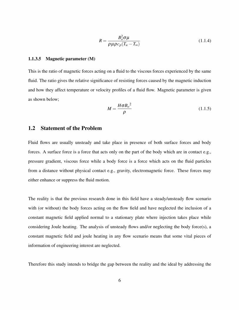
1.1.3.5 Magnetic parameter (M)

This is the ratio of magnetic forces acting on a fluid to the viscous forces experienced by the same

fluid. The ratio gives the relative significance of resisting forces caused by the magnetic induction

and how they affect temperature or velocity profiles of a fluid flow. Magnetic parameter is given

as shown below;

M =HσBo

2

ρ(1.1.5)

1.2 Statement of the Problem

Fluid flows are usually unsteady and take place in presence of both surface forces and body

forces. A surface force is a force that acts only on the part of the body which are in contact e.g.,

pressure gradient, viscous force while a body force is a force which acts on the fluid particles

from a distance without physical contact e.g., gravity, electromagnetic force. These forces may

either enhance or suppress the fluid motion.

The reality is that the previous research done in this field have a steady/unsteady flow scenario

with (or without) the body forces acting on the flow field and have neglected the inclusion of a

constant magnetic field applied normal to a stationary plate where injection takes place while

considering Joule heating. The analysis of unsteady flows and/or neglecting the body force(s), a

constant magnetic field and joule heating in any flow scenario means that some vital pieces of

information of engineering interest are neglected.

Therefore this study intends to bridge the gap between the reality and the ideal by addressing the

6

unsteady hydromagnetic Couette flow between two vertical semi-infinite permeable plates at a

constant magnetic field while considering Joule heating.

Thus the present work is an extension of the work of Job and Gunakala (2016).

1.3 Justification of the study

The research on MHD flows is important to science and engineering fields particularly, the

influence of a magnetic field on an electrically conducting fluid flow that is incompressible,

unsteady and viscous because they are useful in MHD generators, MHD flow meters, heat

exchanger, cooling of nuclear reactors, extraction of iron metal from the ores, extrusion plastics in

the manufacture of rayon and nylon, etc.

There is need to carry out an analysis on hydromagnetic Couette flow between two vertical

semi-infinite plates where a constant magnetic field is applied normally to the main flow while

considering Joule heating since the findings shall be beneficial to engineeers in areas such as

cooling systems where the walls of a channel containing heated fluid are protected from

overheating by passing a cooler fluid through the surface of the channel, in removal of pollutants

from plant discharge streams by absorption, electrostatic precipitation and many other useful

scientific fields.

1.4 Objective of the study

1.4.1 General objective

To study hydromagnetic Couette flow between two vertical semi-infinite permeable plates.

7

1.4.2 Specific objectives

1. To model a hydromagnetic Couette flow between two vertical semi-infinite permeable plates

with uniform injection and suction where a constant magnetic field is applied perpendicuar

to the main flow.

2. To determine the flow variables such as velocity and temperature in profile form.

3. To find the effects of varying the flow parameters such as Joule heating parameter, Prandtl

number, Eckert number on the flow variables such as temperature and velocity.

8

CHAPTER TWO

LITERATURE REVIEW

MHD Couette flow is studied by a number of researchers due to its varied and wide applications in

the areas of fluid engineering and astrophysics. The hydromagnetic flow between porous plates has

many application areas such as flow meters, in underground energy transport among other areas.

Reseachers have studied steady or unsteady flow of an incompressible fluid flow with or without

magnetic field and analyzing different aspects of the problem.

Onyango et al. (2017) analyzed unsteady hydromagnetic Couette flow with magnetic field lines

fixed relative to the moving upper plate and they concluded that magnetic field accelerated the fluid

flow when the pressure gradient is constant. It was also found that viscosity exerted a retarding

influence on the fluid velocity.

Boniface et al. (2014) investigated hydomagnetic steady flow between two infinite parallel

vertical porous plates in the presence of a strong magnetic field applied transverse to the direction

of the flow. It was concluded that that increase in Prandtl number and the suction parameter led to

decrease in fluid temperature. For Grashoff number and magnetic field parameter, their increase

caused an increase in velocity while an increase in the suction velocity led to decreased in the

velocity of the flow. For the magnetic field parameter, its increase led to the increase in the

amplitude of the magnetic field lines.

Seth et al. (2017) discussed effect of induced magnetic field on a flow within a porous channel

when the fluid flow within the channel is induced due to uniformly accelerated motion when one

of the plates starts moving with a time dependent velocity. It was found that magnetic field tends

to decrease the velocitty of the fluid in the plate region whereas it reverses the effect on the

velocity of the fluid in the region away from the plate. Induced magnetic field tends to be

enhanced by chemical reaction in the plate region.

Bodosa and Borkakati (2017) investigated magneto-hydrodynamic Couette flow of an

incompressible, viscous and electrically conducting fluid with a uniform transverse magnetic field

9

acting on the flowing fluid where the fluid flow within the channel is induced due to time

dependent movement of one of the plate. They concluded that velocity distribution increases near

the plates and then decreases very slowly at the central portion between the plates. They also

found out that increase in Prandtl number and Reynolds number led to increase in temperature

distributions.

Onyango et al. (2015) studied the effects of direction of a transverse magnetic field on unsteady

MHD Couette flow with suction and injection. It was concluded that that the direction of the

transverse maagnetic field is important as it leads to increased or decreased velocity of the fluid.

The injection of the fluid led to increased velocity profile while suction led to decreased velocity

of the fluid.

Kinyanjui et al. (2013) analyzed MHD Stokes problem for a vertical infinite plate in dissipative

rotating fluid with Hall current. The results were that increase in Eckert number, magnetic

parameter, rotational parameter led to increase in temperature profile for both free convection

cooling of the plate and free convection heating of the plate. Rajput and Sahu (2016) investigated

unsteady hydromagnetic Couette flow through a vertical channel in the presence of thermal

radiation. They concluded the decrease in velocity profie was brought by an increase in Prandtl

number or magnetic number.

Johana et al. (2018) investigated unsteady free convection incompressible fluid past a

semi-infinite vertical porous plate in the presence of a strong magnetic inclined at an angle α to

the plate with Hall and ion-slip current effects. They concluded that increase in Prandtl number

led to decrease in both primary and secondary velocities of the flow and temperature profiles.

Attia and Ewis (2010) investigated unsteady MHD Couette flow with heat transfer of a

viscoelastic fluid exponential decaying pressure gradient. It was found that the viscoelastic

parameter had a marked effect on the temperature and velocity distributions . Also Attia (2018)

studied unsteady MHD Couette flow of a viscoelastic fluid with heat transfer and found that the

dependence of the temperature on the magnetic field vary with time for all values of the

10

viscoelastic parameter and higher values of the magnetic field.

Muhuri (2018) investigated Couette magneto-hydrodynamics flow with time varying suction and

taking into account the effects of heat and mass transfer.They found that increase in Prandtl

number caused a reduction in fluid temperature which resulted into decrease in fluids velocity.

Mukhopadhyay (2016) investigated the problem where the fluid flow is confined to porous

boundaries with injection and suction. He found that the fluid flow velocity was reduced by

suction and on the other hand it was increased by injection. Injection and magnetic field led to

reduction of the shear stress at the lower plate.

Chauhan and Agrawal (2015) studied the problem of steady hydromagnetic Couette flow of a

highly viscous fluid through a porous channel in the presence of an applied uniform transverse

magnetic field and thermal radiation. It was concluded that decrease in temperatue profile was

due to increased thermal radiation while increase in velocity profiles was due to increase in

magnetic field.

Kim (2018) investigated unsteady MHD convective flow of an incompressible electrially

conducting fluid past an infinite vertical porous plate. The numerical results of the study led to

conclusion that increase in velocity profiles was due to increased Grashoff number while decrease

in velocity profiles was due to increase in Hartman number.

Makinde and Mhone (2019) studied the heat transfer in porous medium in the presence of

transverse magnetic field. They analyzed the effects of the heat source parameter and Nusselt

number and discovered that the effect of increasing porous parameter leads to increase in Nusselt

number.

Jha et al. (2015) investigated unsteady natural convective Couette flow of a viscous fluid through

a vertical channel. It was that increase in time led to decrease in Nusselt number while on the

other had it led to increase in skin friction, temperature and velocity profies. Joseph et al. (2015)

studied unsteady MHD Couette flow between two infinite parallel plates of an inclined magnetic

field with heat transfer. It was found that velocity of the fluid increased due to increased magnetic

11

number. They also concluded that varying Reynolds number affected the temperature of the fluid

flow in that its increase led to increase in the temperature profiles.

Chandran et al (2017) did ananysis of unsteady hydromagnetic Couette flow where magnetic field

lines were fixed relative to the moving upper plate with suction and injection. It was concluded

that the magnetic field, pressure gradient, time and injection have an accelerating influence

whereas suction and viscosity exerts a retarding influence on the fluid flow.

Freidoonimehr et al. (2015) investigated a turbulent incompressible fluid flow past a semi-infinite

vertical plate thati si rotating and an inclined strong magnetic field applied to it. It was concluded

that an increase in primary velocity profile was due to increase in the angle of inclination while a

decrease in the primary velocity profile was due to increase in the Eckert number.

Raptis and Kafousias (2015) analyzed steady convective MHD fluid flow through parallel

semi-infinite plates with constant magnetic field. Hartmann and Prandtl numbers were found to

have a great effect in that a decrease in velocity profiles was as a result of increase in Hartman

number while the decrease in temperature profiles was due to increase in Prandtl number. Job and

Gunakala (2016) studied unsteady magneto-hydrodynamic free convective Couette flow between

two vertical permeable plates in the presence of thermal radiation using Galerkin’s finite method.

They concluded that increase in radiation parameter led to decrease in velocity profiles at small

time but increases them at large time. Both the temperature and velocity profiles increased due to

increase in Prandtl number, Eckert number and Reynolds number.

This study therefore tends to extend the work of Job and Gunakala (2016) with consideration of a

constant magnetic field applied relative to the stationary plate and the other plate where the

suction takes place is on motion and incorporating joule heating.

12

CHAPTER THREE

METHODOLOGY

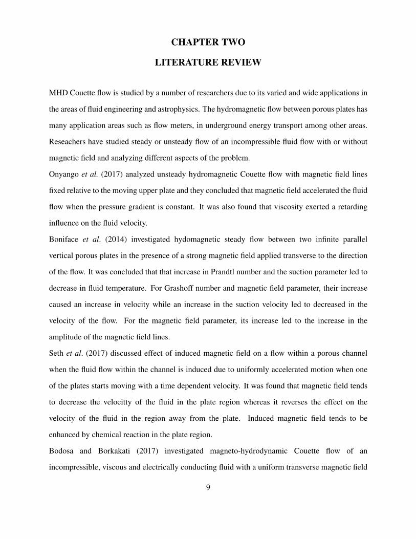
3.1 Model Formulstion

This study considers an incompressible, electrically conducting, viscous and unsteady fluid flow

between two parallel vertical plates along z = 0 and z = h. The plates are of semi-infinite in length

in the x-direction.

Figure 3.1: Geometry of the flow

Initially, at time t = 0, both the plates and fluid are stationary at temperature T0. When t > 0 the

plate along z = h starts moving with time-dependent velocity U0tc in the direction of the main flow

where U0 is a constant and c is a non-negative integer and its temperature rises to T1 while the

other plate located at z = 0 remains stationary with its temperature maintained at T0. A constant

magnetic field B0 is applied normal to the x-axis.

The following assumptions have been used to simplify the problem.

3.2 Assumptions

They are as follows;

13

1. The fluid is incompressible, that is, the density is assumed to be a constant.

2. The fluid flow is two-dimensional.

3. The fluid flow is laminar.

4. There is no chemical reaction.

5. Coefficient of viscosity, electrical conductivity and thermal conductivity are constant.

6. There is negligible force due to electric field since there is no current applied.

3.3 Governing Equations

The fundamentals of fluid dynamics are based on universal laws that govern fluid flows. The

governing equations for this study are continuity equation, momentum equation, equation of energy

and the electromagnetic equations.

3.3.1 Equation of continuity

This equation is derived from the law of conservation of mass. It states that, mass can neither be

created nor destroyed under normal conditions. It is derived by taking a mass balance on the fluid

entering and leaving a volume element in the flow field. The general equation of continuity of a

fluid flow is given :

∂ρ

∂ t+−→∇.(ρ−→q ) = 0 (3.3.1)

where −→q = ui+ v j+wk is the velocity vector in the x,y and z-directions.

In tensor form the equation is:∂ρ

∂ t+

∂

∂xi(ρui) = 0 (3.3.2)

14

Since density is assumed to be constant, then the equation becomes

ρ∂ui

∂xi= 0 (3.3.3)

which in component form is given by

∂u∂x

+∂v∂y

+∂w∂ z

= 0 (3.3.4)

since the flow is in 2-dimensional in z and x direction, the equation becomes

∂u∂x

+∂w∂ z

= 0 (3.3.5)

3.3.2 Electromagnetic equations

These equations give the relationship between the magnetic field intensity−→H , the induction

current density vector−→J , the electric field intensity

−→E , the electric displacement

−→D and the

magnetic induction vector−→B .

The basic electromagnetic equations are as follows:

3.3.2.1 Gauss’ Law for Magnetism

Gauss’ law basically states that all magnetic fields,−→B have field lines that are continuous.

∇.−→B = 0 (3.3.6)

15

3.3.2.2 Faraday’s law of induction

This law states that changes in magnetic fields induces an electric field. It is basically used to

predict how magnetic field interact with electric current to produce electromotive force.

∇×−→E =∂−→B

∂ t(3.3.7)

where−→B = µe

−→H (3.3.8)

3.3.2.3 Ampere’s Law

This Law states that, for any closed loop path, then the product of thr sum of the length elements

and the magnetic field in the direction of the length element is equal to the product of permeability

and the electric current within an enclosed loop.

∇×−→H =−→J (3.3.9)

∇.−→D = ρe (3.3.10)

3.3.3 Equation of Momentum

The equation is derived from the Newton’s second law of motion which requires that the sum of all

the force acting on a control volume must be equal to the rate of change time of fluid momentum

within that control volume.

∂−→q

∂ t+−→q

(−→∇ .−→q

)=− 1

ρ

−→∇ p+

µ

ρ∇

2−→q +−→F i (3.3.11)

16

where−→∇ p represents the pressure gradient of the flow, µ∇2−→q is the viscous force term,

−→F i is the

body forces acting on the flow, −→q(−→

∇ .−→q)

is the convective acceleration that is due to change in

space co-ordinates, ∂−→q

∂ t is the temporal acceleration due to change in time.

The body forces includes magnetic and gravitational forces will be included as follows:

∂−→q

∂ t+−→q

(−→∇ .−→q

)=− 1

ρ

−→∇ p+

µ

ρ∇

2−→q +ρg+~J×~B

ρ(3.3.12)

Lorentz force is given by:

F = ~J×~B (3.3.13)

where

~J = σ(~E +q×~B) (3.3.14)

But ~E = 0 because there is no externally applied electric field, thus

~J = σ(~q×~B) (3.3.15)

now

~J = σ

∣∣∣∣∣∣∣∣∣∣i j k

u v w

Bx By Bz

∣∣∣∣∣∣∣∣∣∣(3.3.16)

the flow is two dimensional and the magnetic fields have been applied perpendicularly to the main

flow.

~J = σ

∣∣∣∣∣∣∣∣∣∣i j k

u 0 w

0 0 Bo

∣∣∣∣∣∣∣∣∣∣=−σuBo j (3.3.17)

17

~F = ~J×~B =

∣∣∣∣∣∣∣∣∣∣i j k

0 −σuBo 0

0 0 Bo

∣∣∣∣∣∣∣∣∣∣=−σuB2

oi (3.3.18)

replacing (3.3.18) in the equation(3.3.12) , it becomes

∂−→q

∂ t+−→q

(−→∇ .−→q

)=− 1

ρ

−→∇ p+

µ

ρ∇

2−→q +ρg− σuB2o

ρ(3.3.19)

When the fluid is heated, the volume of the fluid that is displaced equals to the expanded fluid due

to the thermal expansion. This is given by:

v = β (T −T∞) (3.3.20)

where β is the coefficient of thermal expansion.

where upthrust=Buoyancy:

ρ(β (T −T∞))g = βρg(T −T∞) (3.3.21)

incorporating buoyancy effects in the equation motion given by (3.3.19) becomes

∂−→q

∂ t+−→q

(−→∇ .−→q

)=− 1

ρ

−→∇ p+

µ

ρ∇

2−→q +ρg− σuB2o

ρ+βg(T −T∞) (3.3.22)

The sum of the pressure term in the momentum equation and the gravitational force gives the

porosity term as given in darcy equation:

−∇p+ρg =µ

kpq (3.3.23)

18

putting equation (3.3.23) on (3.3.22) it becomes

∂−→q

∂ t+−→q

(−→∇ .−→q

)=

µ

kpq+

µ

ρ∇

2−→q − σuB2o

ρ+βg(T −T∞) (3.3.24)

since velocity is given in u and w, rewriting (3.3.24) into x and z components the following are

obtained

The momentum equation along the x-axis is given by

∂u∂ t

+~q(−→

∇ .~u)=

µ

kpu+

µ

ρ∇

2u− σuB2o

ρ+βg(T −T∞) (3.3.25)

The momentum equation along the z-axis and using the fact that the magnetic field is parallel to

z-axis, then∂w∂ t

+~q(−→

∇ .~w)=

µ

kpw+µ∇

2w (3.3.26)

but

∇ = i∂

∂x+ k

∂

∂ z(3.3.27)

and

∇2 =

∂ 2

∂x2 +∂ 2

∂ z2 (3.3.28)

Using equations (3.3.27) and (3.3.28) on equation (3.3.25) it becomes

∂u∂ t

+u∂u∂x

+w∂u∂ z

=µ

kpu+

µ

ρ

(∂ 2u∂x2 +

∂ 2u∂ z2

)− σuB2

oρ

+βg(T −T∞) (3.3.29)

Using equations (3.3.27) and (3.3.28) on equation (3.3.26) it becomes

19

∂w∂ t

+u∂w∂x

+w∂w∂ z

=µ

kpw+

µ

ρ

(∂ 2w∂x2 +

∂ 2w∂ z2

)(3.3.30)

Incorporating constant suction and injection in equations (3.3.29) and (3.3.30) becomes

∂u∂ t

+u∂u∂x

+w0∂u∂ z

=µ

kpu+

µ

ρ

(∂ 2u∂x2 +

∂ 2u∂ z2

)− σuB2

oρ

+βg(T −T∞) (3.3.31)

∂w∂ t

+u∂w∂x

+w0∂w∂ z

=µ

kpw+

µ

ρ

(∂ 2w∂x2 +

∂ 2w∂ z2

)(3.3.32)

3.3.4 Energy Equation

This equation is drawn from the principle of conservation of energy which states that energy

neither be created nor destroyed but can only be transformed from one form to the other. The first

law of Thermodynamic states that the amount of heat added to a system equals the change in

internal energy plus work done, that is dE = dQ−dW .

Since the fluid is incompressible, the energy equation is expressed as;

ρcpDTDt

= K∇2T +µΦ +

J2

σ(3.3.33)

Where K is a constant fluid conductivitty, cp is specific heat capacity at constant pressure, DTDt is

the material derivative, µΦ is the internal heating due to viscous dissipation and (J2

σ) is the ohmic

heating due to resistance of the electrolyte. µΦ is the viscous dissipation term which is given by:

µφ = 2µ((∂u∂x

)2 +µ(∂v∂y

)2 +µ(∂w∂ z

)2)+µ((∂u∂y

+∂v∂x

)2 +µ(∂v∂ z

+∂w∂y

)2+

µ(∂w∂x

+∂u∂ z

)2)− 23

µ(∂u∂x

+∂v∂y

+∂w∂ z

) (3.3.34)

20

The term above reduces to equation (3.3.35) since from the equation of continuity ∂u∂x +

∂w∂ z = 0

and the flow is two dimensional along x and w only.

µφ = µ

[(∂u∂x

)2 +(∂w∂ z

)2]

(3.3.35)

substituting (3.3.35) on (3.3.36)

ρcpDTDt

= K∇2T +µ

[(∂u∂x

)2 +(∂w∂ z

)2]+

J2

σ(3.3.36)

Computing Joule heating

J =−σuB0i (3.3.37)

J2

σ=

σ2u2B20

σ= σu2B2

0 (3.3.38)

∇2 =

∂ 2

∂x2 +∂ 2

∂ z2 (3.3.39)

substituting equation (3.3.38) and equation (3.3.39) on equation of energy (3.3.36) becomes

ρcp

[∂T∂ t

+u∂T∂x

+w∂T∂ z

]= K

[∂ 2T∂x2 +

∂ 2T∂ z2

]+µ

[(∂u∂x

)2 +(∂w∂ z

)2]+σu2B2

0 (3.3.40)

dividing all through by ρcp

[∂T∂ t

+u∂T∂x

+w∂T∂ z

]=

Kρcp

[∂ 2T∂x2 +

∂ 2T∂ z2

]+

µ

ρcp

[(∂u∂x

)2 +(∂w∂ z

)2]+

σu2B20

ρcp(3.3.41)

21

3.4 Non-Dimensionalization

This is done by first selecting characteristic dimensionless quantities which are the substituted

into the governing equations. The following non-dimensional quantities were used to

non-dimensionalize the governing equations;

u∗ =u

U∞

, w∗ =w

U∞

, w∗0 =w0

U∞

, t∗ =U∞t

h, x∗ =

xh, z∗ =

zh, T ∗ =

T −T∞

Tw−T∞

u =U∞u∗,w =U∞w∗,w0 =U∞w∗0, t =h

U∞

t∗,x = hx∗,z = hz∗,T = (Tw−T∞)T ∗+T∞

The following partial derivatives in non-dimensional form will be substituted into equations

(3.3.31), (3.3.32) and (3.3.41):

3.4.1 Initial and boundary conditions

At the entrance at 0≤ z≤ H

t∗ ≤ 0; u∗ = 0, v∗ = 0, w∗ = 0,T ∗ = 0 (3.4.1)

t∗ > 0, u∗ = 1,v∗ = 0,T ∗ = 1 (3.4.2)

At the exit:

t∗ ≥ 0, u∗ =u

U∞

and u = cx2 and x = Hx∗ (3.4.3)

u∗ =cx2

U∞

thus u∗ = c(Hx∗)2

U∞

,v∗ = 0 and w∗ = w∗0 (3.4.4)

T = Tw and T ∗ =T −T∞

Tw−T∞

=Tw−T∞

Tw−T∞

= 1 (3.4.5)

22

At the other surface:

t > 0,u∗ = 0,v∗ = 0,T = T∞ and T ∗ =T∞−T∞

Tw−T∞

= 0 (3.4.6)

3.4.2 Governing equations

∂u∂ t

=∂u∂u∗

∂u∗

∂ t∗∂ t∗

∂ t=

U2∞

h∂u∗

∂ t∗(3.4.7)

∂u∂x

=∂u∂u∗

∂u∗

∂x∗∂x∗

∂x=U∞

∂u∗

∂x∗1h=

U∞

h∂u∗

∂x∗(3.4.8)

∂u∂ z

=∂u∂u∗

∂u∗

∂ z∗∂ z∗

∂ z=U∞

∂u∗

∂ z∗1h=

U∞

h∂u∗

∂ z∗(3.4.9)

∂ 2u∂x2 =

∂

∂x(∂u∂x

) =∂

∂x(U∞

h∂u∗

∂x∗) =

∂

∂x∗(U∞

h∂u∗

∂x) =

∂

∂x∗(U∞

h∂u∗

∂x∗∂x∗

∂x) =

U∞

h2∂ 2u∗

∂x∗2(3.4.10)

∂ 2u∂ z2 =

∂

∂ z(∂u∂ z

) =∂

∂ z(U∞

h∂u∗

∂ z∗) =

U∞

h2∂ 2u∗

∂ z∗2(3.4.11)

∂w∂ t

=U2

∞

h∂w∗

∂ t∗(3.4.12)

∂w∂x

=U∞

h∂w∗∂x∗

(3.4.13)

∂w∂ z

=U∞

h∂w∗

∂ z∗(3.4.14)

23

∂ 2w∂x2 =

U∞

h2∂ 2w∗

∂x∗2(3.4.15)

∂ 2w∂ z2 =

U∞

h2∂ 2w∗

∂ z∗2(3.4.16)

∂T∂ t

=∂T∂T ∗

∂T ∗

∂ t∗∂ t∗

∂ t= (Tw−T∞)

∂T ∗

∂ t∗U∞

h=

U∞

h(Tw−T∞)

∂T ∗

∂ t∗(3.4.17)

∂T∂x

=∂T∂T ∗

∂T ∗

∂x∗∂x∗

∂x=

(Tw−T∞)

h∂T ∗

∂x∗(3.4.18)

∂T∂ z

=∂T∂T ∗

∂T ∗

∂ z∗∂ z∗

∂ z=

(Tw−T∞)

h∂T ∗

∂ z∗(3.4.19)

∂ 2T∂ z2 =

(Tw−T∞)

h2∂ 2T ∗

∂ z∗2(3.4.20)

∂ 2T∂x2 =

(Tw−T∞)

h2∂ 2T ∗

∂x∗2(3.4.21)

Substituting the partial derivatives (3.4.7),(3.4.8),(3.4.9),(3.4.10) and (3.4.11) to the momentum

equations (3.3.31) becomes:

∂u∗

∂ t∗+u∗

∂u∗

∂x∗+w∗o

∂u∗

∂ z∗=

1Re

(∂ 2u∗

∂x∗2+

∂ 2u∗

∂ z∗2)−Mu∗−Xu∗+GrT ∗ (3.4.22)

The equation (3.4.22) represent momentum equation in x-direction.

Substituting the partial derivatives (3.4.12),(3.4.13),(3.4.14),(3.4.15) and (3.4.16) to the

momentum equations (3.3.32) becomes:

∂w∗

∂ t∗+u∗

∂w∗

∂x∗+w∗o

∂w∗

∂ z∗=

1Re

(∂ 2w∗

∂x∗2+

∂ 2w∗∂ z∗2

)−Xw∗ (3.4.23)

The equation (3.4.23) represent momentum equation in z-direction.

Substituting the partial derivatives (3.4.17),(3.4.18),(3.4.19),(3.4.20) and (3.4.21) to the energy

24

equations (3.3.41) becomes:

∂T ∗

∂ t∗+u∗

∂T ∗

∂x∗+w∗o

∂T ∗

∂ z∗=

1Re

1Pr

(∂ 2T ∗

∂x∗2+

∂ 2T ∗

∂ z∗2)+

EcRe

((∂u∗

∂x∗)2 +(

∂w∗

∂x∗)2)

+Re.R(u∗)2 (3.4.24)

The equation (3.4.24) represent the energy equation .

3.5 Method of Solution

3.5.1 Outline of method of solution

The numerical approximation method of finite differences is the proposed method of solving the

system of the non-linear equations that are obtained from thuis particular flow problem. A finite

difference grid is developed where each modal point identified by a double index (i, j) that define

its location with respect to t and x as shown in the figure 3.2.

The grid is to calculate the values at the mesh points.

The finite difference approximations of ∂U∂ t , ∂U

∂x , ∂U∂ z , ∂ 2U

∂x2 , and ∂ 2U∂ z2 at k and k+1 are given by:

∂U∂ t

=Uk+1

i, j −Uki, j

∆t(3.5.1)

∂U∂x

=Uk+1

i+1, j−Uk+1i−1, j +Uk

i+1, j−Uki−1, j

4(∆x)(3.5.2)

∂U∂ z

=Uk+1

i, j+1−Uk+1i, j−1 +Uk

i, j+1−Uki, j−1

4(∆z)(3.5.3)

∂ 2U∂x2 =

Uk+1i+1, j−2Uk+1

i, j +Uk+1i−1, j +Uk

i+1, j−2Uki, j +Uk

i−1, j

2(∆x)2 (3.5.4)

∂ 2U∂ z2 =

Uk+1i, j+1−2Uk+1

i, j +Uk+1i, j−1 +Uk

i, j+1−2Uki, j +Uk

i, j−1

2(∆z)2 (3.5.5)

25

Figure 3.2: Illustration of the mesh

Substituting these in equation of momentum (3.4.22) yields:

Uk+1i, j −Uk

i, j

∆t+Uk+1

i, j

(Uk+1

i+1, j−Uk+1i−1, j +Uk

i+1, j−Uki−1, j

4(∆x)

)+w0

(Uk+1

i, j+1−Uk+1i, j−1 +Uk

i, j+1−Uki, j−1

4(∆z)

)

=1

Re

(Uk+1

i+1, j−2Uk+1i, j +Uk+1

i−1, j +Uki+1, j−2Uk

i, j +Uki−1, j

2(∆x)2

)

+1

Re

(Uk+1

i, j+1−2Uk+1i, j +Uk+1

i, j−1 +Uki, j+1−2Uk

i, j +Uki, j−1

2(∆z)2

)−XUk+1

i, j −MUk+1i, j +GrT k+1

i, j

(3.5.6)

26

Making Uk+1i, j yields:

Uk+1i, j =

[Uk

i, j

∆t−w0

(Uk+1

i, j+1−Uk+1i, j−1 +Uk

i, j+1−Uki, j−1

4(∆z)

)+GrT k+1

i, j +

1Re

(Uk+1

i+1, j+Uk+1i−1, j+Uk

i+1, j−2Uki, j+Uk

i−1, j2(∆x)2 +

Uk+1i, j+1+Uk+1

i, j−1+Uki, j+1−2Uk

i, j+Uki, j−1

2(∆z)2

)/[

1∆t

+Uk+1

i+1, j−Uk+1i−1, j +Uk

i+1, j−Uki−1, j

4(∆x)+

1

Re(∆x)2 ++1

Re(∆z)2 +M+X

](3.5.7)

The finite difference approximations of ∂W∂ t , ∂W

∂x , ∂W∂ z , ∂ 2W

∂x2 , and ∂ 2W∂ z2 obtained at k and k+1 are

given by:∂W∂ t

=W k+1

i, j −W ki, j

∆t(3.5.8)

∂W∂x

=W k+1

i+1, j−W k+1i−1, j +W k

i+1, j−W ki−1, j

4(∆x)(3.5.9)

∂W∂y

=W k+1

i, j+1−W k+1i, j−1 +W k

i, j+1−W ki, j−1

4(∆z)(3.5.10)

∂ 2W∂x2 =

W k+1i+1, j−2W k+1

i, j +W k+1i−1, j +W k

i+1, j−2W ki, j +W k

i−1, j

2(∆x)2 (3.5.11)

∂ 2W∂ z2 =

W k+1i, j+1−2W k+1

i, j +W k+1i, j−1 +W k

i, j+1−2W ki, j +W k

i, j−1

2(∆z)2 (3.5.12)

27

Substituting these in equation of momentum (3.4.23) yields

W k+1i, j −W k

i, j

∆t+Uk+1

i, j

(W k+1

i+1, j−W k+1i−1, j +W k

i+1, j−W ki−1, j

4(∆x)

)+

w0

(W k+1

i, j+1−W k+1i, j−1 +W k

i, j+1−W ki, j−1

4(∆z)

)

=1

Re

(W k+1

i+1, j−2W k+1i, j +W k+1

i−1, j +W ki+1, j−2W k

i, j +W ki−1, j

2(∆x)2

)

+1

Re

(W k+1

i, j+1−2W k+1i, j +W k+1

i, j−1 +W ki, j+1−2W k

i, j +W ki, j−1

2(∆z)2

)−XW k+1

i, j

(3.5.13)

Making W k+1i, j yields:

W k+1i, j =

W ki, j

∆t −w0

(W k+1

i, j+1−W k+1i, j−1+W k

i, j+1−W ki, j−1

4(∆z)

)−Uk+1

i, j

(W k+1

i+1, j−W k+1i−1, j+W k

i+1, j−W ki−1, j

4(∆x)

)+

1Re

(W k+1

i+1, j+W k+1i−1, j+W k

i+1, j−2W ki, j+W k

i−1, j2(∆x)2 +

W k+1i, j+1+W k+1

i, j−1+W ki, j+1−2W k

i, j+W ki, j−1

2(∆z)2

)]/[

1∆t

+1

Re(∆x)2 +1

Re(∆z)2 +X

](3.5.14)

The finite difference approximations of ∂T∂ t , ∂T

∂x , ∂T∂ z , ∂ 2T

∂x2 , and ∂ 2T∂ z2 obtained at k and k+1 are given

by:∂T∂ t

=T k+1

i, j −T ki, j

∆t(3.5.15)

∂T∂x

=T k+1

i+1, j−T k+1i−1, j +T k

i+1, j−T ki−1, j

4(∆x)(3.5.16)

∂T∂ z

=T k+1

i, j+1−T k+1i, j−1 +T k

i, j+1−T ki, j−1

4(∆z)(3.5.17)

∂ 2T∂x2 =

T k+1i+1, j−2T k+1

i, j +T k+1i−1, j +T k

i+1, j−2T ki, j +T k

i−1, j

2(∆x)2 (3.5.18)

28

∂ 2T∂ z2 =

T k+1i, j+1−2T k+1

i, j +T k+1i, j−1 +T k

i, j+1−2T ki, j +T k

i, j−1

2(∆z)2 (3.5.19)

Substituting these in equation of energy (3.4.24) yields

T k+1i, j −T k

i, j

∆t+Uk+1

i, j

(T k+1

i+1, j−T k+1i−1, j +T k

i+1, j−T ki−1, j

4(∆x)

)+

W k+1i, j

(T k+1

i, j+1−T k+1i, j−1 +T k

i, j+1−T ki, j−1

4(∆z)

)

=1

RePr

(T k+1

i+1, j−2T k+1i, j +T k+1

i−1, j +T ki+1, j−2T k

i, j +T ki−1, j

2(∆x)2

)

+1

RePr

(T k+1

i, j+1−2T k+1i, j +T k+1

i, j−1 +T ki, j+1−2T k

i, j +T ki, j−1

2(∆z)2

)+

ReR(

Uk+1i, j+1

)2+

EcRe

(Uk+1

i+1, j−Uk+1i−1, j +Uk

i+1, j−Uki−1, j

4(∆x)

)2

+

EcRe

(W k+1

i, j+1−W k+1i, j−1 +W k

i, j+1−W ki, j−1

4(∆z)

)2

(3.5.20)

Making T k+1i, j yields:

T k+1i, j =

T ki, j

∆t −Uk+1i, j

(T k+1

i+1, j−T k+1i−1, j+T k

i+1, j−T ki−1, j

4(∆x)

)−W k+1

i, j

(T k+1

i, j+1−T k+1i, j−1+T k

i, j+1−T ki, j−1

4(∆z)

)+

1RePr

(T k+1

i+1, j+T k+1i−1, j+T k

i+1, j−2T ki, j+T k

i−1, j2(∆x)2

)+ 1

RePr

(T k+1

i, j+1+T k+1i, j−1+T k

i, j+1−2T ki, j+T k

i, j−12(∆z)2

)+

ReR(

Uk+1i, j+1

)2+ Ec

Re

(Uk+1

i+1, j−Uk+1i−1, j+Uk

i+1, j−Uki−1, j

4(∆x)

)2

+ EcRe

(W k+1

i, j+1−W k+1i, j−1+W k

i, j+1−W ki, j−1

4(∆z)

)2]/ [1∆t

+

1

RePr (∆x)2 +1

RePr (∆z)2

](3.5.21)

29

3.5.2 Advantages of using finite difference method

1. It is stable and of rapid covergence

2. It is accurate

3. It is a very versatile modelling technique which is comparatively easy for users to understand

and implement.

Equations (3.6.7), (3.6.14) and (3.6.21) were simulated in MATLAB to obtain the profiles. The

MATLAB code version 7.9.0(R2019b) is at the end of the document.

30

CHAPTER FOUR

RESULTS AND DISCUSSIONS

4.1 Introduction

This chapter presents the results of temperature and velocity profiles for the model while varying

various dimensionless parameters and then discussing them at each step. Momentum equation in

x-direction (3.6.7), z-direction (3.6.14) and energy equation(3.6.21) are solved using the MATLAB

version 7.9.0(R2019b). Varying various non-dimensional parameters produced graphs which were

discussed into details.

4.2 Results and Discussions

4.2.1 A graph showing the effects of varying Reynolds number on primary

velocity

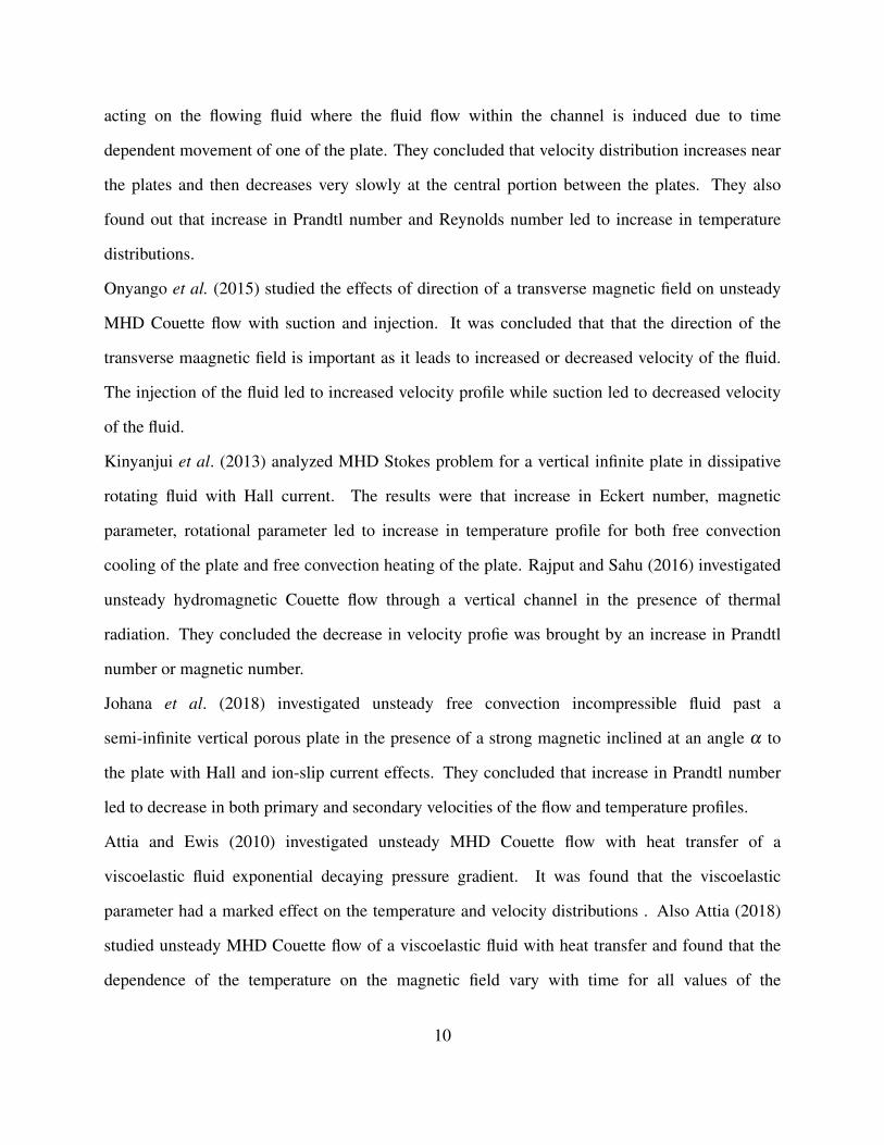
From the Figure 4.1, it is noted that when Reynolds number is raised then the primary velocity

profile rises. Since Reynolds number represents the ratio of inertial forces to viscosity forces, then

an increase in Reynolds number is due to an increase in inertia forces and a decrease in viscous

forces. The force that opposes the motion of the fluid is viscous force, therefore if Reynolds

number(Re) is small, it means that the viscous forces are more dominant than the inertial forces

and thus causes more drag in the fluid thereby a reduction in the flow velocity.

4.2.2 A graph showing the effects of varying Magnetic number on primary

velocity

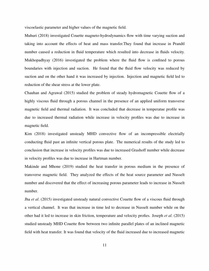
From Figure 4.2, it is noted that when a magnetic parameter increases, then there is a corresponding

decrease in primary velocity of the flowing fluid. This is due to the presence of Lorentz force that

31

Figure 4.1: Velocity profiles for varied values of the Reynolds number, Re.

is caused by magnetic field acting normally to the fluid. The Lorentz force opposes the motion of

the flow since it acts on opposite direction.

4.2.3 A graph showing the effects of varying permeability parameter on

primary velocity

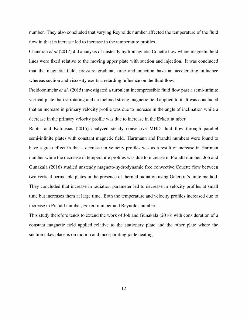
From Figure 4.3, it is observed that increase in primary velocity profile is due to a decrease in

permeability parameter (X). Increased porosity of the medium increases the permeability

parameter thereby reducing the fluid flow acceleration. Increased permeability reduces the

acceleration of the fluid flowing since the pores that would have allowed the fluid to flow with less

restriction closes and as a result the primary velocity decreases.

32

Figure 4.2: Velocity profiles for varied values of the Magnetic number, M.

4.2.4 A graph showing the effects of varying Reynolds number on secondary

velocity, Re

From the Figure 4.4, it is noted that secondary velocity increases due to increase in Reynolds

number. When the viscous forces reduces then there will be a reduction in the opposition of the

motion of the fluid therefore the fluid velocity increases and when the inertial forces reduces then

Reynolds number will decrease which means that there will be dominant viscous forces.

33

Figure 4.3: Velocity profiles for varied values of the X number.

4.2.5 A graph showing the effects of varying permeability parameter on

secondary velocity

From Figure 4.5, it is noted that decrease in secondary velocity profile is due to increased

permeability parameter (X). Increased porosity of the medium raises the permeability parameter

which causes a reduction in acceleration of the flow. Hence reduction in secondary velocity

profile.

34

Figure 4.4: Velocity profiles for varied values of the Reynolds number, Re.

4.2.6 A graph showing the effects of varying Prandtl number on

Temperature profile

From Figure 4.6, it is noted that a rise in the temperature profiles is due to increase in Prandtl

number. Prandtl number is defined as the ratio of viscous diffusion rate to thermal diffusion.

Increase in Prandtl number means low thermal diffusivity of the fluid which leads to increased

internal temperature of the fluid.

35

Figure 4.5: Velocity profiles for varied values of the x number.

4.2.7 A graph showing the effects of varying Reynolds number on

Temperature profile

From the graph 4.7, it is noted that temperature profiles increases if there is an increase in Reynolds

number. A decrease in viscous forces means that there is reduced inertial forces thereby leading to

increased motion of particles of the fluid. Heat is generated due to collision of the particles which

are moving at high velocity thereby increasing the fluids temperature.

36

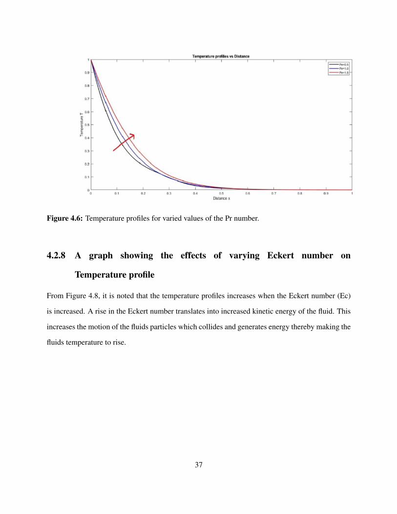
Figure 4.6: Temperature profiles for varied values of the Pr number.

4.2.8 A graph showing the effects of varying Eckert number on

Temperature profile

From Figure 4.8, it is noted that the temperature profiles increases when the Eckert number (Ec)

is increased. A rise in the Eckert number translates into increased kinetic energy of the fluid. This

increases the motion of the fluids particles which collides and generates energy thereby making the

fluids temperature to rise.

37

Figure 4.7: Temperature profiles for varied values of the Re number.

4.2.9 A graph showing the effects of varying Joule heating parameter (R)

Temperature profile

From Figure 4.9, it is noted that increase in joule heating parameter (R) leads to an increased in

temperature. As the current is induced and starts flowing in the fluid, heat is generated due to the

electrical resistance to the flow of charges thereby increasing the temperature.

38

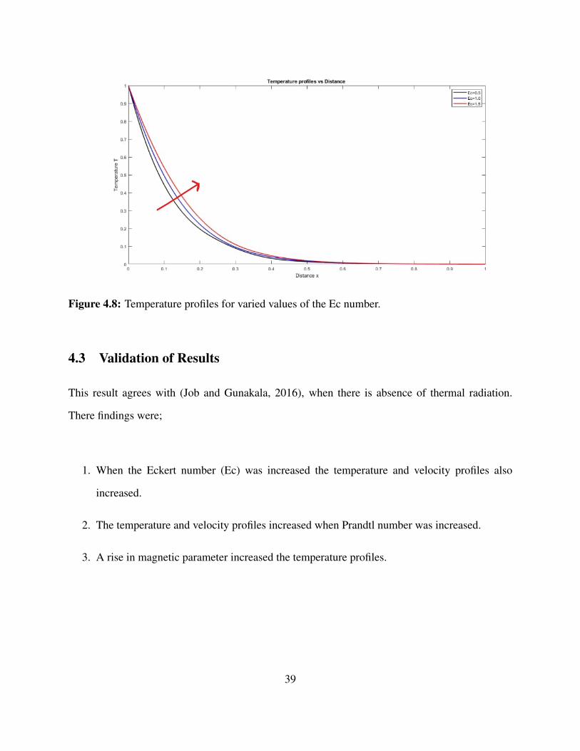
Figure 4.8: Temperature profiles for varied values of the Ec number.

4.3 Validation of Results

This result agrees with (Job and Gunakala, 2016), when there is absence of thermal radiation.

There findings were;

1. When the Eckert number (Ec) was increased the temperature and velocity profiles also

increased.

2. The temperature and velocity profiles increased when Prandtl number was increased.

3. A rise in magnetic parameter increased the temperature profiles.

39

Figure 4.9: Temperature profiles for varied values of the R number.

40

CHAPTER FIVE

CONCLUSION AND RECOMMENDATIONS

5.1 Introduction

This chapter presents a summary of what has been done to attain the objectives and also

recommendations for future research has been presented.

5.2 Conclusions

The results of this study leads to conclusion that;

1. Increase in Reynolds number has an accelerating influence on the primary and secondary

velocity of the flow.

2. Increase in suction and injection parameters leads to decrease in primary flow.

3. Temperature of the flow was affected by Joule Heating parameter (R), Eckert number (Ec)

and Prandtl number (Pr) where by their increase led to increase in temperature of the fluid.

4. Magnetic number and permeability parameter exerts a retarding influence on the fluid

primary and secondary velocity when they are increased.

41

5.3 Recommendations

The study of hydromagnetic Couette flow between two vertical semi-infinite permeable plates with

uniform suction and injection still needs further research. Therefore, my recommendations are;

1. Unsteady hydromagnetic turbulent flow through two vertical infinite plates.

2. Steady hydromagnetic three dimensional Couette flow between vertical finite permiable

plates with variable magnetic field at an angle.

3. Unsteady MHD compressible flow past pearmeable vertical plates with chemical reaction.

42

REFERENCES

Ahmed, F. H. A. (2015). Effect of Silver Nitrate Concentrations on pH of Water. Doctoral

dissertation, Sudan University Of Science & Technology Repository.

Anderson, J. D. (2007). Introduction: Downwash and induced drag. Fundamentals of

Aerodynamics, Tata McGraw-Hill Education, 395–400.

Attia, H. A. (2018). Unsteady MHD Couette flow of a viscoelastic fluid with heat transfer.

Kragujevac J. Sci, 32, 5–15.

Attia, H. A. and Ewis, K. M. (2010). Unsteady MHD Couette flow with heat transfer of a

viscoelastic fluid under exponential decaying pressure gradient. Int. J. Appl. Math. Mech, 13(4),

359–364.

Bodosa, G. and Borkakati, A. (2017). MHD flow with heat transfer between two horizontal plates

in the presence of a uniform transverse magnetic field. Theoretical and Applied Mechanics,

30(1), 1–9.

Boniface, K., Jackson, K., and Thomas, O. (2014). Investigation of hydro magnetic steady flow

between two infinite parallel vertical porous plates. American Journal of Applied Mathematics,

2(5), 170–178.

Chandran, P., Sacheti, N. C., and Singh, A. (2017). Effect of rotation on unsteady hydromagnetic

Couette flow. Astrophysics and Space Science, 202(1), 1–10.

Chauhan, D. S. and Agrawal, R. (2015). Effects of hall current on MHD flow in a rotating channel.

Chemical Engineering Communications, 197(6), 830–845.

De Andrade, V. and Pereira, J. (2015). Gravitational lorentz force and the description of the

gravitational interaction. Physical Review D, 56(8), 4689.

43

Freidoonimehr, N., Rashidi, M. M., and Mahmud, S. (2015). Unsteady MHD free convective

flow past a stretching vertical porous surface. International Journal of Thermal Sciences, 87,

136–145.

Jha, B. K., Samaila, A. K., and Ajibade, A. O. (2015). Unsteady natural convection Couette flow of

a reactive viscous fluid in a vertical channel. Computational Mathematics and Modeling, 24(3),

432–442.

Job, V. M. and Gunakala, S. R. (2016). Unsteady mhd free convection Couette flow between two

vertical permeable plates in the presence of thermal radiation using galerkin’s finite element

method. International Journal of Mechanical Engineering, 2(5), 99–110.

Johana, S. K., Okelo, J., Gatheri, F. K., Ngesa, J. O. (2018). MHD flow past a porous infinite

vertical plate. vertical porous plate with joule heating. Scientific Research Journal, 4(5), 825–

833

Joseph, K., Daniel, S., and Joseph, G. (2015). Unsteady MHD flow through two infinite parallel

porous plates where there is an inclined magnetic field with heat transfer. International Journal

of Mathematics and Statistics Invention, 2(3), 103–110.

Muhuri, P. (2018). Flow formation in Couette motion in magnetohydrodynamics with suction. J.

Phys. Soci. J, 18(11), 1671–1675.

Kim, Y. J. (2018). MHD flow past a semi-infinite porous vertical moving plate with variable

suction. International journal of engineering science, 38(8), 833–845.

Kinyanjui, M., Chaturvedi, N., and Uppal, S. (2013). Stokes problem for an infinite vertical plate

with hall current. Energy conversion and Management, 39(n5-6), 541–548.

Makinde, O. and Mhone, P. (2019). Heat transfer to mhd oscillatory flow in a channel filled with

porous medium. Romanian Journal of physics, 50(n9-10), 931.

44

Onyango, E. R and Kinyanjui, M. N and Kimathi, M (2015). Effects of Direction of Transverse

Magnetic Field on MHD Couette Flow. International Journal of Education and Research, 4(2),

150

Onyango, E. R and Kinyanjui, M. N and Uppal, S. M (2017). Unsteady hydromagnetic Couette

flow with the magnetic field being fixed on the side of the moving upper plate. American Journal

of Applied Mathematics, 3(5), 206

Mukhopadhyay, S. (2016). The analysis of a boundary layer flow over a porous non-linearly

stretching sheet with partial slip at the boundary. Alexandria Engineering Journal, 52(4), 563–

569.

Rajput, U. and Sahu, P. (2016). Natural convection in unsteady hydromagnetic Couette flow

through a channel in the presence of thermal radiation. Int. J. Appl. Math. Mech, 8(3), 35–56.

Raptis, A. and Kafousias, N. (2015). Magnetohydrodynamic free convective flow and mass transfer

through a medium bounded by an infinite vertical permeable plate with constant heat flux.

Canadian Journal of Physics, 60(12), 1725–1729.

Seth, G., Ansari, M. S., and Nandkeolyar, R. (2017). Effects of rotation and magnetic field on

unsteady Couette flow in a porous channel. Journal of Applied Fluid Mechanics, 4(2), 95–103

Steenbrink, A. and Van der Giessen, E. (2016). On cavitation, post-cavitation and yield in

amorphous polymer–rubber blends. Journal of the Mechanics and Physics of Solids, 47(4),

843–876.

45

APPENDICES

Appendix I: Published Article

Owuor, O. C., Kinyanjui, M. N., & Kiogora, P. R. (2020). Hydromagnetic Couette Flow between

Two Vertical Semi-Infinite Permeable Plates. International Journal of Advances in Applied

Mathematics and Mechanics, 7, 1-13.

46

Appendix II: MATLAB Codes

MAIN FUNCTION

function[u,w,T,x]=Adriel(M,X,Ec,Pr,Re,Gr,R,wo) clc

str=1; n=2;

xmax=1;zmax=1;tmax=1;xsteps=32;zsteps=64; tsteps=1000;

x = linspace(0,1,xsteps-23); y = linspace(0,1,xsteps-22);

p = linspace(0,1,xsteps-1); u= zeros(xsteps,tsteps);

w= zeros(xsteps,tsteps); T= zeros(xsteps,tsteps);

dx=0.005; dz=0.005; dt=0.001; rem boundary conditions

initial

for i=1:xsteps for j=1:zsteps for k=1:tsteps u(i,j,1)=0; w(i,j,1)=0; T(i,j,1)=1; end end end for

i=2:xsteps for j=1:zsteps for k=2:tsteps

u(i,1,k)=1; w(i,1,k)=0 ; T(i,1,k)=0; end end end

for i=2:xsteps for j=2:zsteps for k=2:tsteps

u(i,zsteps,k) = i∗ str ∗ (dx)n; w(i,zsteps,k)=0.0; T(i,zsteps,k)=1;

end end end

for i=1:xsteps for j=2:zsteps for k=2:tsteps

u(1,j,k)=1; w(1,j,k)=0; T(1,j,k)=1; end end end

Solving for velocities and temperature

for i=2:xsteps-1 for j=2:zsteps-1 for k=2:tsteps-1 u(i, j,k+1) = (u(i, j,k)/dt− (wo/(4∗dz))∗

(u(i, j+1,k+1)−u(i, j−1,k+1)+u(i, j+1,k)−u(i, j−1,k))+Gr∗T (i, j,k+1)+(1/(2∗Re∗

dx2)) ∗ (u(i+ 1, j,k+ 1)+ u(i− 1, j,k+ 1)+ u(i+ 1, j,k)+ u(i− 1, j,k)− 2 ∗ u(i, j,k))+ (1/(2 ∗

Re∗dz2))∗ (u(i, j+1,k+1)+

u(i, j−1,k+1)+u(i, j+1,k)+u(i, j−1,k)−2∗u(i, j,k)))/(1/dt +(1/(4∗dx))∗ (u(i+1, j,k+

47

1)−u(i−1, j,k+1)+u(i+1, j,k)−u(i−1, j,k))+1/(Re∗dx2)+1/(Re∗dz2)+X +M);

w(i, j,k+1) = (u(i, j,k)/dt− (u(i, j,k+1)/(4∗dx))∗ (w(i+1, j,k+1)−w(i−1, j,k+1)+

w(i+ 1, j,k)−w(i− 1, j,k))−wo ∗ (1/(4 ∗ dz)) ∗ (w(i, j+ 1,k+ 1)−w(i, j− 1,k+ 1)+w(i, j+

1,k)−w(i, j− 1,k))+ (1/(2 ∗Re ∗ dx2)) ∗ (w(i+ 1, j,k+ 1)+w(i− 1, j,k+ 1)+w(i+ 1, j,k)+

w(i− 1, j,k)− 2 ∗w(i, j,k))+ (1/(2 ∗Re ∗ dz2)) ∗ (w(i, j+ 1,k+ 1)+w(i, j− 1,k+ 1)+w(i, j+

1,k)+w(i, j−1,k)−2∗w(i, j,k)))/(1/dt +1/(Re∗dx2)+1/(Re∗dz2)+X); T (i, j,k+1) =

(T (i, j,k)/dt−u(i, j,k+1)∗ (1/(4∗dx))∗ (T (i+1, j,k+1)−T (i−1, j,k+1)+T (i+1, j,k)−

T (i−1, j,k))−w(i, j,k+1)∗ (1/(4∗dz))∗ (T (i, j+1,k+1)−T (i, j−1,k+1)+T (i, j+1,k)−

T (i, j−1,k))+(1/(2∗Re∗Pr∗dx2))∗(T (i+1, j,k+1)+T (i−1, j,k+1)+T (i+1, j,k)+T (i−

1, j,k)− 2 ∗ T (i, j,k)) + (1/(2 ∗Re ∗Pr ∗ dz2)) ∗ (T (i, j + 1,k + 1) + T (i, j− 1,k + 1) + T (i, j +

1,k)+ T (i, j− 1,k)− 2 ∗ T (i, j,k))+Re ∗R ∗ (u(i, j,k+ 1))2 +((Ec)/(16 ∗Re ∗ dz2)) ∗ (w(i, j +

1,k+ 1)+w(i, j+ 1,k)−w(i, j− 1,k+ 1)−w(i, j− 1,k))2 +((Ec)/(Re)) ∗ ((u(i+ 1, j,k+ 1)+

u(i+1, j,k)−u(i−1, j,k+1)−u(i−1, j,k))/(4∗dx))2)/(1/dt+1/(Re∗Pr∗dx2)+1/(Re∗Pr∗

dz2));

end end end

PRIMARY PROFILES

figure(1) clc; clear; [u,w,T,x] = Adriel(M,X ,Ec,Pr,Re,Gr,R,wo) Changing Re

[u,w,T,x] = Adriel(10,20,0.5,0.71,70,0.5,0.5,0.05); x1= 0:0.01:1;

y1=spline(x,u(1:9,10,10),x1); plot(x1 ,y1,’ k’ ,’Linewidth’,1.5,’LineSmoothing’,’on’);

title(’Primary velocity profiles vs Distance’); xlabel(’Distance x’); ylabel(’Velocity u’);

SECONDARY PROFILES

figure(2) hold on clc; clear; [u,w,T,x] = Adriel(M,X ,Ec,Pr,Re,Gr,R,wo) Changing Re

[u,w,T,x] = Adriel(10,20,0.5,0.71,70,0.5,0.5,0.05); x1= 0:0.01:1;

48

y1=spline(x,w(1:9,10,10),x1); plot(x1 ,y1,’ k’ ,’Linewidth’,1.5,’LineSmoothing’,’on’); hold on

[u,w,T,x] = Adriel(10,20,0.5,0.71,80,0.5,0.5,0.05); x2= 0:0.01:1;

y2=spline(x,w(1:9,10,10),x2); plot(x2 ,y2,’ g’ ,’Linewidth’,1.5,’LineSmoothing’,’on’); hold on

[u,w,T,x] = Adriel(10,20,0.5,0.71,90,0.5,0.5,0.05); x3= 0:0.01:1;

y3=spline(x,w(1:9,10,10),x3); plot(x3 ,y3,’ b’ ,’Linewidth’,1.5,’LineSmoothing’,’on’); hold on

[u,w,T,x] = Adriel(10,20,0.5,0.71,100,0.5,0.5,0.05); x5= 0:0.01:1;

y5=spline(x,w(1:9,10,10),x5); plot(x5 ,y5,’ r’ ,’Linewidth’,1.5,’LineSmoothing’,’on’);

title(’Secondary velocity profiles vs Distance’); xlabel(’Distance x’); ylabel(’Velocity w’);

legend(’Re=70’,’Re=80’,’Re=90’,’Re=100’) hold off

TEMPERATURE PROFILES

figure(3) [u,w,T,x] = Adriel(10,20,0.5,0.71,60,0.5,0.5,0.05); x1= 0:0.01:1;

y1=spline(x,T(1:9,10,10),x1); plot(x1 ,y1,’ r’ ,’Linewidth’,1.5,’LineSmoothing’,’on’);

title(’Temperature profiles vs Distance ’); xlabel(’Distance x’); ylabel(’Temperature T’);

49