topic 10 gis modeling procedures - innovative gis

Topic 10 – GIS Modeling Procedures ______________________________________________________________________________________

______________________________________________________________________________________ Analyzing Geo-Spatial Resource Data 10-1

Topic 10

GIS Modeling Procedures

10.1 Constitution of a GIS Model A topic that consistently captures the imagination of GIS users going beyond mapping is “what are the types and characteristics of GIS models?” The following outline is the current state of "sourdough" thinking collected over the years from numerous articles, presentations and informal discussion with academicians, software developers and general GIS users. What do you think?

Do you know of any model types or characteristics missing from the outline? Are any in the outline misrepresented?

The following are other terms often used to describe models: physical, atomistic, holistic,

constrained, fragmented, dispersed, data, analytical, diffusion, scale, optimizing, simulation, analytical, process, synthetic, systems, flow, statistical, mathematical, hierarchical, binary... Can you explain what is meant by these terms? Are any relevant? Where might they fit into the outline?

Do you see any utility in developing a comprehensive classification scheme for GIS

modeling? ...or is this just another esoteric and academic (gee, that might be redundant) exercise? Who would benefit from such an outline?

_______________________ TYPES AND CHARACTERISTICS OF GIS MODELS 1.0 MODELING: a model is a representation of reality in either Material form (physical representation) or Symbolic form (abstract representation); GIS modeling involves symbolic representation of Locational properties (WHERE), as well as Thematic (WHAT) and Temporal (WHEN) attributes describing characteristics and conditions of space and time. 2.0 GENERAL TYPES OF MODELS: Structural and Relational

2.1 Structural: focus on the composition and construction of things; Object and Action are two types of structural models.

2.1.1 Object Model — Static Entity-based which forms a visual representation of an item; e.g., an architect's blueprint of a building. Characteristics include scaled, 2 or 3-dimensional, symbolic representation. 2.1.2 Action Model — Dynamic Movement-based which tracks the space/time relationships of items; e.g., a model train along it's track. Characteristics include time-slices, change detection, transition statistics, animation.

2.2 Relational: focus on the interdependence and relationships among factors; Functional and

Conceptual are two types of relational models.



2.2.1 Functional Model — Input/Output-based which tracks relationships among variables, such as storm runoff prediction. Characteristics include cause/effect linkages, “hard” science, and sensitivity analysis. 2.2.2 Conceptual Model — Perception-based which incorporates both fact interpretation and value weights, such as suitability for outdoor recreation. Characteristics include heuristics (expert rules), “soft” science, scenarios.

3.0 TYPES OF GIS MODELS: Cartographic and Spatial

3.1 Cartographic Model — automation of manual techniques which traditionally use drafting aids and transparent overlays, such as a map identifying locations of productive soils and gentle slopes using binary logic expressed as a geo-query.

3.2 Spatial Model — expression of mathematical relationships among mapped variables, such as a map of crop yield throughout a field based on relative amounts of phosphorous, potassium, nitrogen and ph levels using multi-value logic expressed as variables, parameters and relationships.

4.0 GIS MODEL CHARACTERISTICS: Scale, Extent, Purpose, Approach, Technique, Association and Aggregation

4.1 Scale: Micro and Macro

4.1.1 Micro — contains high-resolution of space, time and/or variable considerations governing system response, such as a 1:1,000 map of a farm with the crop specified for each individual field that is revised each year. 4.1.2 Macro — contains low-resolution of space, time and/or variable considerations governing system response, such as a 1:1,000,000 map of land use with single category for agriculture that is revised every ten years.

4.2 Extent: Complete and Partial

4.2.1 Complete — includes entire set of space, time and/or variable considerations governing system response, such as a map of an entire watershed or river basin. 4.2.2 Partial — includes subsets of space, time and/or variable considerations governing system response, such as a standard topographic sheet with its "artificial edge" capturing limited portions of several adjoining watersheds.

4.3 Purpose: Descriptive and Prescriptive

4.3.1 Descriptive — characterization of the direct interactions of system components to gain insight into system processes (understand), such as a wildlife population dynamics map generated by simulation of birth and death processes. 4.3.2 Prescriptive — characterization of correlated factors that are related to system response used in determining appropriate management action (decide), such as a a sales prediction map based on census block-level demographic in formation.

4.4 Approach: Empirical and Theoretical



4.4.1 Empirical — based on reduction (analysis) of field collected measurements, such as a map of soil loss for each watershed in a region generated by spatially evaluating the Universal Soil Loss Equation.

4.4.2 Theoretical — based on the linkage (synthesis) of proven or postulated relationships among variables, such a map of spotted owl habitat based on accepted theories on owl preferences.

4.5 Technique: Deterministic and Stochastic

4.5.1 Deterministic — direct evaluation of a defined relationship (results in a single repeatable solution), such as a wildlife population map based on one model execution using a single "best" estimate to characterize each variable. 4.5.2 Stochastic — simulation of a probabilistic relationship (results in a range of likely solutions), such as a wildlife population map based on the average of a series of model executions using probability functions to characterize each variable.

4.6 Association: Lumped and Linked

4.6.1 Lumped — the state/condition of each individual map location is based on the independent values of other variables at that location (point-by-point), such as land cover map based on the relative amounts of reflected light from satellite imagery.

4.6.2 Linked — the state/condition of an individual map location is dependent on the conditions of surrounding map locations (vicinity, neighborhood or region), such as an overland flow model considering terrain configuration and intervening soil conditions.

4.7 Aggregation: Cohort and Disaggregated

4.7.1 Cohort — executed for groups of objects having similar characteristics, such as a timber growth map for each management parcel based on a look-up table of growth for each specific set of landscape conditions (usually vector-based polygons).

4.7.2 Disaggregated — executed for each individual object, such as a map of predicted biomass based on spatially evaluating a regression equation in which each input map identifies an independent variable, each location a case, and each value a measurement (usually raster-based grid cells).

4.8 Temporal: Static and Dynamic

4.8.1 Static — treats time as constant and model variables do not vary over time, such as a map of current timber value based on forest inventory and relative access to existing roads.

4.8.2 Dynamic — treats time as variable and model variables change as a function of time, such as a map of the spread of a pollution plume from a point source driven by wind direction/strength and relative humidity.

10.2 A Classification Guide for GIS Models As you might have gleamed from dozing off face down on the previous outline of GIS model types and characteristics, there are several dimensions for classifying models. Hopefully you wrestled with the brief



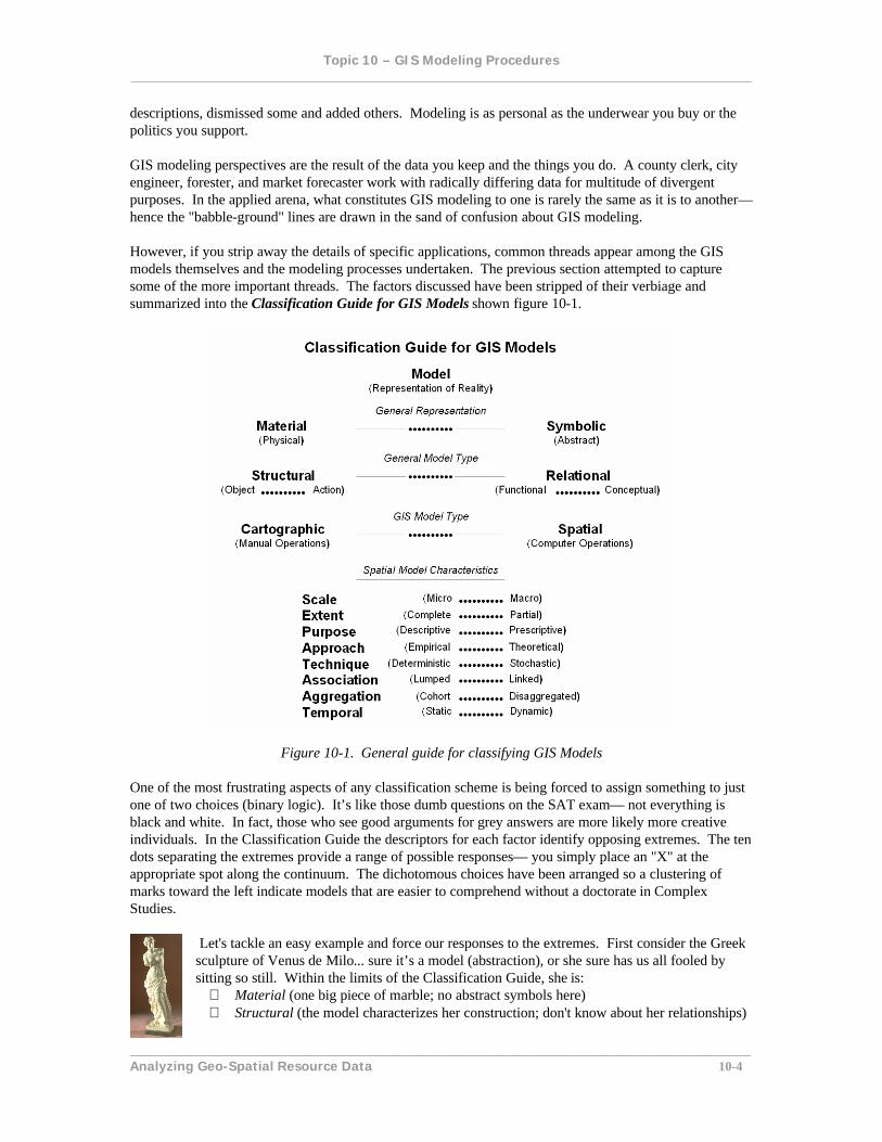
descriptions, dismissed some and added others. Modeling is as personal as the underwear you buy or the politics you support. GIS modeling perspectives are the result of the data you keep and the things you do. A county clerk, city engineer, forester, and market forecaster work with radically differing data for multitude of divergent purposes. In the applied arena, what constitutes GIS modeling to one is rarely the same as it is to another— hence the "babble-ground" lines are drawn in the sand of confusion about GIS modeling. However, if you strip away the details of specific applications, common threads appear among the GIS models themselves and the modeling processes undertaken. The previous section attempted to capture some of the more important threads. The factors discussed have been stripped of their verbiage and summarized into the Classification Guide for GIS Models shown figure 10-1.

Figure 10-1. General guide for classifying GIS Models One of the most frustrating aspects of any classification scheme is being forced to assign something to just one of two choices (binary logic). It’s like those dumb questions on the SAT exam— not everything is black and white. In fact, those who see good arguments for grey answers are more likely more creative individuals. In the Classification Guide the descriptors for each factor identify opposing extremes. The ten dots separating the extremes provide a range of possible responses— you simply place an "X" at the appropriate spot along the continuum. The dichotomous choices have been arranged so a clustering of marks toward the left indicate models that are easier to comprehend without a doctorate in Complex Studies.

Let's tackle an easy example and force our responses to the extremes. First consider the Greek sculpture of Venus de Milo... sure it’s a model (abstraction), or she sure has us all fooled by sitting so still. Within the limits of the Classification Guide, she is:

Material (one big piece of marble; no abstract symbols here) Structural (the model characterizes her construction; don't know about her relationships)



Object (visual rendering of just her; no movable parts) Now she's not a GIS Model, but if she were she would be: Cartographic (manual techniques; no wimpy mathematics) Micro (about a 1:1 scale; unless she's a scaled-down version of Goliath's mom) Partial (missing arms and legs; or maybe she had a run-in with a chainsaw) Descriptive (wow, and how; doesn't tell you what to do ...she's just a rock) Empirical (direct measurement; or the sculptor had an active imagination) Deterministic (direct single solution; hips and shoulders have no chance of being attached elsewhere) Linked (the hip bone is connected to the thigh bone...; can't talk about her chin without noticing her

eyes) Disaggregated (one-of-a-kind; though millions strive for a favorable comparison) Static (hasn't changed for centuries; the whole effect is dynamite, but not dynamic)

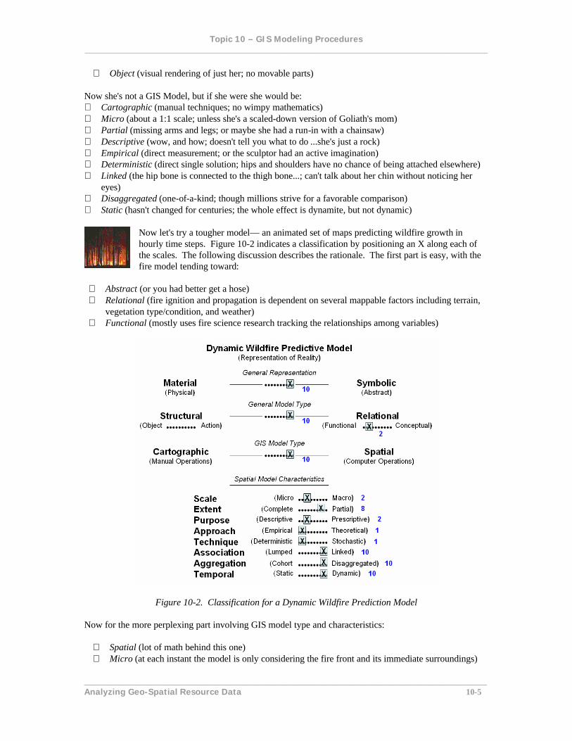
Now let's try a tougher model— an animated set of maps predicting wildfire growth in hourly time steps. Figure 10-2 indicates a classification by positioning an X along each of the scales. The following discussion describes the rationale. The first part is easy, with the fire model tending toward:

Abstract (or you had better get a hose) Relational (fire ignition and propagation is dependent on several mappable factors including terrain,

vegetation type/condition, and weather) Functional (mostly uses fire science research tracking the relationships among variables)

Figure 10-2. Classification for a Dynamic Wildfire Prediction Model Now for the more perplexing part involving GIS model type and characteristics:

Spatial (lot of math behind this one) Micro (at each instant the model is only considering the fire front and its immediate surroundings)



Partial (until the fire is extinguished) Descriptive (unabated fire propagation without fire management actions) Empirical (based on field calibrated equations) Deterministic (based on a defined set of input parameters) Linked (adjacent parcels are the next to burn) Disaggregated (independently considers each burning location and its propagation options) Dynamic (both diurnal and on-going fire behavior conditions change model variables)

Whew! …that’s a lot of detail for map normally taken at face value. Now try your hand at "classifying" the following representations of reality and/or your own favorite models:

Mount Rushmore's faces of the presidents A landscape architect's raised-relief cardboard model of a National Park An elk habitat map A set of seasonal maps of elk habitat An elk population dynamics model responding to landscape conditions and predator/prey

interactions A GIS implementation of the Universal Soil Loss Equation for a watershed A GIS implementation of the Horton Overland Flow Equations evaluating surface water runoff for a

set of watersheds A crop yield prediction map Maps of wildfire risk generated each morning

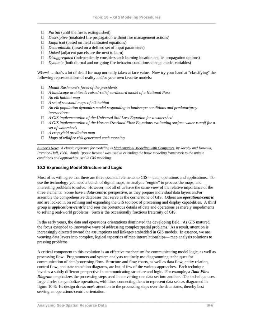
__________________________________ Author's Note: A classic reference for modeling is Mathematical Modeling with Computers, by Jacoby and Kowalik, Prentice-Hall, 1980. Ample "poetic license" was used in extending the basic modeling framework to the unique conditions and approaches used in GIS modeling. 10.3 Expressing Model Structure and Logic Most of us will agree that there are three essential elements to GIS— data, operations and applications. To use the technology you need a bunch of digital maps, an analytic "engine" to process the maps, and interesting problems to solve. However, not all of us have the same view of the relative importance of the three elements. Some have a data-centric perspective, as they prepare individual data layers and/or assemble the comprehensive databases that serve as the cornerstone of GIS. Others are operations-centric and are locked in on refining and expanding the GIS toolbox of processing and display capabilities. A third group is applications-centric and sees the portentous details of data and operations as merely impediments to solving real-world problems. Such is the occasionally fractious fraternity of GIS. In the early years, the data and operations orientations dominated the developing field. As GIS matured, the focus extended to innovative ways of addressing complex spatial problems. As a result, attention is increasingly directed toward the assumptions and linkages embedded in GIS models. In essence, we are weaving data layers into complex, logical tapestries of map interrelationships— map analysis solutions to pressing problems. A critical component to this evolution is an effective mechanism for communicating model logic, as well as processing flow. Programmers and system analysts routinely use diagramming techniques for communication of data/processing flow. Structure and flow charts, as well as data flow, entity relation, control flow, and state transition diagrams, are but of few of the various approaches. Each technique invokes a subtly different perspective in communicating structure and logic. For example, a Data Flow Diagram emphasizes the processing steps used in converting one data set into another. The technique uses large circles to symbolize operations, with lines connecting them to represent data sets as diagramed in figure 10-3. Its design draws one's attention to the processing steps over the data states, thereby best serving an operations-centric orientation.



Figure 10-3. Data Flow Diagram.

Processing-oriented diagrams work well for non-spatial information processing. They relate data about entities through indexed files. In these instances, the specifications in a database query are paramount. Instances of geo-query, such as "where are all the locations that have slopes over 13% AND unstable soils AND are devoid of vegetation," use standard database management systems technology. Standard diagramming techniques, in such instances, are most appropriate. However, spatial analysis techniques go beyond the repackaging of existing data. For example, if you want establish variable-width buffers around salmon spawning streams it's a different story. You need to simultaneously consider intervening slopes, ground cover, and soil stability as you "measure" distance. If you want to establish a map of visual exposure density to roads, you need to consider maps of the road network, relative elevations at a minimum. These, and the myriad of other spatial analysis procedures, have strong data dependency. They are not just setting a few parameters for traditional, non-spatial processing techniques. Spatial analysis is an entirely new kettle of fish. It is dependent upon the unique geographic patterns of the data sets involved— definitely data-centric conditions.

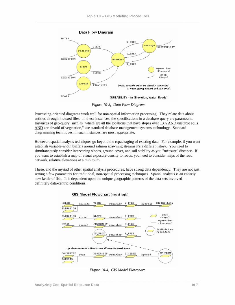
Figure 10-4. GIS Model Flowchart.



A GIS Modeling Flowchart takes such a perspective. The top portion figure 10-4 uses a flowchart to track the same data/processing steps as shown in the Data Flow Diagram. However, maps (i.e., data sets) are depicted as boxes and operations (i.e., processing steps) are depicted as lines. This focus is obviously data-centric as it draws your attention to the mapped variables, but also it is arguably an applications-centric one as well. Most users of GIS have prior experience with manual map analysis techniques. They have struggled with rulers, dot grids, and transparent overlays to laboriously draft new maps that better address a question at hand. For example, you may have circled areas where the elevation contour lines are close together to create a map of steep slopes. In doing so, attention is focused on the elevation data and the resultant circles inscribed on the transparent overlay— the input and output maps. The bottom portion of the figure shows a logic modification incorporating a preference to be “near or within diverse forested areas.” A neighborhood operation (scan) assigns the number of different vegetation types (COVERTYPE) within the vicinity of each forested location (FORESTS). Areas of high diversity are isolated (renumber), and a proximity map from these areas (DF_PROX) is generated for the entire project area. Since several models might share this command set, it is stored as a generalized procedure and is simply attached using the SubModel or Procedure flowcharting "widget."

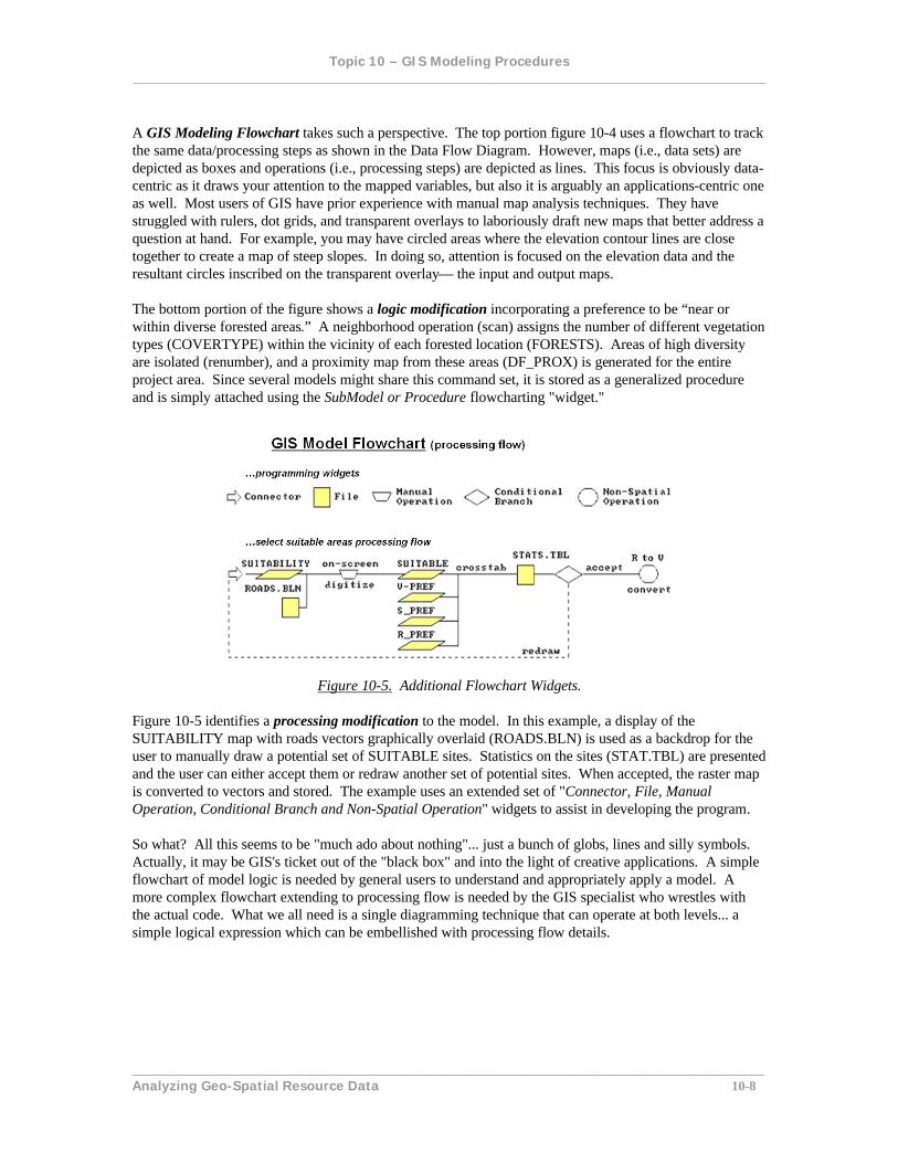
Figure 10-5. Additional Flowchart Widgets.

Figure 10-5 identifies a processing modification to the model. In this example, a display of the SUITABILITY map with roads vectors graphically overlaid (ROADS.BLN) is used as a backdrop for the user to manually draw a potential set of SUITABLE sites. Statistics on the sites (STAT.TBL) are presented and the user can either accept them or redraw another set of potential sites. When accepted, the raster map is converted to vectors and stored. The example uses an extended set of "Connector, File, Manual Operation, Conditional Branch and Non-Spatial Operation" widgets to assist in developing the program. So what? All this seems to be "much ado about nothing"... just a bunch of globs, lines and silly symbols. Actually, it may be GIS's ticket out of the "black box" and into the light of creative applications. A simple flowchart of model logic is needed by general users to understand and appropriately apply a model. A more complex flowchart extending to processing flow is needed by the GIS specialist who wrestles with the actual code. What we all need is a single diagramming technique that can operate at both levels... a simple logical expression which can be embellished with processing flow details.



10.4 Recipes for Solving Spatial Problems So what is the difference between a recipe and a model? Both seem to mix a bunch of things together to create something else. Both result in a synergistic amalgamation that is something more than simply the sum of the parts. Both start with basic ingredients and describe the processing steps required to produce the desired result— be it a chocolate cake, or a landslide susceptibility map. In a GIS, the ingredients are the base maps and the processing steps are the spatial handling operations employed. For example, a simple recipe for locating landslide susceptibility involves the ingredients of terrain steepness, soil type and vegetation cover— with areas that are steep, unstable and bare being the most susceptible to landslides. Before computers, the identification of the areas of high susceptibility involved tedious manual map analysis procedures. A transparency was taped over a contour map of elevation and areas where the contour lines were closely spaced (steep) were outlined and filled with a dark color. Similar "transparent overlays" were interpreted for areas of unstable soils and sparse vegetation from base maps of soils and vegetation. When the three transparencies were overlaid on a strong light source, the combination was easily deciphered— clear= not susceptible and dark= susceptible. This basic recipe has been with us for quite some time. Of course the methods have subtly changed with modern drafting aids replacing thin parchment, quill pens and stained glass windows of the 1800's, but the conceptual approach remains the same. In a typical vector GIS, this logical combination is achieved by first generating a topological overlay of the three maps (SLOPE, SOILS, COVERTYPE), then querying the resultant table (TSV_OVL) for susceptible areas. The SQL query might look like

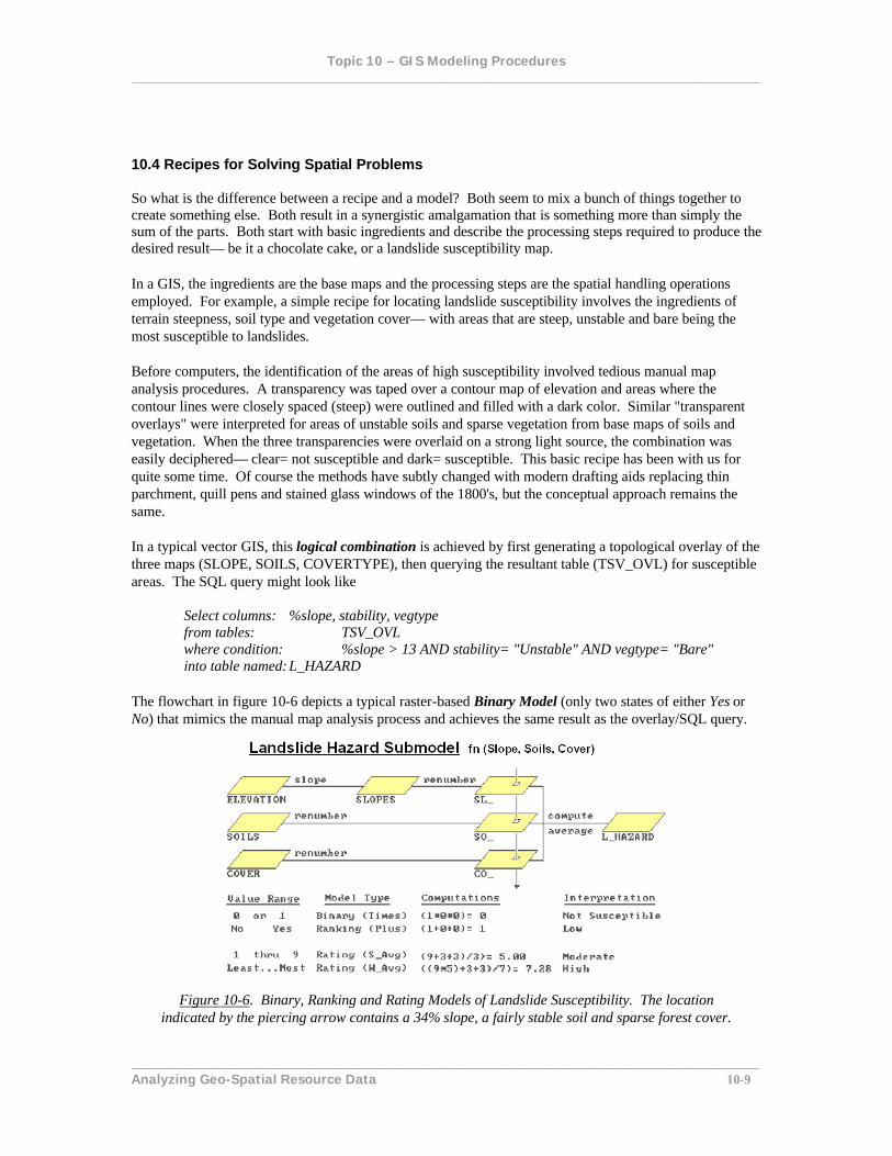
Select columns: %slope, stability, vegtype from tables: TSV_OVL where condition: %slope > 13 AND stability= "Unstable" AND vegtype= "Bare" into table named: L_HAZARD The flowchart in figure 10-6 depicts a typical raster-based Binary Model (only two states of either Yes or No) that mimics the manual map analysis process and achieves the same result as the overlay/SQL query.

Figure 10-6. Binary, Ranking and Rating Models of Landslide Susceptibility. The location

indicated by the piercing arrow contains a 34% slope, a fairly stable soil and sparse forest cover.



A slope map is created by calculating the change in elevation throughout the project area (first derivative of the elevation surface). A binary solution codes as 1's all of the susceptible areas on each of the factor maps (>30% slope; unstable soils; bare vegetative cover); whereas the non-susceptible areas are coded as 0's. The product of the three binary maps (SL_binary, SO_binary, CO_binary) creates a final map of landslide potential— 1= susceptible and 0= not susceptible. Only locations which are susceptible on all three maps retain the "susceptible" classification (1*1*1= 1). In the other instances, multiplying 0 times any number forces the product to 0 (not susceptible). The map-ematical model corresponding to the flowchart in the figure might be expressed in the MapCalc modeling language as— SLOPE ELEVATION FOR SLOPES …create slope map RENUMBER SLOPES FOR SL_binary ASSIGNING 0 TO 0 THRU 12 ASSIGNING 1 TO 13 THRU 1000 …> 13%, steep RENUMBER SOILS FOR SO_binary ASSIGNING 0 TO 0 THRU 2 ASSIGNING 1 TO 3 THRU 4 …soils 3&4, unstable RENUMBER COVERTYPE FOR CO_binary ASSIGNING 0 TO 1 ASSIGNING 0 TO 3 ASSIGNING 1 TO 2 …cover 2, bare COMPUTE SL_binary TIMES SO_binary TIMES CO_binary FOR L_HAZARD …1*1*1=1, hazard In the multiplicative case, the arithmetic combination of the maps yields the original two states— dark or 1= susceptible, and clear or 0= not susceptible. It is analogous to the "AND" condition of the logical combination in the SQL query. However, other combinations can be derived. For example, the visual analysis could be extended by interpreting the various shades of grey on the stack of transparent overlays— clear= not susceptible; light grey= low; medium grey= moderate; and dark grey= high susceptibility. In an analogous map-ematical approach, the computed sum of the three binary maps yields a similar ranking— 0= not susceptible, 1= low, 2= moderate, and 3= high susceptibility (1+1+1= 3). This approach is termed a Ranking Model because it develops an ordinal scale of increasing landslide potential-- a value of two is more susceptible than a value of 1, but not necessarily twice as susceptible. A Rating Model is radically different as it uses a consistent scale with more than two states to characterize the relative landslide potential for various conditions on each of the factor maps. For example, a value of 1 is assigned to the least susceptible steepness condition (e.g., from 0 to 5% slope), while a value of 9 is assigned to the most susceptible condition (e.g., > 30% slope). The intermediate conditions are assigned appropriate values between the landslide susceptibility extremes of 1 and 9. This calibration results in three maps with relative susceptibility ratings (SL_rate, SO_rate, CO_rate) based on the 1 to 9 scale. Computing the simple average of the three rate maps determines an overall landslide potential based on the relative ratings for each factor at each map location. For example, a particular grid cell might be rated a 9 because it is very steep, a 3 because its soil is fairly stable, and a 1 because it is forested. The average landslide susceptibility rating under these conditions is ((9+3+3)/3)= 5.00, indicating a moderate landslide potential. A weighted average of the three maps expresses the relative importance of each of the factors in determining overall susceptibility. For example, steepness might be identified as being "five times" more important than either soils or vegetative cover in estimating landslide potential. For the example grid cell described above, the weighted average computes to (((9*5)+3+3)/7)= 7.28, which is closer to a high overall rating. The weighted average is preferentially influenced by the SL_rate map's high rating, yielding a much higher overall rating than the simple average. All this may be a bit confusing. The four different "recipes" for landslide potential produced strikingly different results for the example grid cell... from not susceptible to high susceptibility. It's like baking



banana bread. Some folks follow the traditional recipe, some add chopped walnuts, and others throw in a few cranberries. About the time diced dates and candied cherries are tossed in, you can't tell the difference between your banana bread and last Christmas's fruitcake. So back to the main point— what's the difference between a recipe and a model? Merely semantics, or marketing jargon? The real difference between a recipe and a model isn't in the ingredients, or the processing steps themselves. It's in the conceptual fabric of the process. 10.5 Extending Model Solutions The previous section described various renderings of a landslide susceptibility model. It related the results obtained for an example location using manual, logical combination, binary, ranking and rating models. The results were strikingly different, ranging from not susceptible to highly susceptible. Two factors in model expression were at play— 1) the type of model and 2) its calibration. However, its model structure, identifying the factors considered and how they interact, remained constant. In the example, the logic was constrained to the joint consideration of terrain steepness, soil type and vegetation cover. One could argue other factors might contribute to landslide potential. What about depth to bedrock? Or previous surface disturbance? Or slope length? Or precipitation frequency and intensity? Or gopher population density? Or about anything else you might dream up. That's it ... the secret to seat-of-the-pants GISing. First you address the "critical" factors, and then extend your attention to other "contributing" factors. In the abstract, this means adding boxes and arrows to the flowchart reflecting the added logic. In practice it means expanding the GIS macro code, and most importantly wrestling with the model's "calibration." For example, it is easy to add a fourth row to the landslide flowchart shown in figure 10-6 by identifying the additional criterion of depth to bed rock and tie it to the other three factors.

It's even fairly easy to add the new lines of code to the GIS macro, such as— RENUMBER DEPTH_BR FOR BR_binary ASSIGNING 0 TO 0 THRU 4 ASSIGNING 1 TO 4 THRU 15 …>4, massive COMPUTE SL_binary TIMES SO_binary TIMES CO_binary TIMES BR-binary FOR L_HAZARD Things get a lot tougher when you have to split hairs about precisely what soil depths increase landslide susceptibility (>4 a good guess?). If you do this in a room filled with a lot of important people, you can call the collective guess-timating the Delphi Method or Expert Systems modeling. If for no other reason, there will be more folks to share the blame if the model doesn't work. The previous discussions have focused on the "hazard" of landslides, but not their "risk." Do we really care about landslides unless there is something of "value" in their way? The term risk implies the threat a hazard imposes on something of value. Common sense suggests that a landslide hazard distant from important features represents a much smaller threat than a similar hazard adjacent to a major road or school. Figure 10-7 shows a Risk Extension to the rating model that considers the proximity to important features as an indicator of risk.



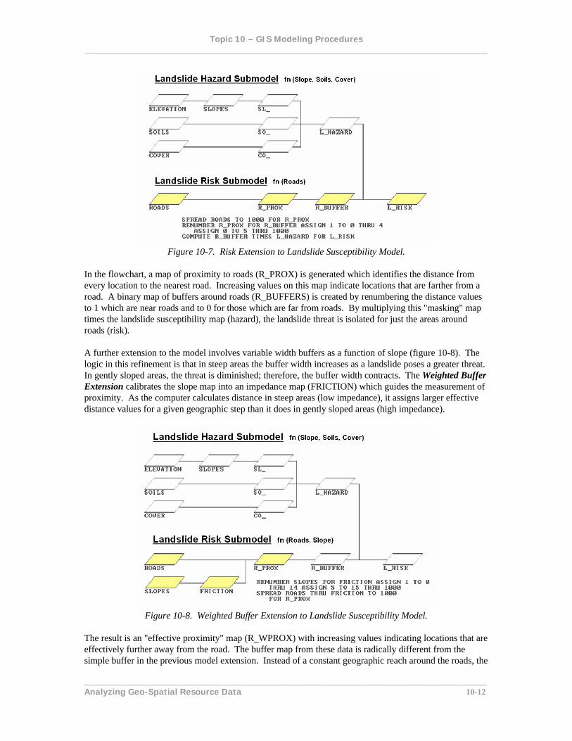
Figure 10-7. Risk Extension to Landslide Susceptibility Model.

In the flowchart, a map of proximity to roads (R_PROX) is generated which identifies the distance from every location to the nearest road. Increasing values on this map indicate locations that are farther from a road. A binary map of buffers around roads (R_BUFFERS) is created by renumbering the distance values to 1 which are near roads and to 0 for those which are far from roads. By multiplying this "masking" map times the landslide susceptibility map (hazard), the landslide threat is isolated for just the areas around roads (risk). A further extension to the model involves variable width buffers as a function of slope (figure 10-8). The logic in this refinement is that in steep areas the buffer width increases as a landslide poses a greater threat. In gently sloped areas, the threat is diminished; therefore, the buffer width contracts. The Weighted Buffer Extension calibrates the slope map into an impedance map (FRICTION) which guides the measurement of proximity. As the computer calculates distance in steep areas (low impedance), it assigns larger effective distance values for a given geographic step than it does in gently sloped areas (high impedance).

Figure 10-8. Weighted Buffer Extension to Landslide Susceptibility Model.

The result is an "effective proximity" map (R_WPROX) with increasing values indicating locations that are effectively further away from the road. The buffer map from these data is radically different from the simple buffer in the previous model extension. Instead of a constant geographic reach around the roads, the



effective buffer varies in width, as a function of slope, throughout the map area. As before, the buffer can be used as a binary mask to isolate the hazards within the variable reach of the roads. This iterative refinement characterizes a typical approach to GIS modeling— from simple to increasingly complex. Most applications first mimic manual map analysis procedures, then are extended to include more advanced spatial analysis tools. For example, a more rigorous map-ematical approach to the previous extension might use a mathematical function to combine directly the effective proximity (R_WPROX) with the relative hazard rating (L_HAZARD) in calculating an index of risk for each location. For your enjoyment, some additional extensions are suggested below. Can you modify the flowchart to reflect the changes in model logic? If you have a copy of the MapCalc software, can you develop the additional code? If you were a malleable undergraduate, you would have to if you wanted to pass the course. Ah, but you’re a professional and need not concern yourself with such details. Just ask the 18 year old GIS hacker down the hall to do your spatial reasoning. HAZARD SUBMODEL MODIFICATIONS

Consideration of other physical factors such as bedrock type, depth to bedrock, faulting, etc. Consideration of disturbance factors, such as construction cuts and fills Consideration of environmental factors, such as recent storm frequency, intensity and duration Consideration of seasonal factors, such as freezing and thawing cycles in early spring Consideration of historical landslide data for the region, such as earthquake frequency RISK SUBMODEL MODIFICATIONS Consideration of additional important features, such as public, commercial and residential structures Extension to differentially weight the uphill and downhill slopes from a feature in calculating the

effective buffer Extension to preferentially weight roads based on traffic volume, emergency routes, etc. Extension to include an economic valuation of the threatened features and potential resource loss 10.6 Infusing Science into GIS Models As the last couple of sections have noted, GIS applications come in a variety of forms. The differences are not as much in the ingredients (maps), nor the processing steps themselves (command macros), as much as it is the conceptual fabric of the process. As noted in the evolution of the landslide susceptibility model, differences can arise through model logic and/or model expression. A simple binary model of susceptibility (only two states of either Yes or No) is radically different from a rating model using a weighted average of relative susceptibility indices. In mathematical terms, the rating model is more "robust" as it provides a continuum of system responses. Also, it provides the foothold to extend the model even farther, as we will soon see. There are two basic types of GIS models— cartographic and spatial. In short, a Cartographic Model focuses on the automation of manual map analysis techniques and reasoning, whereas a Spatial Model focuses on the expression of mathematical relationships. In the landslide example, the logical combination and the binary map algebra solutions are obviously cartographic models. Both could be manually solved using file cabinets and transparent overlays... tedious, but doable. The weighted average rating model, on the other hand, smacks of map-ematics and is a candidate spatial model. But is it? As with most dichotomous classifications there is a grey area of overlap between cartographic and spatial model extremes. If the weights used in rating model averaging are merely "guess-timates," then the application is lacking in all of the rights, privileges and responsibilities of an exalted spatial model. The model may be mathematically expressed, but the logic isn't mathematically derived, or empirically verified. In short, "where's the science?"



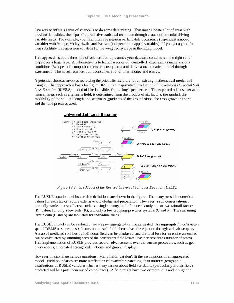
One way to infuse a sense of science is to do some data mining. That means locate a lot of areas with previous landslides, then "push" a predictive statistical technique through a stack of potential driving variable maps. For example, you might run a regression on landslide occurrence (dependent mapped variable) with %slope, %clay, %silt, and %cover (independent mapped variables). If you get a good fit, then substitute the regression equation for the weighted average in the rating model. This approach is at the threshold of science, but it presumes your database contains just the right set of maps over a large area. An alternative is to launch a series of "controlled" experiments under various conditions (%slope, soil composition, cover density, etc.) and derive a mathematical model through experiment. This is real science, but it consumes a lot of time, money and energy. A potential shortcut involves reviewing the scientific literature for an existing mathematical model and using it. That approach is basis for figure 10-9. It's a map-matical evaluation of the Revised Universal Soil Loss Equation (RUSLE)— kind of like landslides from a bug's perspective. The expected soil loss per acre from an area, such as a farmer's field, is determined from the product of six factors: the rainfall, the erodibility of the soil, the length and steepness (gradient) of the ground slope, the crop grown in the soil, and the land practices used.

Figure 18-3. GIS Model of the Revised Universal Soil Loss Equation (USLE).

The RUSLE equation and its variable definitions are shown in the figure. The many possible numerical values for each factor require extensive knowledge and preparation. However, a soil conservationist normally works in a small area, such as a single county, and often needs only one or two rainfall factors (R), values for only a few soils (K), and only a few cropping/practices systems (C and P). The remaining terrain data (L and S) are tabulated for individual fields. The RUSLE model can be evaluated two ways-- aggregated or disaggregated. An aggregated model uses a spatial DBMS to store the six factors about each field, then solves the equation through a database query. A map of predicted soil loss by individual field can be displayed, and the total loss for an entire watershed can be calculated by summing each of the constituent field losses (loss per acre times number of acres). This implementation of RUSLE provides several advancements over the current procedures, such as geo-query access, automated acreage calculations, and graphic display. However, it also raises serious questions. Many fields just don't fit the assumptions of an aggregated model. Field boundaries are more a reflection of ownership parceling, than uniform geographic distributions of RUSLE variables. Just ask any farmer about field variability (particularly if their field's predicted soil loss puts them out of compliance). A field might have two or more soils and it might be



steep at one end, yet flat on the other. This spatial variation is "known" to the GIS (e.g., soil and slope maps), but not utilized by the aggregated model. A disaggregated model breaks an analysis unit (farmer's field in this case) into more spatially representative subunits. The equation is evaluated for each of the subunits, and then combined for the parent field. In a vector system, the subunits are derived by overlaying maps of the six RUSLE factors, independent of ownership boundaries. In a raster system, each cell in the analysis grid serves as a subunit. The equation is evaluated for each "composite polygon" or "grid cell," then weight-averaged by their area for the entire field. If a field contains three different factor conditions, the predicted soil loss will proportionally reflect each subunit's contribution. The aggregated approach requires the soil conservationist to "fudge" the parameters for each of the conditions into "generally representative" values, then run the equation for the whole field. Also, the aggregated approach does not capture the boundaries of the actual water drainage— a field might drain into two or more streams in differing proportions. The figure shows several extensions to the disaggregated model. Inset 1] depicts the spatial computations for soil loss. Inset 2] uses field boundaries to calculate the average soil loss for each field based on its subunits. Inset 3] provides some additional information not available with the aggregated approach. Areas of high soil loss (AMAX) are isolated from the overall soil map (A), then combined with the FIELDS map to locate areas out of compliance. This directs the farmer's attention to portions of his field that might require different management action. Inset 4] enables the farmer to reverse calculate the RUSLE equation. In this case, a soil loss tolerance (T) is established for an area, such as a watershed, and then the combinations of soil loss factors meeting the standard are derived. Since the climatic and physiographic factors of R, K, L and S are beyond a farmer's control, attention is focused on vegetation cover (C) and control practices (P). In short, the approach generates a map of the set of crop and farming practices that keep him within soil loss compliance... good information for decision-making. OK, what's wrong with the disaggregated approach? Two things— our databases and our science. For example, our digital maps of elevation may be too course to capture the subtle tilts and turns that water follows. And the science behind the RUSLE equation may be too course (modeling scale) to be applied to quarter acre (30 meter) grid cells. These limitations, however, tell us what we need to do— improve our data and redirect our science. From this perspective, GIS is more of a revolution in spatial reasoning, than an evolution of current practice into a graphical form.

_________________________________________________________



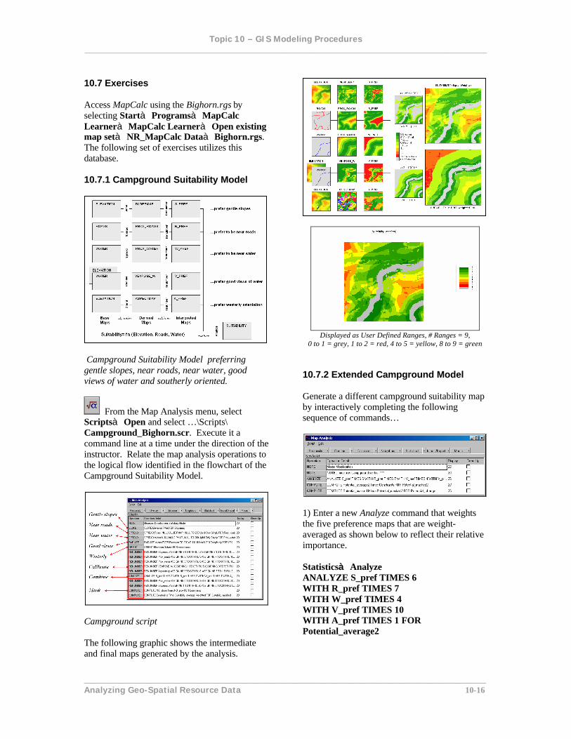
10.7 Exercises Access MapCalc using the Bighorn.rgs by selecting Startà Programsà MapCalc Learnerà MapCalc Learnerà Open existing map setà NR_MapCalc Dataà Bighorn.rgs. The following set of exercises utilizes this database. 10.7.1 Campground Suitability Model

Campground Suitability Model preferring gentle slopes, near roads, near water, good views of water and southerly oriented.

From the Map Analysis menu, select Scriptsà Open and select …\Scripts\ Campground_Bighorn.scr. Execute it a command line at a time under the direction of the instructor. Relate the map analysis operations to the logical flow identified in the flowchart of the Campground Suitability Model.

Campground script The following graphic shows the intermediate and final maps generated by the analysis.

Displayed as User Defined Ranges, # Ranges = 9,

0 to 1 = grey, 1 to 2 = red, 4 to 5 = yellow, 8 to 9 = green 10.7.2 Extended Campground Model Generate a different campground suitability map by interactively completing the following sequence of commands…

1) Enter a new Analyze command that weights the five preference maps that are weight-averaged as shown below to reflect their relative importance. Statisticsà Analyze ANALYZE S_pref TIMES 6 WITH R_pref TIMES 7 WITH W_pref TIMES 4 WITH V_pref TIMES 10 WITH A_pref TIMES 1 FOR Potential_average2



Note: be sure to press the “Add” button each time a new map and weight is entered. 2) Use the Compute command to mask the constrained areas. Overlayà Compute COMPUTE Potential_average2 Times Constraints FOR Suitability2_masked


0 to 1 = grey, 1 to 2 = red, 4 to 5 = yellow, 8 to 9 = green 3) Use Compute to compare the simple average and weighted-average maps. Overlayà Compute COMPUTE Suitability_masked Minus Suitability2_masked FOR Suitability_difference


-4 to -3 = red,0 to.001 = yellow 8 to 9 = green

10.7.3 Editing and Using Scripts

Click on the Macro button and select Note.

Enter a heading for the extended analysis. Click on the Macro button and select Pause. Then click and drag the Pause line to the top of the set of new command lines; place the Note line below it; and move the “…end of script” line to the bottom.

From the Map Analysis menu, select Scriptà Save As… and name the extended scrip Campground_Bighorn_extended.scr ___________________________

topic 10 gis modeling procedures - innovative gis

Documents