topic 4: flow analysis
TRANSCRIPT
Topic 4: Topic 4: Topic 4: Topic 4:
Flow AnalysisFlow AnalysisFlow AnalysisFlow Analysis
2008/3/7 \course\cpeg421-08s\Topic4.ppt 1
Flow AnalysisFlow AnalysisFlow AnalysisFlow Analysis
Some slides come from Prof. J. N.
Amaral ([email protected])

Topic 4: Flow AnalysisTopic 4: Flow AnalysisTopic 4: Flow AnalysisTopic 4: Flow Analysis
• Motivation
• Control flow analysis
2008/3/7 \course\cpeg421-08s\Topic4.ppt 2
• Dataflow analysis
• Advanced topics
Reading ListReading ListReading ListReading List
• Slides
• Dragon book: chapter 8.4, 8.5, Chapter 9
2008/3/7 \course\cpeg421-08s\Topic4.ppt 3
• Muchnick’s book: Chapter 7
• Other readings as assigned in class or
homework

Basic block
Program
Procedure
Interprocedural
Intraprocedural
Local
Flow analysis
Data flow analysis
Control flow analysis
Flow Analysis
2008/3/7 \course\cpeg421-08s\Topic4.ppt 4
• Control Flow Analysis ─ Determine control structure
of a program and build a Control Flow Graph.
• Data Flow analysis ─ Determine the flow of scalar
values and ceretain associated properties
• Solution to the Flow analysis Problem: propagation
of data flow information along a flow graph.

Code optimization - a program transformation that
preserves correctness and improves the performance
(e.g., execution time, space, power) of the input
program. Code optimization may be performed at
multiple levels of program representation:
Introduction to Code Introduction to Code Introduction to Code Introduction to Code OptimizationsOptimizationsOptimizationsOptimizations
2008/3/7 \course\cpeg421-08s\Topic4.ppt 5
multiple levels of program representation:
1. Source code
2. Intermediate code
3. Target machine code
Optimized vs. optimal - the term “optimized” is used to
indicate a relative performance improvement.

MotivationMotivationMotivationMotivation
S1: A 2 (def of A)
S2: B 10 (def of B)...
2008/3/7 \course\cpeg421-08s\Topic4.ppt 6
S3: C A + B determine if C is aconstant 12?
S4 Do I = 1, C
A[I] = B[I] + D[I-1]
...

Basic BlocksBasic BlocksBasic BlocksBasic Blocks
A basic block is a sequence of consecutive
intermediate language statements in which flow of
control can only enter at the beginning and leave at
the end.
2008/3/7 \course\cpeg421-08s\Topic4.ppt 7
Only the last statement of a basic block can be a branch statement and only the first statement of a basic block can be a target of a branch. However, procedure calls may need be treated with care within a basic block (Procedure call starts a new basic block)
the end.
(AhoSethiUllman, pp. 529)

Basic Block Basic Block Basic Block Basic Block Partitioning AlgorithmPartitioning AlgorithmPartitioning AlgorithmPartitioning Algorithm
1. Identify leader statements (i.e. the first statements of basic blocks) by using the following rules:
(i) The first statement in the program is a leader
(ii) Any statement that is the target of a branch statement is a leader (for most IL’s. these are label
2008/3/7 \course\cpeg421-08s\Topic4.ppt 8
statement is a leader (for most IL’s. these are label statements)
(iii) Any statement that immediately follows a branch or return statement is a leader
2. The basic block corresponding to a leader consists of the leader, and all statements up to but not including the next leader or up to the end of the program.

Example
beginprod := 0;i := 1;
The following code computes the inner product of two vectors.
(1) prod := 0(2) i := 1(3) t1 := 4 * i(4) t2 := a[t1](5) t3 := 4 * i
2008/3/7 \course\cpeg421-08s\Topic4.ppt 9
do beginprod := prod + a[i] * b[i]i = i+ 1;
endwhile i <= 20
end
(5) t3 := 4 * i(6) t4 := b[t3](7) t5 := t2 * t4(8) t6 := prod + t5(9) prod := t6(10) t7 := i + 1(11) i := t7(12) if i <= 20 goto (3)(13) …
Source code.
Three-address code.

Example
beginprod := 0;i := 1;
The following code computes the inner product of two vectors.
(1) prod := 0(2) i := 1(3) t1 := 4 * i(4) t2 := a[t1]
Rule (i)
2008/3/7 \course\cpeg421-08s\Topic4.ppt 10
i := 1;do begin
prod := prod + a[i] * b[i]i = i+ 1;
endwhile i <= 20
end
(4) t2 := a[t1](5) t3 := 4 * i(6) t4 := b[t3](7) t5 := t2 * t4(8) t6 := prod + t5(9) prod := t6(10) t7 := i + 1(11) i := t7(12) if i <= 20 goto (3)(13) …
Source code.
Three-address code.

Example
beginprod := 0;i := 1;
The following code computes the inner product of two vectors.
(1) prod := 0(2) i := 1(3) t1 := 4 * i(4) t2 := a[t1]
Rule (i)
Rule (ii)
2008/3/7 \course\cpeg421-08s\Topic4.ppt 11
i := 1;do begin
prod := prod + a[i] * b[i]i = i+ 1;
endwhile i <= 20
end
(4) t2 := a[t1](5) t3 := 4 * i(6) t4 := b[t3](7) t5 := t2 * t4(8) t6 := prod + t5(9) prod := t6(10) t7 := i + 1(11) i := t7(12) if i <= 20 goto (3)(13) …
Source code.
Three-address code.
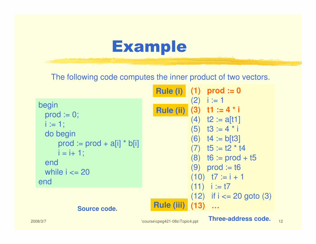
Example
beginprod := 0;i := 1;
The following code computes the inner product of two vectors.
(1) prod := 0(2) i := 1(3) t1 := 4 * i(4) t2 := a[t1]
Rule (i)
Rule (ii)
2008/3/7 \course\cpeg421-08s\Topic4.ppt 12
i := 1;do begin
prod := prod + a[i] * b[i]i = i+ 1;
endwhile i <= 20
end
(4) t2 := a[t1](5) t3 := 4 * i(6) t4 := b[t3](7) t5 := t2 * t4(8) t6 := prod + t5(9) prod := t6(10) t7 := i + 1(11) i := t7(12) if i <= 20 goto (3)(13) …Source code.
Three-address code.
Rule (iii)

Example
Basic Blocks:
(1) prod := 0(2) i := 1
(3) t1 := 4 * i(4) t2 := a[t1](5) t3 := 4 * i
B1
B2
2008/3/7 \course\cpeg421-08s\Topic4.ppt 13
Basic Blocks:(5) t3 := 4 * i(6) t4 := b[t3](7) t5 := t2 * t4(8) t6 := prod + t5(9) prod := t6(10) t7 := i + 1(11) i := t7(12) if i <= 20 goto (3)
(13) …B3

Transformations on Basic Blocks
• Structure-Preserving Transformations:
• common subexpression elimination
• dead code elimination
2008/3/7 \course\cpeg421-08s\Topic4.ppt 14
• dead code elimination
• renaming of temporary variables
• interchange of two independent adjacent statements
• Others …
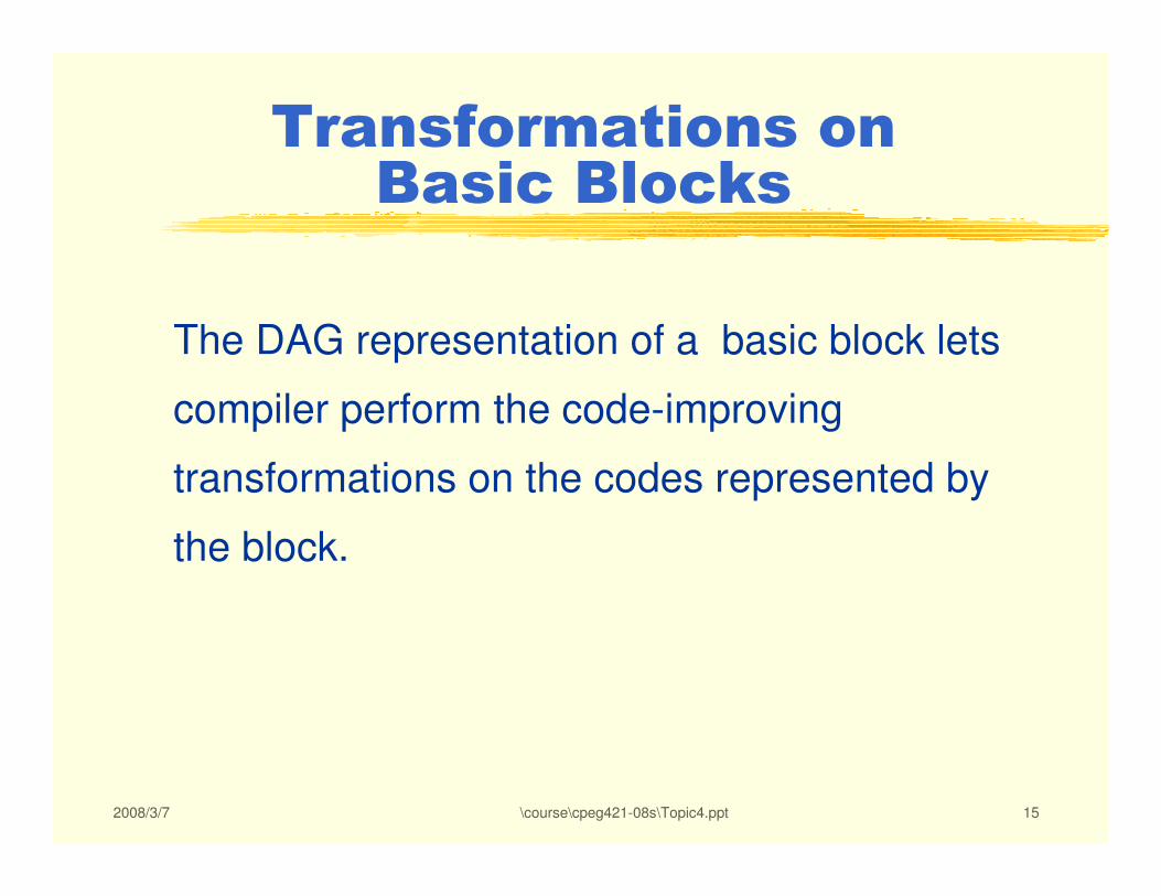
Transformations on Basic Blocks
The DAG representation of a basic block lets
compiler perform the code-improving
2008/3/7 \course\cpeg421-08s\Topic4.ppt 15
transformations on the codes represented by
the block.

Transformations on Basic Blocks
Algorithm of the DAG construction for a basic block
• Create a node for each of the initial values of the variables in
the basic block
• Create a node for each statement s, label the node by the
2008/3/7 \course\cpeg421-08s\Topic4.ppt 16
• Create a node for each statement s, label the node by the
operator in the statement s, and attach the list of variables for
which it is the last definition in the basic block.
• The children of a node N are those nodes corresponding to
statements that are last definitions of the operands used in the
statement associated with node N.
Tiger book pp533

An Example of Constructing the DAG
Step (1): create node 4 and i0Step (2): create node *
Step (3): attach identifier t1
*t1
i04
t1: = 4*i
t2 := a[t1]
t3 := 4*i
2008/3/7 \course\cpeg421-08s\Topic4.ppt 17
Step (1): create nodes labeled [], a
Step (2): find previously node(t1)
Step (3): attach label
Here we determine that:
node (4) was created
node (i) was created
node (*) was created
i04
*t1,t3
i04
[ ]t2
a0
just attach t3 to node *

Example of Common Subexpression Elimination
(1) a:= b + c
(2) b:= a – d
(3) c:= b + c
(4) d:= a - d
a:= b + c
b:= a – d
c:= b + c
d:= b
+
+
-
b0c0
d0
c
b,d
a
2008/3/7 \course\cpeg421-08s\Topic4.ppt 18
Detection:
Common subexpressions can be detected by noticing, as a new node m is
about to be added, whether there is an existing node n with the same children, in the same order, and with the same operator.
if so, n computes the same value as m and may be used in its place.
(4) d:= a - d b0c0
If a node N represents a common subexpression, N has more than
one attached variables in the DAG.

Example of Dead Code Elimination
if x is never referenced after the statement x = y+z, the
statement can be safely eliminated.
2008/3/7 \course\cpeg421-08s\Topic4.ppt 19

Example of Renaming Temporary Variables
(1) t := b + c (1) u := b + crename
+t
+u
Change (rename)
2008/3/7 \course\cpeg421-08s\Topic4.ppt 20
b0 c0 b0 c0label
a code in which each temporary is defined only once is called
a single assignment form.
if there is an statement t := b + c, we can change it to u := b + cand change all uses of t to u.

Example of Interchange of Statements
t1 := b + ct2 := x + y
+t1
b0 c0
+t2
x0 y0
2008/3/7 \course\cpeg421-08s\Topic4.ppt 21
Observation:
We can interchange the statements without affecting the value of the block if and only if neither x nor y is t1 and neither b nor c is t2, i.e. we have two DAG subtrees.

Example of Algebraic Transformations
Arithmetic Identities:
x + 0 = 0 + x = x
x – 0 = x
x * 1 = 1 * x = x
x / 1 = x
- Replace left-hand side with
Reduction in strength:
x ** 2 = x * x
2.0 * x = x + x
x / 2 = x * 0.5
- Replace an expensive
2008/3/7 \course\cpeg421-08s\Topic4.ppt 22
- Replace left-hand side with simples right hand side.
Associative/Commutative laws
x + (y + z) = (x + y) + z
x + y = y + x
- Replace an expensive operator with a cheaper one.
Constant folding
2 * 3.14 = 6.28
-Evaluate constant expression at compile time`

Control Flow Graph (CFG)Control Flow Graph (CFG)Control Flow Graph (CFG)Control Flow Graph (CFG)
A control flow graph (CFG), or simply a flow graph, is a directed multigraph in which the nodes are basic blocks and edges represent flow of control (branches or fall-through execution).
• The basic block whose leader is the first statement is called the initial node or start node
2008/3/7 \course\cpeg421-08s\Topic4.ppt 23
node or start node
• There is a directed edge from basic block B1 to basic B2 in the CFG if:
(1) There is a branch from the last statement of B1 to the first
statement of B2, or
(2) Control flow can fall through from B1 to B2 because B2
immediately follows B1, and B1 does not end with an
unconditional branch

Example
(1) prod := 0(2) i := 1
(3) t1 := 4 * i(4) t2 := a[t1]
B1
B2
Rule (2)
Control Flow Graph:
B1
2008/3/7 \course\cpeg421-08s\Topic4.ppt 24
(4) t2 := a[t1](5) t3 := 4 * i(6) t4 := b[t3](7) t5 := t2 * t4(8) t6 := prod + t5(9) prod := t6(10) t7 := i + 1(11) i := t7(12) if i <= 20 goto (3)
(13) …B3
Rule (1)Rule (2)
B2
B3

CFGs are Multigraphs
Note: there may be multiple edges from one basic block to another in a CFG.
Therefore, in general the CFG is a multigraph.
The edges are distinguished by their condition labels.
2008/3/7 \course\cpeg421-08s\Topic4.ppt 25
The edges are distinguished by their condition labels.
A trivial example is given below:
[101] . . .
[102] if i > n goto L1 Basic Block B1
[103] label L1:
[104] . . . Basic Block B2
False True

Identifying loops
Question: Given the control flow graph of a procedure, how can we identify loops?
2008/3/7 \course\cpeg421-08s\Topic4.ppt 26
Answer: We use the concept of dominance.

DominatorsDominatorsDominatorsDominators
Node (basic block) D in a CFG dominates node N if
every path from the start node to N goes through D.
We say that node D is a dominator of node N.
2008/3/7 \course\cpeg421-08s\Topic4.ppt 27
Define DOM(N) = set of node N’s dominators, or the
dominator set for node N.
Note: by definition, each node dominates itself i.e., N ∈∈∈∈ DOM(N).

Definition: Let G = (N, E, s) denote a flowgraph.
and let n, n’ ∈ N.
1. n dominates n’, written n ≤ n’ :
each path from s to n’ contains n.
Domination RelationDomination RelationDomination RelationDomination Relation
2008/3/7 \course\cpeg421-08s\Topic4.ppt 28
each path from s to n’ contains n.
2. n properly dominates n’, written n < n’ :
n ≤ n’ and n ≠ n’.
3. n directly (immediately) dominates n’, written n <d n’:
n < n’ and
there is no m ∈ N such that n < m < n’.
4. DOM(n) := {n’ : n’ ≤ n} is the set of dominators of n.
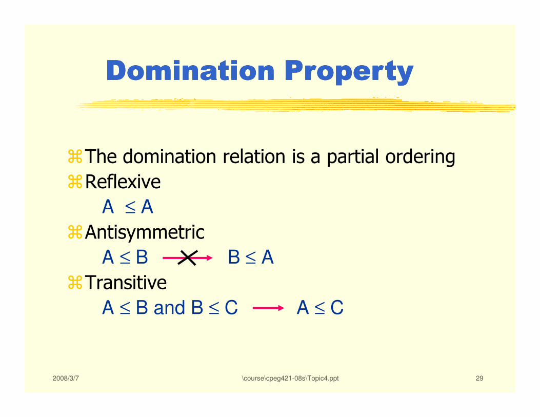
�The domination relation is a partial ordering
�Reflexive
A ≤ A
Domination PropertyDomination PropertyDomination PropertyDomination Property
2008/3/7 \course\cpeg421-08s\Topic4.ppt 29
A ≤ A
�Antisymmetric
A ≤ B B ≤ A
�Transitive
A ≤ B and B ≤ C A ≤ C

Computing DominatorsComputing DominatorsComputing DominatorsComputing Dominators
Observe: if a dominates b, then
• a = b, or
• a is the only immediate predecessor of b, or
• b has more than one immediate predecessor, all
2008/3/7 \course\cpeg421-08s\Topic4.ppt 30
• b has more than one immediate predecessor, all
of which are dominated by a.
DOM(b) = {b} U ∩ DOM(p)p ∈∈∈∈ pred(b)
Quiz: why here is the intersection
operator instead of the union?

Domination relation:
An ExampleAn ExampleAn ExampleAn Example
1
2
3
S{ (1, 1), (1, 2), (1, 3), (1, 4) …
(2, 3), (2, 4), …(2, 10)
}
Direct domination:
2008/3/7 \course\cpeg421-08s\Topic4.ppt 31
4
5
6 7
8
9
10
Direct domination:
DOM:
1 <d 2, 2 <d 3, …
DOM(1) = {1}DOM(2) = {1, 2}DOM(10) = {1, 2, 10}…
DOM(8) ? DOM(8) ={ 1,2,3,4,5,8}

QuestionQuestionQuestionQuestion
Assume node m is an immediate dominator of a node n, is m necessarily an immediate predecessor of n
1
2
3
4
S
2008/3/7 \course\cpeg421-08s\Topic4.ppt 32
immediate predecessor of nin the flow graph?
Answer: NO!Example:
consider
nodes 5 and
8.
4
5
6 7
8
9
10
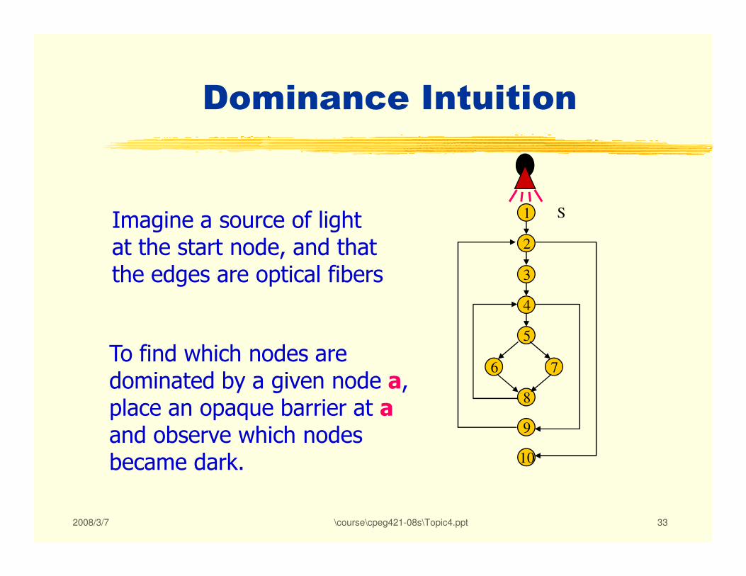
Dominance Intuition
1
2
3
SImagine a source of lightat the start node, and thatthe edges are optical fibers
2008/3/7 \course\cpeg421-08s\Topic4.ppt 33
4
5
6 7
8
9
10
To find which nodes are dominated by a given node a, place an opaque barrier at aand observe which nodes became dark.

Dominance Intuition
1
2
3
SThe start node dominates all nodes in the flowgraph.
2008/3/7 \course\cpeg421-08s\Topic4.ppt 34
4
5
6 7
8
9
10
Dominance Intuition
1
2
3
S
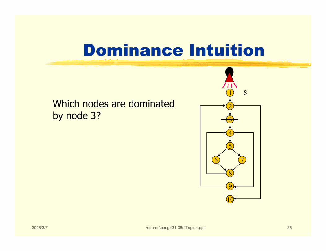
Which nodes are dominatedby node 3?
2008/3/7 \course\cpeg421-08s\Topic4.ppt 35
4
5
6 7
8
9
10

Dominance Intuition
1
2
3
S
Which nodes are dominatedby node 3?
2008/3/7 \course\cpeg421-08s\Topic4.ppt 36
4
5
6 7
8
9
10
Node 3 dominates nodes3, 4, 5, 6, 7, 8, and 9.
Dominance Intuition
1
2
3
S
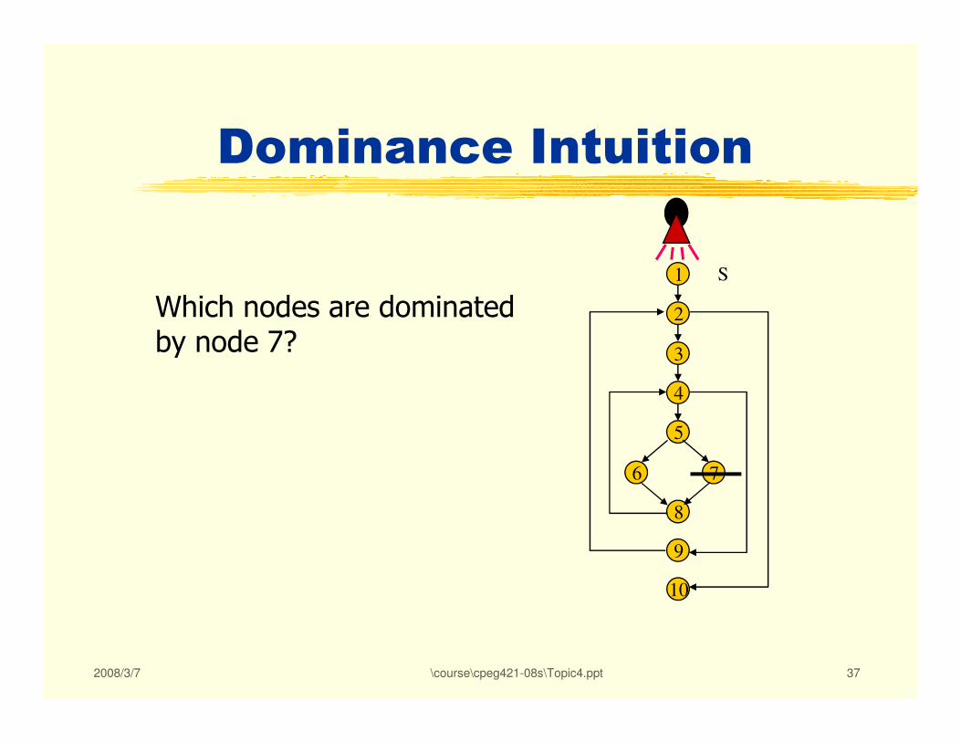
Which nodes are dominatedby node 7?
2008/3/7 \course\cpeg421-08s\Topic4.ppt 37
4
5
6 7
8
9
10

Dominance Intuition
1
2
3
S
Which nodes are dominatedby node 7?
2008/3/7 \course\cpeg421-08s\Topic4.ppt 38
4
5
6 7
8
9
10
Node 7 only dominatesitself.

Immediate Dominators and Immediate Dominators and Immediate Dominators and Immediate Dominators and Dominator TreeDominator TreeDominator TreeDominator Tree
Node M is the immediate dominator of node N ==>
Node M must be the last dominator of N on any path
from the start node to N.
2008/3/7 \course\cpeg421-08s\Topic4.ppt 39
Therefore, every node other than the start node must
have a unique immediate dominator (the start node has
no immediate dominator.)
What does this mean ?
A Dominator Tree
A dominator tree is a useful way to represent the dominance relation.
In a dominator tree the start node s is the root,
2008/3/7 \course\cpeg421-08s\Topic4.ppt 40
In a dominator tree the start node s is the root, and each node d dominates only its descendants in the tree.

Dominator Tree (Example)Dominator Tree (Example)Dominator Tree (Example)Dominator Tree (Example)
1
2
3
4
S
1
2
10
2008/3/7 \course\cpeg421-08s\Topic4.ppt 41
4
5
6 7
8
9
10
3
4
5
7 86
9
10
A flowgraph (left) and its dominator tree (right)

Natural LoopsNatural LoopsNatural LoopsNatural Loops
• Back-edges - an edge (B, A), such that
A < B (A properly dominates B).
• Header --A single-entry node which dominates all
2008/3/7 \course\cpeg421-08s\Topic4.ppt 42
nodes in a subgraph.
• Natural loops: given a back edge (B, A), a natural
loop of (B, A) with entry node A is the graph: A
plus all nodes which is dominated by A and can
reach B without going through A.

Find Natural Loops
start One way to find natural loops is:
1) find a back edge (b,a)
2008/3/7 \course\cpeg421-08s\Topic4.ppt 43
a
b
2) find the nodes that are dominated by a.
3) look for nodes that can reachb among the nodes dominatedby a.
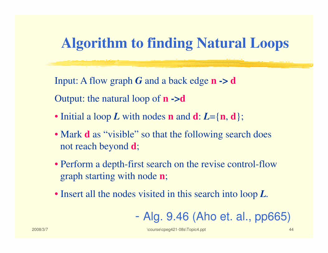
Algorithm to finding Natural Loops
Input: A flow graph G and a back edge n -> d
Output: the natural loop of n ->d
• Initial a loop L with nodes n and d: L={n, d};
2008/3/7 \course\cpeg421-08s\Topic4.ppt 44
- Alg. 9.46 (Aho et. al., pp665)
• Mark d as “visible” so that the following search does
not reach beyond d;
• Perform a depth-first search on the revise control-flow
graph starting with node n;
• Insert all the nodes visited in this search into loop L.
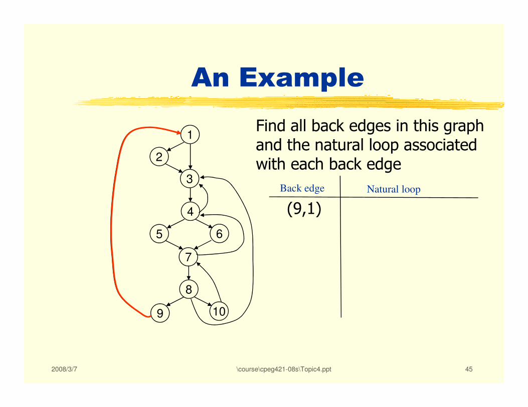
An Example
Find all back edges in this graphand the natural loop associated with each back edge
1
2
3
(9,1)
Back edge Natural loop
2008/3/7 \course\cpeg421-08s\Topic4.ppt 45
4
7
5 6
8
9 10
(9,1)

1
2
3
An Example
Find all back edges in this graphand the natural loop associated with each back edge
(9,1) Entire graph
Back edge Natural loop
2008/3/7 \course\cpeg421-08s\Topic4.ppt 46
4
7
5 6
8
9 10
(9,1) Entire graph
1
2
3
An Example
Find all back edges in this graphand the natural loop associated with each back edge
(9,1) Entire graph
Back edge Natural loop
2008/3/7 \course\cpeg421-08s\Topic4.ppt 47
4
7
5 6
8
9 10
(9,1) Entire graph
(10,7)

1
2
3
An Example
Find all back edges in this graphand the natural loop associated with each back edge
(9,1) Entire graph
Back edge Natural loop
2008/3/7 \course\cpeg421-08s\Topic4.ppt 48
4
7
5 6
8
9 10
(9,1) Entire graph
(10,7)

1
2
3
An Example
Find all back edges in this graphand the natural loop associated with each back edge
(9,1) Entire graph
Back edge Natural loop
2008/3/7 \course\cpeg421-08s\Topic4.ppt 49
4
7
5 6
8
9 10
(9,1) Entire graph
(10,7) {7,8,10}

1
2
3
An Example
Find all back edges in this graphand the natural loop associated with each back edge
(9,1) Entire graph
Back edge Natural loop
2008/3/7 \course\cpeg421-08s\Topic4.ppt 50
4
7
5 6
8
9 10
(9,1) Entire graph
(10,7) {7,8,10}
(7,4)

1
2
3
An Example
Find all back edges in this graphand the natural loop associated with each back edge
Back edge Natural loop
2008/3/7 \course\cpeg421-08s\Topic4.ppt 51
4
7
5 6
8
9 10
(9,1) Entire graph
(10,7) {7,8,10}
(7,4)
1
2
3
An Example
Find all back edges in this graphand the natural loop associated with each back edge
Back edge Natural loop
2008/3/7 \course\cpeg421-08s\Topic4.ppt 52
4
7
5 6
8
9 10
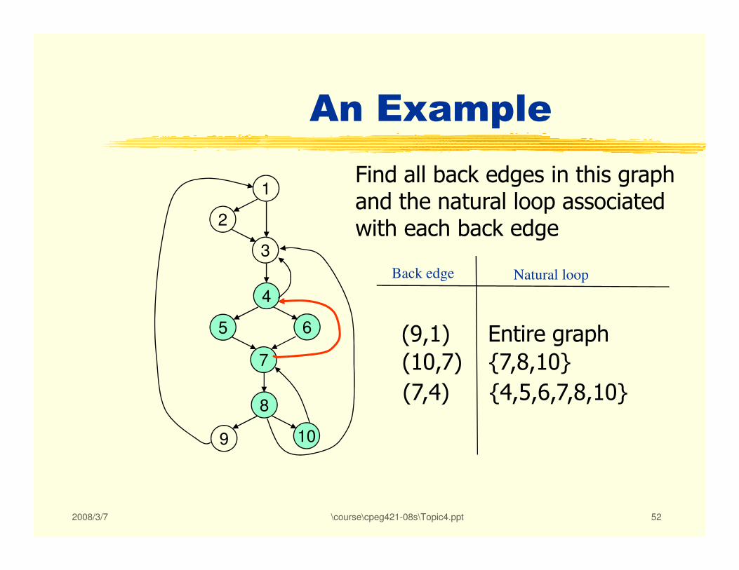
(9,1) Entire graph
(10,7) {7,8,10}
(7,4) {4,5,6,7,8,10}

1
2
3
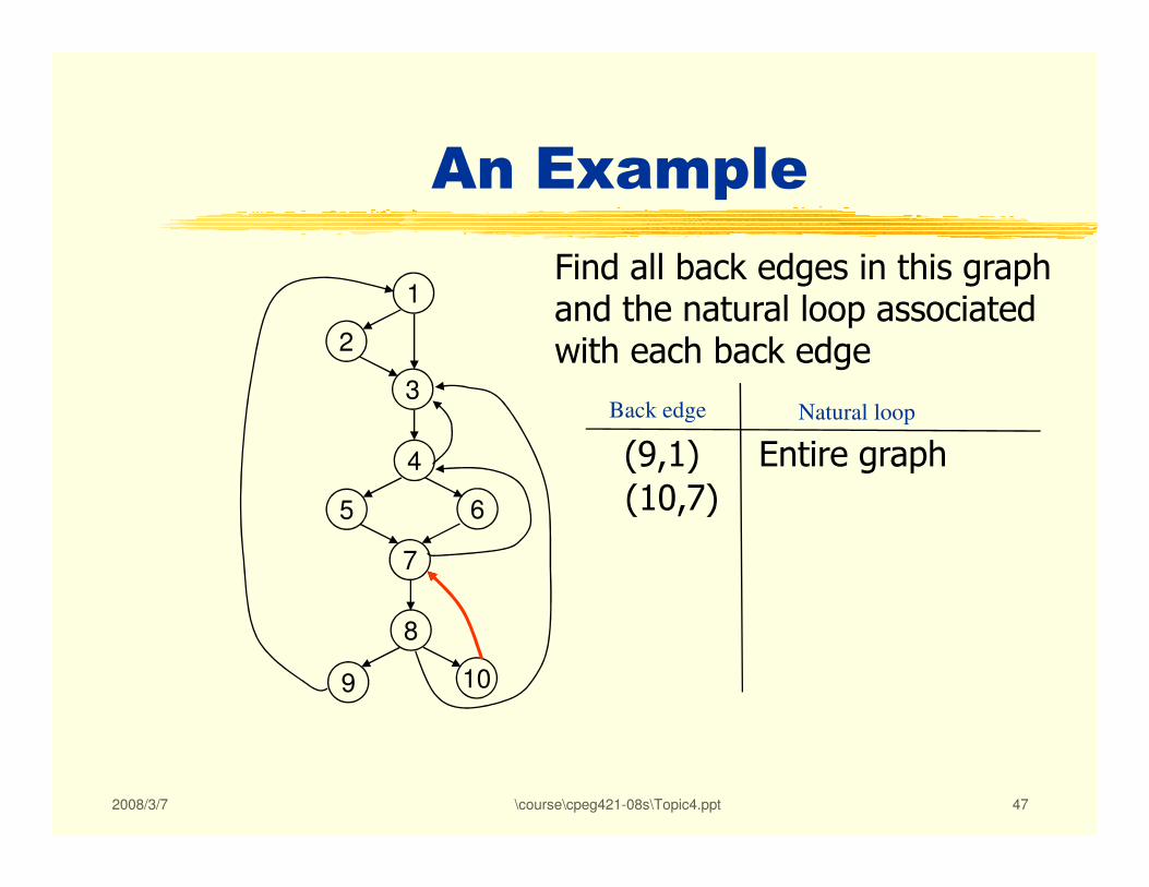
An Example
Find all back edges in this graphand the natural loop associated with each back edge
Back edge Natural loop
2008/3/7 \course\cpeg421-08s\Topic4.ppt 53
4
7
5 6
8
9 10
(9,1) Entire graph
(10,7) {7,8,10}
(7,4) {4,5,6,7,8,10}
(8,3)

1
2
3
An Example
Find all back edges in this graphand the natural loop associated with each back edge
Back edge Natural loop
2008/3/7 \course\cpeg421-08s\Topic4.ppt 54
4
7
5 6
8
9 10
(9,1) Entire graph
(10,7) {7,8,10}
(7,4) {4,5,6,7,8,10}
(8,3)
1
2
3
An Example
Find all back edges in this graphand the natural loop associated with each back edge
Back edge Natural loop
2008/3/7 \course\cpeg421-08s\Topic4.ppt 55
4
7
5 6
8
9 10
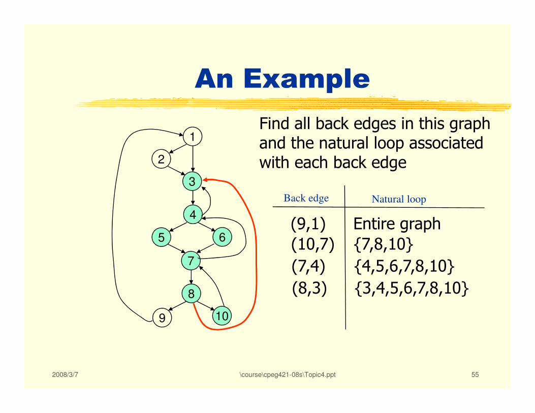
(9,1) Entire graph
(10,7) {7,8,10}
(7,4) {4,5,6,7,8,10}
(8,3) {3,4,5,6,7,8,10}

1
2
3
An Example
Find all back edges in this graphand the natural loop associated with each back edge
Back edge Natural loop
2008/3/7 \course\cpeg421-08s\Topic4.ppt 56
4
7
5 6
8
9 10
(9,1) Entire graph
(10,7) {7,8,10}
(7,4) {4,5,6,7,8,10}
(8,3) {3,4,5,6,7,8,10}
(4,3)

1
2
3
An Example
Find all back edges in this graphand the natural loop associated with each back edge
Back edge Natural loop
2008/3/7 \course\cpeg421-08s\Topic4.ppt 57
4
7
5 6
8
9 10
(9,1) Entire graph
(10,7) {7,8,10}
(7,4) {4,5,6,7,8,10}
(8,3) {3,4,5,6,7,8,10}
(4,3)

1
2
3
An Example
Find all back edges in this graphand the natural loop associated with each back edge
Back edge Natural loop
2008/3/7 \course\cpeg421-08s\Topic4.ppt 58
4
7
5 6
8
9 10
(9,1) Entire graph
(10,7) {7,8,10}
(7,4) {4,5,6,7,8,10}
(8,3) {3,4,5,6,7,8,10}
(4,3) {3,4,5,6,7,8,10}
Reducible Flow GraphsReducible Flow GraphsReducible Flow GraphsReducible Flow Graphs
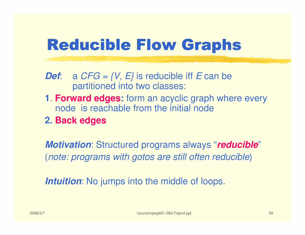
Def: a CFG = {V, E} is reducible iff E can be partitioned into two classes:
1. Forward edges: form an acyclic graph where every node is reachable from the initial node
2. Back edges
2008/3/7 \course\cpeg421-08s\Topic4.ppt 59
2. Back edges
Motivation: Structured programs always “reducible”
(note: programs with gotos are still often reducible)
Intuition: No jumps into the middle of loops.

Step1: compute “dom” relation
Step2: identify all back edges
Step3: remove all back edges and derive G’
How to check if a graph G is reducible?
2008/3/7 \course\cpeg421-08s\Topic4.ppt 60
Step3: remove all back edges and derive G’
Step4: check if G’ is acyclic
Example: 1
2 3
Bad cycle: can be entered from 2 different places
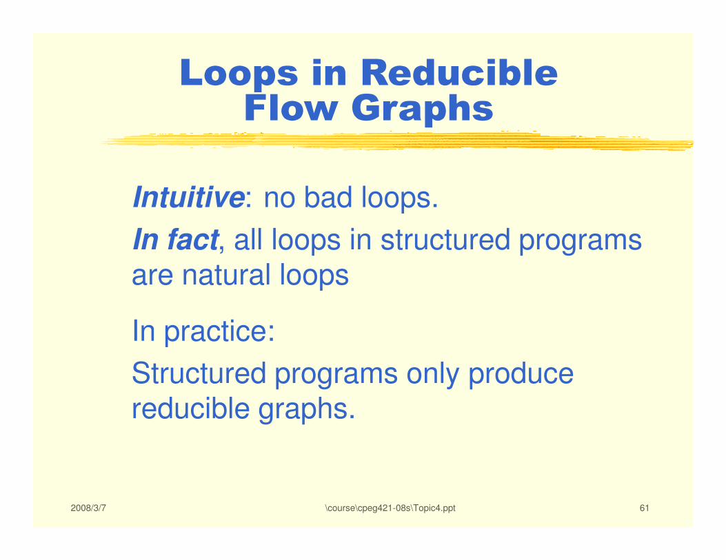
Intuitive: no bad loops.
In fact, all loops in structured programs are natural loops
Loops in Reducible Flow Graphs
2008/3/7 \course\cpeg421-08s\Topic4.ppt 61
are natural loops
In practice:
Structured programs only produce reducible graphs.

More About Loops
� Read the following slides and think?
2008/3/7 \course\cpeg421-08s\Topic4.ppt 62
Region and Loop
A region is a set of nodes N that include a header with the
following properties:
(i) the header must dominate all the nodes in the region;
(ii) All the edges between nodes in N are in the region
2008/3/7 \course\cpeg421-08s\Topic4.ppt 63
(ii) All the edges between nodes in N are in the region
(except for some edges that enter the header);
A loop is a special region that has the following additional
properties:
(i) it is strongly connected;
(ii) All back edges to the header are included in the loop;

Loops in Control Flow GraphsLoops in Control Flow GraphsLoops in Control Flow GraphsLoops in Control Flow Graphs
Motivation: Programs spend more time in loops, so there is a larger payoff from optimizations that exploit loop structure e.g., loop-invariant code motion, software pipelining, etc.
2008/3/7 \course\cpeg421-08s\Topic4.ppt 64
Basic idea: Identify regions (subgraphs) of the CFG that correspond to program loops. Use a general approach based on analyzing graph-theoretical properties of the CFG - uniform treatment for program loops written using different loop structures (e.g. while, for) and loops constructed out of goto’s.

Relation of Flowgraph and Loop:
A Definition
A strongly-connected component (SCC) of a flowgraph G = (N, E, s) is a subgraph
G’ = (N’, E’, s’) in which there is a path
from each node in N’ to every node in N’.
2008/3/7 \course\cpeg421-08s\Topic4.ppt 65
A strongly-connected component G’ = (N’, E’, s’)of a flowgraph G = (N, E, s) is a loop with entry s’if s’ dominates all nodes in N’.
from each node in N’ to every node in N’.
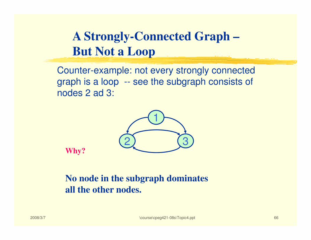
Counter-example: not every strongly connected
graph is a loop -- see the subgraph consists of
nodes 2 ad 3:
1
A Strongly-Connected Graph –
But Not a Loop
2008/3/7 \course\cpeg421-08s\Topic4.ppt 66
1
2 3Why?
No node in the subgraph dominates
all the other nodes.