towards a unified description of quantum liquid and
TRANSCRIPT

HAL Id: tel-01915952https://tel.archives-ouvertes.fr/tel-01915952
Submitted on 8 Nov 2018
HAL is a multi-disciplinary open accessarchive for the deposit and dissemination of sci-entific research documents, whether they are pub-lished or not. The documents may come fromteaching and research institutions in France orabroad, or from public or private research centers.
L’archive ouverte pluridisciplinaire HAL, estdestinée au dépôt et à la diffusion de documentsscientifiques de niveau recherche, publiés ou non,émanant des établissements d’enseignement et derecherche français ou étrangers, des laboratoirespublics ou privés.
Towards a unified description of quantum liquid andcluster states in atomic nuclei within the relativistic
energy density functional frameworkPetar Marević
To cite this version:Petar Marević. Towards a unified description of quantum liquid and cluster states in atomic nucleiwithin the relativistic energy density functional framework. Nuclear Theory [nucl-th]. Université ParisSaclay (COmUE), 2018. English. NNT : 2018SACLS358. tel-01915952

*
NN
T:2
018S
AC
LS35
8
Towards a unified description ofquantum liquid and cluster states
in atomic nuclei within therelativistic energy density
functional frameworkThese de doctorat de l’Universite Paris-Saclay
preparee a l’Universite Paris-Sud
Ecole doctorale n576 Particules, Hadrons, Energie, Noyau, Instrumentation, Imagerie,Cosmos et Simulation (PHENIICS)
Specialite de doctorat : Structure et reactions nucleaires
These presentee et soutenue a Orsay, le 2 octobre 2018, par
PETAR MAREVIC
Composition du Jury :
M. Peter SchuckDirecteur de Recherche Emerite, IPN Orsay, France President
M. Luis RobledoProfesseur, Autonomous University of Madrid, Spain Rapporteur
M. Matko MilinProfesseur, University of Zagreb, Croatia Rapporteur
M. Nicolas SchunckCharge de Recherche, LLNL Livermore, the United States Examinateur
M. Dario VretenarProfesseur, University of Zagreb, Croatia Examinateur
M. Elias KhanProfesseur, IPN Orsay, Universite Paris-Saclay, France Directeur de these
M. Jean-Paul EbranCharge de Recherche, CEA, DAM, DIF, France Co-directeur de these


Acknowledgements
Messieurs les officiers, je vous remercie.
Toreador Escamillo, Act 2, Carmen by G. Bizet
Le doctorat dure trois ans, un peu comme l’amour1. The past three years have ar-guably been, both professionally and personally, the most eventful and intense period ofmy life. While I hope that the manuscript before you will remain as a lasting evidence ofthe work done during this period, some of the interesting stories and events - that seem tobe of an almost equal importance in forming of a young scientist and person - will likelyremain untold. In paragraphs that follow, however, I would like to express my gratitudeto people that partook in some of them and that have thereby, in one way or another,influenced my life and work during this exciting journey.
Time and place: Oct31 2015, CDG Airport, Paris. My level of French: Bonjour, merci.Luckily, my thesis advisor Jean-Paul was there, together with his wife and children, towelcome me on my arrival to France. Even though (as he will reveal publicly years later,during my thesis defense) I did not sufficiently appreciate the food that he himself cookedfor me on the day, I will always stay grateful for his presence and assistance during thosefirst weeks in a completely new environment. Having such a talented physicist by myside during this thesis was a real privilege and it provided me with a great amount ofconfidence in my everyday work. Moreover, I feel impelled to say that Jean-Paul’s (pre-dominantly) kind personality, uncommon sense of humor, and cheerful spirit made me- as time passed by - start considering him as less of a boss and more of an older bro(though, to be fair, the one who is living abroad and can be encountered only on rarefamily gatherings). Furthermore, thanks are due to my other advisor, Elias (Emranuzza-man) Khan, a non-owner of the Researchgate profile, Laurate of the CNRS Silver Medal2016, and a skillful basketball player (verified by yours truly on an usually hot and tiringday in Perpignan, summer 2016). Even though Croatia virtually never managed to beatFrance in any of the sports competitions that we permanently bantered about2, it wasa real pleasure to work under Elias, both for his relaxed but effective approach to workand for always having my guy in the university administration who can help me resolveany bureaucratic struggle. The extent of my gratitude to Tamara Niksic, my mastersthesis advisor and PhD advisor in charge, cannot be overstated. Tamara’s competence,calmness, and dedication to work remain a source of perpetual inspiration for me, while
1For more details on the latter subject an interested reader is referred to F. Beigbeder, L’amour duretrois ans, Editions Grasset & Fasquelle (1997).
2It was not a penalty.
iii

iv
countless e-mail and Skype exchanges that we had over the past years testify to the majorrole she played in making of this thesis and in making of this physicist.
I would like to extend my sincere gratitude to all the members of the committee.Firstly, many thanks to Peter Schuck, an experienced master of the field, for presidingover the committee and for continuously reminding me to keep an eye on the Hoyle state.Special thanks go to two referees, Luis Robledo and Matko Milin, who authorized for thethesis defense to happen in the first place. Luis’ extraordinary contributions to the fieldof beyond mean-field models remain one of my favorite scientific reads and they indeedrepresents an important pillar of the present thesis. While Matko’s experimental work onclusters remains somewhat less transparent to my theoretical mind, his unusually kindpersonality and deep physics knowledge - dating in my personal calendar as far back asGeneral Physics classes in 2011 - had a very strong influence on my scientific career.Finally, thanks are due to two examiners. I am grateful to Nicolas Schunck for travelingfrom the US to take part in my committee and, even more, for enabling my future travelto the US to take part in our common project. Thanks to Dario Vretenar, for takinginterest and care in my professional development and for using his immense knowledgeand experience to better the research that I try to perform. Having my work verified bysuch an exceptional group of physicists was both honoring and humbling experience.
During the past three years I had a privilege of working at two of the best nuclearphysics institutions in France. I would like to thank the people of my laboratory inBruyeres-le-Chatel for taking a Croatian guy among their ranks. Je suis navre que nousn’ayons pas pu passer plus de temps ensemble et j’espere que le futur nous en offriral’opportunite. On the other hand, I am immensely grateful to the entire scientific, ad-ministrative, and informatics staff of IPN Orsay for welcoming me in their nest andallowing me to make our lab my second home (which was, during the last months ofwriting this manuscript, admittedly true also in a literal sense). Dear Bira, David R.,Denis, Giai, Guillaume, Jean-Philippe, and Marcella, it was a pleasure to share theorycorridor and CESFO table with you, and I hope to see you all around in the near future.Special thanks go to the funniest member of the group, Paolo, for numerous cheerful andsilly conversations we had, as well as to the head of the group Michael, for making me afull-fledged group member and helping me with hardware issues prior to my long postdocinterview. Thanks to our group secretary Valerie, pour son aide toujours aimable et pourm’avoir aide a organiser mon pot de these.
Upon my arrival to IPN, I had to take the least attractive desk in the office 101a. Iwould like to thank Noel for letting me inherit his desk after his departure, as well as forintroducing me to and sharing many drinks at my favorite Parisian bar. I raise a cup ofCafe Raoul to Raphael, my travel companion to York and Galveston and an extraordi-narily bright young mind: it was a real pleasure to share an office, advisors, and an officialthesis title with him. I wish the best of luck to younger PhD students that I am leavingbehind at the battlefield: Antoine (look down!), David D., Hasim, and Melih. Significantamount of luck will also be needed by Jean-Paul’s remaining students - a new apprenticeKilian, whose driving and translation services were highly appreciated, and Julien, whomI’ve shared rooms with on our Gogny adventure in Madrid. I am grateful to IPN col-leagues and friends that I have spent numerous entertaining out-of-the-office hours with:the tressette master Alice, data scientist, drummer and Nature Physics author Aurelie,my first PRL co-author and the most stylish guy of IPN Clement, my tattooed Slav-sisJana, our salsa instructor Liss, as well as the vigilante hero Olivier, the Pheniicsman. Thepast three years were cheerful largely due to the presence of my dear friend and amouretteAnastasia, whom I shared a million of laughter-filled adventures with. Naturally, she was

v
particularly thrilled that I also shared my amazing friend Marc with her, and all three ofus are very excited about the upcoming Greek wedding in the summer of 2019. Specialmention goes to my meanest friend Florent, who is - let’s face it - much better volleyballthan a beer pong player. I am grateful for his not-so-kind guidance through the hell ofFrench language and bureaucracy, many late afternoon sandwich expeditions, and morethan anything for throwing the best birthday parties I have ever seen.
Spending mid-twenties in Paris is arguably not the worst destiny that can fall upon ayoung human being, and I was additionally blessed with the opportunity to travel ratherregularly over the past three years. Naming all of the people who made my time inParis and abroad pleasant would surely be an impossible task. Nevertheless, I wouldlike to give special thanks to Ariel, Alessandra, Benjamin, Dinko, Giulia, Luka, Niki,Pierre, Robert, and Xixi, for entertaining and precious time we spent together. A hugeshout-out and 100% thanks to my Croatian gang - Jure, Marko, Matija, Pave, and Sasa- for our exciting yearly eurotrips and for their warm welcomes every time I would getback home to Zagreb. Special mention goes to the Losos department of the gang, whovisited Paris for my defense and honored me with a captain armband to lead them inour Parisian adventures. My Croatian roommate (Cimer) of three years and, to use hismother’s words, almost a brother Branimir stayed close to me despite the Atlantic thatis currently separating us. 6161 thanks are due to him and his wife Lauren for travelingfrom DC to Paris to witness my defense. Somewhere along the way I was lucky enoughto stumble upon my dude and brave warrior Basak, whose gentle and (overly) pleasantcompany, particularly when there was a sh*tty pizza to share, made my mind calm andmy time unusually joyful.
There are people that may seem peripheral to the uninformed observer, but deep in-side, at the very absolute minimum of your potential energy surface, you just know thatyou should acknowledge them. To start with, I want to thank all of my French languageteachers, for largely enhancing my survival odds in this wild world. Some of my happiesthours were spent in Hurling Pub of the 5th arrondissement, at the bar or in front of thedartboard, and it is largely due to the two of the coolest bartenders. Furthermore, I oc-casionally enjoyed very tasteful pastries at the bakery of Orsay RERB station, preparedby an anonymous baker who always appeared to me as someone who once agreed to jumpin for a friend-baker that had an emergency but then, by a weird twist of fate, had tostay ever since. Special recognition goes to the anonymous referee of my first first-authorpaper, whose insightful remark Results are very interesting (...). However, the authorsare overoptimistic and the overall tone should be lowered probably strikes a general chordmore loudly than I would be willing to admit.
Finally, I want to thank my entire family, for tolerating and supporting a family blacksheep who is interested in studying some weird stuff that no sane person cares about.To my mom and dad, for deciding it was a good idea to have and raise one mischievousboy who grew up to become a doctor. To my sister and my brother in law, for makingtheir home mine whenever I needed so. And to my sweet nephews Boris and Dino, forperiodically reminding about the things in life that really matter.
In the end, I thank you, my dear reader, for taking your precious time to read thismanuscript. I wish you a very pleasant journey through the realm of breaking and restor-ing symmetries, and may your personal symmetries never need to be restored.
Orsay, October 26, 2018.


”The ponnies run, the girls are youngThe odds are there to beat.
You win a while and then it’s doneYour little winning streak.
And summoned now to dealWith your invincible defeat.
You live your life as if it’s realA thousand kisses deep.”
L. Cohen, “A Thousand Kisses Deep“


Contents
An Overture 1
I Theoretical Framework 9
1 The Nuclear Energy Density Functional Method 11
1.1 Relativistic Mean-Field Theory . . . . . . . . . . . . . . . . . . . . . . . 13
1.1.1 Basic Building Blocks of the RMF Theory . . . . . . . . . . . . . 13
1.1.2 The DD-PC1 Effective Interaction . . . . . . . . . . . . . . . . . . 15
1.1.3 The Separable Pairing Force . . . . . . . . . . . . . . . . . . . . . 20
1.2 Relativistic Hartree-Bogoliubov Model . . . . . . . . . . . . . . . . . . . 22
1.2.1 The Independent Quasiparticle Picture . . . . . . . . . . . . . . . 22
1.2.2 Relativistic Hartree-Bogoliubov Equation . . . . . . . . . . . . . . 24
1.2.3 Constrained RHB Calculation . . . . . . . . . . . . . . . . . . . . 27
1.3 Nuclear Clustering within the RMF Framework . . . . . . . . . . . . . . 29
2 Restoration of Symmetries and Configuration Mixing 37
2.1 Restoration of Broken Symmetries . . . . . . . . . . . . . . . . . . . . . . 39
2.1.1 Breaking and Restoring Symmetries . . . . . . . . . . . . . . . . . 39
2.1.2 Rotational Symmetry . . . . . . . . . . . . . . . . . . . . . . . . . 42
2.1.3 Particle Number Symmetry . . . . . . . . . . . . . . . . . . . . . 43
2.1.4 Parity Symmetry . . . . . . . . . . . . . . . . . . . . . . . . . . . 45
2.1.5 Translational Symmetry . . . . . . . . . . . . . . . . . . . . . . . 46
2.2 Configuration Mixing Scheme . . . . . . . . . . . . . . . . . . . . . . . . 47
2.2.1 Basic Principles of the Hill-Wheeler-Griffin’s Method . . . . . . . 47
2.2.2 Mixing of Symmetry-Restored Configurations . . . . . . . . . . . 48
2.2.3 Structural Properties of Collective States . . . . . . . . . . . . . . 51
2.2.4 Evaluation of Norm Overlap and Hamiltonian Kernels . . . . . . . 52
II Microscopic Description of Clustering in Light Nuclei 57
3 A Computational Interlude 59
3.1 Convergence of Mean-Field Calculation . . . . . . . . . . . . . . . . . . . 60
3.2 Convergence of Symmetry-Restoring Calculation . . . . . . . . . . . . . . 62
3.2.1 Convergence of Projected Energies . . . . . . . . . . . . . . . . . 62
ix
x CONTENTS
3.2.2 Some Convergence Issues . . . . . . . . . . . . . . . . . . . . . . . 66
3.3 Configuration Mixing and Linear Dependencies . . . . . . . . . . . . . . 68
3.4 Concluding Remarks . . . . . . . . . . . . . . . . . . . . . . . . . . . . . 69
4 Quadrupole-Octupole Collectivity and Clusters in Neon Isotopes 71
4.1 Ground-State Properties of Neon Isotopes . . . . . . . . . . . . . . . . . 73
4.1.1 The Mean-Field Analysis . . . . . . . . . . . . . . . . . . . . . . . 73
4.1.2 The Effect of Collective Correlations . . . . . . . . . . . . . . . . 75
4.2 Excited-State Properties of Neon Isotopes . . . . . . . . . . . . . . . . . 80
4.2.1 Systematics of the Low-Lying States . . . . . . . . . . . . . . . . 80
4.2.2 Structure of the Neutron-Rich Isotopes . . . . . . . . . . . . . . . 84
4.3 Structure of the Self-Conjugate 20Ne Isotope . . . . . . . . . . . . . . . . 87
4.3.1 Spectroscopy of Collective States . . . . . . . . . . . . . . . . . . 87
4.3.2 Cluster Structures in Collective States . . . . . . . . . . . . . . . 90
4.4 Concluding Remarks . . . . . . . . . . . . . . . . . . . . . . . . . . . . . 92
5 Cluster Structures in 12C Isotope 95
5.1 Structure of the 12C Isotope . . . . . . . . . . . . . . . . . . . . . . . . . 97
5.1.1 Potential Energy Maps . . . . . . . . . . . . . . . . . . . . . . . . 97
5.1.2 Spectroscopy of Collective States . . . . . . . . . . . . . . . . . . 99
5.1.3 Structure of Collective States in the Intrinsic Frame . . . . . . . . 101
5.1.4 Electron Scattering Form Factors . . . . . . . . . . . . . . . . . . 103
5.2 Concluding Remarks . . . . . . . . . . . . . . . . . . . . . . . . . . . . . 106
Conclusion and Outlook 109
A The Single-Particle Bases 113
A.1 A Brief Note on Second Quantization . . . . . . . . . . . . . . . . . . . . 113
A.2 Coordinate Representation of the Harmonic Oscillator Basis . . . . . . . 115
A.3 The Simplex-X Basis . . . . . . . . . . . . . . . . . . . . . . . . . . . . . 118
A.4 Bogoliubov States in the Simplex-X Basis . . . . . . . . . . . . . . . . . 120
A.5 Rotation Operator in the Simplex-X Basis . . . . . . . . . . . . . . . . . 124
B Calculation of Electric Observables 129
B.1 Spectroscopic Moments and Transition Strengths . . . . . . . . . . . . . 129
B.2 Electron-Nucleus Scattering Form Factors . . . . . . . . . . . . . . . . . 132
C Resume en Francais 139
C.1 Introduction . . . . . . . . . . . . . . . . . . . . . . . . . . . . . . . . . . 139
C.2 La Fonctionnelle de la Densite pour l’Energie . . . . . . . . . . . . . . . . 140
C.3 Structures en Agregats dans les Isotopes de Neon . . . . . . . . . . . . . 141
C.4 Structures en Agregats dans le 12C . . . . . . . . . . . . . . . . . . . . . 143
C.5 Conclusion . . . . . . . . . . . . . . . . . . . . . . . . . . . . . . . . . . . 144

CONTENTS xi
Bibliography 147
Abbreviations 163
List of Figures 165
List of Tables 167


An Overture
After sleeping through a hundred million centuries we have finally opened our eyes on a sumptuous
planet, sparkling with colour, bountiful with life. Within decades we must close our eyes again.
Isn’t it a noble, an enlightened way of spending our brief time in the sun, to work at understanding
the universe and how we have come to wake up in it? This is how I answer when I am asked – as I
am surprisingly often – why I bother to get up in the mornings. To put it the other way round, isn’t
it sad to go to your grave without ever wondering why you were born? Who, with such a thought,
would not spring from bed, eager to resume discovering the world and rejoicing to be a part of it?
Richard Dawkins, ”Unweaving the Rainbow: Science, Delusion and the Appetite for Wonder”
Atomic nucleus is a quantum many-body system comprised of the lightest baryons, pro-
tons and neutrons, that are bound together on a femtometer scale by a residual strong
interaction. Due to the fact that the underlying gauge theory for quarks and gluons,
quantum chromodynamics, is highly non-perturbative in the low-energy regime, the ex-
act analytical form of the nuclear interaction still remains elusive. Treatment of the
nuclear many-body problem is further complicated by the fact that a number of nucleons
in typical nucleus is both too large to be tackled with the exact methods and too small
to be solved by employing statistical models. These difficulties, among others, propelled
development of different theoretical nuclear models over the past decades, the most suc-
cessful of which include various implementations of the ab initio methods [NQH+16], the
configuration interaction method [CMPN+05], and the nuclear energy density functional
[BHR03, NVR11, RRR18]. All of these models assume the unenviable task of ultimately
having to describe a vast richness of nuclear phenomena, ranging from the structure and
reactions in finite nuclei to the complex processes in neutron stars.
Historically, a wide success of the semi-empirical liquid-drop model [Wei35] showed
that, to a perhaps surprisingly good approximation, atomic nucleus can in fact be de-
scribed as a drop of incompressible and dense liquid whose properties are determined
by a fine balance between macroscopically-derived cohesive and repulsive forces. Further
introduction of the nuclear shell model [May48, HJS49] provided a more microscopically-
founded picture of atomic nucleus, accounting simultaneously for the experimentally ob-
served stability of certain configurations by introducing a concept of shell-like struc-
ture. On the other hand, as early as 1938, Hafstad and Teller proposed the description
of structure of light nuclei in terms of bound states of clusterized α-particles [HT38],
1

2
which lead to a development of microscopic models based on the effective α-α inter-
action [Mar41, AB66]. In stark contrast to the homogeneous quantum-liquid picture,
spatial localization of α-particles gives rise to a molecule-like picture of atomic nucleus,
with any excess neutrons playing a role of covalent bonding between clusterized struc-
tures. Today, formation of cluster states in nucleonic matter, stellar matter, and finite
nuclei represents a very active topic of experimental and theoretical research in nuclear
physics and astrophysics [Bec10, Bec12, Bec14, HIK12, FHKE+18, THSR17, EKNV17].
Particularly favorable conditions for formation of cluster structures are found in light
self-conjugate nuclei, where exotic configurations such as linear chains and compact tri-
angular arrangements are thought to be formed [FHKE+18]. Hoyle state, the famous
second 0+ state in 12C isotope which plays a crucial role in stellar nucleosynthesis and
- consequently - appearance of life on Earth, is predicted to display precisely a three-α
structure [THSR01, F+05]. Another manifestation of clustering in atomic nuclei is clus-
ter radioactivity, first discovered in early 80s by Rose and Jones [RJ84]. The range of
experimentally observed radiated clusters varies between 14C and 32S, while the heavy
mass residue is always a nucleus in the neighborhood of a doubly-magic 208Pb isotope
[WR11]. Recently, a new form of clustering in heavy systems was discovered in terms
of α+208Pb states in 212Po isotope that are decaying to the yrast band via enhanced
dipole transitions [APP+10]. All of these experimental advances necessitate a thorough
theoretical understanding of the nuclear clustering phenomenon.
Among theoretical models that aim to describe nuclear clustering, the antisymmetrized
molecular dynamics (AMD) [KEH01, KEHO95, KEKO12] and the fermionic molecular
dynamics (FMD) [Fel90, FBS95, NF04] certainly belong to the most successful ones.
Starting from the single-nucleon Gaussian-like wave functions, these models have been
able to describe various kinds of cluster structures, as well as the shell-model-like features
of nuclear systems [FHKE+18]. Numerous other theoretical models have been employed
in a description of clustering phenomena, including the Tohsaki-Horiuchi-Schuck-Ropke
(THSR) wave function and container model [THSR01], the no-core shell model [NVB00],
the continuum quantum Monte-Carlo method [CGP+15], the nuclear lattice effective field
theory [EHM09], as well as the self-consistent mean-field theories [ASPG05, MKS+06].
Recently, the Bruyeres-Orsay-Zagreb collaboration has carried out studies within the rela-
tivistic energy density functional (EDF) framework that unveiled some interesting results
on the origin of nuclear clustering, linking the appearance of clusters to the depth of the
underlying single-nucleon potential [EKNV12, EKNV13, EKNV14a, EKNV14b].
The framework of nuclear EDFs currently provides the most complete and accurate de-
scription of ground-state and excited-state properties of atomic nuclei over the entire nu-
clide chart [BHR03, NVR11, Egi16, RRR18]. In practical implementations, nuclear EDF
is typically realized on two distinct levels. The basic implementation, which is usually
referred to as either the self-consistent mean-field (SCMF) method or the single-reference
energy density functional (SR-EDF), consists of constructing a functional of one-body
nucleon density matrices that correspond to a single product state of single-particle or
single-quasiparticle states. Modern functionals are typically determined by about ten to
twelve phenomenological parameters that are adjusted to a nuclear matter equation of
state and to bulk properties of finite nuclei. The obtained functional can then be em-
ployed in studies of ground-state properties of atomic nuclei, such as binding energies,

3
Figure 1: Schematic representation of clustering in atomic nuclei. Localization parameter αcorresponds to a ratio between the spatial dispersion of nucleon wave function b and the averageinternucleon distance r0. Large and small values of α correspond to the quantum-liquid andsolid phases of atomic nucleus, respectively. For values α ≈ 1 a hybrid cluster phase betweenquantum liquid and solid phases is formed. Figure taken from Ref. [EKNV12].
charge radii, and equilibrium shapes. However, in order to obtain an access to nuclear
spectroscopy, it is necessary to extend the basic mean-field picture by taking into account
collective correlations that arise from symmetry restoration and configuration mixing.
The second level of implementation, which is usually referred to as either the beyond
mean-field (BMF) method or the multi-reference energy density functional (MR-EDF),
provides a description of excited nuclear states, including the electromagnetic transitions
between them. In practice, it consists of recovering symmetries of intrinsic configurations
that have been broken on a mean-field level, and further mixing the symmetry-restored
states in order to build a collective state of atomic nucleus with good quantum numbers.
Both non-relativistic and relativistic realizations of the framework have so far been suc-
cessfully applied in various structure and reactions studies, from relatively light systems
to superheavy nuclei, and from the valley of β-stability to the particle drip-lines (see
Refs. [BHR03], [NVR11], [Egi16] and references therein). Some of the advantages of us-
ing manifestly covariant functionals involve the natural inclusion of nucleon spin degree
of freedom and the resulting spin-orbit potential, the unique parameterization of nucleon
currents, as well as the natural explanation of empirical pseudospin symmetry in terms of
relativistic mean-fields [Men16]. In addition, J.-P. Ebran and collaborators have recently
shown that, when compared to non-relativistic functionals which yield similar values of
ground-state observables, it is the relativistic formulation of a framework that predicts
the occurrence of significantly more localized intrinsic densities, thus favoring formation
of clusters [EKNV12].
On a more fundamental level, the appearance of clusters can be considered as a transi-
tional phenomenon between quantum liquid and solid phases in atomic nuclei. Situation is
rather similar to the one encountered in mesoscopic systems such as quantum dots [FW05]
and bosons in a rotating trap [YL07], or to the superfluid-insulator phase transitions in
gases of ultracold atoms held in three-dimensional optical lattice potentials [GME+02].

4
The problem of quantum-liquid-to-crystal transitions was already addressed by Mottelson,
who introduced the quantality parameter to describe a phase of infinite and homogeneous
quantum systems [Boe48]. In order to take into account the finite-size effects in atomic
nuclei, the localization parameter α was recently introduced [EKNV12]. This parameter
corresponds to a ratio between the spatial dispersion of nucleon wave function b and the
average internucleon distance r0, as schematically depicted in Figure 1. For large values
of α nucleons are delocalized and nucleus behaves as a quantum liquid. At the opposite
end, when the average internucleon distance significantly exceeds the nucleon spatial dis-
persion, nucleons localize on the nodes of a crystal-like structure. The intermediate values
of α are marked by a hybrid phase of cluster states which are, in a first approximation,
expected to appear for α ≈ 1 values. Comprehensive study of α values in light self-
conjugate nuclei has shown that the relativistic functionals systematically yield smaller α
values as compared to their non-relativistic counterparts, thus favoring formation of clus-
ters [EKNV13]. In fact, even though non-relativistic and relativistic functionals predict
very similar values of ground-state binding energies, deformations and charge radii, the
relativistic framework was demonstrated to predict much more localized intrinsic densities
[EKNV12]. This phenomenon was successfully linked to the pronouncedly larger depth
of the underlying single-nucleon potential, which in the relativistic case arises naturally
as a sum of the large attractive scalar and repulsive vector Lorentz fields [EKNV12].
Subsequent studies have examined the role of saturation, deformation and degeneracy of
single-nucleon levels in formation of clusters [EKNV14a, EKNV14b], and interesting clus-
ter structures have been predicted in excited configurations of light self-conjugate nuclei
[EKNV14b]. However, in order to carry out a more quantitative analysis of the excited
states, it is necessary to extend the static mean-field picture by including configuration
mixing of symmetry-restored configurations.
In this thesis, we build upon the work of Refs. [EKNV12, EKNV13, EKNV14a,
EKNV14b, EKNV17, EKLV18] by developing a symmetry-restoring collective model
based on the relativistic EDF framework. Starting point of our calculation is the rel-
ativistic Hartree-Bogoliubov (RHB) model [VALR05, MTZ+06], which provides a unified
description of particle-hole and particle-particle correlations on a mean-field level. In
the particle-hole channel, we will be using the density-dependent point-coupling DD-PC1
functional [NVR08] whose parameters have been fitted to the experimental binding ener-
gies of a set of 64 deformed nuclei in the mass regions A ≈ 150− 180 and A ≈ 230− 250.
The DD-PC1 functional has been further tested in calculations of ground-state properties
of medium-heavy and heavy nuclei, including binding energies, charge radii, deformation
parameters, neutron skin thickness, and excitation energies of giant multipole resonances.
In the particle-particle channel, we will be using the non-relativistic pairing force that
is separable in a momentum space [Dug04, TMR09a]. By assuming a simple Gaussian
ansatz, two parameters of the force were adjusted to reproduce density dependence of the
gap at the Fermi surface in nuclear matter, as calculated with the Gogny D1S parameter-
ization [BGG91]. The separable pairing force reproduces pairing properties in spherical
and deformed nuclei calculated with the original Gogny force, while significantly reduc-
ing computational cost. The RHB equations are solved numerically by expanding nuclear
spinors in the basis of an axially symmetric harmonic oscillator. Both axial and time-
reversal symmetry of the intrinsic states are imposed, while nucleus is allowed to deform
5
a b c d
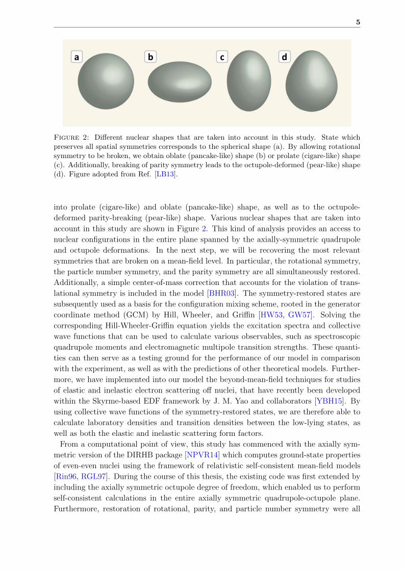
Figure 2: Different nuclear shapes that are taken into account in this study. State whichpreserves all spatial symmetries corresponds to the spherical shape (a). By allowing rotationalsymmetry to be broken, we obtain oblate (pancake-like) shape (b) or prolate (cigare-like) shape(c). Additionally, breaking of parity symmetry leads to the octupole-deformed (pear-like) shape(d). Figure adopted from Ref. [LB13].
into prolate (cigare-like) and oblate (pancake-like) shape, as well as to the octupole-
deformed parity-breaking (pear-like) shape. Various nuclear shapes that are taken into
account in this study are shown in Figure 2. This kind of analysis provides an access to
nuclear configurations in the entire plane spanned by the axially-symmetric quadrupole
and octupole deformations. In the next step, we will be recovering the most relevant
symmetries that are broken on a mean-field level. In particular, the rotational symmetry,
the particle number symmetry, and the parity symmetry are all simultaneously restored.
Additionally, a simple center-of-mass correction that accounts for the violation of trans-
lational symmetry is included in the model [BHR03]. The symmetry-restored states are
subsequently used as a basis for the configuration mixing scheme, rooted in the generator
coordinate method (GCM) by Hill, Wheeler, and Griffin [HW53, GW57]. Solving the
corresponding Hill-Wheeler-Griffin equation yields the excitation spectra and collective
wave functions that can be used to calculate various observables, such as spectroscopic
quadrupole moments and electromagnetic multipole transition strengths. These quanti-
ties can then serve as a testing ground for the performance of our model in comparison
with the experiment, as well as with the predictions of other theoretical models. Further-
more, we have implemented into our model the beyond-mean-field techniques for studies
of elastic and inelastic electron scattering off nuclei, that have recently been developed
within the Skyrme-based EDF framework by J. M. Yao and collaborators [YBH15]. By
using collective wave functions of the symmetry-restored states, we are therefore able to
calculate laboratory densities and transition densities between the low-lying states, as
well as both the elastic and inelastic scattering form factors.
From a computational point of view, this study has commenced with the axially sym-
metric version of the DIRHB package [NPVR14] which computes ground-state properties
of even-even nuclei using the framework of relativistic self-consistent mean-field models
[Rin96, RGL97]. During the course of this thesis, the existing code was first extended by
including the axially symmetric octupole degree of freedom, which enabled us to perform
self-consistent calculations in the entire axially symmetric quadrupole-octupole plane.
Furthermore, restoration of rotational, parity, and particle number symmetry were all
6
added, as well as mixing of these configurations within the GCM framework. Since the
obtained code was significantly time-consuming, it was parallelized with the OpenMP
techniques in order to make it computationally feasible. Finally, a recently developed
method for studies of electron scattering off nuclei was implemented in the model. This
provided us with the state-of-the-art tool for nuclear structure studies that can, together
with the eventual extensions, be applied in analyses of various phenomena over the entire
nuclide chart, particularly in the heavy-mass region where the framework of EDFs still
remains unrivalled among theoretical nuclear models.
In this thesis, particularly, the developed model will be applied in a study of cluster-
ing phenomena in light atomic nuclei. As the first application of the model, we chose
to focus our attention on a structure of neon and carbon isotopes. Generally speaking,
light systems are arguably the most demanding test for nuclear EDF models, not least
because few-body systems are marked by a gradual breaking of the mean-field picture and
by increasing necessity of the exact restoration of translational symmetry. On the other
hand, one of the main advantages of using the EDF framework in studies of clusters is its
feature that no localized structures are a priori assumed within the model. In fact, the
framework incorporates both the quantum-liquid and cluster aspects of nuclear systems
on the same footing, and clusterization may eventually appear only as a consequence of
the self-consistent procedure on a mean-field level and/or the subsequent configuration
mixing. In addition, parameters of the effective interaction were fitted to data on very
heavy nuclei, and therefore the interaction itself does not bear any information whatso-
ever about the light systems that we aim to tackle. Of course, globality of the approach
does not come without a price, and the employed interaction may not be able to describe
all particularities determined by shell evolution in specific mass regions. Nevertheless, in
spite of the mentioned drawbacks, it is the underlying credo of this manuscript that the
employment of such a global framework, even at (or, in some sense, especially at) the
verge of its applicability, represents a meaningful endeavor and a valuable contribution
to the lively field of nuclear cluster physics. It is left to the reader to decide for himself
on the validity of this assumption.
This manuscript is organized as follows. Part I contains detailed description of the
employed theoretical framework. In Chapter 1, we will describe the single-reference im-
plementation of relativistic EDF theory. The RHB model, a particular realization of the
theory that encompasses both mean-field and pairing correlations, will be introduced,
and effective interactions in both the particle-hole and particle-particle channels will be
discussed. Additionally, we will summarize recent results obtained by the Bruyeres-Orsay-
Zagreb collaboration on the origin and phenomenology of nuclear clustering within the
relativistic mean-field framework. In Chapter 2, the multi-reference implementation of
EDF theory will be laid out, encompassing a procedure of symmetry restoration and
configuration mixing. Furthermore, relations most pertinent for calculation of correlated
densities and form factors will be displayed. Part II contains first results obtained within
the described framework. We will start with an introductory Chapter 3 in which we will
address computational aspects of a study. In Chapter 4, a comprehensive analysis of
quadrupole-octupole collectivity and cluster structures in neon isotopes will be carried
out. Special attention will be paid to the case of the self-conjugate 20Ne isotope, where
cluster structures are thought to form already in the ground state. In Chapter 5, the

7
framework will be applied in a description of low-lying structure of 12C isotope, focusing
particularly on a structure of the Kπ = 0+ bands that are known to manifest a rich
variety of shapes. Finally, a concluding chapter will briefly summarize the results of the
present study and suggest possible extensions and improvements to the model.


Part I
Theoretical Framework
9


Chapter 1
The Nuclear Energy Density
Functional Method
Use the Force1, Luke.
Jedi Master Obi-Wan Kenobi, ”Star Wars Ep. IV”
The nuclear energy density functional (EDF) method currently provides the most com-
plete and accurate description of ground-state and excited-state properties of atomic
nuclei over the entire nuclide chart [BHR03, NVR11, RRR18]. Among microscopic ap-
proaches to the nuclear many-body problem, it is arguably the one which maintains an
optimal compromise between global accuracy and feasibility of computational cost. It is
very similar2 in form to the density functional theory (DFT) [HK64, KS65, Koh99], a
method which is widely used in condensed matter physics and quantum chemistry. In
resemblance to DFT framework, nuclear EDF models effectively map the many-body
problem onto a one-body problem by introducing relatively simple functionals of powers
and gradients of ground-state nucleon densities and currents, representing distributions of
matter, spin, momentum, and kinetic energy. In this way, a complex system of strongly-
interacting particles is substituted by a much simpler and more intuitive system of in-
dependent particles that move in a self-consistent mean-field generated by all the other
particles. On the other hand, and in contrast to the situation encountered in electronic
many-body systems, derivation of highly accurate functionals from first principles is yet
1If you are already wondering which one, this is the right chapter for you.2The main conceptual difference between EDF and DFT lies in their relation to symmetry breaking.
While EDF method minimizes energy of the system with respect to the symmetry-breaking trial wavefunction, DFT is built on an energy functional that is to be minimized with respect to a density whichpossesses all symmetries of the actual ground-state density [Dug14]. Even though, more recently, DFTframework has been extended to account for breaking of translation symmetry [Eng07], more involvedsymmetries (such as rotational or particle number) are yet to be included to the framework. The relationbetween DFT and nuclear EDF method still remains under debate [Dug14, Men16, Nak12, LDB09].
11

12 Chapter 1 The Nuclear Energy Density Functional Method
to be achieved in nuclear systems. Meanwhile, a hybrid approach is routinely employed:
(i) form of the EDF is motivated by the underlying fundamental theory and relevant
symmetries of the nucleon-nucleon force are respected, but (ii) additional free parameters
are introduced to a model. Modern functionals are typically determined by about ten to
twelve such parameters that are adjusted to a nuclear matter equation of state and to
ground-state properties of finite nuclei. The most popular phenomenological functionals
can be broadly divided into three separate classes:
• Non-relativistic Skyrme interaction. Originally introduced by T. H. R. Skyrme in
the late 50s [Sky56, Sky58] as a combination of momentum-dependent two-body
contact forces and momentum-independent three-body contact force, Skyrme func-
tionals are probably the most widely used effective interaction in studies of low-
energy nuclear structure up to date. This interaction is zero-range and quasilocal,
which makes it particularly attractive from a computational point of view. On the
other hand, pairing term is not included in the central part of an interaction and it
is therefore typically added by hand. A general overview of Skyrme formalism can
be found in Ref. [BHR03] and references cited therein.
• Non-relativistic Gogny interaction. In the late 60s, D. M. Brink and E. Boeker
introduced a finite-range nuclear interaction [BB67]. A bit over a decade later, J.
Decharge and D. Gogny proposed a new parameterization of nuclear interaction
[DG80] that became known as the Gogny force. Since within Gogny’s framework
mean-field and pairing terms have a common origin, this force is marked by a con-
sistent treatment of all parts of the interaction. Finite range of the force guarantees
a proper cut-off in momentum space, but the resulting pairing field is non-local
which can render numerical implementations rather time-consuming. Over the past
decades, various parameterizations of the force have been successfully applied in
numerous nuclear structure studies. A general overview of Gogny formalism can be
found in Refs. [Egi16, RRR18] and references cited therein.
• Relativistic interactions. Building upon a pioneering work of B. D. Serot and J. D.
Walecka from the mid-80s [SW86], manifestly covariant approaches to the nuclear
many-body problem have been developed [VALR05, NVR11, Men16]. Starting from
a field theoretical Lagrangian that obeys Lorentz symmetries, these models have
been able to match the performance of conventional non-relativistic models, while
naturally accounting for purely relativistic effects such as the spin-orbit potential or
the pseudospin symmetry [Gin97, MSTY+98]. Even though the relativistic Hartree-
Fock-Bogoliubov model has been introduced quite recently [LRGM10, EKAV11], the
vast majority of relativistic models is explicitly built as Hartree theories. In other
words, the exchange terms of nuclear interaction are usually not taken into account
explicitly and their effect is implicitly included through the free parameters of the
model. Finally, non-relativistic pairing force is typically added to the functional.
All of the listed formulations have their own advantages and drawbacks, and the choice
of interaction in each study often comes down to a particular problem in question and/or

1.1 Relativistic Mean-Field Theory 13
to a personal taste and formational tradition of a researcher. Due to a nature of the
problem in question, as well as the personal taste and formational tradition of the au-
thor of these lines3, the present study will be carried out within the relativistic frame-
work. This means that a discussion of the non-relativistic framework will be completely
omitted from the manuscript. For more information on recent applications of the non-
relativistic framework an interested reader is referred to the review papers on the Skyrme
[BHR03] and the Gogny [Egi16, RRR18] techniques. We will start this chapter with a
brief overview of the relativistic mean-field (RMF) theory. It goes almost without saying
that an intention or a capacity of this manuscript is not to give a comprehensive the-
oretical account of the framework. Much more detailed discussions can be found in a
recently published book on relativistic EDFs [Men16] and in various review articles on
the subject [Rin96, VALR05, NVR11]. For the purposes of this thesis, in Section 1.1 we
will first lay out the basic building blocks of the RMF theory, introducing the meson-
exchange and point-coupling pictures of a covariant framework. We will then proceed
to describe particular effective interactions that will be used in the particle-hole (ph)
and particle-particle (pp) channels throughout the study, that is, the density-dependent
point-coupling DD-PC1 functional and a non-relativistic force separable in the momen-
tum space, respectively. Relativistic Hartree-Bogoliubov model, which enables a unified
description of ph and pp correlations on a mean-field level, will be discussed in Section
1.2. In Section 1.3, we will summarize recent results on the origin and phenomenology of
nuclear clustering within the RMF framework that are relevant for the present work.
1.1. Relativistic Mean-Field Theory
1.1.1 Basic Building Blocks of the RMF Theory
Relativistic mean-field theory is a phenomenological, Lorentz-invariant approach to the
nuclear many-body problem. It is based on a picture of atomic nucleus as a relativistic
system of nucleons that are coupled to exchange mesons and photons through an effective
Lagrangian. Basic assumptions of the theory are [Rin96, Men16]:
• RMF is a semi-classical field theory and the effective mesons serve only to introduce
classical fields that carry appropriate relativistic quantum numbers. Consequently,
rather than being treated as dynamical degrees of freedom, the meson-field operators
are replaced by their expectation values in the nuclear ground state. More formally,
effective mesons can be thought of as collective bosonic degrees of freedom that
parameterize the non-vanishing bilinear combinations of local nucleon fields in the
Hubbard-Stratonovich sense [Hub59].
• Nucleons are treated as point-like particles and their complex substructure includ-
ing quarks and gluons is not explicitly taken into account. This approximation is
3And his respective doctoral advisors as well.

14 Chapter 1 The Nuclear Energy Density Functional Method
justified by considerations rooted in the effective field theory (EFT), since in the
low-energy regime characteristic for nuclear structure the detailed substructure of
nucleons cannot be resolved. Therefore, the explicit contribution from quarks and
gluons can be integrated out, while their effect is being completely accounted for
through the free parameters of effective Lagrangian.
• Vacuum polarization is not taken into account explicitly, that is, contributions from
the Dirac sea are neglected (the so called no-sea approximation). However, effects of
vacuum polarization are taken into account implicitly, through a phenomenological
adjustment of free parameters of a model.
• In order to correct for too large incompressibility and properly describe the nu-
clear surface properties, a density-dependence of the interaction is introduced. This
feature is not specific to relativistic interactions only, since a large majority of pa-
rameterizations of both Skyrme and Gogny interactions includes density-dependent
terms as well.
Starting point of RMF calculations is a Lagrangian density that includes coupling of
nucleons on effective mesons and photons, as well as the meson self-coupling. The attrac-
tive part of effective interaction is mediated by the exchange of scalar mesons. In fact, the
spin-zero positive-parity σ-meson, which provides the mid- and long-range attractive part
of nuclear interaction, can be understood as an approximation to the two-pion exchange
in the mesonic picture [Rin96]. The repulsive part of interaction is determined by the
exchange of vector mesons, the most important of which is the isoscalar-vector ω-meson.
Finally, isospin dependence of the nuclear force is accounted for through the exchange
of isovector-vector ρ-meson. The isoscalar-scalar σ-meson, the isoscalar-vector ω-meson,
and the isovector-vector ρ-meson build a minimal set of meson fields that is, together with
the electromagnetic field, necessary for a description of bulk and single-particle nuclear
properties [NVR11]. In principle, one could also introduce to a model the isovector-
scalar δ-meson, which would lead to a minor difference of scalar nuclear potentials in two
isospin channels. However, it was demonstrated that the effect of inclusion of δ-meson
can be completely absorbed in the readjusted coupling constant of ρ-meson [RMVC+11].
Therefore, δ-meson is omitted from majority of successful parameterizations. One should
bear in mind that RMF is a phenomenological theory and that properties of the effective
mesons do not necessarily have to coincide with properties of actual mesons known from
the experiment.
In order to take into account the higher-order many-body effects, which are needed for
a quantitative description of nuclear matter and finite nuclei, it is necessary to include
a medium dependence of the effective interaction. This can be done either by introduc-
ing non-linear meson self-couplings or by allowing for the explicit density-dependence
of the meson-nucleon couplings. Both the former [LKR97, LMGZ04, TRP05] and the
latter [HKL01, NVFR02, LNVR05] approach have so far been employed in building suc-
cessful phenomenological interactions. In the next step, the very exchange of effective
mesons in each channel (scalar-isoscalar, vector-isoscalar, scalar-isovector, and vector-
isovector) can be replaced by the corresponding local four-point (contact) interactions
1.1 Relativistic Mean-Field Theory 15
between nucleons. The main motivation for this step is a fact that the exchange of heavy
mesons is associated with short-distance dynamics which is unresolvable at low ener-
gies that are characteristic for nuclear systems. The main practical advantage, on the
other hand, is reducing the computational cost considerably by rendering the interac-
tion zero-range. It has been argued that other advantages of the point-coupling picture
include a possibility of studying the role of naturalness in effective theories for nuclear
structure-related problems [FS00], an easier inclusion of the Fock term, as well as the
transition to a framework which is more convenient to investigate relationship between
relativistic and non-relativistic models. Within the point-coupling picture, finite range
effects of the nuclear force are typically taken into account by local derivative terms,
similar to the situation encountered within the Skyrme framework. On the other hand,
medium dependence is accounted for either through density-dependent coupling constants
in two-body interactions or by including many-body contact terms. Over the past two
decades, point-coupling functionals [BMMR02, NVR08, ZLYM10] have been developed
whose performance matches that of the meson-exchange functionals. Throughout this
study we will used the density-dependent point-coupling (DD-PC1) functional [NVR08]
that was formulated in 2008 and employed in numerous studies ever since.
1.1.2 The DD-PC1 Effective Interaction
Basic building blocks of the point-coupling functional are densities and currents bilinear
in the Dirac spinor field ψ of a nucleon:
ψOτΓψ, Oτ ∈ 1, ~τ, Γ ∈ 1, γµ, γ5, γ5γµ, σµν, (1.1)
where ~τ represents Pauli isospin matrices and Γ denotes 4×4 Dirac matrices. An effective
Lagrangian is then built by forming the four-fermion (contact) combinations that behave
like scalars under Lorentz transformations and under rotations in isospin space. Possible
combinations in various isospace-space channels read:
(i) isoscalar-scalar: (ψψ)(ψψ),
(ii) isoscalar-vector: (ψγµψ)(ψγµψ),
(iii) isovector-scalar: (ψ~τψ) · (ψ~τψ),
(iv) isovector-vector: (ψ~τγµψ) · (ψ~τγµψ).
Vectors in isospin space are denoted with arrows, and vectors in coordinate space will be
marked in bold throughout the manuscript. In principle, a general effective Lagrangian
can be written as a power series of these terms and their derivatives, with higher-order
terms representing in-medium many-body correlations. However, the currently available
empirical data constrains only a limited set of parameters in such general expansion.

16 Chapter 1 The Nuclear Energy Density Functional Method
Therefore, an alternative approach is usually employed where the effective Langragian
includes only second-order interaction terms, while all of the many-body correlations are
built into a density-dependence of coupling constants. Total effective Lagrangian density
of DD-PC1 interaction reads:
LDD-PC1 = Lfree + L4f + Lder + LEM. (1.2)
Here, the first term corresponds to a Lagrangian density of free nucleons:
Lfree = ψ(iγµ∂µ −m)ψ, (1.3)
while the four-fermion point-coupling part reads:
L4f = −1
2αS(ρ)(ψψ)(ψψ)− 1
2αV (ρ)(ψγµψ)(ψγµψ)− 1
2αTV (ρ)(ψ~τγµψ)(ψ~τγµψ). (1.4)
In full analogy with the meson-exchange picture, contact part of the interaction includes
the isoscalar-scalar, isoscalar-vector and isovector-vector terms, while the isovector-scalar
term is not included into a Lagrangian. Furthermore, the derivative part includes only
the isoscalar-scalar contribution:
Lder = −1
2δS(∂νψψ)(∂νψψ). (1.5)
Even though such terms could in principle be included in each isospace-space channel,
experimental data can in practice constrain only one such term [NVR08]. Inclusion of
derivative term in the isoscalar-scalar channel only is consistent with conventional meson-
exchange RMF models, where a mass of σ-meson is adjusted to experimental data and free
values are used for masses of ω- and ρ-mesons [NVR11]. Finally, the effective Lagrangian
includes coupling of protons on electromagnetic field:
LEM = −eψAµγµ1− τ3
2ψ. (1.6)
Dynamics of a nuclear system is determined by the principle of least action:
S =
∫dx4L(x), δS = 0, (1.7)
which leads to the Euler-Lagrange equation:

1.1 Relativistic Mean-Field Theory 17
∂L∂ψ
+∂L∂ρV
∂ρV∂ψ− ∂µ
∂L∂(∂µψ)
= 0. (1.8)
Carrying out variation of Lagrangian with respect to the adjoint spinor ψ yields the
single-nucleon Dirac equation:
[γµ
(i∂µ − Σµ
V − ΣµTV − Σµ
R
)−(m+ ΣS
)]ψ = 0, (1.9)
where the isoscalar-scalar nucleon self-energy ΣS, the isoscalar-vector self-energy ΣµV , and
the isovector-vector self-energy ΣµTV read:
ΣS = αS(ρV )(ψψ)− δS∆(ψψ), (1.10)
ΣµV = αV (ρV )(ψγµψ) + e
1− τ3
2Aµ, (1.11)
ΣµTV = αTV (ρV )(ψ~τγµψ). (1.12)
In addition, Dirac equations includes contribution from the rearrangement term:
ΣµR =
1
2
ψγµψ
ρV
[dαSdρV
(ψψ)(ψψ) +dαVdρV
(ψγµψ)(ψγµψ) +dαTVdρV
(ψ~τγµψ)(ψ~τγµψ)], (1.13)
which arises from variation of density-dependent coupling constants αS, αV , and αTV with
respect to nucleon field ψ. For models with density-dependent couplings, inclusion of the
rearrangement self-energies is shown to be essential for energy-momentum conservation
and thermodynamic consistency [NVFR02, FLW95]. In addition, it is assumed that
couplings are functions of vector density, ρV =√jµjµ, where jµ = ψγµψ is the nucleon
four-current. Alternative option would have been making the couplings functions of
scalar density. Nevertheless, vector density appears as a more natural choice because it
is related to a conserved nucleon number, while no such conservation law holds in a case
of scalar density. Guided by the microscopic density dependence of the vector and scalar
self-energies in nuclear matter, a particular ansatz for the functional form of couplings is
introduced [NVR08]:
αi(ρV ) = ai + (bi + cix)e−dix, (i = S, V, TV ), (1.14)
where x = ρV /ρsat, ρsat = 0.152 fm−3 denotes nucleon saturation density in symmetric
nuclear matter, and twelve free parameters are yet to be determined via fitting procedure.
Dirac equation (1.9) describes dynamics of a nuclear system. On the other hand,
the corresponding EDF can be derived by employing the Legendre transformation on a

18 Chapter 1 The Nuclear Energy Density Functional Method
Table 1.1: List of phenomenological parameters of DD-PC1 functional (first row) and theiradopted values obtained by fitting to experimental data on infinite nuclear matter and finitenuclei (second row) [NVR08]. See text for details.
aS [fm2] bS [fm2] cS [fm2] dS aV [fm2] bV [fm2] dV bTV [fm2] dTV δS [fm4]
−10.0462 −9.1504 −6.4273 1.3724 5.9195 8.8637 0.6584 1.8360 0.6400 −0.8150
Lagrangian density L. This yields the Hamiltonian density H:
H =∂L
∂(∂0φi)∂0φi − L, (1.15)
where φi represents either nucleon or photon field. Hamiltonian density, which corre-
sponds to the 00 component of energy-momentum tensor, is then used to determine the
effective Hamiltonian operator H4:
H =
∫d3rH(r). (1.16)
Within the mean-field approximation, the total correlated many-body state |Ψ〉 is repre-
sented by a simple product state |Φ〉. The DD-PC1 energy density functional corresponds
to the expectation value of the effective Hamiltonian operator in this product state:
EDD-PC1[ρ] ≡ 〈Φ|H|Φ〉 =
∫d3rE(r), (1.17)
where a total energy density:
E(r) = Ekin(r) + E int(r) + EEM(r) (1.18)
is composed of the kinetic part Ekin(r), the interaction part E int(r), and the electromag-
netic part EEM(r):
Ekin(r) =N∑i=1
ψ†αi(ααα · p + βm
)ψαi , (1.19)
E int(r) =1
2αSρ
2S +
1
2αV jµj
µ +1
2αTV~jµ~j
µ +1
2δSρS∆ρS, (1.20)
EEM(r) =1
2ejµcAµ. (1.21)
4We call our Hamiltonian operator effective because it explicitly depends on nucleonic density and assuch it is different from a genuine density-independent Hamiltonian operator. This distinction lies at theroot of some theoretical difficulties that can manifest themselves on a multi-reference level and that willbe discussed in the next chapter.

1.1 Relativistic Mean-Field Theory 19
Here, we have introduced a shorthand notation for the scalar density ρS, the baryon
current jµ = (ρV , j), the isovector current ~jµ = (ρ3, j3), and the electromagnetic current
jµc = (ρc, jc) in the self-consistent ground state of atomic nucleus:
ρS(r) ≡ 〈Φ|ψψ|Φ〉 =N∑i=1
ψαi(r)ψαi(r), (1.22a)
jµ(r) ≡ 〈Φ|ψγµψ|Φ〉 =N∑i=1
ψαi(r)γµψαi(r), (1.22b)
~jµ(r) ≡ 〈Φ|ψ~τγµψ|Φ〉 =N∑i=1
ψαi(r)~τγµψαi(r), (1.22c)
jµc (r) ≡ 〈Φ|ψγµ1− τ3
2ψ|Φ〉 =
N∑i=1
ψαi(r)γµ1− τ3
2ψαi(r), (1.22d)
where sums run over all occupied positive-energy single-nucleon orbitals. Particular struc-
ture of |Φ〉 will be discussed in Section 1.2. The ground-state energy of a nuclear system
(1.17) is determined by a self-consistent solution to the Dirac equation (1.9). Starting
from an initial nuclear field (usually something of the Woods-Saxon type), a first set of
orbitals ψi can be obtained. These orbitals are then used to calculate densities and
currents, (1.22a) - (1.22d), which give rise to refined nuclear fields, (1.10) - (1.13). In the
next step, these fields serve as a new source to the Dirac equation. The self-consistent
procedure is repeated until a convergence is reached and a ground-state description of
atomic nucleus is obtained.
Twelve parameters in various isospace-space channels together with the strength pa-
rameter of a derivative term form an initial set of 13 free parameters of the DD-PC1
interaction. Some of them will be discarded prior to the fitting procedure. To start with,
a functional form of coupling constant in the isovector-vector channel was determined
from results of Dirac-Brueckner calculations of asymmetric nuclear matter [dJL98], and
two parameters (aTV and cTV ) were therefore set to zero [NVR08]. In addition, param-
eter cV was also set to zero in order to reduce a number of parameters. The remaining
ten parameters were simultaneously adjusted to infinite and semi-infinite nuclear matter
properties, as well as to the binding energies of 64 axially symmetric deformed nuclei in
mass regions A ≈ 150 − 180 and A ≈ 230 − 250. Details of the fitting procedure can
be found in Ref. [NVR08], while in Table 1.1 we list the adopted values of parameters5.
DD-PC1 functional has been further tested in calculations of ground-state properties
of spherical and deformed medium-heavy and heavy nuclei, including binding energies,
charge radii, deformation parameters, neutron skin thickness, and excitation energies of
giant multipole resonance. The only relevant deviations from data have been found in
calculations of binding energies in spherical closed-shell nuclei. This discrepancy can be
understood in terms of a relatively low effective nucleon mass that, when a relativistic
5It is interesting to mention that, quite recently, concepts from information geometry were used toanalyze parameter sensitivity for a nuclear energy density functional, improve the fitting procedure, andeventually further reduce a number of parameters [NV16, NIV17].

20 Chapter 1 The Nuclear Energy Density Functional Method
(a) (b)
Figure 1.1: Performance of DD-PC1 functional with two different beyond mean-field models.Left panel (a): Low-lying spectra of 226Th calculated with DD-PC1 functional within the IBMframework in comparison with experimental data [NVNL14]. Right panel (b): Low-lying spectraof 76Ge calculated with DD-PC1 functional and collective Hamiltonian model in comparison withexperimental data [NMV14].
functional is adjusted to binding energies of deformed nuclei, yields overbinding in spheri-
cal systems. Save for these disagreements in a vicinity of closed shells, a very good overall
agreement with data has been obtained (see Sec. IV of Ref. [NVR08]). Furthermore, per-
formance of the DD-PC1 functional was additionally tested in subsequent studies within
different beyond mean-field models [NVNL14, NMV14]. In Ref. [NVNL14], the inter-
acting boson model (IBM) Hamiltonian was built from energy surfaces generated with
constrained calculations based on the DD-PC1 functional. This Hamiltonian was further
employed in calculations of energy spectra and transition rates in different medium-heavy
and heavy isotopes. In the left panel of Figure 1.1, we show calculated spectroscopy of226Th isotope in comparison with available data. In Ref. [NMV14], the shape coexistence
and triaxiality in germanium isotopes were studied within the framework of collective
Hamiltonian based on DD-PC1 functional. The right panel of Fig. 1.1 displays obtained
low-energy structure of 76Ge isotope in comparison with available data. Both mean-field
and beyond mean-field applications of DD-PC1 functional arguably place it among the
most successful contemporary functionals and justify the choice of an effective interaction
for the present study.
1.1.3 The Separable Pairing Force
EDF method, in a form described in previous subsection, can account for only a very
small number of doubly magic nuclei. Moving further away from closed shells, however,
the inclusion of correlations related to pairing of two nucleons (particle-particle correla-
tions) becomes crucial for a quantitative description of many nuclear structure phenom-
ena. In principle, particle-particle interaction is isospin-dependent and both T = 1 and
T = 0 components of the interaction should be taken into account. For a large majority
of nuclei, dominant contribution to pairing phenomenon stems from a correlated state of
like-particles (two protons or two neutrons) that are coupled to total angular momentum
1.1 Relativistic Mean-Field Theory 21
zero and total isospin one. On the other hand, when a number of neutrons approaches a
number of protons, two types of nucleons occupy similar orbitals near Fermi surface and
neutron-proton pairs can be formed in both the T = 1 and T = 0 channel [FM14]. How-
ever, due to the breaking of the underlying signature symmetry, simultaneous inclusion
of both types of pairing is notoriously complicated within the EDF framework [BHR03].
Therefore, in this work we adopt a strategy of virtually all EDF models and explicitly
treat only the like-particle pairing. Furthermore, even though relativistic pairing interac-
tions in finite nuclei have been formally developed, at the moment there is no empirical
evidence for any relativistic effects in nucleon pairing [Ser01]. Therefore, in this work we
employ a standard hybrid method by adding the non-relativistic pairing force to the rela-
tivistic energy density functional (more details on this method can be found, for example,
in a review paper of Ref. [VALR05]). Commonly used tactics in relativistic models is
including a pairing force which is based on the Gogny interaction. On the one hand, this
choice avoids a problem of cutoff dependence which plagues zero-range implementations
of pairing force, such as monopole pairing or density-dependent δ-pairing interactions.
On the other hand, a price to pay is the non-locality of pairing field and, consequently,
the inherited complexity of numerical implementation. In order to reduce the cost of nu-
merical implementation, a separable form of pairing has been introduced in calculations
of both spherical and deformed nuclei [Dug04, TMR09c, TMR09a, TMR09b, NRV+10].
Simple separable forces are demonstrated to reproduce pairing properties in spherical and
deformed nuclei on almost the same footing as the original Gogny force, while reducing a
computational cost significantly. As additional features, they both preserve translational
invariance and maintain a finite range.
The separable pairing force that will be used throughout this study is a non-relativistic
force separable in momentum space [TMR09a, TMR09b]:
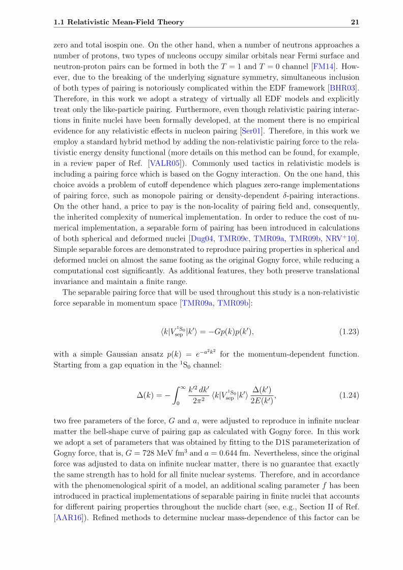
〈k|V 1S0sep |k′〉 = −Gp(k)p(k′), (1.23)
with a simple Gaussian ansatz p(k) = e−a2k2 for the momentum-dependent function.
Starting from a gap equation in the 1S0 channel:
∆(k) = −∫ ∞
0
k′2 dk′
2π2〈k|V 1S0
sep |k′〉∆(k′)
2E(k′), (1.24)
two free parameters of the force, G and a, were adjusted to reproduce in infinite nuclear
matter the bell-shape curve of pairing gap as calculated with Gogny force. In this work
we adopt a set of parameters that was obtained by fitting to the D1S parameterization of
Gogny force, that is, G = 728 MeV fm3 and a = 0.644 fm. Nevertheless, since the original
force was adjusted to data on infinite nuclear matter, there is no guarantee that exactly
the same strength has to hold for all finite nuclear systems. Therefore, and in accordance
with the phenomenological spirit of a model, an additional scaling parameter f has been
introduced in practical implementations of separable pairing in finite nuclei that accounts
for different pairing properties throughout the nuclide chart (see, e.g., Section II of Ref.
[AAR16]). Refined methods to determine nuclear mass-dependence of this factor can be

22 Chapter 1 The Nuclear Energy Density Functional Method
employed, such as fine tuning it in a comparison between experimental moments of inertia
and those obtained in cranked relativistic Hartree-Bogoliubov calculations [AARR14,
AAR16]. In this work, however, we choose to simply fix the value of scaling parameter
to f = 0.9 and use the same pairing force throughout the entire study.
In order to determine matrix elements of the paring interaction, a separable force of
Eq. (1.23) is first transformed from momentum space to coordinate space:
V (r1, r2, r′1, r′2) = −Gδ(R−R′)P (r)P (r′)
1
2(1− Pσ), (1.25)
where R = 12(r1 + r2) and r = r1− r2 denote the center of mass and relative coordinates
of two paired particles, respectively, and Pσ = σ1 ·σ2 is a spin operator. In addition, P (r)
corresponds to a Fourier transform of p(k) and reads:
P (r) =1
(4πa2)3/2e−
z2+r2⊥4a2 . (1.26)
Obviously, separable pairing force has a finite range in coordinate space. In addition,
because of the presence of δ(R−R′), it preserves a translational invariance. To proceed
further with our calculation, it is necessary to define a relevant single-particle basis in
which the pairing force matrix elements will be computed. Prior to that, let us first
introduce a framework that provides a unified self-consistent account of both mean-field
and pairing correlations.
1.2. Relativistic Hartree-Bogoliubov Model
1.2.1 The Independent Quasiparticle Picture
So far, we have defined and discussed effective interactions in two distinct interaction
channels, that is, the density-dependent point-coupling (DD-PC1) functional in particle-
hole channel and the separable pairing force in particle-particle channel. In this section,
we will introduce a framework which enables us to treat two of those simultaneously and
on an equal footing (detailed discussions on this framework can be found in standard
textbooks [RS80, BR85] and references cited therein). In order to achieve that, we will
first have to give up on the intuitive picture of independent particles (nucleons), that are
associated with a set of single-particle operators c†α, cα and can be generated from a
physical vacuum |0〉 via |α〉 = c†α |0〉6. Since pairing correlations scatter pairs of nucle-
ons in time-reversed states around the Fermi surface, single nucleons do not represent
convenient degrees of freedom anymore. In place of that, one introduces a concept of
independent quasiparticles, that can be thought of as independent particles dressed in
correlations generated by pairing interaction. These quasiparticles are associated with a
6More details on the second quantization formalism are given in Appendix A.

1.2 Relativistic Hartree-Bogoliubov Model 23
set of single-quasiparticle operators ↵, βµ, and a transition between particle and quasi-
particle frameworks is given by the unitary Bogoliubov transformation [RS80, BR85]:
βµ =∑α
(U∗αµcα + V ∗αµc
†α
), (1.27)
↵ =∑α
(Uαµc
†α + Vαµcα
), (1.28)
where sums run over the entire configuration space. Evidently, quasiparticle operators
mix particle creation and annihilation operators. Nevertheless, they still satisfy standard
fermionic anticommutation relations:
βµ, βν = 0, ↵, β†ν = 0, βµ, β†ν = δµν . (1.29)
Bogoliubov transformation can be written in a more compact form:
(β
β†
)=W†
(c
c†
), (1.30)
where the unitary transformational matrix W reads:
W =
(U V ∗
V ∗ U
). (1.31)
Bogoliubov matrices U and V play a central role within this framework, as they determine
properties of independent quasiparticles. However, their form is not completely arbitrary.
In fact, as a consequence of anticommutation relations for quasiparticle operators (1.29),
it can be shown that Bogoliubov matrices need to satisfy the following expressions:
U †U + V †V = 1, UU † + V ∗V T = 1,
UTV + V TU = 0, UV † + V ∗UT = 0.(1.32)
Within the non-relativistic quasiparticle picture, ground state of the nuclear many-body
system |Φ〉 is constructed by applying quasiparticle annihilation operators on a true (bare)
vacuum state:
|Φ〉 =∏µ
βµ |0〉 . (1.33)

24 Chapter 1 The Nuclear Energy Density Functional Method
This, in turn, means that the ground state is now a vacuum with respect to independent
quasiparticles:
βµ |Φ〉 = 0, ∀µ. (1.34)
State that satisfies these conditions for a corresponding set of quasiparticle operators
↵, ⵠis called the Hartree-Fock-Bogoliubov (HFB) state. In the next subsection, we
will discuss a particular realization of HFB theory, the relativistic Hartree-Bogoliubov
(RHB) model.
1.2.2 Relativistic Hartree-Bogoliubov Equation
The HFB framework, as already emphasized several times throughout this manuscript,
provides a unified description of ph and pp correlations on a mean-field level. In con-
trast to more phenomenological approaches such as the Bardeen-Cooper-Schrieffer (BCS)
theory, HFB model is applicable across the entire chart of nuclides, for strongly-bound
and weakly-bound nuclei alike. We point out that a particular realization of HFB theory
which will be used in this work, the relativistic Hartree-Bogoliubov model, bears some
differences in comparison to the conventional HFB framework [Val61]. Here, we list some
of the most relevant ones:
• Formally speaking, HFB framework is developed within the Hamiltonian-based pic-
ture, meaning that a starting point of the conventional HFB calculation is a genuine
Hamiltonian operator. On the other hand, starting point of our calculation is a phe-
nomenological EDF of normal and anomalous densities.
• Unlike the situation encountered in the original HFB framework, mean-field and
pairing part of our interaction are derived from different sources.
• Fock (exchange) terms are excluded from our calculation, in both the mean-field
and pairing channels of interaction.
• Due to a covariant structure of framework, relativistic Bogoliubov matrices U and
V will additionally differentiate between large and small components of nucleonic
wave function, a feature which is absent from the non-relativistic formulations of
the theory.
The RHB model defined in this way has proven to be a highly successful framework for a
relativistic description of ground state properties of atomic nuclei [Men16, NVR11]. The
RHB state |Φ〉 and single-particle operators c†α, cα can be used to define a Hermitian
normal density ρ and a skew-symmetric pairing tensor (anomalous density) κ:

1.2 Relativistic Hartree-Bogoliubov Model 25
ραγ =〈Φ|c†γcα|Φ〉〈Φ|Φ〉
=(V ∗V T
)αγ, (1.35)
καγ =〈Φ|cγcα|Φ〉〈Φ|Φ〉
=(V ∗UT
)αγ, (1.36)
κ∗αγ =〈Φ|c†αc†γ|Φ〉〈Φ|Φ〉
=(V U †
)αγ. (1.37)
Once pairing is included into the model, the EDF does not anymore depend on a normal
density only, but it additionally becomes a functional of a pairing tensor:
ERHB[ρ, κ, κ∗] = ERMF[ρ] + Epair[κ, κ∗]. (1.38)
Here, ERMF[ρ] is the usual relativistic mean-field functional, while the pairing functional
can be calculated as:
Epair[κ, κ∗] =
1
4
∑α1γ1
∑α2γ2
κ∗α1γ1〈α1γ1|V pp|α2γ2〉 κα2γ2 , (1.39)
with 〈α1γ1|V pp|α2γ2〉 representing matrix elements of a general two-body pairing interac-
tion. In the present work, a mean-field functional corresponds to the DD-PC1 functional
as defined in (1.17), while pairing matrix elements are derived from a separable pairing
force of (1.25). Normal density ρ and anomalous density κ build together the generalized
density matrix R:
R =
(ρ κ
−κ∗ 1− ρ∗
), (1.40)
which is idempotent and encodes all of the information about nuclear system that was
originally present in the RHB wave function |Φ〉. Within the Hamiltonian-based picture
of HFB, a Wick theorem with respect to |Φ〉 is employed in order to determine energy
functional E[ρ, κ, κ∗] that depends on normal and anomalous density. In the next step,
one varies:
δ[E[ρ, κ, κ∗]− λTrρ − Trλ(R2 − R)
]= 0 (1.41)
with respect to δR, which yields HFB equation. Relativistic Hartree-Bogoliubov equation
has precisely the same form and it reads:

26 Chapter 1 The Nuclear Energy Density Functional Method
(hD − λ ∆
−∆∗ −h∗D + λ
)(UkVk
)= Ek
(UkVk
). (1.42)
The left-hand side of Eq. (1.42) contains two fields. The self-consistent (Hartree-Fock)
field hD corresponds to the Dirac Hamiltonian of Eq. (1.9) and it is drives the single-
particle shell structure of atomic nucleus, while the pairing (Bogoliubov) field ∆ is respon-
sible for scattering of paired nucleons around the Fermi surface. The chemical potential
λ is determined by the particle number subsidiary condition that the expectation value
of particle number operator in nuclear ground state corresponds to the actual number
of nucleons. Column vectors of the RHB eigenvalue problem denote quasiparticle wave
functions, and Ek are quasiparticle energies. We note that a dimension of the RHB equa-
tion is twice as large as a dimension of the corresponding Dirac equation. Therefore, for
each eigenvector (Uk, Vk) with positive quasiparticle energy Ek > 0 there exists an eigen-
vector (V ∗k , U∗k ) with negative quasiparticle energy −Ek. Due to a fermionic character
of the theory, levels Ek and −Ek cannot be occupied simultaneously, that is, one needs
to choose either the positive or negative eigenvalue and the corresponding eigenvector.
Within the no sea approximation, one should in principle choose solutions with posi-
tive quasiparticle energies (particles) for states above the Dirac sea, and solutions with
negative quasiparticle energies (antiparticles) for states in the Dirac sea [Men16]. Never-
theless, due to a large Dirac gap, contribution of antiparticles to normal and anomalous
densities is negligible7. Therefore, in this work we employ a common tactics and take
into account only contributions from positive energy states. This choice enabled us to
reduce a computational time significantly by reducing a dimension of the corresponding
equation. On the other hand, a price we were willing to pay was rendering the anomalous
density κ antisymmetric only up to an excellent approximation.
Within the RHB framework, quasiparticle wave functions are composed of the large
component f and the small component g:
Uk =
(f
(U)k
ig(U)k
), Vk =
(f
(V )k
ig(V )k
). (1.43)
The corresponding equations can be solved either directly in the coordinate space [MR96,
MPR97] or, more commonly, by expanding nuclear spinors in a discrete basis of choice,
typically harmonic oscillator [GRT90] or Woods-Saxon [ZMR03] basis. In this work, we
employ a mixed method that combines the configurational and coordinate space represen-
tations [Vau73, NPVR14]. Since axial-symmetry of RHB states is imposed, corresponding
equation (1.42) is first solved in the configurational space of the axially symmetric har-
monic oscillator. In the next step, obtained wave functions are used to calculate densities
and currents in the coordinate space. Eigenfunctions of the axially symmetric harmonic
oscillator Φα(r, s) are characterized by a set of quantum numbers α = nz, n⊥,Λ,ms,where nz and n⊥ represent a number of quanta (nodes) in the z− and the r⊥− directions
7We have verified computationally that this statement indeed holds in practice.

1.2 Relativistic Hartree-Bogoliubov Model 27
of cylindrical coordinate system, respectively, while Λ and ms denote components of the
orbital angular momentum and of the spin along the z-axis. Details of the harmonic oscil-
lator basis and its coordinate representation in terms of Hermite and associated Laguerre
polynomials are given in Appendix A. Here, we note the explicit expansion of Dirac spinor
in terms of basis states Φα(r, s) and isospin wave function χti :
ψ(i)k (r, s, t) =
(∑αmaxα f
(i)α,kΦα(r, s)χti(t)
i∑αmax
α g(i)α,kΦα(r, s)χti(t)
), i = U, V. (1.44)
In order to avoid the appearance of spurious states with a very large number of radial
nodes close to the Fermi surface, maximal quantum numbers for the expansion of large
and small component of Dirac spinor, αmax and αmax, are different [GRT90]. In particular,
quantum numbers α and α are determined in such a way that the corresponding major
oscillator quantum numbers N = 2n⊥+nz + Λ are not larger than Nsh for the expansion
of large components and not larger than Nsh + 1 for the expansion of small components.
The i = V component of Dirac spinor (1.44) is used to calculate densities and currents
in the coordinate space (1.22a)-(1.22d). On the other hand, pairing tensor κ is kept in
the configurational space and the corresponding matrix elements of pairing field ∆ can
be calculated as:
∆α1γ1 =1
2
∑α2γ2
〈α1γ1|V pp|α2γ2〉 κα2γ2 . (1.45)
Here, 〈α1γ1|V pp|α2γ2〉 corresponds to a matrix element of the two-body pairing interaction
(1.25) in the harmonic oscillator basis that can be computed using the Talmi-Moshinsky
techniques for cylindrical coordinates (more details can be found in Ref. [TMR09c] and
references cited therein). In practical implementations, only large components of (1.44)
are used to build non-relativistic pairing tensor κ (1.36), while other components of the
tensor are safely omitted. By expanding nuclear spinors in a sufficiently large harmonic
oscillator basis, self-consistent solution to the RHB equation provides us with an approx-
imate description of a ground state of atomic nucleus. In spite of a fact that it formally
corresponds to a symmetry-broken wave packet of various eigenstates with good quantum
numbers (such as angular momenta, particle numbers, etc.), the RHB-type state repre-
sents a powerful tool for accessing different nuclear ground-state properties, including
binding energies, radii, and deformation parameters. Moreover, by imposing constraints
on values of different quantities, the RHB framework grants us the license to explore
energy landscapes around the self-consistent minima.
1.2.3 Constrained RHB Calculation
The conventional HFB framework, both in its spirit and its basic implementation, is
a ground-state theory. This means that, as long as employed without any additional

28 Chapter 1 The Nuclear Energy Density Functional Method
constraints, the virtue of Ritz variational principle will grant us a state that minimizes
a total energy of the system. Nevertheless, by imposing additional constraints on values
of various quantities, it is possible to obtain a state that minimizes a total energy of the
system under that very constraint. For example, by imposing a constraint on values of
nuclear radii it is possible to artificially inflate a nucleus and thereby study the role of
saturation in forming of α-clusters [GS13, EKNV14a]. Another possibility is including a
constraint on particle-number dispersion in order to study the effect of pairing fluctuations
on fission dynamics [ZLN+16]. The most common constraints, however, are those imposed
on values of electric multipole moments or, equivalently, deformation parameters. Of
course, a pool of possible constraints is primarily determined by a choice of symmetries
that nuclear system is a priori allowed or forbidden to break. In this work, we impose
the axial and time-reversal symmetry of RHB states, which means that triaxial shapes
and odd systems are out of the reach to start with. On the other hand, we allow our
even-even nucleus to deform in both the quadrupole and octupole direction. A choice
of the quadrupole degree of freedom is rather obvious, since all nuclei (except for very
few doubly-magic isotopes) exhibit deviations from a spherical shape. A choice of the
octupole degree of freedom is motivated by a fact that many α-clusterized structures, such
as the expected 16O +α configuration in 20Ne isotope, are characterized by precisely the
parity-breaking octupole deformation. In practice, we employ the method of quadratic
constraint and impose constraints on the quadrupole Q20 and octupole Q30 moments.
This method uses an unrestricted variation of the function:
〈H〉+∑λ=2,3
Cλ0
(〈Qλ0〉 − qλ0
)2, (1.46)
where 〈H〉 is total energy, 〈Qλ0〉 denotes expectation value of the mass multipole oper-
ators Qλµ ≡ rλYλµ, qλ0 are the constrained values of multipole operators, and Cλ0 are
corresponding stiffness constants. In general, values of multipole moments 〈Qλ0〉 will
coincide with constrained values qλ0 only at a stationary point, and a difference will de-
pend on stiffness constant Cλ0. In particular, smaller values of Cλ0 will lead to larger
deviations of 〈Qλ0〉 from the corresponding qλ0, while increasing Cλ0 often destroys con-
vergence of the self-consistent procedure. This deficiency can be resolved by implementing
the augmented Lagrangian method [SSBN10]. Furthermore, we introduce dimensionless
deformation parameters βλ, defined as:
βλ =4π
3ARλqλ0, R = r0A
1/3, (1.47)
with r0 = 1.2 fm. This kind of constrained calculus enables us to access configurations in
the entire plane spanned by a set of deformations q = β2, β3, and the corresponding
RHB states will be denoted as |Φ(q)〉. An interesting analysis can be carried out already
on this level, particularly in terms of the rigidness/softness of constrained energy surfaces
that determine relevance of collective correlations related to symmetry restoration and
configuration mixing. In addition, appearance of local minima on energy landscapes may

1.3 Nuclear Clustering within the RMF Framework 29
Figure 1.2: Self-consistent ground-state densities of 20Ne isotope in the x − z plane of theintrinsic reference frame. Densities calculated with the relativistic DD-ME2 functional (leftpanel) and the non-relativistic Skyrme SLy4 functional (right panel) are compared. The twoinserts on each panel show the corresponding three-dimensional density plots and the densityprofiles (ρ) along the symmetry axis (x = 0). Figure taken from Ref. [EKNV12].
offer a qualitative insight into the structure of excited nuclear configurations. Neverthe-
less, in order to carry out a more quantitative analysis, it would be beneficial to have
a framework that treats all of these configurations on an equal footing and determines
their relative contributions to a true ground state via variational procedure. A frame-
work which does precisely that exists, and it is known as the MR-EDF. It is essentially
a two-step process. In the first step, one restores relevant symmetries that are broken
on a mean-field level. For a present study, these include rotational, particle number,
and parity symmetry. In the second step, collective state of atomic nucleus is built from
symmetry-conserving configurations, and detailed description of nuclear spectroscopy is
obtained via variational procedure. The practical extension of RHB framework to a multi-
reference level represents the main original contribution of this manuscript and it will be
extensively discussed in Chapter 2. Before that, let us just briefly overview some of the
recent results on nuclear clustering that have been obtained within the RMF framework.
1.3. Nuclear Clustering within the RMF Framework
Cluster structures in α-conjugate nuclei have been a subject of numerous studies within
the mean-field framework [ASPG05, MKS+06, RMUO11, IMIO11, RB11, GS13, Rob14].
The purpose or the capacity of this section is not to give a comprehensive and balanced
overview of nuclear clustering from the mean-field perspective, or even from the relativis-
tic mean-field perspective. Rather than that, we will briefly overview some of the recent
results that have been obtained by the Bruyeres-Orsay-Zagreb collaboration and that
elucidate a context of the present work. Let us start with the self-consistent ground-state
density distributions of 20Ne isotope [EKNV12] that are plotted in Figure 1.2. Mean-field

30 Chapter 1 The Nuclear Energy Density Functional Method
Figure 1.3: Harmonic oscillator potentials with different depths. Upper panel: Three po-tentials (V0 = −30,−45,−60 MeV) with the same radius (R = 3 fm) as functions of radialcoordinate r. Lower panel: Radial wavefunctions ukl(r) of the corresponding first p-state,where k and l are the radial and the azimuthal quantum number, respectively. Figure takenfrom Ref. [EKNV12].
calculations were carried out by using representatives of two different classes of function-
als: the relativistic meson-exchange DD-ME2 functional [LNVR05] (left panel) and the
non-relativistic Skyrme SLy4 functional [CBH+98] (right panel). Both functionals repro-
duce experimental ground-state observables such as binding energies, charge, and matter
radii with a typical accuracy of roughly 1%. In addition, they yield very similar values
of equilibrium deformation parameters. Nevertheless, the obtained intrinsic densities are
manifestly different. As can be seen in Fig. 1.2, density obtained with the non-relativistic
functional exhibits smooth behavior typical of Fermi liquids, with an extended surface
region in which the density decreases very gradually from the central value of around
0.16 fm−3. The relativistic functional, on the other hand, predicts a much more localized
density, with density peaks as large as 0.20 fm−3. Different localization profiles of equi-
librium densities can be traced back to the different energy spacing of the corresponding
single-nucleon spectra [EKNV12], that are proportional to the intrinsic deformation and

1.3 Nuclear Clustering within the RMF Framework 31
Figure 1.4: Microscopic axially symmetric RHB prediction of nuclei that have small radialdispersion of the single-particle states of valence nucleons ∆r (red circles), plotted on the back-ground of empirically known nuclides in the N − Z plane. Figure taken from Ref. [EKLV18].
to the depth of the underlying single-nucleon potential. Since both functionals predict al-
most identical equilibrium deformations, differences in densities were linked to differences
in the corresponding potentials. As already noted in Ref. [EKNV14b], this situation
is rather similar to the one encountered in gaseous systems of ultracold atoms held in
three-dimensional optical lattice potentials [GME+02]. By gradually increasing the depth
of the confining potential, one can observe the transition from a phase in which each
atom is spread out over the entire lattice to the insulating phase of localized atoms. Of
course, in the self-bound systems like atomic nuclei one cannot simply vary the depth of
the single-nucleon potential, but equivalent effect is obtained by performing calculations
with different effective interactions. In fact, depth of the DD-ME2 single-neutron (single-
proton) potential for 20Ne isotope is −78.6 MeV (−72.8 MeV), and it is pronouncedly
deeper than the corresponding depths −69.5 MeV (−64.6 MeV) of the SLy4 functional.
Within the relativistic framework, depth of the single-nucleon potential is determined by
the two local self-consistent potentials of opposite signs: the attractive scalar potential
(S ≈ −400 MeV) and the repulsive vector potential (V ≈ 320 MeV). Their sum V + S
uniquely determines the confining nuclear potential, while their difference V −S simulta-
neously governs the splitting between spin-orbit partners in finite nuclei. Consequently,
the effective single-nucleon spin-orbit force for finite nuclei manifests itself naturally with
the empirical strength within the relativistic framework. On the other hand, the non-
relativistic approaches include the spin-orbit potential in a purely phenomenological way,

32 Chapter 1 The Nuclear Energy Density Functional Method
with the interaction strength that is adjusted to empirical energy spacings between the
spin-orbit partners.
The effect of depth of potential on localization of wave functions is schematically de-
picted in Figure 1.3. In the upper panel, we show three harmonic oscillator potentials
with different depths (V0 = 30, 45, and 60 MeV) but with the same radii R = 3 fm.
The lower panel shows the radial wavefunctions of the corresponding p-states. It is obvi-
ous that a larger depth of the potential leads to a smaller oscillator length and, finally,
to a more pronounced localization of the wave function in both the classically allowed
and forbidden region. On a more quantitative level, one can introduce the localization
parameter α [EKNV13, EKLV18]:
αloc ≡2∆r
r, (1.48)
which corresponds to a ratio between the spatial dispersion of the single-nucleon wave
function:
∆r =
√〈r2〉 − 〈r〉2, (1.49)
and the average internucleon distance r. For large values of α nucleons are delocalized
and nucleus behaves as a quantum liquid. For example, the doubly-magic 208Pb isotope
has self-consistent values of localization parameter roughly α ≈ 1.3, both within the
relativistic and non-relativistic framework [EKNV13], and it exhibits a typical quantum-
liquid behavior. At the opposite end, when the average internucleon distance exceeds
the nucleon spatial dispersion, nucleons localize on nodes of the hypothetical crystal-
like structure. The intermediate values of α are marked by a hybrid phase of cluster
states which are expected to appear for α ≈ 1 values. Within the harmonic oscillator
approximation, the localization parameter of Eq. (1.50) can be expressed as [EKLV18]:
αHO '√
~(2n− 1)
(2mV0r20)1/4
A1/6, (1.50)
where n corresponds to the radial quantum number, V0 denotes the depth of the potential
at r = 0, and r0 = 1.25 fm is a constant. This expression nicely elucidates the assertion
that the deeper potential favors formation of clusters, as larger V0 values explicitly yield
smaller values of the localization parameter. In addition, dependence of the localization
parameter αHO on A1/6 shows that cluster states are preferably formed in lighter nuclei,
and the transition from coexisting cluster and mean-field states to a Fermi-liquid state
should occur for nuclei with A ≈ 20 − 30 [EKNV13, EKLV18], which is in qualitative
agreement with the experiment [FHKE+18]. Of course, a more quantitative analysis re-
quires a more microscopic approach. Self-consistent ground-state solutions for a set of
self-conjugate nuclei were used to calculate corresponding α values both within the rel-
ativistic and non-relativistic framework [EKNV13]. The general conclusion was that the

1.3 Nuclear Clustering within the RMF Framework 33
Figure 1.5: Mean value of the energy gap between consecutive occupied neutron single-particlelevels as a function of axial quadrupole deformation parameter β2 in 20Ne isotope. The insetsdisplay the total nucleonic density at the corresponding deformation. In order to limit thevertical scale, the maximum mean value of the energy gap in the plot does not exceed 5 MeV.Figure taken from Ref. [EKNV14b].
values calculated with DD-ME2 functional are systematically smaller than those obtained
using SLy4 functional, thus favoring more pronounced localization of nucleonic densities
within the relativistic framework. Very recently, the self-consistent RHB calculations
based on the DD-ME2 functional were performed in order to calculate single-nucleon dis-
persions in axially-symmetric nuclei over the entire nuclide chart [EKLV18]. The micro-
scopic values of dispersions ∆r have been calculated for all single-particle states. Figure
1.4 shows the chart of nuclides and indicates (in red circles) those nuclei for which both
neutron and proton valence states exhibit significantly small dispresions (of the order of
1 fm). In addition to light nuclei, these systematic calculations are able to predict areas
of pronounced localization in medium-heavy and heavy nuclei, in agreement with the
empirically known α- and cluster-radioactivity.
From a microscopic perspective, small values of dispersions ∆r can be understood as re-
flection of the enhanced isolation or degeneracy of the corresponding single-particle states.
As noted in Ref. [AJ94] and further discussed in Ref. [EKNV14b], an isolated level of the
single-particle energy spectrum in a deformed self-conjugate nucleus can correspond to
an α cluster, due to a simultaneous effect of the time-invariance and isospin symmetries.
In such scenarios two protons and two neutrons have very similar wave functions, and
localization of these functions facilitates the formation of α clusters [EKNV14b]. This is
in agreement with the empirical observation that cluster structures form more easily in
lighter nuclei, since heavier nuclei are marked by increasingly more dense single-particle
spectra where isolated states are less likely to appear. In order to demonstrate the role of
level degeneracy in formation of clusterized structures, in Figure 1.5 we show the mean
value of the energy gap between consecutive occupied neutron levels ∆εn as a function of

34 Chapter 1 The Nuclear Energy Density Functional Method
Figure 1.6: EDF-based analog of the conventional Ikeda diagram: Positive-parity projectedintrinsic densities of various excited configurations in a chosen set of self-conjugate nuclei. Foreach nucleus the density in the bottom row corresponds to the equilibrium configuration. Otherselected densities are displayed in order of increasing excitation energy. Figure taken from Ref.[EKNV14b].
the deformation parameter β2 in 20Ne isotope. This value is calculated as ∆εn =∑
i ∆εi,
where ∆εi = εi+1 − εi represents the energy gap between two successive neutron levels.
Looking at Fig. 1.5, one can notice a correlation between the increase of energy gaps
and formation of clusters in the corresponding intrinsic densities, that are displayed as
insets. Even at very large deformations, much more localized linear chain structures are
found at β2 values that correspond to the enhanced energy gaps. In addition, relation
between the appearance of clusters in light self-bound systems and the saturation prop-
erty of internucleon interaction was studied in Ref. [EKNV14a], by inflating the spherical16O nucleus within the constrained RHB calculation and analyzing the obtained density
distributions.
In terms of collective deformations, clusterized structures can appear as local min-
ima on energy hypersurfaces spanned by deformation parameters of different multipo-
larities (quadrupole, octupole, ...) and different symmetry properties (axial, non-axial,
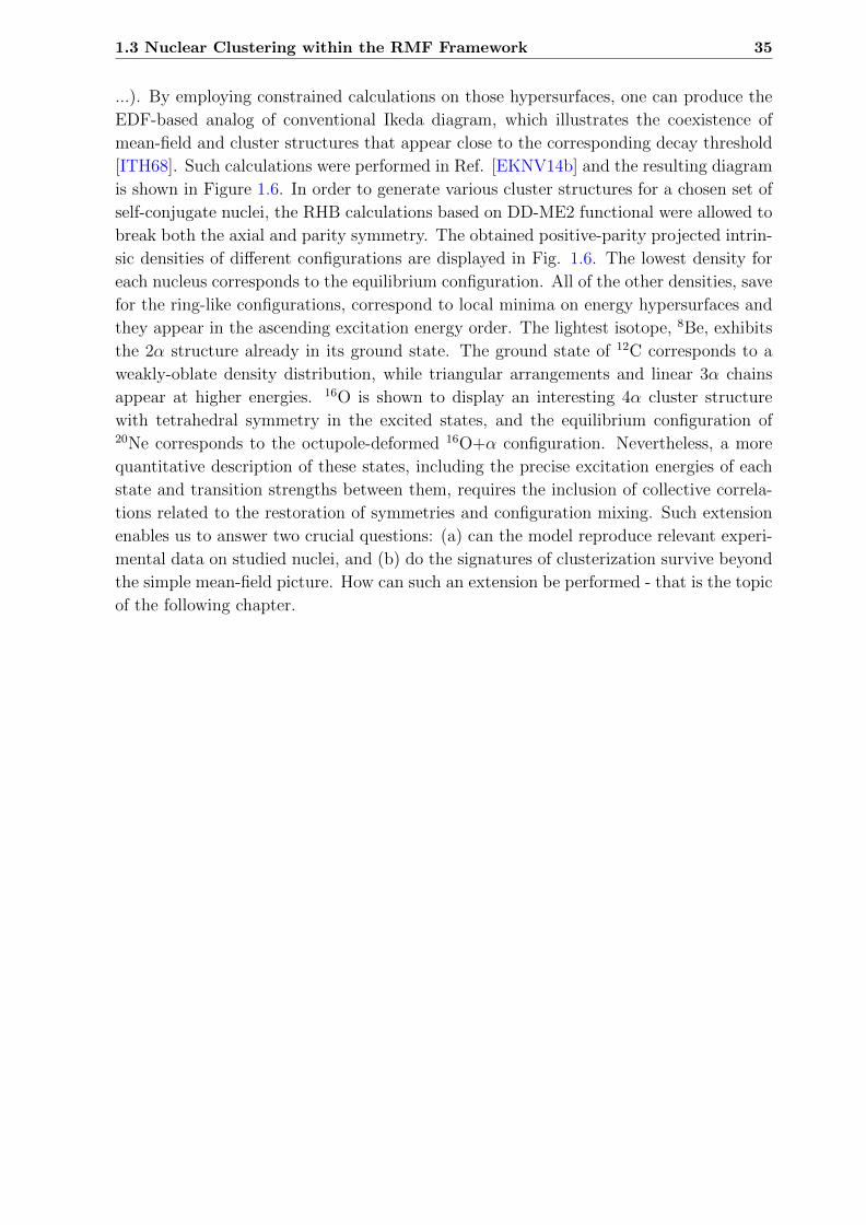
1.3 Nuclear Clustering within the RMF Framework 35
...). By employing constrained calculations on those hypersurfaces, one can produce the
EDF-based analog of conventional Ikeda diagram, which illustrates the coexistence of
mean-field and cluster structures that appear close to the corresponding decay threshold
[ITH68]. Such calculations were performed in Ref. [EKNV14b] and the resulting diagram
is shown in Figure 1.6. In order to generate various cluster structures for a chosen set of
self-conjugate nuclei, the RHB calculations based on DD-ME2 functional were allowed to
break both the axial and parity symmetry. The obtained positive-parity projected intrin-
sic densities of different configurations are displayed in Fig. 1.6. The lowest density for
each nucleus corresponds to the equilibrium configuration. All of the other densities, save
for the ring-like configurations, correspond to local minima on energy hypersurfaces and
they appear in the ascending excitation energy order. The lightest isotope, 8Be, exhibits
the 2α structure already in its ground state. The ground state of 12C corresponds to a
weakly-oblate density distribution, while triangular arrangements and linear 3α chains
appear at higher energies. 16O is shown to display an interesting 4α cluster structure
with tetrahedral symmetry in the excited states, and the equilibrium configuration of20Ne corresponds to the octupole-deformed 16O+α configuration. Nevertheless, a more
quantitative description of these states, including the precise excitation energies of each
state and transition strengths between them, requires the inclusion of collective correla-
tions related to the restoration of symmetries and configuration mixing. Such extension
enables us to answer two crucial questions: (a) can the model reproduce relevant experi-
mental data on studied nuclei, and (b) do the signatures of clusterization survive beyond
the simple mean-field picture. How can such an extension be performed - that is the topic
of the following chapter.


Chapter 2
Restoration of Symmetries and
Configuration Mixing
Symmetry, as wide or narrow as you may define its meaning, is one idea by which man
through the ages has tried to comprehend and create order, beauty, and perfection.
Hermann Weyl, ”Symmetry”
Basic implementation of the nuclear EDF framework is realized in terms of the mean-
field approximation. The very notion of mean-field is closely related to the concept of
spontaneous breaking of symmetries of nuclear Hamiltonian [DS10, RS80], which enables
us to grasp many correlations in a relatively simple manner. However, the resulting many-
body state, rather than carrying good quantum numbers, corresponds to a symmetry-
broken wave packet of states with good quantum numbers. It is well known that a true
spontaneous symmetry breaking can occur only in infinite systems. In finite systems
such as atomic nuclei, on the other hand, quantum fluctuations will eventually cause a
symmetry-breaking wave packet to relax into one of the eigenstates of nuclear Hamil-
tonian. Therefore, these wave packets provide us with only an approximate description
of nuclear system, and broken symmetries ultimately need to be recovered. Restoration
of symmetries is typically carried out by applying techniques rooted in the group theory
[Ham62, RS80], and by considering linear combinations of symmetry-breaking states that
are rotated in a phase space related to the corresponding symmetry group. In order to
account for the magnitude of symmetry breaking as well, a linear combination of dif-
ferent symmetry-restored states is further constructed within the configuration mixing
scheme. This step is formally equivalent to the generator coordinate method (GCM) by
Hill, Wheeler, and Griffin [HW53, GW57], with multipole deformation moments, pairing
degree of freedom, or radii typically playing the role of collective coordinates. These two
steps combined comprise the multi-reference EDF (MR-EDF) framework.
37

38 Chapter 2 Restoration of Symmetries and Configuration Mixing
Collective MR-EDF models, based on both the non-relativistic and relativistic effec-
tive interactions, currently represent state-of-the-art tool for nuclear structure studies
(for detailed discussions see reviews in Refs. [BHR03, NVR11, Egi16, RRR18] and
references cited therein). Virtually all modern MR-EDFs include the axially symmet-
ric quadrupole deformation as a generating coordinate within the configuration mixing
scheme [BFH03, RGER03, NVR06b]. Motivation for this is rather obvious: spherical
shapes can account for only a small number of nuclides at magic nucleon numbers, while
all the other areas of nuclide chart can only be accessed by allowing for the rotational sym-
metry to be broken. Simultaneous breaking of rotational and axial symmetry additionally
extends the reach of a collective model, and within the past decade MR-EDF calculations
based on axial and triaxial quadrupole-deformed shapes have been successfully performed
[BH08, RE10]. More recently, studies that use axially symmetric quadrupole and octupole
deformations as generating coordinates have been reported as well [BRR16, ZYL+16]. On
the other hand, configuration-mixing symmetry-restoring calculations that would allow
for simultaneous breaking of rotational, axial, and parity symmetry are yet to be per-
formed. Besides breaking and restoring of spatial symmetries, another relevant degree
of freedom is provided by pairing correlations, that induce the violation of particle num-
ber invariance in nuclear systems. The vast majority of present MR-EDF models takes
into account only phase fluctuations of pairing correlations through the restoration of
good particle number, while fluctuations in the corresponding magnitude are typically
neglected. Nonetheless, these fluctuations can also be accounted for by using the particle
number dispersion as a collective degree of freedom in the configuration mixing scheme
[VER13, ZLN+16]. Finally, very recent extension of the MR-EDF framework included,
in addition to the axial and triaxial quadrupole deformations, the cranking frequency
as a collective coordinate [EBR16]. Such extension is proposed to cure the well-known
deficiency of overly stretched collective spectra that is a byproduct of the standard pro-
cedure of rotational symmetry restoration. Overall, the choice of appropriate generating
coordinates in configuration mixing calculations is primarily determined by properties of
the nucleus under consideration. However, the required computational time grows rapidly
with increasing the number of generating coordinates. This fact has so far limited prac-
tical implementations of the MR-EDF framework to only two (in majority of cases) or
at most three (exceptionally) generating coordinates at a time. In addition to studies
of even-even nuclei that are routinely performed, the MR-EDF framework was recently
extended to account for odd nuclear systems as well [BABH14, BE16].
In this chapter, we will introduce the MR-EDF framework based on restoration of sym-
metries of RHB states and the subsequent configuration mixing. In Section 2.1, we will
start with some general remarks on breaking and restoring of symmetries in nuclear sys-
tems and the underlying formalism rooted in group theory. Rotational symmetry, particle
number symmetry, and parity symmetry that are particularly relevant for this work will
be discussed in some more detail. Section 2.2 first summarizes basic principles of the con-
figuration mixing scheme based on Hill-Wheeler-Griffin’s framework and then proceeds to
discuss the specific realization of the framework in terms of mixing of symmetry-restored
RHB configurations. Method for deriving and solving the HWG equation, evaluation of
corresponding norm overlap and Hamiltonian kernels, as well as the calculation of various
observables that can be compared to experiment will all be addressed.

2.1 Restoration of Broken Symmetries 39
2.1. Restoration of Broken Symmetries
2.1.1 Breaking and Restoring Symmetries
Symmetries are fundamental features of physical systems, classical and quantum ones
alike. From the Noether’s theorem to the famous Higgs mechanism, they determine prop-
erties of the system and manifest themselves in the underlying equations of motion. In
simple terms, symmetry is just a name for the operation which leaves the physical system
invariant, that is, which transforms it into a state that is completely indistinguishable
from the original one. For example, the ground state of an even-even nucleus in its labo-
ratory frame is invariant under spatial rotations: whatever1 one does with this tiny ball
of quantum liquid it will remain exactly the same. Formally, each symmetry is associated
with the corresponding operator X. System is said to be symmetric under transforma-
tion induced by X if X commutes with Hamiltonian of the system, that is,[X,H
]= 0.
For nuclear systems, set of operators X corresponds to the translational, rotational,
particle number, parity, parity number, and time-reversal symmetries that are exactly
preserved by the nuclear interaction. In addition, isospin invariance is an approximate
symmetry in atomic nuclei, since a weak symmetry breaking is induced by the electro-
magnetic interaction between protons. The true wave function of the system should
correspond to the eigenstate of operators X and, consequently, carry good quantum
numbers related to each of those symmetries (good linear and angular momenta, number
of particles, ...). However, imposing such severe restrictions on our trial wave functions
within the variational procedure of SR-EDF would seriously limit the available variational
space. For example, if we require our trial wave function of Slater or Bogoliubov type to
obey the translational symmetry, the only possible solution would be a pure plane wave
function. Not much in nuclear physics can be described with plane waves. Therefore,
an alternative approach is usually adopted, where a system is allowed to deform and
break symmetries of nuclear Hamiltonian. The breaking of each symmetry is guided by
the corresponding order parameter, g = |g|eiϕg , where |g| and ϕg denote the magnitude
and phase of the order parameter, respectively. The concept of spontaneous symmetry
breaking is schematically depicted in Figure 2.1, where we show the energy of the system
as a function of magnitude |g| and phase ϕg of the order parameter. For |g| = 0, a
symmetry-conserving state is obtained. By allowing for fluctuations in magnitude of the
order parameter, an absolute minimum can be found at configuration |gmin| 6= 0 which
does not anymore possess good symmetry of nuclear Hamiltonian. Additionally, the en-
ergy of this symmetry-broken state is independent of the phase of the order parameter
ϕg. Restoration of symmetries explores the Mexican hat potential in the azimuthal direc-
tion, by combining states with different phases of the order parameter. This accounts to
transition from the intrinsic frame of reference, characterized by a deformed nucleus that
is not under influence of any restoring force such as rotation, to the laboratory frame of
reference, where numerous observables of symmetry-conserving state can be calculated.
1Unless, I guess, you try smashing it against the wall. However, I advise you strongly against doingthis and, even if you did it, no one would know how to write down the corresponding operator anyway.
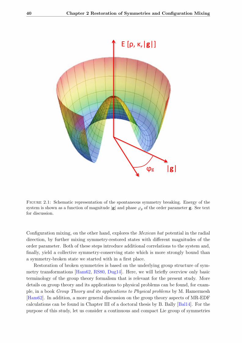
40 Chapter 2 Restoration of Symmetries and Configuration Mixing
|g| ϕg
E [ρ, κ,|g|]
Figure 2.1: Schematic representation of the spontaneous symmetry breaking. Energy of thesystem is shown as a function of magnitude |g| and phase ϕg of the order parameter g. See textfor discussion.
Configuration mixing, on the other hand, explores the Mexican hat potential in the radial
direction, by further mixing symmetry-restored states with different magnitudes of the
order parameter. Both of these steps introduce additional correlations to the system and,
finally, yield a collective symmetry-conserving state which is more strongly bound than
a symmetry-broken state we started with in a first place.
Restoration of broken symmetries is based on the underlying group structure of sym-
metry transformations [Ham62, RS80, Dug14]. Here, we will briefly overview only basic
terminology of the group theory formalism that is relevant for the present study. More
details on group theory and its applications to physical problems can be found, for exam-
ple, in a book Group Theory and its applications to Physical problems by M. Hamermesh
[Ham62]. In addition, a more general discussion on the group theory aspects of MR-EDF
calculations can be found in Chapter III of a doctoral thesis by B. Bally [Bal14]. For the
purpose of this study, let us consider a continuous and compact Lie group of symmetries

2.1 Restoration of Broken Symmetries 41
Table 2.1: Basic properties of nuclear symmetries that are broken and restored within ourcalculation: rotational invariance, particle number invariance, and parity invariance. We listthe underlying groups, corresponding quantum numbers, parameters of groups, operators thatgenerate transformation, irreducible transformations, as well as their respective dimensions. Seetext for more details.
symmetry rotational particle number parity
broken bydeformation
(any multipole)
pairing or
finite temperature
deformation
(odd multipoles)
group G SO(3) U(1) Iπ ≡ 1, Π
quantum numberangular momentum
J
particle numbers
N and Z
parity
π
parameters g α, β, γ ϕN , ϕZ -
operators U e−iαJze−iβJye−iγJz eiϕN NeiϕZ Z 1, Π
irreps Sλab(g) DJMK(α, β, γ), J ∈ N eiϕN,Zm,m ∈ Z Dp(I), p ∈ −1, 1
irreps dimension dλ 2J + 1 1 1
G = R(g). Elements of the symmetry group R(g) commute with the nuclear Hamilto-
nian,[R(g), H
]= 0, and they are parameterized by a set of real parameters g defined
over domain DG. Generators of symmetry transformations U are unitary operators act-
ing on the Hilbert space that can be built as the exponential maps of the symmetry
group elements. Furthermore, one introduces the irreducible representations (irreps) of
the symmetry group, Sλab(g). They are unitary and orthogonal, have dimension dλ, and
are labeled by eigenvalues λ of the corresponding Casimir operator. This enables us to
decompose any function f(g) defined over DG in terms of the irreps of the corresponding
group:
f(g) =∑λab
fλabSλab(g), (2.1)
with fλab as expansion coefficients, and a, b ∈ 1, ..., dλ. Projectors onto good quantum
numbers, that are to be applied on symmetry-broken states, can be built by taking linear
combination of generating operators U multiplied by the corresponding irreps Sλab(g) and
with the appropriate integration (de Haar) measure. In Table 2.1 we summarize basic
properties of nuclear symmetries that are broken and restored within our calculation:
rotational invariance, particle number invariance, and parity invariance. In the following
subsections we will analyze each of them separately.

42 Chapter 2 Restoration of Symmetries and Configuration Mixing
2.1.2 Rotational Symmetry
Among nuclear symmetries that are broken on a SR-EDF level, rotational symmetry is
arguably the most relevant one. Spontaneous breaking of rotational symmetry appears in
all nuclei where neither neutron or proton number is magical, and it has as a consequence
the undesired property that the obtained state does not carry good quantum number of
total angular momentum J . This is at odds with the empirical fact that the energy of an
isolated (rotationally invariant) nucleus does not change under rotations. The underlying
group SO(3) (or, more broadly, SU(2)) is continuous and Lie group of symmetries, with
three spatial Euler angles Ω ≡ (α, β, γ) playing the role of group parameters. Operator
that projects the intrinsic state on a state with good values of angular momentum (AM)
reads:
P JMK =
2J + 1
16π2
∫ 2π
0
dα
∫ π
0
dβ sin β
∫ 4π
0
dγDJ∗MK(α, β, γ)R(α, β, γ), (2.2)
where DJMK(α, β, γ) denotes Wigner D-matrix [VMK88], and the rotation operator reads:
R(α, β, γ) = e−iαJze−iβJye−iγJz . (2.3)
Wigner D-matrix, an irrep of the SO(3) symmetry group, corresponds to matrix elements
of the rotation operator:
DJMK(α, β, γ) = 〈JM |R(α, β, γ)|JK〉 (2.4)
where |JM〉 denotes a many-body state that is an eigenstate of the total angular momen-
tum operator squared, J2, and the z-component of total angular momentum operator,
Jz, simultaneously. The projection operator can then be decomposed in terms of these
symmetry-conserving states:
P JMK =
∑α
|JMα〉 〈JMα| , (2.5)
where index α2 additionally encapsulates all of the remaining quantum numbers that are
necessary to unambiguously define a state. In addition, projection operator satisfies the
following relations:
P JMKP
J ′
M ′K′ = δJJ ′δM ′KPJMK′ ,
(P JMK)† = P J
KM .(2.6)
2A few rows above α represented the Euler angle, which may cause some confusion. However, as it willbecome apparent a few rows below, axial symmetry excludes angles α and γ from the further analysis.Therefore, we reclaim these handy Greek letters to denote other quantities further on in the manuscript.

2.1 Restoration of Broken Symmetries 43
As can be seen from Eq. (2.2), restoration of a good angular momentum for the most
general RHB state |Φ(qi)〉 requires carrying out integrals over three Euler angles. From a
computational perspective, this is a rather time-consuming task. However, by assuming
axial symmetry of the RHB state:
Jz |Φ(qi)〉 = 0 → eiχJz |Φ(qi)〉 = |Φ(qi)〉 , ∀χ ∈ R, (2.7)
this task can be simplified considerably, since in that case integrals over Euler angles α
and γ can be carried out analytically. Furthermore, the following relation:
e−iβJy = eiπ2Jze−iβJxe−i
π2Jz , (2.8)
combined with the axial symmetry property of the RHB state (2.7), can be used to finally
write down the rotation operator as:
R(β) = e−iβJx , (2.9)
which will help us to exploit the self-consistent simplex-x symmetry of intrinsic states
and the consequent block structure of the corresponding U and V matrices. More details
on eigenstates of the simplex-x operator and the expansion of RHB states in the corre-
sponding basis are given in Appendix A. In practical implementations, we will need to
evaluate matrix elements Rαγ(β) of rotation operator in the single-particle basis c†α, cα:
R(β) =∑αγ
Rαγ(β)c†αcγ, (2.10)
where α and γ denote indices of the single-particle basis. Details on calculation of matrix
elements Rαγ(β) in the simplex-x basis are also given in Appendix A.
2.1.3 Particle Number Symmetry
Particle number symmetry is broken in all but doubly magic nuclei. As a consequence
of introducing pairing correlations to the system through the Bogoliubov transformation,
the RHB states are not eigenstates of proton and neutron number operators. Since
an isolated atomic nucleus has a well-defined (integer) number of nucleons, the particle
number symmetry obviously needs to be restored. The underlying group of symmetries,
U(1), is compact, Abelian, and unitary group of degree 1, with gauge angle ϕ ∈ [0, 2π]
playing the role of a group parameter. Operators that project the intrinsic state on a
state with a good particle number (PN) read:

44 Chapter 2 Restoration of Symmetries and Configuration Mixing
PN =1
2π
∫ 2π
0
dϕNei(N−N0)ϕN , PZ =
1
2π
∫ 2π
0
dϕZei(Z−Z0)ϕZ , (2.11)
where N0 (Z0) is the desired number of neutrons (protons), while N (Z) represents the
neutron (proton) number operator:
N =∑α
c†N,αcN,α, Z =∑α
c†Z,αcZ,α. (2.12)
Here, sets of operators c†N,α, cN,α (c†Z,α, cZ,α) correspond to the single-neutron (single-
proton) creation and annihilation operators. The irreducible representation of U(1) sym-
metry group in each isospin channel is one-dimensional, and it corresponds to a matrix
element of the operator that rotates the intrinsic state in a gauge space:
eiϕNN0 = 〈N0|eiϕN N |N0〉 , eiϕZZ0 = 〈Z0|eiϕZ Z |Z0〉 , (2.13)
where |N0〉 and |Z0〉 denote a many-body state that is an eigenstate of the neutron number
and proton number operator, respectively. Projection operators can be decomposed in
terms of these states:
PN =∑α
|N0α〉 〈N0α| , PZ =∑α
|Z0α〉 〈Z0α| (2.14)
where index α again encapsulates all of the remaining quantum numbers that are nec-
essary to unambiguously define a state. Furthermore, projection operators satisfy the
standard relations:
(PN,Z)† = PN,Z , (PN,Z)2 = PN,Z . (2.15)
In practical implementations, integration interval of projection operators (2.11) can be
reduced to [0, π] using the property of good number parity of the intrinsic state. The
resulting integral is further discretized using the Fomenko expansion [Fom70]:
PNτ =1
Nϕ
Nϕ∑l=1
eiϕl(Nτ−Nτ 0), ϕl =π
Nϕ
l, Nτ = N,Z. (2.16)
We note that in the present work we employ the projection after variation (PAV) version
of symmetry restoration, both for the angular momentum projection (AMP) and for the
particle number projection (PNP). Within the PAV framework, the RHB energy is first
minimized and the resulting wave function is subsequently projected on good quantum
numbers. This approach is different from the variation after projection (VAP) technique,

2.1 Restoration of Broken Symmetries 45
where one directly minimizes the projected energy in each variational step. Due to a huge
computational cost of AM-VAP calculations, the AM-PAV has been a conventional choice
in virtually all MR-EDF calculations. The price to pay is the fact that such variational
procedure favors J = 0 state, while higher angular momenta are increasingly less favored,
which stretches the obtained spectra. This anomaly can be accounted for through the
inclusion of cranking frequency as a generating coordinate in the configuration mixing
calculations [EBR16]. On the other hand, PN-VAP calculations are computationally
less demanding than AMP-VAP calculations, and they have been repeatedly performed
within the non-relativistic framework [AER01, SDK+07]. The simpler PN-PAV frame-
work arguably grasps less pairing correlations and provides inferior description in the
weak pairing regime, but it still represents significantly more economical approach from
the computational perspective and it will therefore be employed throughout this study.
2.1.4 Parity Symmetry
Breaking of parity symmetry is related to the non-vanishing value of the lowest odd-
multipolarity electric moment, that is, the electric octupole moment. Microscopically,
octupole collectivity is driven by the existence of pairs of opposite-parity single-particle
orbitals near Fermi surface with angular momenta ∆l = 3 that are strongly coupled
through octupole interaction [BN96]. Even though signatures of octupole collectivity and
the corresponding excitations can be detected and studied over the entire nuclide chart
[RB11], strong experimental traces of octupole collectivity have only recently been ob-
served in 224Ra [G+13] and 144Ba [B+16] isotopes. Among lighter nuclei, the expected
α-clustering in parity-doublets of 20Ne [RB11, EKNV14b] makes breaking of parity in-
variance the necessary ingredient of any theoretical model that aims to comprehensively
describe this isotope. From the group theory perspective, the underlying group of sym-
metries is finite and Abelian, comprising of only two elements: the identity operator 1
and the parity operator Π. This makes the parity projection by far the easiest one to
perform. The operator that projects the intrinsic state on a state with good parity reads:
Pπ =1
2(1+ πΠ), (2.17)
where the quantum number of parity can take only two values, π = ±1. In practical
implementations, restoration of good parity quantum number of the RHB state |Φ(q)〉,q = β2, β3, can be performed following two different prescriptions. The first option is
to calculate the operator (2.17) in a single-particle basis of choice (typically the harmonic
oscillator basis) and directly apply it on a symmetry-broken state |Φ(β2, β3)〉. That way,
one avoids having to carry out separate minimization procedure for RHB states with
negative values of octupole deformation parameter, |Φ(β2,−|β3|)〉. The alternative option
is to calculate RHB states with both positive and negative β3 values, and then use the
virtue of configuration mixing in order to restore good parity of collective states without
ever explicitly applying the projection operator. The equivalence of the two approaches

46 Chapter 2 Restoration of Symmetries and Configuration Mixing
can be demonstrated rather easily. First, we take into account that the parity operator
Π flips the sign of β3 value of the RHB state:
Π |Φ(β2, β3)〉 = |Φ(β2,−β3)〉 . (2.18)
Then by simply applying the projection operator (2.17) on the RHB state with a positive
β3 value:
|Ψπ〉 = Pπ |Φ(β2, |β3|)〉 =1
2(|Φ(β2, |β3|)〉+ π |Φ(β2,−|β3|)〉), (2.19)
one obtains the parity-conserving state, with either positive (π = +1) or negative (π =
−1) parity. The state |Ψπ〉 obviously corresponds to a linear combination of two RHB
states with positive and negative β3 values, which proves the asserted equivalence. In this
work, we will adopt the latter prescription and restore the parity symmetry by using the
reflection-symmetric basis, that is, by ensuring that for each |Φ(β2, |β3|)〉 state the basis
always contains the corresponding |Φ(β2,−|β3|)〉 state as well.
2.1.5 Translational Symmetry
Finally, localization of nuclear mean-field causes breaking of the translational invariance
in all atomic nuclei. However, the exact projection on good values of linear momentum
is notoriously numerically expensive [MFH84], particularly when combined with restora-
tions of other symmetries such as the rotational symmetry. Consequently, restoration of
translational symmetry is usually accounted for in an approximate manner. One of the
most common center-of-mass corrections corresponds to adding the expectation value:
Ec.m. = −〈P2c.m.〉
2mA(2.20)
to the total energy, where Pc.m. is the total momentum of a nucleus with A nucleons.
Validity of this approximation increases with the increase of nucleon number A, and it fi-
nally vanishes for infinite nuclear systems. The expression (2.20) can be further simplified
by evaluating it analytically within the harmonic oscillator approximation [BRRM00]:
EHOc.m. = −3
441A−1/3 MeV. (2.21)
The correction of Eq. (2.21) will be used in the present study. This expression is constant
for each nucleus, that is, it does not depend on the many-body wave function. Therefore,
it will not affect the variational equations and it can be added a posteriori to the energy
of the symmetry-restored collective state. More details on the restoration of translational
symmetry can be found in Refs. [BRRM00, BHR03] and references cited therein.

2.2 Configuration Mixing Scheme 47
2.2. Configuration Mixing Scheme
2.2.1 Basic Principles of the Hill-Wheeler-Griffin’s Method
The generator coordinate method (GCM) theory by Hill, Wheeler, and Griffin [HW53,
GW57] is one of the most widely used methods for describing large amplitude collective
motion of fermionic systems [RS80]. It is a variational method within which a collective
state of quantum system is constructed as a linear combination of many different product
wave functions. In particular, the GCM ansatz for a collective state of quantum system
reads [RS80, Won70, Lat74]:
|Ψα〉 =
∫dθfα(θ) |Φ(θ)〉 , (2.22)
where |Φ(θ)〉 denotes generating intrinsic functions, conveniently chosen for a problem
under consideration, while fα(θ) are weight functions yet to be determined through the
variational procedure. Both generating functions and weight functions depend on θ, a
set of parameters called generating coordinates. Generating coordinates can in principle
be complex [Lat74] and, therefore, integral in (2.22) should run over all corresponding
real and imaginary parts. Finally, label α encapsulates all the relevant quantum numbers
of a collective state. Energy of the collective state (2.22), whose dynamics is governed by
a Hamiltonian operator H, is a functional of weight functions:
Eα[fα] =
∫dθ∫dθ′f ∗α(θ)H(θ, θ′)fα(θ′)∫
dθ∫dθ′f ∗α(θ)N (θ, θ′)fα(θ′)
, (2.23)
where two Hermitian objects have been introduced, namely the Hamiltonian kernel:
H(θ, θ′) = 〈Φ(θ)|H|Φ(θ′)〉 , (2.24)
and the norm overlap kernel:
N (θ, θ′) = 〈Φ(θ)|Φ(θ′)〉 . (2.25)
Weight functions fα(θ) can be determined by applying the variational principle onto the
energy functional (2.23) of a collective state:
δ
δf ∗α(θ)Eα[fα] = 0. (2.26)

48 Chapter 2 Restoration of Symmetries and Configuration Mixing
The corresponding domain of variation is usually kept rather flexible, with the sole re-
quirement being that - whatever weight functions turn out to be - they ultimately yield
normalizable collective states (2.22). Variational principle leads to the Hill-Wheeler-
Griffin (HWG) equation:
∫dθ′[H(θ, θ′)− EαN (θ, θ′)
]fα(θ′) = 0. (2.27)
Formally, the HWG equation has a form of Fredholm integral equation of the first kind
and, together with the collective state normalizability condition, it represents a gener-
alized eigenvalue problem. Solving the HWG equation provides one with the excited
energies Eα of a quantum system, as well as with the corresponding weight functions
fα(θ) that can be used to calculate various observables. Literature on general aspects
of GCM framework is rather abundant [RS80, Won70, Lat74, Lat76]. In the following
subsections, however, we will focus on basic constituents of the particular realization of
the framework that is used in the present study.
2.2.2 Mixing of Symmetry-Restored Configurations
Within our study, a set of generating functions |Φ(θ)〉 is given by a set of product
states that are obtained by solving the RHB equations and additionally projected onto
good values of angular momenta, particle numbers, and parity. Furthermore, generating
coordinates θ correspond to the axially symmetric quadrupole (β2) and octupole (β3)
deformation parameters, and will be denoted as qi ≡ (β2i, β3i) further on. The collective
symmetry-conserving state can therefore be written as:
|ΨJM ;NZ;πα 〉 =
∑i≥0
∑K
fJK;NZ;πα (qi)P
JMKP
N PZP π |Φ(qi)〉 , (2.28)
where a sum in index i runs over a set of RHB states with non-negative values of β3
parameter. Operator that projects on good values of angular momentum P JMK is defined
in Eq. (2.2). As already discussed in Section 2.1.2, the axial symmetry of RHB states
(2.7) enables us to perform integrals over two out of three Euler angles analytically. This
reduces the computational cost significantly but, in turn, restricts the angular momentum
projection to K = 0 components only. Furthermore, operators that project on good values
of particle numbers PN and PZ are defined in Eq. (2.11). In practical implementations,
they are substituted by the corresponding Fomenko expansions of Eq. (2.16). Finally,
technique of projecting on good values of parity has been discussed in Section 2.1.4.
Since the good parity of collective states is recovered by ensuring that the RHB basis is
reflection-symmetric, the corresponding operator P π will not be explicitly written further
on. Rather than that, we extend the sum over index i of Eq. (2.28) by additionally
including states with negative values of β3 parameter, and let the described virtue of

2.2 Configuration Mixing Scheme 49
reflection-symmetric RHB basis do the projecting job for us. The discretized version of
HWG equation within the MR-EDF framework reads:
∑j
[HJ ;NZ;π(qi, qj)− EJ ;NZ;π
α N J ;NZ;π(qi, qj)]fJ ;NZ;πα (qj) = 0. (2.29)
Here, the Hamiltonian kernel HJ ;NZ;π(qi, qj) and the norm overlap kernel N J ;NZ;π(qi, qj)
are defined as:
OJ ;NZ;π(qi, qj) =2J + 1
2δM0δK0
∫ π
0
dβ sin βdJ∗00 (β)1
N2ϕ
Nϕ∑lN=1
Nϕ∑lZ=1
e−iϕlNN0e−iϕlZZ0
× 〈Φ(qi)|Oe−iβJxeiϕlN NeiϕlZ Z |Φ(qj)〉 ,
(2.30)
where dJ∗00 (β) denotes Wigner-d matrix [VMK88], and operator O corresponds to the
identity operator and to the Hamiltonian operator for the norm overlap kernel and the
Hamiltonian kernel, respectively. Details on calculation of these kernels will be discussed
in Section 2.2.4.
The HWG equation in a form of Eq. (2.29) represents a generalized eigenvalue problem.
Consequently, the weight functions fJ ;NZ;πα (qi) do not form an orthogonal set and cannot
be interpreted as collective wave functions for variable qi. Therefore, the first step in
solving the HWG equation is introducing an another set of functions:
gJ ;NZ;πα (qi) =
∑j
(N J ;NZ;π)1/2(qi, qj)fJ ;NZ;πα (qj), (2.31)
that are indeed orthogonal and play the role of collective wave functions. After exchanging
weight functions for the collective wave functions, the HWG equation assumes a form of
the ordinary eigenvalue problem:
∑j
HJ ;NZ;π(qi, qj)gJ ;NZ;πα (qj) = EJ ;NZ;π
α gJ ;NZ;πα (qi), (2.32)
with the modified Hamiltonian kernel:
HJ ;NZ;π(qi, qj) =∑k,l
(N J ;NZ;π)−1/2(qi, qk)HJ ;NZ;π(qk, ql)(N J ;NZ;π)−1/2(ql, qj). (2.33)
The eigenvalue problem for the norm overlap kernel reads:

50 Chapter 2 Restoration of Symmetries and Configuration Mixing
∑j
N J ;NZ;π(qi, qj)uJ ;NZ;πk (qj) = nJ ;NZ;π
k uJ ;NZ;πk (qi), (2.34)
where uJ ;NZ;πk (qi) and nJ ;NZ;π
k are the corresponding eigenvectors and eigenvalues, respec-
tively. Inversion of the norm overlap kernel in Eq. (2.33) is formally possible only if
the kernel matrix does not have any zero eigenvalues. In practical implementations, one
encounters norm eigenvectors with very small eigenvalues, that are a direct consequence
of the fact that the original set of generating functions is not linearly independent. These
states need to be removed from the basis, while the remaining states are used to build
the collective Hamiltonian:
HJ ;NZ;πkl,c =
1√nJ ;NZ;πk
1√nJ ;NZ;πl
∑i,j
uJ ;NZ;πk (qi)HJ ;NZ;π(qi, qj)u
J ;NZ;πl (qj), (2.35)
which can be easily diagonalized using the standard diagonalization techniques:
∑l
HJ ;NZ;πkl,c gJ ;NZ;π
l,α = EJ ;NZ;πα gJ ;NZ;π
k,α . (2.36)
Diagonalization takes place in the collective space spanned by the natural basis states:
|k〉 =1√
nJ ;NZ;πk
∑i
uJ ;NZ;πk (qi)P
J00P
N PZ |Φ(qi)〉 , (2.37)
whose dimension is equal to or smaller than the dimension of the original HWG problem.
Solving the Eq. (2.36) for each value of angular momentum J and parity π separately3
determines both the energy of the ground state and energies of the excited states. We note
that only states with natural spin-parity, that is, states which satisfy the rule (−1)J = π
are accessible with the present model. The collective wave functions gJ ;NZ;πα (qi) and the
weight functions fJ ;NZ;πα (qi) are finally calculated from the eigenfunctions of the norm
overlap as:
gJ ;NZ;πα (qi) =
∑k
gJ ;NZ;πk,α uJ ;NZ;π
k (qi), (2.38)
fJ ;NZ;πα (qi) =
∑k
gJ ;NZ;πk,α√nJ ;NZ;πk
uJ ;NZ;πk (qi). (2.39)
3In principle, one could additionally project on each value of number of neutrons and protons, (N,Z).However, we only project on values (N0, Z0) that correspond to a real nucleus under consideration.

2.2 Configuration Mixing Scheme 51
2.2.3 Structural Properties of Collective States
Collective wave functions of Eq. (2.38) do not represent a physical observable. How-
ever, amplitudes of the collective wave functions squared |gJ ;NZ;πα (qi)|2 manifest the degree
of shape fluctuations in both the quadrupole and octupole directions, and as such they
provide an insight into the structure of collective states in the intrinsic frame. On a
more quantitative level, one can calculate average values of quadrupole and octupole
deformation parameters in the collective state:
〈β2〉J ;NZ;πα =
∑i
|gJ ;NZ;πα (qi)|2β2i, (2.40)
〈|β3|〉J ;NZ;πα =
∑i
|gJ ;NZ;πα (qi)|2|β3i|, (2.41)
where in the octupole direction we have taken an absolute value of deformation parameter
because 〈β3〉 vanishes identically for all states with good parity. These quantities provide
a good indication about the dominant mean-field configurations in a collective state. In
addition, they enable us to characterize the intrinsic density of a collective state by calcu-
lating corresponding RHB densities constrained to the 〈β2〉J ;NZ;πα and 〈|β3|〉J ;NZ;π
α values.
Furthermore, weight functions and collective wave functions can be used to calculate val-
ues of various observables, both in a collective state and between two different collective
states. The most common examples are electric spectroscopic quadrupole moments and
electric multipole transition strengths, that have been routinely calculated within the MR-
EDF framework for decades [RS80, RGER02, Fru07]. Electric spectroscopic quadrupole
moment of the collective state α with total spin-parity Jπ can be computed as:
Qspec2 (Jπα) = e
√16π
5
(J 2 J
J 0 −J
)∑qiqf
fJ ;NZ;π∗α (qf ) 〈Jqf ||Q2||Jqi〉 fJ ;NZ;π
α (qi). (2.42)
The reduced electric transition strength of multipolarity λ between an initial collective
state αi of total spin-parity Jπii and a final collective state αf of total spin-parity Jπff can
be computed as:
B(Eλ; Jπiαi → Jπfαf ) =
e2
2Ji + 1
∣∣∣∑qiqf
fJf ;NZ;πf∗αf (qf ) 〈Jfqf ||Qλ||Jiqi〉 fJi;NZ;πi
αi(qi)∣∣∣2. (2.43)
Quantity 〈Jfqf ||Qλ||Jiqi〉 in Eqs. (2.42) and (2.43) corresponds to the reduced matrix
element of the electric multipole operator Qλµ. More practical details on calculation of
Qspec2 and B(Eλ) can be found in Appendix B.1. Here, we note that all the quantities are

52 Chapter 2 Restoration of Symmetries and Configuration Mixing
calculated in full configurational space. Therefore, there is no need to introduce effective
charges and e always denotes the bare value of the proton charge.
Recently, the MR-EDF framework has been extended by including calculation of tran-
sition densities between low-lying excited states [YBH15]. This extension enables us to
determine form factors for electron scattering off nuclei, that represent a very useful tool
in studies of nuclear density distributions [Wal04, Won98, YBH15]. The longitudinal
form factor for an angular momentum transfer L can be computed as the Fourier-Bessel
transform of the reduced transition density ρJfαfJiαi,L
(r) from an initial state state αi of total
spin-parity Jπii to a final state αf of total spin-parity Jπff :
FL(q) =
√4π
Z
∫ ∞0
drr2ρJfαfJiαi,L
(r)jL(qr), (2.44)
where q denotes momentum transfer and jL(qr) is the spherical Bessel function of the first
kind. The reduced transition density corresponds to the radial part of the 3D transition
density and it can be calculated as:
ρJfαfJiαi,L
(r) = (−1)Jf−Ji2Jf + 1
2Ji + 1
∑K
〈Jf0LK|JiK〉∫
drρJfJiK0αfαi (r)Y ∗LK(r), (2.45)
where Y ∗LK(r) are spherical harmonics and ρJfJiK0αfαi (r) denotes the pseudo GCM density
as defined in [YBH15]. The pseudo GCM density does not represent an observable, but
it can be used to calculate nuclear densities in the laboratory frame:
ρlabα (r) =
∑λ
Yλ0(r) 〈J0λ0|J0〉∑K
〈J0λK|JK〉∫
dr′ρJJK0αα (r, r′)Y ∗λK(r′). (2.46)
More details on calculation of pseudo GCM densities and general aspects of implementing
the electron-nucleus scattering formalism to the present model can be found in Appendix
B.2.
2.2.4 Evaluation of Norm Overlap and Hamiltonian Kernels
Evaluation of the Hamiltonian kernel (2.24) and the norm overlap kernel (2.25) lies at
the very heart of the MR-EDF method. The simplest way of handling the norm overlaps
is approximating them with Gaussian functions [RS80]. This assumption is based on an
observation that the overlap N (θ, θ′) is rapidly decreasing function of distance |θ − θ′|,that is, that the overlap between |Φ(θ)〉 and |Φ(θ′)〉 does not vanish only when θ and θ′
are relatively close to each other. Within the Gaussian overlap approximation (GOA),
the norm overlap therefore reads:

2.2 Configuration Mixing Scheme 53
N (θ, θ′) = e−12γ(χ)(θ−θ′)2 , (2.47)
with the width γ(χ) typically being a function of the center of mass coordinate χ =12(θ + θ′). If one additionally assumes that a ratio between the Hamiltonian kernel and
the norm overlap kernel is a smooth function of generating coordinates, it is possible
to locally expand kernels up to the second order in θ − θ′ variable. In this way, the
HWG equation transforms into the second-order differential (Schrodinger) equation, and
the GCM framework is replaced by the well-known collective Hamiltonian model [RS80,
PR09]. On the other hand, if one decides to remain exact, the overlap between two RHB
states can be calculated using the conventional Onishi formula [OY66, RS80]:
N (θ, θ′) = 〈Φ(θ)|Φ(θ′)〉 =[
det(U †(θ′)U(θ) + V †(θ′)V (θ)
)]1/2, (2.48)
where U(θ) and V (θ) are Bogoliubov wave functions introduced in Chapter 1. The fact
that the Onishi formula yields the sign ambiguity in a case when intrinsic states do not
preserve any discrete symmetries has haunted nuclear community for decades. Various
techniques to bypass this deficiency have therefore been proposed, including the method
of analytical continuation [HHR82] and the Neergard’s method [NW83]. More recently,
an elegant Pfaffian formula based on Grassman algebra that completely resolves the sign
ambiguity has been developed by L. Robledo [Rob09, BR12]. In this work, we will use
the conventional framework of Onishi in order to calculate norm overlaps between the
RHB states. Due to the discrete simplex-x and time-reversal symmetries of the intrinsic
states, the matrix under determinant [see Eq. (2.48)] will exhibit a block structure with
identical blocks, which can be exploited to unambiguously fix the corresponding sign.
In particular, overlap between the RHB state |Φ(qi)〉 and the RHB state |Φ(qj)〉 that
has been rotated by a rotational angle β and a gauge angle ϕ in any of the two isospin
channels reads:
N (qi, qj, β, ϕ) = 〈Φ(qi)|e−iβJxeiϕN |Φ(qj)〉
=[e−iβTr[Jx]+ϕTr[1] detNg(qi, qj, β, ϕ)
] 12 ,
(2.49)
where we have introduced:
Ng(qi, qj, β, ϕ) = e−iϕUT (qi)R∗(β)U∗(qj) + eiϕV T (qi)R(β)V ∗(qj), (2.50)
and R(β) corresponds the matrix of rotation operator in the simplex-x basis, details of
which are given in Appendix A.
Furthermore, the MR-EDF framework can be thought of as an extension of the SR-
EDF framework, where a basic functional ESR-EDF[ρ, κ, κ∗] of intrinsic densities (1.36) has
been replaced by a more general functional EMR-EDF[ρ10, κ10, κ10∗] of transition densities
between different RHB states. In other words, the ground state expectation value of the
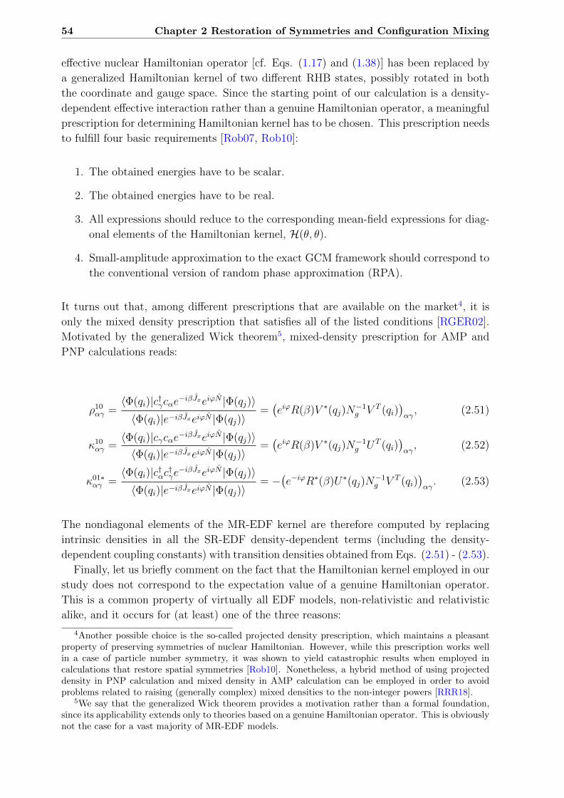
54 Chapter 2 Restoration of Symmetries and Configuration Mixing
effective nuclear Hamiltonian operator [cf. Eqs. (1.17) and (1.38)] has been replaced by
a generalized Hamiltonian kernel of two different RHB states, possibly rotated in both
the coordinate and gauge space. Since the starting point of our calculation is a density-
dependent effective interaction rather than a genuine Hamiltonian operator, a meaningful
prescription for determining Hamiltonian kernel has to be chosen. This prescription needs
to fulfill four basic requirements [Rob07, Rob10]:
1. The obtained energies have to be scalar.
2. The obtained energies have to be real.
3. All expressions should reduce to the corresponding mean-field expressions for diag-
onal elements of the Hamiltonian kernel, H(θ, θ).
4. Small-amplitude approximation to the exact GCM framework should correspond to
the conventional version of random phase approximation (RPA).
It turns out that, among different prescriptions that are available on the market4, it is
only the mixed density prescription that satisfies all of the listed conditions [RGER02].
Motivated by the generalized Wick theorem5, mixed-density prescription for AMP and
PNP calculations reads:
ρ10αγ =
〈Φ(qi)|c†γcαe−iβJxeiϕN |Φ(qj)〉〈Φ(qi)|e−iβJxeiϕN |Φ(qj)〉
=(eiϕR(β)V ∗(qj)N
−1g V T (qi)
)αγ, (2.51)
κ10αγ =
〈Φ(qi)|cγcαe−iβJxeiϕN |Φ(qj)〉〈Φ(qi)|e−iβJxeiϕN |Φ(qj)〉
=(eiϕR(β)V ∗(qj)N
−1g UT (qi)
)αγ, (2.52)
κ01∗αγ =
〈Φ(qi)|c†αc†γe−iβJxeiϕN |Φ(qj)〉〈Φ(qi)|e−iβJxeiϕN |Φ(qj)〉
= −(e−iϕR∗(β)U∗(qj)N
−1g V T (qi)
)αγ. (2.53)
The nondiagonal elements of the MR-EDF kernel are therefore computed by replacing
intrinsic densities in all the SR-EDF density-dependent terms (including the density-
dependent coupling constants) with transition densities obtained from Eqs. (2.51) - (2.53).
Finally, let us briefly comment on the fact that the Hamiltonian kernel employed in our
study does not correspond to the expectation value of a genuine Hamiltonian operator.
This is a common property of virtually all EDF models, non-relativistic and relativistic
alike, and it occurs for (at least) one of the three reasons:
4Another possible choice is the so-called projected density prescription, which maintains a pleasantproperty of preserving symmetries of nuclear Hamiltonian. However, while this prescription works wellin a case of particle number symmetry, it was shown to yield catastrophic results when employed incalculations that restore spatial symmetries [Rob10]. Nonetheless, a hybrid method of using projecteddensity in PNP calculation and mixed density in AMP calculation can be employed in order to avoidproblems related to raising (generally complex) mixed densities to the non-integer powers [RRR18].
5We say that the generalized Wick theorem provides a motivation rather than a formal foundation,since its applicability extends only to theories based on a genuine Hamiltonian operator. This is obviouslynot the case for a vast majority of MR-EDF models.

2.2 Configuration Mixing Scheme 55
1. The effective interaction is density-dependent.
In order to correct for too large incompressibility and properly describe the nuclear
surface properties, virtually all modern EDF parameterizations include at least one
density-dependent term. Most notably, the most successful covariant realizations
of the EDF framework are explicitly built as density-dependent models.
2. Vertices used in ph and pp channel are different and possibly not antisymmetric.
This is particularly the case for Skyrme EDFs, where different vertices were intro-
duced in order to account for too small or even repulsive pairing matrix elements
derived from the original interaction [SBB+13], and for relativistic EDFs, where
a non-relativistic pairing force is typically added to the functional [VALR05]. On
the other hand, Gogny EDFs are characterized by using the same antisymmetrized
vertices everywhere. Nevertheless, it has been argued that their density-dependence
still makes it impossible for the phenomenological functional to be mapped on a
functional that is a strict expectation value of a many-body Hamiltonian [BDL09].
3. The exchange terms of the interaction are either approximated or omitted.
The exact treatment of all exchange terms can increase the required computational
time by an order of magnitude. These terms are therefore often either approximated
by simpler expressions (such as the Slater approximation to the Coulomb exchange
potential) or completely omitted (in case of which their physical effect is accounted
for through the adjustment of phenomenological coupling constants).
The undesired consequence of these approximations is breaking of the exchange symmetry
(Pauli principle), that produces spurious self-interaction and self-pairing contributions to
the nuclear EDF [AER01, DSNR07, DBB+09, LDB09, BDL09]. These non-physical con-
tributions were demonstrated to manifest themselves through divergences and/or finite
steps when considering the symmetry-restored energies as functions of collective coordi-
nates. In particular, while situation in AMP calculations appears to be less severe [Egi16],
the PNP calculations for very large values of discretization points Nϕ were shown to ex-
hibit finite steps and discontinuities whenever a single-particle level crosses the Fermi
energy [BDL09]. One should note that this theoretical drawback is related only to the
employed energy functional, and not to the product states in question. Therefore, even
though they may be affected indirectly, all observables that are calculated as expectation
values of the corresponding genuine operators do not contain any explicit spurious con-
tributions. Research towards spuriousity-free MR-EDF calculations is still in its infancy
and it is currently moving in two separate directions: one of them is development of the
regularization schemes for the existing functionals [LDB09, BDL09] and the other one
is development of the pseudo-potential-based-EDF parameterizations that are a priori
free of spuriousities [SBB+13]. In the meantime, one should stay aware of the existing
theoretical drawbacks and, if possible, try to estimate their influence on predictions of
the respective model.

Part II
Microscopic Description of
Clustering in Light Nuclei
57


Chapter 3
A Computational Interlude
What can be asserted without evidence can be dismissed without evidence.
Christopher Hitchens’ razor
In the preceding chapters we have introduced and described a collective nuclear model
based on the restoration of symmetries of intrinsic states and the subsequent configura-
tion mixing. In the following chapters, this framework will be employed in a study of
clustering phenomena in neon and carbon isotopes. However, before discussing physical
aspects of the study, let us first address some of the issues related to the computational
implementation of the model. In particular, we will address the question of convergence of
results with respect to various discretization parameters, both on the SR-EDF and on the
MR-EDF level. To begin with, computational aspects of the mean-field calculations will
be discussed. The RHB calculations were performed by using the quadrupole-deformed
axially-symmetric version of the DIRHB package [NPVR14] as a starting point, and by
further extending it in order to additionally include the axially-symmetric octupole degree
of freedom. Since the number of required configurations is relatively low (as compared to,
for example, nuclear fission calculations), it is the least time-consuming part of our cal-
culation. In the next step, the restoration of good angular momentum, particle number,
and parity of RHB states were built upon the mean-field code. This step represents the
most time-consuming part of the calculation. The symmetry-restored configurations were
then mixed in order to build the symmetry-conserving collective states and study their
spectroscopic properties. In the second part of this chapter, we will examine convergence
of the obtained projected energies with respect to the number of integration points in
the β-Euler angle and the ϕ-gauge angle. The need for this is (at least) two-fold. First,
as in any other discretized calculation, it is necessary to verify that the particular choice
of mesh provides a satisfactory convergence of calculated quantities. The second reason
is to demonstrate the influence of the theoretical drawback related to the fact that the
59

60 Chapter 3 A Computational Interlude
employed functional does not correspond to the expectation value of a genuine Hamilto-
nian operator (for more details see Section 2.2.4 and references cited therein). Finally, we
will discuss the influence of linear dependence (overcompleteness) of the original set of
RHB basis functions on the output of the model. These linear dependencies are routinely
removed by reducing the size of a natural basis [see Eq. (2.37)] and by verifying that the
obtained spectra is stable with respect to the number of remaining natural basis states.
For the sake of brevity, the entire analysis of this chapter will be based only on a case of20Ne isotope, that we conveniently choose as a representative for a class of light nuclei.
3.1. Convergence of Mean-Field Calculation
Starting point of our calculation is the axially-symmetric quadrupole-deformed version
of the DIRHB package, which computes the ground-state properties of even-even nuclei
using the framework of relativistic self-consistent mean-field models [NPVR14]. This
code was first extended by including the axially-symmetric octupole degree of freedom,
which enabled us to perform self-consistent calculations in the entire β2 − β3 plane. The
RHB equations were solved in the configurational space of axially-symmetric harmonic
oscillator, by expanding the large and the small component of nuclear spinors in bases
of the corresponding eigenfunctions. As already emphasized in Chapter 1, the appear-
ance of spurious states is avoided by choosing quantum numbers |α〉 = |nzn⊥Λms〉 in
such a way that their combination does not exceed the maximal major quantum num-
ber Nsh = 2n⊥ + |Λ| + nz for the large component of nuclear spinor and the maximal
major quantum number Nsh + 1 for the small component of nuclear spinor. Of course,
the convergence of results with respect to the size of basis Nsh has to be verified. There-
fore, in the left panel of Figure 3.1 we plot the differences of calculated RHB binding
energies ∆ENshRHB = ENsh
RHB − ENsh+2RHB of 20Ne isotope for different numbers of oscillator
shells Nsh = 6, 8, 10 in the (β2, β3 > 0) plane1. Dashed contours connect points with the
same ∆ENshRHB values and they are separated by 1 MeV. The constrained RHB equations
were solved on a two-dimensional mesh, by imposing constraints on the axially-symmetric
quadrupole and octupole moments and implementing the augmented Lagrangian method
[SSBN10]. The resulting mesh covers a wide range of deformations in both the quadrupole
and octupole degree of freedom: β2 ∈ [−0.6, 1.5] and β3 ∈ [−2.0, 2.0]. The step size on the
oblate and on the prolate side were taken to be ∆β2 = 0.15 and ∆β2 = 0.3, respectively,
while the step size in the octupole direction equals ∆β3 = 0.2. After solving the RHB
equation, all of the configurations with energy more than 20 MeV above the equilibrium
were removed from the basis. Of course, the exclusion of such high-energy states does
not influence the predictive power of our model which ultimately aims to describe the
low-lying structure of atomic nuclei. The remaining states, which will be included in the
subsequent symmetry restoration and configuration mixing, are denoted with red circles
in the left panel of Fig. 3.1. By inspecting the Fig. 3.1, one can verify that a satisfactory
convergence for all the states is obtained for Nsh = 10 oscillator shells. In particular, a
1The (β2, β3 < 0) plane is equivalent to the (β2, β3 > 0) plane, that is, one can be obtained bymirroring the other one around the β3 = 0 axis.

3.1 Convergence of Mean-Field Calculation 61
−0.5 0.0 0.5 1.0β2
0.0
0.4
0.8
1.2
1.6
2.0β3
1.5
Nsh=6
2 4 6 8 10ENsh
−ENsh−2 [MeV]
−0.5 0.0 0.5 1.0β2
0.0
0.4
0.8
1.2
1.6
2.0
1.5
(a)
Nsh=8
0 1 2 3 4 5 6 7 8 9 10E
Nsh
RHB−ENsh+2
RHB [MeV]
−0.5 0.0 0.5 1.0β2
0.0
0.4
0.8
1.2
1.6
2.0
1.5
Nsh=10
0.4 0.8 1.2 1.6β3
−150
−145
−140
−135
−130
−125
−120
−115
EN
sh
RHB [M
eV]
0.0 2.0
(b)
β2 =1.2
Nsh=6
Nsh=8
Nsh=10
Nsh=12
Figure 3.1: Left panel (a): differences of calculated RHB binding energies ∆ENshRHB = ENshRHB −ENsh+2
RHB of 20Ne isotope for different numbers of oscillator shells Nsh in the (β2, β3 > 0) plane.Dashed contours are separated by 1 MeV. Red points denote calculated configurations that areat most 20 MeV above the equilibrium configuration. Right panel (b): RHB binding energiesof (β2 = 1.2, β3 > 0) configurations for different numbers of oscillator shells Nsh.
shift to 12 oscillator shells brings less than 1 MeV of binding for a large majority of cho-
sen states. Only a small minority of states, predominantly at larger β3 deformations and
on the oblate side of β2 − β3 plane, have converged with ∆ENsh=10RHB > 1 MeV. However,
as it will be demonstrated in the following chapter, this part of the β2 − β3 plane will
not play any relevant role in the description of nuclear collective dynamics. In fact, it
is well established that the absolute value of binding energy does not significantly affect
the collective nuclear motion, as long as the shape of the energy landscape is preserved
[RGER02]. In order to demonstrate this point, in the right panel of Fig. 3.1 we show the
calculated RHB binding energies of (β2 = 1.2, β3 > 0) configurations for different numbers
of oscillator shells Nsh. While the Nsh = 6 and Nsh = 8 values are obviously not suffi-
cient to obtain a proper convergence, especially for larger β3 deformations, the Nsh = 10
and Nsh = 12 curves indeed exhibit almost identical shape. Similar conclusions can be
drawn if one inspects the corresponding plots for other considered isotopes. Therefore, a
value of Nsh = 10 oscillator shells is adopted in solving RHB equations for all the further
calculations. The resulting wave functions are first obtained in the configurational space
of harmonic oscillator, and they are subsequently used to calculate densities in the same
configurational space. These densities are then transformed to the cylindrical coordinate
space (r⊥, z, φ), where they are employed to compute various terms of the energy density
functional. Discretization in the z− and r⊥− directions have been carried out following
the Gauss-Hermite and Gauss-Laguerre quadrature methods, respectively, and the corre-
sponding number of points equal NGH = 16 and NGL = 14, respectively. Computational
time required to compute one RHB configuration will depend on its distance from the
absolute minimum. For configurations with reasonable binding energies (that is, at most
20 MeV above the absolute minimum) and Nsh = 10 oscillator shells, depending on the
machine, the required computational time will typically range between ten and thirty
seconds. Of course, increasing the size of a single-particle basis will significantly increase
the required computational time, both for the SR-EDF and for the MR-EDF calculation.

62 Chapter 3 A Computational Interlude
−0.5 0.0 0.5 1.0
0.40.81.21.6
β3
0.0
2.0Nβ=15
Jπ =0+
0.000.150.300.450.600.750.901.051.201.351.50
−0.5 0.0 0.5 1.0
0.4
0.8
1.2
1.6
Nβ=19
Jπ =0+
−0.5 0.0 0.5 1.0
0.4
0.8
1.2
1.6
Nβ=23
Jπ =0+
−0.5 0.0 0.5 1.0
0.4
0.8
1.2
1.6
Nβ=27
Jπ =0+
0.00
0.06
0.12
0.18
0.24
−0.5 0.0 0.5 1.0
0.40.8β
3
0.0
1.21.62.0
Nβ=15
Jπ =2+
−0.5 0.0 0.5 1.0
0.4
0.8
1.2
1.6
Nβ=19
Jπ =2+
−0.5 0.0 0.5 1.0
0.4
0.8
1.2
1.6
Nβ=23
Jπ =2+
−0.5 0.0 0.5 1.0
0.4
0.8
1.2
1.6
Nβ=27
Jπ =2+
0.00
0.06
0.12
0.18
0.24
−0.5 0.0 0.5 1.0
0.40.8β
3
0.0
1.21.62.0
Nβ=15
Jπ =4+
−0.5 0.0 0.5 1.0
0.4
0.8
1.2
1.6
Nβ=19
Jπ =4+
−0.5 0.0 0.5 1.0
0.4
0.8
1.2
1.6
Nβ=23
Jπ =4+
−0.5 0.0 0.5 1.0
0.4
0.8
1.2
1.6
Nβ=27
Jπ =4+
0.00
0.06
0.12
0.18
0.24
−0.5 0.0 0.5 1.0β2
0.40.8β
3
1.50.0
1.21.62.0
Nβ=15
Jπ =6+
−0.5 0.0 0.5 1.0β2
0.4
0.8
1.2
1.6
1.5
Nβ=19
Jπ =6+
−0.5 0.0 0.5 1.0β2
0.4
0.8
1.2
1.6
1.5
Nβ=23
Jπ =6+
−0.5 0.0 0.5 1.0β2
0.4
0.8
1.2
1.6
1.5
Nβ=27
Jπ =6+
0.0
0.3
0.6
0.9
1.2
|ENβ
proj−E
Nβ+4
proj
|[MeV
]
Figure 3.2: Absolute energy differences ∆ENβproj = |ENβproj−E
Nβ+4proj | of states projected on even-
positive spin-parities for different numbers of β−Euler angle mesh points Nβ. Separation ofdashed lines on all panels corresponds to the separation of neighboring ticks on their respectivecolorbars, that is, to 0.06, 0.06, 0.06, 0.3 MeV for Jπ = 0+, 2+, 4+, 6+, respectively. Red circlesdenote configurations that are included in the symmetry restoration and configuration mixingcalculation. Results are shown for 20Ne isotope. See text for more details.
3.2. Convergence of Symmetry-Restoring Calculation
3.2.1 Convergence of Projected Energies
Restoration of broken symmetries of the RHB states and the subsequent configura-
tion mixing represent the most numerically-involved part of our calculation. The reason
for this is rather obvious: while the SR-EDF is a functional of (normal and anoma-
lous) density matrices, the MR-EDF can be seen as a more general functional of all
the transition density matrices. This means that, starting from NSR-EDF states in the
RHB basis, all of the relevant symmetry-restored quantities have to be calculated for
NMR-EDF = NSR-EDF(NSR-EDF + 1)/2 configurations. Formally, these quantities represent
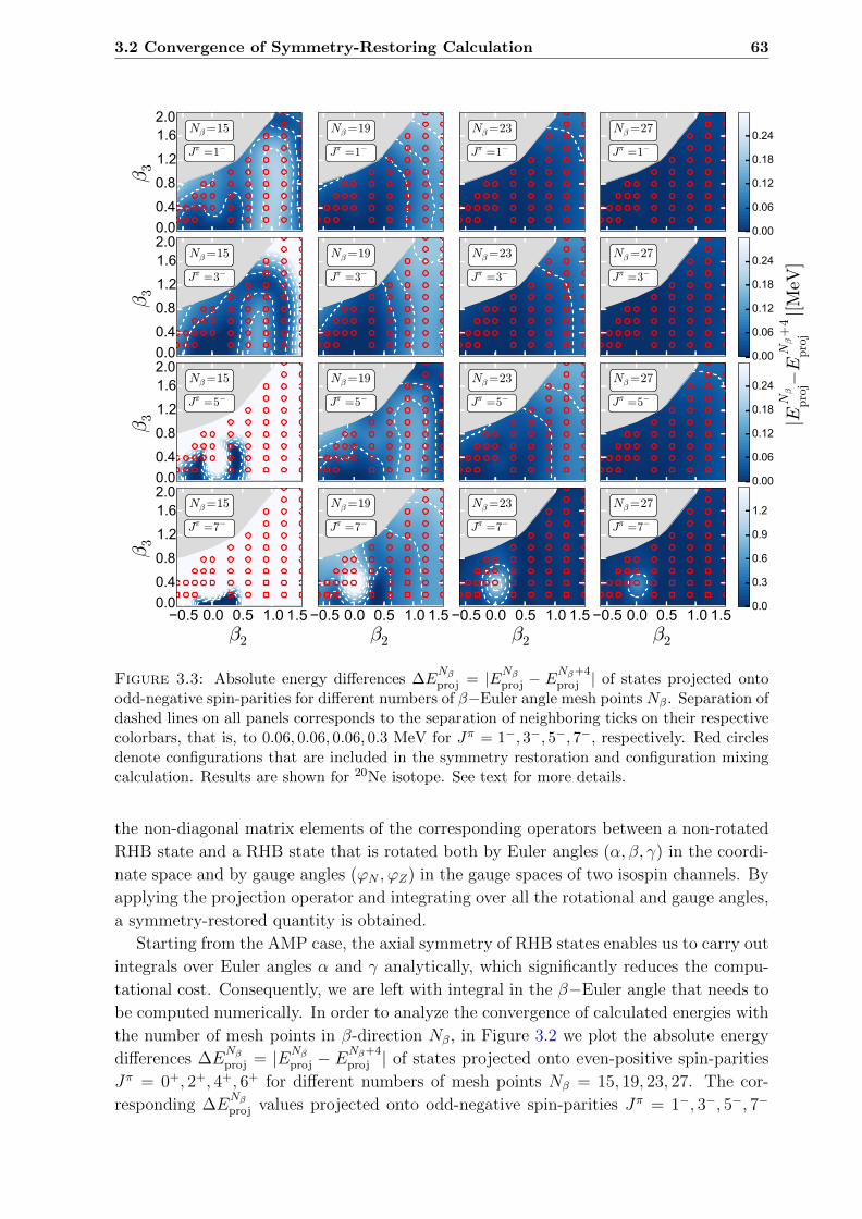
3.2 Convergence of Symmetry-Restoring Calculation 63
−0.5 0.0 0.5 1.0
0.40.81.21.6
β3
0.0
2.0Nβ=15
Jπ =1−
0.000.150.300.450.600.750.901.051.201.351.50
−0.5 0.0 0.5 1.0
0.4
0.8
1.2
1.6
Nβ=19
Jπ =1−
−0.5 0.0 0.5 1.0
0.4
0.8
1.2
1.6
Nβ=23
Jπ =1−
−0.5 0.0 0.5 1.0
0.4
0.8
1.2
1.6
Nβ=27
Jπ =1−
0.00
0.06
0.12
0.18
0.24
−0.5 0.0 0.5 1.0
0.40.81.21.6
β3
0.0
2.0Nβ=15
Jπ =3−
−0.5 0.0 0.5 1.0
0.4
0.8
1.2
1.6
Nβ=19
Jπ =3−
−0.5 0.0 0.5 1.0
0.4
0.8
1.2
1.6
Nβ=23
Jπ =3−
−0.5 0.0 0.5 1.0
0.4
0.8
1.2
1.6
Nβ=27
Jπ =3−
0.00
0.06
0.12
0.18
0.24
−0.5 0.0 0.5 1.0
0.40.81.21.6
β3
0.0
2.0Nβ=15
Jπ =5−
−0.5 0.0 0.5 1.0
0.4
0.8
1.2
1.6
Nβ=19
Jπ =5−
−0.5 0.0 0.5 1.0
0.4
0.8
1.2
1.6
Nβ=23
Jπ =5−
−0.5 0.0 0.5 1.0
0.4
0.8
1.2
1.6
Nβ=27
Jπ =5−
0.00
0.06
0.12
0.18
0.24
−0.5 0.0 0.5 1.0β2
0.40.81.21.6
β3
1.50.0
2.0Nβ=15
Jπ =7−
−0.5 0.0 0.5 1.0β2
0.4
0.8
1.2
1.6
1.5
Nβ=19
Jπ =7−
−0.5 0.0 0.5 1.0β2
0.4
0.8
1.2
1.6
1.5
Nβ=23
Jπ =7−
−0.5 0.0 0.5 1.0β2
0.4
0.8
1.2
1.6
1.5
Nβ=27
Jπ =7−
0.0
0.3
0.6
0.9
1.2
|ENβ
proj−E
Nβ+4
proj
|[MeV
]
Figure 3.3: Absolute energy differences ∆ENβproj = |ENβproj − E
Nβ+4proj | of states projected onto
odd-negative spin-parities for different numbers of β−Euler angle mesh points Nβ. Separation ofdashed lines on all panels corresponds to the separation of neighboring ticks on their respectivecolorbars, that is, to 0.06, 0.06, 0.06, 0.3 MeV for Jπ = 1−, 3−, 5−, 7−, respectively. Red circlesdenote configurations that are included in the symmetry restoration and configuration mixingcalculation. Results are shown for 20Ne isotope. See text for more details.
the non-diagonal matrix elements of the corresponding operators between a non-rotated
RHB state and a RHB state that is rotated both by Euler angles (α, β, γ) in the coordi-
nate space and by gauge angles (ϕN , ϕZ) in the gauge spaces of two isospin channels. By
applying the projection operator and integrating over all the rotational and gauge angles,
a symmetry-restored quantity is obtained.
Starting from the AMP case, the axial symmetry of RHB states enables us to carry out
integrals over Euler angles α and γ analytically, which significantly reduces the compu-
tational cost. Consequently, we are left with integral in the β−Euler angle that needs to
be computed numerically. In order to analyze the convergence of calculated energies with
the number of mesh points in β-direction Nβ, in Figure 3.2 we plot the absolute energy
differences ∆ENβproj = |ENβ
proj − ENβ+4proj | of states projected onto even-positive spin-parities
Jπ = 0+, 2+, 4+, 6+ for different numbers of mesh points Nβ = 15, 19, 23, 27. The cor-
responding ∆ENβproj values projected onto odd-negative spin-parities Jπ = 1−, 3−, 5−, 7−

64 Chapter 3 A Computational Interlude
−0.5 0.0 0.5 1.0
0.40.81.21.6
β3
0.0
2.0Nϕ=3
Jπ =0+
0.000.250.500.751.001.251.501.752.002.252.50
−0.5 0.0 0.5 1.0
0.4
0.8
1.2
1.6
Nϕ=5
Jπ =0+
−0.5 0.0 0.5 1.0
0.4
0.8
1.2
1.6
Nϕ=7
Jπ =0+
−0.5 0.0 0.5 1.0
0.4
0.8
1.2
1.6
Nϕ=9
Jπ =0+
0.00
0.06
0.12
0.18
0.24
−0.5 0.0 0.5 1.0
0.40.81.21.6
β3
0.0
2.0Nϕ=3
Jπ =2+
−0.5 0.0 0.5 1.0
0.4
0.8
1.2
1.6
Nϕ=5
Jπ =2+
−0.5 0.0 0.5 1.0
0.4
0.8
1.2
1.6
Nϕ=7
Jπ =2+
−0.5 0.0 0.5 1.0
0.4
0.8
1.2
1.6
Nϕ=9
Jπ =2+
0.00
0.06
0.12
0.18
0.24
−0.5 0.0 0.5 1.0
0.40.81.21.6
β3
0.0
2.0Nϕ=3
Jπ =4+
−0.5 0.0 0.5 1.0
0.4
0.8
1.2
1.6
Nϕ=5
Jπ =4+
−0.5 0.0 0.5 1.0
0.4
0.8
1.2
1.6
Nϕ=7
Jπ =4+
−0.5 0.0 0.5 1.0
0.4
0.8
1.2
1.6
Nϕ=9
Jπ =4+
0.0
0.2
0.4
0.6
0.8
−0.5 0.0 0.5 1.0β2
0.40.81.21.6
β3
1.50.0
2.0Nϕ=3
Jπ =6+
−0.5 0.0 0.5 1.0β2
0.4
0.8
1.2
1.6
1.5
Nϕ=5
Jπ =6+
−0.5 0.0 0.5 1.0β2
0.4
0.8
1.2
1.6
1.5
Nϕ=7
Jπ =6+
−0.5 0.0 0.5 1.0β2
0.4
0.8
1.2
1.6
1.5
Nϕ=9
Jπ =6+
0.0
0.5
1.0
1.5
2.0
|ENβ=27,N
ϕ
proj
−ENβ=27,N
ϕ+2
proj
|[MeV
]
Figure 3.4: Absolute energy differences ∆ENβ=27,Nϕproj = |ENβ=27,Nϕ
proj − ENβ=27,Nϕ+2proj | of
states projected onto even-positive spin-parities Jπ = 0+, 2+, 4+, 6+ and particle numbersNN , NZ = 10 for different numbers of gauge-angle mesh points NϕN = NϕZ ≡ Nϕ. Separa-tion of dashed lines on all panels corresponds to the separation of neighboring ticks on theirrespective colorbars, that is, to 0.06, 0.06, 0.2, 0.5 MeV for Jπ = 0+, 2+, 4+, 2+, respectively. Redcircles denote configurations that are included in the symmetry restoration and configurationmixing scheme. Results are shown for 20Ne isotope. See text for more details.
are shown in Figure 3.3. As before, red circles denote configurations that are included in
the symmetry restoration and configuration mixing calculation. Note that the angular
momentum projection for the spherical (β2 = 0, β3 = 0) configuration is well defined only
for Jπ = 0+ and it is therefore omitted from all the other plots. Similarly, parity pro-
jection for reflection-symmetric (β3 = 0) configurations is well defined only for positive
parity, hence these configurations are omitted from Fig. 3.3. In addition, several other
configurations close to the spherical point are characterized by very small values of the
projected norm overlap kernel and their angular-momentum projected energies cannot
be determined accurately. These states will not play any relevant role in the configura-
tion mixing calculations and they can be safely omitted. Starting from angular momenta
0 ≤ J ≤ 3, a reasonable convergence is obtained already for Nβ = 19. In particular, a
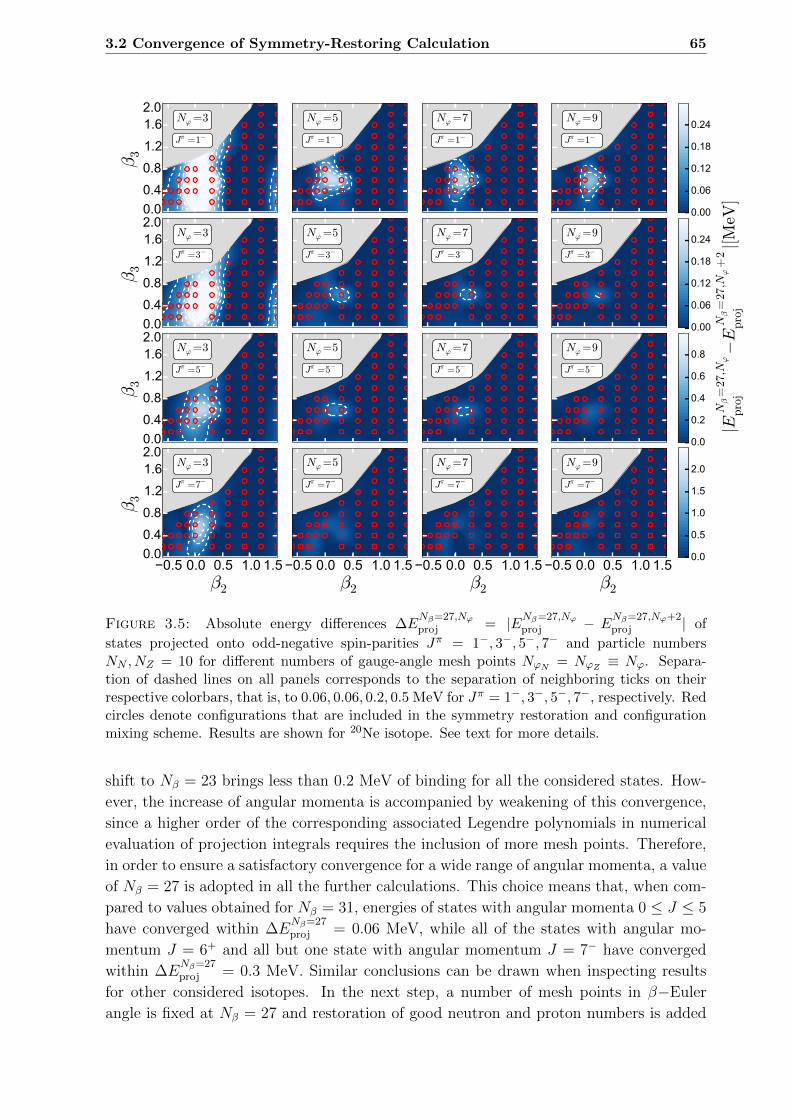
3.2 Convergence of Symmetry-Restoring Calculation 65
−0.5 0.0 0.5 1.0
0.40.81.21.6
β3
0.0
2.0Nϕ=3
Jπ =1−
0.000.250.500.751.001.251.501.752.002.252.50
−0.5 0.0 0.5 1.0
0.4
0.8
1.2
1.6
Nϕ=5
Jπ =1−
−0.5 0.0 0.5 1.0
0.4
0.8
1.2
1.6
Nϕ=7
Jπ =1−
−0.5 0.0 0.5 1.0
0.4
0.8
1.2
1.6
Nϕ=9
Jπ =1−
0.00
0.06
0.12
0.18
0.24
−0.5 0.0 0.5 1.0
0.40.81.21.6
β3
0.0
2.0Nϕ=3
Jπ =3−
−0.5 0.0 0.5 1.0
0.4
0.8
1.2
1.6
Nϕ=5
Jπ =3−
−0.5 0.0 0.5 1.0
0.4
0.8
1.2
1.6
Nϕ=7
Jπ =3−
−0.5 0.0 0.5 1.0
0.4
0.8
1.2
1.6
Nϕ=9
Jπ =3−
0.00
0.06
0.12
0.18
0.24
−0.5 0.0 0.5 1.0
0.40.81.21.6
β3
0.0
2.0Nϕ=3
Jπ =5−
−0.5 0.0 0.5 1.0
0.4
0.8
1.2
1.6
Nϕ=5
Jπ =5−
−0.5 0.0 0.5 1.0
0.4
0.8
1.2
1.6
Nϕ=7
Jπ =5−
−0.5 0.0 0.5 1.0
0.4
0.8
1.2
1.6
Nϕ=9
Jπ =5−
0.0
0.2
0.4
0.6
0.8
−0.5 0.0 0.5 1.0β2
0.40.81.21.6
β3
1.50.0
2.0Nϕ=3
Jπ =7−
−0.5 0.0 0.5 1.0β2
0.4
0.8
1.2
1.6
1.5
Nϕ=5
Jπ =7−
−0.5 0.0 0.5 1.0β2
0.4
0.8
1.2
1.6
1.5
Nϕ=7
Jπ =7−
−0.5 0.0 0.5 1.0β2
0.4
0.8
1.2
1.6
1.5
Nϕ=9
Jπ =7−
0.0
0.5
1.0
1.5
2.0
|ENβ=27,N
ϕ
proj
−ENβ=27,N
ϕ+2
proj
|[MeV
]
Figure 3.5: Absolute energy differences ∆ENβ=27,Nϕproj = |ENβ=27,Nϕ
proj − ENβ=27,Nϕ+2proj | of
states projected onto odd-negative spin-parities Jπ = 1−, 3−, 5−, 7− and particle numbersNN , NZ = 10 for different numbers of gauge-angle mesh points NϕN = NϕZ ≡ Nϕ. Separa-tion of dashed lines on all panels corresponds to the separation of neighboring ticks on theirrespective colorbars, that is, to 0.06, 0.06, 0.2, 0.5 MeV for Jπ = 1−, 3−, 5−, 7−, respectively. Redcircles denote configurations that are included in the symmetry restoration and configurationmixing scheme. Results are shown for 20Ne isotope. See text for more details.
shift to Nβ = 23 brings less than 0.2 MeV of binding for all the considered states. How-
ever, the increase of angular momenta is accompanied by weakening of this convergence,
since a higher order of the corresponding associated Legendre polynomials in numerical
evaluation of projection integrals requires the inclusion of more mesh points. Therefore,
in order to ensure a satisfactory convergence for a wide range of angular momenta, a value
of Nβ = 27 is adopted in all the further calculations. This choice means that, when com-
pared to values obtained for Nβ = 31, energies of states with angular momenta 0 ≤ J ≤ 5
have converged within ∆ENβ=27proj = 0.06 MeV, while all of the states with angular mo-
mentum J = 6+ and all but one state with angular momentum J = 7− have converged
within ∆ENβ=27proj = 0.3 MeV. Similar conclusions can be drawn when inspecting results
for other considered isotopes. In the next step, a number of mesh points in β−Euler
angle is fixed at Nβ = 27 and restoration of good neutron and proton numbers is added

66 Chapter 3 A Computational Interlude
to the states with good angular momenta. In Figure 3.4 we plot the absolute energy dif-
ferences ∆ENβ=27,Nϕproj = |ENβ=27,Nϕ
proj − ENβ=27,Nϕ+2proj | of states projected onto even-positive
spin-parities Jπ = 0+, 2+, 4+, 6+ and particle numbers NN , NZ = 10 for different num-
bers of gauge-angle mesh points NϕN , NϕZ = 3, 5, 7, 9. The corresponding ∆ENβ=27,Nϕproj
values projected onto odd-negative spin-parities Jπ = 1−, 3−, 5−, 7− are shown in Figure
3.5. Starting from the J = 0+ angular momentum, satisfactory convergence is obtained
already for Nϕ = 5 mesh points. However, as in the case of the AMP only, convergence
of the simultaneous AMP and PNP is worsened as the angular momentum is increased.
Therefore, in order to ensure a satisfactory convergence, a value of Nϕ = 9 is adopted in
all the further calculations.
3.2.2 Some Convergence Issues
As previously discussed in Section 2.2.4, a theoretical drawback of all the standard
EDFs, non-relativistic and relativistic alike, is the fact that the Hamiltonian kernel which
they employ does not correspond to the expectation value of a genuine Hamiltonian op-
erator. The unpleasant consequences of this drawback, the appearance of divergences,
finite steps, and/or discontinuities when plotting projected energies as functions of gener-
ating coordinate, have been reported on multiple places [AER01, DSNR07, BDL09]. Even
though these anomalies follow directly from the formal properties of the framework, they
are often not manifested explicitly in practical implementations of the model. The reason
for this is (at least) two-fold: (a) Anomalies are expected to appear only at certain defor-
mations, that is, only for configurations that contain a single-particle level very close to
the Fermi surface. Therefore, a choice of mesh in generating coordinates that is not dense
enough may completely conceal the anomalies. (b) Anomalies are expected to be unveiled
only for very fine discretization meshes of projection integrals. Therefore, discretization
parameters that are typically sufficient to obtain a reasonable convergence may not unveil
the underlying anomalies. In order to demonstrate quantitatively the concrete effect of
this discussion on predictions of our model, in the upper panel of Figure 3.6 we plot the
convergence patterns of energies projected onto angular momentum Jπ = 2+ for all the
states in the RHB basis (this is, of course, equivalent to plotting projected energy as a
function of two generating coordinates). Blue lines denote the case when only AMP is
performed: the dash-dotted line corresponds to difference in projected energies obtained
for Nβ = 27 and Nβ = 71, while the dotted line corresponds to difference in projected
energies obtained with Nβ = 27 and Nβ = 171. Therefore, in addition to calculation per-
formed with the value of discretization parameter that was already demonstrated to yield
satisfactory convergence (Nβ = 27), we performed calculations with two significantly (and
unreasonably) larger values of discretization parameter. Nevertheless, the convergence of
energies of angular-momentum-projected states appears to persist almost perfectly on the
entire β2−β3 plane, save for a barely noticeable dip at around Nstate(β2, β3) = 50. In the
next step, value of AMP discretization parameter was fixed to Nβ = 27 and PNP was
performed with three different values of discretization parameter Nϕ. The corresponding
differences in energies are denoted with red lines: the dash-dotted line corresponds to

3.2 Convergence of Symmetry-Restoring Calculation 67
0 2 4 6 8 10 12 14 16 18 20 22 24 26 28 30 32 34 36 38 40 42 44 46 48 50 52 54 56 58 60−1.6−1.2−0.8−0.40.00.40.81.21.6
∆E
proj [M
eV]
Jπ =2 + Nβ(27)−Nβ(71)
Nϕ(9)−Nϕ(19)
Nβ(27)−Nβ(171)
Nϕ(9)−Nϕ(49)
0 2 4 6 8 10 12 14 16 18 20 22 24 26 28 30 32 34 36 38 40 42 44 46 48 50 52 54 56 58 60
Nstate(β2, β3 > 0)
0.00.10.20.30.40.50.60.70.80.91.0
v2 k
neutrons
protons
Figure 3.6: Upper panel (a): Convergence pattern of energies projected onto angular momen-tum Jπ = 2+ for states Nstate(β2, β3 > 0) in the RHB basis. Blue lines denote the case whenonly AMP is performed: the dash-dotted line corresponds to difference in energies obtained forNβ = 27 and Nβ = 71, while the dotted line corresponds to difference in energies obtained withNβ = 27 and Nβ = 171. Red lines denote the case when both AMP (Nβ = 27) and PNP areperformed: the dash-dotted line corresponds to difference in energies obtained for Nϕ = 9 andNϕ = 19, while the dotted line corresponds to difference in energies obtained with Nϕ = 9 andNϕ = 49. Lower panel (b): Occupation probabilities of single-neutron (circles) and single-proton(triangles) levels of Nstate(β2, β3 > 0) states that are closest to the Fermi surface (v2
k = 0.5).Results are shown for 20Ne isotope. See text for more details.
difference in projected energies obtained with Nϕ = 9 and Nϕ = 19, while the dotted line
corresponds to difference in projected energies obtained with Nϕ = 9 and Nϕ = 49. Once
again, in addition to calculation performed with the value of discretization parameter
that was already demonstrated to yield satisfactory convergence (Nϕ = 9), we performed
calculations with two significantly (and unreasonably) larger values of discretization pa-
rameter. This time, however, we encounter a disturbance in the convergence pattern. In
particular, for Nϕ = 19 small deviations can be seen in the region 6 ≤ Nstate(β2, β3) ≤ 24
that peak at about ∆Eproj ≈ 0.2 MeV for the 14th basis state. To put it into perspective,
let us repeat that a satisfactory convergence of the RHB calculation was proclaimed for
states with ∆ENsh=10RHB ≤ 1 MeV. By further increasing the discretization parameter to
Nϕ = 49, the maximum of deviation switches to 21st basis state and it equals roughly
∆Eproj ≈ 1.5 MeV. As discussed earlier in the manuscript and extensively in the literature
[AER01, DBB+09, BDL09], the origin of these anomalies can be traced back to properties
of the underlying single-particle spectra. In order to examine this claim in more details,
in the lower panel of Fig. 3.6 we plot the occupation probabilities of single-neutron and
single-proton levels of basis states that are closest to the Fermi surface (v2k = 0.5). Com-
paring the two panels, it soon becomes apparent that the ∆Eproj maxima for both red
lines from the upper panel (that is, the 14th and the 21st basis state) indeed correspond
to cases in the lower panel when single-particle states are located very close to the Fermi
surface. Equivalent analyses could be carried out for states with higher values of angular

68 Chapter 3 A Computational Interlude
-164-162-160-158-156-154-152-150
EJ;NZ
;πα
=1
[MeV
]
-158-156-154-152-150-148-146-144
EJ;NZ
;πα
=1
[MeV
]
2 4 6 8 10 12 14 16 18 20 22 24number of norm eigenstates
10-4
10-3
10-2
10-1
100
101
nJ;NZ
;πk
Jπ =0+
Jπ =2+
Jπ =4+
Jπ =6+
2 4 6 8 10 12 14 16 18 20 22 24number of norm eigenstates
10-4
10-3
10-2
10-1
100
101
nJ;NZ
;πk
Jπ =1−
Jπ =3−Jπ =5−
Jπ =7−
Figure 3.7: Upper panel: Excitation energies of collective positive-parity (left) and negative-parity (right) collective states in 20Ne isotope as a function of the number of considered normoverlap eigenstates. Eigenstates are labeled in the decreasing order of eigenvalues. Lower panel:Eigenvalues of the norm overlap for positive-parity (left) and negative-parity (right) collectivestates. See text for more details.
momenta Jπ and for projections with larger values of discretization parameter Nϕ. Both
of these changes are likely to lead to further disturbances of the convergence pattern: the
former one because higher Jπ states have weaker convergence to start with, and the latter
one because larger proportion of the existing pole is likely to be caught by the projection
integral. However, completely spurious-free calculations at the level of implementation
as advanced as the present one are still exceptionally scarce within the non-relativistic
framework [BABH14], and they are yet to be performed within the relativistic framework.
In the meantime, we reiterate that this simple analysis did not reveal any notable issues
concerning AMP calculations, while combined AMP and PNP convergence is yet rather
stable for a reasonable range of discretization parameters.
3.3. Configuration Mixing and Linear Dependencies
Final step of the calculation corresponds to mixing of symmetry-restored RHB config-
urations. The obtained HWG equation is solved by diagonalizing the collective Hamil-
tonian [see Eq. (2.35)] in the basis of natural states [see Eq. (2.37)]. Already a short
inspection of these two equations reveals a potential issue. Namely, if the norm overlap
eigenvalues nJ ;NZ;πk become too small they may cause numerical instabilities when defin-
ing the natural basis and, consequently, when diagonalizing the collective Hamiltonian.
In practice, small values of nJ ;NZ;πk stem from linear dependencies of the initial set of
3.4 Concluding Remarks 69
RHB wave functions |Φ(qi)〉. For this reason, there is no practical gain in including RHB
states that are too close to each other in the space of generating coordinates, since such
choice will only introduce additional linear dependencies to the model. Equivalently, by
choosing the mesh with reasonable ∆β2 and ∆β3 steps one can minimize the influence
of linear dependencies. Nevertheless, they will always persist to a certain level, and they
need to be accounted for. Typically, this is done by inspecting the obtained energies
of collective states as functions of the number of included natural basis states. The so-
called plateau condition then asserts that, after norm overlap eigenstates with smallest
eigenvalues are discarded, these energies should remain rather constant for a wide range
of states [BDF+90]. Therefore, in the upper panel of Figure 3.7 we plot the excitation
energies of collective positive-parity states (left) and negative-parity states (right) in 20Ne
isotope as functions of the number of considered norm overlap eigenstates. We note that
eigenstates with eigenvalues nJ ;NZ;πk < 10−4 were a priori removed from the basis. The
remaining states are labeled in the decreasing order of eigenvalues, that is, the first state
is the one with the largest eigenvalue. The corresponding eigenvalues are additionally
plotted in the lower panel of Fig. 3.7. Inspecting the upper panel of Fig. 3.7, one notices
that energies of the lowest-lying positive-parity states Jπ = 0+, 2+ and negative-parity
states Jπ = 1−, 3−, 5− remain stable for the entire range of norm eigenstates. On the
other hand, for Jπ = 4+, 6+ and Jπ = 7− one first introduces a cutoff in the natural basis
and then adopts the plateau values. Equivalent analysis has been carried out for other
nuclei under consideration and the corresponding plateau values have been adopted.
3.4. Concluding Remarks
To summarize, in this chapter we have discussed computational aspects of our study
that serve as a practical precondition for the successful implementation of the model in
the following chapters. In particular, we have demonstrated that the chosen size of the
axially-symmetric harmonic oscillator basis (Nsh = 10) ensures a satisfactory convergence
of the RHB calculation. Furthermore, we have analyzed in more detail practical issues
related to the restoration of symmetries of the intrinsic states. Values of discretization
parameters Nβ = 27 (for AMP) and Nϕ = 9 (for PNP) were shown to provide a sat-
isfactory convergence of projected energies for angular momenta 0 ≤ J ≤ 7 and for a
wide range of deformations in both the quadrupole and octupole degree of freedom. In
addition, we have briefly discussed the impact of different approximations related to the
form of the effective interaction on predictions of the present model. Our simple analysis
did not reveal any notable issues concerning the AMP calculations, while convergence
of the combined AMP and PNP calculations is rather stable for a reasonable range of
discretization parameters. Finally, we have addressed the impact of linear dependencies
of the initial set of basis functions on final predictions of the collective model. In order
to satify the plateau condition, these linear dependencies are accounted for by inspecting
the obtained collective energies as functions of the size of natural basis and removing the
states related to very small norm eigenvalues. We are now ready to focus on physical
aspects of the study, which will be thoroughly discussed in the following two chapters.


Chapter 4
Quadrupole-Octupole Collectivity
and Clusters in Neon Isotopes
Poets say science takes away from the beauty of the stars - mere globs of gas atoms. Nothing
is ”mere”. I too can see the stars on a desert night, and feel them. But do I see less or more?
Richard Feynman, ”The Feynman Lectures on Physics, Vol. I”
The molecule-like structure of the self-conjugate 20Ne nucleus was first theorized by
the pioneers of nuclear cluster physics already more than 50 years ago [HI68, ITH68].
The two low-lying bands of this isotope, the positive-parity Kπ = 0+ band built upon the
ground state and the negative-parity Kπ = 0− band built upon the first Jπ = 1− state, are
believed to form the inversion doublets and exhibit the equivalent 16O+α structure [HI68,
FHKE+18]. The appearance of clusterized configurations already in the nuclear ground
state is rather exceptional phenomenon in terms of the conventional Ikeda diagrams
[ITH68] which predict the formation of cluster structures as excited states close to the
corresponding α−decay threshold. This almost unique feature of the 20Ne ground state
has attracted significant theoretical attention in the past. Various approaches have been
employed in order to study its low-energy structure, including the angular-momentum-
projected Hartree-Fock model [OYN04], the resonating group method [MKF75], the 5α
generator coordinate method [NYH+75], the antisymmetrized molecular dynamics model
[KEH95, Kim04, TKH04], and the generalized Tohsaki-Horiuchi-Schuck-Ropke wave func-
tion model [ZRX+12]. In addition, reflection-asymmetric equilibrium densities were pre-
dicted within the parity-restored SR-EDF framework, based on both the Gogny [RB11]
and relativistic [EKNV14b] interactions. Another interesting feature of this isotope is the
suggested dissolution of reflection-asymmetric structures at high angular momenta states
by decreasing the equilibrium distance between the two clusters, 16O and α. This is, of
course, unexpected because centrifugal effects should in principle elongate the nucleus.
Recently, a beyond mean-field study of reflection-asymmetric molecular structures and, in
71

72 Chapter 4 Quadrupole-Octupole Collectivity and Clusters in Neon Isotopes
particular, of the antistretching mechanism in 20Ne was performed within the relativistic
MR-EDF framework based on the covariant PC-PK1 functional and the BCS approxima-
tion [ZYL+16]. It has been pointed out that a special deformation-dependent moment of
inertia, governed by the underlying shell structure, could be in part responsible for the
rotation-induced dissolution of cluster structures in the negative-parity states.
Furthermore, in addition to clusters in self-conjugate nuclei, the neutron-rich isotopes
are interesting in the context of excess neutrons playing the role of molecular bonding
between clusterized structures. One such example is the chain of even-even neon isotopes
that can be described as an α + 16O + xn system. The structure of the lightest iso-
tope with such a structure, 22Ne, was previously analyzed with the AMD model [Kim07],
and both the molecular orbital bands and the α + 18O molecular bands has been pre-
dicted. Quadrupole collectivity of heavy neon isotopes close to the neutron drip-line was
previously studied within the EDF framework based on Gogny interaction [RGER03].
Particularly interesting is the case of 24Ne isotope, where a strong shape-coexisting na-
ture of the ground state was predicted [RGER03]. The neutron-rich neon isotopes have
also drawn some attention in the context of nuclear magicity. In particular, a reduction
of the N = 20 spherical shell gap has been experimentally observed in 30Ne isotope, while
a new neutron shell gap was predicted to be formed in 26Ne isotope [SP08].
All things considered, neon isotopic chain, with the formation and dissolution of the
low-lying cluster structures, with the appearance of shape-coexistence phenomenon, and
with the erosion of old and emergence of new magic numbers, represents a truly rich play-
ground for theoretical considerations. In Ref. [MEK+18a] we have studied the structure
of even-even neon isotopes within the relativistic MR-EDF framework. Starting from
a self-consistent RHB calculation of axially-symmetric and reflection-asymmetric defor-
mation energy surfaces, the collective angular-momentum and parity-conserving states
were built using projection and configuration mixing techniques. In the present work, we
are further extending that framework by including the projection of intrinsic states onto
good neutron and proton numbers. Following the strategy of Ref. [MEK+18a], the fully
symmetry-restoring framework is employed in a systematic study of quadrupole-octupole
collectivity and cluster structures in neon isotopes. The content and the form of the
chapter will therefore largely rely on the analysis carried out in Ref. [MEK+18a]. In
Section 4.1, we will study the ground-state properties of neon isotopic chain, including
binding energies, charge radii, and two-neutron separation energies. Furthermore, we will
demonstrate the effect of symmetry restoration and configuration mixing on a structure
of the ground state and analyze the obtained wave functions in some more detail. In
Section 4.2, we will study the low-lying systematics of the neon isotopic chain, including
potential energy surfaces projected onto various angular momenta, excitation energies
of the low-lying collective states, as well as the transition strengths between them. De-
tailed spectroscopy of 22,24Ne and 32,34Ne isotopes will additionally be analyzed. Finally,
in Section 4.3 we will focus more attention on the particularly interesting case of the
self-conjugate 20Ne isotope. The obtained spectroscopic properties will be thoroughly
compared to the available experimental data and to the predictions of other theoretical
models. In addition, cluster components of collective states in the intrinsic frame will be
analyzed.

4.1 Ground-State Properties of Neon Isotopes 73
−0.8 −0.4 0.0 0.4 0.8 1.2
0.25
0.50
0.75
1.00
1.25
β3
0.00
1.5020 Ne
−0.8 −0.4 0.0 0.4 0.8 1.2
0.25
0.50
0.75
1.00
1.25
22 Ne
−0.8 −0.4 0.0 0.4 0.8 1.2
0.25
0.50
0.75
1.00
1.25
24 Ne
−0.8 −0.4 0.0 0.4 0.8 1.2
0.25
0.50
0.75
1.00
1.25
26 Ne
−0.8 −0.4 0.0 0.4 0.8 1.2β2
0.25
0.50
0.75
1.00
1.25
β3
1.60.00
1.5028 Ne
−0.8 −0.4 0.0 0.4 0.8 1.2β2
0.25
0.50
0.75
1.00
1.25
1.6
30 Ne
−0.8 −0.4 0.0 0.4 0.8 1.2β2
0.25
0.50
0.75
1.00
1.25
1.6
32 Ne
−0.8 −0.4 0.0 0.4 0.8 1.2β2
0.25
0.50
0.75
1.00
1.25
1.6
34 Ne
0
5
10
15
20
ERHB [M
eV]
Figure 4.1: Self-consistent RHB binding energies of even-even 20−34Ne isotopes, in the β2−β3
plane. For each nucleus, energies are normalized with respect to the energy of the correspondingabsolute minimum. Dashed contours are separated by 2 MeV.
4.1. Ground-State Properties of Neon Isotopes
4.1.1 The Mean-Field Analysis
Our analysis of the ground-state properties of even-even neon isotopes starts with the
self-consistent RHB calculation. The RHB equations were solved in the configurational
space of axially-symmetric harmonic oscillator, by expanding the large and the small
component of nuclear spinors in the corresponding bases with Nsh = 10 and Nsh = 11, re-
spectively. These calculations cover a wide range of deformations in both the quadrupole
and octupole direction, β2 ∈ [−0.6, 1.5] and β3 ∈ [−2.0, 2.0], with steps in the oblate,
prolate, and octupole direction being ∆β2 = 0.15, ∆β2 = 0.3, and ∆β3 = 0.2, respec-
tively. The obtained binding energies for the entire isotopic chain are shown in Figure 4.1.
For each isotope, energies have been normalized with respect to the energy of the corre-
sponding absolute minimum. These minima are found at reflection-symmetric (β3 = 0)
configurations along the entire isotopic chain, and the corresponding quadrupole defor-
mation parameters, binding energies, and charge radii are listed in Table 4.1. Two of the
lightest isotopes considered, 20Ne and 22Ne, are prolate-deformed nuclei with equilibrium
quadrupole deformations β2 ≈ 0.5. By adding two more neutrons, a nearly-degenerate
oblate-deformed minimum at β2 = −0.27 and prolate-deformed minimum at β2 = 0.29 are
developed in 24Ne. Further addition of neutrons leads to development of nearly-spherical
minima in 26Ne and 28Ne isotopes, and a spherical equilibrium in 30Ne isotope due to
the N = 20 neutron shell closure. Moving further away from the magic number, the
neutron-rich isotopes 32Ne and 34Ne display prolate minima with deformations β2 = 0.31

74 Chapter 4 Quadrupole-Octupole Collectivity and Clusters in Neon Isotopes
Table 4.1: Self-consistent RHB values of the axial quadrupole deformation parameters β2 inground states of 20−34Ne isotopes. Axial octupole deformation parameters β3 vanish in groundstates of all isotopes. In addition, equilibrium binding energies (second row) and charge radii(fourth row) are given. The corresponding relative errors with respect to the experimental data,
Rcalc.-exp.err = (Ecalc.
B − Eexp.B )/|Eexp.
B |, on binding energies [WAK+17] and charge radii [AM13],are given in the third and the fifth row, respectively.
20Ne 22Ne 24Ne 26Ne 28Ne 30Ne 32Ne 34Ne
β2 0.51 0.50 −0.25 −0.04 −0.05 0.00 0.31 0.43
EB [MeV] −157.89 −177.24 −191.03 −202.95 −211.48 −218.68 −218.95 −220.23
Rcalc.-exp.err [%] 1.6 0.3 0.4 −0.6 −2.2 −3.6 −2.6 −3.0
Rch [fm] 3.00 2.99 2.94 2.93 2.98 3.02 3.09 3.14
Rcalc.-exp.err [%] −0.2 1.3 1.4 0.2 0.5 − − −
and β2 = 0.43, respectively.
Calculated binding energies of equilibrium configurations are listed in the second row
of Tab. 4.1 and the corresponding relative errors in comparison with the experimental
data [WAK+17], Rcalc.-exp.err = (Ecalc.
B − Eexp.B )/|Eexp.
B |, are listed in the third row. Overall
agreement for lighter isotopes is quite good, while our calculation tends to overestimate
binding energy of neutron-rich isotopes. Similar behavior was already observed in the rel-
ativistic HFB calculations based on the DD-ME2 functional [EKAV11]. In addition, the
large-scale calculations based on the Gogny D1S force reported a systematic drift towards
theoretical overbinding in neutron-rich isotopes [HG07]. This anomaly was linked to the
imprecise treatment of energy dependence in the neutron matter during fitting procedure
and it was fixed in later parameterizations [CGH08, GHGP09]. We note that the DD-
PC1 functional was fitted exclusively to data on finite nuclei and that the overbinding
of closed-shell systems due to a relatively low effective nucleon mass was noticed already
in the very first application [NVR08]. Therefore, it is expected that the largest devi-
ation in Tab. 4.1 is found in the spherical 30Ne isotope. Moreover, the ground-state
quadrupole deformation of 30Ne is, in fact, experimentally well-established [SP08] and
this overbinding can, at least partially, be attributed to the fact that the obtained spheri-
cal state includes the abnormally large amount of pairing correlations. These correlations
increase the total binding energy of a nucleus and would normally be absent from the
well-deformed state. Generally, it is well known that the choice of the pairing force has a
significant impact on the topology of potential energy surfaces. In particular, larger pair-
ing strength drives energy surfaces towards spherical shapes [AAR16], which has a direct
and important influence on heights of fission barriers and spontaneous fission half-lives in
heavy and superheavy nuclei [KALR10, RGR14]. In this context, one should note that
the parameters of pairing force used in this study were originally adjusted to reproduce
the pairing gap at the Fermi surface in symmetric nuclear matter as calculated with the
Gogny D1S force [TMR09a]. Therefore, there is no guarantee that the same parameters
will be optimal for calculations in finite nuclei over the entire nuclide chart. In practice,
one could fine tune the pairing strength in order to better reproduce experimental binding

4.1 Ground-State Properties of Neon Isotopes 75
(a) (b)
Figure 4.2: Nucleon densities (in fm−3) of 20Ne in the x − z plane of the intrinsic frame ofreference. Left panel (a): Density corresponding to the absolute minimum (β2, β3) = (0.51, 0.0)of the self-consistent RHB energy surface [see Fig. 4.1]. Right panel (b): Density correspondingto the absolute minimum (β2, β3) = (0.45, 0.40) of the symmetry-restored Jπ = 0+ energysurface [see Fig. 4.3].
energies or available empirical pairing gaps in finite nuclei. However, for the sake of stay-
ing true to the principle of globality, we choose to stick to the exactly same parameters
of the pairing interaction over the entire isotopic chain.
Calculated charge radii of equilibrium configuration are given in the fourth row of Table
4.1. They compare rather favorably with the experimental data [AM13], as well as with
the relativistic HFB calculations based on the DD-ME2 functional [EKAV11]. The 20Ne
ground state is associated with a large quadrupole deformation, which gives rise to the
intrinsically-deformed charge distribution and, consequently, large charge radius. On the
other hand, the smallest charge radius is found in 24Ne isotope, due to the d5/2 subshell
closure. Further addition of neutrons leads to the enhancement of charge radii in heavier
isotopes. However, the charge radius of 20Ne is first exceeded only in 30Ne, an isotope
with twice as large number of neutrons. The large quadrupole deformation of the 20Ne
ground state is mirrored in its deformed intrinsic density distribution, which is plotted in
the left panel of Figure 4.2.
4.1.2 The Effect of Collective Correlations
The mean-field approach is characterized by breaking of various symmetries that even-
tually need to be recovered. Restoration of angular momentum, particle number, and

76 Chapter 4 Quadrupole-Octupole Collectivity and Clusters in Neon Isotopes
−0.8 −0.4 0.0 0.4 0.8 1.2
0.25
0.50
0.75
1.00
1.25
β3
0.00
1.5020 NeJπ =0+
−0.8 −0.4 0.0 0.4 0.8 1.2
0.25
0.50
0.75
1.00
1.25
22 NeJπ =0+
−0.8 −0.4 0.0 0.4 0.8 1.2
0.25
0.50
0.75
1.00
1.25
24 NeJπ =0+
−0.8 −0.4 0.0 0.4 0.8 1.2
0.25
0.50
0.75
1.00
1.25
26 NeJπ =0+
−0.8 −0.4 0.0 0.4 0.8 1.2β2
0.25
0.50
0.75
1.00
1.25
β3
1.60.00
1.5028 NeJπ =0+
−0.8 −0.4 0.0 0.4 0.8 1.2β2
0.25
0.50
0.75
1.00
1.25
1.6
30 NeJπ =0+
−0.8 −0.4 0.0 0.4 0.8 1.2β2
0.25
0.50
0.75
1.00
1.25
1.6
32 NeJπ =0+
−0.8 −0.4 0.0 0.4 0.8 1.2β2
0.25
0.50
0.75
1.00
1.25
1.6
34 NeJπ =0+
0
5
10
15
20
EJπ
proj [
MeV
]
Figure 4.3: Angular momentum-, particle number-, and parity-projected energy surfaces ofeven-even 20−34Ne isotopes, for spin and parity Jπ = 0+ in the β2 − β3 plane. For eachnucleus, energies are normalized with respect to the binding energy of the corresponding absoluteminimum. Dashed contours are separated by 2 MeV.
parity symmetry were simultaneously performed within our study, using the tools de-
scribed in previous chapters. Discretization parameters of the corresponding integrals,
that is Nβ = 27 for AMP and Nϕ = 9 for PNP, were verified to ensure satisfactory con-
vergence for all values of angular momenta 0 ≤ J ≤ 7 and a broad range of quadrupole
and octupole deformations [for more details, see Chapter 3]. In order to demonstrate
the influence of symmetry restoration on topology of the ground-state potential energy
surfaces, in Figure 4.3 we show the angular-momentum, particle-number, and parity-
projected potential energy surfaces of ground states (Jπ = 0+) of 20−34Ne isotopes in
β2 − β3 plane. A prominent feature in Fig. 4.3 is the fact that parity projection shifts
the position of all the minima towards reflection-asymmetric (β3 6= 0) configurations.
Angular momentum and particle number projections additionally modify the topography
of mean-field energy maps by lowering deformed configurations, thereby forming local
oblate-deformed minima for all isotopes. In particular, an absolute minimum for the20Ne isotope is found at the octupole-deformed (β2 = 0.45, β3 = 0.4) configuration. The
characteristic pear-like density distribution which corresponds to the equivalent (β2, β3)
configuration in the intrinsic frame1 is plotted in the right panel of Fig. 4.2.
However, the obtained energy surfaces are rather soft in both the β2 and β3 directions,
indicating that configuration mixing calculations will play a crucial role for a quantitative
description of the structure of neon isotopes. Solving the corresponding HWG equation
gives us an access to the correlated ground states, as well as to the structure of the excited
states. Here, one should recall that parameters of the effective interaction [NVR08] have
1Of course, density distribution of the symmetry-restored Jπ = 0+ state in the laboratory frame forany (β2, β3) combination would be spherically symmetric.
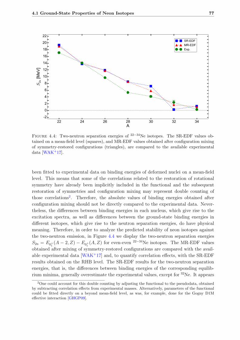
4.1 Ground-State Properties of Neon Isotopes 77
22 24 26 28 30 32 34A
-2
0
2
4
6
8
10
12
14
16
18
20
22S
2n [M
eV]
SR-EDFMR-EDFExp.
Figure 4.4: Two-neutron separation energies of 22−34Ne isotopes. The SR-EDF values ob-tained on a mean-field level (squares), and MR-EDF values obtained after configuration mixingof symmetry-restored configurations (triangles), are compared to the available experimentaldata [WAK+17].
been fitted to experimental data on binding energies of deformed nuclei on a mean-field
level. This means that some of the correlations related to the restoration of rotational
symmetry have already been implicitly included in the functional and the subsequent
restoration of symmetries and configuration mixing may represent double counting of
those correlations2. Therefore, the absolute values of binding energies obtained after
configuration mixing should not be directly compared to the experimental data. Never-
theless, the differences between binding energies in each nucleus, which give rise to the
excitation spectra, as well as differences between the ground-state binding energies in
different isotopes, which give rise to the neutron separation energies, do have physical
meaning. Therefore, in order to analyze the predicted stability of neon isotopes against
the two-neutron emission, in Figure 4.4 we display the two-neutron separation energies
S2n = E0+1(A − 2, Z) − E0+1
(A,Z) for even-even 22−34Ne isotopes. The MR-EDF values
obtained after mixing of symmetry-restored configurations are compared with the avail-
able experimental data [WAK+17] and, to quantify correlation effects, with the SR-EDF
results obtained on the RHB level. The SR-EDF results for the two-neutron separation
energies, that is, the differences between binding energies of the corresponding equilib-
rium minima, generally overestimate the experimental values, except for 32Ne. It appears
2One could account for this double counting by adjusting the functional to the pseudodata, obtainedby subtracting correlation effects from experimental masses. Alternatively, parameters of the functionalcould be fitted directly on a beyond mean-field level, as was, for example, done for the Gogny D1Meffective interaction [GHGP09].

78 Chapter 4 Quadrupole-Octupole Collectivity and Clusters in Neon Isotopes
−0.6 −0.3 0.0 0.3 0.6 0.9 1.2 1.5
0.25
0.50
0.75
1.00
1.25
β3
0.00
1.5020NeJπ =0+
0.01 0.02 0.03|g(β2 ,β3 )|2
0.00 0.04
−0.6 −0.3 0.0 0.3 0.6 0.9 1.2 1.5
0.25
0.50
0.75
1.00
1.25
1.50
22NeJπ =0+
0.015 0.030 0.045|g(β2 ,β3 )|2
0.00 0.06
−0.6 −0.3 0.0 0.3 0.6 0.9 1.2 1.5
0.25
0.50
0.75
1.00
1.25
1.50
24NeJπ =0+
0.01 0.02 0.03|g(β2 ,β3 )|2
0.00 0.04
−0.6 −0.3 0.0 0.3 0.6 0.9 1.2 1.5
0.25
0.50
0.75
1.00
1.25
1.50
26NeJπ =0+
0.015 0.030 0.045|g(β2 ,β3 )|2
0.00 0.06
−0.6 −0.3 0.0 0.3 0.6 0.9 1.2β2
0.25
0.50
0.75
1.00
1.25
β3
1.50.00
1.5028NeJπ =0+
0.015 0.030 0.045|g(β2 ,β3 )|2
0.00 0.06
−0.6 −0.3 0.0 0.3 0.6 0.9 1.2β2
0.25
0.50
0.75
1.00
1.25
1.50
1.5
30NeJπ =0+
0.02 0.04 0.06|g(β2 ,β3 )|2
0.00 0.08
−0.6 −0.3 0.0 0.3 0.6 0.9 1.2β2
0.25
0.50
0.75
1.00
1.25
1.50
1.5
32NeJπ =0+
0.015 0.030 0.045|g(β2 ,β3 )|2
0.00 0.06
−0.6 −0.3 0.0 0.3 0.6 0.9 1.2β2
0.25
0.50
0.75
1.00
1.25
1.50
1.5
34NeJπ =0+
0.02 0.04 0.06|g(β2 ,β3 )|2
0.00 0.08
Figure 4.5: Amplitudes of collective wave functions squared |g(β2, β3)|2 of the ground statesof 20−34Ne isotopes. Dashed contours in the β2 − β3 plane successively denote a 10% decreasestarting from the largest value of the amplitude.
that for A < 30 configuration mixing does not produce a significant impact on the calcu-
lated two-neutron separation energies. Closer to the dripline, however, one notices that
the inclusion of collective correlations through symmetry restoration and configuration
mixing starts to play much more important role, shifting calculated values closer to the
experimental ones. In addition, we have verified that 34Ne is indeed the last stable neon
isotope, since both the two-neutron and the four-neutron separation energies for 36Ne
are calculated to be negative. A similar improvement of the predicted two-neutron sepa-
ration energies for neon isotopes was also obtained in the angular-momentum-projected
configuration mixing study based on the Gogny D1S interaction [RGER03]. However, the
calculated S2n value for 34Ne reported therein was slightly negative, that is, this isotope
was predicted to be unstable against the two-neutron emission.
Even though the ground-state spectroscopic quadrupole moments vanish identically in
even-even nuclei, it is instructive to calculate expectation values of quadrupole deforma-
tion parameters in correlated ground states. These values can be obtained by averaging
the deformation parameter β2 over the entire β2 − β3 plane, with the wave functions of
each collective state Jπα playing the role of corresponding weights [see Eq. (2.40)]. In Fig-
ure 4.5 we display the amplitudes squared of the ground-state collective wave functions
for 20−34Ne. As noted before, this quantity is not an observable, but still it provides a
useful insight into the structure of correlated ground states. In contrast to the mean-field
RHB equilibrium minimum which corresponds to a single configuration in the (β2, β3)
plane, the amplitude of the ground state collective wave function manifests the degree
of shape fluctuations in both quadrupole and octupole directions. In the left panel of
Figure 4.6 we plot the MR-EDF average β2 deformation values for 20−34Ne isotopes in

4.1 Ground-State Properties of Neon Isotopes 79
20 22 24 26 28 30 32 34A
-0.4 -0.3 -0.2-0.10.00.10.20.30.40.50.60.70.8
β2
(76%)
(72%)
(61%)
(58%)
(67%)(65%)
(69%)
(73%)
(24%) (28%)
(39%)
(42%) (33%)
(35%)(31%) (27%)
(a) (b)
20 22 24 26 28 30 32 34A
0.0
0.1
0.2
0.3
0.4
0.5
0.6
|β3|
SR-EDFMR-EDF totalMR-EDF prolateMR-EDF oblate
Figure 4.6: Deformation parameters β2 (left panel (a)) and |β3| (right panel (b)) of 20−34Neisotopes that correspond to self-consistent minima on the SR-EDF level, in comparison withthe MR-EDF values of the corresponding correlated ground states. The deformations obtainedby averaging over only prolate (triangle left) and only oblate (triangle right) configurations, aswell as their respective contributions to the total collective wave function, are also shown.
comparison to deformations that correspond to the self-consistent minima on the SR-
EDF level. Since the contributions of oblate configurations to the total collective wave
functions are larger than 20% over the entire isotopic chain, we additionally display the
β2 deformations obtained by averaging over only prolate (left triangle) and only oblate
(right triangle) configurations. In parentheses, we include the respective contributions
to the total collective wave function from both prolate and oblate configurations. One
notices that oblate configurations give a significant contribution for all isotopes, and this
contribution is more pronounced in 24−32Ne. The nucleus 24Ne, which exhibits nearly de-
generate oblate and prolate minima on the mean-field level, preserves this structure even
after symmetry restoration and configuration mixing. In particular, dominant component
of the correlated ground state is prolate-deformed and peaks at β2 ≈ 0.35, but nearly
40% of the collective wave function spreads over the oblate side and peaks at β2 ≈ 0.3. A
similar behavior is also found in the 26Ne isotope. The semimagic nucleus 30Ne is found
to be very weakly prolate-deformed, in contrast to the large ground-state quadrupole
deformation deduced from the experiment [SP08]. By removing two neutrons, the nearly
spherical structure of the ground state appears to be preserved in 28Ne. The addition of
two neutrons, however, leads to the formation of a barrier at the spherical configuration
of 32Ne. The resulting collective wave function resembles the shape-coexisting structure,
even though the prolate component is significantly more pronounced. In the right panel of
Fig. 4.6 we plot the corresponding values of the octupole deformation parameter. Since
〈β3〉 vanishes identically for all collective states with good parity, we plot instead the
average values of the corresponding modulus [see Eq. (2.41)]. The 〈|β3|〉 values quantify
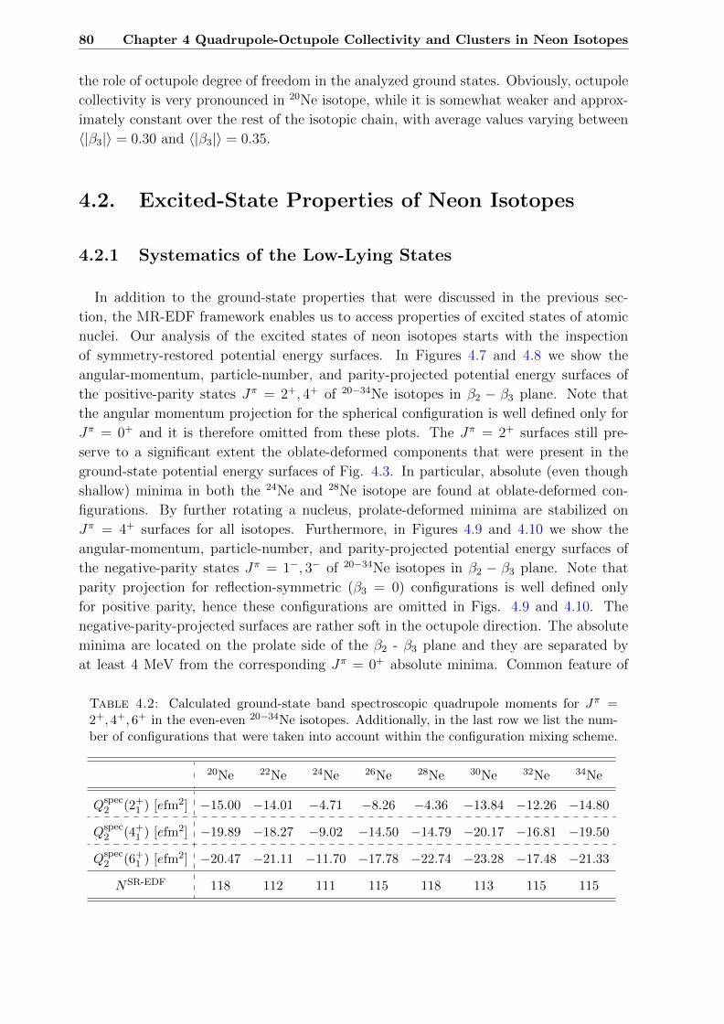
80 Chapter 4 Quadrupole-Octupole Collectivity and Clusters in Neon Isotopes
the role of octupole degree of freedom in the analyzed ground states. Obviously, octupole
collectivity is very pronounced in 20Ne isotope, while it is somewhat weaker and approx-
imately constant over the rest of the isotopic chain, with average values varying between
〈|β3|〉 = 0.30 and 〈|β3|〉 = 0.35.
4.2. Excited-State Properties of Neon Isotopes
4.2.1 Systematics of the Low-Lying States
In addition to the ground-state properties that were discussed in the previous sec-
tion, the MR-EDF framework enables us to access properties of excited states of atomic
nuclei. Our analysis of the excited states of neon isotopes starts with the inspection
of symmetry-restored potential energy surfaces. In Figures 4.7 and 4.8 we show the
angular-momentum, particle-number, and parity-projected potential energy surfaces of
the positive-parity states Jπ = 2+, 4+ of 20−34Ne isotopes in β2 − β3 plane. Note that
the angular momentum projection for the spherical configuration is well defined only for
Jπ = 0+ and it is therefore omitted from these plots. The Jπ = 2+ surfaces still pre-
serve to a significant extent the oblate-deformed components that were present in the
ground-state potential energy surfaces of Fig. 4.3. In particular, absolute (even though
shallow) minima in both the 24Ne and 28Ne isotope are found at oblate-deformed con-
figurations. By further rotating a nucleus, prolate-deformed minima are stabilized on
Jπ = 4+ surfaces for all isotopes. Furthermore, in Figures 4.9 and 4.10 we show the
angular-momentum, particle-number, and parity-projected potential energy surfaces of
the negative-parity states Jπ = 1−, 3− of 20−34Ne isotopes in β2 − β3 plane. Note that
parity projection for reflection-symmetric (β3 = 0) configurations is well defined only
for positive parity, hence these configurations are omitted in Figs. 4.9 and 4.10. The
negative-parity-projected surfaces are rather soft in the octupole direction. The absolute
minima are located on the prolate side of the β2 - β3 plane and they are separated by
at least 4 MeV from the corresponding Jπ = 0+ absolute minima. Common feature of
Table 4.2: Calculated ground-state band spectroscopic quadrupole moments for Jπ =2+, 4+, 6+ in the even-even 20−34Ne isotopes. Additionally, in the last row we list the num-ber of configurations that were taken into account within the configuration mixing scheme.
20Ne 22Ne 24Ne 26Ne 28Ne 30Ne 32Ne 34Ne
Qspec2 (2+
1 ) [efm2] −15.00 −14.01 −4.71 −8.26 −4.36 −13.84 −12.26 −14.80
Qspec2 (4+
1 ) [efm2] −19.89 −18.27 −9.02 −14.50 −14.79 −20.17 −16.81 −19.50
Qspec2 (6+
1 ) [efm2] −20.47 −21.11 −11.70 −17.78 −22.74 −23.28 −17.48 −21.33
NSR-EDF 118 112 111 115 118 113 115 115

4.2 Excited-State Properties of Neon Isotopes 81
−0.8 −0.4 0.0 0.4 0.8 1.2
0.25
0.50
0.75
1.00
1.25
β3
0.00
1.5020 NeJπ =2+
−0.8 −0.4 0.0 0.4 0.8 1.2
0.25
0.50
0.75
1.00
1.25
22 NeJπ =2+
−0.8 −0.4 0.0 0.4 0.8 1.2
0.25
0.50
0.75
1.00
1.25
24 NeJπ =2+
−0.8 −0.4 0.0 0.4 0.8 1.2
0.25
0.50
0.75
1.00
1.25
26 NeJπ =2+
−0.8 −0.4 0.0 0.4 0.8 1.2β2
0.25
0.50
0.75
1.00
1.25
β3
1.60.00
1.5028 NeJπ =2+
−0.8 −0.4 0.0 0.4 0.8 1.2β2
0.25
0.50
0.75
1.00
1.25
1.6
30 NeJπ =2+
−0.8 −0.4 0.0 0.4 0.8 1.2β2
0.25
0.50
0.75
1.00
1.25
1.6
32 NeJπ =2+
−0.8 −0.4 0.0 0.4 0.8 1.2β2
0.25
0.50
0.75
1.00
1.25
1.6
34 NeJπ =2+
0
5
10
15
20
EJπ
proj [
MeV
]
Figure 4.7: Angular momentum-, particle number-, and parity-projected energy surfaces ofeven-even 20−34Ne isotopes, for spin and parity Jπ = 2+ in the β2−β3 plane. For each nucleus,energies are normalized with respect to the binding energy of the corresponding Jπ = 0+
absolute minimum. Dashed contours are separated by 2 MeV.
all projected energy maps is that restoration of symmetries significantly modifies the ini-
tial topology of each map, indicating that configuration mixing calculations will play a
crucial role for a quantitative description of the structure of neon isotopes. In Table 4.2
we therefore list the number of configurations NSR-EDF that were taken into account for
each isotope within the configuration mixing scheme. As explained earlier, a set of RHB
states was initially generated on a discretized mesh in the β2 − β3 plane. Configurations
−0.8 −0.4 0.0 0.4 0.8 1.2
0.25
0.50
0.75
1.00
1.25
β3
0.00
1.5020 NeJπ =4+
−0.8 −0.4 0.0 0.4 0.8 1.2
0.25
0.50
0.75
1.00
1.25
22 NeJπ =4+
−0.8 −0.4 0.0 0.4 0.8 1.2
0.25
0.50
0.75
1.00
1.25
24 NeJπ =4+
−0.8 −0.4 0.0 0.4 0.8 1.2
0.25
0.50
0.75
1.00
1.25
26 NeJπ =4+
−0.8 −0.4 0.0 0.4 0.8 1.2β2
0.25
0.50
0.75
1.00
1.25
β3
1.60.00
1.5028 NeJπ =4+
−0.8 −0.4 0.0 0.4 0.8 1.2β2
0.25
0.50
0.75
1.00
1.25
1.6
30 NeJπ =4+
−0.8 −0.4 0.0 0.4 0.8 1.2β2
0.25
0.50
0.75
1.00
1.25
1.6
32 NeJπ =4+
−0.8 −0.4 0.0 0.4 0.8 1.2β2
0.25
0.50
0.75
1.00
1.25
1.6
34 NeJπ =4+
0
5
10
15
20
EJπ
proj [
MeV
]
Figure 4.8: Same as in the caption to Figure 4.7, but for spin and parity Jπ = 4+.

82 Chapter 4 Quadrupole-Octupole Collectivity and Clusters in Neon Isotopes
−0.8 −0.4 0.0 0.4 0.8 1.2
0.25
0.50
0.75
1.00
1.25
β3
0.00
1.5020 NeJπ =1−
−0.8 −0.4 0.0 0.4 0.8 1.2
0.25
0.50
0.75
1.00
1.25
22 NeJπ =1−
−0.8 −0.4 0.0 0.4 0.8 1.2
0.25
0.50
0.75
1.00
1.25
24 NeJπ =1−
−0.8 −0.4 0.0 0.4 0.8 1.2
0.25
0.50
0.75
1.00
1.25
26 NeJπ =1−
−0.8 −0.4 0.0 0.4 0.8 1.2β2
0.25
0.50
0.75
1.00
1.25
β3
1.60.00
1.5028 NeJπ =1−
−0.8 −0.4 0.0 0.4 0.8 1.2β2
0.25
0.50
0.75
1.00
1.25
1.6
30 NeJπ =1−
−0.8 −0.4 0.0 0.4 0.8 1.2β2
0.25
0.50
0.75
1.00
1.25
1.6
32 NeJπ =1−
−0.8 −0.4 0.0 0.4 0.8 1.2β2
0.25
0.50
0.75
1.00
1.25
1.6
34 NeJπ =1−
0
5
10
15
20
EJπ
proj [
MeV
]
Figure 4.9: Angular momentum-, particle number-, and parity-projected energy surfaces ofeven-even 20−34Ne isotopes, for spin and parity Jπ = 1− in the β2−β3 plane. For each nucleus,energies are normalized with respect to the binding energy of the corresponding Jπ = 0+
absolute minimum. Dashed contours are separated by 2 MeV.
with binding energies that are much higher than energy of the equilibrium configuration
(roughly 20 MeV and above) are eliminated from the basis. In this way, one keeps the
number of configurations that are being mixed between 110 and 120. Of course, the ex-
clusion of such high-energy states does not influence the predictive power of a model that
ultimately aims to describe the low-lying nuclear structure. The remaining states are
projected onto good quantum numbers and further mixed within the GCM framework.
−0.8 −0.4 0.0 0.4 0.8 1.2
0.25
0.50
0.75
1.00
1.25
β3
0.00
1.5020 NeJπ =3−
−0.8 −0.4 0.0 0.4 0.8 1.2
0.25
0.50
0.75
1.00
1.25
22 NeJπ =3−
−0.8 −0.4 0.0 0.4 0.8 1.2
0.25
0.50
0.75
1.00
1.25
24 NeJπ =3−
−0.8 −0.4 0.0 0.4 0.8 1.2
0.25
0.50
0.75
1.00
1.25
26 NeJπ =3−
−0.8 −0.4 0.0 0.4 0.8 1.2β2
0.25
0.50
0.75
1.00
1.25
β3
1.60.00
1.5028 NeJπ =3−
−0.8 −0.4 0.0 0.4 0.8 1.2β2
0.25
0.50
0.75
1.00
1.25
1.6
30 NeJπ =3−
−0.8 −0.4 0.0 0.4 0.8 1.2β2
0.25
0.50
0.75
1.00
1.25
1.6
32 NeJπ =3−
−0.8 −0.4 0.0 0.4 0.8 1.2β2
0.25
0.50
0.75
1.00
1.25
1.6
34 NeJπ =3−
0
5
10
15
20E
Jπ
proj [
MeV
]
Figure 4.10: Same as in the caption to Figure 4.9, but for spin and parity Jπ = 3−.

4.2 Excited-State Properties of Neon Isotopes 83
20 22 24 26 28 30 32 34A
0.0
1.0
2.0
3.0
4.0
5.0
6.0
7.0
8.0
9.0
10.0
Ex [M
eV]
(a) (b)
2+1 MR-EDF
2+1 Exp.
4+1 MR-EDF
4+1 Exp.
20 22 24 26 28 30 32 34A
051015202530354045505560657075
B(E
2;2
+ 1→
0+ 1
) [e2
fm4
]
MR-EDFExp.
Figure 4.11: Calculated excitation energies of the 2+1 and 4+
1 states [left panel (a)] and thetransition strengths B(E2; 2+
1 → 0+1 ) [right panel(b)] in even-even 20−34Ne isotopes, compared
with the available experimental data [NNNDC, PBSH16].
The obtained excitation energies of the 2+1 and 4+
1 states in 20−34Ne isotopes are plotted in
the left panel of Fig. 4.11 and compared to the available experimental data. Predictions
of our model for lighter isotopes 20−24Ne are in rather good agreement with data. How-
ever, when approaching the N = 20 neutron shell the theoretical results begin to diverge
from experiment, and this is especially pronounced in the 30Ne isotope. This discrepancy
originates from the fact that the DD-PC1 functional predicts the N = 20 neutron shell
closure even for the very neutron-rich isotopes. On the other hand, the breakdown of the
N = 20 neutron magic number is experimentally a well-established phenomenon [SP08],
leading to the large quadrupole deformation in the ground state of 30Ne isotope. We note
that a similar issue occurred in a previous study of 32Mg based on the relativistic func-
tional PC-F1 [NVR06a], as well as in some calculations based on non-relativistic EDFs,
e.g., the SLy4 effective interaction [HBC+00]. In addition, the present study is restricted
to axial shapes, whereas in some of the heavier isotopes additional degrees of freedom,
such as triaxial, could play an important role.
The calculated electric transition rates from these 2+1 states to the corresponding
ground states are displayed in the right panel of Fig. 4.11 and compared with the avail-
able data. Theoretical results reproduce the experimental values rather well over the
entire isotopic chain. The only exception is 30Ne isotope where, because of the predicted
N = 20 neutron shell closure, we obtain the B(E2; 2+1 → 0+
1 ) value that is much smaller
than the corresponding experimental value. Furthermore, in Table 4.2 we list the calcu-
lated ground-state band spectroscopic quadrupole moments for neon isotopic chain. In
comparison to the previously reported values that were calculated without the particle
number projection [MEK+18a], the newly-obtained values of Qspec2 (2+
1 ) are systematically
reduced in all isotopes. This phenomenon can be understood as a consequence of the fact

84 Chapter 4 Quadrupole-Octupole Collectivity and Clusters in Neon Isotopes
0
2
4
6
8
10
12
14
16
18
20
EX
[M
eV]
0+
4+
6+
1-
2+
3-
5-
7-
55
79
87
22Ne
132
144
135
90
130
K=01
+K=0
1
-0
+
2+
4+
6+
153
1-
3-
5-
7-
130
37
58
68
112
K=01
+K=0
1
-
MR-EDF MR-EDF
182
24Ne
49105
108
0+
4+
6+
1-
2+
3-
5-
7-
39
66
71
32Ne
99
114
121
93
64
K=01
+K=0
1
-0
+2
+
4+
6+
142
1-
3-
5-
7-
138
54
86
94
121
K=01
+K=0
1
-
MR-EDF MR-EDF
107
34Ne
7113
8
124
Figure 4.12: Calculated low-energy spectra of 22,24Ne (left panel) and 32,34Ne (right panel).The E2 reduced transition strengths within the bands (red color, in e2fm4) and E3 transitionstrengths between the bands (blue color, in e2fm6) are also shown.
that PNP additionally lowers energies of the oblate-deformed configurations, thereby in-
creasing their relative contribution to the 2+1 collective wave functions and, consequently,
reducing the corresponding spectroscopic quadrupole moments. When compared to the
available experimental data3 for 20Ne, namely Qspec2 (2+
1 )B(E2) = 16.5±0.5 efm2 [PBSH16]
and Qspec2 (2+
1 )RE = 23 ± 3 efm2 [Sto05], this accounts to reduction from −16.61 efm2
[MEK+18a] to −15.00 efm2, therefore somewhat underestimating the former experimen-
tal value4. Empirical value for 22Ne, Qspec2 (2+
1 )RE = 19±4 efm2 [Sto05], is underestimated
by a similar amount. The 2+1 states in 24−28Ne isotopes still preserve a significant contri-
bution from oblate-deformed configurations, yielding somewhat smaller absolute values
for the spectroscopic quadrupole moments. Increasing angular momentum stabilizes the
prolate-deformed shapes and this is consistent with larger absolute values for the spec-
troscopic quadrupole moments of the 4+1 and 6+
1 states. Notable exception is 24Ne isotope
where oblate configurations remain relevant even at high angular momenta, making its
Qspec2 (6+
1 ) value pronouncedly lower than in other isotopes.
4.2.2 Structure of the Neutron-Rich Isotopes
To conclude this section, let us study in a bit more detail the spectroscopic properties
of a chosen set of neutron-rich isotopes. In the left panel of Figure 4.12 we display the
detailed excitation spectra for 22Ne and 24Ne isotopes. The E2 transition strengths within
3Two of the most common ways of empirically estimating the nuclear spectroscopic quadrupole mo-ment are (i) extracting Qspec
2 (Jπ)B(E2) from measured electric transition strengths and (ii) determining
Qspec2 (Jπ)RE using the so-called reorientation effect [BGR56]. The fact that the ratio of these two
quantities for 2+1 state in 20Ne equals to roughly 1.4 is still not completely understood.4In other words, the model that includes PNP (and is thereby formally superior to the model without
PNP) actually worsens predictions as compared to the experiment. Peculiar as it may seem, it remindsme of a comment made by an experienced colleague at one of the workshops I attended. While discussinga similar issue, he remarked: Just because it agrees with the experiment it doesn’t mean it is correct. Ifind this statement more profound now than the first time I heard it.

4.2 Excited-State Properties of Neon Isotopes 85
−0.6 −0.3 0.0 0.3 0.6 0.9 1.2 1.5
0.25
0.50
0.75
1.00
1.25
β3
0.00
1.5022NeJπ =0+
0.0125 0.0250 0.0375|g(β2 ,β3 )|2
0.00 0.05
−0.6 −0.3 0.0 0.3 0.6 0.9 1.2 1.5
0.25
0.50
0.75
1.00
1.25
1.50
22NeJπ =2+
0.02 0.04 0.06|g(β2 ,β3 )|2
0.00 0.08
−0.6 −0.3 0.0 0.3 0.6 0.9 1.2 1.5
0.25
0.50
0.75
1.00
1.25
1.50
22NeJπ =4+
0.03 0.06 0.09|g(β2 ,β3 )|2
0.00 0.12
−0.6 −0.3 0.0 0.3 0.6 0.9 1.2 1.5
0.25
0.50
0.75
1.00
1.25
1.50
22NeJπ =6+
0.045 0.090 0.135|g(β2 ,β3 )|2
0.00 0.18
−0.6 −0.3 0.0 0.3 0.6 0.9 1.2β2
0.25
0.50
0.75
1.00
1.25
β3
1.50.00
1.5022NeJπ =1−
0.015 0.030 0.045|g(β2 ,β3 )|2
0.00 0.06
−0.6 −0.3 0.0 0.3 0.6 0.9 1.2β2
0.25
0.50
0.75
1.00
1.25
1.50
1.5
22NeJπ =3−
0.015 0.030 0.045|g(β2 ,β3 )|2
0.00 0.06
−0.6 −0.3 0.0 0.3 0.6 0.9 1.2β2
0.25
0.50
0.75
1.00
1.25
1.50
1.5
22NeJπ =5−
0.02 0.04 0.06|g(β2 ,β3 )|2
0.00 0.08
−0.6 −0.3 0.0 0.3 0.6 0.9 1.2β2
0.25
0.50
0.75
1.00
1.25
1.50
1.5
22NeJπ =7−
0.03 0.06 0.09
|g(β2 ,β3 )|20.00 0.12
Figure 4.13: Amplitudes of collective wave functions squared |g(β2, β3)|2 of the low-energylevels in 22Ne. Dashed contours in the β2−β3 plane successively denote a 10% decrease startingfrom the largest value of the amplitude.
the bands and E3 transition strengths between the bands are also shown. When compared
to the ground-state band of 22Ne, adding just two more neutrons significantly stretches the
ground-state band of 24Ne. Such pronounced differences in band structures should be re-
flected in the corresponding collective wave functions, whose amplitudes squared are given
−0.6 −0.3 0.0 0.3 0.6 0.9 1.2 1.5
0.25
0.50
0.75
1.00
1.25
β3
0.00
1.5024NeJπ =0+
0.01 0.02 0.03|g(β2 ,β3 )|2
0.00 0.04
−0.6 −0.3 0.0 0.3 0.6 0.9 1.2 1.5
0.25
0.50
0.75
1.00
1.25
1.50
24NeJπ =2+
0.015 0.030 0.045|g(β2 ,β3 )|2
0.00 0.06
−0.6 −0.3 0.0 0.3 0.6 0.9 1.2 1.5
0.25
0.50
0.75
1.00
1.25
1.50
24NeJπ =4+
0.015 0.030 0.045|g(β2 ,β3 )|2
0.00 0.06
−0.6 −0.3 0.0 0.3 0.6 0.9 1.2 1.5
0.25
0.50
0.75
1.00
1.25
1.50
24NeJπ =6+
0.02 0.04 0.06|g(β2 ,β3 )|2
0.00 0.08
−0.6 −0.3 0.0 0.3 0.6 0.9 1.2β2
0.25
0.50
0.75
1.00
1.25
β3
1.50.00
1.5024NeJπ =1−
0.015 0.030 0.045|g(β2 ,β3 )|2
0.00 0.06
−0.6 −0.3 0.0 0.3 0.6 0.9 1.2β2
0.25
0.50
0.75
1.00
1.25
1.50
1.5
24NeJπ =3−
0.015 0.030 0.045|g(β2 ,β3 )|2
0.00 0.06
−0.6 −0.3 0.0 0.3 0.6 0.9 1.2β2
0.25
0.50
0.75
1.00
1.25
1.50
1.5
24NeJπ =5−
0.02 0.04 0.06|g(β2 ,β3 )|2
0.00 0.08
−0.6 −0.3 0.0 0.3 0.6 0.9 1.2β2
0.25
0.50
0.75
1.00
1.25
1.50
1.5
24NeJπ =7−
0.02 0.04 0.06|g(β2 ,β3 )|2
0.00 0.08
Figure 4.14: Same as in the caption to Figure 4.13, but for 24Ne isotope.

86 Chapter 4 Quadrupole-Octupole Collectivity and Clusters in Neon Isotopes
−0.6 −0.3 0.0 0.3 0.6 0.9 1.2 1.5
0.25
0.50
0.75
1.00
1.25
β3
0.00
1.5032NeJπ =0+
0.015 0.030 0.045|g(β2 ,β3 )|2
0.00 0.06
−0.6 −0.3 0.0 0.3 0.6 0.9 1.2 1.5
0.25
0.50
0.75
1.00
1.25
1.50
32NeJπ =2+
0.025 0.050 0.075|g(β2 ,β3 )|2
0.00 0.10
−0.6 −0.3 0.0 0.3 0.6 0.9 1.2 1.5
0.25
0.50
0.75
1.00
1.25
1.50
32NeJπ =4+
0.035 0.070 0.105|g(β2 ,β3 )|2
0.00 0.14
−0.6 −0.3 0.0 0.3 0.6 0.9 1.2 1.5
0.25
0.50
0.75
1.00
1.25
1.50
32NeJπ =6+
0.05 0.10 0.15|g(β2 ,β3 )|2
0.00 0.20
−0.6 −0.3 0.0 0.3 0.6 0.9 1.2β2
0.25
0.50
0.75
1.00
1.25
β3
1.50.00
1.5032NeJπ =1−
0.03 0.06 0.09|g(β2 ,β3 )|2
0.00 0.12
−0.6 −0.3 0.0 0.3 0.6 0.9 1.2β2
0.25
0.50
0.75
1.00
1.25
1.50
1.5
32NeJπ =3−
0.03 0.06 0.09|g(β2 ,β3 )|2
0.00 0.12
−0.6 −0.3 0.0 0.3 0.6 0.9 1.2β2
0.25
0.50
0.75
1.00
1.25
1.50
1.5
32NeJπ =5−
0.03 0.06 0.09|g(β2 ,β3 )|2
0.00 0.12
−0.6 −0.3 0.0 0.3 0.6 0.9 1.2β2
0.25
0.50
0.75
1.00
1.25
1.50
1.5
32NeJπ =7−
0.03 0.06 0.09|g(β2 ,β3 )|2
0.00 0.12
Figure 4.15: Same as in the caption to Figure 4.13, but for 32Ne isotope.
in the upper rows of Figures 4.13 and 4.14. While, as discussed before, the ground state of
both isotopes contains significant contributions from oblate configurations, the 22Ne iso-
tope becomes pronouncedly prolate-deformed at higher angular momenta. This is in con-
trast with the situation encountered in 24Ne isotope, where even the wave function of the
high-energy 6+1 state contains almost 40% of oblate-deformed admixtures. Differences in
the structure of collective states are, in addition to the spectroscopic quadrupole moments
−0.6 −0.3 0.0 0.3 0.6 0.9 1.2 1.5
0.25
0.50
0.75
1.00
1.25
β3
0.00
1.5034NeJπ =0+
0.02 0.04 0.06|g(β2 ,β3 )|2
0.00 0.08
−0.6 −0.3 0.0 0.3 0.6 0.9 1.2 1.5
0.25
0.50
0.75
1.00
1.25
1.50
34NeJπ =2+
0.03 0.06 0.09|g(β2 ,β3 )|2
0.00 0.12
−0.6 −0.3 0.0 0.3 0.6 0.9 1.2 1.5
0.25
0.50
0.75
1.00
1.25
1.50
34NeJπ =4+
0.035 0.070 0.105|g(β2 ,β3 )|2
0.00 0.14
−0.6 −0.3 0.0 0.3 0.6 0.9 1.2 1.5
0.25
0.50
0.75
1.00
1.25
1.50
34NeJπ =6+
0.035 0.070 0.105|g(β2 ,β3 )|2
0.00 0.14
−0.6 −0.3 0.0 0.3 0.6 0.9 1.2β2
0.25
0.50
0.75
1.00
1.25
β3
1.50.00
1.5034NeJπ =1−
0.03 0.06 0.09|g(β2 ,β3 )|2
0.00 0.12
−0.6 −0.3 0.0 0.3 0.6 0.9 1.2β2
0.25
0.50
0.75
1.00
1.25
1.50
1.5
34NeJπ =3−
0.03 0.06 0.09|g(β2 ,β3 )|2
0.00 0.12
−0.6 −0.3 0.0 0.3 0.6 0.9 1.2β2
0.25
0.50
0.75
1.00
1.25
1.50
1.5
34NeJπ =5−
0.03 0.06 0.09|g(β2 ,β3 )|2
0.00 0.12
−0.6 −0.3 0.0 0.3 0.6 0.9 1.2β2
0.25
0.50
0.75
1.00
1.25
1.50
1.5
34NeJπ =7−
0.03 0.06 0.09|g(β2 ,β3 )|2
0.00 0.12
Figure 4.16: Same as in the caption to Figure 4.13, but for 34Ne isotope.

4.3 Structure of the Self-Conjugate 20Ne Isotope 87
[see Table 4.2], also mirrored in differences of the corresponding transition strengths. In
particular, the obtained E2 transition strengths within the ground-state band of 24Ne are
significantly reduced as compared to those in 22Ne isotope. On the other hand, energies of
the negative-parity bands remain rather similar in both isotopes. The corresponding am-
plitudes of the collective wave functions squared, which are given in the lower rows of Figs.
4.13 and 4.14, are spread over large β3 values on a prolate side of the β2− β3 plane. The
increase of angular momentum enhances the average β2 deformation of negative-parity
states in 24Ne, leading to the gradual increase of the corresponding intraband transition
strengths. This trend is reversed in 22Ne isotope. There, the average β2 actually reduces
with the increase of angular momentum, which explains the supression of the 7−1 → 5−1transition strength as compared to the 5−1 → 3−1 transition. Even though at this place
we do not engage in an elaborate discussion on the structure of other excited bands, they
are in practice also accessible with our model. Let us only mention that the calculated
energies of 0+2 and 2+
2 states in 24Ne isotope (6.76 MeV and 5.83 MeV, respectively) are
significantly lower than energies of the corresponding states in 22Ne isotope (9.33 MeV
and 9.96 MeV, respectively), thus pointing towards the presence of strong shape coex-
istence in 24Ne. Moreover, in agreement with the experimental data, the calculated 2+2
state is found below both the 0+2 and the 4+
1 state in this isotope.
In the right panel of Figure 4.12 we display the detailed excitation spectra for two of
the most neutron-abundant neon isotopes, 32Ne and 34Ne. The corresponding amplitudes
of collective wave functions squared are given in Figures 4.15 and 4.16. Both isotopes
are predicted to be stable against two-neutron emission and, moreover, the calculated
two-neutron separation energies are found to be in a very good agremeent with the ex-
perimental data [see Fig. 4.4]. The ground-state band spectrum of 32Ne is similar to
that of lighter 22Ne isotope, but the calculated B(E2; 2+1 → 0+
1 ) transition is rather small
and closer to that of the shape-coexisting 24Ne. The ground-state band spectrum of 34Ne,
which is built on the prolate-deformed 0+1 state, is significantly compressed. In particular,
energies of the 2+1 and 4+
1 states are found to be the lowest over the entire isotopic chain,
while the calculated B(E2; 2+1 → 0+
1 ) transition is rather large and comparable to the
one in 22Ne isotope. On the other hand, the negative-parity spectra of 32,34Ne isotopes
are rather similar and the corresponding bandheads are found at relatively low energies,
indicating pronounced collectivity.
4.3. Structure of the Self-Conjugate 20Ne Isotope
4.3.1 Spectroscopy of Collective States
The 20Ne isotope represents a very interesting example of a nucleus that exhibits ad-
mixtures of cluster configurations already in the ground state. Previous studies based on
both the non-relativistic [RB11] and relativistic [EKNV14b] EDF framework have shown
that the reflection-asymmetric 16O+α structure appears already on the SR-EDF level.
However, in order to obtain a quantitative description of the corresponding low-energy

88 Chapter 4 Quadrupole-Octupole Collectivity and Clusters in Neon Isotopes
0
2
4
6
8
10
12
14
16
18
20
EX
[M
eV]
0+
4+
6+
1-
2+
3-
5-
7-
58
87
91
20Ne
156
180
190
209
176
K=01
+K=0
1
-0
+2
+
4+
6+
8+
1-
3-
5-
7-
65(3)
71(6)
64(10)
29(4)
164(26)
K=01
+K=0
1
-
MR-EDF Exp.
260
0+
4+
6+
182.4
1-
2+
3-
5-
7-
74
71
68
141.6
110
289
489
275
K=01
+K=0
1
-0
+2
+
4+
6+
8+
1-
3-
5-
7-
70.3
83.7
52.7
21.0 151.2
K=01
+K=0
1
-
PC-PK1AMD
463
69688
87
68
146
167
175
229
353
1112
+BCS
Figure 4.17: Calculated low-energy spectrum of 20Ne compared with the available experi-mental data. Calculated E2 transition strengths within the bands (red color, in e2fm4) and E3transition strengths between the bands (blue color, in e2fm6 ) are also shown. Results obtainedwith two other theoretical models [ZYL+16, Kim04] are also shown for comparison. See textfor details.
collective states, correlations related to symmetry restoration and shape fluctuations have
to be taken into account. In Figure 4.17 we display the calculated low-lying spectrum of20Ne in comparison to available data and to predictions of two other theoretical studies.
The results of the present calculation are shown in the first column, and the experimen-
tal excitation spectrum in given the second column. The third column includes results
obtained in a recent study of 20Ne based on the relativistic PC-PK1 functional [ZYL+16].
Similar to the present study, these calculations included restoration of good angular mo-
mentum (with Nβ = 14), particle number (with Nϕ = 7), and parity of the intrinsic states.
In contrast to the present analysis, however, pairing correlations in Ref. [ZYL+16] were
treated in the BCS approximation, and configuration mixing calculation was performed
using a set of 54 states that were exclusively prolate-deformed. In addition to this set of
basis states, denoted as full configuration, an additional set was considered that contains
only six configurations whose mixing yields optimal results in comparison to experiment.
This set of basis states was denoted optimal configuration and it contains four prolate
configurations, one oblate configuration, and the spherical configuration. Although the
excitation energies obtained with both sets are very similar, one finds significant differ-
ences in the calculated transition strengths. Results obtained with the optimal config-
uration set are therefore shown in green in Fig. 4.17, whereas those obtained with the
full configuration set are shown in red (intraband) and blue (interband). Note that the
present calculation uses a total of 118 configurations, both oblate- and prolate-deformed.
Finally, in the fourth column we show results obtained using the deformed basis antisym-
metrized molecular dynamics model [Kim04]. This model employs a triaxially-deformed
Gaussian function for the spatial part of the single-particle wave packet and, although
the formation of cluster states is not assumed a priori in this model, nucleon localization
is inbuilt by using Gaussian wave packets.
The ground-state band energies are reproduced reasonably well by all three models.

4.3 Structure of the Self-Conjugate 20Ne Isotope 89
−0.6 −0.3 0.0 0.3 0.6 0.9 1.2 1.5
0.250.500.751.001.251.501.75
β3
0.00
2.0020NeJπ =0+
0.01 0.02 0.03|g(β2 ,β3 )|2
0.00 0.04
−0.6 −0.3 0.0 0.3 0.6 0.9 1.2 1.5
0.25
0.50
0.75
1.00
1.25
1.50
1.75 20NeJπ =2+
0.015 0.030 0.045|g(β2 ,β3 )|2
0.00 0.06
−0.6 −0.3 0.0 0.3 0.6 0.9 1.2 1.5
0.25
0.50
0.75
1.00
1.25
1.50
1.75 20NeJπ =4+
0.025 0.050 0.075|g(β2 ,β3 )|2
0.00 0.10
−0.6 −0.3 0.0 0.3 0.6 0.9 1.2 1.5
0.25
0.50
0.75
1.00
1.25
1.50
1.75 20NeJπ =6+
0.035 0.070 0.105|g(β2 ,β3 )|2
0.00 0.14
−0.6 −0.3 0.0 0.3 0.6 0.9 1.2β2
0.250.500.751.001.251.501.75
β3
1.50.00
2.0020NeJπ =1−
0.01 0.02 0.03|g(β2 ,β3 )|2
0.00 0.04
−0.6 −0.3 0.0 0.3 0.6 0.9 1.2β2
0.25
0.50
0.75
1.00
1.25
1.50
1.75
1.5
20NeJπ =3−
0.01 0.02 0.03|g(β2 ,β3 )|2
0.00 0.04
−0.6 −0.3 0.0 0.3 0.6 0.9 1.2β2
0.25
0.50
0.75
1.00
1.25
1.50
1.75
1.5
20NeJπ =5−
0.0125 0.0250 0.0375|g(β2 ,β3 )|2
0.00 0.05
−0.6 −0.3 0.0 0.3 0.6 0.9 1.2β2
0.25
0.50
0.75
1.00
1.25
1.50
1.75
1.5
20NeJπ =7−
0.0125 0.0250 0.0375|g(β2 ,β3 )|2
0.00 0.05
Figure 4.18: Amplitudes of collective wave functions squared |g(β2, β3)|2 of the low-energylevels of 20Ne. Dashed contours in the β2−β3 plane successively denote a 10% decrease startingfrom the largest value of the amplitude.
In particular, the obtained excitation spectra for the two referent theoretical models are
somewhat compressed in comparison to the experiment, while the present calculation
yields spectrum that is slightly stretched as compared to the experiment. The two MR-
EDF models slightly underestimate the moment of inertia for the negative-parity band,
that is, the energy levels in the negative-parity band are a bit spread out compared to the
experimental values. The best agreement with data for the transition strengths within the
ground-state band is obtained with the AMD model. As compared to the experimental
values, the present calculation predicts a marginally smaller B(E2; 2+1 → 0+
1 ) value and
somewhat overestimates B(E2; 4+1 → 2+
1 ) and B(E2; 6+1 → 4+
1 ) values. We note that the
overall trend and, in particular, B(E2; 4+1 → 2+
1 ) and B(E2; 6+1 → 4+
1 ) values are rather
similar to the PC-PK1 calculation with the optimal configuration set. Main differences
in predictions of the two MR-EDF models could probably be attributed to the different
selection of basis states used in the configuration mixing calculation. In the upper row of
Figure 4.18 we plot the amplitudes of collective wave functions squared for the ground-
state band states in the (β2, β3) plane. One notices that, while the collective wave function
for 0+1 displays a significant contribution from oblate configurations (≈ 25%), the wave
functions of states with higher angular momenta are increasingly more concentrated on
the prolate side of the plane. Completely omitting oblate configurations from the basis
space (full configuration set in the PC-PK1 calculation) can only yield a prolate-deformed
ground state, hence overestimating the B(E2; 2+1 → 0+
1 ) value. The inclusion of just one
oblate configuration (optimal configuration set in the PC-PK1 calculation) will shift this
value closer to both the experimental data and to the prediction of our model.
The E2 transition strengths for the Kπ = 0− band obtained in the present study

90 Chapter 4 Quadrupole-Octupole Collectivity and Clusters in Neon Isotopes
agree well with the AMD calculation, particularly for the 3−1 → 1−1 and 5−1 → 3−1 transi-
tions. One also notices a very good agreement between the predicted and experimental
B(E2; 3−1 → 1−1 ) value. On the other hand, the transition strengths obtained in the
PC-PK1 calculation based on the full configuration set differ considerably from the other
two models and the experiment. This problem can apparently be solved by using the
optimal configuration set, even though in this case the inclusion of oblate configuration in
configuration mixing cannot be a viable explanation, since reported negative-parity states
should not contain any oblate contributions. In the lower row of Fig. 4.18 we plot the
calculated amplitudes of collective wave functions squared for the negative-parity band.
These can be directly compared with the right column in Ref. [ZYL+16], where the same
amplitudes were calculated using the PC-PK1 interaction with the full configuration set.
We notice that the present calculation predicts for all wave functions to be concentrated
at roughly similar deformations, (β2 ≈ 0.9, β3 ≈ 1.0). On the other hand, the PC-PK1
study predicts a broader distribution of the corresponding wave functions, with the peak
position shifting towards smaller values of β2 with increasing angular momentum. Finally,
our predictions for the E3 transition strengths between the Kπ = 0− and Kπ = 0+ bands
are in fair agreement with the results obtained in Ref. [ZYL+16] using both basis sets,
except maybe for the B(E3; 1−1 → 4+1 ) transition that is significantly smaller within our
model.
4.3.2 Cluster Structures in Collective States
Restoration of symmetries and the accompanying transition to the laboratory frame
of reference can smear out information on clustering that were present in the intrinsic
frame. The most obvious example is the collective 0+ state which, regardless of its
properties in the intrinsic frame, necessarily exhibits the spherically-symmetric density
in the laboratory frame. Therefore, intrinsic densities represent a more convenient and
informative choice when studying clusterized structures in the collective states. In the
present work, intrinsic densities for each collective state are generated by performing RHB
calculations contrained to the corresponding correlated (β2, β3) values. The correlated
values of deformation parameters (β2, β3) are obtained by averaging over the prolate-
deformed and oblate-deformed configurations separately, and using the collective wave
functions of each state as the corresponding weights [see Eqs. (2.40) and (2.41)]. In
order to illustrate the evolution of cluster structures in the collective states of 20Ne, in
Figure 4.19 we display the characteristic intrinsic nucleon densities of the ground-state
band and the Kπ = 0− band. For each state, the corresponding prolate and/or oblate
deformation parameters (β2, β3), as well as the respective contribution of prolate or oblate
configurations to the total collective wave function, are given. Only in the ground state
there is a significant (> 10%) contribution of oblate configurations, while for all other
ground-band states the intrinsic structure is dominated by prolate configurations. The
major contribution to the 20Ne ground state still comes from the reflection-asymmetric
prolate-deformed 16O+α configuration, accounting for about 3/4 of its collective wave
function. Nevertheless, it also contains nearly 25% admixture of the oblate-deformed

4.3 Structure of the Self-Conjugate 20Ne Isotope 91
Figure 4.19: Characteristic intrinsic nucleon densities of collective states of the ground-stateband and the Kπ = 0− band in 20Ne. The corresponding average deformation parameters(β2, β3), as well as the respective contributions of prolate and/or oblate configurations, aregiven. See text for more details.
configurations with a characteristic intrinsic density resembling the 2α+12C structure5.
The predicted transitional character of 20Ne ground state between mean-field and cluster-
like structures is in agreement with AMD analyses [Kim04]. It is remarkable that, starting
from a basis of almost 120 mean-field states, the MR-EDF calculation brings out the two
5Of course, the inclusion of a true 2α+12C configuration would require breaking of axial symmetry,which is obviously out of the scope of the present study.
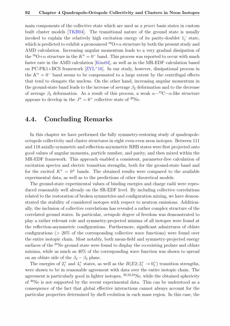
92 Chapter 4 Quadrupole-Octupole Collectivity and Clusters in Neon Isotopes
main components of the collective state which are used as a priori basis states in custom
built cluster models [TKH04]. The transitional nature of the ground state is usually
invoked to explain the relatively high excitation energy of its parity-doublet 1−1 state,
which is predicted to exhibit a pronounced 16O+α structure by both the present study and
AMD calculation. Increasing angular momentum leads to a very gradual dissipation of
the 16O+α structure in the Kπ = 0− band. This process was reported to occur with much
faster rate in the AMD calculation [Kim04], as well as in the MR-EDF calculation based
on PC-PK1+BCS framework [ZYL+16]. In our study, however, dissipational process in
the Kπ = 0− band seems to be compensated to a large extent by the centrifugal effects
that tend to elongate the nucleus. On the other hand, increasing angular momentum in
the ground-state band leads to the increase of average β2 deformation and to the decrease
of average β3 deformation. As a result of this process, a weak α−12C−α-like structure
appears to develop in the Jπ = 6+ collective state of 20Ne.
4.4. Concluding Remarks
In this chapter we have performed the fully symmetry-restoring study of quadrupole-
octupole collectivity and cluster structures in eight even-even neon isotopes. Between 111
and 118 axially-symmetric and reflection-asymmetric RHB states were first projected onto
good values of angular momenta, particle number, and parity, and then mixed within the
MR-EDF framework. This approach enabled a consistent, parameter-free calculation of
excitation spectra and electric transition strengths, both for the ground-state band and
for the excited Kπ = 0± bands. The obtained results were compared to the available
experimental data, as well as to the predictions of other theoretical models.
The ground-state experimental values of binding energies and charge radii were repro-
duced reasonably well already on the SR-EDF level. By including collective correlations
related to the restoration of broken symmetries and configuration mixing, we have demon-
strated the stability of considered isotopes with respect to neutron emissions. Addition-
ally, the inclusion of collective correlations has revealed a rather complex structure of the
correlated ground states. In particular, octupole degree of freedom was demonstrated to
play a rather relevant role and symmetry-projected minima of all isotopes were found at
the reflection-asymmetric conifgurations. Furthermore, significant admixtures of oblate
configurations (> 20% of the corresponding collective wave functions) were found over
the entire isotopic chain. Most notably, both mean-field and symmetry-projected energy
surfaces of the 24Ne ground state were found to display the co-existing prolate and oblate
minima, while as much as 40% of the corresponding wave function was shown to spread
on an oblate side of the β2 − β3 plane.
The energies of 2+1 and 4+
1 states, as well as the B(E2; 2+1 → 0+
1 ) transition strengths,
were shown to be in reasonable agreement with data over the entire isotopic chain. The
agreement is particularly good in lighter isotopes, 20,22,24Ne, while the obtained sphericity
of 30Ne is not supported by the recent experimental data. This can be understood as a
consequence of the fact that global effective interactions cannot always account for the
particular properties determined by shell evolution in each mass region. In this case, the

4.4 Concluding Remarks 93
erosion of the N = 20 shell closure in very neutron-rich nuclei is simply not reproduced by
the DD-PC1 functional. Nevertheless, it was shown that the further addition of neutrons
leads to development of a strong prolate deformation in the most neutron-abundant neon
isotope, 34Ne. This nucleus exhibits a pronouncedly compressed ground-state band as
compared to other isotopes, with the lowest excitation energies of 2+1 and 4+
1 states over
the entire isotopic chain. Additionally, signatures of the ground-state shape-coexistence
were demonstrated to survive in the excited states of 24Ne isotope. In particular, its 6+1
still contains almost 40% contribution from the oblate configurations, while 0+2 and 2+
2
states in this isotope are found at much lower energies than the corresponding states in22Ne isotope.
Finally, we have paid special attention to the case of the self-conjugate 20Ne isotope.
The obtained spectroscopic properties were thoroughly compared to the experimental
data, as well as to the predictions of two other theoretical models. In particular, our
calculation was shown to exhibit a level of accuracy that this comparable to the one ob-
tained using more specific models, such as the antisymmetrized molecular dynamics. The
ground state of 20Ne was demonstrated to have predominantly 16O+α structure, while
about 25% of its collective wave function corresponds to the oblate-deformed 2α+12C-
like structure. The increase of angular momentum leads to the predominance of prolate
shapes and a gradual dissolution of the 16O+α structure. In the negative-parity band
this dissolution occurs at much slower rate than reported in previous studies, while in
the positive-parity band it leads towards development of the α−12C−α-like structure in
Jπ = 6+ state.


Chapter 5
Cluster Structures in 12C Isotope
Nothing in life is to be feared, it is only to be understood.
Now is the time to understand more, so that we may fear less.
Marie Curie, as quoted in ”Our Precarious Habitat” by M. A. Benarde
Formation of clusters, transitional states between quantum liquid and solid phases of
finite systems, is a common feature in light atomic nuclei [Bec10, Bec12, Bec14, HIK12,
FHKE+18]. Particularly favorable conditions for the appearance of cluster structures are
found in light self-conjugate nuclei, where various exotic configurations are thought to
be formed. Probably one of the most striking examples is the self-conjugate 12C isotope,
where axial oblate, triangular, linear 3α, and bent arm configurations are all predicted to
exist in the low-lying structure [KE07, NF04, CFN+07, THSR01, Fun15, FSF+13]. The
ground state of 12C lies about 7.3 MeV below the α-decay threshold. Therefore, cluster
structures are expected to be significantly suppressed in the lowest 0+ state, as it exhibits
a more compact intrinsic density distribution. The Kπ = 0+1 rotational band built upon
the ground state consists of the 2+1 state at 4.4 MeV and the 4+
1 state at 14.1 MeV.
Very recently, new reorientation-effect measurements in the 2+1 state have confirmed its
pronounced oblate deformation through the relatively large and positive value of the cor-
responding spectroscopic quadrupole moment [R+18]. Furthermore, the 0+2 state at 7.65
MeV, the famous Hoyle state, is arguably one of the most studied collective nuclear states
overall [FF14, THSR17], largely due to the fact that it plays a major role in the stellar
nucleosynthesis of 12C through the so-called triple-α process. In particular, the presence
of the Hoyle state resonantly boosts the capture process of an α-particle on 8Be by more
than 10 million times, thereby making a decisive impact on the abundance of 12C isotope
in the universe and, consequently, the appearance of organic life on Earth. Remarkable
results on the structure of the Hoyle state have recently been simultaneously reported
by two independent groups of researchers [D+17, SKW+17], strongly indicating that the
Hoyle state predominantly decays through an intermediate emission of an α-particle. In
95

96 Chapter 5 Cluster Structures in 12C Isotope
parallel with experimental advances, various theoretical approaches have been employed
to study rich variety of shapes in 12C, including the antisymmetrized molecular dynam-
ics model [KE07], the fermionic molecular dynamics model [NF04, CFN+07], the THSR
wave function model [THSR01, Fun15], the configuration mixing Skyrme calculations
with Gaussian wave packets [FSF+13], and the cranked RMF theory [RZZ+18]. Both
AMD and FMD calculations predict for the Hoyle state to be dominated by a weakly-
interacting assembly of 8Be+α configurations [KE07, CFN+07], while the THSR model
describes Hoyle state in terms of an actual condensate of α-particles [THSR01]. Fur-
thermore, 3α linear chain structures were predicted to exist in higher 0+ states of 12C
[KE07, CFN+07], even though the stability of these configurations against bending still
remains an open question [RZZ+18]. A detailed review on recent experimental and the-
oretical advances in studies of cluster structures in light nuclei and, particularly, in the12C isotope can be found in Ref. [FHKE+18]. Additionally, structure of the Hoyle state
has been a subject of multiple dedicated review papers (see, for example, Refs. [FF14]
and [THSR17]).
In this chapter, we will employ the previously described MR-EDF model in a study of
collective spectroscopy and cluster structures in 12C isotope [MEK+18b]. A wide range
of quadrupole- and octupole-deformed axially-symmetric RHB states are projected onto
good values of angular momenta, particle numbers, and parity, and further mixed in or-
der to build the symmetry-conserving positive-parity collective states. In Section 5.1.1
we analyze the potential energy surface of 12C, both on the mean-field and symmetry-
conserving level. Furthermore, in Sec 5.1.2 we present the spectroscopic results for 12C
in comparison to the available data and to predictions of other theoretical models. The
structure of the collective states in the intrinsic frame is discussed in Sec. 5.1.3, while
in Sec. 5.1.4 we present the results for both the elastic and inelastic form factors for
electron-12C scattering.

5.1 Structure of the 12C Isotope 97
−1.2 −0.6 0.0 0.6 1.2 1.8 2.4 3.0
0.5
1.0
1.5
2.0
2.5
3.0
3.5
β3
0.0
12CRHB
−1.2 −0.6 0.0 0.6 1.2 1.8 2.4 3.0
0.5
1.0
1.5
2.0
2.5
3.0
3.5
12CJπ =0+
−1.2 −0.6 0.0 0.6 1.2 1.8 2.4 3.0β2
0.5
1.0
1.5
2.0
2.5
3.0
3.5
β3
0.0
12CJπ =2+
−1.2 −0.6 0.0 0.6 1.2 1.8 2.4 3.0β2
0.5
1.0
1.5
2.0
2.5
3.0
3.5
12CJπ =4+
0
5
10
15
20
25
EB[MeV
]
Figure 5.1: Potential energy surfaces of 12C isotope in the β2 - β3 plane. In addition to theself-consistent RHB binding energies (the upper left panel), we display the angular momentum-,particle number-, and parity-projected energy surfaces for spin-parities Jπ = 0+, 2+, 4+. Foreach surface, energies are normalized with respect to the energy of the corresponding absoluteminimum. Dashed contours are separated by 2.5 MeV.
5.1. Structure of the 12C Isotope
5.1.1 Potential Energy Maps
We begin our analysis with the self-consistent RHB calculation, performed by expand-
ing nuclear spinors in the configuration space of axially-symmetric harmonic oscillator
with Nsh = 10 major oscillator shells for the large and Nsh = 11 for the small component
of spinor. This calculation covers a wide range of deformations in both the quadrupole
and octupole direction, β2 ∈ [−1.2, 3.6] and β3 ∈ [−3.5, 3.5], with steps in the oblate,
prolate, and octupole direction being ∆β2 = 0.4, ∆β2 = 0.6, and ∆β3 = 0.7, respectively.
The calculated potential energy surfaces are shown in the upper left panel of Figure 5.1.
Although the absolute minimum of the RHB energy surface is found for the spherical
(β2 = 0, β3 = 0) configuration, we note that the surface is rather soft for the following
range of deformations: β2 ≈ [−0.6, 0.6] and |β3| ≈ [0.0, 0.5]. In order to demonstrate
the influence of symmetry restoration on the topology of the RHB surface, other panels

98 Chapter 5 Cluster Structures in 12C Isotope
-1.2 -0.8 -0.4 0.0 0.4 0.8 1.2 1.6 2.0 2.4 2.8 3.2 3.6β2
-94
-90
-86
-82
-78
-74
-70
-66EB
[MeV
]
RHBN&Z, J=0N&Z, J=2N&Z, J=4
Figure 5.2: Potential energy curves of 12C isotope as functions of axial quadrupole deformationβ2 for parity-conserving (β3 = 0) configurations. In addition to the self-consistent RHB bindingenergies (squares), we display angular momentum- and particle number-projected curves forspin-parities Jπ = 0+, 2+, 4+ .
of Fig. 5.1 show the corresponding angular momentum-, particle number-, and parity-
projected energy surfaces for spin-parity values Jπ = 0+, 2+, 4+. Already a glance at the
Jπ = 0+ energy surface unveils a dramatic impact of performing the symmetry restora-
tion. In particular, the Jπ = 0+ energy surface appears significantly softer for a wide
range of deformations in comparison to the RHB energy surface. For higher values of
angular momentum, the minimum at the oblate side becomes much more pronounced,
while intermediate prolate deformations become increasingly less energetically favored.
This trend is even more apparent in Figure 5.2, where we make a cut along the parity-
conserving (β3 = 0) line of Fig. 5.1 and show the potential energy curves as functions
of axial quadrupole deformation β2. As noted before, the RHB potential energy curve is
very flat around the spherical minimum, both in the prolate and oblate direction. The
only indication of possible clusterized structures is found at very large prolate deforma-
tions, where a shoulder in binding energy curve is formed. On the other hand, energy
curve of the symmetry-restored Jπ = 0+ state exhibits two nearly-degenerate minima:
the absolute oblate minimum at β2 ≈ −0.5 and the prolate minimum at β2 ≈ 0.8. We
note that the binding energy of the symmetry-restored oblate minimum from Fig. 5.2
is very close to the experimental binding energy EexpB = −92.16 MeV. This is consistent
with the fact that the collective 0+1 state is expected to correspond to the band-head of
an oblate-deformed rotational band. Furthermore, shoulder at large quadrupole defor-
mations is preserved by projections for the Jπ = 0+ curve and it is additionally lowered
by about 5 MeV. The Jπ = 2+ projected curve preserves both the oblate minimum and
the shoulder at large quadrupole deformations, while the former Jπ = 0+ local minimum
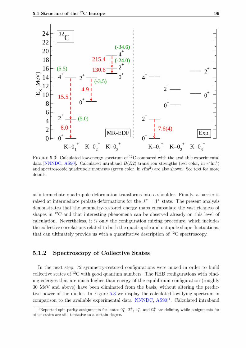
5.1 Structure of the 12C Isotope 99
02468
1012141618202224
EX
[M
eV]
K=02
+K=0
3
+0
+
4+
2+
0+
2+ 0
+
2+
4+
0+
12C
2+
4+
0+
2+
0+
K=01
+
2+
K=01
+K=0
3
+
8.0
15.54.9
130.6
215.4
(5.0)
(5.5)
(-3.5)
(-24.0)
(-34.6)
7.6(4)
K=02
+
MR-EDF Exp.
Figure 5.3: Calculated low-energy spectrum of 12C compared with the available experimentaldata [NNNDC, AS90]. Calculated intraband B(E2) transition strengths (red color, in e2fm4)and spectroscopic quadrupole moments (green color, in efm2) are also shown. See text for moredetails.
at intermediate quadrupole deformation transforms into a shoulder. Finally, a barrier is
raised at intermediate prolate deformations for the Jπ = 4+ state. The present analysis
demonstrates that the symmetry-restored energy maps encapsulate the vast richness of
shapes in 12C and that interesting phenomena can be observed already on this level of
calculation. Nevertheless, it is only the configuration mixing procedure, which includes
the collective correlations related to both the quadrupole and octupole shape fluctuations,
that can ultimately provide us with a quantitative description of 12C spectroscopy.
5.1.2 Spectroscopy of Collective States
In the next step, 72 symmetry-restored configurations were mixed in order to build
collective states of 12C with good quantum numbers. The RHB configurations with bind-
ing energies that are much higher than energy of the equilibrium configuration (roughly
30 MeV and above) have been eliminated from the basis, without altering the predic-
tive power of the model. In Figure 5.3 we display the calculated low-lying spectrum in
comparison to the available experimental data [NNNDC, AS90]1. Calculated intraband
1Reported spin-parity assignments for states 0+1 , 2+1 , 4+1 , and 0+2 are definite, while assignments forother states are still tentative to a certain degree.

100 Chapter 5 Cluster Structures in 12C Isotope
−1.0 −0.5 0.0 0.5 1.0 1.5 2.0 2.5 3.0 3.50.0
0.5
1.0
1.5
2.0
β3
12CJ πα =0+
1
0.025 0.050 0.075|g(β2 ,β3 )|2
0.00 0.10
−1.0 −0.5 0.0 0.5 1.0 1.5 2.0 2.5 3.0 3.5
0.0
0.5
1.0
1.5
2.0
12CJ πα =0+
2
0.05 0.10 0.15|g(β2 ,β3 )|2
0.00 0.20
−1.0 −0.5 0.0 0.5 1.0 1.5 2.0 2.5 3.0 3.5
0.0
0.5
1.0
1.5
2.0
12CJ πα =0+
3
0.02 0.04 0.06|g(β2 ,β3 )|2
0.00 0.08
−1.0−0.5 0.0 0.5 1.0 1.5 2.0 2.5 3.0 3.5β2
0.0
0.5
1.0
1.5
2.0
β3
12CJ πα =2+
1
0.05 0.10 0.15|g(β2 ,β3 )|2
0.00 0.20
−1.0−0.5 0.0 0.5 1.0 1.5 2.0 2.5 3.0 3.5β2
0.5
1.0
1.5
2.0
12CJ πα =2+
2
0.07 0.14 0.21|g(β2 ,β3 )|2
0.00 0.28
−1.0−0.5 0.0 0.5 1.0 1.5 2.0 2.5 3.0 3.5β2
0.0
0.5
1.0
1.5
2.0
12CJ πα =2+
3
0.02 0.04 0.06|g(β2 ,β3 )|2
0.00 0.08
Figure 5.4: Amplitudes of collective wave functions squared |g(β2, β3)|2 of the low-energylevels in 12C. Dashed contours in the β2 − β3 plane successively denote a 10% decrease startingfrom the largest value of the amplitude.
B(E2) transition strengths and spectroscopic quadrupole moments of collective states are
also shown. The calculated excitation energies of 2+1 (4.3 MeV) and 4+
1 (13.9 MeV) states
are only slightly lower than the corresponding experimental values. In addition, their
ratio E(4+1 )/E(2+
1 ) = 3.23 is in very good agreement with the experimental value of 3.17,
strongly indicating a rotational character of the ground-state band. Furthermore, calcu-
lated E2 transition strength from the 2+1 state to the ground state, B(E2; 2+
1 → 0+1 ) = 8.0
e2fm4, is in very good agreement with the experimental value. We also note that the cal-
culated spectroscopic quadrupole moment of 2+1 state, Qspec(2
+1 ) = 5.0 efm2, is within the
error bar margin of the very recently obtained experimental value, Qexpspec(2
+1 ) = 7.1± 2.5
efm2 [R+18]. It is therefore interesting to mention that, in this specific instance, the
global EDF model provides the level of agreement with the experimental data that is
comparable to the one provided by the state-of-the-art ab initio model reported therein
[R+18]. Finally, calculated B(E2; 4+1 → 2+
1 ) = 15.5 e2fm4 value is in excellent agree-
ment with the AMD prediction B(E2; 4+1 → 2+
1 ) = 16 e2fm4 [KE07]. Measurements of
this quantity are yet to be performed and they would definitely confirm the rotational
character of the ground-state band. On the other hand, the second 4+ state within our
calculation is characterized by a pronouncedly enhanced value of quadrupole deformation
parameter, a feature that is shared by the 0+3 and 2+
3 collective states. In addition, it
exhibits a very strong E2 transition strength to the 2+3 state. Therefore, it is assigned
to the Kπ = 0+3 band and denoted as 4+
3 further on. Both very large E2 intraband
transitions and the value of ratio (E(4+3 )− E(0+
3 ))/(E(2+3 )− E(0+
3 )) = 3.45 strongly in-
dicate the rotational character of this band. Additionally, huge spectroscopic quadrupole
moments of 4+3 and 2+
3 states support the interpretation of this band as the 3α linear

5.1 Structure of the 12C Isotope 101
chain. Calculated value of B(E2; 2+3 → 0+
3 ) = 130.6 e2fm4 is somewhat larger than the
one reported in Ref. [KE07], but still of the same order of magnitude. Furthermore,
the 0+2 (Hoyle) state in our study is found at excitation energy that is less than 1 MeV
above the experimental value. However, calculated E2 transition strength from the corre-
sponding 2+2 state is about an order of magnitude smaller than the one obtained in AMD
[KE07] and THSR [Fun15] calculations. Even though there are currently no available
experimental values that would settle this disagreement, it is likely that our calculation
actually underestimates the true value. The reason for this is at least two-fold. Firstly,
AMD and THSR models consistently predict for the dominant contribution to the Hoyle
state intrinsic density to stem from triaxial configurations. As noted before, these con-
figurations are not included in the present study and an extended study that includes
triaxial shapes would be required in order to draw some fairer comparisons. In addition,
the asymptotic behavior of three weakly-interacting α particles is notoriously complicated
to describe within the harmonic oscillator basis [NGV+07, Nef12]. Therefore, it remains
an open question whether the self-consistent models based on harmonic oscillator expan-
sions, even once the triaxial shapes have been included, will be able to encompass all
the details of the Hoyle state density profile. Nevertheless, we note that the calculated
transition strength from the 2+1 state to the Hoyle state, B(E2; 2+
1 → 0+2 ) = 1.7 e2fm4
compares quite favorably to the experimental value 2.6± 0.4 e2fm4 and to the AMD (5.1
e2fm4) predictions [KE07]. In addition, even the transition strength from the 2+2 state
to the ground state, B(E2; 2+2 → 0+
1 ) = 1.3 e2fm4, is of at least comparable quality as
THSR prediction (2.0 − 2.5 e2fm4) [Fun15] when compared to the experimental value
(0.73± 0.13 e2fm4).
5.1.3 Structure of Collective States in the Intrinsic Frame
In Figure 5.4 we show amplitudes of collective wave functions squared |g(β2, β3)|2 of
the low-energy levels in 12C. Even though they are not observables, these wave functions
provide us with a measure of quadrupole and octupole shape fluctuations in collective
states. Moreover, they can be used to calculate averaged values of deformation parame-
ters (β2, β3) for each collective state. These values are subsequently used to represent the
density distributions of the collective states in the intrinsic frame of reference [see Sec.
4.3.2]. Intrinsic density distributions for the three lowest 0+ and 2+ states in 12C isotope
are displayed in Figure 5.5. For each state, the corresponding prolate and/or oblate de-
formation parameters (β2, β3), as well as the respective contribution of prolate or oblate
configurations to the total collective wave function, are given. Only 0+1 and 0+
2 states ex-
hibit significant contributions from both the prolate and oblate configurations, while other
states display predominance of either prolate or oblate shapes. In particular, situation in
the 0+1 state is rather similar to the one encountered in the symmetry-restored Jπ = 0+
potential energy curve of Fig. 5.2, where prolate-deformed local minimum coexists with
the oblate-deformed absolute minimum. In fact, maximum of the 0+1 collective wave func-
tion is also found at the oblate-deformed (β2, β3) = (−0.4, 0.0) configuration. However,
|g(β2, β3)|2 has non-negligible contributions from configurations in a rather wide range of

102 Chapter 5 Cluster Structures in 12C Isotope
-5-4-3-2-10
12345
z [fm
]2+
1
(-0.45,0.55) 90%
2+2
(0.64,0.48) 86%
0+3
(2.28,0.71) 92%
2+3
(2.31,0.68) 99%
-4-3-2-1 0 1 2 3 4x [fm]
-5-4-3-2-10
12345
z [fm
]
0+1
(-0.34,0.51) 65%
-4-3-2-1 0 1 2 3 4x [fm]
0+1
(0.83,0.67) 35%
-4-3-2-1 0 1 2 3 4x [fm]
0+2
(0.23,0.59) 59%
-4-3-2-1 0 1 2 3 4x [fm]
0+2
(-0.70,0.55) 41%
0.000.020.040.060.080.100.120.140.160.18
ρin
t [fm
−3]
Figure 5.5: Characteristic intrinsic nucleon densities of the first three 0+ and 2+ collectivestates in 12C. The corresponding average deformation parameters (β2, β3), as well as the respec-tive contributions of prolate and/or oblate configurations, are given. The lower panel displaysstates that exhibit significant both prolate and oblate contributions, while the upper panel dis-plays states that are predominantely characterized by either prolate or oblate configuration. Seetext for more details.
deformations, roughly β2 ∈ [−1.2, 1.2] and |β3| ∈ [0.0, 1.4]. Averaging over all these con-
figurations incorporates significant contributions from prolate configurations that balance
the influence of oblate maximum and would ultimately yield the nearly-spherical density
distribution. This clearly does not reflect the actual physical picture of the 12C ground
state. Therefore, we follow the prescription of Section 4.3.2 and calculate the correlated
(β2, β3) values by averaging over the prolate-deformed and oblate-deformed configura-
tions separately, using the collective wave functions as the corresponding weights [see
Eqs. (2.40) and (2.41)]. The two plots in the lower left panel of Fig. 5.5 display the
obtained densities, as well as the respective contributions of prolate and oblate configura-
tions to the total collective wave function2. These densities reflect the complex structure
of the 12C ground state, where the maximum of |g(β2, β3)|2 is found at an oblate con-
figuration while tail of the wave function spreads deeply into the prolate side of the
β2 − β3 plane. On the other hand, collective wave function of the 2+1 state is predomi-
nantly spread over the (β2 < 0, β3) configurations and the obtained density distribution
is oblate-deformed. This can be understood as a consequence of the sway towards oblate
shapes in the Jπ = 2+ energy maps of Figs. 5.1 and 5.2, and it is in agreement with the
2We note that some authors compute the characteristic density of a collective state by using config-uration that corresponds to the collective wave function maximum [see, for example, Ref. [ZYL+16]].With this choice, intrinsic density of 0+1 state in the present would exhibit the oblate-deformed reflection-symmetric shape. Nevertheless, for the sake of consistency, we follow the prescription of Chapter 4 andadopt the averaged (β2, β3) values as representative deformation parameters.

5.1 Structure of the 12C Isotope 103
relatively large and positive spectroscopic quadrupole moment of the 2+1 state. Moreover,
intrinsic nucleon density of the 4+1 state is characterized by the (β2, β3) = (−0.50, 0.58)
configuration, clearly pointing towards oblate nature of the ground-state band. Further-
more, collective wave function of the 0+2 state exhibits two maxima: one at the small
prolate deformations and the other one at larger oblate deformations. The corresponding
density distributions are obtained equivalently to the 0+1 case and they are displayed in
the lower right panel of Fig. 5.5. Of course, in order to obtain the expected triangular
distribution of the Hoyle state one needs to break the axial symmetry, which is out of the
scope of the present work. Finally, the Kπ = 0+3 band originates from the shoulder at
large β2 values in Figs. 5.1 and 5.2. In the intrinsic frame of reference, a large quadrupole
deformation translates into a pronounced linear structure of 0+3 and 2+
3 collective states,
as seen in the upper right panel of Fig. 5.5. The homogeneous alignment of 3α particles
would be described by a reflection-symmetric configuration in the intrinsic frame, that
is, the corresponding octupole deformation parameter would be negligible. Even though
the maxima of 0+3 and 2+
3 wave functions are indeed found at β3 = 0 configurations
[see Fig. 5.4], fluctuations in octupole direction are rather pronounced in both states.
Consequently, the reflection-asymmetric 8Be+α-like structure is formed in the intrinsic
frame. Formation of linear chain structures in 12C isotope has been previously predicted
by some theoretical calculations [KE07, NF04], even though they are yet to be confirmed
experimentally. Another interesting feature of 3α linear chains is their alleged suscepti-
bility to bending, which would eventually lead to the formation of bent arm structures
[KE07, NF04, RZZ+18]. However, besides breaking reflection symmetry, such structures
additionally break the axial symmetry and they are therefore not included in the present
study.
5.1.4 Electron Scattering Form Factors
Additional insight into the structure of collective states is provided by the form factors
of the electron-nucleus scattering. Formalism for calculating these quantities within the
MR-EDF framework was introduced only recently [YBH15] and details related to our
implementation are available in Appendix B.2. In this subsection, we will calculate form
factors for electron scattering from 12C for 0+1 → 0+
1 (elastic) and 0+1 → 0+
2 (inelastic)
transitions. The basic ingredients of the calculation are collective wave functions, dis-
played in Fig. 5.4. As noted before, both for the 0+1 and for the 0+
2 state these wave
functions are concentrated in the −1.2 ≤ β2 ≤ 1.2 and 0 ≤ |β3| ≤ 1.4 part of the β2 - β3
plane. Therefore, in order to reduce the computational cost and without neglecting any
physical content, only configurations within that range are included in the subsequent
calculation of form factor. In the upper panel of Figure 5.6 we show the calculated form
factors |F0(q)|2 for elastic 0+1 → 0+
1 scattering in comparison with the available experi-
mental data. In addition, the inset shows the corresponding charge density, calculated
as ρch(r) = ρ0101,0(r)/
√4π, where ρ01
01,0(r) is the diagonal element of the reduced transi-
tion density that enters the calculation of form factor [see Eq. (2.44)]. Our results for
the form factor are compared with predictions of two other theoretical models, namely,

104 Chapter 5 Cluster Structures in 12C Isotope
0 2 4 6 8 10 12q
2 [fm
-2]
1e-09
1e-08
1e-07
1e-06
1e-05
1e-4
0.001
0.01
0.1
1
|F(q
)|2MR-EDF AMDTHSRExp.
0 2 4 6 8r [fm]
0
0.02
0.04
0.06
0.08
ρch
[fm
-3]
01
+→ 0
1
+
(a)
0 2 4 6 8 10 12q
2 [fm
-2]
1e-09
1e-08
1e-07
1e-06
1e-05
1e-4
0.001
0.01
|F(q
)|2
MR-EDF AMDTHSRExp.
0 2 4 6 8r [fm]
-0.050
0.050.1
0.15
ρtr r
4 [fm
]
01
+→ 0
2
+
(b)
Figure 5.6: Form factors of electron scattering from 12C for 0+1 → 0+
1 (upper panel) and0+
1 → 0+2 (lower panel) transitions. Results obtained within our model are compared to the
available experimental data for the elastic [SM70, NTH71, SS68] and inelastic [CFN+10] formfactors, as well as to predictions of AMD [KE07] and THSR [FTH+06] models. In addition,insets show the corresponding charge density (upper panel) and the transition charge density(lower panel). See text for more details.

5.1 Structure of the 12C Isotope 105
the antisymmetrized molecular dynamics model and the Tohsaki-Horiuchi-Schuck-Ropke
wave function model. The AMD calculations [KE07] treat single nucleons as relevant de-
grees of freedom, describing them in terms of Gaussian wave packets. On the other hand,
THSR framework is explicitly built as the α-cluster model, that is, the relevant degrees
of freedom are α-particles in Bose-condensed state [FTH+06]. In the low momentum-
transfer region (q2 < 2 fm2) all models yield similar predictions for the elastic form
factor. However, for larger values of the momentum transfer the difference between the
three curves becomes visible. In particular, the first zero of |F0(q)|2 is found at roughly
q2 ≈ 3 fm2 both in our and in the THSR calculation, while the AMD calculation predicts
this zero at somewhat smaller value of the momentum transfer. Details of the elastic
form factors can be traced back to the properties of the corresponding charge distribu-
tion [FV82, FVR86]. The shift of the position of the first zero towards smaller values of
q2, in particular, can be attributed to the larger spatial extension of the charge density.
Furthermore, the amplitude of the first |F0(q)|2 maximum is related to the surface thick-
ness of the charge distribution. Larger values of surface thickness yield smaller values of
the first maximum, and vice versa. We note that the experimental position and ampli-
tude of the first |F0(q)|2 maximum are reproduced rather nicely by all models. At very
large values of q2 the THSR model provides the best agreement with the experiment,
while our calculation underestimates experimental values. Similar behavior has been ob-
served in Ref. [YBH15] for the case of 24Mg and in Ref. [FSF+13] for the case of 12C,
where it was argued that the spreading of collective wave function over many deforma-
tions generates too large smoothing of the one-body density and thus decreases weights
of the large-momentum components of the transition density. Finally, due to its short
lifetime, elastic scattering experiments for the Hoyle state have not yet been performed.
Therefore, its structure is usually probed via the inelastic scattering experiments from
the ground state. In the lower panel of Fig. 5.6 we display the calculated form factors for
0+1 → 0+
2 scattering in comparison with the available experimental data and predictions of
the AMD and THSR models. Our calculations reproduce nicely the position of the first
maximum, even though the corresponding amplitude is underestimated in comparison
to both the experiment and two theoretical models. On the other hand, position of the
first zero is reproduced well by all three models. In addition, our model displays good
agreement with the experiment up to rather large q2 values. The inset in the lower panel
of Fig. 5.6 displays the corresponding transition charge density, ρtr(r) = ρ0201,0(r)/
√4π,
where ρ0201,0(r) is the non-diagonal element of the reduced transition density that enters
the calculation of form factor [see Eq. (2.44)]. Our prediction for ρtr(r)r4 can be directly
compared to the experimental transition charge density corresponding to the form factor
of Fig. 5.6 [CFN+10], as well as to the predictions of the FMD model and the α-cluster
model that are plotted in Fig. 3 of Ref. [CFN+10]. While the position of the minimum of
ρtr(r)r4 is very similar for all four curves considered, our calculation predicts somewhat
smaller amplitude in comparison to both the experiment and other models. Furthermore,
FMD and α-cluster model overestimate the experimental maximum value of the ρtr(r)r4
curve, located at r ≈ 4 fm. Our calculation, on the other hand, notably underestimates
it. This difference is then naturally reflected in the underestimated value of form factor
in comparison to the experiment, particularly at low values of momentum transfer. The
inclusion of triaxial degree of freedom, that undeniably plays an important role in the 0+2

106 Chapter 5 Cluster Structures in 12C Isotope
state, would likely modify the calculated transition charge density and, consequently, the
corresponding form factor. Whether such an upgrade to the model will actually bring
the expected shift towards experimental values3 remains to be examined in the future.
5.2. Concluding Remarks
In this chapter, we have performed the fully symmetry-conserving study of the low-
lying spectroscopy and cluster structures in 12C isotope. Axially-symmetric and reflection-
asymmetric RHB states were first projected onto good values of angular momenta, particle
number, and parity, and then mixed within the MR-EDF framework. Starting from an
effective interaction that was fitted to data on heavy nuclei and a formalism that does not
a priori assume any clusterized structures, the employed framework enabled a consistent,
parameter-free calculation of collective excitation spectra and the corresponding electric
transition strengths in the very light 12C isotope.
In particular, we have focused our attention on the structure of the three lowest Kπ =
0+ bands. Overall, empirical properties of the ground-state band have been accurately
reproduced. Collective 2+1 and 4+
1 states are found at energies that are only marginally
lower than the experimental values, and the corresponding ratio E(4+1 )/E(2+
1 ) strongly
indicates the rotational character of the yrast band. Moreover, calculated E2 transition
strength from the 2+1 state to the ground state is within the experimental error bar
margin, while positive spectroscopic quadrupole moments confirm oblate deformation of
the Kπ = 0+1 band. The present model does not include triaxial shapes and it therefore
does not reproduce the B(E2; 2+2 → 0+
2 ) strength within the Hoyle band as calculated
with the AMD and the THSR theoretical models. Nevertheless, the obtained 0+2 state is
located less than 1 MeV above its measured position, and the calculated B(E2; 2+1 → 0+
2 )
strength is in rather good agreement with the experiment. Furthermore, the excited band
built upon the 0+3 state was demonstrated to have a strong rotational character with rather
large spectroscopic quadrupole moments and intraband E2 transition strenghts. In the
intrinsic frame, this band exhibits the pronounced linear chain structure that corresponds
to the 8Be+α configuration. Finally, both elastic and inelastic form factors show good
agreement with the experimental data for a rather wide range of momentum transfers.
In this particular aspect, the present global model exhibits a predictive power which can
compete with that of the most successful models for cluster studies.
3Remember the morals of footnote 4 on p. 84.


Conclusion and Outlook
Three passions, simple but overwhelmingly strong, have governed my life: the longing for
love, the search for knowledge, and unbearable pity for the suffering of mankind. These
passions, like great winds, have blown me hither and thither, in a wayward course, over a
great ocean of anguish, reaching to the very verge of despair. (...) This has been my life.
I have found it worth living, and would gladly live it again if the chance were offered me.
Bertrand Russell, Prologue to Autobiography
The framework of energy density functionals currently provides the most complete and
accurate description of ground-state and excited-state properties of atomic nuclei over
the entire nuclide chart. EDF-based models, especially when extended to include the
restoration of broken symmetries and subsequent configuration mixing, represent state-
of-the-art tool for studies of various structure phenomena, from light nuclear systems
to superheavy nuclei and from the valley of β-stability to the particle drip-lines. Some
of the advantages of using manifestly covariant functionals involve the natural inclusion
of the spin-orbit potential, the unique parameterization of nucleon currents, as well as
the explanation of empirical pseudospin symmetry in terms of relativistic mean-fields.
Recently, it was also demonstrated that relativistic EDFs, when compared to their non-
relativistic counterparts, predict significantly more localized density distributions in light
nuclei. This property of covariant framework was linked to the larger depth of the under-
lying single-nucleon potential, which corresponds to a sum of the large attractive scalar
and repulsive vector Lorentz fields. In practical terms, this feature makes relativistic EDF
models a particularly convenient framework for studies of formation of clusters, that can
be considered as a transitional phenomenon between quantum liquid and solid phases in
atomic nuclei.
In this thesis, we have developed the fully symmetry-conserving collective model for
nuclear structure studies based on the relativistic EDF framework. Starting point of our
calculation was the RHB model, which provides a unified description of particle-hole and
particle-particle correlations on a mean-field level. In the ph channel we have used the
point-coupling DD-PC1 functional, while a pairing force separable in momentum space
was employed in the pp channel. Both axial and time-reversal symmetry of the intrinsic
states were imposed, while they were allowed to break the rotational, particle number,
and parity symmetry. This kind of analysis enabled an access to nuclear configurations
109

110
in the entire plane spanned by the axially-symmetric quadrupole and octupole deforma-
tions, providing a basic description of nuclear ground-states in terms of the symmetry-
breaking wave functions. In the next step, the restoration of angular momentum, particle
number, and parity of intrinsic states were all simultaneously performed. The symmetry-
restored configurations were further mixed within the MR-EDF framework in order to
build collective nuclear states with good quantum numbers. Solving the corresponding
HWG equation yielded the excitation spectra and collective wave functions that could
then be used to calculate various observables, such as spectroscopic quadrupole moments
and electromagnetic multipole transition strengths. Finally, the recently-developed BMF
techniques for studies of correlated densities and electron scattering form factors were
implemented to the model. Ultimately, we have developed the state-of-the-art collective
model for nuclear structure studies that can, together with the eventual extensions, be
applied in analyses of various phenomena over the entire nuclide chart. In this work, the
model was employed in a study of clustering phenomena in neon and carbon isotopes.
Starting from an effective interaction that was fitted to data on medium-heavy and heavy
nuclei and a formalism that does not a priori assume any clusterized structures, the em-
ployed framework enabled a consistent, parameter-free calculation of collective excitation
spectra and the corresponding electric transition strengths in light and very light nuclear
systems.
As a first application of the model, we have carried out a comprehensive study of
quadrupole-octupole collectivity and cluster structures in neon isotopes. The ground-
state experimental values of binding energies and charge radii were reproduced reasonably
well already on the SR-EDF level. On the MR-EDF level, correlated ground states were
demonstrated to exhibit a rather complex structure, with significant contributions from
both the prolate- and oblate-deformed configurations. The corresponding two-neutron
separation energies showed good agreement with the experimental data, and 34Ne is
confirmed to be the last stable even-even isotope of neon. Furthermore, good agree-
ment with the experimental low-lying excitation energies and transition strengths was
obtained over the entire isotopic chain. Signatures of the shape-coexistence were detected
in 24Ne isotope, while the drip-line 34Ne nucleus was found to exhibit a prolate-deformed
structure with significantly compressed collective spectrum. Calculated spectrum for the
self-conjugate 20Ne isotope was shown to exhibit a level of accuracy that is comparable
to the one obtained using some more specific models, such as the AMD theory. It was
demonstrated that the obtained lowest positive- and negative-parity doublet bands are
dominated by the 16O+α structure in the intrinsic frame. The ground state of 20Ne con-
tains significant contribution from oblate-deformed configurations, while the increase of
angular momentum leads towards predominance of prolate shapes and development of
the α-12C-α-like structure in the Jπ = 6+ state. In the negative-parity band this dissolu-
tion occurs at much slower rate than reported in some previous studies and a pronounced16O+α structure persists even up to Jπ = 7− in the present calculation.
Furthermore, the symmetry-restoring framework was employed in a study of the low-
lying positive-parity spectroscopy and cluster structures in 12C isotope. Empirical prop-
erties of the ground-state band have been accurately reproduced, including the excitation
111
energies and spectroscopic quadrupole moments of the excited states, as well as the in-
traband quadrupole transition strengths. The excited band built on 0+3 state was demon-
strated to have a strong rotational character and exhibit the pronounced linear chain
structure in the intrinsic frame. Even though the present model does not include triaxial
shapes and therefore does not reproduce intrinsic density profile of the Hoyle state as
calculated with some dedicated cluster models, the obtained 0+2 state is located less than
1 MeV above its measured position. In addition, both elastic and inelastic form factors
show good agreement with the experimental data for a rather wide range of momentum
transfers. In this particular aspect, the present global model exhibits a predictive power
which can compete with that of the most successful models for cluster studies.
The upcoming advancements in computational capabilities will most likely render
configuration-mixing calculations with three or even more generating coordinates compu-
tationally feasible in the near future. Consequently, the simultaneous inclusion of triaxial,
octupole, and eventually tetrahedral intrinsic shapes will enable global MR-EDF models
to simultaneously probe the vast richness of cluster structures (for example, triangular
and pear-shaped configurations) that arguably coexist in the low-lying states of light
nuclei. From a more microscopic perspective, the single-particle content of the nuclear
wave function, which is routinely accessed on the SR-EDF level, is typically overlooked on
the MR-EDF level. In fact, the extraction of single-particle occupancies from correlated
collective states has been only recently addressed [RPN16]. Further development and
implementation of such methods will enable us to access the single-particle content of the
correlated collective states and thereby possibly reveal some interesting implications for
the formation of clusters. Finally, the intrinsic densities used in this work provide a rather
qualitative measure of the degree of clustering and the employment of some more rigorous
localization measures [RMUO11] may provide an additional insight into the underlying
causes for the spatial localization of nucleons. The global symmetry-conserving MR-EDF
models such as the one developed in this manuscript, especially when extended to include
the listed and possible other upgrades, present one of the most promising theoretical tools
for studies of the coexistence of the quantum-liquid and cluster states in atomic nuclei.

Appendix A
The Single-Particle Bases
RHB equations in this study are solved in the configuration space of axially symmetric
harmonic oscillator, as previously discussed in Chapter 1. Within the framework of second
quantization, single-particle states that span this space are generated from a bare vacuum
state |0〉 by applying a corresponding set of single-particle creation and annihilation
operators, c†α, cα. In all practical implementations, however, a specific representation of
these states needs to be chosen. In this appendix, we will first briefly overview the most
important facts about the second quantization formalism. Then, we will proceed to define
the coordinate space representation of eigenstates of the axially symmetric harmonic
oscillator potential, that are extensively used throughout the study. Furthermore, we will
demonstrate how this basis can be used to define a basis of eigenfunctions of the simplex-x
operator. These eigenfunctions will be a basis of choice for our considerations in Chapter
2. Furthermore, we will derive necessary expressions for the expansion of large and small
components of Bogoliubov wave function in the simplex-x basis. Finally, we will derive
matrix elements of rotation operator in the simplex-x basis.
A.1. A Brief Note on Second Quantization
Term second quantization is somewhat misleading, since it implies the additional quan-
tizing of quantum physics formalism. In contrast to what the name may imply, the second
quantization should simply be thought of as an alternative formulation of the (already
quantized) framework which turns out to be specially convenient when juggling various
algebraic manipulations in solving the nuclear many-body problem. A rather compre-
hensive overview of second quantization formalism is, for example, given in Chapter 1 of
the classic textbook by J.-P. Blaizot and G. Ripka [BR85]. At this place, we will only
set up the stage for a theory to play on, and briefly review the most important formulas
that are typically used massively between what is presented as a starting expression and
what is given as a final result. To start with, we define the playground of our theory to
113

114 Appendix A The Single-Particle Bases
be the Fock space F , which corresponds to a direct sum of Hilbert spaces associated with
different particle numbers:
F = H0 ⊕H1 · · · ⊕ HN ⊕ . . . , (A.1)
where a Hilbert space HN provides the totally antisymmetric N -body basis of reference
BN . In particular, the H0 space contains only a bare vacuum |0〉 state. Transformation
to the 1-body space H1 is dictated by a set of particle creation and annihilation operators
c†α, cα:
c†α |0〉 = |α〉 , cα |α〉 = |0〉 , (A.2)
where the Pauli principle for fermions implies:
c†α |α〉 = 0, cα |0〉 = 0. (A.3)
Furthermore, these operators can be used to transform a system from the HN space to
the HN−1 space:
cµ |ναβ . . .〉 =
|αβ . . .〉 if µ = ν,
0 if µ 6= ν,(A.4)
as well as to transform a system from the HN space to the HN+1 space:
c†µ |αβ . . . ν . . .〉 =
|µαβ . . . ν . . .〉 if µ 6= ν,
0 if µ = ν.(A.5)
In general the N -body basis BN = |1 : α; 2 : β; . . .〉1 will satisfy a property of orthonor-
mality:
〈1 : α; 2 : β . . . |1 : α′; 2 : β′ . . .〉 = δαα′δββ′ . . . . (A.6)
Particle creation and annihilation operators are related by Hermitian conjugation and
satisfy standard fermionic anticommutation relations:
cα, c†β = cαc†β + c†βcα = δαβ, (A.7a)
cα, cβ = c†α, c†β = 0. (A.7b)
1In the coordinate representation, BN will typically correspond to the Slater determinants basis.

A.2 Coordinate Representation of the Harmonic Oscillator Basis 115
Within the second quantization formalism, the one-body operator A can be written as:
A =∑αβ
Aαβc†αcβ, (A.8)
while the two-body operator B can be written as:
B =1
2
∑αβγδ
Bαβγδc†αc†βcδcγ, (A.9)
where coefficients Aαβ and Bαβγδ correspond to matrix elements of operators A and B in
B1 and B2 bases, respectively. We note that a unitary transformation between the single-
particle basis defined here and the single-quasiparticle basis of Bogoliubov framework is
given by Eq. (1.32). More information on interesting properties of this transformation
can be read, for example, in Appendix E of the Ring-Schuck textbook [RS80].
A.2. Coordinate Representation of
the Harmonic Oscillator Basis
Eigenfunctions of the axially symmetric harmonic oscillator |α〉 live in a one-body H1
space, and they are composed of the coordinate space part and the spin part:
|α〉 ≡ |α〉space · |α〉spin = |nzn⊥Λms〉 . (A.10)
State |α〉 is characterized by a set of quantum numbers α = nz, n⊥,Λ,ms, where nzand n⊥ represent number of quanta (nodes) in the z− and the r⊥− directions, respectively,
while Λ and ms denote components of the orbital angular momentum and of the spin
along the z− axis. Spatial part of the total function corresponds to eigenfunctions of the
harmonic oscillator potential [GRT90]:
Vosc(z, r⊥) =1
2Mω2
zz2 +
1
2Mω2
⊥r2⊥. (A.11)
Taking into account conservation of nuclear volume under deformation, the perpendicular
oscillator frequency ~ω⊥ and the axial oscillator frequency ~ωz can be written in terms
of the spherical oscillator frequency ~ω0 and the deformation parameter β0:
~ω⊥ = ~ω0e12
√5/4πβ0 ,
~ωz = ~ω0e−√
5/4πβ0 .(A.12)

116 Appendix A The Single-Particle Bases
The corresponding oscillator length parameters are b⊥ =√
~/Mω⊥ and bz =√~/Mωz,
where the equality b⊥bz = b30 holds due to a volume conservation. Therefore, constants
~ω0 and β0 uniquely define our potential and, consequently, our basis2. In the coordinate
representation, spatial part |α〉space of the total eigenfunction (A.10) can be explicitly
written as:
Φnz ,n⊥,Λ(z, r⊥, φ) = φnz(z)φΛn⊥
(r⊥)1√2πeiΛφ. (A.13)
Here, eigenfunctions in the z-direction read:
φnz(z) =Nnz√bzHnz(ξ)e
−ξ2/2, ξ = z/bz, (A.14)
with the normalization constant:
Nnz =1√√π2nznz!
, (A.15)
and the Hermite polynomials Hnz(ξ) defined in Ref. [AS65]. The orthogonality relation
for Hermite polynomials
∫ ∞−∞
dxHm(x)Hn(x)e−x2
=√π2nn!δmn (A.16)
implies the orthogonality relation for eigenfunctions in the z-direction:
∫ ∞−∞
dzφnz(z)φn′z(z) = δnzn′
z. (A.17)
In addition, properties of Hermite polynomials [AS65] can be used to show that the
eigenfunctions in the z-direction satisfy useful relations:
∂zφnz(z) =1√2bz
[−√nz + 1φnz+1(z) +
√nzφnz−1(z)
],
zφnz(z) =bz2
[√nz + 1φnz+1(z) +
√nzφnz−1(z)
].
(A.18)
Eigenfunctions in the r⊥-direction read:
2In practical implementations, values of ~ω0 and β0 should be chosen optimally in order to achievefast convergence. Of course, calculated value of any physical observable has to be independent of theparticular choice of basis parameters.

A.2 Coordinate Representation of the Harmonic Oscillator Basis 117
φΛn⊥
(r⊥) =NΛn⊥
b⊥
√2ηΛ/2LΛ
n⊥(η)e−η/2, η = r2
⊥/b2⊥, (A.19)
with the normalization constant:
NΛn⊥
=
√n⊥!
(n⊥ + Λ)!, (A.20)
and the associated Laguerre polynomials LΛn⊥
(η) defined in Ref. [AS65]. The orthogonal-
ity relation for associated Laguerre polynomials
∫ ∞0
dxxαe−xL(α)n (x)L(α)
m (x) =Γ(n+ α + 1)
n!δmn (A.21)
implies the orthogonality relation for eigenfunctions in the r⊥-direction:
∫ ∞0
dr⊥φΛn⊥
(r⊥)φΛn′⊥
(r⊥)r⊥ = δn⊥n′⊥. (A.22)
In addition, orthogonality of eigenfunctions in the φ-direction can be demonstrated triv-
ially:
∫ 2π
0
dφ1√2πe−iΛ
′φ 1√2πeiΛφ = δΛΛ′ . (A.23)
The spin part |α〉spin of total eigenfunction (A.10) is an eigenvector of the z-component
of the total spin operator:
Sz |s;ms〉 = ~ms |s;ms〉 . (A.24)
For s = 12
fermions such as nucleons, possible projections of total spin on the symmetry
axis are ms = +12
(corresponding state is denoted as |↑〉) and ms = −12
(corresponding
state is denoted as |↓〉). Finally, total eigenfunction of the axially symmetric harmonic
oscillator reads:
Φα(r, s) = Φnz ,n⊥,Λ(z, r⊥.φ)× χms(s). (A.25)
These functions are used to expand large and the small components of nuclear spinor of
Eq. (1.44). Furthermore, even though a state |α〉 does not carry a good quantum number
of total angular momentum J , its projection jz on a symmetry axis still represents a good
quantum number. The corresponding eigenvalue reads:

118 Appendix A The Single-Particle Bases
Ω = Λ +ms. (A.26)
Finally, eigenfunction of the Kramers-degenerated time-reversed state |α〉 with Ωα = −Ωα
reads:
Φα(r⊥, z, φ, s) = TΦα(r⊥, z, φ, s)
= φnz(z)φΛn⊥
(r⊥)1√2πe−iΛφ(−1)1/2−msχ−ms(s).
(A.27)
A.3. The Simplex-X Basis
The simplex-x operator Πx is defined as a product of the parity operator Π and the
operator of rotation by 180 around the x-axis:
Πx = Πe−iπJx = Πe−iπLxe−iπSx . (A.28)
The product of the parity and the e−iπLx operators corresponds to the transformation
in Cartesian coordinates (x, y, z) → (−x, y, z), and to the transformation in cylindrical
coordinates (z, r⊥, φ) → (z, r⊥, π − φ). In addition, the spin part of the operator can be
rewritten as:
e−iπSx = e−iπ2σx =
∞∑n=0
1
n!(−iπ
2)nσnx , (A.29)
where σx denotes the x-component of Pauli matrices:
σx =
(0 1
1 0
), σy =
(0 −ii 0
), σz =
(1 0
0 −1
), (A.30)
that are Hermitian, unitary, and posses the property of involutority:
σ2x = σ2
y = σ2z =
(1 0
0 1
)= 1. (A.31)
Separating the total sum into even and odd parts, using the property of involutority of
Pauli matrices, and recognizing the Taylor series expansion for cosine and sine functions,
the expression (A.29) can be rewritten as:

A.3 The Simplex-X Basis 119
e−iπSx =∞∑k=0
1
(2k)!(−iπ
2)2kσ2k
x +∞∑k=0
1
(2k + 1)!(−iπ
2)2k+1σ2k+1
x
=∞∑k=0
(−1)k
(2k)!(π
2)2k1− iσx
∞∑k=0
(−1)k
(2k + 1)!(π
2)2k+1
= cosπ
21− iσx sin
π
2
= −iσx.
(A.32)
It therefore follows that applying the simplex-x operator of Eq. (A.28) on the harmonic
oscillator eigenstate of (A.10) yields:
Πx |nzn⊥Λms〉 = −i(−1)Λ |nzn⊥ − Λ−ms〉 . (A.33)
This enables us to construct states that are eigenstates of the simplex-x operator:
Πx |nzn⊥Λ; +i〉 = (+i) |nzn⊥Λ; +i〉 , (A.34a)
Πx |nzn⊥Λ;−i〉 = (−i) |nzn⊥Λ;−i〉 . (A.34b)
where quantum number Λ can take both positive and negative values. The coordinate
space representations of states (A.34a) and (A.34b) in terms of eigenfunctions of the
axially symmetric harmonic oscillator reads:
Φ[nzn⊥Λ;+i](r) =1√2
[Φ[nzn⊥Λ↑](r)− (−1)ΛΦ[nzn⊥−Λ↓](r)
], (A.35a)
Φ[nzn⊥Λ;−i](r) =(−1)Λ
√2
[Φ[nzn⊥Λ↑](r) + (−1)ΛΦ[nzn⊥−Λ↓](r)
]. (A.35b)
In addition, using Eq. (A.27), it can be demonstrated that the time-reversal operator T
transforms the |s = +i〉 state into the |s = −i〉 state:
TΦ[nzn⊥Λ;+i](r) = Φ[nzn⊥Λ;−i](r), (A.36)
and the |s = −i〉 state into the − |s = +i〉 state:
TΦ[nzn⊥Λ;−i](r) = −Φ[nzn⊥Λ; +i](r), (A.37)

120 Appendix A The Single-Particle Bases
where T 2 = −1, and states |s = +i〉 and |s = −i〉 are orthogonal and Kramers degener-
ated.
A.4. Bogoliubov States in the Simplex-X Basis
Solutions to the RHB equations are axially symmetric, that is, each state belongs to a
certain Ω = Λ + ms block. Components of the Uk(r) and Vk(r) wave functions [c.f. Eq.
(1.43)] can therefore be expanded in terms of the harmonic oscillator eigenfunctions in
the following manner:
UΩk (r) =
∑nzn⊥
(UΩk[nzn⊥↑]Φ[nzn⊥Λ=Ω− 1
2↑](r) + UΩ
k[nzn⊥↓]Φ[nzn⊥Λ=Ω+ 12↓](r)
), (A.38a)
V Ωk (r) =
∑nzn⊥
(V Ωk[nzn⊥↑]Φ[nzn⊥Λ=−Ω+ 1
2↓](r)− V Ω
k[nzn⊥↓]Φ[nzn⊥Λ=−Ω− 12↑](r)
). (A.38b)
Assuming that the expansion coefficients UΩk[nzn⊥ms]
and V Ωk[nzn⊥ms]
are real, we can obtain
the time-reversed states as:
TUΩk (r) =
∑nzn⊥
(UΩk[nzn⊥↑]Φ[nzn⊥Λ=−Ω+ 1
2↓](r)− UΩ
k[nzn⊥↓]Φ[nzn⊥Λ=−Ω− 12↑](r)
), (A.39a)
T V Ωk (r) =
∑nzn⊥
(−V Ω
k[nzn⊥↑]Φ[nzn⊥Λ=Ω− 12↑](r)− V Ω
k[nzn⊥↓]Φ[nzn⊥Λ=Ω+ 12↓](r)
). (A.39b)
In order to expand these states in the simplex-x basis, we first invert the relations (A.35a)
and (A.35b):
Φ[nzn⊥Λ↑](r) =1√2
[Φ[nzn⊥Λ;+i](r) + (−1)ΛΦ[nzn⊥Λ;−i](r)
], (A.40a)
Φ[nzn⊥−Λ↓](r) =1√2
[−(−1)ΛΦ[nzn⊥Λ;+i](r) + Φ[nzn⊥Λ;−i](r)
]. (A.40b)
These expressions are then plugged into the Eqs. (A.38a) and (A.38b):

A.4 Bogoliubov States in the Simplex-X Basis 121
UΩk (r) =
∑nzn⊥
1√2UΩk[nzn⊥↑]Φ[nzn⊥Λ=Ω− 1
2;+i](r)
+∑nzn⊥
1√2
(−1)Ω− 12UΩ
k[nzn⊥↓]Φ[nzn⊥Λ=−Ω− 12
;+i](r)
+∑nzn⊥
1√2
(−1)Ω− 12UΩ
k[nzn⊥↑]Φ[nzn⊥Λ=Ω− 12
;−i](r)
+∑nzn⊥
1√2UΩk[nzn⊥↓]Φ[nzn⊥Λ=−Ω− 1
2;−i](r),
(A.41)
V Ωk (r) =
∑nzn⊥
1√2
(−1)Ω+ 12V Ω
k[nzn⊥↑]Φ[nzn⊥Λ=Ω− 12
;+i](r)
+∑nzn⊥
(−1)√2V Ωk[nzn⊥↓]Φ[nzn⊥Λ=−Ω− 1
2;+i](r)
+∑nzn⊥
1√2V Ωk[nzn⊥↑]Φ[nzn⊥Λ=Ω− 1
2;−i](r)
+∑nzn⊥
1√2
(−1)Ω− 12V Ω
k[nzn⊥↓]Φ[nzn⊥Λ=−Ω− 12
;−i](r),
(A.42)
as well as into the Eqs. (A.39a) and (A.39b):
TUΩk (r) =
∑nzn⊥
1√2
(−1)Ω+ 12UΩ
k[nzn⊥↑]Φ[nzn⊥Λ=Ω− 12
;+i](r)
+∑nzn⊥
(−1)√2UΩk[nzn⊥↓]Φ[nzn⊥Λ=−Ω− 1
2;+i](r)
+∑nzn⊥
1√2UΩk[nzn⊥↑]Φ[nzn⊥Λ=Ω− 1
2;−i](r)
+∑nzn⊥
1√2
(−1)Ω− 12UΩ
k[nzn⊥↓]Φ[nzn⊥Λ=−Ω− 12
;−i](r),
(A.43)
T V Ωk (r) =
∑nzn⊥
(−1)√2V Ωk[nzn⊥↑]Φ[nzn⊥Λ=Ω− 1
2;+i](r)
+∑nzn⊥
1√2
(−1)Ω+ 12V Ω
k[nzn⊥↓]Φ[nzn⊥Λ=−Ω− 12
;+i](r)
+∑nzn⊥
1√2
(−1)Ω+ 12V Ω
k[nzn⊥↑]Φ[nzn⊥Λ=Ω− 12
;−i](r)
+∑nzn⊥
(−1)√2V Ωk[nzn⊥↓]Φ[nzn⊥Λ=−Ω− 1
2;−i](r).
(A.44)
Since pairs of states UΩk (r), TUΩ
k (r) and V Ωk (r), T V Ω
k (r) are Kramers degenerated, any

122 Appendix A The Single-Particle Bases
linear combination also corresponds to the ground-state solution of the RHB equations.
We will use this property in order to generate states which are both solutions to the RHB
equations and eigenstates of the Πx operator. In particular, linear combination
1√2
UΩk (r)− (−1)Ω− 1
2 TUΩk (r)
=∑nzn⊥
UΩ,s=+ik[nzn⊥Λ≥0]Φ[nzn⊥Λ=Ω− 1
2;+i](r)
+∑nzn⊥
UΩ,s=+ik[nzn⊥Λ<0]Φ[nzn⊥Λ=−Ω− 1
2;+i](r)
(A.45)
is an eigenstate with s = +i and coefficients:
UΩ,s=+ik[nzn⊥Λ≥0] = UΩ
k[nzn⊥↑], UΩ,s=+ik[nzn⊥Λ<0] = −(−1)ΛUΩ
k[nzn⊥↓], (A.46)
while the linear combination
1√2
UΩk (r) + (−1)Ω− 1
2 TUΩk (r)
=∑nzn⊥
UΩ,s=−ik[nzn⊥Λ≥0]Φ[nzn⊥Λ=Ω− 1
2;−i](r)
+∑nzn⊥
UΩs=−ik[nzn⊥Λ<0]Φ[nzn⊥Λ=−Ω− 1
2;−i](r)
(A.47)
is an eigenstate with s = −i and coefficients:
UΩ,s=−ik[nzn⊥Λ≥0] = (−1)ΛUΩ
k[nzn⊥↑], UΩ,s=−ik[nzn⊥Λ<0] = UΩ
k[nzn⊥↓]. (A.48)
On the other hand, linear combination:
1√2
V Ωk (r)− (−1)Ω− 1
2 T V Ωk (r)
=∑nzn⊥
V Ω,s=−ik[nzn⊥Λ≥0]Φ[nzn⊥Λ=Ω− 1
2;−i](r)
+∑nzn⊥
V Ω,s=−ik[nzn⊥Λ<0]Φ[nzn⊥Λ=−Ω− 1
2;−i](r)
(A.49)
is an eigenstate with s = −i and coefficients:
V Ω,s=−ik[nzn⊥Λ≥0] = V Ω
k[nzn⊥↑], V Ω,s=−ik[nzn⊥Λ<0] = −(−1)ΛV Ω
k[nzn⊥↓], (A.50)
while the linear combination:

A.4 Bogoliubov States in the Simplex-X Basis 123
1√2
V Ωk (r) + (−1)Ω− 1
2 T V Ωk (r)
=∑nzn⊥
V Ω,s=+ik[nzn⊥Λ≥0]Φ[nzn⊥Λ=Ω− 1
2;+i](r)
+∑nzn⊥
V Ω,s=+ik[nzn⊥Λ<0]Φ[nzn⊥Λ=−Ω− 1
2;+i](r)
(A.51)
is an eigenstate with s = +i and coefficients:
V Ω,s=+ik[nzn⊥Λ≥0] = −(−1)ΛV Ω
k[nzn⊥↑], V Ω,s=+ik[nzn⊥Λ<0] = −V Ω
k[nzn⊥↓]. (A.52)
In fact, by taking a linear combination for the RHB state of Eq. (1.44):
1√2
ψΩ,ik (r)∓ (−1)Ω− 1
2 TψΩ,ik (r, s)
=
1√2
(fΩ,ik (r)
igΩ,ik (r)
)∓ (−1)Ω− 1
2
(T fΩ,i
k (r)
−iT gΩ,ik (r)
)
=1√2
(fΩ,ik (r)∓ (−1)Ω− 1
2 T fΩ,ik (r)
igΩ,ik (r)± i(−1)Ω− 1
2 T gΩ,ik (r)
),
(A.53)
where i = U, V , we can see that in each block the large and the small component of the
total wave function should be expanded in the bases of the opposite simplex-x eigenvalues.
We note that the first block is defined as the one where the linear combination of the
left-hand-side of the Eq. (A.53) corresponds to the diference of terms, while the second
block is defined as the one where the linear combination corresponds to the sum of terms.
To sum up, the expansion coefficients corresponding to the first block are:
fΩ,U,s=+ik[nzn⊥Λ≥0] = fΩ,U
k[nzn⊥↑], fΩ,U,s=+ik[nzn⊥Λ<0] = −(−1)ΛfΩ,U
k[nzn⊥↓],
gΩ,U,s=−ik[nzn⊥Λ≥0] = (−1)ΛgΩ,U
k[nzn⊥↑], gΩ,U,s=−ik[nzn⊥Λ<0] = gΩ,U
k[nzn⊥↓],
fΩ,V,s=−ik[nzn⊥Λ≥0] = fΩ,V
k[nzn⊥↑], fΩ,V,s=−ik[nzn⊥Λ<0] = −(−1)ΛfΩ,V
k[nzn⊥↓],
gΩ,V,s=+ik[nzn⊥Λ≥0] = −(−1)ΛgΩ,V
k[nzn⊥↑], gΩ,V,s=+ik[nzn⊥Λ<0] = −gΩ,V
k[nzn⊥↓].
(A.54)
The expansion coefficients corresponding to the second block are:
fΩ,U,s=−ik[nzn⊥Λ≥0] = (−1)ΛfΩ,U
k[nzn⊥↑], fΩ,U,s=−ik[nzn⊥Λ<0] = fΩ,U
k[nzn⊥↓],
gΩ,U,s=+ik[nzn⊥Λ≥0] = gΩ,U
k[nzn⊥↑], gΩ,U,s=+ik[nzn⊥Λ<0] = −(−1)ΛgΩ,U
k[nzn⊥↓],
fΩ,V,s=+ik[nzn⊥Λ≥0] = −(−1)ΛfΩ,V
k[nzn⊥↑], fΩ,V,s=+ik[nzn⊥Λ<0] = −fΩ,V
k[nzn⊥↓],
gΩ,V,s=−ik[nzn⊥Λ≥0] = gΩ,V
k[nzn⊥↑], gΩ,V,s=−ik[nzn⊥Λ<0] = −(−1)ΛgΩ,V
k[nzn⊥↓].
(A.55)

124 Appendix A The Single-Particle Bases
A.5. Rotation Operator in the Simplex-X Basis
In order to rotate the RHB wave functions of Eq. (1.44), whose expansion coefficients
in the simplex-x basis are given by Eqs. (A.54) and (A.55), it is necessary to calculate
matrix elements of the R(β) operator in the simplex-x basis. This will be done in three
steps. First, we will calculate matrix elements of the Jx operator in the harmonic oscillator
basis. Then, these elements will be used to calculate matrix elements of the Jx operator
in the simplex-x basis. Finally, we will use properties of the matrix eigen decomposition
to calculate matrix elements of the R(β) operator in the simplex-x basis.
Matrix elements of Jx in the harmonic oscillator basis
Total angular momentum operator Jx can be decomposed into contributions from the
orbital angular momentum operator Lx and from the spin operator Sx, Jx = Lx + Sx.
The Cartesian-space representation of the orbital angular momentum operator reads:
Lx = −i~ (y∂z − z∂y) . (A.56)
Making use of the transformation relations between the Cartesian (x, y, z) and cylindrical
(z, r⊥, φ) coordinate systems, the orbital angular momentum operator can be rewritten
in terms of the cylindrical coordinates:
Lx = −~2r⊥(eiφ − e−iφ
)∂z +
i~2
z
r⊥
(eiφ + e−iφ
)∂φ +
~2z(eiφ − e−iφ
)∂r⊥ . (A.57)
Matrix elements of the orbital angular momentum operator in the axially-symmetric
harmonic oscillator basis of Eq. (A.25) then read:
〈nzn⊥Λms|Lx|n′zn′⊥Λ′m′s〉 = δmsm′s
~2×
− 1
2π
∫ ∞−∞
dzφnz(z)∂zφn′z(z)
∫ ∞0
dr⊥r2⊥φn⊥|Λ|(r⊥)φn′
⊥|Λ′|(r⊥)
∫ 2π
0
dφei(Λ′−Λ)φ
(eiφ − e−iφ
)+
i
2π
∫ ∞−∞
dzzφnz(z)φn′z(z)
∫ ∞0
dr⊥φn⊥|Λ|(r⊥)φn′⊥|Λ′|(r⊥)
∫ 2π
0
dφ(iΛ′)ei(Λ′−Λ)φ
(eiφ + e−iφ
)+
1
2π
∫ ∞−∞
dzzφnz(z)φn′z(z)
∫ ∞0
dr⊥r⊥φn⊥|Λ|(r⊥)∂r⊥φn′⊥|Λ′|(r⊥)
∫ 2π
0
dφei(Λ′−Λ)φ
(eiφ − e−iφ
),
(A.58)

A.5 Rotation Operator in the Simplex-X Basis 125
where Kronecker δmsm′s
stems from the fact that the spin space is invariant under action of
the orbital angular momentum operator. Here, integrals in the φ-direction can be carried
out analytically in a trivial manner. Furthermore, by using properties of Hermite poly-
nomials from Eq. (A.18), integrals in the z-direction can also be carried out analytically.
Therefore, the final expression for matrix elements of the orbital angular momentum in
the harmonic oscillator basis reads:
〈nzn⊥Λms|Lx|n′zn′⊥Λ′m′s〉 = δmsm′s
~2×
− (δΛ,Λ′+1 − δΛ,Λ′−1)
(−√n′z + 1
2δnz ,n′
z+1 +
√n′z2δnz ,n′
z−1
)1
bz
∫ ∞0
dr⊥r2⊥φn⊥|Λ|(r⊥)φn′
⊥|Λ′|(r⊥)
− Λ′ (δΛ,Λ′+1 + δΛ,Λ′−1)
(√n′z + 1
2δnz ,n′
z+1 +
√n′z2δnz ,n′
z−1
)bz
∫ ∞0
dr⊥φn⊥|Λ|(r⊥)φn′⊥|Λ′|(r⊥)
+ (δΛ,Λ′+1 − δΛ,Λ′−1)
(−√n′z + 1
2δnz ,n′
z+1 +
√n′z2δnz ,n′
z−1
)1
bz
∫ ∞0
dr⊥r⊥φn⊥|Λ|(r⊥)∂r⊥φn′⊥|Λ′|(r⊥)
.
(A.59)
The remaining integrals in r⊥-direction are calculated numerically. For the spin part,
using the fact that S = ~2σ as well as properties of Pauli matrices from Eq. (1.30), it is
straightforward to calculate the corresponding matrix elements in the harmonic oscillator
basis:
〈nzn⊥Λms|Sx|n′zn′⊥Λ′m′s〉 =~2δms,−m′
s× δnzn′
zδn⊥n
′⊥δΛΛ′ . (A.60)
Finally, the expression for matrix elements of the total angular momentum operator in
the harmonic oscillator basis reads:
〈nzn⊥Λms|Jx|n′zn′⊥Λ′m′s〉 = 〈nzn⊥Λms|Lx|n′zn′⊥Λ′m′s〉+~2δms,−m′
s× δnzn′
zδn⊥n
′⊥δΛΛ′ .
(A.61)
Matrix elements of Jx in the simplex-x basis
Matrix elements of the Jx operator between the |s = +i〉 eigenstates are straightforwardly
written down as:
126 Appendix A The Single-Particle Bases
〈nzn⊥Λ; +i|Jx|n′zn′⊥Λ′; +i〉 =1
2〈nzn⊥Λ ↑ |Lx|n′zn′⊥Λ′ ↑〉
+1
2(−1)Λ+Λ′ 〈nzn⊥ − Λ ↓ |Lx|n′zn′⊥ − Λ′ ↓〉
− 1
2(−1)Λ′ 〈nzn⊥Λ ↑ |Sx|n′zn′⊥ − Λ′ ↓〉
− 1
2(−1)Λ 〈nzn⊥ − Λ ↓ |Sx|n′zn′⊥Λ′ ↑〉 ,
where we have made use of the fact that the Lx operator couples only states with the
equal spins, while the Sx operator couples only states with the opposite spins. Using
properties of Eq. (A.59), it is possible to demonstrate that the first two terms on the
right hand side of the upper expression are actually equal. Furthermore, using properties
of the spin operator from the Eq. (A.60), we can derive the final expression for the matrix
element of Jx operator between two |s = +i〉 eigenstates:
〈nzn⊥Λ; +i|Jx|n′zn′⊥Λ′; +i〉 = 〈nzn⊥Λ|Lx|n′zn′⊥Λ′〉 − ~2
(−1)Λδnzn′zδn⊥n
′⊥δΛ−Λ′ . (A.62)
Carrying out the equivalent calculation with the |s = −i〉 eigenstate yields:
〈nzn⊥Λ;−i|Jx|n′zn′⊥Λ′;−i〉 = −〈nzn⊥Λ|Lx|n′zn′⊥Λ′〉+~2
(−1)Λδnzn′zδn⊥n
′⊥δΛ−Λ′ . (A.63)
Finally, off-diagonal matrix elements vanish identically:
〈nzn⊥Λ; +i|Jx|n′zn′⊥Λ′;−i〉 = 〈nzn⊥Λ;−i|Jx|n′zn′⊥Λ′; +i〉 = 0. (A.64)
Matrix elements of rotation operator in the simplex-x basis
In order to calculate matrix elements of rotation operator in the simplex-x basis, we invoke
the spectral theorem [RS72]. This theorem grants that, given any n × n symmetric and
Hermitian matrix A, there exists an n × n unitary matrix P , and a diagonal matrix D
such that:
A = PDP−1, (A.65)
where columns of the matrix P = (~p1, ~p2, ..., ~pn) correspond to eigenvectors of the matrix
A, while the diagonal entries of the matrix D equal to the corresponding eigenvalues.

A.5 Rotation Operator in the Simplex-X Basis 127
Furthemore, matrix eA can be expressed as:
eA =∞∑m=0
Am
m!=
∞∑m=0
PDmP−1
m!= P
∞∑m=0
Dm
m!P−1 = PeDP−1, (A.66)
where the last equality holds because D is diagonal matrix. Finally, if A is a symmetric
matrix, it can be shown that from Eq. (A.66) follows P−1 = P T . Consequently, the
spectral theorem yields an expression:
eA = PeDP T . (A.67)
This expression can be used to calculate matrix elements of the rotation operator e−iβJx
in the simplex-x basis. We proceed as follows:
1. We calculate matrix elements of the −iβJx operator in the simplex-x basis, following
the Eqs. (A.62) - (A.64). The obtained matrix corresponds to the matrix A from
spectral theorem.
2. We diagonalize the −iβJx matrix in order to determine the corresponding eigen-
vector matrix P and the eigenvalue matrix D.
3. We use the fact that the matrix D is diagonal in order to calculate the matrix eD.
4. We use the relation (A.67) to determine the matrix elements of the e−iβJx operator
in the simplex-x basis.


Appendix B
Calculation of Electric Observables
Solution to the HWG equation provides us with the collective energy spectra and col-
lective wave functions, as previously discussed in Chapter 2. These wave functions are
further used to determine various observables in nuclear collective states that can be
compared to experimental data. In this Appendix, we will overview some of the expres-
sions that are relevant for computation of different electric observables. The appendix
is divided in two parts. In the first part, we will discuss calculation of electric spectro-
scopic quadrupole moments and electric multipole transition strengths, quantities that
have been routinely computed in MR-EDF calculations for decades. The second part
contains an overview of the recently-developed framework for calculation of transition
densities between low-lying collective states. This framework enables us to calculate elas-
tic and inelastic form factors for electron scattering off nuclei, as well as the nuclear
laboratory-frame densities.
B.1. Spectroscopic Moments and Transition Strengths
The electric spectroscopic quadrupole moment of the collective state α with total spin-
parity Jπ can be computed as:
Qspec2 (Jπα) = e
√16π
5
(J 2 J
J 0 −J
)∑qiqf
fJ ;NZ;π∗α (qf ) 〈Jqf ||Q2||Jqi〉 fJ ;NZ;π
α (qi). (B.1)
Equivalently, the reduced electric transition strength of multipolarity λ between an initial
collective state αi of total spin-parity Jπii and a final collective state αf of total spin-parity
Jπff can be computed as:
129

130 Appendix B Calculation of Electric Observables
B(Eλ; Jπiαi → Jπfαf ) =
e2
2Ji + 1
∣∣∣∑qiqf
fJf ;NZ;πf∗αf (qf ) 〈Jfqf ||Qλ||Jiqi〉 fJi;NZ;πi
αi(qi)∣∣∣2. (B.2)
In these expressions, fJ ;NZ;π∗α (qj) correspond to weight functions [see Eq. (2.39)] obtained
by solving the HWG equation, 〈Jfqf ||Qλ||Jiqi〉 is the reduced matrix element of the
electric multipole operator Qλµ, and sums run over a set of RHB states that have been
taken into account in the configuration mixing scheme. The spherical coordinate space
representation of the electric multipole operator Qλµ reads:
Qλµ(r, θ, φ) = rλ(−1)µ
√2λ+ 1
4π
(λ− µ)!
(λ+ µ)!Pλµ(cos θ)eiµφ, (B.3)
where Pλµ(cos θ) denotes associated Legendre polynomials [AS65]. If we assume the
axial symmetry and the simplex-x symmetry of the intrinsic states [Fru07], and if we
further take into account properties of the projection operators discussed in Chapter 2,
the reduced matrix element of electric multipole operator can be written as:
〈Jfqf ||Qλ||Jiqi〉 =(2Ji + 1)(2Jf + 1)
2(−1)Ji−λ
∫ π
0
dβ sin β1
N2ϕ
Nϕ∑lN=1
Nϕ∑lZ=1
e−iϕlNN0e−iϕlZZ0
×λ∑
µ′=−λ
iµ′(Ji λ Jf−µ′ µ′ 0
)dJi∗−µ′0(β)Qλµ′(qi, qf , β, ϕnN , ϕnZ ),
(B.4)
where the quantity
Qλµ′(qi, qf , β, ϕnN , ϕnZ ) = 〈Φ(qf )|Qλµ′e−iβJxeiϕlN NeiϕlZ Z |Φ(qi)〉 (B.5)
depends explicitly on the RHB states involved, qi and qf , as well as on the rotational and
gauge angles β, ϕnN , and ϕnZ . Therefore, for the sake of notational compactness, it is
useful to introduce a shorthand notation x ≡ qi, qf , β, ϕnN , ϕnZ. The upper equation
can then be rewritten as:
Qλµ′(x) =
∫drQλµ′(r)ρp(r, x), (B.6)
where Qλµ′(r) is defined in Eq. (B.3) and ρp(r, x) denotes density of protons in the
coordinate space:

B.1 Spectroscopic Moments and Transition Strengths 131
ρp(r, x) =∑m
ρmp (r⊥, z, x)
cos(mφ)
sin(mφ)
. (B.7)
Here, the upper row corresponds to even values of m, while the lower row corresponds to
odd values of m. Explicitly, we have:
Qλµ′(x) = (−1)µ′
√2λ+ 1
4π
(λ− µ′)!(λ+ µ′)!
∫ ∞−∞
dz
∫ ∞0
dr⊥r⊥
∫ 2π
0
dφ
× (r2⊥ + z2)
λ2Pλµ′(
z
r⊥)eiµ
′φ∑m
ρmp (r⊥, z, x)
cos(mφ)
sin(mφ)
.
(B.8)
Integral in the φ-direction can be carried out analytically, and we finally obtain:
Qλµ′(x) = (−1)µ′
√2λ+ 1
4π
(λ− µ′)!(λ+ µ′)!
∑m
∫ ∞−∞
dz
∫ ∞0
dr⊥r⊥
× (r2⊥ + z2)
λ2Pλµ′(
z
r⊥)ρmp (r⊥, z, x)
π(δµ−m + δµm)πi(δµ−m − δµm)
.
(B.9)
The remaining spatial integrals in the z− and r⊥− directions are carried out numer-
ically, using the Gauss-Hermite and Gauss-Laguerre integration methods, respectively.
Furthermore, by inspecting how the sum terms in Eq. (B.4) behave under the exchange
µ′ → −µ′, it is possible to demonstrate that terms with the same |µ′| contribute equally
to the total sum. Therefore, the final expression for the reduced matrix elements can be
written in a compact form:
〈Jfqf ||Qλ||Jiqi〉 =
MJi,Jf ,λ
(Ji λ Jf0 0 0
)∫ π
0
dβ sin βdJi∗00
1
N2ϕ
Nϕ∑lN=1
Nϕ∑lZ=1
e−iϕlNN0e−iϕlZZ0Qλ0(x)
+MJi,Jf ,λ
∑µ′>0
2iµ′(Ji λ Jf−µ′ µ′ 0
)∫ π
0
dβ sin βdJi∗−µ′01
N2ϕ
Nϕ∑lN=1
Nϕ∑lZ=1
e−iϕlNN0e−iϕlZZ0Qλµ′(x),
(B.10)
where Qλµ′(x) is defined in Eq. (B.9) and the angular-momentum-dependent prefactor
MJi,Jf ,λ reads:
MJi,Jf ,λ =(2Ji + 1)(2Jf + 1)
2(−1)Ji+λ. (B.11)

132 Appendix B Calculation of Electric Observables
It is worth noting that the reduced matrix element will always be a real quantity, since
the imaginary unit i in odd-µ′ terms of Eq (B.10) and the imaginary unit for odd-µ′ terms
of Eq. (B.9) will systematically cancel out. Finally, we note that discussed quantities
are calculated in full configurational space. Consequently, there is no need to introduce
effective charges and e always denotes the bare value of the proton charge.
B.2. Electron-Nucleus Scattering Form Factors
Electron scattering off nuclei represents a very convenient tool to study density distri-
butions in atomic nuclei [Wal04, Won98, YBH15]. Some of the major advantages of using
electrons as nuclear structure probes include their point-like nature, the fact that they are
easily accelerated in experiments, and an extenuating property that they interact almost
exclusively through the well-known electromagnetic interaction. The evergrowing experi-
mental capabilities will soon make this kind of analysis accessible even for the short-lived
neutron-rich nuclei. Relatively recently, the MR-EDF framework was extended by J. M.
Yao and collaborators by including the calculation of transition densities between the
low-lying collective states and the corresponding form factors [YBH15]. In this section,
we will discuss details of implementing this formalism to our model. Even though the
general framework allows for the additional breaking of axial symmetry, the present study
is restricted to axially-symmetric shapes and we will therefore discuss only the specific
case when axial symmetry of intrinsic states is preserved. We will start by presenting
the formalism for calculation of transition densities and electron scattering form factors.
Then, we will lay out the most important relations for determination of nuclear densities
in the laboratory frame.
Transition Densities and Form Factors
Starting point of the analysis, which is carried out within the plane-wave Born approx-
imation, is the determination of differential cross section for electron scattering from a
spinless nucleus:
dσ
dΩ=dσMdΩ
∑L≥0
|FL(q)|2, (B.12)
where the Mott cross section dσMdΩ
describes scattering from a point-like nucleus of charge
Z, while the sum of form factors FL(q) accounts for the actual finite size and internal
structure of a nucleus. The longitudinal Coulomb form factor for angular momentum
transfer L can be calculated as the Fourier-Bessel transform of the reduced transition
density ρJfαfJiαi,L
(r) from an initial state αi of total spin-parity Jπii to a final state αf of
total spin-parity Jπff [YBH15]:

B.2 Electron-Nucleus Scattering Form Factors 133
FL(q) =
√4π
Z
∫ ∞0
drr2ρJfαfJiαi,L
(r)jL(qr). (B.13)
where jL(qr) denotes the spherical Bessel function of the first kind and the normalization
coefficient√
4πZ
has been introduced so that the elastic form factor equals to unity at
momentum transfer q = 0. The reduced transition density corresponds to the radial part
of the 3D transition density and it can be calculated as [YBH15]:
ρJfαfJiαi,L
(r) = (−1)Ji−Jf2Jf + 1
2Ji + 1
L∑K=−L
〈Jf0LK|JiK〉
×∫ 2π
0
dφ
∫ π
0
dθ sin θρJfJiK0αfαi (r, θ, φ)Y ∗LK(θ, φ).
(B.14)
Here, Y ∗LK(θ, φ) denotes spherical harmonics:
Y ∗LK(θ, φ) = (−1)K
√(2L+ 1)
4π
(L−K)!
(L+K)!PLK(cos θ)e−iKφ, (B.15)
where PLK(cos θ) corresponds to associated Legendre polynomials [AS65]. Furthermore,
Clebsch-Gordan coefficients can generally be expressed in terms of 3j-symbols:
〈j1m1j2m2|JM〉 = (−1)j1−j2+M√
2J + 1
(j1 j2 J
m1 m2 −M
). (B.16)
Finally, ρJfJiK0αfαi (r, θ, φ) denotes the pseudo GCM density, a quantity which is not an ob-
servable but it encapsulates all the information related to the solution of HWG equation.
It can be computed using the weight functions of collective states [see Eq. (2.39)]:
ρJfJiK0αfαi (r, θ, φ) =
∑qf qi
fJf ;NZ;πf∗αf (qf )f
Ji;NZ;πi∗αi
(qi)ρJiK0qf qi
(r, θ, φ), (B.17)
where the transition density kernel reads [YBH15]:
ρJiK0qf qi
(r, θ, φ) =2Ji + 1
2
∫ π
0
dβ sin βdJiK0(β) 〈Φ(qf )|ρ(r, θ, φ)e−iβJy PN PZ |Φ(qi)〉 . (B.18)
The transition density kernel in our case can be reexpressed as:
134 Appendix B Calculation of Electric Observables
ρJiK0qf qi
(r, θ, φ) =2Ji + 1
2
∫ π
0
dβ sin βdJiK0(β)1
N2ϕ
Nϕ∑lN=1
Nϕ∑lZ=1
e−iϕlNN0e−iϕlZZ0
×∑m
ρmp (r, θ, x)im cos(mφ),
(B.19)
where tilde on index m denotes:
m = m− 1− (−1)m
2, (B.20)
and it yields coefficient im for even values of m and coefficient im−1 for odd values
of m. Furthermore, ρmp (r, θ, x) is the standard mixed density of protons as calcu-
lated in Chapter 2 and Appendix B.1, with the introduced shorthand notation x ≡qi, qf , β, ϕnN , ϕnZ. The only notable difference is that, rather than being a function of
cylindrical coordinates (r⊥, z) like before [see Eq. (B.7)], proton density is now a func-
tion of spherical coordinates (r, θ). In order to carry out transformation between the
two coordinate systems, the original implementation of the framework first calculates the
transition density kernel on an equidistant Cartesian mesh and then interpolates it to the
mesh points in spherical coordinates by using the Lagrange-mesh interpolation [YBH15].
However, since densities within our model are first obtained in the configurational space
of harmonic oscillator, calculation of the corresponding density in spherical coordinates is
straightforward and there is no need to employ any interpolation procedures. The pseudo
GCM density can then compactly be written down as:
ρJfJiK0αfαi (r, θ, φ) =
∑m
[ρJfJiK0αfαi (r, θ)
]mim cos(mφ), (B.21)
with:
[ρJfJiK0αfαi (r, θ)
]m=∑qf qi
fJf ;NZ;πf∗αf (qf )f
Ji;NZ;πi∗αi
(qi)
× 2Ji + 1
2
∫ π
0
dβ sin βdJiK0(β)1
N2ϕ
Nϕ∑lN=1
Nϕ∑lZ=1
e−iϕlNN0e−iϕlZZ0ρmp (r, θ, x).
(B.22)
Now, combining Eqs. (B.14) - (B.16) with the Eq. (B.21), the reduced transition density
becomes:

B.2 Electron-Nucleus Scattering Form Factors 135
ρJfαfJiαi,L
(r) = (−1)Ji−L2Jf + 1√2Ji + 1
L∑K=−L
(Jf L Ji0 K −K
)√(2L+ 1)
4π
(L−K)!
(L+K)!
×∫ 2π
0
dφ
∫ π
0
dθ sin θ∑m
[ρJfJiK0αfαi (r, θ)
]mim cos(mφ)PLK(cos θ)e−iKφ.
(B.23)
In the upper equation, integral in the φ-direction can be carried out analytically. This
will limit the sum over index m to m = ±K values only. Additionally, by inspecting how
each factor in the sum over K behaves under the exchange K → −K, one can verify
that terms with the same |K| contribute equally to the total sum. Therefore, the final
expression for the reduced transition density reads:
ρJfαfJiαi,L
(r) = (−1)Ji−L2Jf + 1√2Ji + 1
L∑K=0
4π
1 + δK0
(Jf L Ji0 K −K
)√(2L+ 1)
4π
(L−K)!
(L+K)!
× iK∫ π
0
dθ sin θPLK(cos θ)[ρJfJiK0αfαi (r, θ)
]K,
(B.24)
with tilde transformation of summation index defined in Eq. (B.20). Plugging this
expression back to the relation for form factors (B.13) enables us to calculate both elastic
and inelastic form factors for electron scattering off nuclei. Nevertheless, a correction for
the spurious center-of-mass motion related to the breaking of of translational invariance
should additionally be introduced. In the present work, this is achieved by folding the
calculated form factor with the simple correction obtained in the harmonic oscillator
approximation [YBH15]:
Fc.m.(q) = eq2b2/(4A), (B.25)
where b =√
~/mω0 is the oscillator length parameter, m is the nucleon bare mass
and frequency ω0 is determined from ~ω0 = 41A−1/3 MeV. Finally, let us mention that
the multipole transition matrix elements can be calculated directly from the reduced
transition density:
MJfαfJiαi,L
=
∫ ∞0
drrL+2ρJfαfJiαi,L
(r). (B.26)
The reduced electric transition strength then simply reads:
B(EL; Jπiαi → Jπfαf ) = |MJfαf
Jiαi,L|2. (B.27)

136 Appendix B Calculation of Electric Observables
Comparing electric transition strengths obtained in two different manners, that is with Eq.
(B.2) and Eq. (B.27), provides a useful cross-check for the consistency of our calculation.
Laboratory Frame Densities
The laboratory frame density of the collective state α with spin-parity Jπ reads [YBH15]:
ρJπα (r, θ, φ) =∑λ
Yλ0(θ, φ) 〈J0λ0|J0〉λ∑
K=−λ
〈J0λK|JK〉
×∫ 2π
0
dφ′∫ π
0
dθ′ sin θ′ρJJK0αα (r, θ′, φ′)Y ∗λK(θ′, φ′).
(B.28)
Using relations (B.15), (B.16), and (B.21), the laboratory density can be rewritten as:
ρJπα (r, θ, φ) = (2J + 1)∑λ
(2λ+ 1)
4πPλ0(cos θ)
(J λ J
0 0 0
)
×∑m
imλ∑
K=−λ
(J λ J
0 K −K
)√(λ−K)!
(λ+K)!
×∫ 2π
0
dφ′∫ π
0
dθ′ sin θ′[ρJJK0αα (r, θ′)
]mPλK(cos θ′) cos(mφ′)e−iKφ
′.
(B.29)
Playing the same game as before, that is, carrying out analytically integral in the φ′-
direction and making use of the symmetry property of the sum over index K, the final
expression for the laboratory density reads:
ρJπα (r, θ, φ) = (2J + 1)∑λ
(2λ+ 1)
4πPλ0(cos θ)
(J λ J
0 0 0
)
×λ∑
K=0
iK4π
1 + δK0
(J λ J
0 K −K
)√(λ−K)!
(λ+K)!
×∫ π
0
dθ′ sin θ′PλK(cos θ′)[ρJJK0αα (r, θ′)
]K.
(B.30)
with tilde transformation of summation index defined in Eq. (B.20).


Appendix C
Resume en Francais
C.1. Introduction
L’agregation est un phenomene courant se manifestant a differentes echelles, du monde
quantique (molecules, atomes, noyaux) jusqu’aux objets astrophysiques (etoiles, galax-
ies). En particulier, l’agregation dans les noyaux atomiques peut etre consideree comme
un phenomene de transition entre les etats dits de liquide quantique (phase de nucleons
delocalises) et de cristal nucleaire. Les signatures de ce phenomene incluent l’emergence
de deformations exotiques (formes triangulaires et tetrahedriques, chaınes lineaires,...)
dans les noyaux N = Z [FHKE+18], la formation de structures moleculaires dans les iso-
topes riches en neutrons (la distribution de nucleons selon plusieurs agregats s’en retrouve
stabilisee par des liaisons covalentes assurees par les neutrons de valence), de meme que la
radioactivite cluster [RJ84, WR11]. Parmi les differentes theories microscopiques permet-
tant d’etudier l’agregation nucleaire [KEKO12, NF04, THSR01, FHKE+18], les approches
de type fonctionnelle de la densite pour l’energie (EDF) en fournissent la description la
plus satisfaisante. En effet, les approches EDF ne presupposent aucune structure localisee.
De meme, leur ingredient fondamental - l’interaction inter-nucleonique effective - est fixee
une fois pour toute au moment de l’ajustement des parametres du modele (sur des noy-
aux lourds en general): aucun reajustement ad hoc n’est realise lors de l’application de
la methode EDF aux noyaux legers sujets au phenomene d’agregation. D’autre part, de
recentes etudes ont souligne l’emergence naturelle de structures localisees lorsque les noy-
aux sont traites comme des systemes relativistes dans le cadre des approches relativistes,
favorisant ainsi la formation d’agregats [EKNV12].
Dans cette these, nous avons deploye l’approche EDF a son etat de l’art pour l’etude
de la structure nucleaire. Des calculs Hartree-Bogoliubov relativistes (RHB) contraints
a des deformations axiales de modes quadripolaire (Q20) et octupolaire (Q30) fournissent
dans un premier temps les ingredients fondamentaux de l’approche, c’est-a-dire les etats
RHB minimisant l’energie du systeme contraint aux coordonnees collectives (Q20,Q30).
139

140 Appendix C Resume en Francais
Dans une deuxieme etape, ces derniers sont projetes sur de bonnes valeurs de mo-
ment angulaire, de parite et de nombre de particules afin de collecter des correlations
nucleoniques supplementaires provenant des fluctuations quantiques importante de la
phase des parametres d’ordre associes a la brisure de la symetrie spherique et de la con-
servation du nombre de nucleons. Enfin ces etats projetes sont melanges a l’aide de
la methode de la coordonnee generatrice (GCM) afin de tenir compte des correlations
nucleoniques associees aux oscillations du champ moyen. Cette derniere approche permet
de calculer, de maniere coherente et independante de tout parametre libre, des spec-
tres d’excitations collectives ainsi que les taux de transitions electromagnetiques corre-
spondants sur l’ensemble de la carte des nucleides. La section C.2 introduit ces outils
theoriques de facon plus detaillee. Ceux-ci ont ensuite ete utilises dans le but d’etudier
l’agregation nucleaire dans les noyaux legers. Plus precisement, dans la section C.3, nous
presentons les resultats principaux de l’etude de la collectivite quadrupolaire-octupolaire
et des structures des agregats dans les isotopes du neon. Dans la section C.4, les resultats
principaux de l’etude des structures des agregats dans l’isotope 12C sont presentes. Enfin,
un court resume de ce travail de these et des perspectives associees sont donnes dans la
section C.5.
C.2. La Fonctionnelle de la Densite pour l’Energie
L’approche EDF [BHR03, NVR11, RRR18] fournit actuellement la description la plus
complete et la plus precise des etats fondamentaux et excites des noyaux atomiques sur
l’ensemble de la carte des nucleides. Parmi les approches microscopiques traitant le
probleme a N corps nucleaire, elle offre un compromis optimal entre la precision glob-
ale et la faisabilite du calcul numerique. L’approche EDF peut etre scindee en deux
niveaux d’implementation. La realisation single-reference EDF (SR-EDF), parfois ap-
pelee champ moyen auto-coherent (SCMF), represente le noyau a l’aide d’un etat produit
de (quasi-) nucleons. Les fonctionnelles modernes sont typiquement caracterisees par en-
viron dix a douze parametres libres, ajustes a l’equation d’etat de la matiere nucleaire
et aux proprietes des noyaux finis. Les correlations d’appariement, qui jouent un role
important dans les noyaux a couches ouvertes, peuvent egalement etre prises en compte
soit a travers l’approximation Bardeen-Cooper-Schrieffer (BCS), soit dans le cadre de
la theorie Hartree-Fock-Bogoliubov (HFB). L’approche SR-EDF peut ensuite etre ap-
pliquee a l’etude des proprietes de l’etat fondamental des noyaux atomiques, telles les
energies de liaison, les rayons de charge et les formes a l’equilibre. Toutefois, dans
l’optique d’obtenir les proprietes spectroscopiques des systemes nucleaires, il est necessaire
d’etendre l’approche de champ moyen en tenant compte des correlations collectives qui
sont induites par des restaurations de symetries et des oscillations du champ moyen.
C’est ce que realise le second niveau d’implementation des approches EDF, appele multi-
reference EDF (MR-EDF) ou encore methode au-dela du champ moyen (BMF).
Dans ce travail, les calculs RHB sont realises en utilisant la fonctionnelle covariante
DD-PC1 [NVR11] dans le canal particule-trou et une force d’appariement separable
[Dug04, TMR09a] dans le canal particule-particule. Les equations correspondantes sont
C.3 Structures en Agregats dans les Isotopes de Neon 141
resolues numeriquement en developpant les spineurs nucleaires dans une base d’oscillateur
harmonique a symetrie axiale. Les noyaux consideres peuvent donc adopter une forme
prolate (forme d’un cigare) et oblate (forme d’une soucoupe volante), de meme que la
forme octupolaire (forme d’une poire) qui n’est pas invariante sous la transformation de
parite. Ce type d’analyse donne acces a toutes les configurations possibles reperees par les
coordonnees collectives (Q20,Q30). Dans l’etape suivante, nous restaurons les symetries les
plus pertinentes qui sont brisees au niveau du champ moyen. En particulier, la symetrie
rotationnelle, la symetrie du nombre de particule et la symetrie de parite sont toutes
simultanement restaurees. De plus, une simple correction du centre de masse qui prend
en compte les violations de la symetrie de translation est inclue dans le modele [BHR03].
Les etats de symetries restaurees sont ensuite utilises comme une base pour l’etape de
melange de configurations, introduite dans le formalisme de la GCM par Hill, Wheeler
et Griffin [HW53, GW57, RS80]. Resoudre l’equation de Hill-Wheeler-Griffin correspon-
dante aboutit aux spectres d’excitation et aux fonctions d’onde collectives qui peuvent
etre utilisees pour calculer differentes observables, telles que les moments quadripolaires
spectroscopiques et les taux de transition electromagnetiques multipolaires. Ces quan-
tites peuvent ensuite servir a tester la performance de notre modele par comparaison avec
l’experience, de meme qu’avec les predictions d’autres modeles theoriques. De plus, nous
avons implemente dans notre modele les ingredients necessaires aux etudes de diffusions
elastique et inelastique d’electrons par des noyaux [YBH15]. A partir des fonctions d’onde
collectives des etats nucleaires etiquetes par de bons nombres quantiques, nous sommes
donc capables de calculer des densites dans le referentiel du laboratoire et des densites
de transition entre les etats de basse energie, de meme que les facteurs de forme de dif-
fusions elastique et inelastique. Pour premiere application, ce modele a l’etat de l’art a
ete employe dans une etude microscopique du phenomene d’agregation dans les noyaux
atomiques legers. En particulier, les structures des agregats dans les isotopes du neon et
dans l’isotope 12C ont ete etudiees.
C.3. Structures en Agregats dans les Isotopes de Neon
La chaıne isotopique du neon, avec la formation et la dissolution des structures en
agregats de basse energie, l’emergence de coexistences de formes, l’erosion et l’ouverture
de nombres magiques, constituent un champ d’application particulierement riche d’un
point de vue theorique [RGER03, Kim04, ZRX+12, ZYL+16]. Dans cette these, nous
avons etudie la collectivite quadripolaire-octupolaire et les structures en agregats dans
huit isotopes pair-pair du neon [MEK+18a]. Entre 111 et 118 etats RHB presentant
une symetrie axiale et une asymetrie miroir ont ete tout d’abord projetes sur de bonnes
valeurs de moments angulaires, de nombre de particules et de parite, puis melanges dans
le cadre de la realisation MR-EDF. Cette implementation permet un calcul coherent et
independant de tout parametre libre des spectres d’excitation et des taux de transitions
electriques, a la fois pour la bande associee a l’etat fondamental et celle associee aux etats
excites Kπ = 0±. Les resultats obtenus ont ete compares aux donnees experimentales ex-
istantes ainsi qu’aux predictions d’autres modeles theoriques.

142 Appendix C Resume en Francais
Les observables dans l’etat fondamental de ces isotopes (typiquemnent l’energie de liai-
son et le rayon de charge) sont deja reproduites de maniere satisfaisante a l’etape SR-EDF.
En incluant des correlations collectives liees aux restaurations de symetries brisees et aux
oscillations du champ moyen, nous avons demontre la stabilite des isotopes consideres par
rapport aux emissions de neutrons et abouti sur une structure complexe pour les divers
etats de ces isotopes. En particulier, il a ete montre que le degre de liberte octupolaire
joue un role pertinent : tous les isotopes etudies adoptent une configuration octupolaire
dans leur etat correle de plus basse energie. Par ailleurs, un melange consequent de
configurations oblates (> 20% pour les fonctions d’onde collectives correspondantes) a
ete trouve dans l’ensemble de la chaıne isotopique. De maniere plus notable, il s’avere
que le champ moyen et les surfaces d’energie de l’etat fondamental de l’isotope 24Ne
resultants de projections au niveau MR-EDF possedent des minima coexistants associes
a des deformations prolate et oblate, alors que, d’apres l’etude realisee, 40% de la fonction
d’onde correspondante est repartie du cote oblate du plan β2 − β3.
Les valeurs calculees des energies des etats 2+1 et 4+
1 , de meme que les taux de transition
B(E2; 2+1 → 0+
1 ), sont raisonnablement en accord avec les donnees associees a l’ensemble
de la chaıne isotopique. Cet accord est particulierement bon pour les isotopes les plus
legers, 20,22,24Ne, alors que la sphericite obtenue pour l’isotope 30Ne ne concorde pas avec
les recentes donnees experimentales. Cela provient du fait que les interactions effectives
globales ne peuvent pas toujours tenir compte des proprietes particulieres determinees
par l’evolution de couches dans chaque region de masse. Dans ce cas, la disparition de
la fermeture de couches a N = 20 dans les noyaux tres riches en neutrons n’est simple-
ment pas reproduite par la fonctionnelle DD-PC1. Toutefois, il a ete montre qu’un ajout
supplementaire de neutrons mene a un developpement d’une forte deformation prolate
dans l’isotope du neon le plus riche en neutrons, le 34Ne. Ce noyau manifeste une bande
associee a l’etat fondamental particulierement compressee compare a d’autres isotopes,
avec les energies d’excitation des etats 2+1 et 4+
1 les plus basses sur l’ensemble de la chaıne
isotopique. De plus, nous avons montre que les signatures de la coexistence de formes de
l’etat fondamental survit dans les etats excites de l’isotope 24Ne. En particulier, ses etats
6+1 contiennent toujours une contribution de presque 40% de la configuration prolate,
alors que les etats 0+2 et 2+
2 dans cet isotope ont ete obtenus a des energies bien plus
basses que les etats correspondants dans l’isotope 22Ne.
Finalement, nous avons prete specialement attention au cas de l’isotope auto-conjugue20Ne. Les proprietes spectroscopiques obtenues ont ete minutieusement comparees aux
donnees experimentales, de meme que les predictions de deux autres modeles. En par-
ticulier, il a ete montre que notre calcul possede un niveau de precision comparable a
ceux realises avec d’autres modeles plus specifiques, tels que la dynamique moleculaire
antisymetrisee. Nous avons prouve que l’etat fondamental de l’isotope 20Ne manifeste
une structure 16O+α de facon predominante, alors qu’environ 25% de sa fonction d’onde
collective correspond a une structure 2α+12C de deformation oblate. L’augmentation du
moment angulaire mene a la predominance de forme prolate et une dissolution progressive
de la structure 16O+α. Dans la bande de parite negative, cette dissolution se produit a
un taux bien plus lent que celui trouve dans les etudes precedentes, alors que cela mene
dans la bande de parite positive a un developpement de la structure α−12C−α dans l’etat
Jπ = 6+.
C.4 Structures en Agregats dans le 12C 143
C.4. Structures en Agregats dans le 12C
L’isotope 12C fait sans doute partie des noyaux les plus etudies, avec une structure
3α lineaire, triangulaire, axiale, oblate et une configuration en bras plies, chacunes de
ses dernieres proprietes ayant ete predites comme etant des structures de basses energies
[KE07, NF04, CFN+07, THSR01, Fun15, FSF+13]. En plus des riches varietes des struc-
ture en agregats qu’il manifeste, cet isotope est particulierement pertinent pour son role
crucial dans l’apparition et la conservation de la vie organique sur Terre. Dans cette these,
nous avons realise l’etude theorique de la spectroscopie de basse energie et des structures
en agregats dans l’isotope 12C [MEK+18b]. Des etats RHB possedant une symetrie axiale
et une asymetrie miroir ont ete tout d’abord projetes sur de bonnes valeurs de moments
angulaires, de nombre de particules et de parite, puis melanges dans le cadre du proces-
sus MR-EDF. En debutant par une interaction effective qui a ete ajustee a des donnees
provenant de noyaux lourds et un formalisme qui ne presuppose pas de structure en
agregats, la methode utilisee a permis de calculer, de facon coherente et independante
de tout parametre libre, des spectres d’excitation collectives et de taux de transitions
electriques dans les isotopes 12C tres legers.
En particulier, nous nous sommes concentres sur la structure des trois bandes Kπ = 0+
les plus basses en energie. Globalement, les proprietes empiriques de la bande associee
a l’etat fondamental ont ete reproduites de facon precise. Les etats collectifs 2+1 et 4+
1
ont ete obtenus a des energies qui sont, seulement de maniere anecdotique, plus basses
que les valeurs experimentales, et les rapports E(4+1 )/E(2+
1 ) correspondants indiquent
fortement le caractere rotationnel de la bande yrast. De plus, les taux de transition
E2 calcules a partir de l’etat 2+1 jusqu’a l’etat fondamental se situent dans les barres
d’erreur experimentales, alors que les moments quadrupolaires spectroscopiques positifs
confirment la deformation oblate de la bande Kπ = 0+1 . Le present modele n’inclut pas
de formes triaxiales et il ne reproduit donc pas le taux de transition B(E2; 2+2 → 0+
2 )
dans la bande de Hoyle, comme calcule dans le cadre des modeles theoriques AMD et
THSR. Neanmoins, l’etat 0+2 obtenu est localise a moins de 1 MeV au-dessus de sa po-
sition mesuree, et le taux de transition B(E2; 2+1 → 0+
2 ) calcule est en bon accord avec
l’experience. Par ailleurs, il a ete montre que la bande excitee construite a partir de
l’etat 0+3 possede un fort caractere rotationnel avec des moments quadrupolaires spectro-
scopiques et des taux de transitions E2 intrabandes assez eleves. Dans le referentiel in-
trinseque, cette bande manifeste une structure de chaıne lineaire prononcee qui correspond
a la configuration 8Be+α. Finalement, les facteurs de forme elastiques et inelastiques sont
en bon accord avec les donnees experimentales sur un intervalle de transferts de moments
assez large. Concernant cet aspect en particulier, le present modele global manifeste un
pouvoir predictif qui peut concurrencer les modeles les plus performants et plus specifiques
pour l’etude des agregats.

144 Appendix C Resume en Francais
C.5. Conclusion
Dans cette these, nous avons deploye l’approche EDF relativiste a son etat de l’art,
avec restauration des symetries brisees a l’etape SR-EDF et melange des etats projetes
selon la technique GCM, pour etudier le phenomene d’agregation nucleaire. Cette ap-
proche permet un calcul coherent et independant de tout parametre libre, des spectres
d’excitations collectives et des proprietes electromagnetiques des noyaux atomiques sur
l’ensemble de la carte des nucleides. Nous avons applique notre modele a l’etude du
phenomene d’agregation dans les isotopes du neon et dans l’isotope 12C. Les resultats
obtenus montrent un tres bon accord avec les donnees experimentales existantes et le
niveau de precision atteint est comparable a celui obtenu en utilisant des modeles plus
specifiques a l’etude des agregats. Cela montre que les approches de type EDF, dans
leur implementation au-dela du champ moyen, sont capables de decrire de facon unifiee
les aspects lies au caractere de liquide quantique et au phenomene d’agregation dans les
noyaux atomiques. Les pistes envisagees pour ameliorer notre approche incluent la prise
en compte simultanee du degre de liberte triaxial, l’utilisation de mesures de localisation
plus rigoureuses, de meme que l’extraction des proprietes de particules individuelles a
partir d’etats collectifs correles [RPN16].


Bibliography
[AAR16] S. E. Agbemava, A. V. Afanasjev, and P. Ring. Octupole deformation in
the ground states of even-even nuclei: A global analysis within the covariant
density functional theory. Phys. Rev. C, 93:044304, Apr 2016.
[AARR14] S. E. Agbemava, A. V. Afanasjev, D. Ray, and P. Ring. Global performance
of covariant energy density functionals: Ground state observables of even-
even nuclei and the estimate of theoretical uncertainties. Phys. Rev. C,
89:054320, May 2014.
[AB66] S. Ali and A. R. Bodmer. Phenomenological α-α potentials. Nuclear Physics,
80(1):99 – 112, 1966.
[AER01] M. Anguiano, J. L. Egido, and L. M. Robledo. Particle number projection
with effective forces. Nuclear Physics A, 696(3):467 – 493, 2001.
[AJ94] S. Aberg and L.-O. Jonsson. Clustering aspects of nuclei with octupole and
superdeformation. Zeitschrift fur Physik A Hadrons and Nuclei, 349:205–
211, 1994.
[AM13] I. Angeli and K. P. Marinova. Table of experimental nuclear ground state
charge radii: An update. Atomic Data and Nuclear Data Tables, 99(1):69 –
95, 2013.
[APP+10] A. Astier, P. Petkov, M.-G. Porquet, D. S. Delion, and P. Schuck. Novel
manifestation of α-clustering structures: New “α +208 Pb” states in 212Po
revealed by their enhanced E1 decays. Phys. Rev. Lett., 104:042701, Jan
2010.
[AS65] M. Abramowitz and I. A. Stegun. Handbook of Mathematical Functions
with Formulas, Graphs, and Mathematical Tables. Dover Publications, New
York, 1965.
[AS90] F. Ajzenberg-Selove. Energy levels of light nuclei A = 11-12. Nuclear Physics
A, 506(1):1 – 158, 1990.
[ASPG05] P. Arumugam, B. K. Sharma, S. K. Patra, and Raj K. Gupta. Relativistic
mean field study of clustering in light nuclei. Phys. Rev. C, 71:064308, Jun
2005.
147

148 BIBLIOGRAPHY
[B+16] Bucher et al. Direct evidence of octupole deformation in neutron-rich 144Ba.
Phys. Rev. Lett., 116:112503, Mar 2016.
[BABH14] B. Bally, B. Avez, M. Bender, and P.-H. Heenen. Beyond mean-field calcu-
lations for odd-mass nuclei. Phys. Rev. Lett., 113:162501, Oct 2014.
[Bal14] B. Bally. Description of odd-mass nuclei by multi-reference energy density
functional methods. PhD thesis, Universite de Bordeaux, 2014.
[BB67] D. M. Brink and E. Boeker. Effective interactions for Hartree-Fock calcula-
tions. Nuclear Physics A, 91(1):1 – 26, 1967.
[BDF+90] P. Bonche, J. Dobaczewski, H. Flocard, P.-H. Heenen, and J. Meyer. Anal-
ysis of the generator coordinate method in a study of shape isomerism in194Hg. Nuclear Physics A, 510(3):466 – 502, 1990.
[BDL09] M. Bender, T. Duguet, and D. Lacroix. Particle-number restoration within
the energy density functional formalism. Phys. Rev. C, 79:044319, Apr 2009.
[BE16] M. Borrajo and J. L. Egido. A symmetry-conserving description of odd
nuclei with the Gogny force. The European Physical Journal A, 52(9):277,
Sep 2016.
[Bec10] C. Beck, editor. Clusters in Nuclei, Vol. 1, Lecture Notes in Physics 818.
Springer-Verlag, Berlin, Heidelberg, 2010.
[Bec12] C. Beck, editor. Clusters in Nuclei, Vol. 2, Lecture Notes in Physics 848.
Springer-Verlag, Berlin, Heidelberg, 2012.
[Bec14] C. Beck, editor. Clusters in Nuclei, Vol. 3, Lecture Notes in Physics 875.
Springer-Verlag, Berlin, Heidelberg, 2014.
[BFH03] M. Bender, H. Flocard, and P.-H. Heenen. Beyond-mean-field-model analy-
sis of low-spin normal-deformed and superdeformed collective states of 32S,36Ar, 38Ar, and 40Ca. Phys. Rev. C, 68:044321, Oct 2003.
[BGG91] J.-F. Berger, M. Girod, and D. Gogny. Time-dependent quantum collective
dynamics applied to nuclear fission. Computer Physics Communications,
63(1):365 – 374, 1991.
[BGR56] G. Breit, R. L. Gluckstern, and J. E. Russell. Reorientation Effect in
Coulomb Excitation. Phys. Rev., 103:727–738, Aug 1956.
[BH08] M. Bender and P.-H. Heenen. Configuration mixing of angular-momentum
and particle-number projected triaxial Hartree-Fock-Bogoliubov states us-
ing the Skyrme energy density functional. Phys. Rev. C, 78:024309, Aug
2008.
[BHR03] M. Bender, P.-H. Heenen, and P.-G. Reinhard. Self-consistent mean-field
models for nuclear structure. Rev. Mod. Phys., 75:121–180, Jan 2003.

BIBLIOGRAPHY 149
[BMMR02] T. Burvenich, D. G. Madland, J. A. Maruhn, and P.-G. Reinhard. Nuclear
ground state observables and QCD scaling in a refined relativistic point
coupling model. Phys. Rev. C, 65:044308, Mar 2002.
[BN96] P. A. Butler and W. Nazarewicz. Intrinsic reflection asymmetry in atomic
nuclei. Rev. Mod. Phys., 68:349–421, Apr 1996.
[Boe48] J. De Boer. Quantum theory of condensed permanent gases I the law of
corresponding states. Physica, 14(2):139 – 148, 1948.
[BR85] J.-P. Blaizot and G. Ripka. Quantum Theory of Finite Systems. MIT Press,
Cambridge, 1985.
[BR12] G. F. Bertsch and L. M. Robledo. Symmetry Restoration in Hartree-Fock-
Bogoliubov Based Theories. Phys. Rev. Lett., 108:042505, Jan 2012.
[BRR16] R. N. Bernard, L. M. Robledo, and T. R. Rodrıguez. Octupole correlations in
the 144Ba nucleus described with symmetry-conserving configuration-mixing
calculations. Phys. Rev. C, 93:061302, Jun 2016.
[BRRM00] M. Bender, K. Rutz, P.-G. Reinhard, and J.A. Maruhn. Consequences of
the center-of-mass correction in nuclear mean-field models. Eur. Phys. J.
A, 7(4):467–478, 2000.
[CBH+98] E. Chabanat, P. Bonche, P. Haensel, J. Meyer, and R. Schaeffer. A Skyrme
parametrization from subnuclear to neutron star densities Part II. Nuclei
far from stabilities. Nuclear Physics A, 635(1):231 – 256, 1998.
[CFN+07] M. Chernykh, H. Feldmeier, T. Neff, P. von Neumann-Cosel, and A. Richter.
Structure of the Hoyle State in 12C. Phys. Rev. Lett., 98:032501, Jan 2007.
[CFN+10] M. Chernykh, H. Feldmeier, T. Neff, P. von Neumann-Cosel, and A. Richter.
Pair Decay Width of the Hoyle State and its Role for Stellar Carbon Pro-
duction. Phys. Rev. Lett., 105:022501, Jul 2010.
[CGH08] F. Chappert, M. Girod, and S. Hilaire. Towards a new Gogny force param-
eterization: Impact of the neutron matter equation of state. Physics Letters
B, 668(5):420 – 424, 2008.
[CGP+15] J. Carlson, S. Gandolfi, F. Pederiva, S. C. Pieper, R. Schiavilla, K. E.
Schmidt, and R. B. Wiringa. Quantum Monte Carlo methods for nuclear
physics. Rev. Mod. Phys., 87:1067–1118, Sep 2015.
[CMPN+05] E. Caurier, G. Martınez-Pinedo, F. Nowacki, A. Poves, and A. P. Zuker.
The shell model as a unified view of nuclear structure. Rev. Mod. Phys.,
77:427–488, Jun 2005.
[D+17] D. Dell’Aquila et al. High-Precision Probe of the Fully Sequential Decay
Width of the Hoyle State in 12C. Phys. Rev. Lett., 119:132501, Sep 2017.

150 BIBLIOGRAPHY
[DBB+09] T. Duguet, M. Bender, K. Bennaceur, D. Lacroix, and T. Lesinski. Particle-
number restoration within the energy density functional formalism: Non-
viability of terms depending on noninteger powers of the density matrices.
Phys. Rev. C, 79:044320, Apr 2009.
[DG80] J. Decharge and D. Gogny. Hartree-Fock-Bogolyubov calculations with the
D1 effective interaction on spherical nuclei. Phys. Rev. C, 21:1568–1593,
Apr 1980.
[dJL98] F. de Jong and H. Lenske. Asymmetric nuclear matter in the relativistic
Brueckner-Hartree-Fock approach. Phys. Rev. C, 57:3099–3107, Jun 1998.
[DS10] T. Duguet and J. Sadoudi. Breaking and restoring symmetries within the
nuclear energy density functional method. Journal of Physics G: Nuclear
and Particle Physics, 37(6):064009, 2010.
[DSNR07] J. Dobaczewski, M. V. Stoitsov, W. Nazarewicz, and P.-G. Reinhard.
Particle-number projection and the density functional theory. Phys. Rev.
C, 76:054315, Nov 2007.
[Dug04] T. Duguet. Bare vs effective pairing forces: A microscopic finite-range inter-
action for Hartree-Fock-Bogolyubov calculations in coordinate space. Phys.
Rev. C, 69:054317, May 2004.
[Dug14] T. Duguet. The Nuclear Energy Density Functional Formalism, chapter in
Lecture Notes in Physics Vol. 879. Springer, Berlin-Heidelberg, 2014.
[EBR16] J. L. Egido, M. Borrajo, and T. R. Rodrıguez. Collective and Single-Particle
Motion in Beyond Mean Field Approaches. Phys. Rev. Lett., 116:052502,
Feb 2016.
[Egi16] J. L. Egido. State-of-the-art of beyond mean field theories with nuclear
density functionals. Physica Scripta, 91(7), 2016.
[EHM09] E. Epelbaum, H.-W. Hammer, and Ulf-G. Meißner. Modern theory of nu-
clear forces. Rev. Mod. Phys., 81:1773–1825, Dec 2009.
[EKAV11] J.-P. Ebran, E. Khan, D. Pena Arteaga, and D. Vretenar. Relativis-
tic Hartree-Fock-Bogoliubov model for deformed nuclei. Phys. Rev. C,
83:064323, Jun 2011.
[EKLV18] J.-P. Ebran, E. Khan, R.-D. Lasseri, and D. Vretenar. Single-particle spatial
dispersion and clusters in nuclei. Phys. Rev. C, 97:061301, Jun 2018.
[EKNV12] J.-P. Ebran, E. Khan, T. Niksic, and D. Vretenar. How atomic nuclei cluster.
Nature, 487:341–355, 2012.
[EKNV13] J.-P. Ebran, E. Khan, T. Niksic, and D. Vretenar. Localization and cluster-
ing in the nuclear Fermi liquid. Phys. Rev. C, 87:044307, Apr 2013.
BIBLIOGRAPHY 151
[EKNV14a] J.-P. Ebran, E. Khan, T. Niksic, and D. Vretenar. Cluster-liquid transition
in finite, saturated fermionic systems. Phys. Rev. C, 89:031303, Mar 2014.
[EKNV14b] J.-P. Ebran, E. Khan, T. Niksic, and D. Vretenar. Density functional theory
studies of cluster states in nuclei. Phys. Rev. C, 90:054329, Nov 2014.
[EKNV17] J.-P. Ebran, E. Khan, T. Niksic, and D. Vretenar. Localization and cluster-
ing in atomic nuclei. Journal of Physics G: Nuclear and Particle Physics,
44(10):103001, 2017.
[Eng07] J. Engel. Intrinsic-density functionals. Phys. Rev. C, 75:014306, Jan 2007.
[F+05] H. O. U. Fynbo et al. Revised rates for the stellar triple-α process from
measurement of 12C nuclear resonances. Nature, 433:136–139, 2005.
[FBS95] H. Feldmeier, K. Bieler, and J. Schnack. Fermionic molecular dynamics for
ground states and collisions of nuclei. Nuclear Physics A, 586(3):493 – 532,
1995.
[Fel90] H. Feldmeier. Fermionic molecular dynamics. Nuclear Physics A, 515(1):147
– 172, 1990.
[FF14] M. Freer and H. O. U. Fynbo. The Hoyle state in 12C. Progress in Particle
and Nuclear Physics, 78:1–23, September 2014.
[FHKE+18] M. Freer, H. Horiuchi, Y. Kanada-En’yo, D. Lee, and Ulf-G. Meißner. Mi-
croscopic clustering in light nuclei. Rev. Mod. Phys., 90:035004, Aug 2018.
[FLW95] C. Fuchs, H. Lenske, and H. H. Wolter. Density dependent hadron field
theory. Phys. Rev. C, 52:3043–3060, Dec 1995.
[FM14] S. Frauendorf and A.O. Macchiavelli. Overview of neutron-proton pairing.
Progress in Particle and Nuclear Physics, 78:24 – 90, 2014.
[Fom70] V. N. Fomenko. Projection in the occupation-number space and the canon-
ical transformation. Journal of Physics A: General Physics, 3(1):8, 1970.
[Fru07] T. R. Rodrıguez Frutos. Estudio de nucleos exoticos con teorıas mas alla
campo medio. PhD thesis, Universidad Autonoma de Madrid, 2007.
[FS00] R. J. Furnstahl and B. D. Serot. Effective field theory and nuclear mean-field
models. Nuclear Physics A, 663-664:513c – 516c, 2000.
[FSF+13] Y. Fukuoka, S. Shinohara, Y. Funaki, T. Nakatsukasa, and K. Yabana.
Deformation and cluster structures in 12C studied with configuration mixing
using Skyrme interactions. Phys. Rev. C, 88:014321, Jul 2013.
[FTH+06] Y. Funaki, A. Tohsaki, H. Horiuchi, P. Schuck, and G. Ropke. Inelastic form
factors to alpha-particle condensate states in 12C and 16O: What can we
learn? The European Physical Journal A - Hadrons and Nuclei, 28(3):259–
263, Jun 2006.

152 BIBLIOGRAPHY
[Fun15] Y. Funaki. Hoyle band and α condensation in 12C. Phys. Rev. C, 92:021302,
Aug 2015.
[FV82] J. Friedrich and N. Voegler. The salient features of charge density distri-
butions of medium and heavy even-even nuclei determined from a system-
atic analysis of elastic electron scattering form factors. Nuclear Physics A,
373(2):192 – 224, 1982.
[FVR86] J. Friedrich, N. Voegler, and P.-G. Reinhard. Central depression of the
nuclear charge distribution. Nuclear Physics A, 459(1):10 – 34, 1986.
[FW05] H. Falakshahi and X. Waintal. Hybrid Phase at the Quantum Melting of
the Wigner Crystal. Phys. Rev. Lett., 94:046801, Jan 2005.
[G+13] L. P. Gaffney et al. Studies of pear-shaped nuclei using accelerated radioac-
tive beams. Nature, 497:199–204, 2013.
[GHGP09] S. Goriely, S. Hilaire, M. Girod, and S. Peru. First Gogny-Hartree-Fock-
Bogoliubov Nuclear Mass Model. Phys. Rev. Lett., 102:242501, Jun 2009.
[Gin97] J. N. Ginocchio. Pseudospin as a relativistic symmetry. Phys. Rev. Lett.,
78:436–439, Jan 1997.
[GME+02] M. Greiner, O. Mandel, T. Esslinger, T. W. Hansch, and I. Bloch. Quantum
phase transition from a superfluid to a Mott insulator in a gas of ultracold
atoms. Nature, 415:39–44, 2002.
[GRT90] Y. K. Gambhir, P. Ring, and A. Thimet. Relativistic mean field theory for
finite nuclei. Annals of Physics, 198(1):132 – 179, 1990.
[GS13] M. Girod and P. Schuck. α-Particle Clustering from Expanding Self-
Conjugate Nuclei within the Hartree-Fock-Bogoliubov Approach. Phys. Rev.
Lett., 111:132503, Sep 2013.
[GW57] J. J. Griffin and J. A. Wheeler. Collective Motions in Nuclei by the Method
of Generator Coordinates. Phys. Rev., 108:311–327, Oct 1957.
[Ham62] M. Hamermesh. Group Theory and its applications to Physical problems.
Dover Publications Inc., New York, 1962.
[HBC+00] P.-H. Heenen, P. Bonche, S. Cwiok, W. Nazarewicz, and A. Valor. Riken
Review, 26:31, 2000.
[HG07] S. Hilaire and M. Girod. Large-scale mean-field calculations from proton
to neutron drip lines using the D1S Gogny force. The European Physical
Journal A, 33(2):237–241, Aug 2007.
[HHR82] K. Hara, A. Hayashi, and P. Ring. Exact angular momentum projection
of cranked Hartree-Fock-Bogoliubov wave functions. Nuclear Physics A,
385:14–28, August 1982.

BIBLIOGRAPHY 153
[HI68] H. Horiuchi and K. Ikeda. A Molecule-like Structure in Atomic Nuclei of16O* and 20Ne. Progress of Theoretical Physics, 40(2):277–287, 1968.
[HIK12] H. Horiuchi, K. Ikeda, and K. Kato. Recent Developments in Nuclear Cluster
Physics. Progress of Theoretical Physics Supplement, 192:1–238, 2012.
[HJS49] O. Haxel, J. H. D. Jensen, and H. E. Suess. On the ”Magic Numbers” in
Nuclear Structure. Phys. Rev., 75:1766–1766, Jun 1949.
[HK64] P. Hohenberg and W. Kohn. Inhomogeneous Electron Gas. Phys. Rev.,
136:B864–B871, Nov 1964.
[HKL01] F. Hofmann, C. M. Keil, and H. Lenske. Density dependent hadron field
theory for asymmetric nuclear matter and exotic nuclei. Phys. Rev. C,
64:034314, Aug 2001.
[HT38] L. R. Hafstad and E. Teller. The Alpha-Particle Model of the Nucleus. Phys.
Rev., 54:681–692, Nov 1938.
[Hub59] J. Hubbard. Calculation of Partition Functions. Phys. Rev. Lett., 3:77–78,
Jul 1959.
[HW53] D. L. Hill and J. A. Wheeler. Nuclear Constitution and the Interpretation
of Fission Phenomena. Phys. Rev., 89:1102–1145, Mar 1953.
[IMIO11] T. Ichikawa, J. A. Maruhn, N. Itagaki, and S. Ohkubo. Linear Chain Struc-
ture of Four-α Clusters in 16O. Phys. Rev. Lett., 107:112501, Sep 2011.
[ITH68] K. Ikeda, N. Takigawa, and H. Horiuchi. The Systematic Structure-Change
into the Molecule-like Structures in the Self-Conjugate 4n Nuclei. Progress
of Theoretical Physics Supplement, E68:464–475, 1968.
[KALR10] S. Karatzikos, A. V. Afanasjev, G.A. Lalazissis, and P. Ring. The fission
barriers in Actinides and superheavy nuclei in covariant density functional
theory. Physics Letters B, 689(2):72 – 81, 2010.
[KE07] Y. Kanada-En’yo. The Structure of Ground and Excited States of 12C.
Progress of Theoretical Physics, 117(4):655–680, 2007.
[KEH95] Y. Kanada-En’yo and H. Horiuchi. Clustering in Yrast States of 20Ne Stud-
ied with Antisymmetrized Molecular Dynamics. Progress of Theoretical
Physics, 93(1):115–136, 1995.
[KEH01] Y. Kanada-En’yo and H. Horiuchi. Structure of Light Unstable Nuclei
Studied with Antisymmetrized Molecular Dynamics. Progress of Theoretical
Physics Supplement, 142:205–263, 2001.
[KEHO95] Y. Kanada-En’yo, H. Horiuchi, and A. Ono. Structure of Li and Be isotopes
studied with antisymmetrized molecular dynamics. Phys. Rev. C, 52:628–
646, Aug 1995.

154 BIBLIOGRAPHY
[KEKO12] Y. Kanada-En’yo, M. Kimura, and A. Ono. Antisymmetrized molecular
dynamics and its applications to cluster phenomena. Progress of Theoretical
and Experimental Physics, 2012(1):01A202, 2012.
[Kim04] M. Kimura. Deformed-basis antisymmetrized molecular dynamics and its
application to 20Ne. Phys. Rev. C, 69:044319, Apr 2004.
[Kim07] M. Kimura. Molecular orbitals and α+ 18O molecular bands of 22Ne. Phys.
Rev. C, 75:034312, Mar 2007.
[Koh99] W. Kohn. Nobel Lecture: Electronic structure of matter - wave functions
and density functionals. Rev. Mod. Phys., 71:1253–1266, Oct 1999.
[KS65] W. Kohn and L. J. Sham. Self-Consistent Equations Including Exchange
and Correlation Effects. Phys. Rev., 140:A1133–A1138, Nov 1965.
[Lat74] L. Lathouwers. An extension of Wong’s theory for complex generator coor-
dinates. Nuclear Physics A, 228(1):125 – 140, 1974.
[Lat76] L. Lathouwers. The generator coordinate representation in an natural state
formalism. Annals of Physics, 102(2):347 – 370, 1976.
[LB13] C. J. (Kim) Lister and J. Butterworth. Nuclear physics: Exotic pear-shaped
nuclei. Nature, 497:190–191, 2013.
[LDB09] D. Lacroix, T. Duguet, and M. Bender. Configuration mixing within the
energy density functional formalism: Removing spurious contributions from
nondiagonal energy kernels. Phys. Rev. C, 79:044318, Apr 2009.
[LKR97] G. A. Lalazissis, J. Konig, and P. Ring. New parametrization for the La-
grangian density of relativistic mean field theory. Phys. Rev. C, 55:540–543,
Jan 1997.
[LMGZ04] W. Long, J. Meng, N. Van Giai, and S.-G. Zhou. New effective interactions
in relativistic mean field theory with nonlinear terms and density-dependent
meson-nucleon coupling. Phys. Rev. C, 69:034319, Mar 2004.
[LNVR05] G. A. Lalazissis, T. Niksic, D. Vretenar, and P. Ring. New relativistic mean-
field interaction with density-dependent meson-nucleon couplings. Phys.
Rev. C, 71:024312, Feb 2005.
[LRGM10] W. H. Long, P. Ring, N. Van Giai, and J. Meng. Relativistic Hartree-Fock-
Bogoliubov theory with density dependent meson-nucleon couplings. Phys.
Rev. C, 81:024308, Feb 2010.
[Mar41] H. Margenau. Interaction of alpha-particles. Phys. Rev., 59:37–47, Jan 1941.
[May48] M. G. Mayer. On Closed Shells in Nuclei. Phys. Rev., 74:235–239, Aug
1948.

BIBLIOGRAPHY 155
[MEK+18a] P. Marevic, J.-P. Ebran, E. Khan, T. Niksic, and D. Vretenar. Quadrupole
and octupole collectivity and cluster structures in neon isotopes. Phys. Rev.
C, 97:024334, Feb 2018.
[MEK+18b] P. Marevic, J.-P. Ebran, E. Khan, T. Niksic, and D. Vretenar. Cluster
structures in 12C from global energy density functionals. ArXiv e-prints,
October 2018.
[Men16] J. Meng, editor. Relativistic Density Functional for Nuclear Structure, In-
ternational Review of Nuclear Physics - Vol. 10. World Scientific Publishing
Co, Singapore, 2016.
[MFH84] S. Marcos, H. Flocard, and P.-H. Heenen. Calculation of the Peierls-Yoccoz
translational mass for Hartree-Fock wave functions. Physics Letters B,
134:287–289, January 1984.
[MKF75] T. Matsuse, M. Kamimura, and Y. Fukushima. Study of the Alpha-
Clustering Structure of 20Ne Based on the Resonating Group Method for16O+α Analysis of Alpha-Decay Widths and the Exchange Kernel. Progress
of Theoretical Physics, 53(3):706–724, 1975.
[MKS+06] J. A. Maruhn, M. Kimura, S. Schramm, P.-G. Reinhard, H. Horiuchi, and
A. Tohsaki. α-cluster structure and exotic states in a self-consistent model
for light nuclei. Phys. Rev. C, 74:044311, Oct 2006.
[MPR97] J. Meng, W. Poschl, and P. Ring. Relativistic Hartree-Bogoliubov descrip-
tion of the lithium isotopes. Zeitschrift fur Physik A Hadrons and Nuclei,
358(2):123–124, Feb 1997.
[MR96] J. Meng and P. Ring. Relativistic Hartree-Bogoliubov Description of the
Neutron Halo in 11Li. Phys. Rev. Lett., 77:3963–3966, Nov 1996.
[MSTY+98] J. Meng, K. Sugawara-Tanabe, S. Yamaji, P. Ring, and A. Arima. Pseu-
dospin symmetry in relativistic mean field theory. Phys. Rev. C, 58:R628–
R631, Aug 1998.
[MTZ+06] J. Meng, H. Toki, S. G. Zhou, S. Q. Zhang, W. H. Long, and L. S. Geng.
Relativistic continuum Hartree Bogoliubov theory for ground-state proper-
ties of exotic nuclei. Progress in Particle and Nuclear Physics, 57(2):470 –
563, 2006.
[Nak12] T. Nakatsukasa. Density functional approaches to collective phenomena in
nuclei: Time-dependent density functional theory for perturbative and non-
perturbative nuclear dynamics. Progress of Theoretical and Experimental
Physics, 2012(1):01A207, 2012.
[Nef12] T. Neff. Clusters and halos in light nuclei. Journal of Physics: Conference
Series, 403(1):012028, 2012.

156 BIBLIOGRAPHY
[NF04] T. Neff and H. Feldmeier. Cluster structures within Fermionic Molecular
Dynamics. Nuclear Physics A, 738:357 – 361, 2004. Proceedings of the 8th
International Conference on Clustering Aspects of Nuclear Structure and
Dynamics.
[NGV+07] P. Navratil, V. G. Gueorguiev, J. P. Vary, W. E. Ormand, and A. Nogga.
Structure of A = 10−13 Nuclei with Two- Plus Three-Nucleon Interactions
from Chiral Effective Field Theory. Phys. Rev. Lett., 99:042501, Jul 2007.
[NIV17] T. Niksic, M. Imbrisak, and D. Vretenar. ”Sloppy” nuclear energy density
functionals. II. Finite nuclei. Phys. Rev. C, 95:054304, May 2017.
[NMV14] T. Niksic, P. Marevic, and D. Vretenar. Microscopic analysis of shape evo-
lution and triaxiality in germanium isotopes. Phys. Rev. C, 89:044325, Apr
2014.
[NNNDC] Brookhaven National Laboratory NNDC National Nuclear Data Center.
http://www.nndc.bnl.gov.
[NPVR14] T. Niksic, N. Paar, D. Vretenar, and P. Ring. DIRHB-A relativistic self-
consistent mean-field framework for atomic nuclei. Computer Physics Com-
munications, 185(6):1808 – 1821, 2014.
[NQH+16] P. Navratil, S. Quaglioni, G. Hupin, C. Romero-Redondo, and A. Calci.
Unified ab initio approaches to nuclear structure and reactions. Physica
Scripta, 91(5):053002, 2016.
[NRV+10] T. Niksic, P. Ring, D. Vretenar, Y. Tian, and Z. Y. Ma. 3D relativistic
Hartree-Bogoliubov model with a separable pairing interaction: Triaxial
ground-state shapes. Phys. Rev. C, 81:054318, May 2010.
[NTH71] A. Nakada, Y. Torizuka, and Y. Horikawa. Determination of the Defor-
mation in 12C from Electron Scattering. Phys. Rev. Lett., 27:745–748, Sep
1971.
[NV16] T. Niksic and D. Vretenar. ”Sloppy” nuclear energy density functionals:
Effective model reduction. Phys. Rev. C, 94:024333, Aug 2016.
[NVB00] P. Navratil, J. P. Vary, and B. R. Barrett. Large-basis ab initio no-core shell
model and its application to 12C. Phys. Rev. C, 62:054311, Oct 2000.
[NVFR02] T. Niksic, D. Vretenar, P. Finelli, and P. Ring. Relativistic Hartree-
Bogoliubov model with density-dependent meson-nucleon couplings. Phys.
Rev. C, 66:024306, Aug 2002.
[NVNL14] K. Nomura, D. Vretenar, T. Niksic, and B.-N. Lu. Microscopic description
of octupole shape-phase transitions in light actinide and rare-earth nuclei.
Phys. Rev. C, 89:024312, Feb 2014.

BIBLIOGRAPHY 157
[NVR06a] T. Niksic, D. Vretenar, and P. Ring. Beyond the relativistic mean-field
approximation: Configuration mixing of angular-momentum-projected wave
functions. Phys. Rev. C, 73:034308, Mar 2006.
[NVR06b] T. Niksic, D. Vretenar, and P. Ring. Beyond the relativistic mean-field
approximation. II. Configuration mixing of mean-field wave functions pro-
jected on angular momentum and particle number. Phys. Rev. C, 74:064309,
Dec 2006.
[NVR08] T. Niksic, D. Vretenar, and P. Ring. Relativistic nuclear energy density func-
tionals: Adjusting parameters to binding energies. Phys. Rev. C, 78:034318,
Sep 2008.
[NVR11] T. Niksic, D. Vretenar, and P. Ring. Relativistic nuclear energy density func-
tionals: Mean-field and beyond. Progress in Particle and Nuclear Physics,
66(3):519 – 548, 2011.
[NW83] K. Neergard and E. Wust. On the calculation of matrix elements of oper-
ators between symmetry-projected Bogoliubov states. Nuclear Physics A,
402(2):311 – 321, 1983.
[NYH+75] F. Nemoto, Y. Yamamoto, H. Horiuchi, Y. Suzuki, and K. Ikeda. Structure
of Intrinsic States of Kπ = 0+ Bands in 20Ne: Study of Transient Character.
Progress of Theoretical Physics, 54(1):104–118, 1975.
[OY66] N. Onishi and S. Yoshida. Generator coordinate method applied to nuclei
in the transition region. Nuclear Physics, 80(2):367 – 376, 1966.
[OYN04] H. Ohta, K. Yabana, and T. Nakatsukasa. Variation after parity projec-
tion calculation with the Skyrme interaction for light nuclei. Phys. Rev. C,
70:014301, Jul 2004.
[PBSH16] B. Pritychenko, M. Birch, B. Singh, and M. Horoi. Tables of E2 transition
probabilities from the first 2+ states in even-even nuclei. Atomic Data and
Nuclear Data Tables, 107:1 – 139, 2016.
[PR09] L. Prochniak and S. G. Rohozinski. Quadrupole collective states within the
Bohr collective Hamiltonian. Journal of Physics G: Nuclear and Particle
Physics, 36(12):123101, 2009.
[R+18] M. Kumar Raju et al. Reorientation-effect measurement of the first 2+ state
in 12C: Confirmation of oblate deformation. Physics Letters B, 777:250 –
254, 2018.
[RB11] L. M. Robledo and G. F. Bertsch. Global systematics of octupole excitations
in even-even nuclei. Phys. Rev. C, 84:054302, Nov 2011.
[RE10] T. R. Rodrıguez and J. L. Egido. Triaxial angular momentum projection
and configuration mixing calculations with the Gogny force. Phys. Rev. C,
81:064323, Jun 2010.

158 BIBLIOGRAPHY
[RGER02] R. R. Rodrıguez-Guzman, J. L. Egido, and L. M. Robledo. Correlations be-
yond the mean field in magnesium isotopes: angular momentum projection
and configuration mixing. Nuclear Physics A, 709(1):201 – 235, 2002.
[RGER03] R. R. Rodrıguez-Guzman, J. L. Egido, and L. M. Robledo. Quadrupole
collectivity of neutron-rich neon isotopes. The European Physical Journal A
- Hadrons and Nuclei, 17(1):37–47, May 2003.
[RGL97] P. Ring, Y. K. Gambhir, and G. A. Lalazissis. Computer program for the
relativistic mean field description of the ground state properties of even-even
axially deformed nuclei. Computer Physics Communications, 105(1):77 – 97,
1997.
[RGR14] R. R. Rodrıguez-Guzman and L. M. Robledo. Microscopic description of
fission in uranium isotopes with the Gogny energy density functional. Phys.
Rev. C, 89:054310, May 2014.
[Rin96] P. Ring. Relativistic mean field theory in finite nuclei. Progress in Particle
and Nuclear Physics, 37:193 – 263, 1996.
[RJ84] H. J. Rose and G. A. Jones. A new kind of natural radioactivity. Nature,
307:245–247, 1984.
[RMUO11] P.-G. Reinhard, J. A. Maruhn, A. S. Umar, and V. E. Oberacker. Localiza-
tion in light nuclei. Phys. Rev. C, 83:034312, Mar 2011.
[RMVC+11] X. Roca-Maza, X. Vinas, M. Centelles, P. Ring, and P. Schuck. Relativistic
mean-field interaction with density-dependent meson-nucleon vertices based
on microscopical calculations. Phys. Rev. C, 84:054309, Nov 2011.
[Rob07] L. M. Robledo. Particle number restoration: its implementation and impact
in nuclear structure calculations. International Journal of Moderm Physics
E, 16(2):337–351, 2007.
[Rob09] L. M. Robledo. Sign of the overlap of Hartree-Fock-Bogoliubov wave func-
tions. Phys. Rev. C, 79:021302, Feb 2009.
[Rob10] L. M. Robledo. Remarks on the use of projected densities in the density-
dependent part of Skyrme or Gogny functionals. Journal of Physics G:
Nuclear and Particle Physics, 37(6):064020, 2010.
[Rob14] L. M. Robledo. Clustering in atomic nuclei: a mean field perspective. Jour-
nal of Physics: Conference Series, 569(1):012038, 2014.
[RPN16] T. R. Rodrıguez, A. Poves, and F. Nowacki. Occupation numbers of spher-
ical orbits in self-consistent beyond-mean-field methods. Phys. Rev. C,
93:054316, May 2016.

BIBLIOGRAPHY 159
[RRR18] L. M. Robledo, T. R. Rodrıguez, and R. R. Rodrıguez-Guzman. Mean field
and beyond description of nuclear structure with the Gogny force: A review.
ArXiv e-prints, July 2018.
[RS72] M. Reed and B. Simon. Methods of Modern Mathematical Physics. Academic
Press, 1972.
[RS80] P. Ring and P. Schuck. The Nuclear Many Body Problem. Springer, Berlin,
1980.
[RZZ+18] Z. X. Ren, S. Q. Zhang, P. W. Zhao, N. Itagaki, J. A. Maruhn, and J. Meng.
Stability of the linear chain structure for 12C in covariant density functional
theory on a 3D lattice. ArXiv e-prints, May 2018.
[SBB+13] J. Sadoudi, M. Bender, K. Bennaceur, D. Davesne, R. Jodon, and T. Duguet.
Skyrme pseudo-potential-based EDF parametrization for spuriousity-free
MR EDF calculations. Physica Scripta, 2013(T154):014013, 2013.
[SDK+07] M. V. Stoitsov, J. Dobaczewski, R. Kirchner, W. Nazarewicz, and
J. Terasaki. Variation after particle-number projection for the Hartree-Fock-
Bogoliubov method with the Skyrme energy density functional. Phys. Rev.
C, 76:014308, Jul 2007.
[Ser01] Milena Serra. Field Theoretical Description of Exchange Terms and Pair-
ing Correlations in Nuclear Systems. PhD thesis, Technische Universitat
Munchen, 2001.
[SKW+17] R. Smith, Tz. Kokalova, C. Wheldon, J. E. Bishop, M. Freer, N. Curtis, and
D. J. Parker. New Measurement of the Direct 3α Decay from the 12C Hoyle
State. Phys. Rev. Lett., 119:132502, Sep 2017.
[Sky56] T. H. R. Skyrme. CVII. The Nuclear Surface. Philosophical Magazine,
1(11):1043–1054, 1956.
[Sky58] T.H.R. Skyrme. The effective nuclear potential. Nuclear Physics, 9(4):615
– 634, 1958.
[SM70] I. Sick and J. S. McCarthy. Elastic electron scattering from 12C and 16O.
Nuclear Physics A, 150(3):631 – 654, 1970.
[SP08] O. Sorlin and M.-G. Porquet. Nuclear magic numbers: New features far
from stability. Progress in Particle and Nuclear Physics, 61(2):602 – 673,
2008.
[SS68] P. Strehl and Th. H. Schucan. Study of monopole transitions in 12C,24Mg, 28Si, 32S and 40Ca by inelastic electron scattering. Physics Letters
B, 27(10):641 – 643, 1968.

160 BIBLIOGRAPHY
[SSBN10] A. Staszczak, M. Stoitsov, A. Baran, and W. Nazarewicz. Augmented La-
grangian method for constrained nuclear density functional theory. The
European Physical Journal A, 46(1):85–90, Oct 2010.
[Sto05] N. J. Stone. Table of nuclear magnetic dipole and electric quadrupole mo-
ments. Atomic Data and Nuclear Data Tables, 90(1):75 – 176, 2005.
[SW86] B. D. Serot and J. D. Walecka. The Relativistic Nuclear Many Body Prob-
lem. Adv. Nucl. Phys., 16:1–327, 1986.
[THSR01] A. Tohsaki, H. Horiuchi, P. Schuck, and G. Ropke. Alpha Cluster Conden-
sation in 12C and 16O. Phys. Rev. Lett., 87:192501, Oct 2001.
[THSR17] A. Tohsaki, H. Horiuchi, P. Schuck, and G. Ropke. Colloquium: Status
of α-particle condensate structure of the Hoyle state. Rev. Mod. Phys.,
89:011002, Jan 2017.
[TKH04] Y. Taniguchi, M. Kimura, and H. Horiuchi. New Constraint of Clustering
for AMD and Its Application to the Study of the 2α−12C Structure of 20Ne.
Progress of Theoretical Physics, 112(3):475–487, 2004.
[TMR09a] Y. Tian, Z. Y. Ma, and P. Ring. A finite range pairing force for density
functional theory in superfluid nuclei. Physics Letters B, 676(1):44 – 50,
2009.
[TMR09b] Y. Tian, Z. Y. Ma, and P. Ring. Separable pairing force for relativistic
quasiparticle random-phase approximation. Phys. Rev. C, 79:064301, Jun
2009.
[TMR09c] Y. Tian, Z. Y. Ma, and P. Ring. Axially deformed relativistic Hartree
Bogoliubov theory with a separable pairing force. Phys. Rev. C, 80:024313,
Aug 2009.
[TRP05] B. G. Todd-Rutel and J. Piekarewicz. Neutron-Rich Nuclei and Neutron
Stars: A New Accurately Calibrated Interaction for the Study of Neutron-
Rich Matter. Phys. Rev. Lett., 95:122501, Sep 2005.
[Val61] J. G. Valatin. Generalized Hartree-Fock Method. Phys. Rev., 122:1012–
1020, May 1961.
[VALR05] D. Vretenar, A. V. Afanasjev, G. A. Lalazissis, and P. Ring. Relativistic
Hartree-Bogoliubov theory: static and dynamic aspects of exotic nuclear
structure. Physics Reports, 409(3):101 – 259, 2005.
[Vau73] D. Vautherin. Hartree-Fock Calculations with Skyrme’s Interaction. II. Ax-
ially Deformed Nuclei. Phys. Rev. C, 7:296–316, Jan 1973.
[VER13] N. L. Vaquero, J. L. Egido, and T. R. Rodrıguez. Large-amplitude pairing
fluctuations in atomic nuclei. Phys. Rev. C, 88:064311, Dec 2013.

BIBLIOGRAPHY 161
[VMK88] D. A. Varshalovich, A. N. Moskalev, and V. K. Khersonskii. Quantum
Theory of Angular Momentum. World Scientific, Singapore, 1988.
[WAK+17] M. Wang, G. Audi, F. G. Kondev, W. J. Huang, S. Naimi, and X. Xu.
The AME2016 atomic mass evaluation (ii). Tables, graphs and references.
Chinese Physics C, 41(3):030003, 2017.
[Wal04] J. D. Walecka. Electron Scattering for Nuclear and Nucleon Structure. Cam-
bridge University Press, Cambridge, 2004.
[Wei35] C. F. v. Weizsacker. Zur Theorie der Kernmassen. Zeitschrift fur Physik,
96(7):431–458, Jul 1935.
[Won70] C. W. Wong. The generator-coordinate theory as a flexible formulation of
the many-body Schrodinger equation. Nuclear Physics A, 147(3):545 – 562,
1970.
[Won98] Samuel S. M. Wong. Introductory Nuclear Physics, Second Edition. John
Wiley, New York, 1998.
[WR11] M. Warda and L. M. Robledo. Microscopic description of cluster radioac-
tivity in actinide nuclei. Phys. Rev. C, 84:044608, Oct 2011.
[YBH15] J. M. Yao, M. Bender, and P.-H. Heenen. Beyond-mean-field study of elastic
and inelastic electron scattering off nuclei. Phys. Rev. C, 91:024301, Feb
2015.
[YL07] C. Yannouleas and U. Landman. Symmetry breaking and quantum corre-
lations in finite systems: studies of quantum dots and ultracold Bose gases
and related nuclear and chemical methods. Reports on Progress in Physics,
70(12):2067, 2007.
[ZLN+16] J. Zhao, B.-N. Lu, T. Niksic, D. Vretenar, and S.-G. Zhou.
Multidimensionally-constrained relativistic mean-field study of spontaneous
fission: Coupling between shape and pairing degrees of freedom. Phys. Rev.
C, 93:044315, Apr 2016.
[ZLYM10] P. W. Zhao, Z. P. Li, J. M. Yao, and J. Meng. New parametrization for
the nuclear covariant energy density functional with a point-coupling inter-
action. Phys. Rev. C, 82:054319, Nov 2010.
[ZMR03] S.-G. Zhou, J. Meng, and P. Ring. Spherical relativistic Hartree theory in
a Woods-Saxon basis. Phys. Rev. C, 68:034323, Sep 2003.
[ZRX+12] B. Zhou, Z. Ren, C. Xu, Y. Funaki, T. Yamada, A. Tohsaki, H. Horiuchi,
P. Schuck, and G. Ropke. New concept for the ground-state band in 20Ne
within a microscopic cluster model. Phys. Rev. C, 86:014301, Jul 2012.
[ZYL+16] E. F. Zhou, J. M. Yao, Z. P. Li, J. Meng, and P. Ring. Anatomy of molecular
structures in 20Ne. Physics Letters B, 753:227 – 231, 2016.


Abbreviations
AM Angular Momentum
AMD Antisymmetrized Molecular Dynamics
AMP Angular Momentum Projection
BCS Bardeen-Cooper-Schrieffer
BMF Beyond Mean-Field
DFT Density Functional Theory
DD-ME Density-Dependent Meson-Exchange
DD-PC Density-Dependent Point-Coupling
EDF Energy Density Functional
FMD Fermionic Molecular Dynamics
GCM Generator Coordinate Method
HFB Hartree-Fock-Bogoliubov
HWG Hill-Wheeler-Griffin
MR-EDF Multi-Reference Energy Density Functional
PN Particle Number
PNP Particle Number Projection
RHB Relativistic Hartree-Bogoliubov
RMF Relativistic Mean-Field
SCMF Self-Consistent Mean-Field
SR-EDF Single-Reference Energy Density Functional
THSR Tohsaki-Horiuchi-Schuck-Ropke
163


List of Figures
1 Schematic representation of clustering in atomic nuclei. . . . . . . . . . . 3
2 Various nuclear shapes that are taken into account within the study. . . . 5
1.1 Performance of DD-PC1 functional with two different BMF models. . . . 20
1.2 Self-consistent ground-state densities of 20Ne isotope: comparison betweenthe non-relativistic and relativistic functional. . . . . . . . . . . . . . . . 29
1.3 Harmonic oscillator potentials with three different depths and radial wave-functions of the corresponding p-waves. . . . . . . . . . . . . . . . . . . . 30
1.4 Systematic RHB predictions of nuclei with small radial dispersions of thevalence neutrons single-particle states. . . . . . . . . . . . . . . . . . . . 31
1.5 Mean value of the energy gap between consecutive occupied single-neutronlevels as a function of quadrupole deformation parameter in 20Ne. . . . . 33
1.6 EDF-based analog of the conventional Ikeda diagram. . . . . . . . . . . . 34
2.1 Schematic representation of the spontaneous symmetry breaking. . . . . . 40
3.1 Convergence of the RHB energies in 20Ne with the size of harmonic oscil-lator basis. . . . . . . . . . . . . . . . . . . . . . . . . . . . . . . . . . . . 61
3.2 Convergence of the AMP energies in 20Ne with the number of discretizationpoints in projection integral for even-positive spin-parities. . . . . . . . . 62
3.3 Convergence of the AMP energies in 20Ne with the number of discretizationpoints in projection integral for odd-negative spin-parities. . . . . . . . . 63
3.4 Convergence of the AMP and PNP energies in 20Ne with the number ofdiscretization points in projection integrals for even-positive spin-parities. 64
3.5 Convergence of the AMP and PNP energies in 20Ne with the number ofdiscretization points in projection integrals for odd-negative spin-parities 65
3.6 Convergence of the AMP and PNP energies of the 2+1 state in 20Ne for a
very large number of discretization points in projection integrals. . . . . . 67
3.7 Excitation energies of collective states in 20Ne as a function of the numberof considered norm overlap eigenstates. . . . . . . . . . . . . . . . . . . . 68
4.1 Self-consistent RHB binding energies of even-even 20−34Ne isotopes, in theβ2 − β3 plane. . . . . . . . . . . . . . . . . . . . . . . . . . . . . . . . . . 73
4.2 Intrinsic nucleon densities of 20Ne. Densities corresponding to the self-consistent minimum and to the symmetry-restored minimum are shown. . 75
4.3 Angular momentum-, particle number-, and parity-projected energy sur-faces of even-even 20−34Ne isotopes for Jπ = 0+ in the β2 − β3 plane. . . . 76
165

List of Figures LIST OF FIGURES
4.4 Two-neutron separation energies of 22−34Ne isotopes on SR-EDF and MR-EDF level in comparison with the experimental data. . . . . . . . . . . . 77
4.5 Amplitudes of collective wave functions squared |g(β2, β3)|2 of the groundstates of 20−34Ne isotopes in the β2 − β3 plane. . . . . . . . . . . . . . . . 78
4.6 Ground-state deformation parameters β2 and β3 of 20−34Ne isotopes on theSR-EDF and MR-EDF level. . . . . . . . . . . . . . . . . . . . . . . . . . 79
4.7 Angular momentum-, particle number-, and parity-projected energy sur-faces of even-even 20−34Ne isotopes for Jπ = 2+ in the β2 − β3 plane. . . . 81
4.8 Angular momentum-, particle number-, and parity-projected energy sur-faces of even-even 20−34Ne isotopes for Jπ = 4+ in the β2 − β3 plane. . . . 81
4.9 Angular momentum-, particle number-, and parity-projected energy sur-faces of even-even 20−34Ne isotopes for Jπ = 1− in the β2 − β3 plane. . . . 82
4.10 Angular momentum-, particle number-, and parity-projected energy sur-faces of even-even 20−34Ne isotopes for Jπ = 3− in the β2 − β3 plane. . . . 82
4.11 Calculated excitation energies of 2+1 and 4+
1 states and transition strengthsB(E2; 2+
1 → 0+1 ) in even-even 20−34Ne isotopes compared with data. . . . 83
4.12 Calculated low-energy spectra of 22,24Ne and 32,34Ne isotopes. . . . . . . . 84
4.13 Amplitudes of collective wave functions squared |g(β2, β3)|2 of the low-energy levels in 22Ne. . . . . . . . . . . . . . . . . . . . . . . . . . . . . . 85
4.14 Amplitudes of collective wave functions squared |g(β2, β3)|2 of the low-energy levels in 24Ne. . . . . . . . . . . . . . . . . . . . . . . . . . . . . . 85
4.15 Amplitudes of collective wave functions squared |g(β2, β3)|2 of the low-energy levels in 32Ne. . . . . . . . . . . . . . . . . . . . . . . . . . . . . . 86
4.16 Amplitudes of collective wave functions squared |g(β2, β3)|2 of the low-energy levels in 34Ne. . . . . . . . . . . . . . . . . . . . . . . . . . . . . . 86
4.17 Calculated low-energy spectrum of 20Ne compared with the available ex-perimental data and with predictions of two other theoretical models. . . 88
4.18 Amplitudes of collective wave functions squared |g(β2, β3)|2 of the low-energy levels of 20Ne. . . . . . . . . . . . . . . . . . . . . . . . . . . . . . 89
4.19 Characteristic intrinsic nucleon densities of collective states of the ground-state band and the Kπ = 0− band in 20Ne. . . . . . . . . . . . . . . . . . 91
5.1 Self-consistent RHB energy surface and angular momentum-, particle number-and parity-projected energy surfaces of 12C isotope in β2 - β3 plane. . . . 97
5.2 Potential energy curves of 12C isotope as functions of axial quadrupoledeformation β2 for parity-conserving (β3 = 0) configurations. . . . . . . . 98
5.3 Calculated low-energy spectrum of 12C compared with the available exper-imental data. . . . . . . . . . . . . . . . . . . . . . . . . . . . . . . . . . 99
5.4 Amplitudes of collective wave functions squared |g(β2, β3)|2 of the low-energy levels in 12C. . . . . . . . . . . . . . . . . . . . . . . . . . . . . . . 100
5.5 Characteristic intrinsic nucleon densities of the first three 0+ and 2+ col-lective states in 12C. . . . . . . . . . . . . . . . . . . . . . . . . . . . . . 102
5.6 Form factors of electron scattering from 12C for 0+1 → 0+
1 and 0+1 → 0+
2
transitions in comparison to experimental and theoretical data. . . . . . . 104

List of Tables
1.1 List of phenomenological parameters of DD-PC1 functional. . . . . . . . 18
2.1 Properties of nuclear symmetries that are broken and restored within ourcalculation: rotational, particle number, and parity invariance. . . . . . . 41
4.1 Self-consistent RHB values of deformation parameters, binding energies,and charge radii in ground states of 20−34Ne isotopes. . . . . . . . . . . . 74
4.2 Calculated ground-state band spectroscopic quadrupole moments in theeven-even 20−34Ne isotopes. . . . . . . . . . . . . . . . . . . . . . . . . . . 80
167


Titre : Vers une description unifiee des etats nucleaires de type liquide quantique et cluster a l’aide de fonc-tionnelles de la densite relativistes
Mots cles : Fonctionnelles de la Densite Relativistes, Restauration des Symetries, Methode de la CoordonneeGeneratrice, Modeles Collectifs, Agregats Nucleaires.
Resume : Dans cette these, nous developpons unmodele collectif de la structure du noyau preservantles symetries, base sur la theorie des fonctionnellesde la densite relativistes. Les etats de reference adeformation quadrupole/octupole et a symetrie axialesont generes en resolvant les equations de Hartree-Bogoliubov relativistes. Nous employons la fonction-nelle avec couplage ponctuel covariant DD-PC1 dansle canal particule-trou de l’interaction effective, tandisque la force d’appariement non-relativiste separabledans l’espace des impulsions est utilisee dans le ca-nal particule-particule. Les correlations collectives re-latives a la restauration des symetries brisees sontprises en compte en projetant les etats de referencea la fois sur les bonnes valeurs du moment angulaire,de la parite et du nombre de particules. L’etape sui-vante consiste a combiner les etats a symetries res-taurees a l’aide du formalisme de la methode de lacoordonnee generatrice. Ceci nous permet d’obtenirdes predictions spectroscopiques detaillees, incluantles energies d’excitation, les moments multipolaireselectromagnetiques et les taux de transition, ainsi queles facteurs de forme elastique et inelastique.
La methode decrite est globale et peut etre employeepour l’etude de la structure de nucleides tres divers.Comme premiere application de ce modele, nousetudierons la formation de clusters dans les noyauxlegers. Le clustering nucleaire peut etre considerecomme etant un phenomene de transition entre lesphases liquide quantique et solide des noyaux finis.En contraste avec l’image conventionnelle du liquidequantique homogene, la localisation spatiale des par-ticules α donne une image du noyau atomique simi-laire a une molecule. Nous realisons en particulierune analyse complete de la collectivite quadrupole-octupole et des structures de cluster dans les isotopesdu neon. Une attention particuliere est accordee aucas de l’isotope 20Ne, dans lequel il semble que lesstructures de cluster apparaissent des l’etat fonda-mental. Nous etudions egalement la structure a basseenergie de l’isotope 12C. Nous concentrons notre ana-lyse sur la structure en bandes construite a par-tir d’etats 0+ qui manifestent une grande variete deformes, notamment les configurations triangulaires dela bande de Hoyle ainsi que des chaınes lineaires 3αdans des etats de plus haute energie.
Title : Towards a unified description of quantum liquid and cluster states in atomic nuclei within the relativisticenergy density functional framework
Keywords : Relativistic Energy Density Functional, Restoration of Symmetries, Generator Coordinate Method,Collective Models, Nuclear Clustering.
Abstract : In this thesis we develop a symmetry-conserving collective model for nuclear structure stu-dies based on the relativistic energy density func-tional framework. Axially-symmetric quadrupole- andoctupole-deformed reference states are generated bysolving the relativistic Hartree-Bogoliubov equations.In the particle-hole channel of the effective interac-tion we employ the covariant point-coupling DD-PC1functional, while the non-relativistic pairing force se-parable in momentum space is used in the particle-particle channel. Collective correlations related to res-toration of broken symmetries are accounted for bysimultaneously projecting reference states on goodvalues of angular momenta, parity, and particle num-bers. In the next step, symmetry-restored states aremixed within the generator coordinate method forma-lism. This enables us to obtain detailed spectroscopicpredictions, including excitation energies, electroma-gnetic multipole moments and transition rates, as wellas both the elastic and inelastic form factors.
The described framework is global and it can be em-ployed in various nuclear structure studies across theentire nuclide chart. As a first application, we will studyformation of clusters in light nuclei. Nuclear clusteringis considered to be a transitional phenomenon bet-ween quantum-liquid and solid phases in nuclei. Incontrast to the conventional homogeneous quantum-liquid picture, spatial localization of α− particles givesrise to a molecule-like picture of atomic nuclei.In particular, we carry out a comprehensive analysisof quadrupole-octupole collectivity and cluster struc-tures in neon isotopes. A special attention is paid tothe case of self-conjugate 20Ne isotope, where clusterstructures are thought to form already in the groundstate. Finally, we study the low-lying structure of 12Cisotope. We focus on the structure of bands built on0+ states that are known to manifest a rich variety ofshapes, including the triangular configurations of theHoyle band and 3α linear chains in higher states.
Universite Paris-SaclayEspace Technologique / Immeuble DiscoveryRoute de l’Orme aux Merisiers RD 128 / 91190 Saint-Aubin, France