towards compositional game theory - department of … · towards compositional game theory...
TRANSCRIPT

Towardscompositional game theory
Submitted in partial fulfilment ofthe requirements of the degree of
Doctor of Philosophy,Queen Mary University of London by
Julian Hedges
1

Jeni says hi
2

Abstract
We introduce a new foundation for game theory based on so-called opengames. Unlike existing approaches open games are fully compositional: gamesare built using algebraic operations from standard components, such as playersand outcome functions, with no fundamental distinction being made betweenthe parts and the whole. Open games are intended to be applied at large scaleswhere classical game theory becomes impractical to use, and this thesis thereforecovers part of the theoretical foundation of a powerful new tool for economicsand other subjects using game theory.
Formally we define a symmetric monoidal category whose morphisms are opengames, which can therefore be combined either sequentially using categoricalcomposition, or simultaneously using the monoidal product. Using this structurewe can also graphically represent open games using string diagrams. We provethat the new definitions give the same results (both equilibria and off-equilibriumbest responses) as classical game theory in several important special cases:normal form games with pure and mixed strategy Nash equilibria, and perfectinformation games with subgame perfect equilibria.
This thesis also includes work on higher order game theory, a related butsimpler approach to game theory that uses higher order functions to modelplayers. This has been extensively developed by Martin Escardo and PauloOliva for games of perfect information, and we extend it to normal form games.We show that this approach can be used to elegantly model coordination anddifferentiation goals of players. We also argue that a modification of the solutionconcept used by Escardo and Oliva is more appropriate for such applications.
3

Contents
Foreword 7Important disclosure . . . . . . . . . . . . . . . . . . . . . . . . . . . . 7Acknowledgements . . . . . . . . . . . . . . . . . . . . . . . . . . . . . 7A note on style . . . . . . . . . . . . . . . . . . . . . . . . . . . . . . . 7Intended audience . . . . . . . . . . . . . . . . . . . . . . . . . . . . . 8
0 Introduction 100.1 Background: game theory . . . . . . . . . . . . . . . . . . . . . . 100.2 Background: functional programming . . . . . . . . . . . . . . . 120.3 Background: logic for social behaviour . . . . . . . . . . . . . . . 140.4 On compositionality . . . . . . . . . . . . . . . . . . . . . . . . . 160.5 Overview of the thesis . . . . . . . . . . . . . . . . . . . . . . . . 180.6 Publications . . . . . . . . . . . . . . . . . . . . . . . . . . . . . . 190.7 Notation and conventions . . . . . . . . . . . . . . . . . . . . . . 19
1 Higher order game theory 211.1 Decision theory . . . . . . . . . . . . . . . . . . . . . . . . . . . . 21
1.1.1 Discussion . . . . . . . . . . . . . . . . . . . . . . . . . . . 211.1.2 Quantifiers . . . . . . . . . . . . . . . . . . . . . . . . . . 221.1.3 The continuation monad . . . . . . . . . . . . . . . . . . . 231.1.4 Selection functions . . . . . . . . . . . . . . . . . . . . . . 241.1.5 Attainment . . . . . . . . . . . . . . . . . . . . . . . . . . 241.1.6 Multi-valued variants . . . . . . . . . . . . . . . . . . . . 251.1.7 Multi-valued attainment . . . . . . . . . . . . . . . . . . . 271.1.8 Modifying the outcome type . . . . . . . . . . . . . . . . . 28
1.2 Normal form games . . . . . . . . . . . . . . . . . . . . . . . . . . 281.2.1 Discussion . . . . . . . . . . . . . . . . . . . . . . . . . . . 281.2.2 Games, strategies and unilateral continuations . . . . . . 291.2.3 Nash equilibria of normal form games . . . . . . . . . . . 301.2.4 Best responses . . . . . . . . . . . . . . . . . . . . . . . . 311.2.5 Classical games . . . . . . . . . . . . . . . . . . . . . . . . 321.2.6 Mixed strategies . . . . . . . . . . . . . . . . . . . . . . . 341.2.7 Voting games . . . . . . . . . . . . . . . . . . . . . . . . . 351.2.8 Modelling with selection functions . . . . . . . . . . . . . 371.2.9 Coordination and differentiation . . . . . . . . . . . . . . 381.2.10 Illustrating the solution concepts . . . . . . . . . . . . . . 39
1.3 Sequential games . . . . . . . . . . . . . . . . . . . . . . . . . . . 401.3.1 Discussion . . . . . . . . . . . . . . . . . . . . . . . . . . . 40
4

CONTENTS
1.3.2 The category of selection functions . . . . . . . . . . . . . 411.3.3 The product of selection functions . . . . . . . . . . . . . 421.3.4 Sequential games . . . . . . . . . . . . . . . . . . . . . . . 431.3.5 Subgame perfection . . . . . . . . . . . . . . . . . . . . . 431.3.6 Backward induction . . . . . . . . . . . . . . . . . . . . . 441.3.7 The inductive step . . . . . . . . . . . . . . . . . . . . . . 46
2 The algebra and geometry of games 482.1 Open games . . . . . . . . . . . . . . . . . . . . . . . . . . . . . . 48
2.1.1 Discussion . . . . . . . . . . . . . . . . . . . . . . . . . . . 482.1.2 The underlying model of computation . . . . . . . . . . . 492.1.3 The category of stochastic relations . . . . . . . . . . . . 502.1.4 Open games . . . . . . . . . . . . . . . . . . . . . . . . . . 512.1.5 The best response function . . . . . . . . . . . . . . . . . 532.1.6 Closed games . . . . . . . . . . . . . . . . . . . . . . . . . 552.1.7 Decisions . . . . . . . . . . . . . . . . . . . . . . . . . . . 552.1.8 Preliminary examples of decisions . . . . . . . . . . . . . 572.1.9 Computations and counit . . . . . . . . . . . . . . . . . . 58
2.2 The category of games . . . . . . . . . . . . . . . . . . . . . . . . 592.2.1 Discussion . . . . . . . . . . . . . . . . . . . . . . . . . . . 592.2.2 Equivalences of games . . . . . . . . . . . . . . . . . . . . 602.2.3 Categorical composition of games . . . . . . . . . . . . . . 602.2.4 Best response for sequential compositions . . . . . . . . . 632.2.5 The identity laws . . . . . . . . . . . . . . . . . . . . . . . 642.2.6 Associativity . . . . . . . . . . . . . . . . . . . . . . . . . 662.2.7 Tensor product of games . . . . . . . . . . . . . . . . . . . 682.2.8 Functoriality of the tensor product . . . . . . . . . . . . . 702.2.9 Functoriality of the tensor product, continued . . . . . . . 732.2.10 The monoidal category axioms . . . . . . . . . . . . . . . 762.2.11 Strategic triviality . . . . . . . . . . . . . . . . . . . . . . 782.2.12 Computations as a monoidal functor . . . . . . . . . . . . 802.2.13 The counit law . . . . . . . . . . . . . . . . . . . . . . . . 812.2.14 Information flow in games . . . . . . . . . . . . . . . . . . 83
2.3 String diagrams . . . . . . . . . . . . . . . . . . . . . . . . . . . . 842.3.1 Discussion . . . . . . . . . . . . . . . . . . . . . . . . . . . 842.3.2 String diagrams for monoidal categories . . . . . . . . . . 852.3.3 Compact closed categories . . . . . . . . . . . . . . . . . . 872.3.4 Boxing and compositionality . . . . . . . . . . . . . . . . 882.3.5 The geometry of games . . . . . . . . . . . . . . . . . . . 892.3.6 Partial duality . . . . . . . . . . . . . . . . . . . . . . . . 902.3.7 Covariance, contravariance and symmetries . . . . . . . . 922.3.8 Copying and deleting information . . . . . . . . . . . . . . 932.3.9 A bimatrix game . . . . . . . . . . . . . . . . . . . . . . . 942.3.10 A sequential game . . . . . . . . . . . . . . . . . . . . . . 952.3.11 Coordination and differentiation games . . . . . . . . . . 962.3.12 Designing for compositionality . . . . . . . . . . . . . . . 98
5

CONTENTS
3 Game theory via open games 1003.1 Normal form games . . . . . . . . . . . . . . . . . . . . . . . . . . 100
3.1.1 Discussion . . . . . . . . . . . . . . . . . . . . . . . . . . . 1003.1.2 Tensor products of decisions . . . . . . . . . . . . . . . . . 1013.1.3 Best response for a tensor of decisions . . . . . . . . . . . 1023.1.4 Best response for a tensor of decisions, continued . . . . . 1033.1.5 The payoff functions . . . . . . . . . . . . . . . . . . . . . 1043.1.6 Stochastic decisions . . . . . . . . . . . . . . . . . . . . . 1063.1.7 Best response for a tensor of stochastic decisions . . . . . 107
3.2 Extensive form . . . . . . . . . . . . . . . . . . . . . . . . . . . . 1093.2.1 Discussion . . . . . . . . . . . . . . . . . . . . . . . . . . . 1093.2.2 Composition with perfect information . . . . . . . . . . . 1093.2.3 Building the composition . . . . . . . . . . . . . . . . . . 1113.2.4 Best response for the composition . . . . . . . . . . . . . 1133.2.5 Best response for the composition, continued . . . . . . . 1143.2.6 Information sets . . . . . . . . . . . . . . . . . . . . . . . 1163.2.7 Imperfect information via open games . . . . . . . . . . . 118
3.3 Solvable games . . . . . . . . . . . . . . . . . . . . . . . . . . . . 1193.3.1 Discussion . . . . . . . . . . . . . . . . . . . . . . . . . . . 1193.3.2 The definition of solvability . . . . . . . . . . . . . . . . . 1203.3.3 Solvable decisions . . . . . . . . . . . . . . . . . . . . . . . 1213.3.4 Backward induction for open games . . . . . . . . . . . . 1223.3.5 Selection functions and open games . . . . . . . . . . . . 1233.3.6 Tensor does not preserve solvability . . . . . . . . . . . . 1243.3.7 Failure of compositional Nash’s theorem . . . . . . . . . . 125
Conclusion 128The future of compositional game theory . . . . . . . . . . . . . . . . 128The status of string diagrams . . . . . . . . . . . . . . . . . . . . . . . 131On the two composition operators . . . . . . . . . . . . . . . . . . . . 131Mixed strategies and Bayesian reasoning . . . . . . . . . . . . . . . . . 133Morphisms between games . . . . . . . . . . . . . . . . . . . . . . . . . 134The meaning of coplay . . . . . . . . . . . . . . . . . . . . . . . . . . . 134
Bibliography 137
6

Foreword
Important disclosure
This version of my thesis, which is the preferred version that I will release onmy website, differs in several ways from the official version that has been signedoff by my examiners and archived by QMUL. These concern stylistic pointswhere I disagreed with my examiners, and I have reverted1 the corrections outof stubbornness. To point out the obvious, responsibility for these changes fallson me, and not on my examiners or QMUL.
The differences fall into two classes. Firstly, the majority of the footnotes(which mostly give additional contextual information) were removed from theofficial version2 but are included here. Secondly, the official version contained anappendix with proofs about SP -composition, which in this version are includedinline in the equivalent proofs for N -composition in §2.2. (See the conclusionfor contextual information about these two operators.) The two sets of proofsare nearly identical and differ only in a few places, and in this version theproofs simply repeat the parts where they differ, clearly marked. (See §2.2.3 forexample.) In the official version, on the other hand, there are many pages of textin total that are duplicated word-for-word (by copy-and-paste) in two places.
Acknowledgements
Top billing goes to my family (including Jeni, who says hi); my supervisorPaulo Oliva; my second supervisor Edmund Robinson; my closest collaboratorsViktor Winschel and Philipp Zahn; my other coauthors Neil Ghani, MehrnooshSadrzadeh and Evguenia Spritz; and my other colleagues in Theory Group atQMUL, especially my fellow PhD students in CS420 that was.
Over the past three and a half years I have had gained from talking withmany people. The following list is probably incomplete: Alessandro Abate,Samson Abramsky, Valeria de Paiva, Martin Escardo, Jeremy Gibbons, HelleHvid Hansen, Peter Hines, Aleks Kissinger, Clemens Kupke, Alexander Kurz,Pierre Lescanne, Adrian Mathias, Arno Pauly, Dusko Pavlovic, Alex Smith.
I gratefully acknowledge that my PhD studies were funded by EPSRC doctoraltraining grant EP/K50290X/1.
1This was planned from the beginning: when I began working on the corrections I wrote
LATEX macros implementing a compilation switch between two different versions, and developedboth inline with each other (resulting in some LATEX spaghetti).
2Apparently, my examiners had never read a book with individual footnotes running to
several pages long.
7

CONTENTS
A note on style
To begin with, in this introduction I will refer to myself in the first person. Oncethe thesis proper begins in chapter 1 I will return to using the third person.
I feel very fortunate to be writing a thesis in my native language, and I planto take advantage of it. The writing throughout is intentionally slightly lessformal3 than would be reasonable in a publication, and in this introduction muchless so.
When I read [Ati08] I was overly influenced by point 5 under ‘style’, namely“Identify papers you have enjoyed reading and imitate their style”, even to theexpense of the previous point, “Be as clear and succinct as possible while beingclear and easy to understand”. I immediately thought of [Gir01] and the book[Hoy08], which have both strongly influenced the way I think about logic andprogramming respectively; both contain a mixture of formal mathematics orcomputer science with vivid intuitions and downright aggressive personal opinionthat borders on philosophy. I have not carried my style to nearly that extreme,but I hope that some of it is visible.
My opinion is that the definition-theorem-proof style of mathematics inheritedfrom Bourbaki will soon (but not quite yet) belong in a past age when theoremprovers were not practical to use, and that in the future the style of a typicalpublication in mathematics will need to change to account for the fact thathuman-checked proofs are unacceptably unreliable4 compared with machine-checked proofs. I hope that the outcome is that style will become more informaland focus more on intuition, in contrast to what seems to be happening now (forexample, in the homotopy type theory community) with papers written in theugly syntax of literate proof assistant scripts.
I have intentionally written in continuous prose, rather than dividing intosections labelled ‘definition’, ‘theorem’ and ‘proof’, to reflect the way thatmathematics is actually done: plausible definitions, theorems and proof ideas areused to adjust each other until a fixpoint is reached. For example, the proof ideamay come first, followed by a definition encapsulating the hypotheses found to beneeded to make the proof go through, with the theorem coming last. The proofsin this thesis are indeed checked by hand, although I trust the experimentalevidence discussed in §0.2 more than I trust my ability to write correct proofs.Since in some cases several variant or false definitions are given, the ‘official’ onewill always be distinguished by a bold font.
Intended audience
It is very strange to write about ‘intended audience’ in a thesis, when the ruleof thumb is that it will be read by (at most) my supervisor and examiners.However I intend to continue using my thesis as a reference on compositionalgame theory even after papers are published, in particular because chapter 2contains far more informal text than would be reasonable in a publication, and
3For example, there are many footnotes.
4The use of uncertified mathematics in economics, for example, should soon come to be
seen as reckless behaviour. See the editor’s report on [LP10], and Lescanne’s response to it,both currently available from Lescanne’s website, for an interesting anecdote on the responseto certified proofs in academic economics.
8

CONTENTS
I think the informal text is very important. Therefore, I will write here aboutwhat background knowledge is assumed.
This thesis contains nontrivial amounts of both pure mathematics (by whichI mean the study of mathematical objects for no other reason than their inherentbeauty) and applied mathematics5 (by which I mean mathematics motivated andinfluenced by modelling problems). An idealised reader has some backgroundknowledge in both game theory and category theory, but I expect that mostreaders will be familiar with one, but not the other.
The category theory required to read this thesis is mostly monoidal cate-gories, for which the usual reference is [Mac78]. Alternatively, a self-containedintroduction to monoidal category theory that emphasises the process-orientedview6 used in this thesis can be found in [Coe06]. Category theory in thisthesis is largely treated as a means to an end, as an axiomatic approach tocompositionality and a way to easily prove the soundness of the string diagramlanguage in §2.3. Readers who are category theorists will be able to tell thatI am not a category theorist: in particular, no attempt is made to abstractlystudy the properties of the category of games, the reasoning being very concreteand often by example.
The game theory that is needed as background is also very small, and isdiscussed in §0.1. A list of topics reads like half of an undergraduate course ingame theory: normal form, extensive form, pure and mixed strategies, Nashequilibria, subgame perfect equilibria. It is more important to have an intuitionfor game theory than any specific piece of mathematical theory, for which a goodintroduction is [Kre91].
5My personal view is that beauty can be unreasonably effective in applications. For a good
example of this, compare purely functional programming to some false start such as objectoriented programming. More vividly, there is no reason why the ‘rising sea’ approach mightnot be applicable to very difficult problems in applied mathematics, for example with bettermodels of human behaviour arising most easily as a special case of some very abstract theory.Monoidal bicategories, mentioned in §2.2.1, certainly fit that bill in terms of abstraction.
6The view of arrows of a monoidal category as processes is almost synonymous with the
quantum computation group in Oxford, and I learned it from a steady stream of seminarspeakers coming from Oxford to Queen Mary. It is one of two ways that I think about categorytheory, the other being functional programming (see §0.2).
9

Chapter 0
Introduction
0.1 Background: game theory
There is a tendency for theoretical computer scientists, when writing about gametheory, to refer mostly to the oldest references on the subject, such as [vNM44].1
To a computer scientist, the term ‘game’ may mean2 ‘normal form game’, or itmay mean ‘extensive form game’, in the latter case often with information setsquietly ignored. In particular, though, the computer scientist will ignore thefact that game theory is a large research areas within economics, which itselfis a subject of comparable size to all of computer science. Another mistakethat a computer scientist can make, perhaps even simultaneously, is to equate(academic) economics with game theory. These are both errors that I am still inthe process of trying to overcome myself.
With that being said, essentially all of the game theory needed to follow thisthesis can be found in [vNM44]. For a more concise introduction written by (andtherefore readable by) computer scientists3 I recommend [LBS08]. To computerscientists I would also recommend [Kre91] which, being short on mathematicsand long on economic intuition, is likely to be very different to the way theythink about the subject. Of the various weighty reference books on game theory,the one I use is [FT91]. Failing that, of course there are endless lecture notesand slides online written for undergraduates in economics, computer science,mathematics, engineering, . . .
For the closely related two types of game theory covered in this thesis, namelyhigher order and compositional, I would like to be clear about how they relate towhat I will call classical game theory, by which I mean game theory as coveredby these references. The questions are: which features are common? What newfeatures are gained? What features are lost? Which problems are solved, andwhich are not?
I will begin with the features common to all approaches. A game consists ofplayers or agents, who act in a way that is constrained by some rules or protocol.
1To be fair, when economists write about computability, they also tend to write as though
the subject began and ended with Turing. Of course these are sweeping generalisations, and Idon’t mean to insult members of either subject: on the contrary, I believe that each has a lotto offer and learn from the other.
2I am ignoring game semantics here (see §0.3).
3Of course, von Neumann also worked in computer science, among many subjects.
10
0.1. BACKGROUND: GAME THEORY
By this I mean that when each player moves, they have a collection of possiblemoves, and a collection of possible things they could observe about the past.A strategy for each player is a mapping from possible observations to possiblemoves, possibly allowing certain side effects such as probabilistic choices or beliefupdating. Then a ‘solution’ of the game is an equilibrium, which is a choice ofstrategy for each player that is stable or non-self-refuting, or equivalently is afixpoint of a best response function. In general a game may have zero, one ormany equilibria. In justifying the solution as a prediction of real world behaviourwe assume that the rules of the game and the perfect rationality of the playersare common knowledge4.
A built-in feature of classical game theory is that a choice of strategy foreach player will determine a real number for each player called a utility, andthe perfect rationality of the players is defined to mean that they act suchas to maximise their utility. This is discussed further in §1.2.5. Both higherorder and compositional game theory generalise away from this, replacing realnumbers with arbitrary objects and allowing rationality to be defined in farmore general ways which become part of the specification of a game. I will offerthree arguments in favour of doing this. The first is that by abstracting awayfrom a nontrivial but inessential feature, namely real analysis and optimisation,the theory is genuinely simplified, and the significant issues become clearer.The second is that new modelling techniques become available, such as thecoordination and differentiation games in §1.2.9 and §2.3.11. The third is thatthis is a necessary step for compositionality: taking two players who perfectlymaximise and composing them together will typically produce a system thatdoes not perfectly maximise.5
Since this is in some sense a strict generalisation, we can still revert back tothe special case by taking outcomes to be real numbers and considering onlyagents who maximise real numbers. Indeed, §3.1 and §3.2 of this thesis doexactly that. But what is lost is any piece of theory that begins by assumingthat outcomes are utilities and that players maximise. It may even be thatwe lose the vast majority of all of the literature on game theory this way. Togive perhaps the most serious but elementary example, it is impossible to definestrategic dominance in general for higher order or compositional games.
Higher order game theory, as a subject which naturally grew out of appli-cations in proof theory, is not really intended to solve any problem in gametheory. One feature that stands out, however, is the ability to write very shortand elegant functional programs that compute subgame perfect equilibria ofperfect information games, including certain infinite games [EO10b, EO12]. Thecoordination and differentiation games of §1.2.9 and [HOS+15b], in addition,constitute an ‘application’ of higher order game theory.
Compositional game theory, on the other hand, has been consciously designedas an attack on a specific problem: compositionality. This is the principle that asystem should be built by composing together smaller subsystems, and that thebehaviour of a system is entirely determined by the behaviour of the subsystemsand the ways in which they are composed, and therefore it is possible to reason
4The phrase “it is common knowledge that X” means that “all players know that X”
together with “all players know that all players know that X”, and so on.5It is tempting to link this issue with macroeconomics, for example with recessions in the
real economy, but I don’t think that is reasonable.
11
0.2. BACKGROUND: FUNCTIONAL PROGRAMMING
about the system by structural induction on its decomposition. To a computerscientist compositionality is such a fundamental idea that it is most often not evenmentioned. For example, every serious programming language is compositional:a program is built from code blocks composed using sequencing, loops, functionsand so on, and the program’s behaviour is determined by the behaviour of thecode blocks together with the constructs used to compose them. I will discussthe principle of compositionality in considerable detail in §0.4.
Compositionality, however, is an alien concept in game theory, because thereis no meaningful formal sense in which a game is built from composing togethersmaller components. Put bluntly, this is why it is feasible to create a reasonablyrobust software system containing millions of lines of code, but it is not feasibleto work with game theoretic models of comparable scale and complexity. Iam not aware of any literature that has come close to identifying the lack ofcompositionality as a problem in game theory, but nevertheless it is a very seriousproblem, and it is the problem that is solved in this thesis.
In order to talk systematically about which problems are not solved, I willrefer to chapter 5 of [Kre91] for a discussion of the problems of game theory.With the exception of the section titled ‘What are a player’s payoffs?’, whichrelates to the generalised rationality described above, neither higher order norcompositional game theory contributes anything to these well-known problems.I will divide these into two classes: the problems relating to ‘the rules of thegame’, and the problems relating to equilibrium analysis.
Problems with the ‘rules of the game’ include:
• A game-theoretic model must have fixed rules, and game theory is unableto model unrestricted negotiation, for example;
• Similarly, it is difficult to model the ability of players to dynamically modifythe rules;
• The predictions of the model can be extremely sensitive to apparentlysmall changes in the rules;
• The structure of the game, by default, is common knowledge.
Regarding the last point, in higher order game theory each player’s quantifier orselection function is assumed to be common knowledge, and in compositionalgame theory the entire structure of a string diagram is assumed to be commonknowledge. I hope that the usual technique of using Bayesian games and universaltype spaces can be generalised to compositional game theory, but that is entirelywork for the future.
The central problem of equilibrium analysis is that there is no generallyaccepted mechanism by which a particular equilibrium can be selected by theplayers, in some cases even when there is exactly one equilibrium. Both higherorder and compositional game theory are fundamentally equilibrium-based, andsuffer from the same, familiar problems with equilibrium analysis, and I will saynothing more about it.
0.2 Background: functional programming
Compositional game theory was almost entirely developed by me during anintense two weeks in February 2015 (when I was living in Mannheim), in which
12

0.2. BACKGROUND: FUNCTIONAL PROGRAMMING
time I felt like the Haskell interpreter ghci became a sort of extension of mybrain. I already had working implementations6 of the definitions in §2.1 and§2.2, and experimental verification of the results in §3.1 and §3.2, and even morethat is not covered in this thesis, before I had even written down the definitionsin mathematical language, let alone proved any theorems. The ability to rapidlytypecheck and experimentally test many different definitions was crucial ineventually arriving at the definitions that work, and I still genuinely struggle tounderstand the resulting definitions (particularly those in §2.1) intuitively.
Although the functional programming point of view was built into composi-tional game theory from the start, I have tried my best to minimise it in thepresentation in this thesis, because the intersection of the intended audiencewith functional programmers might vanish. In particular, monads have mostlybeen replaced with their Kleisli categories. However, here I will describe myintuitions for the use of functional programming in game theory.
The fundamental intuition I use is Moggi’s thesis [Mog91], which can beparaphrased as follows: there is a correspondence between
1. Computations that input a value of type X, possibly carry out side effects,and output a value of type Y
2. Functions of type X → TY for a suitable monad T
3. Morphisms in homC(X,Y ) for a suitable category C
The passage from 2 to 3 is to take the Kleisli category C = KlT . The passagefrom 1 to 2, which involves choosing a suitable monad, is part of the art offunctional programming. See also [PP02].
I will give one prototypical example, which is nondeterminism. Nondetermin-istic choice is the ability of a program to return a result that is not uniquelydetermined by its input. Instead, for each input the program has a set of outputsthat might possibly occur. If this set is empty then the program can never returna result, which can be interpreted either as nontermination or as exceptional ter-mination. The corresponding monad is the powerset monad P, and functions oftype X →PY form a useful model of nondeterministic programs. The categorythat corresponds to this is KlP = Rel, the category of sets and relations, viaforward images of relations.
An important idea which is foundational to my research is that side effects,or equivalently monads, are ubiquitous in game theory, and that identifying andclassifying them is a useful thing to do. The most important examples are theselection and continuation monads, but they are not intuitive and will be left for
6I will make the Haskell code available in the future, after it has been tidied up and
rewritten in the light of more recent ideas. By far the biggest difficulty with my prototypeis that Haskell’s type system does not unify naturally isomorphic types, and so the type Xmight appear in an isomorphic form such as
((1× 1)× (1→ (1× 1)× 1))× (1× 1→ X × 1)
with the element x : X written isomorphically as
(((∗, ∗), λ∗.((∗, ∗), ∗)), λ(∗, ∗).(x, ∗))
and the isomorphisms must be written and carried around manually.
13

0.3. BACKGROUND: LOGIC FOR SOCIAL BEHAVIOUR
chapter 1. More intuitively, consider a player who makes an observation7 from atype X and then makes a choice from a type Y .
A pure strategy for the player is a function X → IdY , where Id is the identitymonad IdY = Y , whose Kleisli category is Set. A mixed strategy is a functionX → DY , where DY is the set of probability distributions on Y . The monadD is called the probability distribution or (finitary) Giry monad [Gir82], andit is introduced in §2.1.3, along with its Kleisli category SRel. The Haskellimplementation of probability I use is described in [EK06].
From this viewpoint it is natural to also consider players who make trulynondeterministic choices, without a probability distribution. Such a player hasa set of possible choices for each possible observation, and her strategies havetype X →PY , and are morphisms of Rel. Several computer scientists writingabout game theory have independently had the idea of nondeterministic players[LaV06, Pav09, Hed14], although there is little significant theory.8 In Haskellthe most common implementation of nondeterminism uses lists9, although thereare many alternatives.
If the player makes use of a prior of type A then her strategy is a functionof type X → RdA Y , where Rd is the reader monad, which acts on sets byRdA Y = A→ Y . If her strategy moreover has the ability to update the priorwith a posterior after making the observation then it has type X → StA Y , wherethe state monad St is StA Y = A→ Y ×A.
This Bayesian updating or learning is more complicated than the otherexamples, because StA is the only example listed that is a noncommutativemonad. In this thesis only commutative monads will be considered, for simplicity.By corollary 4.3 of [PR93], a monad is commutative iff its Kleisli category issymmetric monoidal, which justifies the choice in §2.1.2 to parameterise thedefinition of open games by an arbitrary symmetric monoidal category. Moregeneral premonoidal categories also destroy the connection with string diagrams,although see [Jef97].
This point of view is shared with [Pav09], which moreover refers to Freydcategories [PT99]. The heavier machinery of Freyd categories is avoided in thisthesis by assuming that all objects have a comonoid structure (see §2.1.2), whichis stronger than necessary but is satisfied by the most important examples.
0.3 Background: logic for social behaviour
In this section I will give a brief literature review of applications of logic andtheoretical computer science to game theory. For lack of a better name, I will callthis research topic ‘logic for social behaviour’ after workshops held in Leiden in2014, Delft in 2015 and Zurich in 2016. Another event that should be mentioned
7For readers who are game theorists, X is the set of information sets owned by the player, and
the strategies we consider are behavioural strategies. The functional programming viewpointmakes behavioural strategies X → DY far more natural to consider than mixed strategiesD(X → Y ), which means that the assumption of perfect recall is essential. Throughout thisthesis, the term ‘mixed strategy’ really means ‘behavioural strategy’ in the context of dynamicgames.
8Nondeterminism is related to extreme-case optimisation, in contrast to average-case
optimisation, in [LaV06] and [Hed14], and fixpoints of monotone functions are used in [Pav09].9The covariant powerset functor P = (→ B) is not a monad (or even a functor) construc-
tively.
14

0.3. BACKGROUND: LOGIC FOR SOCIAL BEHAVIOUR
in this context is the 2015 Dagstuhl workshop ‘Coalgebraic semantics of reflexiveeconomics’ [AKLW15]. Many researchers in this area also consider applicationsto social choice theory, especially preference aggregation, but I will mention only[Abr15], which links Arrow’s famous impossibility theorem with category theory.
A starting point is [Pav09], which proposes to study game theory using ideasfrom program semantics, in particular viewing games as processes which canhave side effects such as state and probabilistic choices. That paper suggests alarger research programme called ‘abstract game theory’ in which this thesis canbe located, although see §2.1.1.
An approach to infinitely repeated games using coinduction was introducedin [LP12] and continued in [AW15] and the working paper10 [BW13]. Infiniteand coalgebraic games are mentioned only briefly in this thesis, in §2.2.1 and theconclusion. However, given that coinduction and bisimulation are the correcttechniques for reasoning about infinite processes, it is likely that they willcontinue to be important in game theory. In particular, if trying naively toverify that some strategy of an infinite game is an equilibrium, then infinitelymany properties must be checked; however a finitary proof technique based onbisimulation should be expected to work. As yet, coalgebraic game theory hasnot been connected with the classical approach to repeated games using realanalysis, as covered for example in [FT91], and the very extensive literature onrepeated games. An unrelated application of coalgebra to game theory is [MI04],which shows that universal Harsanyi type spaces are also final coalgebras.
Another line of work begins with [lR14], connecting two-valued games anddeterminacy theorems with real-valued games and existence theorems.11 In[lRP14] this is moreover connected with synthetic topology [Esc04], which isrelated to ideas I am working on involving computably compact sets of probabilitydistributions in game theory, which are not in the scope of this thesis.
Practical experience of applying functional programming techniques to eco-nomic modelling is described in [BMI+11], [IJ13] and [BKP15]. More generally,[EK06] describes the application of functional programming to mathematicalmodelling in biology. I directly quote the last sentence of that paper: “In par-ticular, the high-level abstractions allowed us to quickly change model aspects,in many cases immediately during discussions with biologists about the model.”Due to the close connections between game theory and computational effectsdescribed in §0.2, I expect the gains of using functional programming to increasein the future.
Finally, algorithmic game theory [NRTV07] is a large topic that studies thecomputational complexity of Nash equilibria and other constructions in gametheory, which began with the result in [DGP06] that computing approximateNash equilibria is infeasible. Algorithmic game theory can be contrasted withthe semantic approach to game theory that this thesis represents, but will likelybe an essential ingredient in the research project outlined in the conclusion.
10In its current form that paper ends with a 10-page essay which amounts to a manifesto for
new approaches to game theory.11
This connects the two cultures that began with the founding work of Zermelo on winningstrategies [SW01] and immediately diverged. One contains Borel games and determinacy inset theory, dialogical semantics in logic and game semantics in computer science. The other isgame theory, which is otherwise related to these topics only in trivial ways.
15

0.4. ON COMPOSITIONALITY
0.4 On compositionality
This section is essentially an essay, loosely based on a talk I gave at Logic forSocial Behaviour 2016 in Zurich, after the vast majority of the thesis was written.
The term compositionality is commonplace in computer science, but is notwell-known in other subjects. Compositionality was defined in §0.1 as theprinciple that a system should be designed by composing together smallersubsystems, and reasoning about the system should be done recursively on itsstructure. When I thought more deeply, however, I realised that there is moreto this principle than first meets the eye, and even a computer scientist may notbe aware of its nuances.
It is worthwhile to spend some time thinking about various natural andartificial systems, and the extent to which they are compositional. To beginwith, it is well known that most programming languages are compositional. Thebehaviour of atomic12 statements in an imperative language, such as variableassignments and IO actions, is understood. Functions are written by combiningatomic statements using constructs such as sequencing (the ‘semicolon’ in C-likesyntax), conditionals and loops, and the behaviour of the whole is understood interms of the behaviour of the parts together with the ways in which they arecombined. This scales sufficiently well that a team of programmers can broadlyunderstand the behaviour of a program consisting of hundreds of millions ofindividual atomic statements.
When the software industry began software was unstructured, with no in-termediate concepts between atomic statements and the entire program, andmuch of its history has been the creation of finer intermediate concepts: codeblocks, functions, classes, modules. Compositionality is not all-nor-nothing, butis slowly increased over time; nor is it entirely well-defined, with many tradeoffsand heated debates in the design and use of different language features. Evenwith a modern well-designed language it is possible to write bad code whichcannot be easily decomposed; and even though there are many design patternsand best practice guidelines, good software design is ultimately an art.
Going beyond software, consider a physical system designed by humanengineers, such as an oil refinery. An individual component, such as a pump or asection of pipe, may have a huge amount of engineering built into it, with detailedknowledge of its behaviour in a wide variety of physical situations. It is thenpossible to connect these components together and reuse knowledge about thecomponents to reason about the whole system. As in software, each componenthas an ‘interface’, which is a high level understanding of its behaviour, withunnecessary details being intentionally forgotten.
As a third example, an organisation made of human beings, such as a companyor university, is also built in a compositional way, demonstrating that engineeringis not a requirement. It is possible to understand the behaviour of a departmentwithout knowing the details of how the behaviour is implemented internally. Forexample, a software engineer can use a computer without knowing the exactprocess through which the electricity bill is paid, and will probably not even beaware if the electricity provider changes. This is another example of reasoningvia an interface.
Clearly interfaces are a crucial aspect of compositionality, and I suspect that
12The term ‘atomic’ is used naively here, and does not refer to concurrency.
16

0.4. ON COMPOSITIONALITY
interfaces are in fact synonymous with compositionality. That is, compositionalityis not just the ability to compose objects, but the ability to work with an objectafter intentionally forgetting how it was built. The part that is remembered isthe ‘interface’, which may be a type, or a contract, or some other high-leveldescription. The crucial property of interfaces is that their complexity staysroughly constant as systems get larger. In software, for example, an interface canbe used without knowing whether it represents an atomic object, or a modulecontaining millions of lines of code whose implementation is distributed over alarge physical network.
For examples of non-compositional systems, we look to nature. Generallyspeaking, the reductionist methodology of science has difficulty with biology,where an understanding of one scale often does not translate to an understandingon a larger scale. For example, the behaviour of neurons is well-understood, butgroups of neurons are not. Similarly in genetics, individual genes can interact incomplex ways that block understanding of genomes at a larger scale.
Such behaviour is not confined to biology, though. It is also present ineconomics: two well-understood markets can interact in complex and unexpectedways. Consider a simple but already important example from game theory. Thebehaviour of an individual player is fully understood: they choose in a way thatmaximises their utility. Put two such players together, however, and there arealready problems with equilibrium selection, where the actual physical behaviourof the system is very hard to predict.
More generally, I claim that the opposite of compositionality is emergenteffects. The common definition of emergence is a system being ‘more thanthe sum of its parts’, and so it is easy to see that such a system cannot beunderstood only in terms of its parts, i.e. it is not compositional. Moreover Iclaim that non-compositionality is a barrier to scientific understanding, becauseit breaks the reductionist methodology of always dividing a system into smallercomponents and translating explanations into lower levels.
More specifically, I claim that compositionality is strictly necessary forworking at scale. In a non-compositional setting, a technique for a solving aproblem may be of no use whatsoever for solving the problem one order ofmagnitude larger. To demonstrate that this worst case scenario can actuallyhappen, consider the theory of differential equations: a technique that is knownto be effective for some class of equations will usually be of no use for equationsremoved from that class by even a small modification. In some sense, differentialequations is the ultimate non-compositional theory.
Of course emergent phenomena do exist, and so the challenge is not to avoidthem but to control them. In some cases, such as differential equations, this issimply impossible due to the nature of what is being studied. The purpose ofthis thesis is to demonstrate that it is possible to control emergent effects ingame theory, although it is far from obvious how to do it. A powerful strategythat is used in this thesis is continuation passing style, in which we expandour model of an object to include not only its behaviour in isolation, but alsoits behaviour in the presence of arbitrary environments. Thus an emergentbehaviour of a compound system was already present in the behaviour of eachindividual component, when specialised to an environment that contains theother components.
As a final thought, I claim that compositionality is extremely delicate, andthat it is so powerful that it is worth going to extreme lengths to achieve it. In
17

0.5. OVERVIEW OF THE THESIS
programming languages, compositionality is reduced by such plausible-lookinglanguage features as goto statements, mutable global state, inheritance in object-oriented programming, and type classes in Haskell. The demands placed ongame theory are extremely strong13: seeing a game as something fundamentallydifferent to a component of a game such as a player or outcome function breakscompositionality; so does seeing a player as something fundamentally differentto an aggregate of players; so does seeing a player as something fundamentallydifferent to an outcome function. This thesis introduces open games, whichinclude all of these as special cases.
0.5 Overview of the thesis
The thesis is divided into three large chapters, each of which is divided intothree sections, each of which is divided into many subsections. Each sectionbegins with a ‘discussion’ subsection that gives motivation and background. Theserious part of the thesis consists of chapter 2 and chapter 3, with chapter 1 asa sort of extended introduction.
The subject of this thesis is two new approaches to game theory, which canbe called the ‘higher order’ approach and the ‘compositional’ approach. Higherorder game theory is chronologically prior and much simpler, and can serveas an introduction to the modes of thinking needed for compositional gametheory, which is much more complicated and unfamiliar. In principle it shouldbe possible to begin reading at chapter 2 and locally follow hyperlinks backinto chapter 1 when necessary to refer to definitions and notations. I do notrecommend this, however.
The main objects of study in higher order game theory are so-called quantifiersand selection functions, which are introduced and studied in isolation in §1.1.Simultaneous or normal form higher order games are studied in §1.2, andsequential or perfect information games in §1.3. The contents of §1.2 is closelybased on [HOS+15b], and §1.3 is closed based on [EO11] (and therefore is notmy own work), with §1.1 being a mixture of the two.
Open games, the objects of study in compositional game theory, are intro-duced in §2.1. This is a section heavy on definitions, introducing the definitionsof open games, decisions, computations and counits. Sequential and parallelcomposition of open games are studied in §2.2, including some important theo-rems about how composition behaves. This is applied in §2.3 to give a stringdiagram language for specifying games. The whole of chapter 2 is based on thepreprint [GH16].
The purpose of chapter 3 is to formally connect open games to standard gametheory, which previously is done only informally. In §3.1 normal form games,both with pure and mixed strategies, are shown to be a special case of opengames. The same is done for perfect information games with pure strategies in§3.2, together with some sketched ideas for extending to imperfect information.Finally, §3.3 returns to more theoretical considerations by exploring a possiblesolution concept for arbitrary open games, which gives a connection betweencompositional game theory and higher order game theory.
13Of course, these demands have been written retrospectively.
18

0.6. PUBLICATIONS
0.6 Publications
At the time of submission I have three publications: [Hed13], [Hed14] and[Hed15a]. Of these, the last is on a different topic, and this thesis contains littlematerial from the first two.14
On the other hand, this thesis does contain large amounts of material fromthe preprints [HOS+15b] and [GH16]. A third preprint [HS16] is not related tothis topic. Two further preprints, [Hed15b] and [HOS+15a], are not currentlyunder review and have not been kept up to date.
0.7 Notation and conventions
Function application is written without brackets whenever it is unambiguous,and the function set arrow → associates to the right, so if f : X → Y → Zthen fxy = (f(x))(y). λ-abstractions are denoted λ(x : X).t, where x is theabstracted variable and X its type. The scope of the abstraction extends as faras possible to the right, and binds tighter than everything except parenthesesand the equals sign. The application of a selection function to a λ-abstraction,for example, is written ελ(x : X).t.
Binary and arbitrary products are written × and∏
, binary and arbitrarycoproducts are written + and
∑, and both bind tighter than →, so for example
A×B → C +D means (A×B)→ (C +D). The folded operators bind tighterthan their binary equivalents, so for example
∏iXi × Y means (
∏iXi) × Y .
Projections from a product are written π, and injections into a coproduct are ι.If x :
∏i:I Xi then I write xi for πix : Xi. Similarly, if f : X →
∏i:I Yi then I
write fi for πi ◦ f : X → Yi. The type with one element is 1, and its element is∗ : 1. The subscript −i, as in x−i, f−i, π−i is used for projection onto
∏j 6=iXj .
The notation (xi, x−i), common in game theory, additionally uses the naturalisomorphism Xi ×
∏j 6=iXj
∼=∏j:I Xj implicitly.
I distinguish carefully between ‘types’ X, which are sets, and ‘sets’ A ⊆ X,which are functions A : X → B where X is a type and B is the type of booleanscontaining ⊥ and >. To confuse matters, however, I often also use the term‘set’ to refer to a type when the difference is harmless, because there is so muchsocial inertia behind the ‘set’ terminology. If A ⊆ X and x : X, then thenotation x ∈ A is shorthand for Ax = >, and {x : X | · · · } is shorthand for itscharacteristic function. PX = X → B is the set of all subsets of the type X.
P [α = x] : [0, 1] is the probability that a random variable α : DX is equal tox : X. Here D is the probabilistic analogue of P, defined in §2.1.3. If α : DRthen E[α] : R is the expected value of α.
Some symbols are reserved for particular uses. Types of plays or moves aredenoted X, Y , Z and types of outcomes are denoted R, S, T . Σ is the set ofstrategy profiles of a game, and σ is a strategy profile. P is a play function,which converts a strategy profile into a play, and B is a best response function,which takes a strategy profile to its set of best responses. R is a rationalityfunction (§2.1.7) and C is a coplay function (§2.1.4), which appear only in thecontext of open games. ε and δ are single-valued selection functions, E is amulti-valued selection function, ϕ and ψ are single-valued quantifiers, and Φ is
14Both of these papers predate when I understood monad algebras. Reworking them to
follow [EO15] is work in progress.
19

0.7. NOTATION AND CONVENTIONS
a multi-valued quantifier. q is an outcome function, which takes a play to anoutcome. U is the unilateral deviation operator. G and H are open games, andD is a decision.
20

Chapter 1
Higher order game theory
1.1 Decision theory
1.1.1 Discussion
The purpose of chapter 1 of this thesis, which is largely based on [HOS+15b]and [EO11], is to introduce the reader to a particular way of thinking aboutgame theory. Although it is logically self-contained, readers unfamiliar withgame theory should read it together with another source, such as [LBS08] or[Kre91], that gives a more classical introduction with motivation and standardexamples. Readers already familiar with game theory could begin reading atchapter 2 and follow hyperlinked references into this part when necessary.
Suppose we have some situation in which an agent is choosing a move of typeX. After the choice is made, she receives some outcome, say of type R. Forexample, if we are representing preferences by utilities, we would take R = R.The outcome depends not just on the agent’s choice, but also on the choicesof other agents, the ‘rules’ of the situation, and the agent’s own preferences1.The first key concept of this thesis is that these additional dependencies will beabstracted away into a single function k : X → R mapping choices to outcomes.This function will be called a (strategic) context2.
If we view an agent as computing a move, the context represents the com-putation done afterwards by the environment. This leads us to the principlethat strategic contexts are continuations. Furthermore the structure of gametheory, and especially the definition of Nash equilibrium (§1.2.3), is such thatmany of our definitions have explicit access to the context. A computation whichhas access to its calling environment by means of a continuation is precisely acontinuation passing style computation. Throughout this thesis, and especiallyin §2.2 we will see that the mathematical structure of game theory can be usefullyimproved by allowing more things to depend on an arbitrary continuation. Thisis the principle, perhaps the most important single idea in this thesis, that gametheory wants to be in continuation passing style.
We will describe agents by their behaviour on each context. There are twooptions, which lead respectively to ‘quantifiers’ and ‘selection functions’: we can
1The dependence of the outcome on the agent’s preferences comes from the fact that the
outcome may represent the agent’s subjective ‘rating’ of the physical outcome (see §1.2.5).2However, in §2.1.5 we will generalise the term ‘context’.
21

1.1. DECISION THEORY
map the context to either the good outcomes, or the good moves. We will seein §1.2 that the latter is preferred for technical reasons, and so we will adoptthe following slogan: to know an agent is to know her preferred moves in everycontext.
1.1.2 Quantifiers
Consider a sentence of predicate logic of the form
∃(x : X).kx
Here k is a predicate, which either holds or does not hold for each element ofthe domain of quantification X. Thus, we can view k as a function k : X → B,where B = {⊥,>} is the type of booleans. Since the meaning of our sentenceis invariant under α-renaming, it depends only on the value of the function k,and thus could be unambiguously3 written with the point free syntax ∃k. Forcomparison, there is a familiar example of point free syntax in measure theory4:∫
X
k dµ =
∫X
k(x) dµ(x)
Since ∃k has a value of type B and depends only on k : X → B, we can saythat ∃ is a particular function
∃ : (X → B)→ B
To be precise, ∃ is the function of this type defined by
∃k =
{> if kx = > for some x : X
⊥ otherwise
Within an ambient higher-order theory, the sentence ∃(x : X).kx (which involvesonly a first-order quantifier) is then equivalent to ∃k; to be clear, this second∃ is not syntactically speaking a quantifier of the logical theory, but is simplyan ordinary higher-order function which behaves as a quantifier. We can do thesame thing with the universal quantifier: it is a function
∀ : (X → B)→ B
defined by
∀k =
{> if kx = > for all x : X
⊥ otherwise
Abstracting from these two cases leads to the definition of a generalised quan-tifier in [Mos57] as an arbitrary function of type (X → B)→ B.
This is generalised one step further in [EO10a], by allowing the type ofbooleans B to be replaced by an arbitrary type R. The most important new
3However, notice that the type X has become implicit in the syntax; we could more clearly
write ∃Xk.4See the integration quantifier in section §1.1.5.
22

1.1. DECISION THEORY
example that this gains us is maximisation of real-valued functionals k : X → R:by the same reasoning as before, the expression
maxx:X
kx
can be written as max k, and we can view max as a function
max : (X → R)→ R
In summary, we define a quantifier on a set X as an arbitrary function
ϕ : KRX
where KRX = (X → R) → R. We will view ϕ as a function that takes eachcontext k : X → R to an agent’s preferred outcome given that context. Weshould always5 think of this as an outcome that is in the image of the context,that is, it is an outcome that can actually occur given that context.
For example, the quantifier max : KRX models a classical economic agentwho maximises utility, in the sense that the preferred outcome is the one that ismaximal among those that can be attained. In this sense, quantifiers can be seenas a generalisation of utility maximisation, which abstracts away the irrelevantfact that we are working with the ordered real numbers, and allows us to focuson the important structure.
The existential quantifier ∃ : KBX is also an instance of maximisation, thistime over the discrete order ⊥ < >. We also observe that min : KRX is aquantifier, and that ∀ : KBX similarly minimises6 over the order ⊥ < >.
1.1.3 The continuation monad
In §1.1.2 we introduced the type KRX = (X → R)→ R. The operator KR iswell known in programming language theory where it is called the continuationmonad [Koc71, Mog91]. This means that we have unit maps η : X → KRX,and for each function f : X → KRY a Kleisli extension f∗ : KRX → KRY .Explicitly, these are given by
ηx = λ(k : X → R).kx
andf∗ϕ = λ(k : Y → R).ϕλ(x : X).fxk
A Kleisli arrow ϕ : X → KRY is viewed as a computation of type X → Y incontinuation passing style. This means that after the function X → Y hasterminated the result is passed to a continuation Y → R, and the computationis allowed to have first class access to its continuation.
An important fact about the continuation monad, proved in [Koc71], is thatfor an arbitrary strong monad T , the monad morphisms T →JR are exactly inbijection with the T -algebras with carrier R.
The structure of the continuation monad is related to game theory in [EO11,Hed14], but we will not do so in this thesis, because of the argument in [HOS+15b]and §1.2 for preferring selection functions to quantifiers.
5This is always the case for attainable quantifiers (§1.1.5), and all reasonable quantifiers
are attainable.6The fact that ∀ is an instance of min is often surprising when seen for the first time. If k
only takes the value > then min k = >, but if k takes the value ⊥ somewhere then min k = ⊥.This is precisely the definition of ∀k.
23
1.1. DECISION THEORY
1.1.4 Selection functions
Just as a quantifier gives the best outcome in a context, so a selection functiongives the best move. Thus, a selection function is a function ε : JRX where
JRX = (X → R)→ X
The selection function corresponding7 to the existential quantifier is the Hilbertepsilon operator8. In the Hilbert calculus ε(x : X).kx is a term that, by definition,satisfies k if possible. We can informally define ε : JBX by
εk =
{some x : X satisfying kx if such x exists
arbitrary otherwise
By the axiom of choice, we can obtain such a function ε satisfying this specifica-tion.
Similarly, the selection function corresponding to max is arg max : JRX,which chooses some point at which a function is maximised. This is ordinarilywritten as
arg max k = arg maxx:X
kx
Again, because a function may attain its maximum at many9 points, we generallyneed the axiom of choice to actually obtain arg max as a function.10
Although mathematically speaking selection functions are often about op-timality, it will sometimes be useful to think in anthropomorphic terms ofsatisfaction. To talk about the value ϕk, we say that if an agent is choosing inthe context k : X → R, then she is satisfied with the outcome ϕk. Similarly,she is satisfied with making the move εk. If the agent has a quantifier ϕ thatchooses an outcome ϕk 6∈ Im(k) that is not attainable by any move then theagent’s preferences in the context k are unrealistic, because she will never besatisfied with any outcome that can actually occur.11
1.1.5 Attainment
We have given two types of functions that can be used as models of agents, andnow we will study the relationship between them. We begin by noticing that aselection function ε defines a quantifier ε by the equation
εk = k(εk)
7Quantifiers and selection functions generally come in pairs, as explained in §1.1.5.
8The Hilbert epsilon symbol was used as a primitive in Hilbert’s ε-calculus, and again in
Bourbaki’s set theory. See for example [Mat02].9A discontinuous function may not have an attained maximum, but because discontinuous
functions do not exist in nature, we do not need to worry about this.10
The function arg max is itself discontinuous, and as per the previous footnote it cannotexist in nature. This is not yet an issue in practice, because we can replace the reals withsome approximation such as the rationals or floating point numbers. True reals becomeimportant with repeated games, where completeness is needed to ensure convergence of theutility functions.
11For a vivid example of unrealistic preferences, suppose I am satisfied only with the outcome
in which I become a millionaire, but there is no choice I can make that leads to that outcome.
24

1.1. DECISION THEORY
This defines a map · : JRX → KRX, which can be proved to be a morphismof monads, see lemma 6.3.6 of [EO10a], where the selection monad JR is definedin §1.3.2.
We will say that the selection function ε attains the quantifier ϕ just ifϕ = ε, and we will call the quantifier ϕ attainable if it is attained by someselection function.12
As a first example, the Hilbert epsilon operator ε attains the existentialquantifier. This generalises Hilbert’s definition of the existential quantifier as∃k = k(εk). For if ∃k = > then we have at least one x : X satisfying kx = >,and so x = εk has this property. Conversely, if ∃k = ⊥ then there is no such x,and so x = εk is some arbitrary point, which has kx = ⊥. As a second example,it is easy to see that arg max attains max, essentially by definition.
For a less trivial example, consider the definite integration operator13∫: KR[0, 1]
defined by ∫k =
∫ 1
0
kxdx
The mean value theorem tells us that if p : [0, 1]→ R is integrable then there issome point x : [0, 1] with the property that
kx =
∫k
We can apply the axiom of choice to form a selection function ε : JR[0, 1] thattakes each k to such an x. Thus,
∫is an attainable quantifier. This is given as
an example in [EO10a].For a second interesting example, also from [EO10a], suppose we work
in a setting (such as a cartesian closed category of domains) in which everyendomorphism k : X → X has a canonical fixpoint, computed by a function
fix : (X → X)→ X
In this case we have R = X, and JXX = KXX, and so fix can be seen as both14
a quantifier and a selection function. Moreover, because fix k is guaranteed to bea fixpoint of k we have k(fix k) = fix k, and hence fix : JXX attains fix : KXX.
1.1.6 Multi-valued variants
Quantifiers were generalised yet another step in [EO11], by allowing the quantifierto return a set of results,
Φ : (X → R)→PR
12Typically, a single quantifier is attained by many selection functions, as is the case for ∃
and max.13
To deal with∫
being undefined on arguments that are not integrable, we can restrict itsdomain (§1.1.6).
14This is a situation in which we need to be careful about types. Although fix : JXX and
fix : KXX might at first appear to be the same function, it is not even a well formed claim tosay that they are equal, because the types have different monad structures. Quantifiers andselection functions support different game-theoretic solution concepts, and the games definedby these two (apparently equal) operators have different sets of equilibria, as we will see in§1.2.10.
25

1.1. DECISION THEORY
We will call a function with this type a multi-valued quantifier. Similarly,in [HOS+15b] and [HOS+15a], selection functions were generalised to multi-valued selection functions
E : (X → R)→PX
Multi-valued quantifiers were introduced in [EO11] for applications in gametheory and the proof of Bekic’s lemma. For example, the max quantifier issingle-valued for a total order such as R, but is multi-valued for a preorder suchas Rn with x ≤i y ⇐⇒ xi ≤ yi. The step from single-valued to multi-valuedselection functions makes it harder to work with sequential games (becausewe lose the monad structure, see §1.3), but easier to work with simultaneousgames. Thus, §1.2 will focus on multi-valued selection functions, but §1.3 onsingle-valued selection functions.
We will give two important examples of multi-valued selection functions. Thefirst is the multi-valued variant of arg max,
arg max : (X → R)→PX
which chooses all points at which its argument is maximised:
arg max k = {x : X | kx ≥ kx′ for all x′ : X}
Notice that under reasonable hypotheses15 arg max k is nonempty.The second example is the multi-valued fixpoint operator
fix : (X → X)→PX
defined byfix k = {x : X | x = kx}
The fixpoint operator on sets (as opposed to posets) is naturally multivalued,because a function may have zero, one or many fixpoints, and no preferredfixpoint.
It is a subtle question whether we should allow multi-valued quantifiers andselection functions to return the empty set on any input. For some applicationsin game theory it is useful to suppose that the sets are always non-empty. Wewill call such a multi-valued quantifier or selection function total, after [Hed13].For example arg max on a finite set is total, and in §1.2.9 we will extend fix to atotal selection function by defining its behaviour differently on a context withno fixpoints. This is the approach taken in [HOS+15b].
On the other hand, there are situations where it is unreasonable to requiretotality, such as when working with games of imperfect information with purestrategies, so that equilibria may not exist. We will define the domain of amulti-valued quantifier or selection function to be the subset of X → R on whichit returns a nonempty set. This will be denoted by dom(E) or dom(Φ). Forexample, the domain of arg max on a compact space X contains all continuousfunctions. Of course, a multi-valued quantifier or selection function can berestricted to a total one on its domain. This is the approach taken in [Hed13].
15If X is finite then arg max k is nonempty for all k. If X is compact then arg max k is
nonempty if k is continuous.
26

1.1. DECISION THEORY
1.1.7 Multi-valued attainment
Multi-valued quantifiers and selection functions also support a concept of attain-ment, namely that E : (X → R)→PX attains Φ : (X → R)→PR if for allk : X → R we have
{kx | x ∈ Ek} ⊆ Φk
This definition gives the expected attainments: for example, the multi-valuedarg max attains max (where max is a single-valued quantifier viewed as a multi-valued quantifier by returning singletons), and the multi-valued fixpoint operatorattains itself.
By analogy to the overline operator · : JR → KR, given a multi-valuedselection function E : (X → R)→PX we can define the ‘smallest’ multi-valuedquantifier E : (X → R)→PR attained by E, namely
Ek = {kx | x ∈ Ek}
Equivalently, Ek is the forward image of Ek under k. However, in the multi-valued case we can also do this in reverse, converting a quantifier Φ into the‘largest’ selection function Φ attaining it, namely
Φk = {x : X | kx ∈ Φk}
As suggested, the types (X → R)→PX and (X → R)→PR both carry apartial order structure inherited from the powerset operator. Given multi-valuedselection functions E1, E2 : (X → R) → PX we will say that E1 refines E2,and write E1 v E2, if for every k : X → R we have E1k ⊆ E2k. Similarly, forquantifiers we will say that Φ1 refines Φ2 and write Φ1 v Φ2. With this notation,we can say that E attains Φ iff E v Φ.
We can view a single-valued selection function ε : JRX as multi-valued bysetting Ek = {εk}, and so we can talk about refinement between single-valuedand multi-valued quantifiers. Specifically, we say that ε refines E iff for all k wehave εk ∈ Ek. By the axiom of choice, a multi-valued selection function has asingled-valued refinement iff it is total. This also applies to quantifiers.
The overline operators define a Galois connection between the refinementorders. Given a selection function E : (X → R) → PX and a quantifierΦ : (X → R)→PR,
E v Φ ⇐⇒ E v Φ
The proof is straightforward, by showing that both sides are equivalent to theclaim that for every k : X → R and x : X, if x ∈ Ek then kx ∈ Φk.
The double overline operator on total quantifiers is the identity, because
Φk = {kx | x ∈ Φk} = {kx | kx ∈ Φk} = Φk ∩ Im k
On selection functions, following order-theoretic terminology we will think of
− as a closure operator, and a selection function E satisfying E = E will becalled closed. We will see examples of closed selection functions in §1.2.5, andnon-examples in §1.2.9.
27

1.2. NORMAL FORM GAMES
1.1.8 Modifying the outcome type
The operator JR defined in §1.1.4 is contravariant in the outcome type R, incontrast to the continuation monad KR, which is not functorial in R. Moreover,the action of JR on morphisms of outcomes has a clear game-theoretic reading.
Given a selection function ε : JRX and a function f : S → R, let f ·ε : JSXbe the selection function
f · ε = λ(k : X → S).ε(f ◦ k)
This can easily be shown to commute with the other operations on JR, includingthe product of selection functions (§1.3.3). The selection category operator JRCdefined in §1.3.2 can therefore be considered as an indexed category [Joh02]Cop → Cat.
This also applies to multi-valued selection functions, where the selectionfunction E : (X → R)→PX changes to
f · E = λ(k : X → S).E(f ◦ k)
If we take f to be the projection πi : RN → R then the multi-valued selectionfunction arg max : (X → R)→PX changes to
πi · arg max = λ(k : X → RN ).{x : X | kix ≥ kix′ for all x′ : X}
which is the selection function modelling an agent who maximises the ith coordi-nate while ignoring the others. This selection function is used in [HOS+15b].
We will return to this idea in §3.3.
1.2 Normal form games
1.2.1 Discussion
A definition of game was given in [vNM44] that is general enough for mostpurposes, the so-called extensive form games. At this point we will not introduceextensive form games formally, but we will discuss some of the importantconcepts.
A game consists of players, who make choices. The choices made by allplayers, together with the rules of the game, determine an outcome. The choicesmade by the players are constrained by the fact that each player has (usuallydifferent) preferences over the outcomes, and each player acts in such a way asto bring about their preferred outcome. We will model preferences of players byquantifiers or selection functions, which abstracts away more specific definitionssuch as preference relations or utilities used in standard game theory.
In order to make an informed choice the player needs to know which outcomeswill occur for a given choice, but to know this, she needs to know what theother players will choose. However, the other players are reasoning in the sameway, and need to know what she will choose, and so we have a circularity. Thecircularity is resolved by a solution concept, each of which is a proposed definitionfor what it means for a player to choose rationally, under various assumptionsabout the other players.
The game may have some dynamic structure in which some players canobserve (possibly partial information about) the choices of some other players
28

1.2. NORMAL FORM GAMES
before making their own choice. A strategy for a player is a function thatchooses a move, contingent on observed information. Strategies can be used toabstract away the details of how players interact with each other.
Given an arbitrary game, we can define a new game called its normalisation.In this new game, the choices are precisely the strategies of the previous game.Given a strategy for each player, we can ‘play out’ the strategies to determine achoice for each player in the old game, which in turn determines an outcome.The new game is played simultaneously, with no player able to make any directobservations. Thus, games with dynamic structure can be disregarded, and wecan focus on simultaneous games only.
For example, suppose the first player chooses x : X, and then the secondplayer perfectly observes it and chooses y : Y , with the outcome being q(x, y).In the normalisation, simultaneously the first player chooses a strategy16 σ1 : Xand the second player chooses a strategy σ2 : X → Y , with the outcome beingq′(σ1, σ2) = q(σ1, σ2σ1).
The most standard solution concept for simultaneous games is called theNash equilibrium. This is unable to distinguish between an extensive form gameand its normalisation, in the sense that it gives the same ‘solutions’ (rationalchoices) for both. However there are more refined solution concepts, such assubgame perfect equilibrium, which can distinguish an extensive form game fromits normal form. Thus, it is still important to study extensive form games.
This section is based almost entirely on [HOS+15b].
1.2.2 Games, strategies and unilateral continuations
We begin with a collection I of players. Each player i : I has a nonempty set Xi
of moves. We also have a set R of outcomes, and an outcome function
q :∏i:I
Xi → R
Since the game is played simultaneously, a strategy for each player is simply amove σi : Xi. The function q (together with its type) completely specifies therules of a normal form game. We will leave the specification of the players until§1.2.3.
A strategy profile is a tuple of strategies for each player,
σ :∏i:I
Xi
A play is a tuple of moves (which has the same type) and playing the strategyprofile σ results in the play Pσ = σ, so strategies are ‘played out’ by the playfunction17
P = id :∏i:I
Xi →∏i:I
Xi
16The notation is chosen carefully here. x : X should be thought of as a choice, and σ1 : X
as a strategy. For the first player in particular (who makes no observation, and cannot useside effects such as randomness), choices and strategies happen to coincide, but they shouldstill be distinguished carefully.
17This is our first encounter with play functions, which appear in full generality in §2.1.4.
29

1.2. NORMAL FORM GAMES
The play Pσ = σ is called the strategic play of the strategy σ, and is the playthat results from all players playing according to σ. Each strategy σ additionallydetermines an outcome q(Pσ) = qσ.
We will next define unilateral continuations, which have proved to be auseful tool for reasoning about higher order games. They were introduced in[Hed13]18, in which it is shown that the majority of the proof of Nash’s theoremamounts to showing that the unilateral continuations satisfy certain topologicalproperties. They are also heavily used in [HOS+15b].
Suppose we have a fixed strategy profile σ. We can now define unilateralcontinuations in which all but one player use σ, and the remaining player unilat-erally deviates to some other move. The ith player’s unilateral continuationfrom σ is the function
U qi σ : Xi → R
given byU qi σxi = q(xi, σ−i)
The notation (xi, σ−i), which we will now introduce here, is standard in gametheory and useful for reasoning about unilateral deviation. The subscript in σ−imeans that we project σ onto the subspace
∏j 6=iXj . We will sometimes write
the projection operator as
π−i :
N∏j=1
Xj →∏
1≤j≤Nj 6=i
Xj
The notation (xi, σ−i) fills the ‘missing’ ith entry with xi, and is defined by theequation
(xi, σ−i)j =
{xi if i = j
σj otherwise
Although this could be ambiguous and is often disliked by those who strive fortype safety19, this notation will come into its own in §3.1 and §3.2.
The purpose of a unilateral continuation is that the behaviour of all otherplayers has been abstracted into a single function, allowing us to reduce agame-theoretic problem to a decision-theoretic one. A different definition ofunilateral context that is suitable for sequential games will be given in §1.3.5.The continuations introduced in §2.1.5 are more general, because they can modelany number of deviating players.
1.2.3 Nash equilibria of normal form games
The preferences of the player i : I can be modelled either using a multi-valuedquantifier
Φi : (Xi → R)→PR
or a multi-valued selection function
Ei : (Xi → R)→PXi
18In that paper they are known as ‘unilateral contexts’.
19See §3.2.1 for remarks on reasoning about this notation with a proof assistant.
30

1.2. NORMAL FORM GAMES
In any context k : Xi → R, the value of the quantifier Φik is the set of outcomesthat player i considers to be good in the context k. Similarly, if we use selectionfunctions then Eik is the set of moves that player i considers to be good in thecontext.
The unilateral continuation U qi σ : Xi → R is the context in which player i
is unilaterally deviating from the strategy profile σ. If the player is implementedby a multi-valued quantifier then the set of outcomes that the player considersgood, and can be attained by unilaterally deviating, is Φi(U
qi σ). The outcome
that actually occurs if the player does not deviate is q(Pσ) = qσ. Therefore, if
qσ ∈ Φi(Uqi σ)
then the player is already satisfied with the outcome and has no incentive tounilaterally deviate. If this condition holds for each player i : I then we will callσ a quantifier equilibrium.
On the other hand, if we implement players using multi-valued selectionfunctions, then we have a set of good moves Ei(U
qi σ). This is the set of moves
which it would be rational for player i to choose, given that all other playersuse σ. The actual move chosen by player i is σi, so player i has no incentive tounilaterally deviate if
σi ∈ Ei(Uqi σ)
If this condition holds for all i : I then we call σ a selection equilibrium.If we could model the players either by quantifiers Φi, or by selection functions
Ei that attain Φi (in the sense of §1.1.7), then every selection equilibrium is aquantifier equilibrium. To see this, if σi ∈ Ei(U
qi σ) and Ei attains Φi, then
qσ = U qi σσi ∈ Φi(U
qi σ)
We can therefore say that the selection equilibrium is an equilibrium refine-ment of the quantifier equilibrium. In particular, if we have players modelledby selection functions Ei then we can define quantifier equilibria using thequantifiers Ei.
The converse of this holds, and hence quantifier and selection equilibriacoincide, if our selection functions are of the form Ei = Φi, where the overlineoperator is the one defined in §1.1.7. To see this, suppose σ is a quantifierequilibrium, so we have
qσ = U qi σσi ∈ Φi(U
qi σ)
Then σ ∈ Φi(Uqi σ) and hence we have a selection equilibrium for the selection
functions Φi.Given a strategy profile σ, we will say that player i is non-pivotal if the
unilateral continuation U qi σ : Xi → R is constant. If σ is a quantifier equilibrium
then any deviation (xi, σ−i) by a non-pivotal player results in another quantifierequilibrium. Selection equilibria in general do not share this property. We willsee this in practice in §1.2.10.
1.2.4 Best responses
An important concept in the foundations of game theory is that of a bestresponse function. This is a function B : Σ → PΣ, where Σ is the type of
31

1.2. NORMAL FORM GAMES
strategy profiles of a game, such that the fixpoints of B pick out some solutionconcept. The informal specification of a game’s best response function is thatBσ should be the set of strategy profiles σ′ such that for each player i, it isrational for player i to use the strategy σ′i, in the sense of having no incentive tounilaterally deviate, under the assumption that the other players are using σ−i.
For a normal form game as defined in §1.2.2, we can define the best responsefunction
B :∏i:I
Xi →P∏i:I
Xi
in two different ways, which lead to quantifier and selection equilibria. If ourplayers are defined by multi-valued quantifiers Φi : (Xi → R)→PR then wecan use the definition
Bσ =
{σ′ :
∏i:I
Xi
∣∣∣∣∣ U qi σσ
′i ∈ Φi(U
qi σ) for all i : I
}
A fixpoint of this B is a strategy profile satisfying
U qi σσi ∈ Φi(U
qi σ)
for each i : I. Since U qi σσi = qσ, this is precisely the definition of a quantifier
equilibrium.Alternatively, if our players are specified by multi-valued selection functions
Ei : (Xi → R)→PXi, we define the best response function by
Bσ =∏i:I
Ei(Uqi σ)
A fixpoint σ ∈ Bσ of this satisfies
σi ∈ Ei(Uqi σ)
for each i : I, and so is a selection equilibrium.There are two reasons for focussing on best response functions. A technical
reason is that it is sometimes possible to prove existence theorems for a solutionconcept by applying a fixpoint theorem to a suitable best response function.Nash’s theorem has this form, and is discussed in §1.2.6, but this is not somethingthat will be emphasised in this thesis.
A second, more philosophical reason is that having the same best responsefunction seems to be a necessary condition to consider two games to be equivalent.Although there is no formal theory of this (although see §2.2.1), in §3.1 and §3.2we will use equality of best response functions as an informal criterion for twogames to be considered the same.
Best response functions are introduced in generality in §2.1.5.
1.2.5 Classical games
In classical normal form games, each play determines a real number for eachplayer called that player’s utility. The utility is a numerical rating of the player’spreference for that play, and players with rational preferences, in the sense of thevon Neumann-Morgenstern utility theorem [vNM44], act as if they maximise
32

1.2. NORMAL FORM GAMES
some real utility. It is important to realise that utilities need not physically exist,and in particular utility should not be identified with monetary profit (which isusually called ‘payoff’). This point is made strongly in section 1.1 of [Kre90].
In this setting, the outcome of a play consists of a real number for eachplayer, and so we take R = RI , with the outcome function having type
q :∏i:I
Xi → RI
We can think of each player i : I as having her own personal outcome function
qi :∏j:I
Xj → R
defined by qi = πi ◦ q where πi is the ith projection RI → R.Player i acts to maximise the ith coordinate, and so we could model her with
the maximising quantifier
Φi : (Xi → RI)→PRI
given byΦik = {kx | kix ≥ kix
′ for all x′ : Xi}
or alternatively with the maximising selection function
Ei : (Xi → RI)→PXi
given byEik = {x : Xi | kix ≥ kix
′ for all x′ : Xi}
(see §1.1.8).Notice that Ei = Φi, and hence quantifier and selection equilibria coincide
for a classical game. An equilibrium σ (of either kind) satisfies the conditions,for each i : I, that
qiσ ≥ U qii σx′
for each possible unilateral deviation x′ : Xi. Since U qii σx′ = qi(x
′, σ−i), we seethat this is precisely the ordinary definition of a pure strategy Nash equilibrium[LBS08]. Thus, our two solution concepts both coincide with the ordinary onein the case of classical games.
The best response function for a classical normal form game is20
Bσ =
{σ′ :
∏i:I
Xi
∣∣∣∣∣ qi(σ′i, σ−i) ≥ qi(x′i, σ−i) for all i : I and x′i : Xi
}
We get this irrespective of whether we use the quantifier or selection functionforms, and fixpoints of this B give precisely the pure strategy Nash equilibria.
The same reasoning applies if we replace RI with an arbitrary set R witha rational preference relation �. A rational preference relation is anothername for a total preorder, that is, a relation that is transitive and total but notnecessarily antisymmetric. We will write a ≈ b if we have a � b and b � a for
20To be clear, the condition for a best response is not qi(σ
′i, σ−i) ≥ qiσ. The function
returns ‘best’ responses, not ‘better’ responses.
33

1.2. NORMAL FORM GAMES
some a 6= b : R. For example, if we take RI with the order a �i b iff ai ≤ bi,then �i is a rational preference relation which has a ≈ b iff ai = bi.
21
A rational preference relation on R is the same as a total order on ≈-equivalence classes. Thus, given a continuation k : X → R, we have a set ofoptimal outcomes, namely the maximal equivalence class
Φk = {kx | kx � kx′ for all x′ : X}
This defines a multi-valued quantifier, and similarly we have a multi-valuedselection function attaining it.
1.2.6 Mixed strategies
In this section we will turn aside from the development of higher order gametheory in order to introduce mixed strategies, which will be used in §3.1. It isstill an open problem how mixed strategies should be modelled in the higherorder framework.
Consider a classical normal-form game with a finite number of players, labelled1 ≤ i ≤ N , so the outcome function has type
q :
N∏i=1
Xi → RN
We will also assume that the sets Xi are finite22. A mixed strategy for playeri is a probability distribution on Xi. We will write this as σi : DXi, where theprobability distribution operator D is properly introduced in §2.1.3. A mixedstrategy profile is a tuple
σ :
N∏i=1
DXi
Given a mixed strategy profile σ, for each player i we obtain a probabilitydistribution on utilities. This can be used to obtain an expected utility forthe ith player, which is given by
E[qiσ] =∑
x:∏Ni=1Xi
(qix ·
N∏i=1
P [σi = xi]
): R
where we use the fact that the Xi are finite to ensure convergence. The notationqiσ means the application of the non-stochastic function qi to the random variableσ. Formally, the functor D is acting on qi (see §2.1.3).
A mixed strategy Nash equilibrium is a mixed strategy profile in whichno player can increase her expected utility by unilaterally deviating to someother move23. Equivalently, a mixed strategy Nash equilibrium is a fixpoint of
21Put another way, a player is indifferent between outcomes that differ only in the utility of
other players. This formally encodes the assumption that players are selfish.22
Recall that we have an overriding assumption that sets of moves are nonempty (§1.2.2).23
The reason we consider only unilateral deviations to moves, rather than strategies, is thatthe unilateral continuations are multilinear, and hence are maximised at a vertex of the simplexof strategies, which correspond to moves (or degenerate strategies). It is unclear whether thisgeneralises to more complicated situations than mixed strategies, such as when strategies canmutate a state variable, or to behaviours other than maximisation.
34

1.2. NORMAL FORM GAMES
the best response function
B :
N∏i=1
DXi →PN∏i=1
DXi
given by
Bσ =
{σ′ :
N∏i=1
DXi
∣∣∣∣∣ E[qi(σ′i, σ−i)] ≥ E[qi(x
′i, σ−i)]
for all 1 ≤ i ≤ N and x′i : Xi
}
Nash’s famous existence theorem, namely that mixed strategy equilibriaalways exist under only the finiteness condition we have given, is proved in[Nas51] by applying the Kakutani fixpoint theorem [Kak41] to this functionB. A generalisation of this method for certain higher order games was givenin [Hed13]. However, there is no known sense in which we can consider mixedequilibria of an arbitrary higher order game. This will be called the problemof mixed extensions. For example, the passage from the deterministic to theprobabilistic arg max operator appears not to be categorically natural, and forother selection functions it is unclear what the probabilistic equivalent shouldeven be.
1.2.7 Voting games
We are now going to introduce an extended example from [HOS+15b], whichillustrates the use of selection functions that are different from arg max, andargues that selection equilibrium (as supposed to quantifier equilibrium) is thecorrect solution concept for higher order games in normal form.
We will consider an election with three voters and two candidates. The setof candidates is X = {a, b}. We will consider the election as a game in whichthe three voters simultaneously24 choose a candidate. The outcome of the gameis precisely the candidate who received the most votes. Thus, we take the set ofoutcomes to also be X, and the outcome function to be the majority25 functionq : X3 → X.
We will denote the three voters by i = 1, 2, 3. The preferences of the votersare defined by multi-valued selection functions Ei : (X → X)→PX, or by themulti-valued quantifiers Ei. We will investigate how the selection and quantifierequilibria vary as we choose different combinations of selection functions.
If player i is rational, then by definition she has a rational preference relation�i on X. Since X contains two elements, there are precisely three rationalpreference relations, where respectively a is preferred to b, b is preferred to a, andboth are equally preferred. The last case, when player i is indifferent between a
24The term simultaneous does not refer to physical time, but to the knowledge of the players
at the time of choosing. Elections in the real world are simultaneous in this sense.25
The choice of three voters and two candidates was made precisely so that the majorityfunction is well-defined without needing a tie-breaking rule.
35

1.2. NORMAL FORM GAMES
and b, is described26 by the multi-valued selection function
Ea≈bk = X
that always returns the set of all moves. For the remaining two cases, we can fixan ordering a � b and write the corresponding selection functions as arg max andarg min with respect to this ordering. We can get all possible rational behavioursby choosing E1, E2 and E3 from arg max, arg min and Ea≈b.
As a first example, take the three selection functions to be E1 = arg max,E2 = arg min and E3 = Ea≈b, so the first judge prefers a, the second prefers b andthe third is indifferent. Consider a strategy profile σ = (σ1, σ2, σ3) : X3. For eachof these, we can calculate for i = 1, 2, 3 the unilateral contexts U q
i σ : X → X,namely
U q1 σx1 = q(x1, σ2, σ3)
U q2 σx2 = q(σ1, x2, σ3)
U q3 σx3 = q(σ1, σ2, x3)
Using the definition in §1.2.3, we see that σ is a selection equilibrium iff
σ1 ∈ arg max(U q1 σ) = arg max
x1:Xq(x1, σ2, σ3)
σ2 ∈ arg min(U q2 σ) = arg min
x2:Xq(σ1, x2, σ3)
σ3 ∈ Ea≈b(Uq
3 σ) = X
where the third condition is trivial.Since there are only 8 strategy profiles, we can simply enumerate them and
calculate the equilibria by brute force. We will begin by checking that theobvious strategies (a, b, a) and (a, b, b), where each player votes for her preferredcandidate, are selection equilibria. In this case the unilateral contexts are
U q1 (a, b, a)x1 = q(x1, b, a) = x1
U q2 (a, b, a)x2 = q(a, x2, a) = a
Applying the selection functions gives
arg max(U q1 (a, b, a)) = arg max
x1:Xx1 = {a}
arg min(U q2 (a, b, a)) = arg min
x2:Xa = {a, b}
Since a ∈ arg max(U q1 (a, b, a)) and b ∈ arg min(U q
2 (a, b, a)), we have a selectionequilibrium. We can similarly verify that (a, b, b) is a selection equilibrium.
26Ea≈b is the arg max operator for the rational preference relation with a ≈ b, because every
element of the order is maximal in every context.
36

1.2. NORMAL FORM GAMES
1.2.8 Modelling with selection functions
However, this game has additional equilibria that are less plausible. Considerfor example the strategy (a, a, a). Classically, this is an equilibrium because thesecond player, who is the only player who might have incentive to deviate, is infact not pivotal and so cannot increase her utility with any deviation. This isalso captured by the selection equilibrium, because the second player’s unilateralcontext is the constant function
U q2 (a, a, a)x2 = q(a, x2, a) = a
The minimum value that q(a, x2, a) can take is a, and this minimum is at-tained at x2 = a, b. Thus we have arg min(U q
2 (a, a, a)) = {a, b}, and sincea ∈ arg min(U q
2 (a, a, a)) we see that player 2 has no incentive to unilaterallydeviate.
If we as a modeller decide that this is implausible, one classical method27 is tomodify the preferences of the players. In the initial formulation, the preferencesof player 2 are given by a rational preference relation a �2 b on the type ofoutcomes R = X. However, we can pass from this to a rational preferencerelation �′2 on the type of plays X ×X ×X, given by
(x1, x2, x3) �′2 (x′1, x′2, x′3) ⇐⇒ q(x1, x2, x3) �2 q(x
′1, x′2, x′3)
Thus, a play is preferred iff it leads to a preferred outcome. In this preferenceorder, we have implausible equivalences such as (a, a, a) ≈′2 (a, b, a). The solutionis to manually modify the preference relation. For example, we could replace�′2 with a lexicographic relation �′′2 which first takes preferred outcomes, andthen if the outcomes are equivalent, uses the preference on moves b �2 a. Thismodels a player who will always vote b, except in the strange context28 in whichvoting a leads b to win the contest, and voting b leads a to win.
When using selection functions, the idiomatic way to approach this problemis to use selection refinements (§1.1.7). Specifically, we refine player 2’s multi-valued selection function arg min : (X → X) → PX to the single-valuedselection function
ε2k =
{b if b ∈ arg min k
a otherwise
Much more detail about this is given in [HOS+15b]. A particular advantageof higher order game theory that can be exploited is that we never need toassume that the notion of rationality implemented by a selection function isequivalent to maximising over a rational preference relation, so rational andnon-rational behaviour can be treated on an equal footing.29
27Another method that is used in practice is simply to ignore equilibria that are considered
implausible, making the ‘model’ a mixture of formal game theory and informal economicintuition.
28This is tactical voting, and can never arise in the toy model that we are considering.
29It is often straightforward to ‘rationalise’ a non-rational selection function by enlarging the
set of outcomes and modifying the outcome function, with the consequence that the advantagesof selection functions are often only methodological. It is interesting to compare this to thediscussion of similar ‘rationalisations’ of bounded rationality models in [Spi11].
37

1.2. NORMAL FORM GAMES
1.2.9 Coordination and differentiation
The main contribution of [HOS+15b] is the demonstration that coordinatingand differentiating behaviour of players in the voting game can be modelled byselection functions that do not arise from rational preference relations, specificallyfixpoint and non-fixpoint operators. Specifically, coordinating behaviour ismodelled by the selection function Efix : (X → X)→PX given by
Efixk =
{{x : X | x = kx} if nonempty
X otherwise
and differentiating behaviour by
Enonfixk =
{{x : X | x 6= kx} if nonempty
X otherwise
Notice that {x : X | x 6= kx} is empty iff k is the identity function X → X.In the scenario of the voting game, a player modelled by Efix aims to vote
for the winner, and as such they are a Keynesian agent, after [Key36, chapter12]. Keynes’ example of coordinating preferences in economics is as follows:suppose for simplicitly that the financial success of a company is dependent onlyon the number of investors it attracts. An investor, therefore, has no preferencesover different companies, but rather must aim to go with the majority of otherinvestors. Similarly, a player modelled by Enonfix is a punk, whose only aim is tovote against the majority.
These selection functions are total variants of their refinements
E′fixk = {x : X | x = kx}
E′nonfixk = {x : X | x 6= kx}
which are not total (see §1.1.6). The intuition behind returning X in theexceptional case, rather than ∅ or some arbitrary default value such as {a}, isthat in this case the player is indifferent and hence should be satisfied with anychoice. In practice this has been checked by brute force, by showing that theseexact definitions of Efix and Enonfix agree with the informal specification of aplayer who aims to vote with or against the majority.
Unlike arg max and arg min, the selection functions Efix and Enonfix are notclosed (see §1.1.7). To give a specific counterexample, consider the contextk : X → X given by kx = a. The fixpoints of k are Efixk = {a}. Then
Efixk = {kx | x ∈ {a}} = {a}
andEfixk = {x : X | kx ∈ {a}} = {a, b}
Thus Efixk 6= Efixk. Similarly,
Enonfixk = {b} 6= {a, b} = Enonfixk
This relates to the choices not being pivotal in the constant context (see §1.2.3).
38

1.2. NORMAL FORM GAMES
1.2.10 Illustrating the solution concepts
As a second example, we will take E1 = Efix, E2 = Enonfix and E3 = arg max.Thus we have a Keynesian agent, a punk, and a rational player who prefers a.This game has 4 selection equilibria, namely
(a, a, b), (a, b, a), (b, b, a), (b, b, b)
Of these, (a, a, b) and (b, b, b) are implausible and can be ruled out by refiningarg max as described in §1.2.8. With (a, b, a) all three voters have achieved theiraim: the first is in the majority, the second is in the minority and the thirdhas her preferred outcome. In (b, b, a) player 2 is unable to be in the minoritybecause she is pivotal, and so she is satisfied with the choice of b. Player 2’sunilateral context is
U q2 (b, b, a)x2 = q(b, x2, a) = x2
and U q2 (b, b, a) has no non-fixpoints, and so Enonfix(U q
2 (b, b, a)) = {a, b} bydefinition. This selection equilibrium could be ruled out if desired out by refiningEnonfix to return the actual set of non-fixpoints, even if empty.
Now, suppose we define the preferences instead by the multi-valued quantifiersE1, E2, E3. The four selection equilibria remain as quantifier equilibria (see§1.2.3), but there are two additional quantifier equilibria which are not selectionequilibria, namely (a, a, a) and (b, a, a). We will focus on the latter as an example.The unilateral context for the first player with this strategy profile is
U q1 (b, a, a)x1 = q(x1, a, a) = a
The strategy profile is not a selection equilibrium because player 1’s choice isnot a fixpoint, in other words,
b 6∈ {a} = Efix(U q1 (b, a, a))
However, the quantifier equilibrium uses outcomes rather than choices, and theoutcome is a fixpoint:
q(b, a, a) = a ∈ {a} = Efix(U q1 (b, a, a))
According to the definition in §1.2.3, taking Φi = Ei, this makes (b, a, a) aquantifier equilibrium. Alternatively, this can be seen as player 1 not beingpivotal (§1.2.3) and deviating from the more plausible equilibrium (a, a, a).
For a third example, we will take E1 = E2 = E3 = Efix, giving a game inwhich no players have preferences over the candidates but all aim to vote withthe majority.30 Intuitively the equilibria of this game should be (a, a, a) and(b, b, b), and indeed these are exactly the selection equilibria. However, everystrategy profile of this game is a quantifier equilibrium. This is essentially atautology: no matter how the players vote, the majority choice is in the majority.This is an example where the selection equilibrium makes a useful predictionthat agrees with intuition, but the quantifier equilibrium makes no prediction.
For a final example, take E1 = E2 = E3 = Enonfix. This models a populationconsisting entirely of punks31. Of course, in any particular play a majority of the
30This scenario is the closest to the original Keynes beauty contest.
31Neil Ghani has pointed out that, in fact, punks don’t vote.
39

1.3. SEQUENTIAL GAMES
punks will always fail in their aim to be in the minority. The selection equilibriaof this game are precisely the ‘maximally differentiated’ strategy profiles, namelyall strategy profiles except for (a, a, a) and (b, b, b). Once again, every strategyprofile is a quantifier equilibrium, because
Enonfixk =
{{kx | x 6= kx} if nonempty
Im k otherwise
If we take for example player 1 with the strategy profile (a, a, a), the unilateralcontext is U q
1 (a, a, a)x1 = a, and so
Enonfix(U q1 (a, a, a)) = {U q
1 (a, a, a)b} = {q(b, a, a)} = {a}
This gives us a second example in which the selection equilibrium makes a usefuland intuitive prediction, whereas the quantifier equilibrium makes no prediction.
On the basis of these examples, we choose to use selection equilibria ratherthan quantifier equilibria as the default solution concept for higher order games.This is essentially the argument of [HOS+15b]. This approach is more generalthan [EO11], which (naively) takes the quantifier equilibrium as its solutionconcept.
1.3 Sequential games
1.3.1 Discussion
The theory of sequential games defined by selection functions was the startingpoint of higher order game theory. It was first developed in [EO10a], with thepresentation in this section based on [EO11]. In particular it is not the work ofthe author, but is included for completeness.
The type of single-valued selection functions, introduced in §1.1.4, carriesthe structure of a strong monad. Moreover the type of single-valued quantifierscarries a different strong monad structure, namely the continuation monad (see§1.1.3). The key result about higher order games is that the monad operationson these types are compatible with the game-theoretic interpretation, and inparticular there is a monoidal product operator that implements the backwardinduction algorithm (and which moreover extends to unbounded games), whichis the standard method in game theory to calculate subgame perfect equilibriaof games of perfect information.
We will use the term sequential game to refer to games of perfect infor-mation with the added restriction that the player choosing at each stage, andthe set of moves available to her, is independent of the previously chosen moves.This rules out standard examples such as the market entry game.32
In a sequential game the players are ordered, with each player being able toobserve the choices made by previous players before making her own choice. Wecan easily adapt the unilateral continuations from §1.2.2 in order to define Nashequilibria for sequential games. However, sequential games can have implausibleNash equilibria in which players make so-called incredible threats, in which a
32Generally speaking, type theoretic approaches to game theory have difficulty with this
sort of example. Multi-agent influence diagrams [KM03], for example, cannot represent themarket entry game. This exact issue is the focus of [BIB13].
40

1.3. SEQUENTIAL GAMES
player can rule out branches of the game tree by contingently making a mutuallydestructive move. Subgame perfect equilibria rule this out, by forcing play to berational even in branches that are not reached by playing the strategy. Everysequential game with finitely many players has at least one subgame perfectequilibrium, a result that is proved constructively using backward induction.
The method in this chapter of computing subgame perfect equilibria using theproduct of selection functions generalises to games with infinitely many players,so long as the outcome function is topologically continuous. These ‘unboundedsequential games’ are crucial to the application of selection functions in prooftheory [Pow13, OP14, OP15], and are discussed from a game-theoretical pointof view in [EO12]. However, backward induction for unbounded games reliescrucially on subtle aspects of higher type computability, namely bar recursion,and for simplicity in this thesis we will focus only on games with finitely manyplayers. 33
1.3.2 The category of selection functions
Just as quantifiers form the continuation monad KR, so selection functions formthe selection monad JR where
JRX = (X → R)→ X
Explicitly, the unit maps η : X →JRX are given by
ηx = λ(k : X → R).x
and the Kleisli extension of f : X →JRY is
f∗ε = λ(k : Y → R).f(ελ(x : X).k(fxk))k
It is difficult to give a direct proof that JR is a monad, and the proof in[EO10a], which also applies to the selection monad transformer in [Hed14], usesthe fact that the monad laws are equivalent to the category axioms for the Kleislicategory. This proof is simple enough to reproduce here.
Given a locally small category C and a fixed object R, we will define a newcategory JRC called a selection category. The objects of JRC are exactlythe objects of C, and the hom-sets are given by
homJRC(X,Y ) = homC(Y,R)→ homC(X,Y )
In particular, using the fact that Set is enriched in itself gives
homJRSet(X,Y ) = (Y → R)→ (X → Y ) ∼= X →JRY
The identity on X is given by
idXk = idX
33See also the discussion in §2.2.1 of infinitely repeated games as coalgebras. The relationship
between corecursion and bar recursion seems to be an open question. One possibility is thatcorecursion provides the appropriate general method to verify that a strategy is an equilibrium,whereas bar recursion or products of selection functions provides the appropriate generalmethod to compute equilibria from scratch. Progress towards answering this question wasrecently made in [CU16] with the notion of a ‘barred coalgebra’.
41

1.3. SEQUENTIAL GAMES
where the left hand idX is the identity in homJRC(X,X), and the right handis in homC(X,X). The composition of ε : homC(Y,R) → homC(X,Y ) andδ : homC(Z,R)→ homC(Y,Z) is given by
(δ ◦ ε)k = δk ◦ ε(k ◦ δk)
The category axioms can be proved very compactly. The left unit law is
(idY ◦ ε)k = idY k ◦ ε(k ◦ idY k) = idY ◦ ε(k ◦ idY ) = εk
The right unit law is
(ε ◦ idX)k = εk ◦ idX(k ◦ εk) = εk ◦ idX = εk
and the associativity law is
(γ ◦ (δ ◦ ε))k = γk ◦ (δ ◦ ε)(k ◦ γk)
= γk ◦ δ(k ◦ γk) ◦ ε(k ◦ γk ◦ δ(k ◦ γk))
= (γ ◦ δ)k ◦ ε(k ◦ (γ ◦ δ)k)
= ((γ ◦ δ) ◦ ε)k
The selection category JRC will appear again in §3.3.5. Notice that theselection category does not capture the strong monad structure of JR (althoughthis could probably be achieved by using enriched category theory more carefully).However, JRC can also be given a premonoidal product, which we will nowintroduce.
1.3.3 The product of selection functions
In §1.1.4 we introduced single-valued selection functions as elements of the type
ε : JRX = (X → R)→ X
In §1.3.2 we proved that JR is a monad. In [EO10a] it is moreover proved thatJR is a strong monad. In particular this means that it is a monoidal monad, in
the sense that it has a premonoidal34 product operator
n : JRX ×JRY →JR(X × Y )
This operator is called the binary product of selection functions, and isexplicitly defined by
(εn δ)k = (a, ba)
where
a = ελ(x : X).k(x, bx)
bx = δλ(y : Y ).k(x, y)
This can be folded to any finite number of selection functions εj : JRXj , by
Nnj=i
εj = εi nNn
j=i+1
εj
with the base case nNj=N εj = εN .
34The product of selection functions is written ⊗ elsewhere in the literature, but we will write
it as n to emphasise that it is noncommutative, and avoid confusion with the tensor productof open games introduced in §2.2.7, which is very different. This notation for a premonoidalproduct is from [PR93].
42

1.3. SEQUENTIAL GAMES
1.3.4 Sequential games
Since our players now choose sequentially, we will number them 1, . . . , N . Justas for normal form games (§1.2.2), a sequential game consists of choice typesXi, and an outcome function
q :
N∏i=1
Xi → R
where R is a type of outcomes.We will, similarly, model the players by multi-valued selection functions
Ei : (Xi → R)→PXi
This is the role taken by single-valued quantifiers in [EO10a] and by multi-valued quantifiers in [EO11]. Since the same reasoning about coordinationand differentiation games applies as in §1.2.10 and [HOS+15b], we will usemulti-valued selection functions rather than quantifiers.
The first difference between sequential and normal form games is that strate-gies become nontrivial. When player i makes her choice, she can directly observethe choices made by all players j < i. Thus, player i’s strategy is a function
σi :∏j<i
Xj → Xi
and the type of strategy profiles is
Σ =
N∏i=1
∏j<i
Xj → Xi
A play, however, is still a tuple in
∏Ni=1Xi.
Given a strategy, we can play it to obtain its strategic play. Notice that ifσ : Σ then σ1 is simply a choice σ1 : X1, because the tuple
∏j<1Xj is the unit
type. Similarly σ2 : X1 → X2, so we can apply σ2 to σ1 to obtain the secondplayer’s choice, σ2σ1 : X2. This can be extended by course-of-values recursion:
P : Σ→N∏i=1
Xi
(Pσ)i = σi((Pσ)1, . . . , (Pσ)i−1)
This is our second example of a play function (the first being the identity functionin §1.2.2), and is again a special case of the play functions introduced in §2.1.4.
1.3.5 Subgame perfection
A partial play is defined to be a tuple
x1, . . . , xi−1 :∏j<i
Xj
for some 1 ≤ i ≤ N . Notice that the empty sequence is considered a partialplay, but a play is not considered a partial play. Partial plays are in bijection
43

1.3. SEQUENTIAL GAMES
with subgames, which are games that can be obtained by replacing some initialsegment of players by fixed choices.
Given a strategy profile σ, we can extend a partial play to a play calledits strategic extension by σ. This is similar to a unilateral deviation, exceptthat instead of a single player i deviating, all players j ≤ i deviate. In thestrategic extension νσx of x = x1, . . . , xi−1 by σ, the first i− 1 players are forcedto use the partial play, but subsequent players use σ. The definition is by thecourse-of-values recursion
(νσx )j =
{xj if j < i
σj((νσx )1, . . . , (ν
σx )j−1) if j ≥ i
If i = 1 then x is the (unique) partial play of length 0, in which case Pσ = νσ.We will now modify the unilateral continuations introduced in §1.2.2 for use
with sequential games. Instead of simply having a single function
U qi : Σ→ Xi → R
for the ith player’s unilateral continuation, we must instead have one for eachpartial play of length i− 1. This will be defined by
U qx σxi = q(νσx,xi)
for x = x1, . . . , xi−1.A subgame perfect equilibrium is a strategy profile σ that is an equilib-
rium in every subgame. That is, for every partial play x = x1, . . . , xi−1, the nextmove played by σ, namely σix, is rational according to the selection function Ei,in the context in which player i unilaterally deviates in the subgame induced byx. Explicitly, σ must satisfy the conditions
σix ∈ Ei(Uqx σ)
for all partial plays x = x1, . . . , xi−1.Equivalently, a subgame perfect equilibrium is a fixpoint of the best response
function B : Σ→PΣ, where
Bσ = {σ′ : Σ | σ′ix ∈ Ei(Uqx σ) for all x = x1, . . . , xi−1}
1.3.6 Backward induction
We will now prove the theorem that deserves to be called the fundamentaltheorem of higher order game theory, that the product of selection functionscomputes a play that is rational according to subgame perfect equilibrium.
Suppose each Ei is refined by a single-valued selection function εi : JRXi,in the sense of §1.1.7, so εik ∈ Eik for all k : Xi → R. Then(
Nni=1
εi
)q
is the strategic play of a subgame perfect equilibrium.This has been proven in [EO10a, EO11], but we will give the proof again
here, because the technique is important and will be used again in §3.2.4 and
44

1.3. SEQUENTIAL GAMES
§3.3.4. Specifically, we will prove that the strategy profile σ defined by thecourse-of-values recursion
σi(x1, . . . , xi−1) = εi(Uqx1,...,xi−1
σ)
is subgame perfect, and that its strategic play is(nN
i=1 εi
)q. Subgame perfection
is immediate, because for every partial play x1, . . . , xi−1 we have
σi(x1, . . . , xi−1) = εi(Uqx1,...,xi−1
σ) ∈ Ei(Uqx1,...,xi−1
σ)
For the second part, we will prove the stronger fact that for any partial playx1, . . . , xi−1, Nn
j=i
εj
qx1,...,xi−1= (νσx1,...,xi−1
)Nj=i
by strong induction on N − i, where
qx1,...,xi−1:
N∏j=i
Xj → R
is defined by
qx1,...,xi−1(xi, . . . , xN ) = q(x1, . . . , xi−1, xi, . . . , xN )
The original claim follows, because the empty partial play has the property
(νσ)Nj=1 = νσ = Pσ
This is the characteristic of the proof technique we are using: to prove a propertyof a sequential game, work by bar induction on the tree of subgames.35 Forgames with finitely many players, this is equivalent to fixing a partial play oflength i− 1 and working by strong induction on N − i, ending eventually withthe empty partial play, whose induced subgame is the game itself.
In the base case, we have a partial play x1, . . . , xN−1, and Nnj=N
εj
qx1,...,xN−1= εNqx1,...,xN−1
= (νσx1,...,xN−1)Nj=N
because by the definition of (νσx )j in §1.3.5,
(νσx1,...,xN−1)N = σN ((νσx1,...,xN−1
)1, . . . , (νσx1,...,xN−1
)N−1)
= σN (x1, . . . , xN−1)
By the definition of σ this is εN (U qx1,...,xN−1
σ). Finally, we have
U qx1,...,xN−1
σ = qx1,...,xN−1
35Bar induction is induction on well-founded trees. It is classically a special case of Noetherian
induction on an well-founded relation. Backward induction, in general, can be characterised asbar induction on the tree of subgames, or equivalently, the tree of partial plays.
45

1.3. SEQUENTIAL GAMES
because for all xN : XN ,
U qx1,...,xN−1
σxN = q(νσx1,...,xN)
= q((νσx1,...,xN)1, . . . , (ν
σx1,...,xN
)N )
= q(x1, . . . , xN )
= qx1,...,xN−1xN
This completes the base case of the proof.
1.3.7 The inductive step
For the inductive step, we take a partial play x1, . . . , xi−1. Unfolding the productof selection functions once gives Nn
j=i
εj
qx1,...,xi−1=
εi n Nnj=i+1
εj
qx1,...,xi−1= (a, ba)
where
a = εiλ(xi : Xi).qx1,...,xi−1,xi(bxi)
bxi =
Nnj=i+1
εj
qx1,...,xi−1,xi
The inductive hypothesis gives us
bxi = (νσx1,...,xi−1,xi)Nj=i+1
for all xi : Xi. We must prove that
(a, ba) = (νσx1,...,xi−1)Nj=i
which is to say that
a = (νσx1,...,xi−1)i
ba = (νσx1,...,xi−1)Nj=i+1
We will first prove that for all xi : Xi,
U qx1,...,xi−1
σxi = qx1,...,xi−1,xi(bxi)
The left hand side by definition is
U qx1,...,xi−1
σxi = q(νσx1,...,xi−1,xi)
and the right hand side, by the inductive hypothesis, is
qx1,...,xi−1,xi(bxi) = qx1,...,xi−1,xi
((νσx1,...,xi−1,xi)Nj=i+1)
and these are equal because
qx1,...,xi−1,xi((νσx1,...,xi−1,xi
)Nj=i+1) = q(x1, . . . , xi−1, xi, (νσx1,...,xi−1,xi
)Nj=i+1)
= q(νσx1,...,xi−1,xi)
46

1.3. SEQUENTIAL GAMES
From this we immediately get
(νσx1,...,xi−1)i = σi((ν
σx1,...,xi−1
)1, . . . , (νσx1,...,xi−1
)i−1)
= σi(x1, . . . , xi−1)
= εi(Uqx1,...,xi−1
σ)
= εiλ(xi : Xi).qx1,...,xi−1,xi(bxi)
= a
which is the first of the two conditions to be proved.In order to prove the second condition
ba = (νσx1,...,xi−1)Nj=i+1
we use the inductive hypothesis to get
ba = (νσx1,...,xi−1,a)Nj=i+1
and so we will prove by strong induction on j ≥ i that
(νσx1,...,xi−1)j = (νσx1,...,xi−1,a
)j
(Notice that this also trivially holds for j < i.) In the base case we have
(νσx1,...,xi−1,a)i = a = (νσx1,...,xi−1
)i
by the previous result. For the inductive step,
(νσx1,...,xi−1,a)j = σj((ν
σx1,...,xi−1,a
)1, . . . , (νσx1,...,xi−1,a
)j−1)
= σj((νσx1,...,xi−1
)1, . . . , (νσx1,...,xi−1
)j−1)
= (νσx1,...,xi−1)j
This completes the entire proof.
47

Chapter 2
The algebra and geometryof games
2.1 Open games
2.1.1 Discussion
In this section we define open games, our objects of study. The barrier to entryis high: this section is quite abstract, and although we focus on examples andintuitions inline with the theory, we must wait until §2.3.9 before giving eventhe most trivial examples from game theory textbooks. Moreover the definitionswe develop here bear no apparent relation whatsoever to the usual, familiardefinitions of game due to von Neumann [LBS08], or the higher order gamesintroduced in chapter 1, and a large part of this thesis will be spent developingthe reader’s intuition for how these objects behave and how they should be usedin mathematical modelling. To some extent the investment in abstraction willnot pay off in the scope of this thesis, which is setting the groundwork for seriousapplications.
There are two key pieces of intuition that should be understood beforebeginning this section. The first is that a game should be seen as a process. Inparticular a game should be a process that maps observations to choices: a gameshould input whatever information is observable, compute a decision and thenoutput that decision. We remain agnostic about what is meant by ‘computation’using the familiar technique of modelling a computation as a morphism of asuitable axiomatically-defined category. In this informal games-as-processesdescription we can already see that a game may consist of an aggregate of players:the game-process may distribute its input to a collection of sub-processes, eachof which has only partial access to the true input, and which run in parallel tocompute choices.
The idea of viewing games as processes, and hence as morphisms of asuitable category, first appears (to the author’s knowledge) in [Pav09]. Ourimplementation, however, is quite different.1 With the theory here we are ableto take the logical next step and view sequential and parallel play of games as
1In that paper the ‘processes’ are closer to our continuations, while the act of computing a
choice is delegated to a fixpoint operator.
48

2.1. OPEN GAMES
sequential and parallel composition of processes. This brings game theory intoline with other areas in which ‘process’ can be viewed as meaning ‘morphism ofa monoidal category’, especially in physics [Coe06].
The second key piece of intuition, which is shared with higher order gametheory and which we reiterate from §1.1.1, is that all of our computation is donerelative to a continuation. A game is a process that runs in a calling environment,and after a process has terminated with a decision the calling environment willuse that decision to compute an outcome for the process. This computationtaking decisions to outcomes is the process’ continuation, and it is one of themost fundamental principles of game theory that this computation is knownto the players2, hence the processes run in continuation passing style. We willuniformly use the term ‘continuation’ to refer to what is variously called a ‘utilityfunction’, ‘payoff function’, ‘payoff matrix’3 or ‘outcome function’. Howevercontinuations are more general, and include for example contexts in which otherplayers are making rational choices. This ability to reduce multi-player situationsto single-player situations, by abstracting away the other players into somethingakin to an outcome function, is a crucial ingredient of compositional game theory.The outcomes-as-continuations view strongly informed the definitions in thissection, and other parts of the theory.
The entirety of chapter 2 is essentially based on [GH16].
2.1.2 The underlying model of computation
We will now introduce our model of computation: symmetric monoidalcategories. The definitions in this section will be made with respect to anarbitrary symmetric monoidal category, which will be instantiated with particularexamples in later sections. This should be seen in the context of premonoidalcategories and the computational λ-calculus [Mog89], restricted to commutativeeffects.
We will begin with a category with finite products, which for simplicitywe will take to be the category Set of sets and functions. Given a monadT : Set→ Set, we can form the Kleisli category Kl(T ), whose objects are setsand whose morphisms are Kleisli arrows,
homKl(T )(X,Y ) = X → TY
The unit morphisms of Kl(T ) are the units of T , and the composition of mor-phisms in Kl(T ) is given by Kleisli extension.
A monoidal monad [Koc72] is, intuitively, a monad T equipped with aproduct operator
⊗ : TX × TY → T (X × Y )
(For a full definition see [Sea13].) If the diagram
2The failure of this is called ‘incomplete information’, and is crucial to many applications
of game theory because it is not a reasonable assumption about the real world. This is not inthe scope of this thesis, however.
3A payoff matrix represents a linear payoff function, via the linearity of expectation. An
unrelated usage of the same term appears in dialogical semantics, in which the ‘matrix’, orquantifier-free part of a prenexed formula, is another example of a continuation of a game.
49

2.1. OPEN GAMES
TX × TY T (X × Y )
TY × TX T (Y ×X)
⊗
σTX,TY
⊗
TσX,Y
commutes then T is called a commutative monad, and this can be used tomake Kl(T ) into a symmetric monoidal category [PR93]. The unit object ofKl(T ) is I = 1, the set with one element, and the object X ⊗ Y is the cartesianproduct X × Y .
Categories of the form Kl(T ) have some additional structure we will need,namely that every object X canonically has the structure of a cocommutativecomonoid: that is, we have deleting morphisms
!X : homKl(T )(X, I)
and copying morphisms
∆X : homKl(T )(X,X ⊗X)
given by composing the unique maps in Set with the units of T . Notice thatin general, however, the monoidal product is not a cartesian product.4 As aconsequence, we also get canonical projections
π1 : X ⊗ Y X⊗!Y−−−−→ X ⊗ I ρX−−→ X
and
π2 : X ⊗ Y !X ⊗Y−−−−→ I ⊗ Y λY−−→ Y
The justification and intuition for considering such a category as a ‘model ofcomputation’ is described in §0.2. For the remainder of this chapter, C is goingto refer to an arbitrary category in which every object carries the structure ofa cocommutative comonoid. One example is Set, which translates into game-theoretic terms as pure strategies. Another example is SRel, which gives mixedstrategies and which we will now describe.
2.1.3 The category of stochastic relations
We begin with the finitary probability distribution monad D : Set→ Set.The underlying functor acts on sets by
DX =
α : X → [0, 1]
∣∣∣∣∣∣ supp(α) is finite,∑
x∈supp(α)
αx = 1
4In the language of functional programming, we can delete or copy data in many ways, but
there is only one canonical way, namely the way that doesn’t use side effects.
50
2.1. OPEN GAMES
where supp(α) = {x : X | αx 6= 0}. We consider values5 α : DX as randomvariables of type X, and use the notation P [α = x] for αx : [0, 1]. The action onmorphisms f : X → Y is given by
P [Dfα = y] =∑
x∈supp(α)fx=y
P [α = x]
This makes D into a functor.The monad unit δ : X → DX creates unit mass distributions,
P[δx = x′
]=
{1 if x = x′
0 otherwise
The Kleisli extension of a function f : X → DY is given by
P[f∗α = y
]=
∑x∈supp(α)
P [fx = y]
This makes D into a monad on Set. Finally, we have a monoidal product⊗ : DX ×DY → D(X × Y ) given by
P [α⊗ β = (x, y)] = P [α = x] · P [β = y]
With these operations, D is a commutative monad on Set, and so its Kleislicategory is symmetric monoidal. We will refer to the Kleisli category as SRel,the category of sets and stochastic relations. This is a variant of the usualnotion of stochastic relations, which is defined in [Pan99] using subprobabilityrather than probability distributions. The distribution monad used here is thesame one used in the study of convex sets [Fri09, JWW15], and is a finitary6
version of the Giry monad on the category of measure spaces [Gir82]. Althoughsubprobability distributions might be interesting in this setting, allowing choicesto fail with some probability, we will use true probability distributions to remainclose to Nash’s original assumptions.
2.1.4 Open games
Open games are defined with respect to a category C carrying the structuredescribed in §2.1.2, namely a symmetric monoidal category in which everyobject X carries the structure of a cocommutative comonoid (X, !X ,∆X). Moreexplicitly, C can be thought of as the kleisli category of a commutative monadon Set.
We can now give the definition of an open game. A type of an open game isof the form
G : (X,S)→ (Y,R)
where X,Y,R, S are objects of C. For now this is purely formal; later we willmake open games into the morphisms of a category whose objects are pairs. In§2.3.5 we will introduce an alternative notation for this, namely
G : X ⊗ S∗ → Y ⊗R∗
5See the statement of Moggi’s thesis in §0.2.
6Recall that Nash’s existence theorem uses only finite sets of strategies, so this is not a
restriction. We would need to use the Giry monad if we were following the generalisation ofNash’s theorem to compact sets of strategies in [Gli52].
51

2.1. OPEN GAMES
Each of the four objects of C should be read in a different way. We viewX as the type of observations that can be made by G, and Y as the type ofmoves or choices7, hence a game maps observations to choices. The types Rand S, on the other hand, are ‘dual’ or ‘contravariant’ types. A useful intuitionis that a type appearing in the right component of a pair represents a type whoseelements are elements of R in the future, and which a rational player is reasoningabout. We view R as the type of outcomes of G, that is, the type of valuesabout which the players in G have preferences. The type S, dually, representsoutcomes that are ‘generated’ by G and returned to the calling environment.
We now finally arrive at the central definition of this thesis, that of an opengame, which we will often simply call a game. An open game of type
G : (X,S)→ (Y,R)
is, by definition, a 4-tuple
G = (ΣG ,PG ,CG ,BG)
where
• ΣG is a set, called the set of strategy profiles of G
• PG : ΣG → homC(X,Y ) is called the play function of G
• CG : ΣG → homC(X ⊗R,S) is called the coplay function of G
• BG : homC(I,X) × homC(Y,R) → ΣG → PΣG is the best responsefunction of G
In general we impose no conditions whatsoever on these components. In practice,however, we will restrict to games which are freely generated by the constructionsconsidered in this section and §2.2, which gives some implicit restrictions.8
Notice the unusual mixture of ‘internal’ and ‘external’ parts of this definition.It would be simple to directly generalise this to the setting in which C is enrichedover another category V; the definition given is the case when V = Set. If C isenriched over itself (as is the case when C = Set), the definition is equivalent toa purely internal one. If C is the kleisli category of some monad, it could also begiven a purely internal definition in terms of that monad.
The most straightforward parts of this definition are the first two components.It is intuitive that a game has a set of strategy profiles and that, given a strategyprofile and an observation, we can run the strategy profile on the observationto obtain a choice. To give a simple concrete example with C = Set, supposeY = A×B, and define
Σ = (X → A)× (X ×A→ B)
andP(σ1, σ2)x = (σ1x, σ2(x, σ1x))
7We continue to use these terms interchangeably.
8Readers who care about foundations can be reassured that there will only be set-many
freely generated games of a fixed type, out of class-many arbitrary games.
52

2.1. OPEN GAMES
This represents a two-player game of perfect information9: first the value x isinput, then the first player observes this and chooses a, and then the secondplayer observes both x and a and chooses b, and finally the pair (a, b) is output.
Probably the most mysterious part of the definition is the coplay function.The basic idea is that the coplay function takes a utility in the future andtransforms it to a utility less far in the future (this idea will be made moreexplicit in the conclusion). It is completely unclear, however, why this shoulddepend on an observation and a strategy. The only explanation that will be givenis that the dependence on the observation is used only to define the counit gamein §2.1.9, which transforms an observation into a utility. The dependence on astrategy profile is a consequence of this, since to define coplay for an aggregateit is necessary to have access to the play functions of the components, whichrequires a strategy profile.10
2.1.5 The best response function
The final part of the definition of an open game, and the part which needs themost explanation, is the best response function. In classical game theory thebest response function of a game is a function B : Σ → PΣ, where σ′ ∈ Bσmeans that each player i would be satisfied to play her component σ′i in responseto the situation in which every other player j plays the strategy σj . When this
happens we say that σ′ is a ‘best response’ to σ. An equilibrium can be definedas a strategy which is a best response to itself, that is to say, a fixpoint of themulti-valued function B. The best response functions in §1.2.4 and §1.3.5 behavein this way.
We can quite easily replace BG for open games with an ‘equilibrium setfunction’
EG : homC(I,X)× homC(Y,R)→PΣG
by defining EG(h, k) to be the set of fixpoints of BG(h, k). If we do this, theremaining definitions in this section can be made correctly, without reference tobest responses. However we choose to always carry around the best responsefunction, which after all contains more information, for the reasons given in§1.2.4: it provides a method to prove existence theorems 11 (although see §3.3.7),and it gives a finer notion of equivalence between games (although see §2.2.1).If we were studying ‘abstract game theory’12 more seriously we could investigatethe idea that the string diagrams in §2.3.5 can be interpreted in two13 differentcategories, and the best response function is forgotten by an identity-on-objectsfunctor.
9However, the input x that is observed by both players is not expressible in classical game
theory.10
More succinctly, the definition is correct because it works (see the remainder of this thesisfor details). The exact combination of definitions that works is very subtle and fragile, and isby far the most important contribution of this thesis.
11For example, one of the hypotheses of the Kakutani fixpoint theorem, used to prove the
Nash existence theorem, is that our multivalued function should have convex values. Bestresponse functions are indeed convex in the appropriate setting, but mere sets of equilibria arebadly behaved, consisting only of isolated sets of points in typical examples.
12This phrase is from [Pav09].
13The same idea could also work for the Nash and subgame-perfect variants of categorical
composition, and possibly many other variant definitions.
53
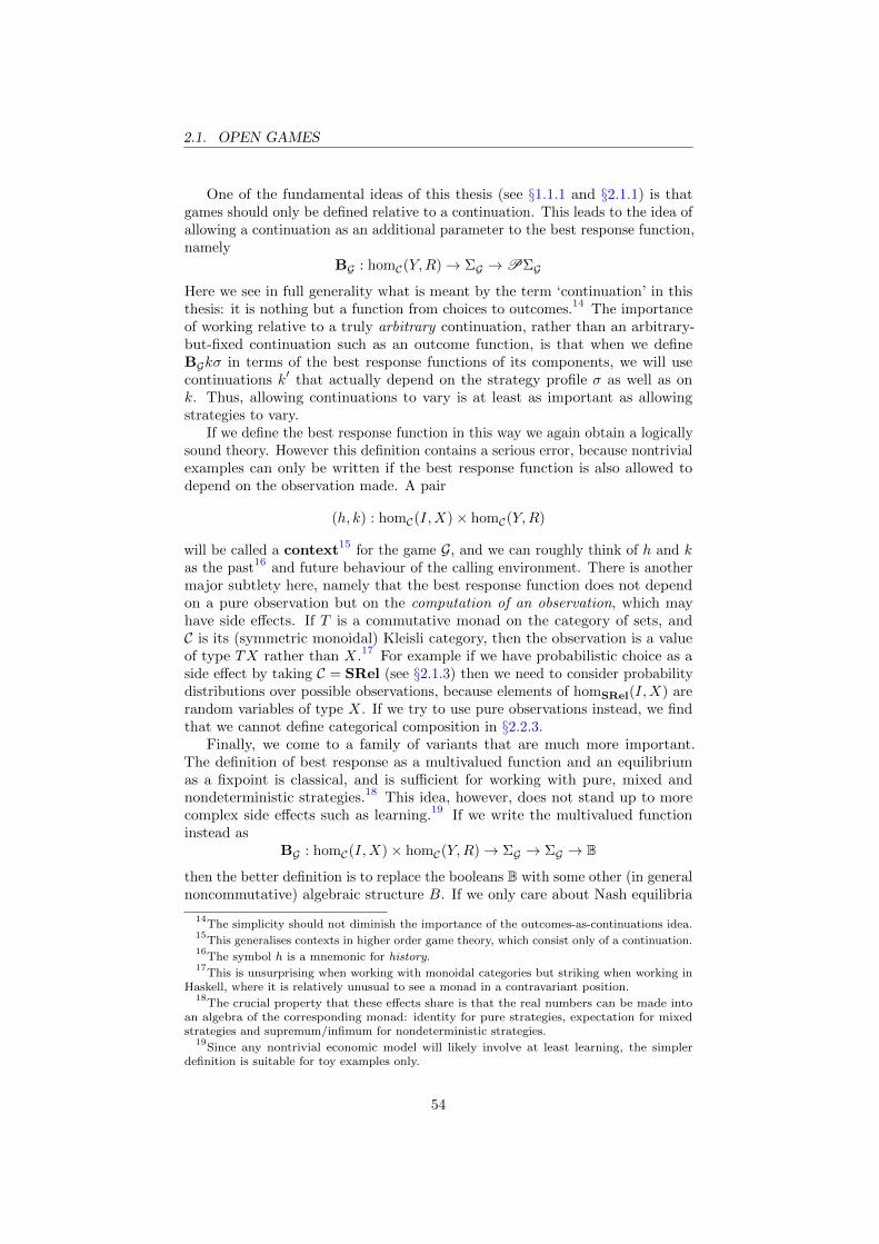
2.1. OPEN GAMES
One of the fundamental ideas of this thesis (see §1.1.1 and §2.1.1) is thatgames should only be defined relative to a continuation. This leads to the idea ofallowing a continuation as an additional parameter to the best response function,namely
BG : homC(Y,R)→ ΣG →PΣG
Here we see in full generality what is meant by the term ‘continuation’ in thisthesis: it is nothing but a function from choices to outcomes.14 The importanceof working relative to a truly arbitrary continuation, rather than an arbitrary-but-fixed continuation such as an outcome function, is that when we defineBGkσ in terms of the best response functions of its components, we will usecontinuations k′ that actually depend on the strategy profile σ as well as onk. Thus, allowing continuations to vary is at least as important as allowingstrategies to vary.
If we define the best response function in this way we again obtain a logicallysound theory. However this definition contains a serious error, because nontrivialexamples can only be written if the best response function is also allowed todepend on the observation made. A pair
(h, k) : homC(I,X)× homC(Y,R)
will be called a context15 for the game G, and we can roughly think of h and kas the past16 and future behaviour of the calling environment. There is anothermajor subtlety here, namely that the best response function does not dependon a pure observation but on the computation of an observation, which mayhave side effects. If T is a commutative monad on the category of sets, andC is its (symmetric monoidal) Kleisli category, then the observation is a valueof type TX rather than X.17 For example if we have probabilistic choice as aside effect by taking C = SRel (see §2.1.3) then we need to consider probabilitydistributions over possible observations, because elements of homSRel(I,X) arerandom variables of type X. If we try to use pure observations instead, we findthat we cannot define categorical composition in §2.2.3.
Finally, we come to a family of variants that are much more important.The definition of best response as a multivalued function and an equilibriumas a fixpoint is classical, and is sufficient for working with pure, mixed andnondeterministic strategies.18 This idea, however, does not stand up to morecomplex side effects such as learning.19 If we write the multivalued functioninstead as
BG : homC(I,X)× homC(Y,R)→ ΣG → ΣG → B
then the better definition is to replace the booleans B with some other (in generalnoncommutative) algebraic structure B. If we only care about Nash equilibria
14The simplicity should not diminish the importance of the outcomes-as-continuations idea.
15This generalises contexts in higher order game theory, which consist only of a continuation.
16The symbol h is a mnemonic for history.
17This is unsurprising when working with monoidal categories but striking when working in
Haskell, where it is relatively unusual to see a monad in a contravariant position.18
The crucial property that these effects share is that the real numbers can be made intoan algebra of the corresponding monad: identity for pure strategies, expectation for mixedstrategies and supremum/infimum for nondeterministic strategies.
19Since any nontrivial economic model will likely involve at least learning, the simpler
definition is suitable for toy examples only.
54

2.1. OPEN GAMES
then we can take B to be a monoid, however for reasoning about subgameperfection it seems that B should be some kind of ‘noncommutative completesemilattice’. A typical example would be of the form B = T ′B, where T ′ isanother (strong, not necessarily commutative) monad on the category of sets,which can be different to T , the monad with C = Kl(T ).20 Since it is still unclearwhat the appropriate definition should be we will use the simpler one by default.
2.1.6 Closed games
The reason for the terminology open game introduced in §2.1.4 is that an opengame is open to its environment, in the sense that information can pass back andforth. However, if one of X,Y,R, S in G : (X,S)→ (Y,R) is equal to the tensorunit I in C, then the flow of information is restricted, and if all are equal to Ithen no information can pass between the game and its environment. A closedgame is therefore defined21 to be an open game of type G : (I, I)→ (I, I).
Looking ahead to the result in §2.2.10, that open games are morphisms of amonoidal category whose objects are pairs of sets, and whose tensor unit is (I, I),a closed game can equivalently be called an abstract scalar. This terminologyis from [AC04, Abr05], and we will use it interchangeably with ‘closed game’.See also [KL80].
Closed games are particularly interesting when I is terminal in C. Thecategories Set and SRel both have this property, although Rel (which modelsnondeterminism) does not. In this case, closed games have a very simpleformulation: the play and coplay functions become trivial, and the game isdescribed entirely by its set ΣG of strategy profiles, and its best responsefunction, whose type reduces to
BG : ΣG →PΣG
A game in the intuitive, informal sense can be described by this data (see §1.2.4),and correspondingly there is no notion of information being shared with theenvironment in classical game theory, which suggests that games in the usualsense should be thought of as closed games.
A closed game G over any category has a canonical history and a canonicalcontinuation, namely both being given by idI . Thus we can give a solutionconcept for closed games: an equilibrium of G is a strategy profile σ : ΣG withσ ∈ BG(idI , idI)σ. This solution concept will be used in §3.1 and §3.2, wherewe see that it includes pure and mixed Nash and subgame perfect equilibria asspecial cases.
2.1.7 Decisions
In this section we see our first examples of open games, the decisions22, whichare one-player games. Every nontrivial game contains decisions as components,representing the players of the game.
20We can think of T as the effects allowed by the players, such as learning, and T
′as the
effects allowed by the economist, such as choosing a prior.21
Games are not doors, or topologies: every closed game is open, although it is reasonableto think of closed games as a degenerate case of open games.
22This term comes from decision theory, which mathematically is the study of one-player
games, but in practice is the applied study of modelling issues that are logically prior to gametheory.
55
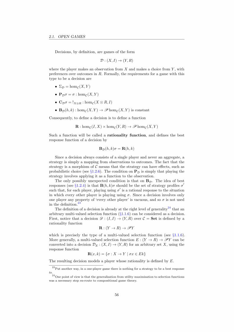
2.1. OPEN GAMES
Decisions, by definition, are games of the form
D : (X, I)→ (Y,R)
where the player makes an observation from X and makes a choice from Y , withpreferences over outcomes in R. Formally, the requirements for a game with thistype to be a decision are
• ΣD = homC(X,Y )
• PDσ = σ : homC(X,Y )
• CDσ = !X⊗R : homC(X ⊗R, I)
• BD(h, k) : homC(X,Y )→P homC(X,Y ) is constant
Consequently, to define a decision is to define a function
R : homC(I,X)× homC(Y,R)→P homC(X,Y )
Such a function will be called a rationality function, and defines the bestresponse function of a decision by
BD(h, k)σ = R(h, k)
Since a decision always consists of a single player and never an aggregate, astrategy is simply a mapping from observations to outcomes. The fact that thestrategy is a morphism of C means that the strategy can have effects, such asprobabilistic choice (see §1.2.6). The condition on PD is simply that playing thestrategy involves applying it as a function to the observation.
The only possibly unexpected condition is that on BD. The idea of bestresponses (see §1.2.4) is that B(h, k)σ should be the set of strategy profiles σ′
such that, for each player, playing using σ′ is a rational response to the situationin which every other player is playing using σ. Since a decision involves onlyone player any property of ‘every other player’ is vacuous, and so σ is not usedin the definition.23
The definition of a decision is already at the right level of generality24 that anarbitrary multi-valued selection function (§1.1.6) can be considered as a decision.First, notice that a decision D : (I, I) → (Y,R) over C = Set is defined by arationality function
R : (Y → R)→PY
which is precisely the type of a multi-valued selection function (see §1.1.6).More generally, a multi-valued selection function E : (Y → R)→PY can beconverted into a decision DE : (X, I)→ (Y,R) for an arbitrary set X, using theresponse function
R(x, k) = {σ : X → Y | σx ∈ Ek}
The resulting decision models a player whose rationality is defined by E.
23Put another way, in a one-player game there is nothing for a strategy to be a best response
to.24
One point of view is that the generalisation from utility maximisation to selection functionswas a necessary step en-route to compositional game theory.
56

2.1. OPEN GAMES
2.1.8 Preliminary examples of decisions
We will give two example families of decisions representing classically rationalplayers, respectively with pure and mixed strategies. In the first case, we takeC = Set. We will fix a rational preference relation25 � on a set R, representinga player’s preferences for different outcomes in R, where r � r′ means that theoutcome r is considered at least as good as the outcome r′. We will also fix anarbitrary set X and a finite set Y . To define a decision
D : (X, 1)→ (Y,R)
is to define a rationality function
R : X × (Y → R)→P(X → Y )
We define a particular family of decisions by the response functions
R(x, k) = {σ : X → Y | k(σx) � ky for all y : Y }
We will now explicitly give the data defining D. Its strategies are ΣD = X → Y ,and its play function PD : (X → Y ) → (X → Y ) is PDσx = σx. Its coplayfunction CD : (X → Y )→ (X ×R→ 1) is CD(σ, (x, r)) = ∗. Its best responsefunction
BD : X × (Y → R)→ (X → Y )→P(X → Y )
is given by
BD(x, k)σ = {σ′ : X → Y | k(σ′x) � ky for all y : Y }
For our second family of examples we will use C = SRel (defined in §2.1.3).For an arbitrary set X and finite set Y we define a decision
D : (X, 1)→ (Y,R)
modelling a player who maximises expected utility (see §1.2.6). To specify sucha decision is to specify a response function
R : DX × (Y → DR)→P(X → DY )
where D is the distribution monad (see §2.1.3). We use the particular function
R(h, k) = {σ : X → DY | E[k∗(σ∗h)] ≥ E[ky] for all y : Y }
where E : DR→ R is the expectation operator defined by
E[α] =∑
x∈supp(α)
P [α = x] · x
and −∗ is the Kleisli extension of D . Explicitly, we have the strategy setΣD = X → DY . The play function
PD : (X → DY )→ (X → DY )
25Recall that a rational preference relation is a total preorder, that is, a total order in which
we may have r 6= r′
with r � r′
and r′ � r. Thus � can be viewed as a total order on
equivalence classes.
57

2.1. OPEN GAMES
is given by P [PDσx = y] = P [σx = y]. The coplay function
CD : (X → DY )→ (X × R→ D1)
is given by P [CDσ(x, r) = ∗] = 1. The best response function
BD : DX × (Y → DR)→ (X → DY )→P(X → DY )
is given by
BD(h, k)σ = {σ′ : X → DY | E[k∗(σ′∗h)] ≥ E[ky] for all y : Y }
2.1.9 Computations and counit
Besides decisions, the other atomic games we will consider are computationsand counits. These components are unable to make strategic decisions, andin particular only have one strategy, which behaves trivially. Their purpose,however, is to control the information flow in a game. Examples of computationsinclude outcome functions, identities, copying and deleting. The counits serve toconnect forward-flowing to backward-flowing data, that is, identifying a particularforward-flowing value as the value that some player is reasoning about.
Formally, a computation is a game
(f, g) : (X,S)→ (Y,R)
defined by morphisms f : homC(X,Y ) and g : homC(R,S). After we have defineda symmetric monoidal category of games in §2.2.10, this will give us a symmetricmonoidal embedding of C × Cop (see §2.2.12). The definition is given by
• Σ(f,g) = 1 = {∗}
• P(f,g)∗ = f : homC(X,Y )
• C(f,g)∗ : homC(X ⊗R,S) is given by the composition
X ⊗R π2−→ Rg−→ S
• B(f,g)(h, k)∗ = {∗} for all h and k
The conditions Σ(f,g) = 1 and B(f,g)(h, k)∗ = {∗} implement the idea that (f, g)is ‘strategically trivial’. The fact that ∗ ∈ B(f,g)(h, k)∗ means that ∗ is alwaysan equilibrium of a computation. The idea behind this is that a strategy for anaggregate game should never fail to be an equilibrium because of a computation,because a computation has no preferences. Rather, if a strategy fails to be anequilibrium, it should always be because some player has incentive to deviate.We expand on this idea in §2.2.11.
The conditions on P(f,g) and C(f,g) determine the information flow, whichis explained in more detail in §2.2.14. When C = Set, the coplay function of acomputation is simply
C(f,g)∗(x, r) = gr
Next, for each object X of C we define a counit εX : (X,X)→ (I, I) by
• ΣεX = 1 = {∗}
58

2.2. THE CATEGORY OF GAMES
• PεX∗ = !X : homC(X, I)
• CεX∗ = ρX : homC(X ⊗ I,X)
• BεX(h, k)∗ = {∗} for all h and k
The intuition behind this definition is similar to that for computations. IfC = Set, the coplay function is CεX
∗(x, ∗) = x. Counits will not play a majorrole in this thesis, although see §2.2.13 and §2.3.6.
2.2 The category of games
2.2.1 Discussion
In §2.1 we introduced many definitions, especially of open games (§2.1.4), de-cisions (§2.1.7), computations and counits (§2.1.9). In this section we will addalgebraic structure, giving two ways to compose games: categorical composition,which is a primitive form of sequential play of games, and tensor product, whichis a primitive form of simultaneous play.
As a matter of fact, in this section we define two different categorical compo-sition operators. This is essentially a historical accident, and the state of affairsis discussed in the conclusion. These two categorical composition operatorsare called N -composition and SP -composition, and they correspond roughlyto a choice of solution concept between Nash equilibrium and subgame perfectequilibrium.
In this section we will additionally prove that N -composition and tensorproduct together obey the axioms of a symmetric monoidal category. In §2.3this algebraic structure will be investigated further. The appendix, whichclosely follows this section (minus the explanatory text) does the same for SP -composition, proving that it forms a symmetric premonoidal category with thesame definition of tensor product. Both operators will be used in chapter 3.
Readers who are not category theorists can treat composition and tensorproduct as rather like sequential and parallel composition operators in processalgebra26, similar to those in [BW13], with the axioms we check simply beingtechnical conditions for the string diagram language introduced in §2.3.5 to besound.
One important direction that we will not consider in this thesis (although it isdiscussed in the appendix) is to additionally consider morphisms between games,so that we have a monoidal bicategory [SP09]. This would allow us to give somecanonicity to the operators defined in this section (for example, characterisingthem as universal properties), and more importantly, when considering infinitegames such as repeated games, a natural approach is to define the game as aterminal coalgebra of a functor which precomposes a finite approximation tothe repeated game with one additional stage. Because a terminal coalgebra isdefined by a universal property of objects, this requires morphisms betweengames. There are several possible definitions that could be used, however, andat the present time it is not clear which are useful.27 One possibility that would
26An earlier, failed attempt at a compositional game theory by the author took this as a
starting point and used series-parallel partial orders [BdGR05] as part of the data specifying agame.
27Neil Ghani is currently working on this problem.
59
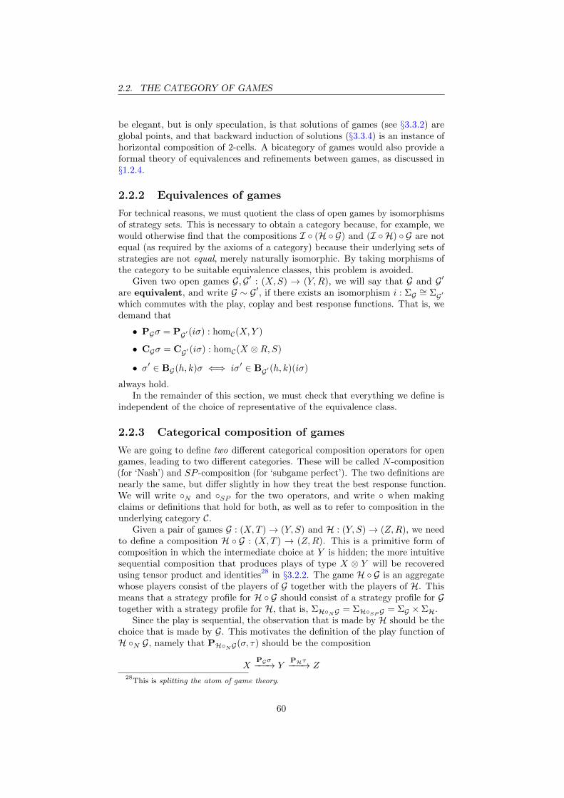
2.2. THE CATEGORY OF GAMES
be elegant, but is only speculation, is that solutions of games (see §3.3.2) areglobal points, and that backward induction of solutions (§3.3.4) is an instance ofhorizontal composition of 2-cells. A bicategory of games would also provide aformal theory of equivalences and refinements between games, as discussed in§1.2.4.
2.2.2 Equivalences of games
For technical reasons, we must quotient the class of open games by isomorphismsof strategy sets. This is necessary to obtain a category because, for example, wewould otherwise find that the compositions I ◦ (H ◦ G) and (I ◦ H) ◦ G are notequal (as required by the axioms of a category) because their underlying sets ofstrategies are not equal, merely naturally isomorphic. By taking morphisms ofthe category to be suitable equivalence classes, this problem is avoided.
Given two open games G,G′ : (X,S) → (Y,R), we will say that G and G′are equivalent, and write G ∼ G′, if there exists an isomorphism i : ΣG ∼= ΣG′
which commutes with the play, coplay and best response functions. That is, wedemand that
• PGσ = PG′(iσ) : homC(X,Y )
• CGσ = CG′(iσ) : homC(X ⊗R,S)
• σ′ ∈ BG(h, k)σ ⇐⇒ iσ′ ∈ BG′(h, k)(iσ)
always hold.In the remainder of this section, we must check that everything we define is
independent of the choice of representative of the equivalence class.
2.2.3 Categorical composition of games
We are going to define two different categorical composition operators for opengames, leading to two different categories. These will be called N -composition(for ‘Nash’) and SP -composition (for ‘subgame perfect’). The two definitions arenearly the same, but differ slightly in how they treat the best response function.We will write ◦N and ◦SP for the two operators, and write ◦ when makingclaims or definitions that hold for both, as well as to refer to composition in theunderlying category C.
Given a pair of games G : (X,T )→ (Y, S) and H : (Y, S)→ (Z,R), we needto define a composition H ◦ G : (X,T ) → (Z,R). This is a primitive form ofcomposition in which the intermediate choice at Y is hidden; the more intuitivesequential composition that produces plays of type X ⊗ Y will be recoveredusing tensor product and identities28 in §3.2.2. The game H ◦ G is an aggregatewhose players consist of the players of G together with the players of H. Thismeans that a strategy profile for H ◦ G should consist of a strategy profile for Gtogether with a strategy profile for H, that is, ΣH◦NG = ΣH◦SPG = ΣG × ΣH.
Since the play is sequential, the observation that is made by H should be thechoice that is made by G. This motivates the definition of the play function ofH ◦N G, namely that PH◦NG(σ, τ) should be the composition
XPGσ−−−→ Y
PHτ−−−→ Z28
This is splitting the atom of game theory.
60

2.2. THE CATEGORY OF GAMES
To be clear, this notation means that we have defined
PH◦NG(σ, τ) = PH◦SPG(σ, τ) = PHτ ◦PGσ
Using the categorical composition in C appropriately sequences the effects thatcan be used by the two components. For example if G and H both containplayers who can make probabilistic choices, the play function of H ◦ G gives theappropriate probability distribution on Z taking into account the probabilitydistribution on Y .
The coplay function of H ◦ G, on the other hand, is hard or impossible tojustify on intuitive grounds. We define CH◦G(σ, τ) to be the composition
X ⊗R ∆X⊗R−−−−→ X ⊗X ⊗RX⊗PGσ⊗R−−−−−−−→ X ⊗ Y ⊗R X⊗CHτ−−−−−→ X ⊗ S
CGσ−−−→ T
(where we are assuming that C is strict monoidal). When C = Set, this is givenexplicitly by
CH◦G(σ, τ)(x, r) = CGσ(x,CHτ(PGσx, r))
This will be discussed in §2.2.14.The two (different) cases for the best response function will be given without
for now, but will be discussed in detail in the next section. The definition forN -composition is
BH◦NG(h, k)(σ, τ) = BG(h, kτσ)×BH(PGσ ◦ h, k)τ
and that for SP -composition is
BH◦G(h, k)(σ, τ) = BG(h, kτ◦)σ ×⋂σ′:ΣG
BH(PGσ′ ◦ h, k)τ
In both cases, kτ◦ is the composition
Y∆Y−−→ Y ⊗ Y Y⊗PHτ−−−−−→ Y ⊗ Z Y⊗k−−−→ Y ⊗R CHτ−−−→ S
Notice that because σ is in the set ranged over by σ′, trivially BH◦SPG(h, k)(σ, τ)is a subset of BH◦NG(h, k)(σ, τ).
With these two definitions of composition, we obtain a categories GameN (C)and GameSP (C). For both categories the objects are pairs of objects of C,morphisms are equivalence classes of open games, and the identity on (X,R) isthe computation (idX , idR). The categories differ only in how composition isdefined. The axioms of a category, in both cases, will be proved in §2.2.5 and§2.2.6.
We must now prove that H ◦N G and H ◦SP G are well-defined, i.e. if G ∼ G′and H ∼ H′ then H ◦N G ∼ H
′ ◦N G′ and H ◦SP G ∼ H
′ ◦SP G′. We are
given isomorphisms iG : ΣG → ΣG′ and iH : ΣH → ΣH′ , and we define a newisomorphism iH◦NG(σ1, σ2) = (iGσ1, iHσ2). For the play function,
PH◦G(σ, τ) = PHτ ◦PGσ
= PH′(iHτ) ◦PG′(iGσ)
= PH′◦NG′(iH◦NG(σ, τ))
61

2.2. THE CATEGORY OF GAMES
Similarly for coplay,
CH◦G(σ, τ) = CGσ ◦ (X ⊗CHτ) ◦ (X ⊗PGσ ⊗R) ◦ (∆X ⊗R)
= CG′(iGσ) ◦ (X ⊗CH′(iHτ)) ◦ (X ⊗PG′(iGσ)⊗R) ◦ (∆X ⊗R)
= CH′◦NG′(iH◦NG(σ, τ))
For the best response functions, we first check that
kτ◦ = CHτ ◦ (Y ⊗ k) ◦ (Y ⊗PHτ) ◦∆Y
= CH′(iHτ) ◦ (Y ⊗ k) ◦ (Y ⊗PH′(iHτ)) ◦∆Y
= kiHτ◦
For N -composition, we have
BH◦NG(h, k)(σ, τ) = BG(h, kτ◦)σ ×BH(PGσ ◦ h, k)τ
and
BH′◦NG′(h, k)(iGσ, iHτ) = BG′(h, kiHτ◦)(iGσ)×BH′(PG′(iGσ) ◦ h, k)(iHτ)
Because kτ◦ = kiHτ◦ we immediately get BG(h, kτ◦)σ = BG′(h, kiHτ◦)(iGσ).Similarly, since PGσ ◦ h = PG′(iGσ) ◦ h, we also have
BH(PGσ ◦ h, k)τ = BH′(PG′(iGσ) ◦ h, k)(iHτ)
and we are done.For SP -composition, we have
BH◦SPG(h, k)(σ, τ) = BG(h, kτ◦)σ ×⋂σ′:ΣG
BH(PGσ′ ◦ h, k)τ
and
BH′◦SPG′(h, k)(iGσ, iHτ) = BG′(h, kiHτ◦)(iGσ)×
⋂σ′:ΣG′
BH′(PG′σ′ ◦ h, k)(iHτ)
The first terms are equal as previously. For the second part, take some
τ ′ ∈⋂σ′:ΣG
BH(PGσ′′ ◦ h, k)τ
Then for each σ′ : ΣG′ we have
τ ′ ∈ BH(PG(i−1G σ′′) ◦ h, k)τ
and henceiHτ
′ ∈ BH′(PG′σ′′ ◦ h, k)(iHτ)
The converse is symmetrical.
62

2.2. THE CATEGORY OF GAMES
2.2.4 Best response for sequential compositions
In order to give a definition of BH◦NG(h, k)(σ, τ), we need to define what it
means for a strategy profile (σ′, τ ′) to be a best response to (σ, τ), in the contextconsisting of a history h : homC(I,X) and a continuation k : homC(Z,R).
The idea is that we have a fixed situation in which the strategy profile playedis (σ, τ), and then one player unilaterally deviates to a component of σ′ or τ ′.This means that if we have a player in G deviating to a component of σ′ weknow that every player in H is playing τ , and vice versa.
The first condition is that σ′ should be a best response to σ, in a modifiedcontext in which we extend the continuation k backwards in time using the factthat we know that H will be played using τ . Therefore we define29 the extendedcontinuation kτ◦ to be the composition
Y∆Y−−→ Y ⊗ Y Y⊗PHτ−−−−−→ Y ⊗ Z Y⊗k−−−→ Y ⊗R CHτ−−−→ S
For the second condition we need that τ ′ is a best response to τ in anappropriate context. The same continuation k can be used without modification,and the history can be extended forwards using the fact that G will be playedwith σ, namely as the composition
Ih−→ X
PGσ−−−→ Y
This leads to the definition
BH◦NG(h, k)(σ, τ) =
{(σ′, τ ′) : ΣG × ΣH
∣∣∣∣ σ′ ∈ BG(h, kτ◦)σ andτ ′ ∈ BH(PGσ ◦ h, k)τ
}which can be written equivalently as
BH◦NG(h, k)(σ, τ) = BG(h, kτ◦)σ ×BH(PGσ ◦ h, k)τ
This is precisely the definition of N -composition.Assuming that when a player in H is deviating to τ ′, the players in G
use σ, leads to a theory of games supporting a solution concept based on Nashequilibrium. However our games are dynamic (that is to say, they have non-trivialtemporal structure in which players can observe events that happened in thepast), and it is widely recognised in game theory30 that Nash equilibrium is not asuitable solution concept for dynamic games. In particular, in a Nash equilibriumearlier players can make so-called ‘non-credible threats’ to later players. Thecategory GameN (C) behaves in this way, in that it allows strategies makingnon-credible threats to be equilibria (that is, fixpoints of the best responsefunction).
The usual solution to this problem is to use subgame-perfect equilibria (see§1.3.5). This is an equilibrium refinement of Nash: every subgame-perfectequilibrium is a Nash equilibrium, but not vice versa.31 In classical game theory,
29This is the only place in which the coplay function is actually used. All of the machinery
and the difficult interpretation of coplay begins with the fact that a function of the appropriatetype is needed here.
30This hardly needs a reference, but see for example [LBS08].
31In particular, the Nash equilibria which are not subgame-perfect are precisely the ones
containing non-credible threats.
63

2.2. THE CATEGORY OF GAMES
the usual method is to define ‘subgames’ as subtrees of the game tree, and definea subgame-perfect equilibrium to be a strategy which induces a Nash equilibriumwhen restricted to any subgame.
One possibility, therefore, would be to extend the data specifying a gamewith a recursively-built collection of subgames, and quantify over this collectionwhen defining the best-response function. However, a simpler solution is possible.An apparent alternative would be to quantify over the type of histories, and saythat a best response should be valid for every possible history, not just the onesthat arise from the strategy profile. For classical game theory this works32, butfor us it is too strong. Consider, for example, a game defined (over the categoryof sets, for simplicity) as a composition of the form
(X, I)(∆X ,idI)−−−−−−→ (X ⊗X, I)
D−→ (Y,R)
where D is a decision. Now the earlier component does not contain a playerand cannot make strategic decisions, so our intuition about threats is no longervalid. No matter what the starting history is, and no matter what this gameis precomposed with, the player making the decisions can only ever observehistories of the form (x, x). It is therefore too strong to require that the player’sstrategy should be rational for histories not of this form.
This example, however, suggests the solution: the image of the play function,as the strategy profile of the first component varies, gives precisely those historiesfor the second component that can possibly arise. Now we can return to theoriginal problem: defining what it means for (σ′, τ ′) to be a best response to(σ, τ) in the context (h, k). The second condition becomes that τ ′ should be abest response to τ now in a variety of contexts: all those of the form (h′, k),where h′ is of the form PGσ
′′ ◦ h, where σ′′ is an arbitrary strategy profilefor G. Putting this together and rewriting it, we get the stated definition ofSP -composition,
BH◦SPG(h, k)(σ, τ) = BG(h, kτ◦)σ ×⋂σ′:ΣG
BH(PGσ′ ◦ h, k)τ
The reason that we retain both definitions, rather than considering onlySP -composition, is that N -composition is better behaved with respect to thetensor operation that we will define later in this section.
2.2.5 The identity laws
We will now prove that GameN (C) and GameSP (C), as defined in §2.2.3, areboth categories, beginning with the identity laws. Let G : (X,S)→ (Y,R) be agame. We first prove that (idY , idR) ◦ G ∼ G for both N - and SP -composition,and hence they are equal after quotienting. Again, we use ◦ to refer to both ◦Nand ◦SP for the proof cases in which they are identical.
For the strategy sets,
Σ(idY , idR)◦G = ΣG × Σ(idY , idR) = ΣG × 1
32In classical game theory a ‘history’ can be defined as a path starting at the root of the
game tree, and such paths are in bijection with subtrees.
64

2.2. THE CATEGORY OF GAMES
and so we take the isomorphism i : ΣG × 1→ ΣG . For the play function,
P(idY , idR)◦G(iσ) = P(idY , idR)∗ ◦PGσ = idY ◦PGσ = PGσ
For coplay, by definition C(idY , idR)◦G(iσ) is the composition
X ⊗R ∆X⊗R−−−−→ X ⊗X ⊗RX⊗PGσ⊗R−−−−−−−→ X ⊗ Y ⊗R
X⊗C(idY , idR)∗−−−−−−−−−−→ X ⊗RCGσ−−−→ S
which, expanding the definitions further, is
X ⊗R ∆X⊗R−−−−→ X ⊗X ⊗RX⊗PGσ⊗R−−−−−−−→ X ⊗ Y ⊗R X⊗π2−−−−→ X ⊗R
CGσ−−−→ S
The first part of this is the identity on X ⊗R, so it is equal to CGσ.For best response with N -composition,
iσ′ ∈ B(idY ,idR)◦NG(h, k)(iσ)
⇐⇒ (σ′, ∗) ∈ BG(h, k∗◦)σ ×B(idY ,idR)(PG(iσ) ◦ h, k)∗⇐⇒ σ′ ∈ BG(h, k∗◦)σ
The continuation k∗◦ is given by
Y∆Y−−→ Y ⊗ Y
Y⊗P(idY , idR)∗−−−−−−−−−−→ Y ⊗ Y Y⊗k−−−→ Y ⊗RC(idY , idR)∗−−−−−−−−→ R
Expanding the definitions and simplifying, this is
Y∆Y−−→ Y ⊗ Y Y⊗k−−−→ Y ⊗R π2−→ R
which is equal to k, and we are done. For SP -composition, instead we have
iσ′ ∈ B(idY ,idR)◦G(h, k)(iσ)
⇐⇒ (σ′, ∗) ∈ BG(h, k∗◦)σ ×⋂
σ′′
:ΣG
B(idY ,idR)(PGσ′′ ◦ h, k)∗
⇐⇒ σ′ ∈ BG(h, k∗◦)σ
and again k∗◦ = k.For the other identity law, we will prove that G ◦ (idX , idS) ∼ G. For the
strategy sets,
ΣG◦(idX , idS) = Σ(idX , idS) × ΣG = 1× ΣG ∼= ΣG
now with the isomorphism i : ΣG → 1× ΣG . For the play function,
PG◦(idX , idS)(iσ) = PGσ ◦P(idX , idS)∗ = PGσ ◦ idX = PGσ
For coplay we have that CG◦(idX , idS)(iσ) is the composition
X ⊗R ∆X⊗R−−−−→ X ⊗X ⊗RX⊗P(idX, idS)∗⊗R−−−−−−−−−−−−→ X ⊗X ⊗R
65

2.2. THE CATEGORY OF GAMES
X⊗CGσ−−−−−→ X ⊗ SC(idX, idS)∗−−−−−−−−→ S
Expanding and simplifying, this is
X ⊗R ∆X⊗R−−−−→ X ⊗X ⊗RX⊗CGσ−−−−−→ X ⊗ S π2−→ S
which is equal to CGσ.For best response with N -composition we have
iσ′ ∈ BG◦N (idX ,idS)(h, k)(iσ)
⇐⇒ (∗, σ′) ∈ B(idX ,idS)(h, kσ◦)∗ ×BG(P(idX ,idS)∗ ◦ h, k)σ
⇐⇒ σ′ ∈ BG(P(idX ,idS)∗ ◦ h, k)σ
⇐⇒ σ′ ∈ BG(h, k)σ
because P(idX ,idS)∗ = idX . On the other hand, for SP -composition,
iσ′ ∈ BG◦SP (idX ,idS)(h, k)(iσ)
⇐⇒ (∗, σ′) ∈ B(idX ,idS)(h, kσ◦)∗ ×⋂
σ′′
:Σ(idX,idS)
BG(P(idX ,idS)σ′′ ◦ h, k)σ
⇐⇒ σ′ ∈ BG(P(idX ,idS)∗ ◦ h, k)σ
⇐⇒ σ′ ∈ BG(h, k)σ
In summary, we have proved that the identity for composition on an object(X,R) is (idX , idR), in both categories GameN (C) and GameSP (C).
2.2.6 Associativity
Consider games
(W,U)G−→ (X,T )
H−→ (Y, S)I−→ (Z,R)
We will prove thatI ◦ (H ◦ G) ∼ (I ◦ H) ◦ G
for both N -composition and SP -composition. For SP -composition especially,this associativity law is not obvious.
The two sets of strategy profiles are ΣI◦(H◦G) = (ΣG × ΣH) × ΣI andΣ(I◦H)◦G = ΣG × (ΣH × ΣI), so we take the isomorphism
i : (ΣG × ΣH)× ΣI → ΣG × (ΣH × ΣI)
The case for the play function follows immediately from associativity ofcomposition in the underlying category C:
PI◦(H◦G)((σ, τ), υ) = PIυ ◦PH◦G(σ, τ)
= PIυ ◦PHτ ◦PGσ
= PI◦H(τ, υ) ◦PGσ
= P(I◦H)◦G(i((σ, τ), υ))
66

2.2. THE CATEGORY OF GAMES
For coplay, by definition CI◦(H◦G)((σ, τ), υ) is the composition
W ⊗R ∆W⊗R−−−−−→W ⊗W ⊗RW⊗PH◦G(σ,τ)⊗R−−−−−−−−−−−−→W ⊗ Y ⊗R
W⊗CIυ−−−−−→W ⊗ SCH◦G(σ,τ)−−−−−−−→ U
which is
W ⊗R ∆W⊗R−−−−−→W ⊗W ⊗RW⊗PGσ⊗R−−−−−−−−→W ⊗X ⊗R
W⊗PHτ⊗R−−−−−−−−→W ⊗ Y ⊗R W⊗CIυ−−−−−→W ⊗ S ∆W⊗S−−−−−→W ⊗W ⊗ SW⊗PGσ⊗S−−−−−−−→W ⊗X ⊗ S W⊗CHτ−−−−−−→W ⊗ T
CGσ−−−→ U
On the other hand C(I◦H)◦G(i((σ, τ), υ)) is
W ⊗R ∆W⊗R−−−−−→W ⊗W ⊗RW⊗PGσ⊗R−−−−−−−−→W ⊗X ⊗R
W⊗CI◦H(τ,υ)−−−−−−−−−→W ⊗ TCGσ−−−→ U
which is
W ⊗R ∆W⊗R−−−−−→W ⊗W ⊗RW⊗PGσ⊗R−−−−−−−−→W ⊗X ⊗R
W⊗∆X⊗R−−−−−−−→W ⊗X ⊗X ⊗R W⊗X⊗PHτ⊗R−−−−−−−−−−→W ⊗X ⊗ Y ⊗RW⊗X⊗CIυ−−−−−−−−→W ⊗X ⊗ S W⊗CHτ−−−−−−→W ⊗ T CIσ−−−→ U
and these two morphisms are equal by the comonoid laws for ∆.33 For anotherperspective on this part of the proof, see §2.2.14.
For best response for N -composition, we have
((σ′, τ ′), υ′) ∈ BI◦N (H◦NG)(h, k)((σ, τ), υ)
⇐⇒ ((σ′, τ ′), υ′) ∈ BH◦NG(h, kυ◦)(σ, τ)×BI(PH◦NG(σ′′, τ ′′) ◦ h, k)υ
⇐⇒ (σ′, τ ′, υ′) ∈ BG(h, (kυ◦)τ◦)σ
×BH(PGσ ◦ h, kυ◦)τ ×BI(PHτ ◦PGσ ◦ h, k)υ
and
i((σ′, τ ′), υ′) ∈ B(I◦NH)◦NG(h, k)(i((σ, τ), υ))
⇐⇒ (σ′, (τ ′, υ′)) ∈ BG(h, k(τ,υ)◦)σ ×BI◦NH(PGσ ◦ h, k)(τ, υ)
⇐⇒ (σ′, τ ′, υ′) ∈ BG(h, k(τ,υ)◦)σ
×BH(PGσ ◦ h, kυ◦)τ ×BI(PHτ ◦PGσ ◦ h, k)υ
Here kυ◦ is the composition
Y∆Y−−→ Y ⊗ Y Y⊗PIυ−−−−−→ Y ⊗ Z Y⊗k−−−→ Y ⊗R CIυ−−−→ S
and (kυ◦)τ◦ is the composition
X∆X−−→ X ⊗X X⊗PHτ−−−−−→ X ⊗ Y X⊗kυ◦−−−−−→ X ⊗ S CHτ−−−→ T
33Since this is not a thesis on category theory, detailed proofs by diagram chasing will not
be included for assertions like this that a complicated pair of morphisms are equal.
67

2.2. THE CATEGORY OF GAMES
which expands to
X∆X−−→ X ⊗X X⊗PHτ−−−−−→ X ⊗ Y X⊗∆Y−−−−−→ X ⊗ Y ⊗ Y
X⊗Y⊗PIυ−−−−−−−→ X ⊗ Y ⊗ Z X⊗Y⊗k−−−−−→ X ⊗ Y ⊗R X⊗CIυ−−−−−→ X ⊗ S CHτ−−−→ T
On the other hand k(τ,υ)◦ is the composition
X∆X−−→ X ⊗X X⊗PI◦H(τ,υ)−−−−−−−−−→ X ⊗ Z X⊗k−−−→ X ⊗R CI◦H(τ,υ)−−−−−−−→ T
which expands to
X∆X−−→ X ⊗X X⊗PHτ−−−−−→ X ⊗ Y X⊗PIυ−−−−−→ X ⊗ Z X⊗k−−−→ X ⊗R
∆X⊗R−−−−→ X ⊗X ⊗R X⊗PHτ⊗R−−−−−−−−→ X ⊗ Y ⊗R PIυ−−−→ X ⊗ S PHτ−−−→ T
Then (kυ◦)τ◦ = k(τ,υ)◦, and we are done.For SP -composition, on the other hand, we have
((σ′, τ ′), υ′) ∈ BI◦SP (H◦SPG)(h, k)((σ, τ), υ)
⇐⇒ ((σ′, τ ′), υ′) ∈ BH◦SPG(h, kυ◦)(σ, τ)
×⋂
(σ′′,τ′′
):ΣH◦SP G
BI(PH◦SPG(σ′′, τ ′′) ◦ h, k)υ
⇐⇒ (σ′, τ ′, υ′) ∈ BG(h, (kυ◦)τ◦)σ
×⋂
σ′′
:ΣG
BH(PGσ′′ ◦ h, kυ◦)τ ×
⋂σ′′
:ΣGτ′′
:ΣH
BI(PHτ′′ ◦PGσ
′′ ◦ h, k)υ
and
i((σ′, τ ′), υ′) ∈ B(I◦SPH)◦SPG(h, k)(i((σ, τ), υ))
⇐⇒ (σ′, (τ ′, υ′)) ∈ BG(h, k(τ,υ)◦)σ ×⋂
σ′′
:ΣG
BI◦SPH(PGσ′′ ◦ h, k)(τ, υ)
⇐⇒ (σ′, (τ ′, υ′)) ∈ BG(h, k(τ,υ)◦)σ
×⋂
σ′′
:ΣG
BH(PGσ′′ ◦ h, kυ◦)τ ×
⋂τ′′
:ΣH
BI(PHτ′′ ◦PGσ
′′ ◦ h, k)υ
⇐⇒ (σ′, τ ′, υ′) ∈ BG(h, k(τ,υ)◦)σ
×⋂
σ′′
:ΣG
BH(PGσ′′ ◦ h, kυ◦)τ ×
⋂σ′′
:ΣGτ′′
:ΣH
BI(PHτ′′ ◦PGσ
′′ ◦ h, k)υ
with the same continuations.
2.2.7 Tensor product of games
Besides the two variants of categorical composition introduced in §2.2.3, theother aggregation operator we will consider is a tensor (or monoidal) product.Given an arbitrary pair of games
G : (X1, S1)→ (Y1, R1)
68

2.2. THE CATEGORY OF GAMES
andH : (X2, S2)→ (Y2, R2)
we can form their tensor product
G ⊗H : (X1 ⊗X2, S1 ⊗ S2)→ (Y1 ⊗ Y2, R1 ⊗R2)
Since the tensor product ⊗ of C can be extended componentwise to pairsof objects, this will give us a product-like operator on both GameN (C) andGameSP (C), the categories defined in §2.2.3. Whereas both variants of H ◦ Gbehaves like the sequential play of G and H, the purpose of G ⊗H is to behavelike the simultaneous play.
Just as for sequential composition, a strategy profile for an aggregate of twogames consists of a strategy profile for each game, thus
ΣG⊗H = ΣG × ΣH
The play function can be defined using the tensor product of morphisms in C, by
PG⊗H(σ, τ) = PGσ ⊗PHτ
Similarly, the coplay function is
CG⊗H : ΣG × ΣH → homC(X1 ⊗X2 ⊗R1 ⊗R2, S1 ⊗ S2)
where CG⊗H(σ, τ) is given by
X1 ⊗X2 ⊗R1 ⊗R2
∼=−→ X1 ⊗R1 ⊗X2 ⊗R2
CGσ⊗CHτ−−−−−−−→ S1 ⊗ S2
To define the best response function
BG⊗H : homC(I,X1 ⊗X2)× homC(Y1 ⊗ Y2, R1 ⊗R2)→ ΣG × ΣH
→P(ΣG × ΣH)
essentially the same reasoning applies as in §2.2.4, except that we are nowworking with simultaneous games, and with selection equilibria (in the senseof §1.2.3), rather than subgame perfect equilibria. Given h : homC(I,X1 ⊗X2),we can take the canonical projections of it to form the component historiesh1 : homC(I,X1) and h2 : homC(I,X2). More importantly, given a continuationk : homC(Y1⊗Y2, R1⊗R2), a history h : homC(I,X1⊗X2) and a strategy profile(σ, τ) : ΣG × ΣH, we can form smaller continuations34 in which each componentmay deviate from the strategy, while the other stays fixed. The continuationfor the first player is denoted k⊗τ(h2) : homC(Y1, R1), and is defined by thecomposition
Y1
∼=−→ Y1 ⊗ IY1⊗h2−−−−→ Y1 ⊗X2
Y1⊗PHτ−−−−−−→ Y1 ⊗ Y2k−→ R1 ⊗R2
π1−→ R1
Similarly, the continuation kσ(h1)⊗ : homC(Y2, R2) for the second player is
Y2
∼=−→ I ⊗ Y2h1⊗Y2−−−−→ X1 ⊗ Y2
PGσ⊗Y2−−−−−→ Y1 ⊗ Y2k−→ R1 ⊗R2
π2−→ R2
34These are generalised forms of the unilateral continuations introduced in §1.2.2.
69

2.2. THE CATEGORY OF GAMES
Given these definitions, the best response function for the tensor product is givenby
BG⊗H(h, k)(σ, τ) = BG(h1, k⊗τ(h2))σ ×BH(h2, kσ(h1)⊗)τ
This definition will be refuted in §3.3.7, however.We will now prove that the tensor product is well-defined on equivalence
classes. Take equivalences G ∼ G′ and H ∼ H′, so we have isomorphismsiG : ΣG → ΣG′ and iH : ΣH → ΣH′ . We will prove that there is an equivalence
G ⊗ H ∼ G′ ⊗ H′ given by the isomorphism iG⊗H(σ, τ) = (iGσ, iHτ). For theplay function,
PG⊗H(σ, τ) = PGσ ⊗PHτ = PG′(iGσ)⊗PH′(iHτ) = PG′⊗H′(iG⊗H(σ, τ))
For coplay,
CG⊗H(σ, τ) = (CGσ ⊗CHτ) ◦ (X1 ⊗ sX2,R1⊗R2)
= (CG′(iGσ)⊗CH′(iHτ)) ◦ (X1 ⊗ sX2,R1⊗R2)
= CG′⊗H′(iG⊗H(σ, τ))
For best reponse, similarly to §2.2.3 we first check that there is an equalityof continuations
k⊗τ(h2) = π1 ◦ k ◦ (Y1 ⊗PHτ) ◦ (Y1 ⊗ h2) ◦ ρ−1Y1
= π1 ◦ k ◦ (Y1 ⊗PH′(iHτ)) ◦ (Y1 ⊗ h2) ◦ ρ−1Y1
= k⊗iHτ(h2)
and similarly kσ(h1)⊗ = kiGσ(h1)⊗. Then
iG⊗H(σ′, τ ′) ∈ BG′⊗H′(h, k)(iG⊗H(σ, τ))
⇐⇒ (iGσ′, iHτ
′) ∈ BG′(h1, k⊗iHτ(h2))(iGσ)×BH′(h2, kiGσ(h1)⊗)(iHτ)
⇐⇒ (σ′, τ ′) ∈ BG(h1, k⊗τ(h2))σ ×BH(h2, kσ(h1)⊗)τ
⇐⇒ (σ′, τ ′) ∈ BG⊗H(h, k)(σ, τ)
2.2.8 Functoriality of the tensor product
We will now prove that ⊗ makes GameN (C) into a symmetric monoidal category.We will also prove that on GameSP (C), ⊗ is only a premonoidal product [PR93],which is to say, all of the monoidal category axioms hold except that ⊗ is not abifunctor, but is only individually functorial in its two arguments.
The action of the monoidal product on objects (of both categories) is topairwise apply the monoidal product of C, so
(X1, R1)⊗ (X2, R2) = (X1 ⊗X2, R1 ⊗R2)
The action on morphisms, which are games, is exactly the construction givenin §2.2.7. The monoidal unit is (I, I), where I is the monoidal unit of C. Thesymmetric monoidal category axioms underly the string diagram language forGameN (C) introduced in §2.3.5 and used in the remainder of this thesis.
70

2.2. THE CATEGORY OF GAMES
We will first prove the identity law, which is the same for both GameN (C)and GameSP (C), namely
id(X1,R1) ⊗ id(X2,R2) ∼ id(X1⊗X2,R1⊗R2)
Since Σid(X1,R1)⊗id(X2,R2)= 1× 1 and Σid(X1⊗X2,R1⊗R2)
= 1, we take the isomor-
phism i(∗, ∗) = ∗. For the play function,
Pid(X1,R1)⊗id(X2,R2)(∗, ∗) = Pid(X1,R1)
∗ ⊗Pid(X2,R2)∗
= idX1⊗ idX2
= idX1⊗X2
= Pid(X1⊗X2,R1⊗R2)∗
For coplay,
Cid(X1,R1)⊗id(X2,R2)(∗, ∗)
= (Cid(X1,R1)∗ ⊗Cid(X2,R2)
∗) ◦ (X1 ⊗ sX2,R1⊗R2)
= ((idR1◦ πX1⊗X2→R1
)⊗ (idR2◦ πX2⊗R2→R2
)) ◦ (X1 ⊗ sX2,R1⊗R2)
= (idR1⊗ idR2
) ◦ (πX1⊗R1→R1⊗ πX2⊗R2→R2
) ◦ (X1 ⊗ sX2,R1⊗R2)
= idR1⊗R2◦ πX1⊗X2⊗R1⊗R2→R1⊗R2
= Cid(X1⊗X2,R1⊗R2)∗
where the canonical projections have been labelled with their types for clarity.For best response, we note that
∗ ∈ Bid(X1⊗X2,R1⊗R2)(h, k)∗
always holds, and so does
(∗, ∗) ∈ Bid(X1,R1)⊗id(X2,R2)(h, k)(∗, ∗)
= Bid(X1,R1)(h1, k⊗∗(h2))∗ ×Bid(X2,R2)
(h2, k∗(h1)⊗)∗
Now we come to the distributivity law of a bifunctor, namely
(H1 ◦ G1)⊗ (H2 ◦ G2) ∼ (H1 ⊗H2) ◦ (G1 ⊗ G2)
This is false for ◦SP , but the only case that fails is best response. We will firstgive the proof for ◦N . To prove distributivity of ◦N and ⊗, we have
Σ(H1◦NG1)⊗(H2◦NG2) = (ΣG1 × ΣH1)× (ΣG2 × ΣH2
)
andΣ(H1⊗H2)◦N (G1⊗G2) = (ΣG1 × ΣG2)× (ΣH1
× ΣH2)
and so we take the isomorphism i((σ1, τ1), (σ2, τ2)) = ((σ1, σ2), (τ1, τ2)). For theplay functions,
P(H1◦NG1)⊗(H2◦NG2)((σ1, τ1), (σ2, τ2)) = PH1◦NG1(σ1, τ1)⊗PH2◦NG2(σ2, τ2)
= (PH1τ1 ◦PG1σ1)⊗ (PH2
τ2 ◦PG2σ2)
= (PH1τ1 ⊗PH2
τ2) ◦ (PG1σ1 ⊗PG2σ2)
= PH1⊗H2(τ1, τ2) ◦PG1⊗G2(σ1, σ2)
= P(H1⊗H2)◦N (G1⊗G2)((σ1, σ2), (τ1, τ2))
71

2.2. THE CATEGORY OF GAMES
The proof for coplay would be extremely tedious to do in a similar style, butwe can instead prove it by drawing string diagrams in the symmetric monoidalcategory C [Sel11], and observing that one can be deformed into the other. Thestring diagram corresponding to C(H1◦NG1)⊗(H2◦NG2)((σ1, τ1), (σ2, τ2)) is
X1
X2
R1
R2
PG1σ1
PG2σ2
CH1τ1
CH2τ2
CG1σ1
CG2σ2
T1
T2
Y1
Y2
S1
S2
and for C((H1⊗H2)◦N (G1⊗G2))((σ1, σ2), (τ1, τ2)) is
X1
X2
R1
R2
PG1σ1
PG2σ2 CH1τ1
CH2τ2
CG1σ1
CG2σ2
T1
T2
Y1
Y2
S1
S2
72

2.2. THE CATEGORY OF GAMES
2.2.9 Functoriality of the tensor product, continued
We will first prove the remaining case of the distributivity law for ◦N , namelythat
((σ′1, τ′1), (σ′2, τ
′2)) ∈ B(H1◦NG1)⊗(H2◦NG2)(h, k)((σ1, τ1), (σ2, τ2))
is equivalent to
((σ′1, σ′2), (τ ′1, τ
′2)) ∈ B(H1⊗H2)◦N (G1⊗G2)(h, k)((σ1, σ2), (τ1, τ2))
We begin by expanding B(H1◦NG1)⊗(H2◦NG2)(h, k)((σ1, τ1), (σ2, τ2)) to
BH1◦NG1(h1, k⊗(σ2,τ2)(h2))(σ1, τ1)×BH2◦NG2(h2, k(σ1,τ1)(h1)⊗)(σ2, τ2)
The first term of this is
BG1(h1, (k⊗(σ2,τ2)(h2))τ1◦)σ1 ×BH1(PG1σ1 ◦ h1, k⊗(σ2,τ2)(h2))τ1
and the second is
BG2(h2, (k(σ1,τ1)(h1)⊗)τ2◦)σ2 ×BH2(PG2σ2 ◦ h2, k(σ1,τ1)(h1)⊗)τ2
The product of these can be written isomorphically as(BG1(h1, (k⊗(σ2,τ2)(h2))τ1◦)σ1 ×BG2(h2, (k(σ1,τ1)(h1)⊗)τ2◦)σ2
)×(BH1
(PG1σ1 ◦ h1, k⊗(σ2,τ2)(h2))τ1 ×BH2(PG2σ2 ◦ h2, k(σ1,τ1)(h1)⊗)τ2
)On the other hand, B(H1⊗H2)◦N (G1⊗G2)(h, k)((σ1, σ2), (τ1, τ2)) expands to
BG1⊗G2(h, k(τ1,τ2)◦)(σ1, σ2)×BH1⊗H2(PG1⊗G2(σ1, σ2) ◦ h, k)(τ1, τ2)
for which the first term is
BG1(h1, (k(τ1,τ2)◦)⊗σ2(h2))σ1 ×BG2(h2, (k(τ1,τ2)◦)σ1(h1)⊗)σ2
and the second is
BH1((PG1⊗G2(σ1, σ2) ◦ h)1, k⊗τ2((PG1⊗G2
(σ1,σ2)◦h)2))τ1
× BH2((PG1⊗G2(σ1, σ2) ◦ h)2, kτ1((PG1⊗G2
(σ1,σ2)◦h)1)⊗)τ2
Comparing these, it suffices to, firstly, have equalities of histories
PG1σ1 ◦ h1 = (PG1⊗G2(σ1, σ2) ◦ h)1
PG2σ2 ◦ h2 = (PG1⊗G2(σ1, σ2) ◦ h)2
which are both immediate consequences of the comonoid axioms, and secondlyto have equalities of continuations
(k⊗(σ2,τ2)(h2))τ1◦ = (k(τ1,τ2)◦)⊗σ2(h2)
(k(σ1,τ1)(h1)⊗)τ2◦ = (k(τ1,τ2)◦)σ1(h1)⊗
k⊗(σ2,τ2)(h2) = k⊗τ2(PG2σ2◦h2)
k(σ1,τ1)(h1)⊗ = kτ1(PG1σ1◦h1)⊗
73

2.2. THE CATEGORY OF GAMES
To prove these, again we draw string diagrams in C. The first equality is theequivalence between
Y1
PH1τ1
h
PG2σ2 PH2τ2
k
CH1τ1 S1Z1
X1
X2 Y2Z2
R1
R2
and
Y1
h
PG2σ2
PH1τ1
PH2τ2
k
CH1τ1
CH2τ2
S1
X1
X2
Y2
Z1
Z2
R1
R2
S2
The second is symmetrical to this. Both sides of the third are directly equal to
Z1∼= Z1 ⊗ I
Z2⊗h2−−−−→ Z1 ⊗X2
Z1⊗PG2σ2−−−−−−−→ Z1 ⊗ Y2
Z1⊗PH2τ2−−−−−−−→ Z1 ⊗ Z2
k−→ R1 ⊗R2π1−→ R1
and again the fourth is symmetrical.These third and fourth equalities of continuations are precisely what fails
if we use the definition of composition from §2.2.3 involving subgame-perfectequilibrium. In that case, one side uses only the strategy profile (σ1, σ2), butthe other side ranges over all deviations (σ′′1 , σ
′′2 ). With the other definition ⊗ is
still a premonoidal product [PR93], namely, it is individually functorial in thetwo entries, but is not a bifunctor. We will now prove this.
Since ◦N and ◦SP behave identically for strategy profiles, play and coplay,these cases follow directly from what was proved in the previous section, namelyby taking either G1 = H1 or G2 = H2 to both be an identity morphism. Thedistributivity laws for a premonoidal product are
(H ◦SP G)⊗ id(X′,R′) ∼ (H⊗ id(X
′,R′)) ◦SP (G ⊗ id(X
′,R′))
74

2.2. THE CATEGORY OF GAMES
andid(X
′,R′) ⊗ (H ◦SP G) ∼ (id(X
′,R′) ⊗H) ◦SP (id(X
′,R′) ⊗ G)
Because the definition of ⊗ is completely symmetrical, we will prove the case forbest response only for the first.
Given thatΣ(H◦SPG)⊗id
(X′,R′)
= (ΣG × ΣH)× 1
andΣ(H⊗id
(X′,R′))◦SP (G⊗id
(X′,R′)) = (ΣG × 1)× (ΣH × 1)
we take the isomorphism i((σ, τ), ∗) = ((σ, ∗), (τ, ∗)). We must show that
((σ′, τ ′), ∗) ∈ B(H◦SPG)⊗id(X′,R′)(h, k)((σ, τ), ∗)
is equivalent to
((σ′, ∗), (τ ′, ∗)) ∈ B(H⊗id(X′,R′))◦SP (G⊗id
(X′,R′))(h, k)((σ, ∗), (τ, ∗))
The former expands as
((σ′, τ ′), ∗) ∈ B(H◦SPG)⊗id(X′,R′)(h, k)((σ, τ), ∗)
⇐⇒ ((σ′, τ ′), ∗) ∈ BH◦SPG(h, k⊗∗(h2))(σ, τ)×Bid(X′,R′)(h2, k(σ,τ)(h1)⊗)∗
⇐⇒ (σ′, τ ′) ∈ BG(h1, (k⊗∗(h2))τ◦)σ ×⋂
σ′′
:ΣG
BH(PGσ′′ ◦ h1, k⊗∗(h2))τ
and the latter as
((σ′, ∗), (τ ′, ∗)) ∈ B(H⊗id(X′,R′))◦SP (G⊗id
(X′,R′))(h, k)((σ, ∗), (τ, ∗))
⇐⇒ ((σ′, ∗), (τ ′, ∗)) ∈ BG⊗id(X′,R′)(h, k(τ,∗)◦)(σ, ∗)
×⋂
(σ′′,∗):
ΣG×1
BH⊗id(X′,R′)(PG⊗id
(X′,R′)(σ′′, ∗) ◦ h, k)(τ, ∗)
⇐⇒ (σ′, τ ′) ∈ BG(h1, (k(τ,∗)◦)⊗∗(h2))σ
×⋂
σ′′
:ΣG
BH((PG⊗id(X′,R′)(σ′′, ∗) ◦ h)1, k⊗∗((PG⊗id
(X′,R′)(σ′′,∗)◦h)2))τ
The equalities
PGσ′′ ◦ h1 = (PG⊗id
(X′,R′)(σ′′, ∗) ◦ h)1
and(k⊗∗(h2))τ◦ = (k(τ,∗)◦)⊗∗(h2)
are special cases of the equivalents proved above for ◦N . The remaining equalityof continuations to be proved, namely
k⊗∗(h2) = k⊗∗((PG⊗id(X′,R′)(σ′′,∗)◦h)2)
also follows immediately from the equality of histories
h2 = (PG⊗id(X′,R′)(σ′′, ∗) ◦ h)2
This completes the proof.
75

2.2. THE CATEGORY OF GAMES
2.2.10 The monoidal category axioms
The remaining work in proving that GameN (C) is a monoidal category andGameSP (C) is a premonoidal category is to prove the monoidal category axioms.(To be clear, the axioms of a premonoidal category are still usually called the‘monoidal category axioms’ because they are identical to those of a monoidalcategory; the only difference in a premonoidal category is that ⊗ is not abifunctor.)
In general, proving these axioms takes a significant amount of work. Wemust define three families of morphisms, the left and right unitors and theassociators, prove their naturality, and then prove the commutativity of twodiagrams including the Mac Lane pentagon. To prove that a (pre-) monoidalcategory is symmetric we must additionally define the braiding morphisms,prove their naturality, and prove commutativity of an additional three diagrams.Fortunately, these structure morphisms and the proofs of the axioms are exactlyidentical in the two cases of GameN (C) and GameSP (C).
Most of this work can be avoided by appealing to Mac Lane’s coherencetheorem [Mac78] and replacing C with a monoidally equivalent strict monoidalcategory.35 In that case we have equalities of objects
(I, I)⊗ (X,R) = (I ⊗X, I ⊗R) = (X,R) = (X ⊗ I,R⊗ I) = (X,R)⊗ (I, I)
and so we can take all of the unitors to be the identity morphisms (that is,computations formed of pairs of identities, see §2.2.3), which are automaticallynatural and satisfy the commutative diagrams, simply by the fact that GameN (C)and GameSP (C) are categories. Similarly we have equalities
((X1, R1)⊗ (X2, R2))⊗ (X3, R3) = (X1 ⊗X2 ⊗X3, R1 ⊗R2 ⊗R3)
= (X1, R1)⊗ ((X2, R2)⊗ (X3, R3))
and so we can also take the associators to be identities.For the braiding morphisms we take (the equivalence class of) the computation
s(X1,R1),(X2,R2) = (sX1,X2, sR2,R1
)
: (X1 ⊗X2, R1 ⊗R2)→ (X2 ⊗X1, R2 ⊗R1)
For a strict (pre-) monoidal category the the unit law becomes trivial, so wemust prove only the associativity and inverse laws. For this, we will use theresult from §2.2.12, that computations respect N -composition, SP -compositionand tensor. This is not circular, because we will only use the part of the resultthat does not already assume that GameN (C) is monoidal or GameSP (C) ispremonoidal, and is really shorthand for copying special cases of that proof intothis section.
We will begin with the inverse law. For an arbitrary symmetric (pre-)monoidal category this is
sB,A ◦ sA,B = idA⊗B
We take A = (X1, R1) and B = (X2, R2), and so this is
(sX2,X1, sR1,R2
) ◦N (sX1,X2, sR2,R1
)
35This is not ideal, but it is only a ‘temporary solution’ before higher categories are introduced;
see the conclusion.
76

2.2. THE CATEGORY OF GAMES
: (X1 ⊗X2, R1 ⊗R2)→ (X1 ⊗X2, R1 ⊗R2)
in GameN (C), and (sX2,X1, sR1,R2
) ◦SP (sX1,X2, sR2,R1
) in GameSP (C). Sincecomputation is functorial for both categories (§2.2.12), in both cases this is
(sX2,X1◦ sX1,X2
, sR2,R1◦ sR1,R2
)
and we can apply the inverse law of C.The associativity axiom for a strict symmetric (pre-) monoidal category is
A⊗B ⊗ C B ⊗A⊗ C
B ⊗ C ⊗A
sA,B ⊗ C
sA,B⊗CB ⊗ sA,C
In GameN (C) and GameSP (C), we need to take A = (X1, R1), B = (X2, R2)and C = (X3, R3).
As a lemma, we need the equations
(X2, R2)⊗ s(X1,R1),(X3,R3) = (X2 ⊗ sX1,X3, R2 ⊗ sR3,R1
)
ands(X1,R1),(X2,R2) ⊗ (X3, R3) = (sX1,X2
⊗X3, sR2,R1⊗R3)
which are special cases of the fact that computation is a monoidal functor(§2.2.12).
Now, by functoriality, we have that the three computations
((X2, R2)⊗ s(X1,R1),(X3,R3)) ◦N (s(X1,R1),(X2,R2) ⊗ (X3, R3))
and((X2, R2)⊗ s(X1,R1),(X3,R3)) ◦SP (s(X1,R1),(X2,R2) ⊗ (X3, R3))
and
((X2 ⊗ sX1,X3) ◦ (sX1,X2
⊗X3), (sR2,R1⊗R3) ◦ (R2 ⊗ sR3,R1
))
are equal. Therefore we need only check the equations
(X2 ⊗ sX1,X3) ◦ (sX1,X2
⊗X3) = sX1,X2⊗X3
and(sR2,R1
⊗R3) ◦ (R2 ⊗ sR3,R1) = sR2⊗R3,R1
in C, which both hold because C is symmetric monoidal.
77

2.2. THE CATEGORY OF GAMES
2.2.11 Strategic triviality
Next, we will formalise some informal remarks that were made in §2.1.9. Agame G : (X,S)→ (Y,R) will be called strategically trivial if it satisfies twoconditions. Firstly, there must be only one strategy, so ΣG = 1 ∼= {∗}. Secondly,the unique strategy must be trivial, in the sense that it can never fail to be anequilibrium. That is, for all contexts (h, k) : homC(I,X)× homC(Y,R) we musthave
i∗ ∈ BG(h, k)(i∗)
where i∗ is a name for the unique element of ΣG , or equivalently the imageof ∗ : 1 under the isomorphism i : 1 → ΣG . Notice that strategic triviality iswell-defined on equivalence classes: if G ∼ G′ and G is strategically trivial, thenso is G′.
We can now give more explanation for why a strategically trivial game shouldalways be in equilibrium, rather than never: the compositional best responsefunctions in §2.2.4 and §2.2.7 both use cartesian products, and if the set of bestresponses of a computation was empty, everything would cancel and the entiregame would have no equilibria. Put another way, an equilibrium of an aggregateconsists of an equilibrium of each component, with suitably modified contexts,and so an equilibrium overall must in particular restrict to an equilibrium onthose components that are players.
We directly have that computations and counits (§2.1.9) are strategicallytrivial. We will now prove that strategically trivial games are closed underN -composition, SP -composition and tensor. In each case, the set of strategyprofiles is 1× 1 ∼= 1. For tensor products, the best response function is
BG⊗H(h, k)(∗, ∗) = BG(h1, k⊗∗(h2))∗ ×BH(h2, k∗(h1)⊗)∗= {∗} × {∗} = {(∗, ∗)}
For N -composition it is
BH◦NG(h, k)(∗, ∗) = BG(h, k∗◦)∗ ×BH(PG∗ ◦ h, k)∗= {∗} × {∗} = {(∗, ∗)}
and for SP -composition, it is
BH◦SPG(h, k)(∗, ∗) = BG(h, k∗◦)∗ ×⋂∗:1
BH(PG∗ ◦ h, k)∗
= {∗} × {∗} = {(∗, ∗)}
This is useful because when reasoning about strategically trivial games, wecan focus only on the play and coplay functions, since we already know thestrategy profiles and best response function. If G : (X,S)→ (Y,R) is strategicallytrivial we will moreover often write the play function of G as though it had typePG : homC(X,Y ) and the coplay function as CG : homC(X ⊗R,S), leaving thestrategy ∗ implicit.
N -composition or SP -composition of a game with a strategically trivialgame is particularly simple, because the strategically trivial parts act only by
78

2.2. THE CATEGORY OF GAMES
transforming the history and continuation. Suppose we have a composition ofgames
(X ′, S′)H1−−→ (X,S)
G−→ (Y,R)H2−−→ (Y ′, R′)
in either GameN (C) or GameSP (C), where H1 and H2 are strategically trivial.Then
ΣH2◦G◦H1
∼= ΣG
andBH2◦G◦H1
(h, k) = BG(PH1◦ h, k′)
where
k′ : Y∆Y−−→ Y ⊗ Y
Y⊗PH2−−−−−→ Y ⊗ Y ′ Y⊗k−−−→ Y ⊗R′CH2−−−→ R
which, when C = Set, is
k′y = CH2(y, k(PH2
y))
As can be seen, H1 affects only the history, and H2 affects only the continuation.Similarly for tensor products, if we have games G : (X1, S1)→ (Y1, R1) and
H : (X2, S2)→ (Y2, R2) where H is strategically trivial36, then
BG⊗H(h, k)σ = BG(h1, k′)σ
where
k′ : Y1∼= Y1 ⊗ I
Y1⊗h2−−−−→ Y1 ⊗X2Y1⊗PH−−−−−→ Y1 ⊗ Y2
k−→ R1 ⊗R2π1−→ R1
When C = Set this is
BG⊗H((h1, h2), k)σ = BG(h1, λ(y1 : Y1).k1(y1,PHh2))σ
It is also useful to note that if either G or H is strategically trivial, thenH ◦SP G = H ◦N G. This is extremely useful because it will quite often be thecase that one of the games being composed is strategically trivial. The two caseshave different proofs. If G is strategically trivial the result holds because theintersection over the strategies of G is trivial:
BH◦SPG(h, k)(∗, σ) = BG(h, kσ◦)∗ ×⋂∗:1
BH(PG∗ ◦ h, k)σ
= BG(h, kσ◦)∗ ×BH(PG∗ ◦ h, k)σ
= BH◦NG(h, k)(∗, σ)
On the other hand, if H is strategically trivial then
BH◦SPG(h, k)(σ, ∗) = BG(h, k∗◦)σ ×⋂σ′:ΣG
BH(PGσ′ ◦ h, k)∗
= BG(h, k∗◦)σ ×⋂σ′:ΣG
{∗}
= BG(h, k∗◦)σ × {∗}= BG(h, k∗◦)σ ×BH(PGσ ◦ h, k)∗= BH◦NG(h, k)(σ, ∗)
36The case where G is strategically trivial is symmetric.
79

2.2. THE CATEGORY OF GAMES
2.2.12 Computations as a monoidal functor
We will now prove that computation, defined in §2.1.9, gives us faithful monoidalfunctors
(−,−) : C × Cop ↪→ GameN (C)
and(−,−) : C × Cop ↪→ GameSP (C)
This will be used implicitly many times in §3.1 and §3.2 to simplify calculationsby working in C rather than GameN (C) or GameSP (C), and it is also neededto justify the syntax for objects introduced in §2.3.5, and the string diagramnotation for computations in §2.3.6.
We will first prove that we have bifunctors C × Cop → GameN (C) andC × Cop → GameSP (C). As was the case in §2.2.10 the two cases are exactlyidentical, because N -composition and SP -composition behave in the same wayon strategically trivial games, of which computations are an example.
In the product category C × Cop the objects are pairs of objects of C, andthe morphisms are pairs of morphisms with the second reversed. The iden-tity morphism on the object (X,R) of C × Cop is (idX , idR) which, lifted to acomputation, is also the the identity game on (X,R) (see §2.2.3).
The composition
(X,T )(f1,f2)−−−−→ (Y, S)
(g1,g2)−−−−→ (Z,R)
in C × Cop is, by definition,
(g1, g2) ◦ (f1, f2) = (g1 ◦ f1, f2 ◦ g2)
and we must prove that the games denoted by these two expressions are equal.Since both are strategically trivial (§2.2.11), we need only check the play andcoplay functions. The play functions are
P(g1◦f1,f2◦g2) : Xg1◦f1−−−→ Z
and
P(g1,g2)◦(f1,f2) : XP(f1,f2)−−−−−→ Y
P(g1,g2)−−−−−→ Z
which are equal. The coplay functions are
P(g1◦f1,f2◦g2) : X ⊗R π2−→ Rf2◦g2−−−→ T
and
C(g1,g2)◦(f1,f2) : X ⊗R ∆X⊗R−−−−→ X ⊗X ⊗RX⊗P(f1,f2)⊗R−−−−−−−−−−→ X ⊗ Y ⊗R
X⊗C(g1,g2)−−−−−−−−→ X ⊗ SC(f1,f2)−−−−−→ T
The latter is
X ⊗R ∆X⊗R−−−−→ X ⊗X ⊗R X⊗f1⊗R−−−−−−→ X ⊗ Y ⊗RX⊗π2−−−−→ X ⊗R X⊗g2−−−−→ X ⊗ S π2−→ S
f2−→ T
80

2.2. THE CATEGORY OF GAMES
and these are equal37
Next, we must prove that the embedding also respects the monoidal structure.The monoidal unit of the product monoidal category C × Cop is (I, I), which isalso the monoidal unit of GameN (C) and GameSP (C) (see §2.2.10).
Suppose (f1, f2) : (X1, S1)→ (Y1, R1) and (g1, g2) : (X2, S2)→ (Y2, R2) aremorphisms of C × Cop. Their monoidal product is
(f1 ⊗ g1, f2 ⊗ g2) : (X1 ⊗X2, S1 ⊗ S2)→ (Y1 ⊗ Y2, R1 ⊗R2)
We must therefore prove the equality of games
(f1, f2)⊗ (g1, g2) = (f1 ⊗ g1, f2 ⊗ g2)
Again both are strategically trivial, so we need only work with the play andcoplay functions. For the play function we have
P(f1,f2)⊗(g1,g2) = P(f1,f2) ⊗P(g1,g2) = f1 ⊗ g1 = P(f1⊗g1,f2⊗g2)
For coplay, the former is
C(f1,f2)⊗(g1,g2) : X1 ⊗X2 ⊗R1 ⊗R2
∼=−→ X1 ⊗R1 ⊗X2 ⊗R2
C(f1,f2)⊗C(g1,g2)−−−−−−−−−−−−→ S1 ⊗ S2
which isX1 ⊗X2 ⊗R1 ⊗R2
∼=−→ X1 ⊗R1 ⊗X2 ⊗R2
π2⊗π2−−−−→ R1 ⊗R2f2⊗g2−−−−→ S1 ⊗ S2
and the latter is
C(f1⊗g1,f2⊗g2) : X1 ⊗X2 ⊗R1 ⊗R2π2−→ R1 ⊗R2
f2⊗g2−−−−→ S1 ⊗ S2
which is equal.
2.2.13 The counit law
We will now prove a result, which we will return to in §2.3.6, that connects com-putations with the counit game, both introduced in §2.1.9. Let f : homC(X,Y ).Then the following diagram commutes in both GameN (C) and GameSP (C):
(X,Y ) (X,X)
(Y, Y ) (I, I)
(idX , f)
(f, idY ) τX
τY
37This can fail if C is only premonoidal, for example because f1 can have nontrivial side
effects. This may be a very serious problem and block the generalisation to noncommutativeeffects such as learning (see §0.2 and the conclusion).
81
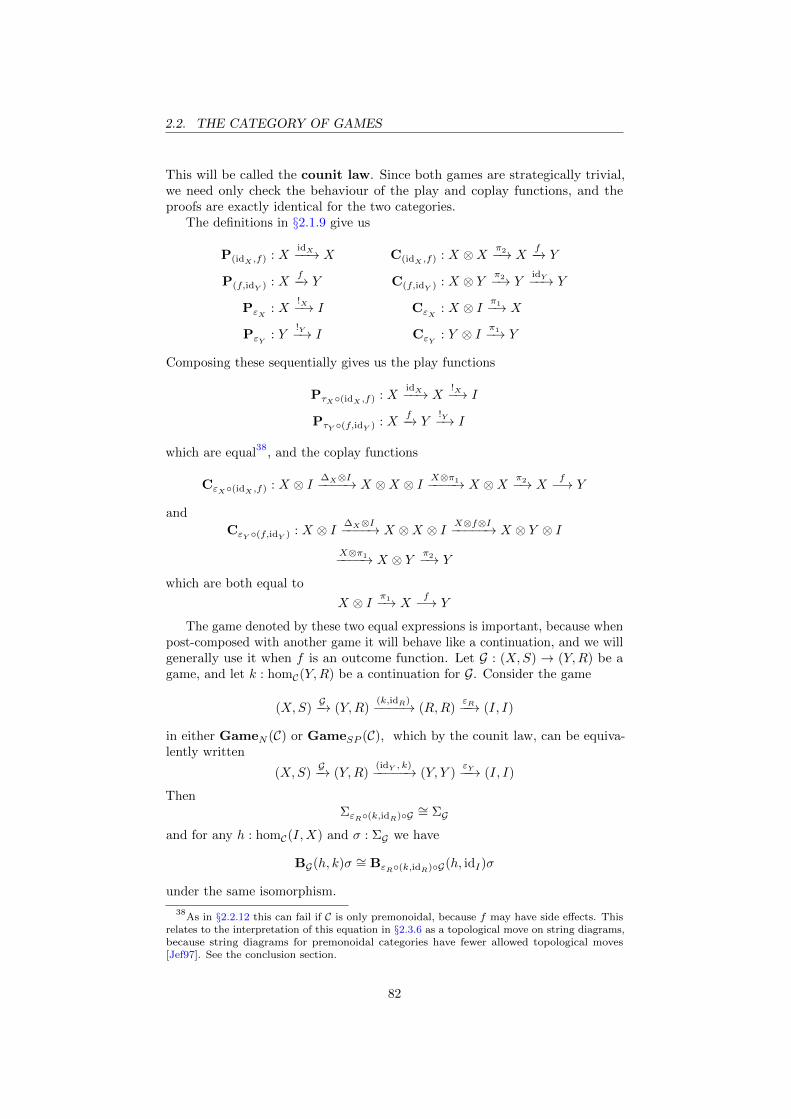
2.2. THE CATEGORY OF GAMES
This will be called the counit law. Since both games are strategically trivial,we need only check the behaviour of the play and coplay functions, and theproofs are exactly identical for the two categories.
The definitions in §2.1.9 give us
P(idX ,f) : XidX−−→ X C(idX ,f) : X ⊗X π2−→ X
f−→ Y
P(f,idY ) : Xf−→ Y C(f,idY ) : X ⊗ Y π2−→ Y
idY−−→ Y
PεX: X
!X−→ I CεX: X ⊗ I π1−→ X
PεY: Y
!Y−→ I CεY: Y ⊗ I π1−→ Y
Composing these sequentially gives us the play functions
PτX◦(idX ,f) : XidX−−→ X
!X−→ I
PτY ◦(f,idY ) : Xf−→ Y
!Y−→ I
which are equal38, and the coplay functions
CεX◦(idX ,f) : X ⊗ I ∆X⊗I−−−−→ X ⊗X ⊗ I X⊗π1−−−−→ X ⊗X π2−→ Xf−→ Y
and
CεY ◦(f,idY ) : X ⊗ I ∆X⊗I−−−−→ X ⊗X ⊗ I X⊗f⊗I−−−−−→ X ⊗ Y ⊗ IX⊗π1−−−−→ X ⊗ Y π2−→ Y
which are both equal to
X ⊗ I π1−→ Xf−→ Y
The game denoted by these two equal expressions is important, because whenpost-composed with another game it will behave like a continuation, and we willgenerally use it when f is an outcome function. Let G : (X,S) → (Y,R) be agame, and let k : homC(Y,R) be a continuation for G. Consider the game
(X,S)G−→ (Y,R)
(k,idR)−−−−→ (R,R)εR−−→ (I, I)
in either GameN (C) or GameSP (C), which by the counit law, can be equiva-lently written
(X,S)G−→ (Y,R)
(idY , k)−−−−−→ (Y, Y )εY−−→ (I, I)
ThenΣεR◦(k,idR)◦G ∼= ΣG
and for any h : homC(I,X) and σ : ΣG we have
BG(h, k)σ ∼= BεR◦(k,idR)◦G(h, idI)σ
under the same isomorphism.
38As in §2.2.12 this can fail if C is only premonoidal, because f may have side effects. This
relates to the interpretation of this equation in §2.3.6 as a topological move on string diagrams,because string diagrams for premonoidal categories have fewer allowed topological moves[Jef97]. See the conclusion section.
82

2.2. THE CATEGORY OF GAMES
To see this, the right hand side by the definition in §2.2.4 is, in GameN (C),
BεR◦N (k,idR)◦NG(h, idI)σ
= BG(h, (idI)∗◦)σ ×⋂σ′:ΣG
BεR◦(k,idR)(PGσ′ ◦ h, idI)∗
and, since εR ◦N (k, idR) is strategically trivial, this is
BG(h, (idI)∗◦)σ × {∗}
Similarly in GameSP (C),
BεR◦N (k,idR)◦NG(h, idI)σ
= BG(h, (idI)∗◦)σ ×BεR◦(k,idR)(PGσ ◦ h, idI)∗= BG(h, (idI)∗◦)σ × {∗}
The final step is to see that (idI)∗◦ = k. By definition it is
(idI)∗◦ : Y∆Y−−→ Y ⊗ Y
Y⊗PεR◦(k,idR)−−−−−−−−−−→ Y ⊗ I Y⊗idI−−−−→ Y ⊗ ICεR◦(k,idR)−−−−−−−→ R
which reduces to
Y∆Y−−→ Y ⊗ Y Y⊗!Y−−−−→ Y ⊗ I π1−→ Y
k−→ R
and hence to k.The equations
BεR◦(k,idR)◦G(h, idI)σ ∼= BG(h, k)σ ∼= BεY ◦(idY ,k)◦G(h, idI)σ
are very important because they allow us to move between ‘internal’ and ‘external’views of the continuation k. We will see this used several times in §2.3, §3.1 and§3.2, when k is an outcome or utility function.
2.2.14 Information flow in games
In §2.1 and §2.2 we have given several definitions whose intuitive justificationshave been incomplete at best. This will remain the case until chapter 3, inwhich we will demonstrate that game theory can be done inside the categoriesGameN (C) and GameSP (C). However we would also like to have a separatejustification of the ‘low level’ operations, especially for readers whose motivationscome from category theory. We have argued, for example in §2.2.4, that thedefinitions are not canonical, in the sense that there are useful variations, and so itwould be naive to expect an axiomatic definition of GameN (C) or GameSP (C),for example using universal properties.
There is, however, one known and very surprising connection to existingmathematics. The data (ΣG ,PG ,CG ,BG) specifying a game G could be dividedinto two kinds of data: the strategy profiles ΣG and best response functions BGare motivated in terms of game theory, whereas the play and coplay functionsPGσ, CGσ for a fixed strategy σ are used for information flow. These latter arestrongly reminiscent of dialectica categories.
83

2.3. STRING DIAGRAMS
The dialectica categories are categorical models of intuitionistic logic39 in-troduced in [dP91], which are based on Godel’s dialectica interpretation [AF98].The dialectica category40 D(Set) has as objects relations ϕ ⊆ X × R, whichin particular specifies a pair41 of sets (X,R). A morphism from ϕ ⊆ X × S toψ ⊆ Y ×R is a pair (f, g) where
f : X → Y
andg : X ×R→ S
such that for all x : X and r : R we have
ϕ(x, g(x, r)) =⇒ ψ(fx, r)
This has a notable similarity with f = PGσ and g = CGσ, if we take the relationsto be trivial (either both empty or both full). More importantly, the definition ofcategorical composition is essentially the same in GameN (C) and GameSP (C)as in D(C), so the definition that was claimed in §2.2.3 to not be intuitivelyjustifiable is in fact largely an instance of something already known, and theproofs in §2.2.5 and §2.2.6 partly resemble the corresponding proofs for dialecticacategories.
It should be mentioned that dialectica categories (and functional interpre-tations in proof theory) can be seen in game semantic terms, see for example[Bla97] and [Hed15a]. The relations ϕ and ψ are seen as games, in the game-semantic sense of two-player win/lose games, with (f, g) being a strategy forthe first player (proponent) and (x, r) being a strategy for the second player(opponent), in a relative game ϕ→ ψ. Then the existence of a morphism ϕ→ ψ,which logically relates to provability of the implication, amounts to the existenceof a winning strategy for the first player for ψ relative to ϕ. However, thisapparent connection between game theory and game semantics seems to be onlycoincidental (see §0.3).
Finally, morphisms between indexed containers [AGH+06] have a similarform again, and a corresponding game-semantic view appears in [Hyv14].
2.3 String diagrams
2.3.1 Discussion
String diagrams are a graphical calculus that can be used to visualise informationflow in monoidal categories. Their earliest appearance may be Penrose’s graphicaltensor notation in [Pen71], with another precursor being Girard’s proof nets for
39Dialectica models of linear logic are better known.
40This definition generalises to D(C) for C an arbitrary monoidal closed category [dP07],
and to an even more abstract setting in [Hyl02]. This suggests it may be possible to give amore axiomatic formulation of Game(C) if desired.
41There are several constructions in category theory besides dialectica categories that take
objects to be pairs, generally to obtain some form of duality. Chu spaces are already knownto be related to dialectica categories [dP07]. The Int-construction [JSV96] is better known,but has a quite different structure. That paper explicitly says that the pair (X,R) shouldbe considered as a formalisation of X ⊗R∗, as we will begin to do in §2.3.5. For remarks onduality in GameN (C), see §2.3.6 and §2.3.7.
84

2.3. STRING DIAGRAMS
linear logic [Gir87], and the mathematical foundations were formalised in [JS91].They became well known through the work of Samson Abramsky, Bob Coeckeand others on quantum information theory [Coe11], and later through the workof Bob Coecke, Mehrnoosh Sadrzadeh and others on distributional semantics inlinguistics [HSG13]. String diagrams are also being applied in other areas suchas bialgebra [McC12] and computability [Pav13].
As is the case in quantum physics and linguistics, string diagrams can be usedin game theory to visualise information flow. This visualisation is a separateissue to compositionality (although being able to compose string diagrams is acrucial requirement), and is a separate contribution of this thesis. The conceptof information flow in games will only be introduced informally and by example,starting in §2.3.9. The effect of the counit game on information flow, describedin §2.3.6, is particularly interesting, but again will only be discussed informally.
For readers unfamiliar with string diagrams, §2.3.2 and §2.3.3 introduce themin an informal way that will be sufficient for our purposes. Alternatively, [BS10]is a good introduction. A survey of the many types of string diagrams is givenin [Sel11], although the exact variant we introduce in §2.3.5 does not match anyof the usual definitions.
The purpose of string diagrams varies by discipline. In quantum informationtheory, the emphasis is generally on the ability of string diagrams to reducecomplex calculations in tensor calculus to trivial topological deformation, a pointmade forcibly in [Coe05]. In linguistics, there is more emphasis on the use ofstring diagrams as a device for visualising the logical structure of sentences,whereas the underlying categorical structure is used in a more formal way byconsidering functorial semantics.
In game theory, we will similarly emphasise string diagrams as a visualisationtool. However, more so than in linguistics, the algebraic expressions denotingeven simple games can be quite complicated, and we will make use of stringdiagrams as a tool for making definitions. A good example is in §3.2.2, where wewill define a particular game by its (simple) string diagram, and the subsequentwork to compute the denotation of the string diagram is quite involved. However,this work could quite easily be automated, as described in the conclusion.
It should be noted that this thesis does not contain a theorem that charac-terises exactly the topological moves which are allowed on string diagrams; manyare proved to be valid, and some are known to be invalid, but it has not beenproved that this exhausts all possible moves. In the absence of such a theorem,we cannot strictly speak about ‘the game denoted by a string diagram’, becauseit cannot be ruled out that a topologically equivalent string diagram denotesa different game. Therefore every string diagram should, for the time being,be accompanied by an algebraic term (with operators ◦N and ⊗) showing theintended reading.
2.3.2 String diagrams for monoidal categories
The basic components of string diagrams are strings and beads. A simplestring diagram has the form
X Yf
85

2.3. STRING DIAGRAMS
This string diagram denotes a morphism f : X → Y in some monoidal category.The strings in the diagram are labelled by objects of the category, and the beadsby morphisms.
The composition of the category is denoted by end-to-end composition ofstring diagrams. If we have morphisms f : X → Y and g : Y → Z, thecomposition g ◦ f : X → Z is denoted by
X Zf gY
Notice that the associativity of composition is trivialised, because there is onlyone way to graphically compose three morphisms. This is the simplest exampleof a powerful fact about string diagrams, that coherence conditions in a categoryare reduced to graphical identity or topological deformation.
The other way of composing morphisms, namely the tensor product, isdenoted by side-by-side composition. If we have morphisms f1 : X1 → Y1 andf2 : X2 → Y2, the tensor product f1 ⊗ f2 : X1 ⊗X2 → Y1 ⊗ Y2 is denoted by
X1 Y1
X2 Y2
f1
f2
Again, notice that the associator of the tensor product is reduced to graphicalidentity. According to these rules, the string diagram
X1 Z1
X2 Z2
f1 g1
f2 g2
Y1
Y2
could denote either (g1◦f1)⊗(g2◦f2) or (g1⊗g2)◦(f1⊗f2) : X1⊗X2 → Z1⊗Z2,but these are equal42.
A morphism f : X1 ⊗ X2 → Y1 ⊗ Y2 ⊗ Y3 is denoted by a bead with twostrings entering on the left and three exiting on the right:
X1
X2
f
Y1
Y2
Y3
42This is the axiom that ⊗ is a bifunctor.
86

2.3. STRING DIAGRAMS
The unit object of the tensor product is denoted by empty space. For example,if we have morphisms f : I → X and g : X → I, the composition g ◦ f : I → Iis denoted by
f gX
The identity morphism on an object X is denoted by simply a string labelledwith X. The coherence laws for the identity morphisms and unit object areagain reduced to topological deformations.
2.3.3 Compact closed categories
An important structure that a monoidal category C can carry, which has aparticularly elegant interpretation in string diagrams, is that of a compact closedcategory. In a compact closed category we have a duality, which is43 a monoidalfunctor −∗ : C → Cop. The prototypical example of a compact closed categoryis the category of finite-dimensional vector spaces and linear maps over a fixedfield, with duality given by duality of vector spaces; another well known exampleis the category of sets and relations, with duality being the identity on sets, andgiving inverse relations.
Whereas an object X is denoted by an X-labelled string running from leftto right, the dual object X∗ is denoted by an X-labelled string running fromright to left. Then, given a morphism f : X → Y denoted by
X Yf
we will denote the dual morphism f∗ : Y ∗ → X∗ by its rotation:
Y Xf
The tensor product is still denoted by side-by-side composition, and so forexample a morphism f : X ⊗ S∗ → Y ⊗R∗ in a compact closed category wouldbe denoted by
X
S
f
Y
R
We additionally have unit morphisms ηX : I → X ⊗X∗ denoted by a cap44
X
X
43This is not intended to be a rigorous introduction to compact closure, but rather to develop
intuition that we can use starting in §2.3.5.44
The ‘cap’ and ‘cup’ terminology makes more sense if we draw time running from top tobottom rather than right to left.
87

2.3. STRING DIAGRAMS
and counits εX : X ⊗X∗ → I denoted by a cup
X
X
The axioms of a compact closed category specify precisely that the units andcounits behave in graphically intuitive ways. For example, a bent string can bestraightened (this is called the ‘yanking equation’),
X X = X X
and a bead can be slid around a cap or cup:
X
Y
f
=
X
Y f
Combining these, we can topologically deform a string diagram in arbitrary ways,for example we can equally denote a morphism f : X → Y by the string diagram
X Yf
2.3.4 Boxing and compositionality
A simple but very important observation is that string diagrams are inherentlyfully compositional. Given an arbitrary string diagram, we could make itdefinitionally equal to a single bead, preserving only the strings entering andleaving the diagram. Such strings will be called open ports. To give an example,suppose we have morphisms f : X → Y and g : Y → Z, and we define a newmorphism
(Y ⊗ g) ◦∆Y ◦ f : X → Y ⊗ Z
which is denoted by the string diagram
88

2.3. STRING DIAGRAMS
X f
g
Y
Z
This string diagram has an X-labelled open port entering to the left, and Y -and Z-labelled open ports leaving to the right. If we define h : X → Y ⊗ Z tobe this morphism, then we can replace this string diagram with
X h
Y
Z
This amounts to forgetting the definition of h and remembering only its type,that is to say, the types, order and variance of its open ports.
We can imagine that if we zoom in to the h-labelled bead in this stringdiagram, we will come to the previous string diagram, with the open portsbeing physically the same as the strings attached to the h-labelled bead (see theconclusion section).
Conversely, the act of obtaining the lower string diagram from the upperamounts to drawing a box around the entire diagram, so that the points at whichthe open strings intersect the box become exactly the points at which the stringsenter and leave the h-labelled bead. We will refer to this as boxing the stringdiagram, and it is the graphical analogue of making a definitional equality.
Boxing is the aspect of compositionality that can be used to work in a scalableway. In a more serious example, the morphism h could be a very complicatedprocess, which we can then use and re-use without worrying (or even knowing)how it is defined. In software engineering, the boxed morphism would variouslybe known as a ‘type’, a ‘signature’ or an ‘interface’.
2.3.5 The geometry of games
The idea behind string diagrams in game theory is that although GameN (C)does not have as much structure as the categories usually considered with stringdiagrams, we will abuse notation as though we had this structure. A gameG : (X,S)→ (Y,R) will be denoted by the string diagram
X
S
G
Y
R
That is, we are pretending that GameN (C) has a duality −∗, and that G is amorphism G : X ⊗ S∗ → Y ⊗R∗.
This is a reasonable thing to do. If we define an operation on objects by(X,R)∗ = (R,X), we find that this operation can be extended in a compatibleway to some morphisms, but not all. Thus we can consider −∗ to be a partialfunctor, which is total on objects (that is, a ‘functor’ whose underlying function
89

2.3. STRING DIAGRAMS
on morphisms is weakened to only a partial function; alternatively it is a functordefined on a suitable wide subcategory). Since we have a symmetric monoidalembedding C ↪→ GameN (C) (§2.2.12), we can write X and R for (X, I) and(R, I). Thus R∗ = (I,R), and so X⊗R∗ = (X, I)⊗(I,R) = (X⊗I, I⊗R) which,treating natural isomorphism as though it is identity, gives X ⊗R∗ = (X,R).
We will extend this notation in several intuitive ways. For example, if wehave a game
G : (X1 ⊗X2, S1 ⊗ S2)→ (Y1 ⊗ Y2, R1 ⊗R2)
we may write it as
G : X1 ⊗ S∗1 ⊗X2 ⊗ S
∗2 → Y1 ⊗R
∗1 ⊗ Y2 ⊗R
∗2
(among many other possibilities, one for each permutation), and the stringdiagram as
X1
X2
Y1
Y2
R1
R2
S1
S2
G
In general, we will be unconcerned but consistent with the order of the types insuch situations.
Of course this comes at a cost: not all topological operations on our stringdiagrams preserve meaning, or even well-formedness. This is something wewill need to take extra care about. For example, in a compact closed categorythere is no real distinction between ‘past’ and ‘future’, but in GameN (C) theyare distinct: a game G : X → Y cannot be turned into G : I → X∗ ⊗ Y . Anexplanation for this is given in §2.3.12.
We will omit some strings when some of the types involved are the monoidalunit. For example, if we have a decision D : (X, I)→ (Y,R) then we will writeD : X → Y ⊗R∗, and the string diagram denoting it is
X D
Y
R
A closed game could be denoted simply by a bead with no strings attached.
2.3.6 Partial duality
A computation (f, g) : (X,S)→ (Y,R) will be denoted by the string diagram
90

2.3. STRING DIAGRAMS
X Y
RS
f
g
That is, we are pretending that (f, g) = f ⊗ g∗, where g∗ : S∗ → R∗ is thedual of g. This is another case of treating −∗ as a partial functor, this timedefined on morphisms of C. From this point onwards we will no longer treatcomputations formally as pairs (f, g), but as individual games f and g∗ which wetensor together when necessary. This is an extension of the fact that computationis a monoidal embedding (§2.2.12). For example, if g : R→ S then we can writeg∗ = (idI , g) : S∗ → R∗ and use the string diagram
RS g
since idI is denoted by empty space.The counit game εX : (X,X)→ (I, I) can now be written εX : X ⊗X∗ → I,
and will be denoted by a cup
X
X
The counit lawεY ◦ (f, idY ) = εX ◦ (idX , f)
which we proved in §2.2.13 now appears as a coherence law
X
Y
f
=
X
Y f
telling us that we can slide a computation around the counit like a bead. Thistakes the same form as the coherence law for the counit of a compact closedcategory (see §2.3.3), but applies only45 to computations.
The partiality of the duality means that, unlike in a compact closed category,we cannot rotate beads. For example, in a compact closed category we have avalid equation
X X = X X
45It is unknown whether Game(C) contains any dualisable morphisms besides the computa-
tions.
91

2.3. STRING DIAGRAMS
but we cannot do so here because the cap does not denote a morphism ofGameN (C), so the left hand side is not a well formed string diagram.
2.3.7 Covariance, contravariance and symmetries
This kind of duality has one strange consequence, concerning how covariant andcontravariant (or forward and backward) strings interact. If we have two stringspointing in the same direction which cross, such as
X
Y
Y
X
then the denoted morphism is a symmetry σX,Y : X ⊗ Y → Y ⊗X, or moreformally, the computation
(σX,Y , idI) : (X ⊗ Y, I)→ (Y ⊗X, I)
Similarly, in the contravariant direction, the string diagram
Y
X
X
Y
denotes σ∗X,Y : Y ∗ ⊗X∗ → X∗ ⊗ Y ∗, or again more formally,
(idI , σX,Y ) : (I, Y ⊗X)→ (I,X ⊗ Y )
However, now consider the string diagram
X
Y
Y
X
The object on the left is X ⊗ Y ∗, which formally denotes (X,Y ). The object onthe right is Y ∗ ⊗X, which again formally denotes (X,Y ). Thus, the denotationσX,Y ∗ of this string diagram is an identity, not a symmetry.
More generally, if we have a string diagram which consists only of crossingsof covariant and contravariant strings, the denoted game is an identity. We willsee this in practice in the coming sections, for example in §2.3.9.
92

2.3. STRING DIAGRAMS
Another example of the same idea is drawing a counit with the oppositeorientation than in §2.3.6. This is justified by the topological deformation
X
X
=
X
X
where the right hand side is the composition εX ◦ σX∗,X , because the symmetryσX∗,X is trivial.
2.3.8 Copying and deleting information
The underlying categories C introduced in §2.1.2 are not compact closed ingeneral, but they do have one piece of additional structure assumed, namelythat every object is a cocommutative coalgebra in a canonical way. This meansthat we have canonical morphisms
!X : X → I
and∆X : X → X ⊗X
for each object X. These morphisms can be lifted into GameN (C) eithercovariantly, or contravariantly as
!∗X : I → X∗
and∆∗X : X∗ ⊗X∗ → X∗
Thus, the covariant objects46 of GameN (C) are cocommutative coalgebras, andcontravariant objects are commutative algebras.
As is usual with string diagrams, we will denote the algebraic and coalgebraicoperators by small filled circles. That is, the coalgebraic operators on a covariantobject are denoted by
X X
X
X
and the algebraic operators on a contravariant object by their rotations
X
X
X
X
46A ‘covariant object’ is an object of the form (X, I), and a ‘contravariant object’ is of the
form (I,X). A general object is the tensor product of a covariant part and a contravariantpart, and carries neither an algebra or a coalgebra structure.
93

2.3. STRING DIAGRAMS
These operators are not as ubiquitous in game theory as they are, for example,in quantum information theory47, but nearly every game will involve copyinginformation at some point in its definition, for example if both a player and autility function need to be aware of the same value.
2.3.9 A bimatrix game
We have now, finally, built up enough theory to give some recognisable, textbookexamples of games. We will begin with a bimatrix game, with mixed strategyNash equilibrium as the solution concept.
Bimatrix games are two player classical games with mixed strategies, intro-duced in §1.2.6. Thus we have two players, who simultaneously make choices fromsets X, Y . For simplicity, we will assume that these are finite. We additionallyhave utility functions q1, q2 : X × Y → R that give the utility for each player oneach play.
The best response function for such a game is
B(σ1, σ2) =
(σ′1, σ′2) : DX ×DY
∣∣∣∣∣∣E[q1(σ′1, σ2)] ≥ E[q1(x′, σ2)],E[q2(σ1, σ
′2)] ≥ E[q2(σ1, y
′)]for all x′ : X and y′ : Y
and a mixed strategy Nash equilibrium is a fixpoint of this B.
A prototypical example of a bimatrix game is matching pennies. In thisexample, we have X = Y = {H,T}, with
q1(x, y) =
{1 if x = y
0 if x 6= y
and q2(x, y) = 1 − q1(x, y). The unique mixed strategy Nash equilibrium ofthis game is the strategy profile in which both players choose either H or Twith probability 1
2 , with the expected utility for both players being 12 . Other
well known examples of bimatrix games include the prisoner’s dilemma andthe chicken game, and can be found in myriad books and lecture notes onintroductory game theory.
In order to model a bimatrix game, let G be the game in GameN (SRel)denoted by the string diagram
D1
D2
q1
q2
X
Y
R
R
47See for example the ZX-calculus [CD11].
94
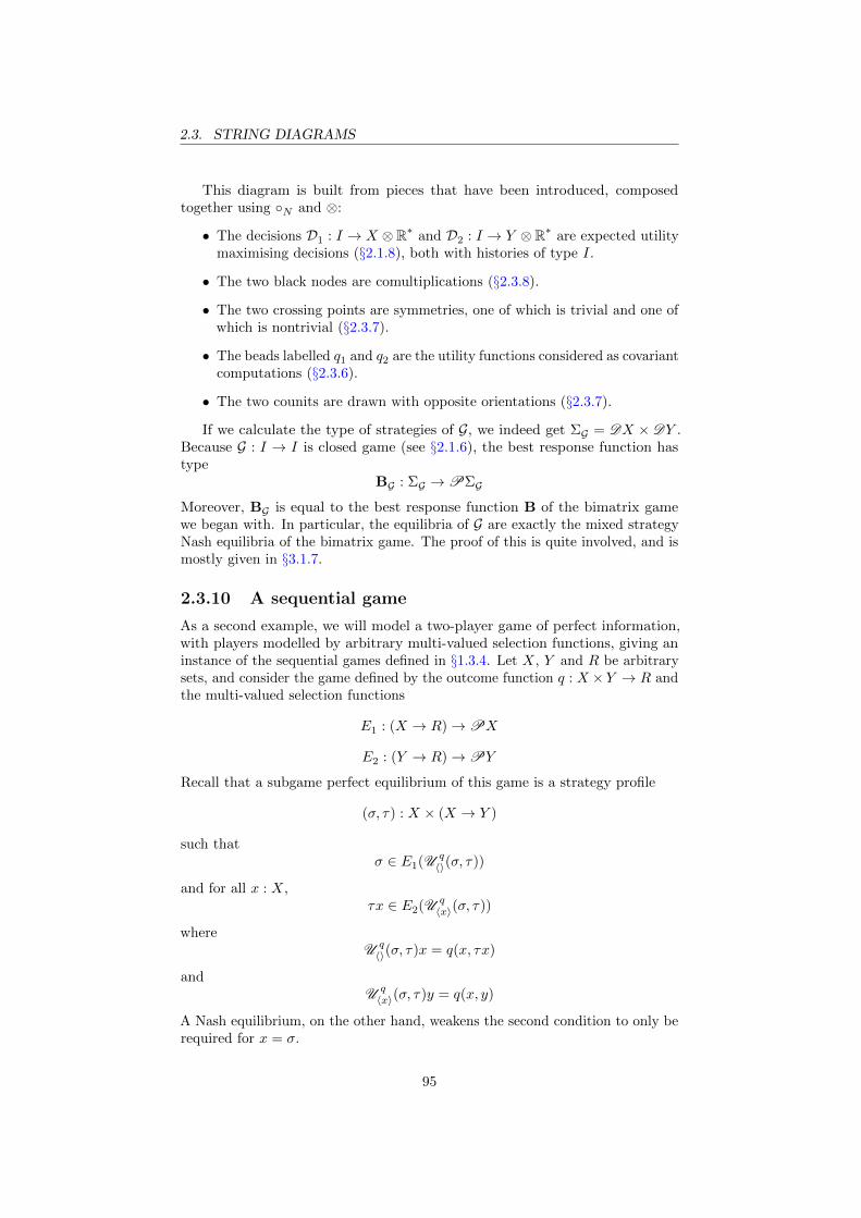
2.3. STRING DIAGRAMS
This diagram is built from pieces that have been introduced, composedtogether using ◦N and ⊗:
• The decisions D1 : I → X ⊗ R∗ and D2 : I → Y ⊗ R∗ are expected utilitymaximising decisions (§2.1.8), both with histories of type I.
• The two black nodes are comultiplications (§2.3.8).
• The two crossing points are symmetries, one of which is trivial and one ofwhich is nontrivial (§2.3.7).
• The beads labelled q1 and q2 are the utility functions considered as covariantcomputations (§2.3.6).
• The two counits are drawn with opposite orientations (§2.3.7).
If we calculate the type of strategies of G, we indeed get ΣG = DX × DY .Because G : I → I is closed game (see §2.1.6), the best response function hastype
BG : ΣG →PΣG
Moreover, BG is equal to the best response function B of the bimatrix gamewe began with. In particular, the equilibria of G are exactly the mixed strategyNash equilibria of the bimatrix game. The proof of this is quite involved, and ismostly given in §3.1.7.
2.3.10 A sequential game
As a second example, we will model a two-player game of perfect information,with players modelled by arbitrary multi-valued selection functions, giving aninstance of the sequential games defined in §1.3.4. Let X, Y and R be arbitrarysets, and consider the game defined by the outcome function q : X ×Y → R andthe multi-valued selection functions
E1 : (X → R)→PX
E2 : (Y → R)→PY
Recall that a subgame perfect equilibrium of this game is a strategy profile
(σ, τ) : X × (X → Y )
such thatσ ∈ E1(U q
〈〉(σ, τ))
and for all x : X,τx ∈ E2(U q
〈x〉(σ, τ))
whereU q〈〉(σ, τ)x = q(x, τx)
andU q〈x〉(σ, τ)y = q(x, y)
A Nash equilibrium, on the other hand, weakens the second condition to only berequired for x = σ.
95

2.3. STRING DIAGRAMS
Let D1 : I → X ⊗R∗ be the decision in Game(Set) defined by the responsefunction
RD1(∗, k) = E1k
and let D2 : X → Y ⊗R∗ be the decision defined by
RD2(x, k) = {τ ′ : X → Y | τ ′x ∈ E2k}
These are instances of the construction in §2.1.7 of a decision from a multi-valuedselection function.
Let G : I → I be the closed game in GameN (Set) denoted by the stringdiagram
D1 D2
q
X
X
X
Y R
R
R
or the algebraic expression
G = τR ◦N (q ⊗∆∗R) ◦N (X ⊗D2 ⊗R∗) ◦N (∆X ⊗R
∗) ◦N D1
The set of strategy profiles for this game is ΣG = X×(X → Y ), and the fixpointsof BG : ΣG →PΣG are precisely the Nash equilibria.
On the other hand, if we use SP -composition rather than N -compositionthen BG is precisely the best response function in §1.3.5, whose fixpoints are thesubgame perfect equilibria. However, because GameSP (Set) is only premonoidalthe string diagram language is not well-defined, and we can only use the algebraicexpression.
This example can also be extended in a graphically intuitive way to gamesof imperfect information, in which the second player can only observe somefunction of the first player’s choice. The construction will be sketched in §3.2.7,although full proofs will not be given.
2.3.11 Coordination and differentiation games
As our final introductory example, we will return to the coordinating anddifferentiating behaviour of §1.2.9. As in the voting game introduced in §1.2.7,we will let X be finite and consider the outcomes to also be R = X. We willconsider a pair of decisions
Dfix,Dnonfix : I → X ⊗X∗
96

2.3. STRING DIAGRAMS
in GameN (Set), defined by the response functions given exactly by the multi-valued selection functions Efix and Enonfix, so
BDfix(∗, k)σ = Efixk
BDnonfix(∗, k)σ = Enonfixk
Consider the string diagram
D1
D2
X
X
where D1 and D2 are chosen from Dfix and Dnonfix. One way to write thisalgebraically is
G = (εX ⊗ εX) ◦ (sX,X ⊗X∗ ⊗X∗) ◦ (D1 ⊗D2) : I → I
The type of strategy profiles is ΣG = X ×X. The best response functionBG : X ×X →P(X ×X) is given by
BG(σ, τ) = BD1(∗, k1)σ ×BD2
(∗, k2)τ
where k1x = τ and k2x = σ are constant functions. Since σ′ ∈ BDfix(∗, k1)σ iff
σ′ = τ , and τ ′ ∈ BDfix(∗, k2)τ iff τ ′ = σ, if we take D1 = D2 = Dfix then (σ, τ)
is an equilibrium of G iff σ = τ . Similarly, if we take D1 = D2 = Dnonfix then(σ, τ) is an equilibrium of G iff σ 6= τ . Thus we again obtain coordinating anddifferentiating behaviour.
If we take D1 = Dfix and D2 = Dnonfix then G has no equilibria, because for(σ, τ) to be an equilibrium we must have both σ = τ and σ 6= τ . It would beinteresting to consider variants of Dfix and Dnonfix in GameN (SRel), becausethis game48 should intuitively have a mixed strategy Nash equilibrium, but thisis not free because we cannot take the mixed extension of a selection function(see §1.2.6).
This example demonstrates that open games can model non-classical prefer-ences described by selection functions. It is interesting because the game has nooutcome function in a very literal sense, but instead the string diagram visualisesthe information flow where each player directly reasons about the move of theother. However this issue is orthogonal to compositionality, and we will notdiscuss it further.
48This game is called the penalty game because it models a penalty shootout. The fixpoint
player is the goalkeeper who would like to coordinate, and the non-fixpoint player is the penaltytaker who would like to differentiate.
97

2.3. STRING DIAGRAMS
2.3.12 Designing for compositionality
We now return to theoretical considerations, having gained some intuition aboutthe possible examples. The fact that the counit εX is not dualisable has someinteresting consequences for information flow in GameN (C). A game of typeG : X ⊗S∗ → Y ⊗R∗ can be thought of as accepting a value of type X from thepast, and a value of type R from the future (see §2.1.4). If we have a value oftype R in the past (for example, because an agent’s utility is determined entirelyby events in the past) then we can use the counit to bend the string around, asin
X Y
R
S
G
To put it another way: a value known in the past will still be known in the future.On the other hand, if we only have a value of type X in the future, we cannot
use it (unlike in a compact closed category) because an agent cannot directlyobserve the future, but only reason about it (which is the purpose of R). This‘causality’ point of view suggests a heuristic explanation of why GameN (C) hasthe structure that it does, namely that −∗ behaves in some ways like a duality,but is not a functor. Indeed, if GameN (C) were compact closed it would bestraightforward to construct a paradoxical situation analogous to the grandfatherparadox, in which a strategy negates the value chosen by itself. Categories withmore structure typically get around this problem using a ‘failure’ state such asthe zero vector, the empty relation or the nonterminating computation.
This will have a major impact on design for compositionality, which maybecome an important research topic in applied compositional game theory. In§3.1 and §3.2 we will show that certain known, simple classes of classical gamescan be faithfully represented as closed games. The purpose of this, as describedin §0.5, is to show formally that compositional game theory is indeed gametheory. However, a practical use of compositional game theory will likely lookquite different.
In §2.3.9 we represented a bimatrix game as a closed game G : I → I. Sincethe game is closed, there is no nontrivial way in which it can interact with itsenvironment, and consequently there is no nontrivial way to compose it withother games. This is unsurprising, because the point was to produce a faithfulmodel of a classical bimatrix game, and classical bimatrix games do not interactwith their environment, that is to say, they cannot be composed.
The question of how a bimatrix game should be represented in order toallow compositionality is a nontrivial modelling problem: we want to modelthe bimatrix game as an open game so that it could be reused in later, morecomplicated problems. The simpler half of this problem is what to take for Y andS, the types of values flowing from the game to its environment: a reasonablechoice is Y = X ′ ⊗ Y ′, where X ′ and Y ′ are the types of choices made by the
98

2.3. STRING DIAGRAMS
two players49, and S = I, because there is no useful sense in which the bimatrixgame can generate coutility.
The type X, given suitable features50 of the underlying category C, could varyover all nonempty finite sets, with the game being parametrically polymorphicin X. The decisions, as defined in §2.1.8, do indeed seem to be parametricallypolymorphic in X. The non-compositional example in §2.3.9 is recovered bysetting X = I.
The difficult case is R. The problem is to determine how the utility of twoconcrete players should be affected by unknown events in the future. The simplestway to deal with this is to take R = R⊗R and use the well-understood ubiquityof real-valued utility as a ‘universal representation’, receiving an additional utilityfrom the future that is simply added to the utility for each player from the gameitself. The string diagram corresponding to this description is
D
D
q1
q2
+
+
R
R
X
Y
R
R
R
R
One notable drawback of this is that the preferences of the players, whichdetermine the appropriate utilities, become distributed throughout the stringdiagram rather than being localised. A possible alternative approach would beto have a game that is parametric in both a type R and in a rational preferencerelation on R. In any particular instantiation, the type and preference relationcould be chosen depending on the modelling problem at hand.
49In §2.3.9 X
′and Y
′are called X and Y , and should not be confused with the ‘default’
use of X and Y in §2.1.4 and elsewhere.50
The motivating example is the type system of Haskell (see §0.2). Writing in a parametricallypolymorphic way is second nature to a functional programmer.
99

Chapter 3
Game theory via opengames
3.1 Normal form games
3.1.1 Discussion
In chapter 2 of this thesis we have built up an abstract theory, and this will becontinued in §3.3 when we study solvability of games. The central argument beinglaid out (see the conclusion for a self-contained version) is that this approachto game theory is better than classical approaches, at least insofar as it is morescalable. However a vital piece of the argument is missing: other than thelanguage used in the informal explanations, and the examples without proof atthe end of §2.3, we have not demonstrated that open games have any connectionat all with game theory.
The purpose of this chapter is to show that our theory does agree withclassical game theory in certain situations, specifically normal form games withpure and mixed Nash equilibria, and certain extensive form games with subgameperfect equilibria. Given a classical game theoretic situation, we should be able todraw a string diagram that looks like the information flow in the target situation,and which moreover denotes the same game. In order to discuss sameness ofgames, without even having a common framework, we will use the approachdiscussed in §1.2.4: two games will be considered the same if they have thesame sets of strategies Σ, and the same best response functions B : Σ→PΣ.As we saw in §2.1.6, an abstract scalar in GameN (Set) or GameN (SRel) isdefined precisely by Σ and B of this type. Therefore our aim is, given someexisting notion of game, to construct an abstract scalar whose strategies andbest responses are the same.
Game theory is a large subject, with entire areas devoted to various extensionsand special cases of the basic definitions. For this reason there cannot be (andnor should there be) a single theorem that subsumes classical game theory intoour new framework. For now, we are going to focus on some simple and commonspecial cases. In this section, we begin with normal form finite games and purestrategies, as introduced in §1.2, and we will prove that every such game canbe translated into a string diagram, whose strategies and Nash equilibria are
100

3.1. NORMAL FORM GAMES
the same. For additional simplicity we will work only with classical games (see§1.2.5), in order that this section can be understood only in terms of classicalgame theory, such as is introduced in [LBS08], without requiring knowledge ofselection functions. The proofs in this section and §3.2 generalise immediately toarbitrary selection functions, using the translation from multi-valued selectionfunctions to decisions in §2.1.7.
Beginning with §3.1.6, we will also show the same result for normal formgames and mixed strategies, which is the setting in which Nash proved his famousexistence theorem [Nas50].
3.1.2 Tensor products of decisions
Consider a finite normal form classical game, in the sense of §1.2.5. We haveN ≥ 1 players, where the ith player makes a choice from the finite set Xi, andreceives a real-valued utility, which she aims to maximise. Since the choices innormal form games take place simultaneously, no player observes any history.Since we are intending to model pure strategies, which involve no side effects,we will work in the category GameN (Set). The choice of the ith player willtherefore be modelled by the utility-maximising decision
Di : I → Xi ⊗ R∗
which is given as the first example in §2.1.8. For completeness, this is defined bythe data
• ΣDi = Xi
• PDiσ∗ = σ
• CDiσ(x, u) = ∗
• BDikσ = {σ′ : Xi | kσ′ ≥ kx′ for all x′ : Xi}
The purpose of this section is to study the tensor product of finitely many suchdecisions.
We will work by induction on N , the number of players. Define a game
GN : I →N⊗i=1
Xi ⊗ (R∗)⊗N
where (R∗)⊗N denotes the N -fold tensor R∗ ⊗ · · · ⊗ R∗, by
GN =
N⊗i=1
Di
More formally, we recursively define G1 = D1, and GN+1 = GN ⊗DN+1.Our task is to find a closed form description of GN . It is simple to see that
the set of strategy profiles is a cartesian product
ΣGN =
N∏i=1
Xi
101
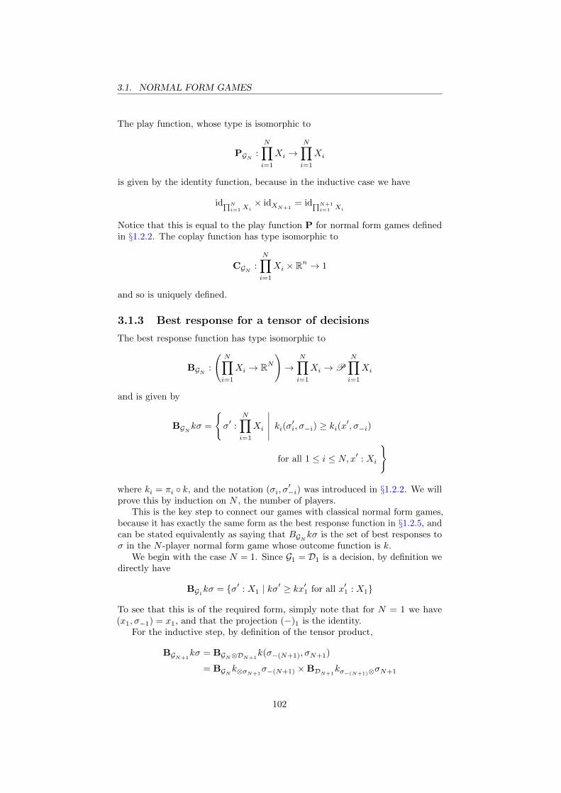
3.1. NORMAL FORM GAMES
The play function, whose type is isomorphic to
PGN :
N∏i=1
Xi →N∏i=1
Xi
is given by the identity function, because in the inductive case we have
id∏Ni=1Xi
× idXN+1= id∏N+1
i=1 Xi
Notice that this is equal to the play function P for normal form games definedin §1.2.2. The coplay function has type isomorphic to
CGN :
N∏i=1
Xi × Rn → 1
and so is uniquely defined.
3.1.3 Best response for a tensor of decisions
The best response function has type isomorphic to
BGN :
(N∏i=1
Xi → RN)→
N∏i=1
Xi →PN∏i=1
Xi
and is given by
BGNkσ =
{σ′ :
N∏i=1
Xi
∣∣∣∣∣ ki(σ′i, σ−i) ≥ ki(x′, σ−i)for all 1 ≤ i ≤ N, x′ : Xi
}
where ki = πi ◦ k, and the notation (σi, σ′−i) was introduced in §1.2.2. We will
prove this by induction on N , the number of players.This is the key step to connect our games with classical normal form games,
because it has exactly the same form as the best response function in §1.2.5, andcan be stated equivalently as saying that BGNkσ is the set of best responses toσ in the N -player normal form game whose outcome function is k.
We begin with the case N = 1. Since G1 = D1 is a decision, by definition wedirectly have
BG1kσ = {σ′ : X1 | kσ′ ≥ kx′1 for all x′1 : X1}
To see that this is of the required form, simply note that for N = 1 we have(x1, σ−1) = x1, and that the projection (−)1 is the identity.
For the inductive step, by definition of the tensor product,
BGN+1kσ = BGN⊗DN+1
k(σ−(N+1), σN+1)
= BGNk⊗σN+1σ−(N+1) ×BDN+1
kσ−(N+1)⊗σN+1
102

3.1. NORMAL FORM GAMES
We introduce here the less cluttered notation k⊗σN+1and kσ−(N+1)⊗ as shorthand
for k⊗σN+1(∗) and kσ−(N+1)(∗)⊗ (see §2.2.7), because all histories are trivial fordecisions in normal form games.
Before we proceed further, we must explicitly calculate k⊗σN and kσ−(N+1)⊗.The original continuation is
k :
N+1∏i=1
Xi → RN+1
which we will write in the isomorphic form
k :
N∏i=1
Xi ×XN+1 → RN × R
The left continuation k⊗σN+1:∏Ni=1Xi → RN is, by the definition in §2.2.7,
given by
N∏i=1
Xi
∼=−→N∏i=1
Xi × 1
∏Ni=1Xi×PDN+1
σN+1
−−−−−−−−−−−−−−−→N∏i=1
Xi ×XN+1
k−→ RN × Rπ−(N+1)−−−−−→ RN
Since DN+1 is a decision in GameN (Set) its play function is
PDN+1σN+1∗ = σN+1
so this is simplyk⊗σN+1
σ′ = k−(N+1)(σ′, σN+1)
Similarly the right continuation kσ−(N+1)⊗ : XN+1 → R by definition is
XN+1
∼=−→ 1×XN+1
PGNσ−(N+1)∗×XN+1−−−−−−−−−−−−−−→
N∏i=1
Xi ×XN+1
k−→ RN × RπN+1−−−→ R
Since we have already checked in the previous section that
PGNσ−(N+1)∗ = σ−(N+1)
this is explicitlykσ−(N+1)⊗σ
′ = kN+1(σ−(N+1), σ′)
3.1.4 Best response for a tensor of decisions, continued
We can now expand
BGN+1kσ = BGNk⊗σN+1
σ−(N+1) ×BDN+1kσ−(N+1)⊗σN+1
The first term BGNk⊗σN+1σ−(N+1), by the inductive hypothesis, is the set of
σ′ :∏Ni=1Xi such that for all 1 ≤ i ≤ N and x′i : Xi,
(k⊗σN+1)i(σ
′i, (σ−(N+1))−i) ≥ (k⊗σN+1
)i(x′i, (σ−(N+1))−i)
103
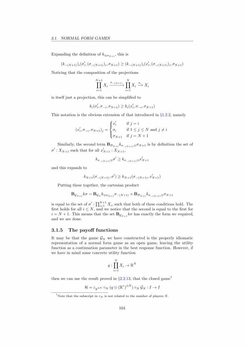
3.1. NORMAL FORM GAMES
Expanding the definition of k⊗σN+1, this is
(k−(N+1))i(σ′i, (σ−(N+1))i, σN+1) ≥ (k−(N+1))i(x
′i, (σ−(N+1))i, σN+1)
Noticing that the composition of the projections
N+1∏i=1
Xi
π−(N+1)−−−−−→N∏i=1
Xiπi−→ Xi
is itself just a projection, this can be simplified to
ki(σ′i, σ−i, σN+1) ≥ ki(x
′i, σ−i, σN+1)
This notation is the obvious extension of that introduced in §1.2.2, namely
(x′i, σ−i, σN+1)j =
x′i if j = i
σi if 1 ≤ j ≤ N and j 6= i
σN+1 if j = N + 1
Similarly, the second term BDN+1kσ−(N+1)⊗σN+1 is by definition the set of
σ′ : XN+1 such that for all x′N+1 : XN+1,
kσ−(N+1)⊗σ′ ≥ kσ−(N+1)⊗x
′N+1
and this expands to
kN+1(σ−(N+1), σ′) ≥ kN+1(σ−(N+1), x
′N+1)
Putting these together, the cartesian product
BGN+1kσ = BGNk⊗σN+1
σ−(N+1) ×BDN+1kσ−(N+1)⊗σN+1
is equal to the set of σ′ :∏N+1i=1 Xi, such that both of these conditions hold. The
first holds for all i ≤ N , and we notice that the second is equal to the first fori = N + 1. This means that the set BGN+1
kσ has exactly the form we required,and we are done.
3.1.5 The payoff functions
It may be that the game GN we have constructed is the properly idiomaticrepresentation of a normal form game as an open game, leaving the utilityfunction as a continuation parameter in the best response function. However, ifwe have in mind some concrete utility function
q :
N∏i=1
Xi → RN
then we can use the result proved in §2.2.13, that the closed game1
H = εR⊗N ◦N (q ⊗ (R∗)⊗N ) ◦N GN : I → I
1Note that the subscript in ◦N is not related to the number of players N .
104

3.1. NORMAL FORM GAMES
has the property thatBGN qσ = BH∗σ
Therefore ΣH = ΣGN and BH : ΣGN →PΣGN specify the same strategies andbest responses for H as for the classical normal form game we began with. Asdiscussed in §3.1.1, this is precisely the aim we began with.
Because computations are a monoidal embedding, we can go further anddecompose q, so that the information flow inside q is visible in the string diagram.Typically, q is constructed by beginning with a utility function
qi :
N∏i=1
Xi → R
for each player i. The tensor product of these, considered as covariant computa-tions, is
N⊗i=1
qi :
N⊗i=1
N⊗j=1
Xj → R⊗N
Since each of the N utility functions requires access to all N choices, we needto copy each choice N times and then braid them into the right order. This isimplemented by a copy followed by symmetries. For example, when N = 3 weuse
X1
X2
X3
q1
q2
q3
R
R
R
In general2, the copying is implemented by a covariant computation
N⊗i=1
Xi →N⊗i=1
N⊗j=1
Xj
2Doing this in a somewhat compositional way is possible, but tedious. It is unavoidable to
fix the number N , and eventually we will come up against the fact that outcome functionsare fundamentally not compositional, because they refer to the totality of all players. Findingways to avoid this may become a significant research problem in applied compositional gametheory.
105

3.1. NORMAL FORM GAMES
whose play function is
P(x1, . . . , xN ) = (x1, . . . , xN , . . . , x1, . . . , xN )
Of course, particular features such as common subexpressions can be used tosimplify such a string diagram in many examples.
The example game in §2.3.9 has this form, but uses mixed strategies, whichwe will now develop. In the remainder of this section, and in §3.2, we willwork with the open form of a game, leaving the outcome function implicit as acontinuation parameter in the best response function.
3.1.6 Stochastic decisions
The result that normal form games can be faithfully represented as open gamesalso holds if we change our solution concept from pure to mixed strategy Nashequilibrium. Mixed strategy Nash equilibria of classical games were introducedin §1.2.6. Following the example in §2.3.9 we now describe the general case,making use of the probability distribution monad D introduced in §2.1.3.
We will now work in the category GameN (SRel), where SRel is the Kleislicategory of D . Following §3.1.2, we have a sequence of decisions
Di : I → Xi ⊗ R∗
which are defined by the rationality function
R : (Xi → DR)→P(DXi)
given byRk = {σ : DXi | E[k∗σ] ≥ E[kx′] for all x′ : Xi}
These are the expected utility maximising decisions introduced in §2.1.8. Torecall, Di has the set of strategies
ΣDi = homSRel(I,Xi) = DXi
Its play function has type
PDi : ΣDi → homSRel(I,Xi) = DXi → DXi
and is equal to the identity function, and its coplay function
CDi : ΣDi → homSRel(I ⊗ R, I) = DXi → R→ D1
and is uniquely defined as the function onto D1 = 1, the only probabilitydistribution on a one-element set. Finally, its best response function is
BDi : homSRel(I, I)× homSRel(Xi,R)→ ΣDi →PΣDi= (Xi → DR)→ DXi →P(DXi)
given byBDikσ = {σ′ : DXi | E[k∗σ] ≥ E[kx′] for all x′ : Xi}
106
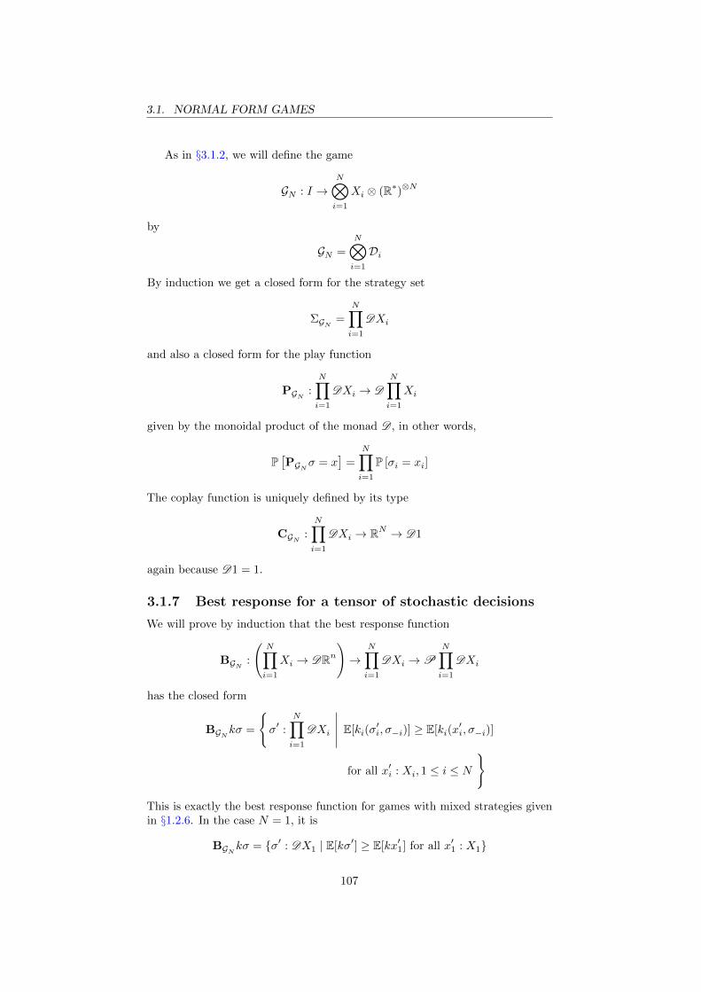
3.1. NORMAL FORM GAMES
As in §3.1.2, we will define the game
GN : I →N⊗i=1
Xi ⊗ (R∗)⊗N
by
GN =
N⊗i=1
Di
By induction we get a closed form for the strategy set
ΣGN =
N∏i=1
DXi
and also a closed form for the play function
PGN :
N∏i=1
DXi → DN∏i=1
Xi
given by the monoidal product of the monad D , in other words,
P[PGNσ = x
]=
N∏i=1
P [σi = xi]
The coplay function is uniquely defined by its type
CGN :
N∏i=1
DXi → RN → D1
again because D1 = 1.
3.1.7 Best response for a tensor of stochastic decisions
We will prove by induction that the best response function
BGN :
(N∏i=1
Xi → DRn)→
N∏i=1
DXi →PN∏i=1
DXi
has the closed form
BGNkσ =
{σ′ :
N∏i=1
DXi
∣∣∣∣∣ E[ki(σ′i, σ−i)] ≥ E[ki(x
′i, σ−i)]
for all x′i : Xi, 1 ≤ i ≤ N
}
This is exactly the best response function for games with mixed strategies givenin §1.2.6. In the case N = 1, it is
BGNkσ = {σ′ : DX1 | E[kσ′] ≥ E[kx′1] for all x′1 : X1}
107

3.1. NORMAL FORM GAMES
which holds by definition.Note that from this point, we begin to abuse notation by leaving the Kleisli
extension of D implicit. This is standard practice in mathematics, where forexample an ordinary non-stochastic function f can be applied to a randomvariable α, resulting in a random variable fα.
By the same reasoning as in §3.1.3, the condition
(σ′−(N+1), σ′N+1) ∈ BGN+1
k(σ−(N+1), σN+1)
is equivalent to the pair of conditions
σ′−(N+1) ∈ BGNk⊗σN+1σ−(N+1)
andσ′N+1 ∈ BDN+1
kσ−(N+1)⊗σN+1
The former, by the inductive hypothesis, is equivalent to the claim that for all1 ≤ i ≤ N and x′i : Xi,
E[(k⊗σN+1)i((σ
′−(N+1))i, (σ−(N+1))−i)] ≥ E[(k⊗σN+1
)i(x′i, (σ−(N+1))−i)]
The latter, by definition of DN+1, is equivalent to the claim that for all deviationsx′N+1 : XN+1,
E[kσ−(N+1)⊗σ′N+1] ≥ E[kσ−(N+1)⊗x
′N+1]
We must prove that for all 1 ≤ i ≤ N + 1 and x′i : Xi,
E[ki(σ′i, σ−i)] ≥ E[ki(x
′i, σ−i)]
In order to obtain this from the inductive hypothesis, it remains to provethat
(k⊗σN+1)i(x
′i, (σ−(N+1))−i) = ki(x
′i, σ−i)
for 1 ≤ i ≤ N and x′i : Xi, and
kσ−(N+1)⊗x′N+1 = kN+1(σ−(N+1), x
′N+1)
for x′N+1 : XN+1. Continuing to abuse notation, for the former we can say that
(k⊗σN+1)i(x
′i, (σ−(N+1))−i) = (k−(N+1))i(x
′i, (σ−(N+1))−i, σN+1)
= ki(x′i, σ−i)
and similarly,kσ−(N+1)⊗x
′N+1 = kN+1(σ−(N+1), x
′N+1)
holds by definition. More carefully, both sides of the former are given by
P[ki(x
′i, σ−i) = ui
]=
∑u−i:R
N
x−i:∏j 6=iXj
∏j 6=i
P[σj = xj
] · P [k(x′i, x−i) = u]
and the latter by
P[kN+1(σ−(N+1), x
′N+1) = uN+1
]=
∑u−(N+1):R
N
x−(N+1):∏Nj=1Xj
N∏j=1
P[σj = xj
] · P [k(x−(N+1), x′N+1) = u
]
108

3.2. EXTENSIVE FORM
3.2 Extensive form
3.2.1 Discussion
In §3.1 we showed that normal form games can be translated into abstract scalarsin GameN (Set) or GameN (SRel) in a way that preserves the pure or mixedstrategies and Nash equilibria, respectively. In this chapter, we will focus ontranslating extensive form games into abstract scalars in GameSP (Set), whilepreserving pure strategies and subgame perfect equilibria. GameSP (Set) isthe category whose composition operation is SP -composition, defined in §2.2.4,which is proved in the appendix to be symmetric premonoidal.
We give a complete proof for the case of sequential games, that is, perfectinformation games in which the type of choices of a player may not depend onthe values of previous choices (see §1.3.1 and §1.3.4). In §3.2.7 we additionallydiscuss the representation of imperfect information. Giving a general translationof an arbitrary extensive form game into an abstract scalar of GameSP (Set)would be more work, and is left for the future.
We will see in §3.3.7 that using the same method to translate extensiveform games with mixed strategies into GameSP (SRel) goes wrong, in the sensethat it gives an implausible solution concept, and that the most fundamentaldefinitions in §2.1 and §2.2 will need to be changed as a result. This is why werestrict to pure strategies in this chapter.
This section is, technically speaking, the most difficult of this thesis, with§3.2.4 and §3.2.5 being particularly dense. Verifying these proofs is made moredifficult by the fact that it is necessary for readability to leave many isomorphismsof sets implicit, such as when using the notation (x′i, x−i) for unilateral deviation.3
An implementation in a proof assistant such as Coq would be useful, and will beeven more important when scaling this style of proof beyond such simple typesof games as are considered in this thesis.
3.2.2 Composition with perfect information
We will begin with a sequence of decisions
Di :
i−1⊗j=1
Xj → Xi ⊗ R∗
in GameSP (Set). The ith decision represents a player who observes the firsti− 1 choices. Note that since the empty tensor is the identity, the first of theseis D1 : I → X1 ⊗ R∗. We will define a game
GN : I →N⊗i=1
Xi ⊗ (R∗)⊗N
which behaves like their perfect information composition, by induction on N .Like for simultaneous games, the base case is G1 = D1.
For the inductive step, we are given GN and DN+1, and we must produceGN+1. In this game, GN must play first, and then DN+1 must play observing
3These are precisely the isomorphisms that need to be explicit in Haskell code, as discussed
in §0.2.
109

3.2. EXTENSIVE FORM
the choices of GN . However, the choices of GN must also be preserved in theoutput of GN+1, and hence must be copied in parallel with DN+1. The stringdiagram to keep in mind is
GN DN+1
N⊗i=1
Xi
XN+1
R⊗N
R
N⊗i=1
Xi
However, because GameSP (Set) is not a monoidal category we do not actuallyhave a string diagram language, and so the real definition is given by the algebraicterm below.
We will translate this diagram into monoidal category notation in stages.The decision is
DN+1 :
N⊗i=1
Xi → XN+1 ⊗ R∗
To add the string above it we tensor with the identity
N⊗i=1
Xi ⊗DN+1 :
N⊗i=1
Xi ⊗N⊗i=1
Xi →N+1⊗i=1
Xi ⊗ R∗
The copying node is the computation
∆∏Ni=1Xi
:
N⊗i=1
Xi →N⊗i=1
Xi ⊗N⊗i=1
Xi
The top-right part of the diagram is therefore(N⊗i=1
Xi ⊗DN+1
)◦SP ∆∏N
i=1Xi:
N⊗i=1
Xi →N+1⊗i=1
Xi ⊗ R∗
Before the lower-right crossing, we can tensor with the lower R⊗N -labelledcontravariant string to get((
N⊗i=1
Xi ⊗DN+1
)◦SP ∆∏N
i=1Xi
)⊗ (R∗)⊗N
110
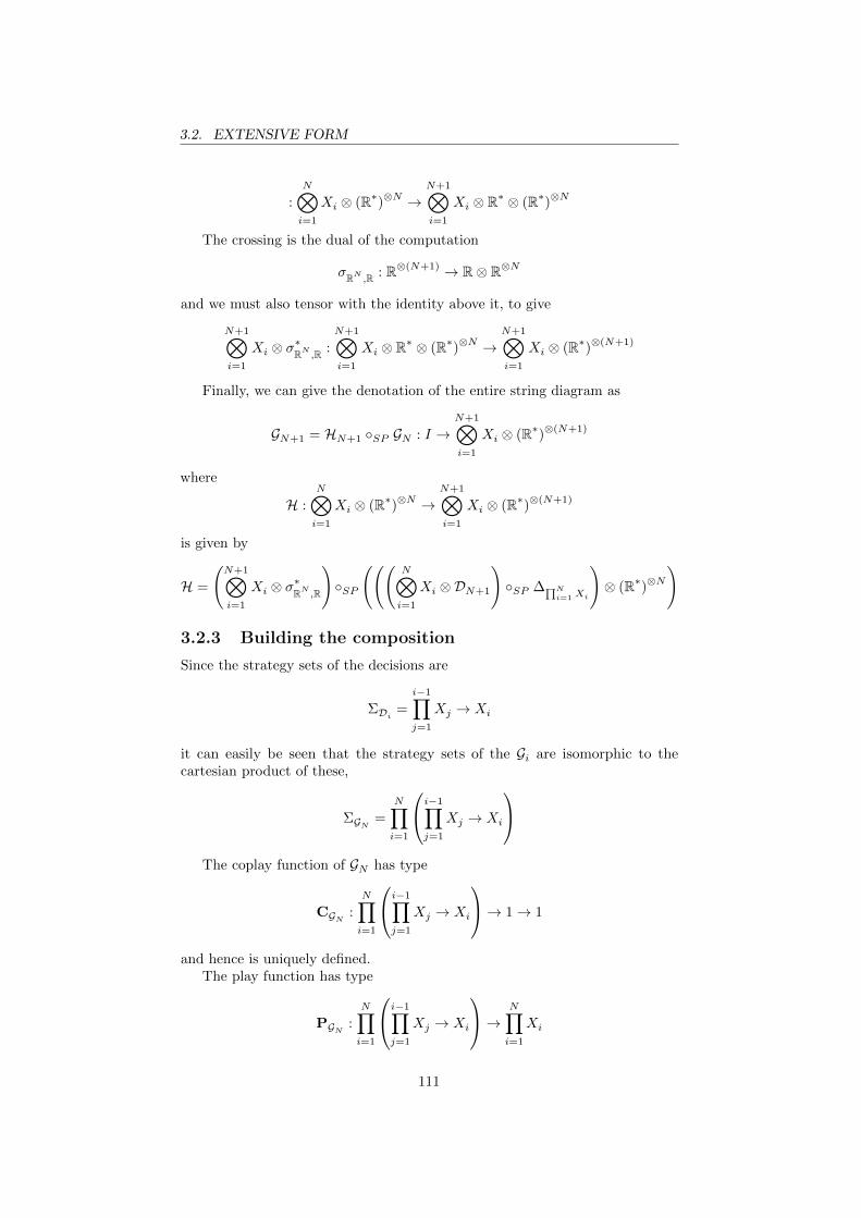
3.2. EXTENSIVE FORM
:
N⊗i=1
Xi ⊗ (R∗)⊗N →N+1⊗i=1
Xi ⊗ R∗ ⊗ (R∗)⊗N
The crossing is the dual of the computation
σRN ,R : R⊗(N+1) → R⊗ R⊗N
and we must also tensor with the identity above it, to give
N+1⊗i=1
Xi ⊗ σ∗RN ,R :
N+1⊗i=1
Xi ⊗ R∗ ⊗ (R∗)⊗N →N+1⊗i=1
Xi ⊗ (R∗)⊗(N+1)
Finally, we can give the denotation of the entire string diagram as
GN+1 = HN+1 ◦SP GN : I →N+1⊗i=1
Xi ⊗ (R∗)⊗(N+1)
where
H :
N⊗i=1
Xi ⊗ (R∗)⊗N →N+1⊗i=1
Xi ⊗ (R∗)⊗(N+1)
is given by
H =
(N+1⊗i=1
Xi ⊗ σ∗RN ,R
)◦SP
(((N⊗i=1
Xi ⊗DN+1
)◦SP ∆∏N
i=1Xi
)⊗ (R∗)⊗N
)
3.2.3 Building the composition
Since the strategy sets of the decisions are
ΣDi =
i−1∏j=1
Xj → Xi
it can easily be seen that the strategy sets of the Gi are isomorphic to thecartesian product of these,
ΣGN =
N∏i=1
i−1∏j=1
Xj → Xi
The coplay function of GN has type
CGN :
N∏i=1
i−1∏j=1
Xj → Xi
→ 1→ 1
and hence is uniquely defined.The play function has type
PGN :
N∏i=1
i−1∏j=1
Xj → Xi
→ N∏i=1
Xi
111

3.2. EXTENSIVE FORM
We will prove that PGN = P is the play function for sequential games introducedin §1.3.4. Explicitly, we will prove that
(PGNσ)i = σi((PGNσ)1, . . . , (PGNσ)i−1)
for all 1 ≤ i ≤ N . This should be compared to the defining equation of the playfunction in §1.3.4. In the base case G1 = D1, the play function is by definition
(PD1σ)1 = PD1
σ = σ = σ1
which satisfies the equation.For the inductive step, we need to show that
PGN+1σ = (x, σN+1x)
where x = PGNσ−(N+1). Since
PGN+1σ = PHN+1
σN+1 ◦PGNσ−(N+1)
it suffices to prove that
PHN+1σN+1x = (x, σN+1x)
To begin with, we note that
P⊗Ni=1Xi⊗σ
∗RN,R
= id∏Ni=1Xi
and so
PHN+1σN+1 = P(
(⊗Ni=1Xi⊗DN+1)◦SP∆∏N
i=1 Xi
)⊗(R∗)⊗N
σN+1
= P(⊗Ni=1Xi⊗DN+1)◦SP∆∏N
i=1 Xi
σN+1
Then
P(⊗Ni=1Xi⊗DN+1)◦SP∆∏N
i=1 Xi
σN+1x = P⊗Ni=1Xi⊗DN+1
σN+1
(P∆∏N
i=1 Xi
x
)= P⊗N
i=1Xi⊗DN+1σN+1
(∆∏N
i=1Xix)
= P⊗Ni=1Xi⊗DN+1
(x, x)
=(P⊗N
i=1Xix,PDN+1
σN+1x)
= (x, σN+1x)
Having proved this, we have
(PGN+1σ)i =
{(PGNσ−(N+1))i if i ≤ NσN+1(PGNσ−(N+1)) if i = N + 1
For i ≤ N , the inductive hypothesis gives
(PGN+1σ)i = (PGNσ−(N+1))i
= (σ−(N+1))i((PGNσ−(N+1))1, . . . , (PGNσ−(N+1))i−1)
= σi((PGN+1σ)1, . . . , (PGN+1
σ)i−1)
112

3.2. EXTENSIVE FORM
and for i = N + 1,
(PGN+1σ)N+1 = σN+1(PGNσ−(N+1))
= σN+1((PGNσ−(N+1))1, . . . , (PGNσ−(N+1))N )
= σN+1((PGN+1σ)1, . . . , (PGN+1
σ)N )
3.2.4 Best response for the composition
We will now prove that our best response function
BGN :
(N∏i=1
Xi → RN)→ ΣGN →PΣGN
where
ΣGN =
N∏i=1
i−1∏j=1
Xj → Xi
is such that BGNkσ is the set of all σ′ : ΣGN such that, for all players 1 ≤ i ≤ Nand all partial plays x = x1, . . . , xi−1 of length i− 1, and all possible deviationsxi : Xi, we have
(U kx σ(σ′ix))i ≥ (U k
x σxi)i
where U kx is the unilateral deviation operator for sequential games, defined in
§1.3.5.The proof is again by induction on N . In the base case we have N = 1 and
we need only check i = 1 with the empty partial play and some deviation x1 : X1.Then
(U kσσ′)1 = kσ′
and(U kσx1)1 = kx1
and we are done, because by definition BG1 = BD1takes k : X1 → R and σ : X1
to the set of all σ′ : X1 such that
kσ′ ≥ kx′
for all x′ : X1
Next, by the definition of composition,
BGN+1kσ = BGNkσN+1◦σ−(N+1)
×⋂σ′:ΣG
BHN+1(PGNσ
′, k)σN+1
For BGN+1kσ to contain some σ′, it must be that
σ′−(N+1) ∈ BGNkσN+1◦σ−(N+1)
and for all σ′′−(N+1),
σ′N+1 ∈ BHN+1(PGNσ
′′−(N+1), k)σN+1
113

3.2. EXTENSIVE FORM
The first condition, by the inductive hypothesis, is equivalent to the claimthat for all 1 ≤ i ≤ N , partial plays x = x1, . . . , xi−1 :
∏j<iXj and devations
xi : Xi,
(UkσN+1◦x σ−(N+1)((σ
′−(N+1))ix))i ≥ (U
kσN+1◦x σ−(N+1)xi)i
We claim that there is an equality of continuations
UkσN+1◦x σ−(N+1) = π−(N+1) ◦U k
x σ : Xi → RN
which immediately gives us the inductive hypothesis for N + 1 when 1 ≤ i ≤ N .To show this, by definition
kσN+1◦ :
N∏j=1
Xj → RN
is given bykσN+1◦x = k−(N+1)(x, σN+1x)
Now we have
UkσN+1◦x σ−(N+1)xi = kσN+1◦(ν
σ−(N+1)x,xi )
= k−(N+1)(νσ−(N+1)x,xi , σN+1(ν
σ−(N+1)x,xi ))
where ν is defined in §1.3.5, because by definition
U kx σxi = k(νσx,xi)
Therefore it suffices to prove that
νσx,xi = (νσ−(N+1)x,xi , σN+1(ν
σ−(N+1)x,xi ))
By definition(νσx,xi)N+1 = σN+1((νσx,xi)1, . . . , (ν
σx,xi
)N )
so it suffices to prove that
(νσx,xi)j = (νσ−(N+1)x,xi )j
for 1 ≤ j ≤ N . This is easily proved by strong induction on j.
3.2.5 Best response for the composition, continued
We now return to the second condition for
σ′ ∈ BGN+1kσ
namely that for all σ′′−(N+1) : ΣGN ,
σ′N+1 ∈ BHN+1(PGNσ
′′−(N+1), k)σN+1
We claim that this is equivalent to
σ′N+1 ∈ BDN+1(PGNσ
′′−(N+1), k
′)σN+1
114

3.2. EXTENSIVE FORM
where k′ : XN+1 → R is given by
k′xN+1 = kN+1(PGNσ′′−(N+1), xN+1)
We will prove the slightly more general claim where PGNσ′′−(N+1) is replaced
with a general play x−(N+1). To begin, since⊗N+1
i=1 Xi ⊗ σ∗RN ,R is strategically
trivial,
BHN+1(x−(N+1), k)σN+1
= B((⊗Ni=1Xi⊗DN+1)◦SP∆∏N
i=1 Xi
)⊗(R∗)⊗N
(x−(N+1), k∗◦)σN+1
where
k∗◦ :
N+1∏i=1
Xi → RN+1
is the extended continuation defined in §2.2.3, given explicitly by
k∗◦x = C⊗N+1i=1 Xi⊗σ
∗RN,R
(x, k(P⊗N+1i=1 Xi⊗σ
∗RN,R
x))
= σRN ,R(k(id∏Ni=1Xi
x))
= (kN+1x, k−(N+1)x)
Next, because the identity on (R∗)⊗N is strategically trivial,
B((⊗Ni=1Xi⊗DN+1)◦SP∆∏N
i=1 Xi
)⊗(R∗)⊗N
(x−(N+1), k∗◦)σN+1
= B(⊗Ni=1Xi⊗DN+1)◦SP∆∏N
i=1 Xi
(x−(N+1), (k∗◦)1)σN+1
where(k∗◦)1x = kN+1x
Therefore
B(⊗Ni=1Xi⊗DN+1)◦SP∆∏N
i=1 Xi
(x−(N+1), kN+1)σN+1
= B⊗Ni=1Xi⊗DN+1
(P∆∏Ni=1 Xi
x−(N+1), kN+1)σN+1
= B⊗Ni=1Xi⊗DN+1
(∆∏Ni=1Xi
x−(N+1), kN+1)σN+1
= B⊗Ni=1Xi⊗DN+1
((x−(N+1), x−(N+1)), kN+1)σN+1
= BDN+1(x−(N+1), (kN+1)∗(x−(N+1))⊗)σN+1
where
(kN+1)∗(x−(N+1))⊗xN+1 = kN+1(P⊗Ni=1Xi
x−(N+1), xN+1)
= kN+1(x−(N+1), xN+1)
= k′xN+1
for the definition of k′ given earlier.
115

3.2. EXTENSIVE FORM
Now, by definition of BDN+1, the condition
σ′N+1 ∈ BDN+1(PGNσ
′′−(N+1), k
′)σN+1
is equivalent tok′(σ′N+1(PGNσ
′′−(N+1))) ≥ k
′xN+1
for all xN+1 : XN+1, which is
kN+1(PGNσ′′−(N+1), σ
′N+1(PGNσ
′′−(N+1))) ≥ kN+1(PGNσ
′′−(N+1), xN+1)
It remains to show that this, universally quantified over σ′′−(N+1) : ΣGN , impliesthe remaining case of the inductive hypothesis for N + 1, namely that for allpartial plays x = x1, . . . , xN :
∏Nj=1Xj and deviations xN+1 : XN+1,
(U kx σ(σ′N+1x))N+1 ≥ (U k
x σxN+1)N+1
Notice that
(U kx σxN+1)N+1 = kN+1(νσx,xN+1
) = kN+1(x, xN+1) = k′xN+1
so we must showkN+1(x, σ′N+1x) ≥ kN+1(x, xN+1)
for all partial plays x.Given such an x, we take the strategy profile
(σ′′−(N+1))ix′ = xi
which ignores its observation, and simply plays the move from x. We claim thatPGNσ
′′ = x. Using the characterisation of PGN in §3.2.3, for each 1 ≤ i ≤ N wehave
(PGNσ′′−(N+1))i = (σ′′−(N+1))i((PGNσ
′′−(N+1))1, . . . , (PGNσ
′′−(N+1))i−1)
= xi
This completes the proof.
3.2.6 Information sets
Information sets are used in [vNM44] to give a general theory of imperfectinformation, including games that are intermediate between sequential andsimultaneous. In general, a player may be able to observe partial informationabout another player’s earlier move. That is, they may be able to distinguishsome pairs of moves, but not others.
For simplicity, we will begin with a concrete two-player game. Suppose theset of moves for the first player is X = {x1, x2, x3} and the set of moves for thesecond player is Y = {y1, y2}. The game tree for this game is
116

3.2. EXTENSIVE FORM
x1 x2 x3
y1 y2 y1 y2 y1 y2
An information set for the second player is simply a partitioning of X, thatis to say, an equivalence relation on X. The intention is that two elements ofX that are in the same equivalence class cannot be distinguished by the secondplayer, whereas elements in different equivalence classes can be. In this example,the dashed line is the usual notation for specifying that two nodes are in thesame equivalence class. Thus, our partitioning of X is X/∼ = {{x1, x2}, {x3}}.
For simplicity, we will focus on pure strategies, although sequential equilibrium[LBS08] is a more common solution concept for games with nontrivial informationsets (and see §3.3.7). The informal condition that the second player cannotdistinguish between x1 and x2 can be interpreted formally as a restriction on theallowed strategies, namely that every strategy for player 2 must be compatiblewith the equivalence relation. Thus, a function σ2 : X → Y is an allowed strategyfor player 2 iff σ2x1 = σ2x2. This is equivalent to saying that σ2 is actually afunction σ2 : X/∼ → Y . The set of strategies of this game, therefore, is
Σ = X × (X/∼ → Y )
The general definition of a subgame perfect equilibrium, including withnontrivial information sets, is a strategy that induces a Nash equilibrium onevery subgame. For this two-stage game, this is the same as a fixpoint of thebest response function B : Σ → PΣ, where B(σ1, σ2) is the set of all (σ′1, σ
′2)
satisfying the two conditions4
q1(σ′1, σ2[σ′1]) ≥ q1(x′, σ2[x′])
for all x′ : X, andq2(x′, σ′2[x′]) ≥ q2(x′, y′)
for all x′ : X and y′ : Y . Equivalently, we can give the two conditions as
σ′1 = arg maxx′:X
q1(x′, σ2[x′])
and for all x′ : X,σ′2[x′] = arg max
y′:Y
q2(x′, y′)
4The notation [x] refers to the information set to which x belongs.
117

3.2. EXTENSIVE FORM
3.2.7 Imperfect information via open games
We will end this section by taking a more general two player game involvingimperfect information, and showing how it can be formalised in GameSP (Set).The sets of moves are X and Y , and we have an equivalence relation ∼ on X. Astrategy profile is a pair (σ1, σ2) : X × (X/∼ → Y ). The definition of subgameperfect equilibrium is as before.
Intuitively, we use the string diagram
D1 π∼
D2
X
Y
R
R
XX
X/∼
where π∼ : X → X/∼ is the projection onto information sets, π∼x = [x].However, as before, this cannot be formalised because GameSP (Set) is notmonoidal. This should be compared to the string diagrams in §2.3.10 and §3.2.2,which denote perfect information games in which ∼ is the identity relation, andso π∼ is the identity on X. Notice how we can explicitly see that the informationflowing from D1 to D2 passes through the projection π∼, where it is partiallyhidden.
Since most of the analysis is the same as for the perfect information case, wewill focus on the sub-diagram
X
X
Y
R
π∼ D2
X/∼
which is given algebraically by
G = (X ⊗ (D2 ◦SP π∼)) ◦SP ∆X : X → X ⊗ Y ⊗ R∗
118

3.3. SOLVABLE GAMES
The set of strategy profiles is ΣG = X/∼ → Y , with play function
PGσx = (x, σ[x])
The best response function
BG : X × (X × Y → R)→ ΣG →PΣG
is calculated as
BG(h, k)σ = BX⊗(D2◦SPπ∼)((h, h), k)σ
= BD2◦SPπ∼(h, k′)σ
= BD2([h], k′)σ
where k′y = k(h, y).Since BD2
is a utility-maximising decision, this is
BG(h, k)σ = {σ′ : X/∼ → Y | k(h, σ[h]) ≥ k(h, y′) for all y′ : Y }
and the condition can be equivalently written
σ[h] = arg maxy′:Y
k(h, y′)
This corresponds exactly to the second condition for the best response functionin §3.2.6.
3.3 Solvable games
3.3.1 Discussion
In this section we will introduce a suitable solution concept for open games,called solvability. Although the best response function of a game contains allof the information needed to define equilibria, it does not seem to be directlyusable as a solution concept, because there is nothing that corresponds directlyto an ‘equilibrium of an open game’. A solution of a game, on the other hand, isdefined in terms of the best response function and can be directly read as ananalogue of Nash or subgame perfect equilibria for open games.
The solvability of a game should be seen as a witness for an existence theorem.This is because a solution of an open game implies the existence of equilibria fora class of closed games obtained by varying its continuation, that is, for a classof games whose outcome function varies. For example, as mentioned in §3.3.6there is a single open game whose solvability is equivalent to the Nash existencetheorem for bimatrix games (of fixed size).
The ultimate aim is to show that solvability is respected by the categoricaloperations used to construct games, which will allow us to prove existencetheorems by structural induction, and compute equilibria recursively.5 In §3.3.4we will show that when applied to categorical composition this yields somethingakin to backward induction in classical game theory, and thereby connect solutionswith selection functions. In §3.3.6 and §3.3.7, we will discuss how solvabilitybehaves with respect to tensor products, which is more subtle and is ongoingwork.
5Anything less would shackle the power of compositional game theory.
119

3.3. SOLVABLE GAMES
3.3.2 The definition of solvability
Let G : X ⊗ S∗ → Y ⊗ R∗ be a game in GameN (C) or GameSP (C). We willcall G solvable if, for every continuation k : homC(Y,R), there exists a strategyσ : ΣG , such that for all histories h : homC(I,X), we have σ ∈ BG(h, k)σ.
A solution of G is a function6 s : homC(Y,R)→ ΣG such that sk is a fixpointof BG(h, k) for all contexts (h, k) : homC(I,X)× homC(Y,R). By the axiom ofchoice, a game is solvable iff it has a solution.
A first technical issue with solvability is that it is not ‘aware’ of coutility,because the definition of solvability of G does not refer to S or CG . Consequently,the solutions of
f
G
X
S′
Y
RS
are independent of the computation f : S → S′.Notice that all strategically trivial games (§2.2.11) are solvable. Take a
strategically trivial game G : X ⊗ S∗ → Y ⊗ R∗, so we have ΣG = 1, and forevery h : homC(I,X) and k : homC(Y,R) we have
∗ ∈ BG(h, k)∗
Then the unique function s : homC(Y,R)→ ΣG is trivially a solution.The following is a simple but useful way to obtain new solvable games from
old. Let G : X ⊗ S∗ → Y ⊗ R∗ be solvable, and let f : R′ → R ⊗ T be acomputation. Then
G
f
X Y
R′
S
T
R
is also solvable. When solutions are connected with selection functions in §3.3.5,this is analogous to modifying the outcome type of a selection function (§1.1.8).Algebraically, the game denoted by this string diagram is
(Y ⊗ f∗) ◦SP (G ⊗ T ∗) : X ⊗ S∗ ⊗ T ∗ → Y ⊗R′∗
(and the same holds if ◦SP is replaced with ◦N .) It is obtained from G bycomposing and tensoring with strategically trivial games, and so
Σ(Y⊗f∗)◦SP (G⊗T∗) = ΣG
6A strategy relative to a continuation.
120

3.3. SOLVABLE GAMES
Its best response function is
B(Y⊗f∗)◦SP (G⊗T∗) : homC(I,X)× homC(Y,R′)→ ΣG →PΣG
given byB(Y⊗f∗)◦SP (G⊗T∗)(h, k)σ = BG(h, k′)σ
where
k′ : Yk−→ R′
f−→ R⊗ T π1−→ R
Let k : homC(Y,R) be a continuation for (Y ⊗f∗)◦SP (G⊗T ∗). By the solvabilityof G with the continuation k′, we have σ : ΣG such that, for all h : homC(I,X),
σ ∈ BG(h, k′)σ
Thus σ ∈ B(Y⊗f∗)◦SP (G⊗T∗)(h, k)σ, as required.
3.3.3 Solvable decisions
We will now provide our first nontrivial examples of a solvable games, namelythe decisions over Set defined in §2.1.8 that maximise with respect to a rationalpreference relation � on a set R. These are
D : X → Y ⊗R∗
defined by the rationality function
R : X × (Y → R)→P(X → Y )
given byR(x, k) = {σ : X → Y | k(σx) � ky for all y : Y }
We will prove that this decision is solvable, if Y is finite.Let k : Y → R be a continuation. Then since Y is finite and � is a rational
preference relation there is some y : Y for which ky is maximal. Pick theconstant7 strategy σ : X → Y given by σx = y. Then for all h : X we haveσ ∈ BD(h, k)σ because for all y′ : Y we have
k(σx) = ky � ky′
In GameSP (Set) we can prove a stronger ad-hoc result, namely that
D
X
X
Y
R
7The fact that we can use a constant strategy here seems to be related to the problem
discussed in §3.3.7.
121

3.3. SOLVABLE GAMES
is also solvable. Algebraically, this game is (X ⊗D) ◦SP ∆X , which is obtainedfrom D by tensoring and composing with strategically trivial games. Thus, thestrategy set is
Σ(X⊗D)◦SP∆X= ΣD = X → Y
Its best response function, by similar reasoning as in §3.2.4, is
B(X⊗D)◦SP∆X(h, k)σ = {σ′ : X → Y | σ′ ∈ BD(h, k′)σ}
where k′ : Y → R is given by k′y = k(h, y). Explicitly, this is
B(X⊗D)◦SP∆X(h, k)σ = {σ′ : X → Y | k(h, σ′h) � k(h, y) for all y : Y }
Now let k : X × Y → R be a continuation for (X ⊗ D) ◦SP ∆X . Define astrategy σ : X → Y by
σx = arg maxy:Y
k(x, y)
where arg max picks some y that attains the �-maximum. Then for every historyh : X we have
k(h, σx) � k(h, y)
by construction, and hence σ ∈ B(X⊗D)◦SP∆X(h, k)σ.
3.3.4 Backward induction for open games
We will now prove that solvable games are closed under SP -composition. Theproof of this result amounts to backward induction, just as does the productof selection functions (§1.3.6). This is the main piece of evidence thus far thatsolvable games are mathematically natural.
Suppose we have games
G H
X Z
RT
Y
S
with solutionssG : homC(Y, S)→ ΣG
sH : homC(Z,R)→ ΣH
We define sH◦SPG : homC(Z,R)→ ΣG × ΣH by
sH◦SPGk = (sGksHk◦, sHk)
where ksHk◦ : homC(Y, S) is the extended continuation defined in §2.2.3. Wemust prove that sH◦SPG is a solution of H ◦SP G.
Let (h, k) : homC(I,X) × homC(Z,R) be a context for H ◦SP G. We mustprove that
sH◦SPGk ∈ BH◦SPG(h, k)(sH◦SPGk)
This unwinds to the two conditions
sGksHk◦ ∈ BG(h, ksHk◦)(sGksHk◦)
122
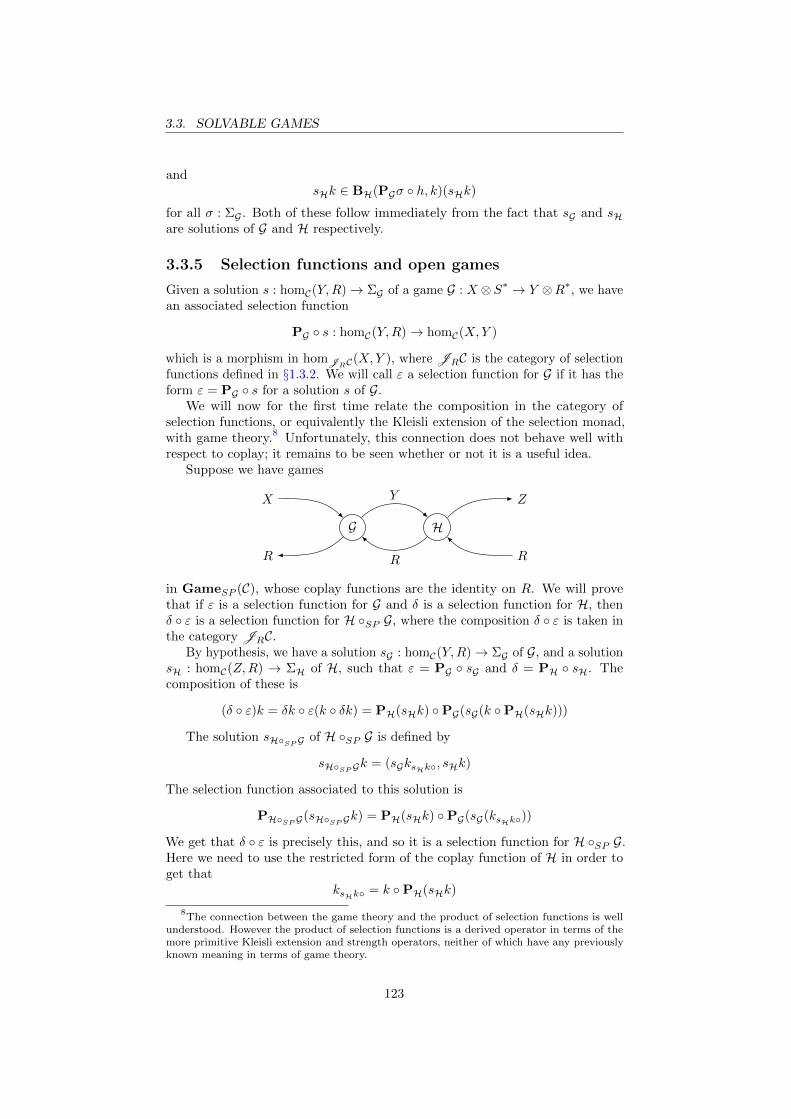
3.3. SOLVABLE GAMES
andsHk ∈ BH(PGσ ◦ h, k)(sHk)
for all σ : ΣG . Both of these follow immediately from the fact that sG and sHare solutions of G and H respectively.
3.3.5 Selection functions and open games
Given a solution s : homC(Y,R)→ ΣG of a game G : X ⊗S∗ → Y ⊗R∗, we havean associated selection function
PG ◦ s : homC(Y,R)→ homC(X,Y )
which is a morphism in homJRC(X,Y ), where JRC is the category of selectionfunctions defined in §1.3.2. We will call ε a selection function for G if it has theform ε = PG ◦ s for a solution s of G.
We will now for the first time relate the composition in the category ofselection functions, or equivalently the Kleisli extension of the selection monad,with game theory.8 Unfortunately, this connection does not behave well withrespect to coplay; it remains to be seen whether or not it is a useful idea.
Suppose we have games
G H
X Z
RR
Y
R
in GameSP (C), whose coplay functions are the identity on R. We will provethat if ε is a selection function for G and δ is a selection function for H, thenδ ◦ ε is a selection function for H ◦SP G, where the composition δ ◦ ε is taken inthe category JRC.
By hypothesis, we have a solution sG : homC(Y,R)→ ΣG of G, and a solutionsH : homC(Z,R) → ΣH of H, such that ε = PG ◦ sG and δ = PH ◦ sH. Thecomposition of these is
(δ ◦ ε)k = δk ◦ ε(k ◦ δk) = PH(sHk) ◦PG(sG(k ◦PH(sHk)))
The solution sH◦SPG of H ◦SP G is defined by
sH◦SPGk = (sGksHk◦, sHk)
The selection function associated to this solution is
PH◦SPG(sH◦SPGk) = PH(sHk) ◦PG(sG(ksHk◦))
We get that δ ◦ ε is precisely this, and so it is a selection function for H ◦SP G.Here we need to use the restricted form of the coplay function of H in order toget that
ksHk◦ = k ◦PH(sHk)
8The connection between the game theory and the product of selection functions is well
understood. However the product of selection functions is a derived operator in terms of themore primitive Kleisli extension and strength operators, neither of which have any previouslyknown meaning in terms of game theory.
123

3.3. SOLVABLE GAMES
rather than (in pure strategies)
ksHk◦y = CH(sHk)(y, k(PH(sHk)y))
This provides us with a high level way to think about solvability. Given anobject R of C, we consider the subcategory GameSP (C, R) whose objects areof the form X ⊗ R∗ for X an object of C, and whose morphisms are solvablegames whose coplay function is constant. Then a (compatible) choice of solutionsG for each game G defines a functor F : GameSP (C, R)→JRC whose actionon objects is F (X ⊗R∗) = X and on morphisms is FG = PG ◦ sG . Although itis possible to do a certain amount of game theory in GameSP (C, R) when R issuitably chosen, it is unlikely that this way of thinking has enough benefit tooffset the restriction of not having coplay available, which limits compositionalityin practice. One way in which this is useful, however, is to understand therelationship between selection functions and open games.
3.3.6 Tensor does not preserve solvability
In general, the class of solvable games is not closed under tensor. This is ahigh level way of saying that simultaneous games do not have equilibria forevery solution concept, and in particular they do not have pure strategy Nashequilibria.
We will give a counterexample using matching pennies, which is the simplestgame with no pure strategy equilibrium. In this game two players each simulta-neously choose H (‘heads’) or T (‘tails’). If both players make the same choicethen player 1 wins, and if the choices are different player 2 wins. This game hasno pure strategy Nash equilibrium, because when playing a strategy in whichboth choices are the same player 2 has incentive to deviate, and when playinga strategy in which the choices are different player 1 has incentive to deviate.(This game has a unique mixed strategy equilibrium, in which both players mixwith equal probability.)
We will formalise this game by working in GameSP (Set). Let X = {H,T},and let R be the poset {0 ≺ 1}, where 1 indicates winning and 0 indicates losing.The maximising decision
D : I → X ⊗R∗
was proved to be solvable in §3.3.3.We will now prove that the tensor product D ⊗D is not solvable. To show
this, we must exhibit a particular continuation k : X ×X → R × R with theproperty that
BD⊗Dk : X ×X →P(X ×X)
has no fixpoints. This is equivalent to saying that the game with outcomefunction k has no pure strategy Nash equilibrium. Therefore, we take k to bethe outcome function of matching pennies, namely
k(x, y) =
{(1, 0) if x = y
(0, 1) if x 6= y
This givesBD⊗Dk(x, y) = {(y, x)}
124

3.3. SOLVABLE GAMES
where · : X → X interchanges H and T . This function indeed has no fixpoint.If we reasoned in GameSP (SRel) instead of GameSP (Set) then this does
not happen: by Nash’s theorem, the tensor product of finitely many decisionsover finite sets of choices in GameSP (SRel) is solvable.
3.3.7 Failure of compositional Nash’s theorem
An early motivation for introducing solvable games, besides connecting opengames and selection functions (§3.3.5), was to prove a suitable generalisation ofNash’s theorem for open games. The fact that solvable games are closed undercomposition (§3.3.4), but fail to be closed under tensor because pure strategyNash equilibria need not exist (§3.3.6), strongly suggests the conjecture that inGameSP (SRel), all freely generated games are solvable.
This fails, however, because it is not the case that arbitrary solvable gamesin GameSP (SRel) are closed under tensor product. This appears to result froma much deeper issue with the definitions in §2.1 and §2.2. In §3.1 it was shownthat normal form games with mixed strategies Nash equilibria can be faithfullyrepresented by open games, and similarly for extensive form games and purestrategy subgame perfect equilibria in §3.2. However, if the two are combined, weend up with a uselessly implausible solution concept.9 The previous conjecture,that all freely generated games are solvable, can be taken as a requirement for arepaired theory.
We will end with a specific counterexample to the conjecture. Consider thegame in GameSP (SRel) denoted by
D1 D2 q
X
XX
R
R
or G = q ◦SP (X ⊗ D2 ⊗ R∗) ◦SP D1, where X = {H,T}. D2 is an ordinarydecision that maximises expected utility, and D1 also maximises expected utilitybut chooses a pair from X ×X with a mixed strategy. The strategically trivialgame q (which could be decomposed into computations and counits) implementsthe outcome function, which is again that of matching pennies. Specifically, the
9In retrospect this is unsurprising, because the equivalently naive generalisation of mixed
strategies to extensive form in classical game theory also fails. The standard solution concept inthat situation is sequential equilibrium [LBS08], which involves beliefs (probability distributionson information sets giving finer information about the position in the game tree), that undergoBayesian updating. Because open games are inherently dynamic games, a repaired theoryof open games with mixed strategies must similarly have Bayesian reasoning built into thedefinitions.
125

3.3. SOLVABLE GAMES
coplay function Cq : X ×X → D(R× R) is given by
Cq(x, y) =
{δ(0, 1) if x = y
δ(1, 0) if x 6= y
where δ is the unit of the monad D (see §2.1.3).Since G is a scalar, its best response function has the form
BG : ΣG →PΣG
Despite the fact that we are working over SRel and so we have mixed strategiesavailable, and the fact that G has been built from only expectation-maximisingdecisions, computations and counits using composition and tensor, we will provethat BG has no fixpoints.
The set of strategies is
ΣG = ΣD1× ΣD2
= D(X ×X)× (X → DX)
Geometrically, this is the product of a tetrahedron and a square, and hence isclosed, convex and finite-dimensional, satisfying the hypotheses of the Kakutanifixpoint theorem.
To begin with, since q is strategically trivial we have
BG(∗, ∗)(σ, τ) = B(X⊗D2⊗R∗)◦SPD1
(∗, k)(σ, τ)
where k : X ×X → D(R× R) is the continuation k = ∗∗◦ = q. This is
BD1(∗, kτ◦)σ ×
⋂σ′:D(X×X)
BX⊗D2⊗R∗(PD1
σ′ ◦ ∗, k)τ
We will only need to focus on the second part of this. Since D1 is a decision wehave PD1
σ′ ◦ ∗ = σ′. Then
BX⊗D2⊗R∗(σ′, k)τ = BX⊗D2
(σ′, k1)τ
where k1 : X ×X → DR is given by
k(x1, x2) =
{δ0 if x1 = x2
δ1 if x1 6= x2
The game X ⊗D2 : X ⊗X → X ⊗X ⊗R∗ is essentially the component of Gthat causes the problems. Its best response function is
BX⊗D2(h, k1)τ = BD2
(h1, k′)τ
The continuation k′ = (k1)∗(h1)⊗ : X → DR is given by k′x2 = k1(h1, x2), wherewe are abusing notation as in §3.1.7. Explicitly, using the particular k we defined,
P[k′x2 = 1
]= P [h1 6= x2]
Now using the definition of BD2,
BX⊗D2(h1, k1)τ = {τ ′ : X → DX | E[k′(τ ′h1)] ≥ E[k′x2] for x2 = H,T}
126

3.3. SOLVABLE GAMES
Putting this together, if we had a fixpoint (σ, τ) of BG , then for every possiblehistory h : D(X ×X) we would have
E[k1(h1, τh1)] ≥ E[k1(h1, x2)]
for x2 = H,T . We will now prove that this is impossible.Pick some x1 ∈ supp(τH), so P [τH = x1] > 0. We will take h = δx1 ⊗ δH,
that is, h is the probability distribution with P [h = (x1, H)] = 1. Then
k′(τh1) = k′(τx1) = k1(x1, τH)
and since P [τH = x1] > 0 we have E[k1(x1, τH)] < 1. This means that player 2has incentive to unilaterally deviate to x2 6= x1, which has
E[k′x2] = E[k′(x1, x2)] = 1
127

Conclusion
The future of compositional game theory
This section is partly based on a funding application I wrote, and will sketch aresearch programme about the theory and applications of composing games. Iwill begin with an unreasonably optimistic best-case vision of the future, andwork backwards. This work of speculative fiction is based on long discussionswith Viktor Winschel and Philipp Zahn, mostly in the pub.
Suppose an economist wants to create a mathematical model of some economicsystem, say, a new market. Using her experience as a working economist, sheanalyses the market and divides it into a number of interacting components.Most of these component markets are well known and have been extensivelystudied, and she recognises the last component as behaving similarly to part ofanother market that was recently studied by a colleague.
She opens her software suite and loads these known models, most of whichcome pre-installed, and the last downloaded from a source repository accom-panying her colleague’s research paper. Each of these specifies an open game,whose ports specify how it communicates with an arbitrary environment, whichis graphically represented on the screen by a bead with open strings. Althoughshe has never heard the phrase ‘category theory’ except in a cryptic footnotein the software’s documentation, she draws strings connecting the beads, ina way corresponding to her intuition about how the component markets arecommunicating and influencing each other.
Behind the scenes, the software compiles the string diagram to an intermediaterepresentation, and then to Haskell, which is compiled and optimised by ghc.
The economist begins by specifying a plausible strategy profile, for exampleby drawing a finite state automaton, and then plays the game with the strategyprofile to obtain a plot showing a probability distribution on outcomes. Shetests this against real econometric data and finds that it does not fit the data.She then replaces some parameter in the strategy profile by a variable, and runsan automated optimisation procedure. This takes 30 minutes to complete, andstill does not fit the data well.
By tracing the results through the string diagram, viewing plots of the dataflowing along the intermediate strings, she determines that her colleague’s modelis at fault. She ‘zooms in’ to that model in the editor, seeing visually theinformation flow inside that model. It consists of many standard componentsinteracting, each of which itself can be opened as a string diagram for editing.She manually tunes several quantitative parameters, and qualitatively changesthe logic of the information flow in a few places, in an iterative process, at each
128

3.3. SOLVABLE GAMES
stage comparing the simulation results to the econometric data.Finally, she obtains a model and a strategy profile that is a good fit for
the data. The next day, a three-hour computation confirms that the strategyprofile is an equilibrium, suggesting that the model is stable. From here, she cananswer questions of economic interest. For example, she can simulate economicevents such as changing the structure of the market in some way, or changingthe response of a neighbouring market. She can test the existing strategy profilewith the modified game, and the software will determine which agents now haveincentive to deviate. In some cases, she is able, through a mixture of intuitionand automatic optimisation procedures, to find a new equilibrium to which theold strategy profile will plausibly settle given the changes made to the game.This constitutes an economic prediction, about how the market will respond toa given event once it settles back into equilibrium.
Realistically, of course, this is very optimistic. However I believe the de-scription of the technology is entirely plausible; the main question is whethernontrivial and reasonably accurate predictions about macroeconomic systems canbe made using such a compositional game model, and whether compositionalityof games is a good model for compositionality of macroeconomic systems. Iconjecture that computations made from a user-supplied strategy profile canbe done efficiently, in time linear in the size of the game; although to computean approximate equilibrium from nothing we run into the fundamental problemthat equilibria of both perfect information and normal form games are expensiveto compute.
I will now discuss what needs to be done for this vision of the future to cometrue, with the exception of the economic questions, which are far outside of myexpertise. These divide into theoretical problems and implementation.
A direct translation of the definitions in §2.1 and §2.2 into a programminglanguage will consist of combinators for composing games, and each game willimplement the play, coplay and best response functions, each taking as one inputa strategy profile implemented as a tuple of functions. In particular, the playfunction will convert a strategy profile into a distribution of strategic plays (inthe case of probabilistic choice), and the best response function can be usedto decide whether a given strategy is a Nash equilibrium.10 The prototypedescribed in §0.2 already has these features, and it is not difficult to imagineother features such as search and optimisation algorithms sitting above theseprimitive features, although it might be more difficult to make these run in afeasible amount of time.
The software Quantomatic [KMS14] is currently able to reason about stringdiagrams using graph rewrite rules, but it does not convert the string diagraminto the logical language of composition and tensor, which is what is needed ingame theory.11 I propose an extensible, language-independent API implementingthe logical language of morphisms of monoidal categories, which can be used asan intermediate language between Quantomatic (or similar software) and severalbackends. For example, different code generators could target MATLAB forFVect, Maple for Rel and Haskell for GameN (C).
10The prototype decides Nash equilibria rather than subgame perfect equilibria, by imple-
menting the first variant definition in §2.2.4. Deciding subgame perfection naıvely is impossiblein general, because there may be too many subgames to search.
11From discussions with Mehrnoosh Sadrzadeh I understand that the lack of this feature is
also a bottleneck in quantum linguistics.
129

3.3. SOLVABLE GAMES
Far more work is needed on the theoretical side. A typical example of a gamein practical economics may have several awkward features simultaneously: de-pendent types, infinite repetition, incomplete information, learning, irrationality,. . .
For such practical examples, each of these needs to be represented in com-positional game theory, in compatible ways. For several of these problems, mypreferred approach is to apply intuition from functional programming and changethe underlying category to successively add new features. Informally, I think ofthis in terms of ‘effects stacks’. A simple example may have probabilistic choiceat the bottom of the stack, following by learning, followed by nondeterminism,followed by selection. As the first step, probabilistic choice is the monad
T1X = DX
introduced in §2.1.3. The second step is to apply the state monad transformer
T2X = StT1
A X = A→ T1(X ×A) = A→ D(X ×A)
Alternatively, this point can be reached using Lawvere theories rather thanmonad transformers12. Adding nondeterminism to a stack involving probabilityis not straightforward, but there are two approaches discussed in [VW06]. Analternative possibility is to use synthetically compact sets [Esc04] to representnondeterminism, which leads to
T3X = JB(T2X) = ((A→ D(X ×A))→ B)→ A→ D(X ×A)
which is a monad due to the unpublished fact (observed by Fiore and Griffin in2011) that for every monad T there is a distributive law
λ : T ◦JB →JB ◦ T
Finally, selections can be added using the generalised selection monad in [EO15]13,resulting in
T4X = J T3
R X
= (X → R)→ T4X
= (X → R)→ ((A→ D(X ×A))→ B)→ A→ D(X ×A)
where R is a suitable algebra of T4, ultimately derived from the expectationoperator E : DR→ R.
Although this looks complicated, machinery exists in functional programmingto work with compound monads like this. I think it will be necessary tomake a systematic study of this before serious applications of compositionalgame theory in economics become possible. In general, the Kleisli categoriesof noncommutative monads are symmetric premonoidal (and moreover closedFreyd). It may be that for premonoidal categories, string diagrams in the sense
12Monad transformers are deprecated by theoretical computer scientists (with good reason),
but in my opinion they are still useful as one tool in a larger toolbox for building effects stacks,especially when the stack involves infinitary effects such as continuations and selections.
13The selection monad transformer in [Hed14] is the special case when R is a free algebra.
Note that [0, 1] is the free D-algebra on two generators, but R is a non-free D-algebra. Algebrasof D are called convex sets, see [Fri09, JWW15].
130

3.3. SOLVABLE GAMES
of [Jef97] are impractical and should be replaced with a form of arrow notation[Pat01]. However, in an effects stack in which each player has their own statevariable that is private to the other players (such as Bayesian beliefs), anycomputations done by different players will commute past each other. Thisresults in far more allowed topological moves on string diagrams than for generalpremonoidal categories, and so I suggest that the software will also need to keeptrack of allowed moves on a string diagram, based on which morphisms of thecategory commute.
The status of string diagrams
Although it is often emphasised that string diagrams are a fully formal algebraiclanguage, as was pointed out in §2.3.1, this is not yet the case for string diagramsin game theory. In general, string diagrams are made fully formal by a coherencetheorem, which is a statement of both soundness and completeness. The soundnesspart says that if two diagrams are equivalent under a certain class of topologicalmoves then their denotations are naturally isomorphic, and completeness is theconverse. A survey of many such theorems can be found in [Sel11]. Perhaps themost elegant such theorem is that for compact closed categories, for which theallowed moves are precisely the topological deformations.
A key difference in game theory is that we have a single, concretely definedcategory, rather than a axiomatically defined family. In this situation it shouldbe expected that we do not have completeness, roughly because there areequivalences between games that hold for ‘game theoretic reasons’ rather than‘structural reasons’. For example in classical game theory, games are invariantunder any affine transformation of the utilities, and there is no reason to expectthat these invariances can be visualised with a string diagram.
Although this thesis does prove that many topological moves are sound, mostof them coming from the symmetric monoidal category structure, we have notproved a sharp theorem giving an explicit list of allowed moves. As a startingpoint I make the following conjecture: if two cap-free (that is, unit-free, see§2.3.6) are equivalent by arbitrary topological deformations then their denotationsare naturally isomorphic. That is to say, the language of string diagrams ingame theory is precisely the language of compact closed categories, with capsdisallowed. Proving this would require a careful geometric analysis, classifyingthe possible moves as those that only involve covariant parts, those that onlyinvolve contravariant parts, and those that involve an interaction between thetwo (such as the counit law §2.3.6, or a covariant-contravariant crossing §2.3.7).For example, it would have to be argued that if two cap-free diagrams areequivalent, then they are equivalent without going via an intermediate pointinvolving a cap.
Another complication to consider is the behaviour of the copying and deletingoperators. For computations we have a naturality condition: copying the outputof a computation is equivalent to copying the input and applying the computationto each copy. For players making choices, however, this will not hold in general,because two copies of the player could choose differently from multiple equilibria.This is reminiscent of the behaviour of effects in functional programming: runningan effectful computation and copying the result is not equivalent to running thecomputation twice, whereas for pure functions they are equivalent.
131

3.3. SOLVABLE GAMES
On the two composition operators
An accidental theme in this thesis has been the contrast between the categoriesGameN (C) and GameSP (C). This was never intended, however. Originally thethesis used only GameSP (C), called simply Game(C), and incorrectly claimedit was symmetric monoidal; my examiners noticed that I had (accidentally)omitted the check that ⊗ was a bifunctor, which turned out to be false. As aresult, the structure of the thesis is somewhat awkward, because of this fairlymajor change during the corrections process.
My view currently is that the definition of GameSP (C) is wrong, and its usein this thesis now amounts to a historical accident. There is no particular reasonwhy the use of subgame perfect equilibrium should lead to only a premonoidalcategory, and intuitively, string diagrams should still be valid. The fundamentalproblem is the interpretation in GameSP (C) of the following string diagram:
G1 H1
G2 H2
X1 Z1
R1T1
X2 Z2
R2T2
Y1
S1
Y2
S2
The immediate problem is that the two readings of this, namely
(H1 ◦SP G1)⊗ (H2 ◦SP G2)
and(H1 ⊗H2) ◦SP (G1 ⊗ G2)
are different. The equality between these two readings is precisely the conditionthat ⊗ is a bifunctor on the category whose composition is ◦SP , and so isprecisely what fails when trying to interpret string diagrams in a premonoidalcategory.
We can see precisely what fails by carefully stepping through the proofs in§2.2.8 and §2.2.9. The difference between the two readings relates to how theplayers in G1 reason about those in G2, and vice versa. We fix a strategy profile
(σ1, τ1, σ2, τ2) : ΣG1 × ΣH1× ΣG2 × ΣH2
and consider the best responses to it. For each pair of components, the players inthe first component can either reason about those in the second as though theyare using the fixed strategy profile, or as though they can deviate to an arbitrarystrategy profile. In the first reading, H1 reasons as though G1 is deviating, andH2 reasons as though G2 is deviating, and every other pair reasons as though thestrategy profile is fixed. In the second reading, however, G1 and G2 additionallyreason about each other as though they are deviating.
My current opinion is that one of these two readings should be universallycorrect on game theoretic grounds, and the other should be wrong. Since G1 and
132

3.3. SOLVABLE GAMES
G2 happen simultaneously, by analogy to the simpler game G1⊗G2 it seems morelikely that the first reading is correct: G1 and G2 should not consider each otherto be deviating. The challenge is then to find a new composition operator inwhich both readings of the diagram are equal, and are equal to the first readingwith ◦SP .
One direct way to do this is to extend the 4-tuple definition of an open gamein §2.1.4 with a fifth component, a recursively-built collection of subgames UG .Then the best response function should take an element of UG as an additionalparameter, indicating that the best response condition for Nash is being checkedfor the given subgame. The best response condition for subgame perfect equilibriais then equivalent to this holding for every element of UG . This approach is alsobetter from a computational perspective: the prototype mentioned in §0.2 alwaysused ◦N , even when this thesis exclusively used ◦SP , because the intersectionover all strategies is not a constructive operation.
This idea, of recursively building a type of subgames, occurred to me early inthe development of compositional game theory; it predates the definition of ◦SP ,which was intended to be a simplification that achieved the same thing withoutneeding an additional piece of data defining open games.
Mixed strategies and Bayesian reasoning
The problem discussed in §3.3.7 can be simplified to a single-player situation, byreplacing the first player with a pair of dependent random variables. Considerthe string diagram
(α, β)
D
U
X
Y
Z
R
Here (α, β) : D(X×Y ) is a pair of dependent random variables, D is an expectedutility-maximising decision, and U is a utility function combined with a counit.
Before making a decision, the player at D concretely (non-probabilistically)observes a y : Y . Since the structure of the diagram is common knowledge,including the exact distributions of the random variables, she can use Bayes’theorem to obtain a new distribution for α. Most naively, this Bayesian updatingoperation could be manually built into the definition of categorical composition.
The main technical difficulty is that the behaviour must be well-defined evenif the concrete observation made is not in the support of the random variable.Put another way, the problem is what the posterior probability should be, afterobserving an event of prior probability zero. A solution to this problem isprovided by sequential equilibrium, which could also naively be built in to thedefinition categorical composition.
For purposes of proving theorems (as well as mathematical elegance) itwould be very useful to express the sequential equilibrium condition in a more
133

3.3. SOLVABLE GAMES
abstract way, whereas it is usually written in terms of perturbations, or limits ofsequences of distributions. A nice possibility would be to use †-categories, inwhich a morphism f : hom(X,Y ) can be reversed to a morphism f† : hom(Y,X).In the †-category of sets and relations, seen as the kleisli category of the powersetmonad, the converse of a morphism f : X →PY is
f†y = {x : X | y ∈ fx}
This is a sort of possibilistic analogue of Bayesian updating: f†y is the set ofpossibilities for x, given that the observed value of fx is y. The category ofstochastic relations fails to be a †-category in the obvious way precisely becauseof the problem of observing an event of prior probability zero. It would be mostideal if the modified Bayesian updating used in sequential equilibrium can bedescribed as a particular †-category, because then it would be possible to reasonquite abstractly.
Morphisms between games
One of the clear next stages in the development of open games, for several reasons,is the consideration of morphisms between open games. The primary technicalreason is that it would be natural to define infinite games as final coalgebras ofa functor which composes one additional stage onto a finite approximation ofthe infinite game. Since games are themselves morphisms, this brings us intothe realm of higher category theory.
Given a pair of games G,H : X ⊗ S∗ → Y ⊗R∗ of the same type, there is anobvious definition of 2-cell between them: namely, a function f : ΣG → ΣH whichcommutes with the other data specifying G and H. If we no longer quotientgames by isomorphisms of sets as we did in §2.2.2, it appears likely that theresulting structure will be a monoidal bicategory [SP09], because the categoricaland monoidal structure at the 1-level holds up to isomorphism at the 2-level.
We can also consider morphisms between open games with different types,resulting in a structure called a monoidal double category [Shu10]. To quote fromthat paper: “There is a good case to be made . . . that often the extra morphismsshould not be discarded . . . in many cases symmetric monoidal bicategories area red herring, and really we should be studying symmetric monoidal doublecategories.”
However, finding a more general definition of 2-cells is not immediatelystraightforward. Suppose we would like to define 2-cells α : G =⇒ H, whereG : X1 ⊗ S
∗1 → Y1 ⊗R
∗1 and H : X2 ⊗ S
∗2 → Y2 ⊗R
∗2, beginning with a function
αΣ : ΣG → ΣH. The obvious next step is to choose functions between X1 andX2 etc., either in one direction or the other, and demand that these functionscommute with the data specifying G and H. Unfortunately, this puts demandson the directions of these functions that seem to be impossible to satisfy. Arelation-based definition may still work, however.
The meaning of coplay
The most important test-case for such a definition is the ability to define repeatedgames. For simplicity, we will consider a repeated decision problem: a player
134

3.3. SOLVABLE GAMES
repeatedly chooses an element of a set X, having observed the history (of typeX∗, the finite lists of X). The utility function for the player in the stage decisionis q : X → R, which is discounted by a factor 0 < β < 1. Thus, the utilityfunction q : Xω → R for the repeated decision is
qx =
∞∑i=0
βi · qxi
Consider the string diagram
X∗
D
−,−
X∗
q
+
R×βR
X
R
R
R
This is possibly the most complicated string diagram appearing in this thesis.More importantly, it is the only example given of a fully-fledged game (ratherthan a component of a game) that uses coplay in a nontrivial way, and so it iskey to gaining an intuitive understanding of coplay. We will now discuss thisgame in some detail.
The forward-flowing part of the game is relatively straightforward. A finitehistory of type x : X∗ is observed from the past. The player observes this andchooses a next move x′. This new move is appended to the end of the history, togive x, x′ (the −,− : X∗ ⊗X → X∗ operator is reverse cons, sometimes called‘snoc’), which is then outputted for future observation.
In the reverse direction, the real number that is inputted from the futureis interpreted by the model as the influence on this stage’s utility from allfuture stages. The discounting of each stage is determined, however, not fromthe beginning of the game, but relative to the current stage: the immediatelyfollowing stage is not discounted, the next stage after that is discounted by afactor of β, the next stage by β2, etc. Suppose the stage depicted in the stringdiagram is the nth, then the value inputted is
∞∑i=0
βi · qxn+i+1
The first thing done to this value is to multiply the whole by β, which shiftsthe discounting amount ‘one stage into the future’, giving
β ·∞∑i=0
βi · qxn+i+1 =
∞∑i=1
βi · qxn+i
135

3.3. SOLVABLE GAMES
This is then added to the utility from the current stage, giving
qxn +
∞∑i=1
βi · qxn+i =
∞∑i=0
βi · qxn+i
The decision in the current stage acts to maximise this value, which is equiv-alent to maximising the entire sum, because the utility from earlier stages isindependent of the current choice. Additionally this value, which is the utilityfrom this stage and all future stages, is outputted as coutility for the (n− 1)thstage to input as its own future utility. The value can be equivalently written as
∞∑i=0
βi · qxn+i =
∞∑i=0
βi · qx(n−1)+i+1
and hence is in the form that the (n− 1)th stage is expecting.
136

Bibliography
[Abr05] Samson Abramsky. Abstract scalars, loops, and free traced andstrongly compact closed categories. In Proceedings of CALCO’05,volume 3629 of Lectures notes in computer science, pages 1–29, 2005.
[Abr15] Samson Abramsky. Arrow’s theorem by arrow theory. In Logicwithout borders: essays on set theory, model theory, philosophicallogic and philosophy of mathematics, volume 5 of Ontos mathematicallogic, pages 15–30. De Gruyter, 2015.
[AC04] Samson Abramsky and Bob Coecke. A categorical semantics of quan-tum protocols. In Proceedings of the 19th Annual IEEE Symposiumon Logic in Computer Science: LICS 2004, 2004.
[AF98] Jeremy Avigad and Solomon Feferman. Godel’s functional (“Dialec-tica”) interpretation. In S. Buss, editor, Handbook of proof theory,volume 137 of Studies in logic and the foundations of mathematics,pages 337–405. North Holland, Amsterdam, 1998.
[AGH+06] Thorsten Altenkirch, Neil Ghani, Peter Hancock, Conor McBride,and Peter Morris. Indexed containers. Unpublished manuscript,2006.
[AKLW15] Samson Abramsky, Alexander Kurz, Pierre Lescanne, and ViktorWinschel. Coalgebraic semantics of reflexive economics (Dagstuhlseminar 15042). Dagstuhl reports, 5(1), 2015.
[Ati08] Michael Atiyah. Advice to a young mathematician. In TimothyGowers, editor, The Princeton companion to mathematics. Princetonuniversity press, 2008.
[AW15] Samson Abramsky and Viktor Winschel. Coalgebraic analysis ofsubgame-perfect equilibria in infinite games without discounting. Toappear in Mathematical Structures in Computer Science, 2015.
[BdGR05] Denis Bechet, Philippe de Groote, and Christian Retore. A completeaxiomatisation for the inclusion of series-parallel partial orders. InRewriting techniques and applications, Lecture Notes in ComputerScience, pages 230–240. Springer, 2005.
[BIB13] Nicola Botta, Cezar Ionescu, and Edwin Brady. Sequential decisionproblems, dependently typed solutions. In Proeedings of PLMMS13,2013.
137

BIBLIOGRAPHY
[BKP15] Pierre Boudes, Antoine Kaszczyc, and Luc Pellisser. Monetaryeconomics simulation: Stock-flow consistent invariance, monadicstyle. HAL ID: hal-01181278, 2015.
[Bla97] Andreas Blass. Some semantical aspects of linear logic. Logic journalof the interest group in pure and applied logic, 5(4):487–503, 1997.
[BMI+11] Nicola Botta, Antoine Mandel, Cezar Ionescu, Mareen Hofmann,Daniel Lincke, Sibylle Schupp, and Carlo Jaeger. A functionalframework for agent-based models of exchange. Applied mathematicsand computation, 218(8):4025–4040, 2011.
[BS10] John Baez and Mike Stay. Physics, topology, logic and computation:a Rosetta stone. In Bob Coecke, editor, New structures for physics,pages 95–172. Springer, 2010.
[BW13] Achim Blumensath and Viktor Winschel. A coalgebraic frameworkfor games in economics. Working paper, 2013.
[CD11] Bob Coecke and Ross Duncan. Interacting quantum observables:Categorical algebra and diagrammatics. New Journal of Physics,13(4), 2011.
[Coe05] Bob Coecke. Kindergarten quantum mechanics. ArXiV, 2005.
[Coe06] Bob Coecke. Introducing categories to the practicing physicist. InWhat is category theory? Advanced studies in mathematics and logic,volume 30, pages 45–74. Polimetrica, 2006.
[Coe11] Bob Coecke, editor. New structures for physics. Springer, 2011.
[CU16] Venanzio Capretta and Tarmo Uustalu. A coalgebraic view of barrecursion and bar induction. In Proceedings of FoSSaCS’16, volume9634 of Lecture Notes in Computer Science, pages 91–106, 2016.
[DGP06] Constantinos Daskalakis, Paul W. Goldberg, and Christos H. Pa-padimitriou. The complexity of computing a Nash equilibrium.STOC ’06 Proceedings of the thirty-eighth annual ACM symposiumon Theory of computing, pages 71–79, 2006.
[dP91] Valeria de Paiva. The dialectica categories. Technical report, Uni-versity of Cambridge, 1991.
[dP07] Valeria de Paiva. Dialectica and Chu construtions: Cousins? Theoryand applications of categories, 17(7):127–152, 2007.
[EK06] Martin Erwig and Steve Kollmansberger. Probabilistic functionalprogramming in Haskell. Journal of functional programming,16(1):21–34, 2006.
[EO10a] Martin Escardo and Paulo Oliva. Selection functions, bar recur-sion and backward induction. Mathematical structures in computerscience, 20(2):127–168, 2010.
138

BIBLIOGRAPHY
[EO10b] Martin Escardo and Paulo Oliva. What sequential games, theTychonoff theorem and the double-negation shift have in common.In Proceedings of MSFP’10, 2010.
[EO11] Martin Escardo and Paulo Oliva. Sequential games and optimalstrategies. Proceedings of the Royal Society A, 467:1519–1545, 2011.
[EO12] Martin Escardo and Paulo Oliva. Computing Nash equilibria ofunbounded games. Proceedings of the Turing centenary conference,2012.
[EO15] Martin Escardo and Paulo Oliva. The Herbrand interpretation ofthe double negation shift. Submitted, 2015.
[Esc04] Martin Escardo. Synthetic topology of data types and classicalspaces. ENTCS, 87:21–156, 2004.
[Fri09] Tobias Fritz. Convex spaces I: Definitions and examples. ArXiV,2009.
[FT91] Drew Fudenberg and Jean Tirole. Game theory. MIT Press, 1991.
[GH16] Neil Ghani and Jules Hedges. A compositional approach to economicgame theory. Submitted, 2016.
[Gir82] Michelle Giry. A categorical approach to probability theory. Cate-gorical aspects of topology and analysis, pages 68–85, 1982.
[Gir87] Jean-Yves Girard. Linear logic. Theoretical computer science, 1987.
[Gir01] Jean-Yves Girard. Locus solum: from the rules of logic to the logicof rules. Mathematical structures in computer science, 11(3):301–506,2001.
[Gli52] Irving Glicksberg. A further generalisation of the Kakutani fixedpoint theorem, with application to Nash equilibrium points. Proc.Amer. Math. Soc., 3(1):170–174, 1952.
[Hed13] Jules Hedges. A generalisation of Nash’s theorem with higher-orderfunctionals. Proceedings of the Royal Society A, 469, 2013.
[Hed14] Jules Hedges. Monad transformers for backtracking search. InProceedings of MSFP’14, EPTCS, pages 31–50, 2014.
[Hed15a] Jules Hedges. Dialectica categories and games with bidding. InPost-proceedings of TYPES’14, volume 39 of Leibniz InternationalProceedings in Informatics (LIPIcs), pages 89–110, 2015.
[Hed15b] Jules Hedges. The selection monad as a CPS translation. ArXiV,2015.
[HOS+15a] Jules Hedges, Paulo Oliva, Evguenia Sprits, Viktor Winschel, andPhilipp Zahn. Higher-order decision theory. ArXiV, 2015.
[HOS+15b] Jules Hedges, Paulo Oliva, Evguenia Sprits, Viktor Winschel, andPhilipp Zahn. Higher-order game theory. Submitted, 2015.
139

BIBLIOGRAPHY
[Hoy08] Doug Hoyte. Let over lambda. lulu.com, 2008.
[HS16] Jules Hedges and Mehrnoosh Sadrzadeh. A generalised quantifiertheory of natural language in categorical compositional distributionalsemantics with bialgebras. Submitted, 2016.
[HSG13] Chris Heunen, Mehrnoosh Sadrzadeh, and Edward Grefenstette,editors. Quantum physics and linguistics. Oxford University Press,2013.
[Hyl02] Martin Hyland. Proof theory in the abstract. Annals of pure andapplied logic, 114(1-3):43–78, 2002.
[Hyv14] Pierre Hyvernat. A linear category of polynomial diagrams. Mathe-matical structures in computer science, 24(1), 2014.
[IJ13] Cezar Ionescu and Patrik Jansson. Dependently-typed programmingin scientific computing: examples from economic modelling. InImplementation and application of functional languages, Lecturesnotes in computer science, pages 140–156. Springer, 2013.
[Jef97] Alan Jeffrey. Premonoidal categories and a graphical view of pro-grams. Unpublished manuscript, 1997.
[Joh02] Peter Johnstone. Sketches of an Elephant: a topos theory com-pendium, volume 1. Oxford University Press, 2002.
[JS91] Andre Joyal and Ross Street. The geometry of tensor calculus I.Advances in mathematics, 88(1):55–112, 1991.
[JSV96] Andre Joyal, Ross Street, and Dominic Verity. Traced monoidalcategories. Mathematical proceedings of the Cambridge philosophicalsociety, 119:447–468, 1996.
[JWW15] Bart Jacobs, Bas Westerbaan, and Bram Westerbaan. States of con-vex sets. In Proceedings of FoSSaCS’15, Lectures notes in computerscience, pages 87–101, 2015.
[Kak41] Shizuo Kakutani. A generalisation of brouwer’s fixed point theorem.Duke Math. J., 8(3):457–459, 1941.
[Key36] John Maynard Keynes. The general theory of employment, interestand money. Macmillan, 1936.
[KL80] G. M. Kelly and M. L. Laplaza. Coherence for compact closedcategories. Journal of pure and applied algebra, 19(193–213), 1980.
[KM03] Daphne Koller and Brian Milch. Multi-agent influence diagrams forrepresenting and solving games. Games and economic behaviour,45(1):181–221, 2003.
[KMS14] Aleks Kissinger, Alex Merry, and Matvey Soloviev. Pattern graphrewrite systems. Proceedings of DCM’12, 143:54–66, 2014.
[Koc71] Anders Kock. On double dualisation monads. Mathematica Scandi-navica, 27(2):151–165, 1971.
140

BIBLIOGRAPHY
[Koc72] Anders Kock. Strong functors and monoidal monads. Archiv derMathematik, 23(1):113–120, 1972.
[Kre90] David Kreps. A course in microeconomic theory. Princeton universitypress, 1990.
[Kre91] David Kreps. Game theory and economic modelling. Clarendonlectures in economics. Oxford University Press, 1991.
[LaV06] Steven M. LaValle. Planning algorithms. Cambridge UniversityPress, 2006.
[LBS08] Kevin Leyton-Brown and Yoav Shoham. Essentials of game theory:a concice, multidisciplinary introduction. Morgan and Claypool,2008.
[LP10] Pierre Lescanne and Matthieu Perrinel. On the rationality of esca-lation. ArXiV, 2010.
[LP12] Pierre Lescanne and Matthieu Perrinel. “Backward” coinduction,Nash equilibrium and the rationality of escalation. Acta Informatica,49(3):117–137, 2012.
[lR14] Stephane le Roux. From winning strategy to Nash equilibrium.Mathematical logic quarterly, 60(4–5):354–371, 2014.
[lRP14] Stephane le Roux and Arno Pauly. Infinite sequential games withreal-valued payoffs. In Proceedings of CSL-LICS’14, pages 62:1–62:10, 2014.
[Mac78] Saunders Mac Lane. Categories for the working mathematician.Springer, 1978.
[Mat02] Adrian Mathias. A term of length 4,523,659,424,929. Synthese,133:75–86, 2002.
[McC12] Micah McCurdy. Graphical methods for Tannaka duality of weakbialgebras and weak Hopf algebras. Theory and applications ofcategories, 26(9):233–280, 2012.
[MI04] Lawrence Moss and Ignacio Iglizzo. Harsanyi type spaces and finalcoalgebras constructed from satisfied theories. In Proceedings ofCMCS’04, volume 106 of ENTCS, pages 279–295, 2004.
[Mog89] Eugenio Moggi. Computational lambda calculus and monads. InProceedings of fourth annual symposium on logic in computer science,1989.
[Mog91] Eugenio Moggi. Notions of computation and monads. Informationand Computation, 93:55–92, 1991.
[Mos57] A. Mostowski. On a generalisation of quantifiers. Fundamentamathematicae, 44:12–36, 1957.
[Nas50] John Nash. Equilibrium points in n-person games. Proceedings ofthe national academy of sciences, 36(1):48–49, 1950.
141

BIBLIOGRAPHY
[Nas51] John Nash. Non-cooperative games. Annals of mathematics,54(2):286–295, 1951.
[NRTV07] Noam Nisan, Tim Roughgarden, Eva Tardos, and Vijay Vazirani,editors. Algorithmic game theory. Cambridge University Press, 2007.
[OP14] Paulo Oliva and Thomas Powell. A constructive interpretation ofRamsey’s theorem via the product of selecion functions. Mathemat-ical structures in computer science, 2014.
[OP15] Paulo Oliva and Thomas Powell. A game-theoretic computationalinterpretation of proofs in classical analysis. In Gentzen’s centenary:The quest for consistency, pages 501–531. Springer, 2015.
[Pan99] Prakash Panangaden. The category of Markov kernels. Proceed-ings of the first international workshop on probabilistic methods inverification, 22:171–187, 1999.
[Pat01] Ross Paterson. A new notation for arrows. In Proceedings ofthe sixth ACM SIGPLAN international conference on functionalprogramming, pages 229–240. ACM, 2001.
[Pav09] Dusko Pavlovic. A semantical approach to equilibria and rational-ity. In Algebra and coalgebra in computer science, volume 5728 ofLectures notes in computer science, pages 317–334. Springer, 2009.
[Pav13] Dusko Pavlovic. Monoidal computer I: Basic computability by stringdiagrams. Information and Computation, 226:94–116, 2013.
[Pen71] Roger Penrose. Applications of negative dimensional tensors. InD. J. A. Welsh, editor, Combinatorial mathematics and its applica-tions, pages 221–244. Academic Press, 1971.
[Pow13] Thomas Powell. On Bar Recursive Interpretations of Analysis. PhDthesis, Queen Mary University of London, 2013.
[PP02] Gordon Plotkin and John Power. Notions of computation determinemonads. In Proceedings of FoSSaCS’02, volume 2303 of Lecturesnotes in computer science, pages 342–356. Springer, 2002.
[PR93] John Power and Edmund Robinson. Premonoidal categories andnotions of computation. Mathematical structures in computer science,1993.
[PT99] John Power and Hayo Thielecke. Closed Freyd and κ-categories.In Proceedings of the 26th International Colloquium on Automata,Languages and Programming, pages 625–634. Springer-Verlag, 1999.
[Sea13] Gavin Seal. Tensors, monads and actions. Theory and applicationsof categories, 28(15):403–434, 2013.
[Sel11] Peter Selinger. A survey of graphical languages for monoidal cat-egories. In Bob Coecke, editor, New structures for physics, pages289–355. Springer, 2011.
142

BIBLIOGRAPHY
[Shu10] Mike Shulman. Constructing symmetric monoidal bicategories.ArXiV, 2010.
[SP09] Chris Schommer-Pries. The classification of two-dimensional ex-tended topological field theories. PhD thesis, University of California,Berkeley, 2009.
[Spi11] Ron Spiegler. “But can’t we get the same thing with a standardmodel?” Rationalising bounded-rationality models. Economics andphilosophy, 27(1):23–43, 2011.
[SW01] Ulrich Schwalbe and Paul Walker. Zermelo and the early history ofgame theory. Games and economic behaviour, 34:123–137, 2001.
[vNM44] John von Neumann and Oskar Morgenstern. Theory of games andeconomic behaviour. Princeton university press, 1944.
[VW06] Daniele Varacca and Glynn Winskel. Distributing probability overnondeterminism. Mathematical structures in computer science,16(1):87–113, 2006.
143