Towards the Greater Good?EU Commissioners’ Nationality and Budget Allocation in theEuropean UnionKai Gehring and Stephan A. Schneider

CIS Working Paper No. 86

March 2016

Center for Comparative and International Studies (CIS)

Towards the Greater Good?EU Commissioners’ Nationality and

Budget Allocation in the European Union

Kai Gehring 1

Stephan A. Schneider 2

February 23, 2016

Abstract:We analyze whether the nationalities of EU Commissioners influence budget allocation deci-sions in favor of their country of origin. This is inherently difficult as no country related dataon budget allocations for individual Commissioners are published by the EU. We are the firstto propose a solution to this problem by using data on EU funds allocation and focusing onthe Commissioners for Agriculture, who are exclusively responsible for a specific fund thataccounts for the largest share of the overall EU budget.On average, providing the Commissioner is associated with increases in a country’s share ofthe overall EU budget of about one percentage point, which corresponds to half a billion Europer year. We consider alternative explanations using flexible country-specific time trends inaddition to country and time fixed-effects and examining pre- and post-treatment effects.There are no signs of selection bias in terms of significant differences in trend behavior bothbefore and after providing the Commissioner. The results are not driven by any individualcountry and selection-on-unobservables would have to be implausibly high to account for theestimated coefficient.

Keywords: Fiscal Federalism, Political Economy, Budget Allocation, European Union, EU Commission,EU Commissioners, National Origin

JEL codes: D7, H3, H7, F5, F6

Acknowledgments: We thank Axel Dreher, Vera Eichenauer, Andreas Fuchs, and seminar participants atthe University of Zürich and at the BBQ 2015 conference at Leibniz University Hannover for comments, aswell as Christina J. Schneider for sharing her data on the EU budget composition, and Jamie Parsons forproof-reading.

1 Kai Gehring, University of Zürich: mail@kai-gehring.net.2 Stephan A. Schneider, Heidelberg University: stephan.schneider@awi.uni-heidelberg.de.

1 INTRODUCTION 1

Article 17, Treaty on European Union (TEU):

“The Commission shall promote the general interest of the Union and take appropriate initia-tives to that end. [...] In carrying out its responsibilities, the Commission shall be completelyindependent. [...] [T]he members of the Commission shall neither seek nor take instructionsfrom any Government or other institution, body, office or entity” (European Union, 2010).

1 Introduction

The European Union (EU) is at a turning point in its history. One of the greatest political andeconomic projects in the last decades seems to be lost between proponents of an ever closerunion and others pushing for a return of decision-making power back to national governmentsor even for an exit of their country from the EU. During the various treaty changes, theEuropean Commission has more and more taken over the role of the executive arm of theEuropean governing system. Those pushing for more integration aim to move towards apolitical entity with its own fully functional executive, with the European Commission (EC)usually being regarded as the obvious candidate to take over that role. At the same time,the ‘democratic deficit’ and the lack of political accountability are among the most commonlycited complaints about the working of European institutions. It is against this backgroundthat we consider it crucial to better understand the working of the EC in order to baseupcoming EU reforms on sound scientific evidence.

There is a simple reason why the literature so far has not been able to provide an assessementof the influence of nationality on EU Commissioners’ behavior. The EU publishes no detaileddata on the specific budget of individual Commissioners’ portfolios which would allow a de-composition into country specific spending. We solve this challenge by using the allocation ofEU funds instead, focusing on the Commissioner for Agriculture who is the only Commissionerexclusively responsible for one specific fund. This allows us to bypass the data limitationsand evaluate whether individual Commissioners’ budget decisions are related to their homecountries. Specifically, we analyze whether providing the Commissioner for Agriculture isrelated to an increase in the spending on agriculture for the respective country of origin.1

While there is a large related literatue on log-rolling and state-specific spending related topolitical interests in the U.S., mostly placing emphasis on the legislative chambers of gov-ernment (e.g. Gawande & Hoekman 2006; Brooks et al. 1998; Stratmann 1992), barely anysuch work has been done for the EU (Aksoy, 2012). Our contribution does not only differ byfocusing on the executive arm of government; in addition, the EU, in contrast to the U.S.,

1 We also consider the Budget Commissioner’s relationship to the overall budget and the Commissionerfor Regional Policy’s relationship to the allocation of social and regional funds. Both are related to theallocation of funds, however, as we will argue later, they either have very limited influence or cannot bedirectly and uniquely related to a specific fund.

1 INTRODUCTION 2

is still more an international organization than a state. It has installed several institutionalspecifities and a bureaucracy strongly mixed in nationality to reduce the influence of indiviu-dal national backgrounds. As the opening statement indicates, the EC, as the main executivebody of the EU, is eager to maintain an image of simply representing “the interests of theEU as a whole.”2 Commissioners work independently and unaffected by their cultural andnational background, and the Commission pursues only the ‘common good’ of their respectiveprincipal constituents. However, it is unclear to which degree these attempts are succesful,given the evidence that nationality continues to play a role in shaping actor’s decision-makingin other international organizations like the European Central Bank or the United Nations(see, e.g., Novosad & Werker, 2014; Sturm & Wollmershäuser, 2008). Thus, it remains anopen and unresolved question whether the EU succeeds in overcoming these features inherentto comparable institutions.

Member states actively engage in effort to acquire seemingly attractive Commissioner posts for‘their’ Commissioner (cf. description in Napel & Widgrén, 2008; Nugent, 2001). Repeatedly,former Commissioners gain important positions in their home country after their term inBrussels. Vaubel et al. (2012) suggest that rational Commissioners should thus to somedegree take their or their parties’ future electorate and career prospects into account. Asan illustrative case, the official portfolio description of the Commissioner for Economic andFinancial Affairs emphasizes the responsibility “for [e]nsuring enforcement of the Stabilityand Growth Pact and reviewing its fiscal and macroeconomic surveillance legislation [...]and budgetary rules”.3 Nevertheless, the current Commissioner, Pierre Moscovici, a formernational minister in France, was one of the first to sign a request from the French SocialistParty for communitization of national government debt on the European level. This causedmassive controversies among member states, and suggests that member states have vestedinterests in their Commissioners’ behavior.4

Despite these incentives, it is unclear to what degree Commissioners actually possess themeans to favor their country of origin, and whether the extent of the variation is large enoughto be quantitatively measurable. It is advantageous for our approach that the Commissionerfor Agriculture can not only be linked to a specific fund; the agricultural budget is also ofhigh economic importance. Since its inception, the Common Agricultural Policy (CAP) hasbeen among the most important pillars of the EU’s work and consumed a major share ofthe overall EU budget.5 Until the 1980s, it represented more than 70% of the community’soverall budget and currently accounts for approximately 40%.6 A key component of the CAPis the support of the agricultural sector with a specifically created EU fund, the European

2 http://ec.europa.eu/atwork/index_en.htm (last accessed on May 4, 2015).3 http://ec.europa.eu/commission/2014-2019/moscovici_en (last accessed on May 16, 2015).4 See: https://magazin.spiegel.de/digital/?utm_source=spon&utm_campaign=inhaltsverzeichnis#

SP/2015/19/134762470 (last accessed on May 15, 2015).5 http://ec.europa.eu/agriculture/cap-history/index_en.htm (last accessed on May 3, 2015).6 http://ec.europa.eu/agriculture/index_en.htm (last accessed on April 16, 2015).

1 INTRODUCTION 3

Agricultural Guidance and Guarantee Fund (EAGGF). The related fund budget decisionsare of high political salience (cf., Schneider, 2013) and the Commissioner can influence thebudgetary process as an agenda setter or due to information advantages. Thus, if nationalbackground matters, we can plausibly expect to have enough statistical power to identify itseffects.7

Our paper relates to the literature on the effects of national and regional identity or ethnicityon political decisions and budget allocations. Recently, Jennes & Persyn (2015) showed howpolitical representation explains variations in the geographical distribution of social securityand tax transfers in Belgium over the 1995-2000 period. They find that providing a ministerleads to increased transfers to the respective home region. Likewise, Dreher et al. (2015) usea newly developed database that coded Chinese development finance projects across 3,545locations in Africa over the 2000-2012 period to investigate how African leaders redirectChinese development aid towards their home region. In a similar vein, but with a worldwidefocus, Hodler & Raschky (2014) use a panel of 38,427 subnational regions from 126 countriesover the 1992-2009 period to study whether political leaders favor their birth region.

More specifically, we also relate to a large literature on European institutions – mostly focusedon the European Council – and EUpolitics (for an overview see, e.g., Baldwin & Wyplosz,2012). Aksoy (2010) shows an influence of voting power and agenda-setting on the allocationof the EU budget. Similarly, a study of the EU cohesion fund over the 1989-1999 period byBouvet & Dall’Erba (2010) indicates that factors like national and regional electoral marginsalso influence the allocation process. Schneider (2013) finds that member states receive largershares of the EU budget in the years prior to domestic elections. We build on recent, mostlyqualitative work, which started to examine the behavior of the individual actors who formthe EC (see for instance Smith, 2003; Wonka, 2007), by studying the influence of the EUCommissioners for Agriculture on the share of EU spending received by their home countriesquantitatively.

A closer look at the the assignment of our treatment, the Agricultural Commissioner, revealsa very complex selection process. While the Heads of State or Government and the Commis-sioner candidates usually try to lobby the designated President of the EC to assign them oneof their preferred portfolios (see Nugent, 2001), it is the President who finally decides on theportfolio distribution.8 The complicated bargaining process has to take internal demands andpolitical power into account and often results in surprising outcomes. Which country out of

7 Farmers usually constitute a well organized lobby group (see, e.g., Olson, 1965), which can set incentivesfor the respective national governments to lobby on their behalf or for the Commissioners to take accountof their future support if they consider returning to national politics in the future.

8 The position of the President of the EC in the appointment process was strengthened in the Treaty ofAmsterdam. Napel & Widgrén (2008) provides an in-depth description of the appointment procedure forthe EC President and the Commissioners.

1 INTRODUCTION 4

all members is assigned one particular post is nearly unpredicatable ex ante.9

Our identification strategy with country and time fixed-effects is equivalent to a difference-in-differences approach, and thus does not have to assume random treatment assignment.Even though outcomes are hard to predict, there are certainly states with little interest inagriculture and a systematically lower likelihood of treatment. If some countries are constantlyless likely to provide the Commissioner, the country fixed-effects suffice in avoiding selection-bias. We also remedy this most obvious selection problem by excluding all the largest memberstates, with potentially less interest in holding this position, as well as consecutively excludingeach member state individually. In addition, we control for relevant selection factors, like theimportance of the agricultural sector, economic downturns or the level of support for the EU inthe member states (cf., Schneider, 2013). We find a significant positive relationship betweenthe Commissioners’ country of origin and the agricultural fund spending these countries receiveduring their terms in office. This translates on average into about 510 million EUR per yearfor the country of origin of the respective Commissioner.

A consistent estimation of the average treatment effect in our set-up relies on the assumption ofparallel trends between treated and untreated states. We find no signs of problematic pre- andpost-treatment trends when we add lead and lag variables in a setting similar to Autor (2003).In addition, the results remain robust when we account for potentially different developmentswith country-specific time trends. Any remaining selection-on-unobservables would have tobe between one and nearly five times as strong as selection on the comprehensive set ofobservable factors to account for the positive relationship (cf., Oster, 2013; Altonji et al.,2005). Thus, we cannot find a compelling reason to reject the notion of a causal link betweenEU Commissioner nationality and their budget allocation behavior.

The paper is structured as follows: Section two summarizes the relevant literature and shortlyexplains the structure of the EU Commission with its members. Subsequently, it outlineswhy examining the Commissioner for Agriculture and the directly related agricultural fundprovides a promising opportunity to assess the effect of nationality on budget allocationdecisions in the EU. In section three, we describe the data and our empirical strategy. Sectionfour presents the main results and robustness checks and section five concludes.

9 This is illustrated by the example of the current Commissioner for Agriculture, Phil Hogan,from Ireland. Several states had nominated candidates suitable for the Agricultural po-sition, including Romania and Spain (http://www.independent.ie/irish-news/politics/phil-hogans-big-job-interview-in-brussels-30560917.html, last accessed December 15, 2015),along with Eastern European states. Another recent example is the appointment of the cur-rent German Commissioner Günther Oettinger in 2014. The German Government and Oet-tinger himself had expressed a preference for the trade portfolio and, until a few days beforethe decision, media expected him to be the next Trade Commissioner. To general surprise, Oet-tinger was appointed as Commissioner for Digital Economy and Society, instead. See, for ex-ample, on the common expectations: German weekly Wirtschaftswoche at http://www.wiwo.de/politik/europa/eu-kommission-merkel-will-oettinger-als-handelskommissar/10219282.html.For the surprise after the final decision see e.g., Borderlex at http://www.borderlex.eu/trade-commissioner-malmstrom-appointment-comes-surprise/ (last accessed on April 30, 2015).

2 THEORETICAL CONSIDERATIONS 5

2 Theoretical Considerations

2.1 The Role of National Background in the European Union

In recent years, political economy research has examined many factors that determine moneyallocation in international politics. Political power in international organizations is amongother things reflected in the distribution of money. Dreher et al. (2009a) and Kuziemko &Werker (2006), for instance, find that temporary membership in the United Nations SecurityCouncil increases the amount and extent of official development assistance a country receivesduring its appointment. Other studies show the importance of political leaders for a nation’sadvancement in various dimensions. Franck & Rainer (2012) indicate that the ethnicityof leaders in sub-Saharan countries is crucial for the development of favoritism in termsof education and health expenditures. Dreher et al. (2009b) point out that the individualbackground of political leaders affects the reforms they implement and Olken & Jones (2005)that leaders have a great level of influence on the economic performance of their country.Thus, it is evident that the roles of individuals have to be taken into account when analyzingpolitical and economic processes.

The European Union is a particularly interesting object of study, and the development ofits role in European politics has been at the core of a considerable number of studies (e.g.,Alesina et al., 2005). Previous research carves out different centers of power in the Europeanpolitical game. The majority of empirical analyses focuses on the Council of the EuropeanUnion (Council) as the essential legislative organ of the EU, where the member states’ govern-ments are represented.10 These studies (e.g., Aksoy, 2010; Carrubba, 1997; Schneider, 2013)investigate the distribution of EU funds, suggesting that member states try to increase theirshare of the amounts allocated.

Kauppi & Widgrén (2007; 2004) show that voting power in the Council (measured by theShapley-Shubik index) explains a significant share of the variation in the budget allocation.11

In a similar vein, Rodden (2002, p. 170) states that “empirical analysis demonstrates a closeconnection between the distribution of votes and fiscal transfers in the legislative institutionsof the European Union.” Aksoy (2010) and Mazumder et al. (2013) present arguments andempirical evidence suggesting that holding the rotating EU Council Presidency can be usedto achieve the respective country’s strategic interests. Carnegie et al. (2014) show that formercolonies of countries who hold the Council presidency obtain significantly more foreign aid.Furthermore, Schneider (2013) finds that countries receive larger shares of the EU budget10 Together with the European Parliament, the Council of the European Union, sometimes also referred to as

the Council of Ministers, forms the EU’s legislative. Depending on the policy area, the Council meets indifferent compositions, because all member states dispatch their national ministers who are responsible foreach portfolio.

11 For explanations, performances, and discussion of different power indices, see Barr & Passarelli (2009).

2 THEORETICAL CONSIDERATIONS 6

in years before domestic elections. She explains her finding with an increase in the memberstates’ bargaining powers resulting from the government’s need for successful negotiationresults. Carrubba (1997) points out that countries with weaker domestic EU support withinthe population receive larger net transfers.

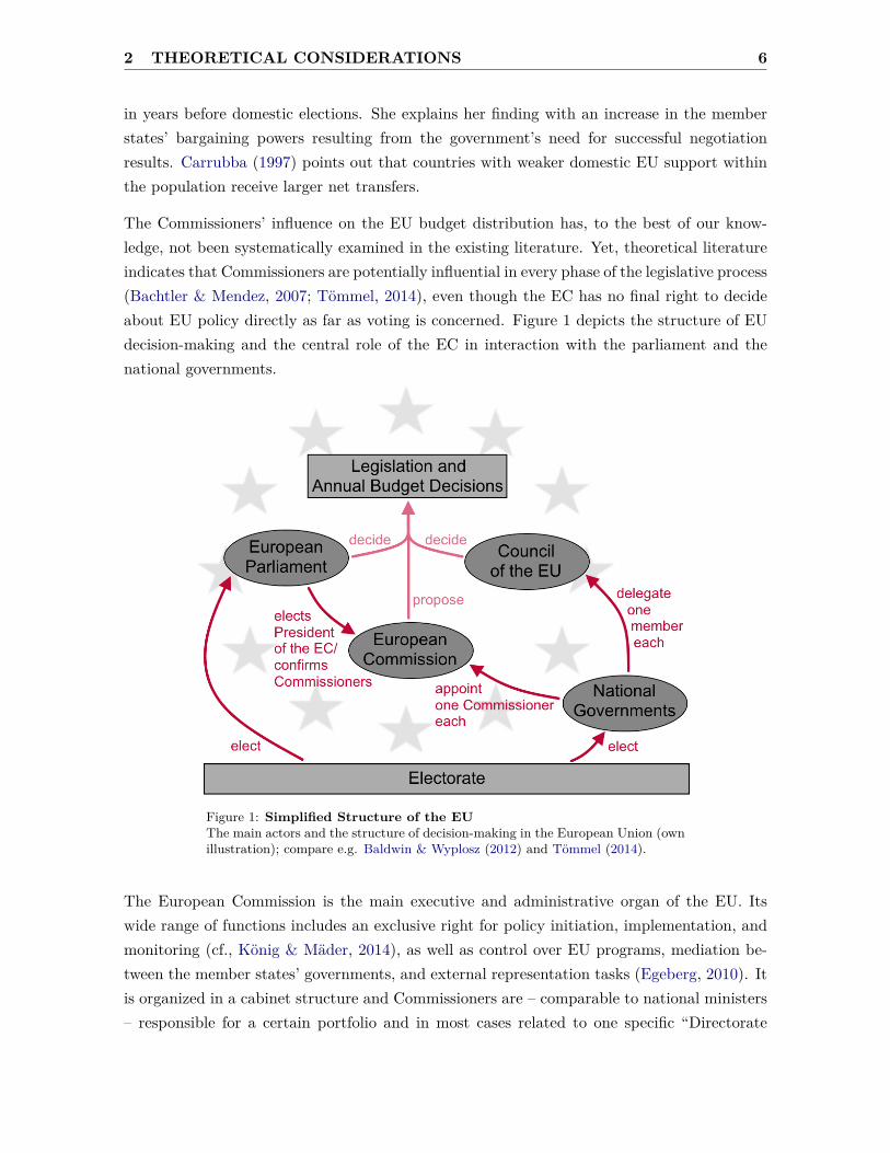
The Commissioners’ influence on the EU budget distribution has, to the best of our know-ledge, not been systematically examined in the existing literature. Yet, theoretical literatureindicates that Commissioners are potentially influential in every phase of the legislative process(Bachtler & Mendez, 2007; Tömmel, 2014), even though the EC has no final right to decideabout EU policy directly as far as voting is concerned. Figure 1 depicts the structure of EUdecision-making and the central role of the EC in interaction with the parliament and thenational governments.

Figure 1: Simplified Structure of the EUThe main actors and the structure of decision-making in the European Union (ownillustration); compare e.g. Baldwin & Wyplosz (2012) and Tömmel (2014).

The European Commission is the main executive and administrative organ of the EU. Itswide range of functions includes an exclusive right for policy initiation, implementation, andmonitoring (cf., König & Mäder, 2014), as well as control over EU programs, mediation be-tween the member states’ governments, and external representation tasks (Egeberg, 2010). Itis organized in a cabinet structure and Commissioners are – comparable to national ministers– responsible for a certain portfolio and in most cases related to one specific “Directorate

2 THEORETICAL CONSIDERATIONS 7

General” in the Commission’s administrative section.12 The appointment of the 27 Commis-sioners follows the principle: one country, one Commissioner. However, it is the Presidentof the EC who assigns the portfolios to the Commissioner candidates, which often results inunexpected portfolio allocations (Nugent, 2001). As outlined above, it is common that thespecific choices remain unclear until the day of the announcement, making the final allocationof the Commissioner positions close to random.

One can observe that, in contrast to past terms, member states nowadays increasingly delegatehigh ranked politicians (e.g., former national ministers) and members of the governing partyas Commissioners to Brussels (Egeberg, 2010; Döring, 2007). According to Wonka (2007),67.4% of the Commissioners, chosen by the member states from 1958 to 2006, came from thegoverning party and only 18.1% from the opposition. This suggests a principal-agent-structure(Vaubel, 2006; Wonka, 2007), where governments select reliable actors who are expectedto take national interests into account at the EU-level (Wonka, 2007). Although nationalgovernments have weaker means of exerting pressure and controlling the EC’s decisions in thepost-nomination phase (Vaubel, 2006), career-prospects (e.g., getting a leading position innational politics or elsewhere as a reward) and the option to be renominated for the lucrativejob are potential incentives to keep the country of origin’s (government’s) policy preferencesin mind (Döring, 2007; Vaubel et al., 2012).13 In line with these arguments, Vaubel et al.(2012, p.59) demonstrate how many Commissioners systematically plan their “life after theCommission”: In their sample, they find that 36% change to the private sector or lobby groupsand 43% return to national politics.

This political self-interest and the fact that candidates for the position are chosen by the na-tional governments suggests the possibility of potential conflicts of interest (Tömmel, 2014).14

On the one hand, all Commissioners owe their position to a system of proportional nationalrepresentation and a proposal of ‘their’ national government, but, on the other hand, they aresupposed to act independently and in the “general interest” (TEU). This conflict of interestscasts doubts on initial studies in political science which often described the Commission as aunitary technocratic actor, pursuing interests distinct from those of member states, and sup-ports authors like Wonka (2007), who more recently have rejected this assumption. He deemsit rather unlikely that the delegates – who are assumed to act like politicians – will collectivelyturn against the governments which once helped them take office. Thomson (2008) supportsthis notion by showing that Commissioners share the policy positions of the government oftheir country of origin.12 See also http://ec.europa.eu/commission/2014-2019_en (last accessed on May 4, 2015) for details on

the EC.13 In the context of two German cities, Potrafke (2013) provides another example of the relationship between

voter preferences and public spending in a principal-agent structure.14 In addition, current outside earnings could also create conflicts of interests, which we do not further consider

here as they are not systematically related to our research question. Focusing on members of the GermanBundestag, Arnold et al. (2014) find no clear relationship between outside earnings and parliamentary effort.

2 THEORETICAL CONSIDERATIONS 8

In fact, the nature of the EC has at all times raised the general suspicion of being an arena fornational interests. The Economist calls it “one of the better jokes in Brussels” that Commis-sioners are “completely independent” of their home countries.15 This notion is supported bysome anecdotal evidence. In 2007 and 2008, for example, the German Commissioner for Enter-prise and Industry, Günter Verheugen, repeatedly opposed a Commission proposal to reducenew car’s carbon dioxide emissions. This was widely perceived as support for the car indus-try, one of Germany’s most important economic sectors. Due to the opposition of Verheugen,the initial proposal by the Commissioner for Environment, Stavros Dimas, was weakened.Afterward, Dimas admitted that Verheugen “won against him” in the negotiations.16

Another example illustrates that nominated candidates do consider the promotion of nationalinterests part of their task. Before taking office in 2014, Vera Jourová, the current Commis-sioner for Justice, Consumers and Gender Equality, was asked about her aims as the newCzech EU Commissioner. She said that “[t]he European Commissioner must of course beimpartial, without regard to national interests. Beyond this, however, I would like to focuson coordinating the activities of Czech people in EU institutions to promote Czech nationalinterests – after my working hours, if you will.”17 These examples are in line with Egeberg(2006, p. 13) who remarks that “Commissioners as well as cabinet ministers have their ‘local’community back home which imposes certain expectations on them while in office.”

2.2 Identifying the Link Between Commissioners and Budget Items

Despite these studies and anecdotal evidence, it is not clear whether the above examplesconstitute exceptions or can be supported by empirical evidence. To be able to identify thisrelationship, it is of particular interest to consider the role, room to maneuver, and powerof the Commissioners in the legislative process. The Commission’s most relevant power isits monopolistic position as the agenda setter, characterized by an exclusive privilege tomake legislative, budgetary and program proposals in areas that fall under EU responsibility(Article 17, TEU). It can decide, on the whole, whether to take up policy propositions fromthe European Parliament (EP) and the Council or not (Bachtler & Mendez, 2007; Egeberg,2010): “The Council, the EP and member states may make suggestions to the Commissionand can call on the Commission to present new proposals, but it is the European Commissionthat actually drafts proposals” (Roozendaal & Hosli, 2012, p. 449). As a consequence, theCommission can exert influence by defining “the terms in which issues are discussed” (Hosli15 See The Economist, under http://www.economist.com/node/10171795 (last accessed on April 28, 2015).16 See Deutschlandfunk for the translated direct quote under http://www.deutschlandfunk.de/

autolobby-contra-klimaschutz.724.de.html?dram:article_id=98703 (last accessed on April 28, 2015)and EU Observer under https://euobserver.com/economic/25453 (last accessed on April 28, 2015).

17 For the direct quotation see Radio Praha under http://www.radio.cz/en/section/curraffrs/minister-vera-jourova-nominated-for-czech-eu-commissioner (last accessed on April 30, 2015), writ-ten July 21, 2014.

2 THEORETICAL CONSIDERATIONS 9

& Thomson, 2006, p. 397).18

In the run-up to the introduction of a new policy proposal, the Commissioners try to anticipateand consider possible supporting coalitions in the Council or EP. As “interface managers”(Tömmel, 2014, p. 152), it is their task to mediate between the legislative organs and to findcompromises with majority appeal. According to Hosli & Thomson (2006), the Commissionersare also continuously involved in discussions in the Council, and negotiations between the EPand the European Council. In addition to organizing majorities in the Council or EP, they alsoneed to win the support of their colleagues in the Commission. Hence, it is common practiceto do “package deals” (Tömmel, 2014, p. 152) in order to gain enough support for one’sproposal. Nevertheless, the intra-Commission decision-making process is a first control-levelthat might limit the ability of individual Commissioners to pursue their own agendas.

It seems plausible that Commissioners would use their informational advantages vis-à-vis theEP and the member states’ representatives in the Council (Döring, 2007; Hosli & Thomson,2006). These advantages are derived, for example, from the staff of their associated Direc-torate General or their consultations with external experts and acquisition of information frominterest groups in the early stages of the legislative process. As a consequence the Commission,which takes part in Council meetings, can try to forge political deals. Likewise, Commission-ers supposedly have informational advantages (albeit in a weaker form) in negotiations withother Commissioners (Thomson, 2008), when decisions in their field of activities are made.The decision-making process at these meetings and negotiations is opaque, however, and onlyscarcely documented; thus not allowing a systematic analysis of the relationship we are inter-ested in. To the best of our knowledge there exist no data that allows for the decompositionof individual Commissioners’ budgets so that they may be compared to the shares that eachmember country receives. The only data that are available in the necessary form relate to thevarious funds that the EU manages.

We focus on the EU Commissioner for Agriculture, the one case where an individual Com-missioner is solely responsible for payments from a specific fund, namely the European Agri-cultural Guidance and Guarantee Fund (EAGGF). This fund is the main pillar of the EU’sCommon Agricultural Policy and came into force in 1962. Up until now, the agricultural fundhas made up the greatest part of the EU’s overall expenditures (cf. Figure 2). In spite of twosubstantial reforms of the CAP in 1992 and 2003 that gradually shifted the EU’s agriculturalexpenditure from guaranteeing price support for agricultural products to individual direct18 Empirical evidence about the budgetary impact of such proposal powers is provided by Knight (2005). In-

vestigating the allocation of transportation projects in the U.S. in 1991 and 1998, he finds that congressionaldistricts which have a member on the transportation authorization committee and thus possess proposalpower, receive significantly more project spending than districts without a member on this committee.Bailer (2004) distinguishes between exogenous and endogenous power in the European Council. Exogenouspower includes economic strength and votes, while endogenous power is drawn from the proximity to theEC, which she relates to bargaining success.

2 THEORETICAL CONSIDERATIONS 10

payments for farms (decoupling) and rural development programs (Baldwin & Wyplosz, 2012;Fouilleux, 2010), the EAGGF was allocated consistently annually until 2007.

Figure 2: EU Budget StructureStructure of EU Expenditures, percentages of the total. Source: European Commis-sion, adapted from Butzen et al. (2006).

The CAP scheme is particularly well-suited to analyze the relationship between nationalbackground and budget allocation. It has a re-distributional nature and provides a classicexample of pork-barrel politics (Weingast et al., 1981), where each country supposedly aimsto acquire as many fund resources as possible. The CAP is a major and salient budgetaryitem in the overall budget. Hence, it is plausible that member states are interested in tryingto make use of “their” Commissioner as their popularity with the electorate at home candepend on their bargaining performance (Baldwin & Wyplosz, 2012; Schneider, 2013).19

A precise description of the annual CAP budget negotiations, which take place a year aheadof the actual budget year is provided by Fouilleux (2010, p. 344):

“CAP decision making usually begins with a proposal from the Commission [...]. The Agri-cultural Council meets monthly, more frequently than most of the EU Councils. One of these

19 We do not discuss the general welfare implications of this controversial redistributive policy here. A similarcase of how origin matters in politics documented at the within-country level is Stratmann & Baur (2002).In their analysis of the German Bundestag, they indicate that particularly first-past-the-post elected par-liamentarians seize opportunities for pork-barreling in an attempt to satisfy “their” electorate. Whetherand why more market-based approaches and less pork-barrel politics could lead to welfare improvements isbeyond the scope of this paper. Evidence that more reliance on market forces does not only lead to highergrowth rates but also relates to higher subjective well-being is, for example, presented by Gehring (2013).

2 THEORETICAL CONSIDERATIONS 11

meetings was usually set aside to discuss what was called the ‘price package’ for the followingyear, at which the member states decided on such issues as the level of guaranteed prices foreach product and the amount of quota by country” (Fouilleux, 2010, p. 344).20

Accordingly, the Agricultural Commissioner has multiple opportunities to influence budgetdistribution that go beyond gaining leverage through the EC’s budget proposals. Negotiating‘price packages’, their agenda setting position, and information advantages can be used toredirect funds.

The requirements for reliable identification of a causal relationship that we formulated aboveare only partly fulfilled by two of the other Commissioners: the Commissioner for the Budgetand the Commissioner for Regional Policy. Both are agenda setters in their respective realm,and responsible for EU funds. Regional policy is closely related to two structural funds: theEuropean Social Fund (ESF) and the European Regional Development Fund (ERDF). Theallocation of these funds is to a larger degree based on formal criteria, however, and theRegional Commissioner’s portfolio cannot be separated from the portfolios of other Commis-sioners as clearly.21 Schneider (2013, p. 466) explains that “since ERDF/ESF transfers areallocated on a project-level basis, states are more restricted in their annual negotiations tomove around already stipulated funds.”

The Budget Commissioner has the main responsibility for managing the budget negotiationswith the member states.22 However, he has more of an influence on the allocation of budgetstowards the individual budget items than on the distribution across member states, a respon-sibility which falls to the respective Commissioners or is decided by the whole Commission.Moreover, there is only limited room to maneuver in the annual budget negotiations due tothe constraints set by the long term multi-annual financial frameworks of the EU.23 Hence,we are convinced that examining the Commissioner for Agriculture provides the best optionto analyze the relationship between national background and Commissioners’ behavior. Itis a case where the Commissioners have the leeway to exert influence on an economicallysignificant decision where we can directly trace their decisions back to impacting a specificfund.20 Before the Lisbon-Treaty (2007), the European Parliament had little influence on budget decisions in the

field of CAP (see e.g. Crombez & Swinnen, 2011; Schneider, 2013).21 For example, one criterion is that “to be eligible for most of the ERDF/ESF resources, the per capita GDP

of the country has to fall below 75 percent of the average GDP in the EU” (Schneider, 2013). For furtherdetails on the funds and criteria of the ERDF and ESF fund see http://ec.europa.eu/regional_policy/en/funding/erdf/ and http://ec.europa.eu/social/main.jsp?langId=en&catId=1.

22 See the official homepage of the current Commissioner for official goals and responsibilities under http://ec.europa.eu/commission/2014-2019/georgieva_en (last accessed on April 30, 2015).

23 The multi-annual financial frameworks of the EU act as a severe constraint and are negotiated by the headsof governments for seven (previously five) years (Schneider, 2013). In the multiannual budget negotiations,the member states “outline EU spending by setting ceilings on expenditures for each budget categoryand on total expenditure” (Schneider, 2013, p. 465). Thus, relating annual budget data to the BudgetCommissioner might not provide enough variation to find a significant relationship.

3 DATA AND EMPIRICAL STRATEGY 12

3 Data and Empirical Strategy

3.1 Data

In the following we describe our variables of interest, and give a brief description of the relevantcontrol variables which are derived from Schneider (2013). Since the EU has undergone severalenlargement rounds (cf. Figure 3), the length of time that is covered depends on the respectivecountry’s timing of joining the EU. Bulgaria and Romania are not included as their one yearof membership from 2005-2006 does not allow for an estimation with country fixed-effects.We thus analyze a non-balanced panel for a maximum of 25 countries.

Figure 3: Dates of EU AccessionOwn graphic based on data provided by the European Commission.

As dependent variables, we are interested in the share of the EU budget that a particularcountry i receives at time t. Our main variable and the focus of our paper is the share ofthe EAGGF Budget that country i receives as a percentage of the total EU budget. Thebudget shares are derived from the annual reports of the European Court of Auditors andrange from 1979 to 2006. More recent information does not exist in a comprehensive way at

3 DATA AND EMPIRICAL STRATEGY 13

the moment.24

At present, there exists no comprehensive information for more recent years. We use the shareto be able to easily disentangle changes in the overall budget sizes from changes in relativeallocation. This way of measuring negotiation success is more robust when examining a totalbudget that changed over the course of time (Aksoy, 2010; Butzen et al., 2006).25 In additionto our focus on shares of the agricultural funds, we also test whether similar relationshipsexist for the overall budget and the regional and social funds.

Our variable of interest is the nationality of the respective Commissioner. We use multiplesources (see Appendix A) to gather the terms of the EU Commissioners for Agriculture overour sample period. We code a variable Commissioner that contains the share of a year thatcountry i provides this Commissioner (measured by months in office). Appendix A showsthe respective appointment and resignation dates of all Commissioners during our sampleperiod. With few exceptions, Commissioner has the nature of a binary variable (being 1,if the member state appoints the Commissioner in a certain year and 0 otherwise), becauseCommissions were usually replaced in January. The average tenure of office is three years.26

In addition, we also code variables Commissioner (B) and Commissioner (R) for the EUCommissioner for the Budget and the Commissioner for Regional Policy respectively.

For reasons of transparency and to allow comparability with the existing literature, we do notpropose our own set of control variables but rather adopt those in Schneider (2013). Her setof control variables is based on EU distribution principles (see, e.g., Bouvet & Dall’Erba 2010)as well as on previous findings in the literature. Note that our results holds when adding,for example, the changes or lags of this comprehensive set of control variables in addition.Appendix B provides the exact definitions and data sources. For our identification strategy24 The EAGGF was replaced by two follow-up funds in 2007 (http://ec.europa.eu/agriculture/index_

en.htm, last accessed on April 16, 2015). This is the main reason that our sample ends in 2007. As oneof these funds, the European Agricultural Fund for Rural Development (EAFRD) co-finances economicrural development programs of the member states (see http://ec.europa.eu/agriculture/cap-funding/funding-opportunities/index_en.htm, last accessed on April 22, 2015), it is more difficult to directlytrace its changes back to the actions of the Commissioner for Agriculture. It pursues goals similar tothose of the cohesion and regional funds and might thus be influenced by other Commissioners as well.Specifically, it mostly “co-finances the rural development programs of the Member States” (see http://ec.europa.eu/agriculture/cap-funding/funding-opportunities/index_en.htm, last accessed on May20, 2015). Compare Schneider (2013) for a short description of the data sources. The original reports areavailable from the authors on request.

25 Within the scope of this paper, we disregard contractual amendments which altered the distribution ofpower between the EU’s three main organs and changed the budgetary procedures. Crombez & Hix (2011)for instance argue that under qualified majority voting, it should be easier for the Commission to push itsinterest through by focusing on pivotal member states. The length of our sample, however, does not offerenough statistical power to make valid estimations for sub-periods. See Crombez (2000), Hosli & Thomson(2006), and Aksoy (2010) for consequences of the particular treaties, voting rules and the differences be-tween ‘consultation’ and ‘co-decision’ procedures and Heinemann (2003) for an investigation of the politicaleconomy of EU enlargement and treaty amendments.

26 Due to the fact that we focus on one out of all Commissioners, the treatment is relatively rare in comparisonto the counterfactual. Note that our results hold also with robust regression techniques which specificallytackle this concern.

3 DATA AND EMPIRICAL STRATEGY 14

it is most important that the controls condition on the most likely selection mechanisms.

Election Year (Binary) and Pre-election Year (Binary) are binary variables that account forthe years before and during domestic elections, which could relate to receiving “supportive”financial flows. Most importantly for us, we need to control for factors that could directlyrelate to receiving the Agricultural Commissioner: States with higher unemployment, a lowerdevelopment and higher dependence on agriculture might be more likely to provide the Com-missioner. We use data for Unemployment Rate, Per Capita GDP (EU=100) (100 equals theEU average) and Employment Agriculture (ln) (measuring the number of people employed inthe agricultural sector as a natural logarithm in millions) from Eurostat to account for selec-tion on these observables. We also use data are from Eurobarometer to measure DomesticEU Support (%). The EU might be more likely to grant a member state the AgriculturalCommissioner and increased budget shares if there is a high share of eurosceptics in theelectorate.

Table 1: Descriptive StatisticsN Mean SD Min Max

Agricultural Fund Share 383 3.89 3.90 0 17.49Overall Funds Share 383 5.98 5.21 0.02 20.84Regional/Social Funds Share 383 1.46 1.73 0 9.19Commissioner 383 0.07 0.26 0 1.00Commissioner (Binary) 383 0.08 0.27 0 1.00Commissioner (B) 383 0.06 0.24 0 1.00Commissioner (R) 383 0.07 0.26 0 1.00Time in Office 383 0.26 1.12 0 9.83Pre-election Year (Binary) 383 0.26 0.44 0 1.00Election Year (Binary) 383 0.27 0.45 0 1.00Employment Agriculture (ln) 383 5.60 1.58 0.99 8.01Number of EU Members 383 15.20 5.19 9.00 25.00Unemployment Rate 383 8.28 3.65 0.70 21.30Per Capita GDP (EU=100) 383 100.15 41.51 23.05 301.18New Member State (Binary) 383 0.22 0.42 0 1.00Voting Power Council (%) 383 7.24 4.67 0.90 17.86Domestic EU support (%) 383 45.78 22.81 -30.00 86.00Observations in sample from Table 2, column 4. N = number of observations,Mean = arithmetic mean, SD = standard deviation, Min = minimum value,Max = maximum value.

Bargaining power in the EU Council is quantified using the Shapley-Shubik index with thevariable Voting Power Council (%).27 New Member State (Binary) is a binary variable for allnew members until the next enlargement round of the EU, which is coded as 1 if a countryis a new member in this period and 0 otherwise. It accounts for the fact that new members27 For the exact calculation of the power indices see Bräuninger & König (2005).

3 DATA AND EMPIRICAL STRATEGY 15

receive lower budget shares initially because of their inferior administrative capacity and lessdeveloped bargaining experience in attracting a share of the funds (Plümper & Schneider,2007; Schneider, 2013). The variable Number of EU Members accounts for the enlargementsby controlling for the number of member states. Due to the enlargement rounds, the budgetshares that single member states receive decrease over time. These factors together shouldcapture the most important observable selection variables. Descriptive statistics are providedin Table 1.

3.2 Empirical Strategy

Our main estimation equation is

Yi,t = α+ βCi,t +X′i,tγ + ϑi + τt + εi,t,

where Yi,t is the budget share country i gets in year t, α is a constant, Ci,t is the variable forappointing the Commissioner for Agriculture, Xi,t represents the vector of control variables,ϑi are fixed-effects for country i, τt indicate time dummies and εi,t is an error term.

As mentioned above, we follow Schneider (2013) in the choice of control variables. We differ insome aspects from her specification, however. First, we add year dummies δt that account forunobservable year-specific variation that might bias the estimate of Ci,t. Second, Schneider(2013) uses panel-corrected standard errors (PCSE) to allow for panel-heteroscedasticity andcontemporaneously cross-sectionally correlated errors (Hoechle, 2007), and the Prais-Winstenestimator to allow for panel-specific first-order auto-correlation. The Feasible GeneralizedLeast Squares (FGLS) approach of PCSE offers potential efficiency gains, as it assumes onlyfirst-order auto-correlation of error terms within clusters. Though, it rests on the assumptionof correct specification of the error term structure and can be biased in the presence of cluster-specific fixed-effects.28

The fixed-effects (FE) within estimator with cluster-robust standard errors provides a moreconservative estimation that is less sensitive to misspecification. In cases of relatively smallcluster sizes, it is appropriate to use the within estimator standard errors for inference (seeDube and Lindo in Cameron & Miller, 2015). Our estimates are robust to using PCSE, as wewill demonstrate below, but we prefer the more conservative fixed-effects within estimator. Weuse two-way clustering where we cluster at the country and year level (Cameron et al., 2011).Because the dependent variable is a share out of all member states, there necessarily existscorrelation across observations at each point in time, which makes it important to cluster onyears as well. To estimate our regressions, we make use of the procedures developed by Baumet al. (2002) and Schaffer (2010).28 This happens because the standard errors of the fixed-effects are not consistently estimated. This would not

be problematic in settings where we are not specifically interested in the fixed-effects and their significancelevel. Here, however, the FGLS estimator is formed using these residuals (see Cameron & Miller, 2015).

4 RESULTS 16

4 Results

4.1 Main Results

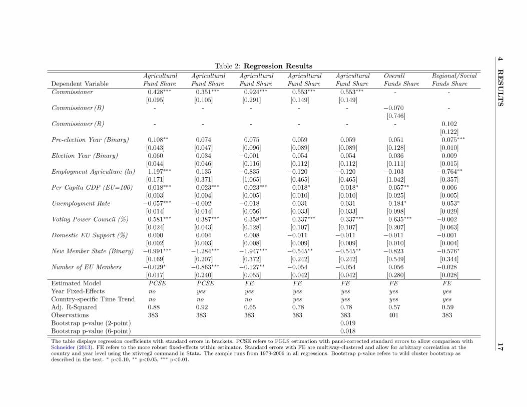
Table 2 shows the main results for the 1979-2006 period. For reasons of transparency andcomparability, the specification in column 1 uses PCSE as in Schneider (2013), and addsour Commissioner variable. The coefficient for Commissioner is positive and significant atthe 1%-level, and remains nearly unchanged when adding year fixed-effects in column 2. Incolumn 3, we replicate column 2, but use the more robust FE within estimator with standarderrors clustered at the country and year level. The coefficient for Commissioner is 0.924 andis significant at the 1%-level. Having the EU Commissioner for Agriculture is thus associatedwith an increase in the share of the overall EU budget obtained by the respective countryof approximately 1 percentage point. This change relates on average to an increase of about25% percent in the agricultural receipts for the home country and would translate to 850million EUR per year (for a fictive average sized country) based on the 2006 EU budget.

However, using general year dummies and country fixed-effects might not capture all unob-served variation over time. In their analysis of labor market regulation on manufacturingperformance in Indian states, for example, Besley & Burgess (2002) show that their mainfindings disappear after controlling for cluster-specific time trends. To resolve this matter, weadd country-specific time trends in addition to the year dummies to account for changes inthe share of agricultural funds within a country over the sample period. If sectoral changesin the industrial structure of individual countries lead to less money being allocated to thesecountries, this could bias our results if it coincides with providing the EU Commissioner.In fact, adding the trends leads to a decrease in the coefficient to 0.553 in column 5. Theestimate becomes more precise, however, and the standard error decreases, which again leadsto a rejection of the null-hypothesis of no relationship at the 1%-level. Hence, in this mostconservative specification, providing the Commissioner for Agriculture is still related to about0.5 percentage points higher fund shares. This is our preferred estimation which we use formost further tests.

Recently, MacKinnon & Webb (2014) suggested that inference, i.e., estimating the correctsignificance level of coefficients, might be affected by wildly different cluster sizes. Clustersizes hereby refer to the number of observations included in each cluster. In our sample, thecountries are contained with different numbers of years due to differences in their respectivetiming of EU access. We programmed a wild cluster bootstrap procedure based on the sug-gestions in the appendix of MacKinnon & Webb (2014), Cameron et al. (2008), and Cameron& Miller (2015).

4RESU

LTS

17

Table 2: Regression ResultsAgricultural Agricultural Agricultural Agricultural Agricultural Overall Regional/Social

Dependent Variable Fund Share Fund Share Fund Share Fund Share Fund Share Funds Share Funds ShareCommissioner 0.428∗∗∗ 0.351∗∗∗ 0.924∗∗∗ 0.553∗∗∗ 0.553∗∗∗ - -

[0.095] [0.105] [0.291] [0.149] [0.149]Commissioner (B) - - - - - −0.070 -

[0.746]Commissioner (R) - - - - - - 0.102

[0.122]Pre-election Year (Binary) 0.108∗∗ 0.074 0.075 0.059 0.059 0.051 0.075∗∗∗

[0.043] [0.047] [0.096] [0.089] [0.089] [0.128] [0.010]Election Year (Binary) 0.060 0.034 −0.001 0.054 0.054 0.036 0.009

[0.044] [0.046] [0.116] [0.112] [0.112] [0.111] [0.015]Employment Agriculture (ln) 1.197∗∗∗ 0.135 −0.835 −0.120 −0.120 −0.103 −0.764∗∗

[0.171] [0.371] [1.065] [0.465] [0.465] [1.042] [0.357]Per Capita GDP (EU=100) 0.018∗∗∗ 0.023∗∗∗ 0.023∗∗∗ 0.018∗ 0.018∗ 0.057∗∗ 0.006

[0.003] [0.004] [0.005] [0.010] [0.010] [0.025] [0.005]Unemployment Rate −0.057∗∗∗ −0.002 −0.018 0.031 0.031 0.184∗ 0.053∗

[0.014] [0.014] [0.056] [0.033] [0.033] [0.098] [0.029]Voting Power Council (%) 0.581∗∗∗ 0.387∗∗∗ 0.358∗∗∗ 0.337∗∗∗ 0.337∗∗∗ 0.635∗∗∗ −0.002

[0.024] [0.043] [0.128] [0.107] [0.107] [0.207] [0.063]Domestic EU Support (%) 0.000 0.004 0.008 −0.011 −0.011 −0.011 −0.001

[0.002] [0.003] [0.008] [0.009] [0.009] [0.010] [0.004]New Member State (Binary) −0.991∗∗∗ −1.284∗∗∗ −1.947∗∗∗ −0.545∗∗ −0.545∗∗ −0.823 −0.576∗

[0.169] [0.207] [0.372] [0.242] [0.242] [0.549] [0.344]Number of EU Members −0.029∗ −0.863∗∗∗ −0.127∗∗ −0.054 −0.054 0.056 −0.028

[0.017] [0.240] [0.055] [0.042] [0.042] [0.280] [0.028]Estimated Model PCSE PCSE FE FE FE FE FEYear Fixed-Effects no yes yes yes yes yes yesCountry-specific Time Trend no no no yes yes yes yesAdj. R-Squared 0.88 0.92 0.65 0.78 0.78 0.57 0.59Observations 383 383 383 383 383 401 383Bootstrap p-value (2-point) 0.019Bootstrap p-value (6-point) 0.018The table displays regression coefficients with standard errors in brackets. PCSE refers to FGLS estimation with panel-corrected standard errors to allow comparison withSchneider (2013). FE refers to the more robust fixed-effects within estimator. Standard errors with FE are multiway-clustered and allow for arbitrary correlation at thecountry and year level using the xtivreg2 command in Stata. The sample runs from 1979-2006 in all regressions. Bootstrap p-value refers to wild cluster bootstrap asdescribed in the text. ∗ p<0.10, ∗∗ p<0.05, ∗∗∗ p<0.01.

4 RESULTS 18

The program relies on a cluster bootstrap with asymptotic refinement, which is achievedby bootstrapping the pivotal Wald t-statistic. The Wald statistic is pivotal as it does notdepend on any unknown parameters in V [ε|X]. To generate the bootstrap dependent variableswe used the “Rademacher”-2-point distribution as well as the “Webb”-6-point distribution(Webb, 2013). The results with 10,000 repetitions can be seen in column 5. The p-value withthe Rademacher-distribution is 0.019, i.e., still corresponds to significance at the 5%-level.With the 6-point distribution, which, as Webb (2013) argues, further improves the reliabilityof statistical inference, the p-value becomes 0.018. Hence, we conclude that our baselineestimates of the relationship between providing the EU Commissioner for Agriculture andthe share received by the respective country of origin is robustly positive and significant. Itis also economically significant. The coefficient of 0.553 would translate into an increase inallocations of about 510 million EUR per year. This is a significant amount, particularly forsmaller member states. For example, Denmark’s overall EU fund receipts sum up to 1,455million EUR.

Other Commissioner positions might be used to redirect funds to their respective home coun-tries as well. As argued above, the other obvious candidates where such a relationship couldbe measured are the position of Budget Commissioner and Commissioner for Regional Policy.Yet, these relationships are less well-suited for a quantitative assessment than the Agricul-tural Commissioner as outlined above. We use our variables for Commissioner (B) andCommissioner (R) to test for a relationship with the overall budget share and the regionaland social fund’s share of the respective country of origin. As expected, we find no significantrelationship. Commissioner (B) relates to a coefficient of -0.070 and Commissioner (R) to0.102, and both are far from conventional significance levels. The most likely explanationis that either there is not enough leeway associated with these positions, the multi-annualfinancial framework restricts their room for maneuver, or there is too much noise in the datato be able to identify a significant relationship.29

With regard to the Agricultural Commissioner, it seems possible that the Commissioners’effectiveness in redirecting funds to their home country is enhanced with the time they stayin office. In practice, huge differences exist between Commissioners in terms of the degree ofpower they develop in office. Smith (2003) identifies several crucial factors, including theirpersonal network, or their ability to learn to use their latent power effectively. Suvarierol(2008) highlights that international contacts in Brussels are especially potent in this regard.Bases on this our hypothesis is the Commissioners’ personal networks (both within and outsideof the EC) improves with their time in office. This could improve their ability to pursuenational interests.

Table 3 shows the test of this hypothesis. First, column 2 demonstrates that our main resultsremain qualitatively unchanged when using a binary variable instead of the monthly shares of29 Placebo tests using Commissioner (B) and Commissioner (R) are provided in Table 4, Appendix D. As

expected, neither of them can explain a significant amount of the variation in Agricultural Fund Share.

4 RESULTS 19

Table 3: Regression ResultsAgricultural Agricultural Agricultural

Dependent Variable Fund Share Fund Share Fund ShareCommissioner 0.553∗∗∗ - -

[0.149]Commissioner (Binary) - 0.496∗∗∗ 0.320∗∗

[0.126] [0.143]Commissioner (Binary) - - 0.065× Time in Office [0.075]Controls yes yes yesObservations 383 383 383Adj. R-Squared 0.78 0.78 0.80The table displays regression coefficients with standard errors in brackets. Allcolumns use the fixed-effects within estimator. Standard errors are multiway-clustered and allow for arbitrary correlation at the country and year level usingthe xtivreg2 command in Stata. ‘Controls’ includes all control variables in Table 2,column 5. This includes country and year fixed-effects, as well as country-specifictime trends. ∗ p<0.10, ∗∗ p<0.05, ∗∗∗ p<0.01.

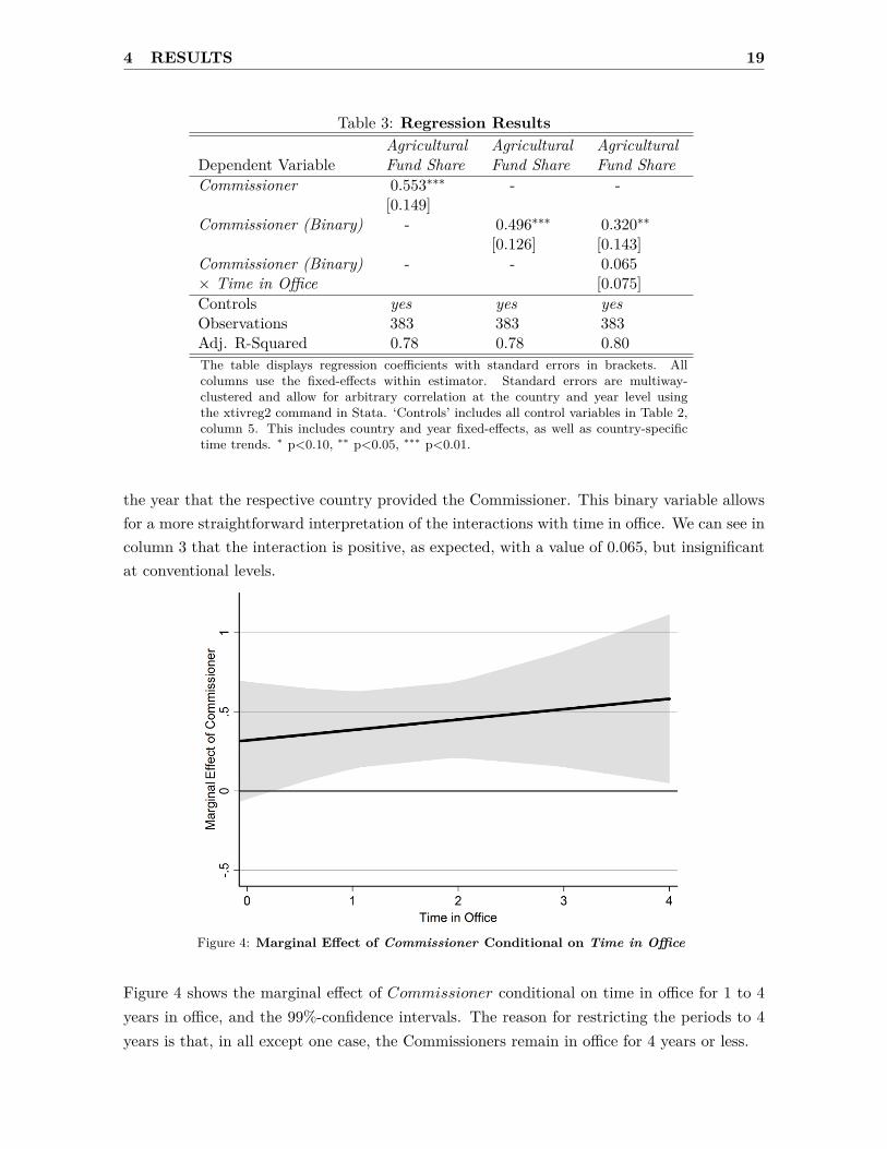
the year that the respective country provided the Commissioner. This binary variable allowsfor a more straightforward interpretation of the interactions with time in office. We can see incolumn 3 that the interaction is positive, as expected, with a value of 0.065, but insignificantat conventional levels.

Figure 4: Marginal Effect of Commissioner Conditional on Time in Office

Figure 4 shows the marginal effect of Commissioner conditional on time in office for 1 to 4years in office, and the 99%-confidence intervals. The reason for restricting the periods to 4years is that, in all except one case, the Commissioners remain in office for 4 years or less.

4 RESULTS 20

Although we remain cautious in interpreting the marginal effects due to the insignificance ofthe interaction term, they might tell us something about the mechanisms at work. It seemsplausible, that the Commissioner needs some time to adjust the budget due to his preferences.This is supported by the fact that the positive change becomes significant only after beingin office for at least one full year, and continues to increase over time. While using country-specific time trends alleviates endogeneity concerns, non-linear country-specific trends couldstill bias our estimations.

With the binary variable for Commissioner and year fixed-effects, our setting is exactly iden-tical to a difference-in-differences (DiD) estimation where providing the Commissioner inyear t is the treatment and all other countries form the respective control group. This com-parison is helpful as with DiD the crucial assumption that assures a causal interpretationof the estimated coefficient is common trends. In our multi-period setting, we can test thisassumption by examining whether different pre- or post-treatment trends exist for treatedand untreated countries which would indicate non-random selection. Including lead-variablesmakes it possible to inspect pre-treatment trends; including lag-variables allows for an assess-ment of differences after the treatment is stopped.

In this case, our theoretical considerations suggest that the Commissioners are able to affectbudget allocation in favor of their home country only once they are in office. A positive andsignificant lead-variable would thus cast doubts on the causal interpretation of our earlierresults as it would indicate different trends between treated and untreated countries. Sig-nificant lags are theoretically possible and not implausible; the Commissioners could eitherinstall staff that support their cause even after their dismissal or change internal processes orrules which take some time to reverse. Additionally even once agreed upon, implementing apolicy change usually takes some time.

We thus code two lead-variables, which take the value 1 only in the year (t−1) and two years(t − 2) before a country provides the Commissioner, and 0 otherwise. For post-trends, wecode four lag-variables that take the value 1 from one year after dismissal (t+ 1) to four yearsafter dismissal (t+ 4), and 0 otherwise.30

Table 4 depicts the results including different leads and lags. The specification is otherwiseidentical to our preferred specification above and includes the same controls. We estimateYi,t = α + βCi,t +

∑4ϕ=−2(βt+ϕCi,t+ϕ) + X

′i,tγ + ϑi + τt + εi,t with the binary indicator used

for Ci,t and with Xi,t including linear country-specific time trends (cf. the setting in Autor,2003). In column 1 it can be seen that both added lead-variables remain insignificant, whereasthe coefficient for Commissioner (t) increases marginally to 0.545 and remains significant30 We assign the 1 only for those cases where the country stopped providing the Commissioner in (t+1), i.e.,

where we can correctly identify post-treatment trends. We exclude the second to fourth year in office,where possibly the first to third lag could be coded as a 1. Otherwise, the variable would not capture apost-treatment effect the result be biased.

4 RESULTS 21

at the 1%-level. Column 2 adds lags instead of leads. Again, all the lag-variables are farfrom conventional significance levels, while Commissioner (t) increases to 0.692 and remainssignificant at the 1%-level. Finally, column 3 adds all leads and lags. Commissioner (t)increases further to 0.704 and remains significant at the 1%-level. All leads and lags areinsignificant, giving no indication of pre- and post-treatment trends, while Commissioner (t)remains significant throughout.

Table 4: Pre- and Post-Treatment TrendsAgricultural Agricultural Agricultural

Dependent Variable Fund Share Fund Share Fund ShareCommissioner (t-2) −0.050 - 0.053

[0.243] [0.194]Commissioner (t-1) −0.040 - 0.040

[0.378] [0.320]Commissioner 0.545∗∗∗ 0.692∗∗∗ 0.704∗∗∗

[0.149] [0.225] [0.218]Commissioner (t+1) - 0.732 0.740

[0.613] [0.611]Commissioner (t+2) - 0.477 0.484

[0.355] [0.347]Commissioner (t+3) - 0.039 0.048

[0.198] [0.177]Commissioner (t+4) - 0.093 0.099

[0.159] [0.127]Controls yes yes yesAdj. R-Squared 0.78 0.78 0.78Observations 383 383 383The table displays regression coefficients with standard errors in brackets. Allcolumns use the fixed-effects within estimator. Standard errors are multiway-clustered and allow for arbitrary correlation at the country and year level usingthe xtivreg2 command in Stata. ‘Controls’ includes all control variables in Table 2,column 5. This includes country and year fixed-effects, as well as country-specifictime trends. ∗ p<0.10, ∗∗ p<0.05, ∗∗∗ p<0.01. Table 6, Appendix D, demonstratesthat our results are also robust to including all lead- and lag-variables individually.

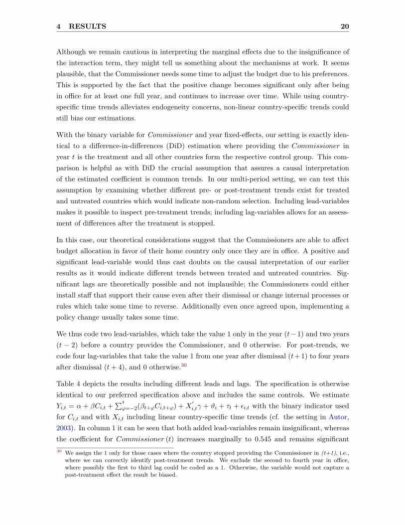
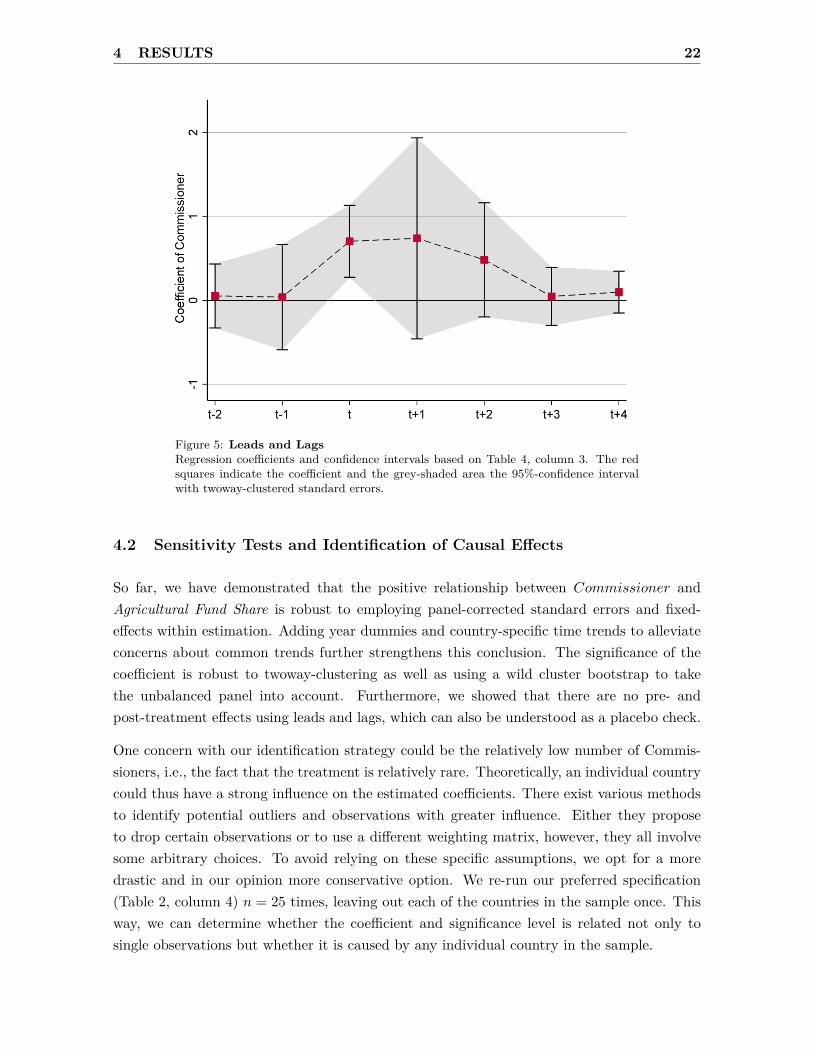
Figure 5 illustrates this graphically. The red squares indicate the coefficient and the grey-shaded area the 95%-confidence interval. It can be easily seen from the confidence-bandthat all leads and lags are far from being significantly different from 0. The graph showsthat the increase in fund shares occurs only during the time in office, remains positive butindistinguishable from 0 in the two years directly after the appointment of a new Commissionerfrom a different member state, and reverts back to 0 in (t + 3). This is a crucial result forthe causal interpretation of the identified relationship, as differences in trends were our mostserious concern. The next part will present further sensitivity tests and an assessment of therobustness of the coefficient to selection-on-unobservables.

4 RESULTS 22

Figure 5: Leads and LagsRegression coefficients and confidence intervals based on Table 4, column 3. The redsquares indicate the coefficient and the grey-shaded area the 95%-confidence intervalwith twoway-clustered standard errors.

4.2 Sensitivity Tests and Identification of Causal Effects

So far, we have demonstrated that the positive relationship between Commissioner andAgricultural Fund Share is robust to employing panel-corrected standard errors and fixed-effects within estimation. Adding year dummies and country-specific time trends to alleviateconcerns about common trends further strengthens this conclusion. The significance of thecoefficient is robust to twoway-clustering as well as using a wild cluster bootstrap to takethe unbalanced panel into account. Furthermore, we showed that there are no pre- andpost-treatment effects using leads and lags, which can also be understood as a placebo check.

One concern with our identification strategy could be the relatively low number of Commis-sioners, i.e., the fact that the treatment is relatively rare. Theoretically, an individual countrycould thus have a strong influence on the estimated coefficients. There exist various methodsto identify potential outliers and observations with greater influence. Either they proposeto drop certain observations or to use a different weighting matrix, however, they all involvesome arbitrary choices. To avoid relying on these specific assumptions, we opt for a moredrastic and in our opinion more conservative option. We re-run our preferred specification(Table 2, column 4) n = 25 times, leaving out each of the countries in the sample once. Thisway, we can determine whether the coefficient and significance level is related not only tosingle observations but whether it is caused by any individual country in the sample.

4 RESULTS 23

Table 5: Robustness to Outliers and Selection EffectsOmitted OmittedCountry Comm. Obs. Country Comm. Obs.Belgium 0.554∗∗∗ 355 Sweden 0.561∗∗∗ 371

[0.146] [0.150]Denmark 0.561∗∗∗ 355 United Kingdom 0.530∗∗∗ 356

[0.212] [0.159]Germany 0.557∗∗∗ 355 Cyprus 0.553∗∗∗ 380

[0.164] [0.149]Greece 0.530∗∗∗ 358 Malta 0.554∗∗∗ 380

[0.135] [0.149]Spain 0.544∗∗∗ 362 Czech Republic 0.553∗∗∗ 380

[0.135] [0.149]France 0.579∗∗∗ 355 Poland 0.553∗∗∗ 380

[0.203] [0.148]Ireland 0.689∗∗∗ 356 Slovenia 0.553∗∗∗ 380

[0.197] [0.149]Italy 0.496∗∗∗ 355 Slovakia 0.553∗∗∗ 380

[0.144] [0.149]Luxembourg 0.593∗∗∗ 355 Hungary 0.553∗∗∗ 380

[0.170] [0.149]Netherlands 0.414∗∗∗ 355 Estonia 0.553∗∗∗ 380

[0.104] [0.149]Autria 0.547∗∗∗ 371 Latvia 0.557∗∗∗ 380

[0.154] [0.149]Portugal 0.568∗∗∗ 362 Lithunia 0.553∗∗∗ 380

[0.139] [0.149]Finland 0.557∗∗∗ 371 Large Countries 0.451∗∗ 251

[0.151] [0.211]The table displays regression coefficients with standard errors in brackets. All columnsuse the fixed-effects within estimator. Standard errors are multiway-clustered and allowfor arbitrary correlation at the country and year level using the xtivreg2 command inStata. They include all control variables from Table 2, column 5. This includes countryand year fixed-effects, as well as country-specific time trends. Large Countries includeGermany, France, UK, Italy, Spain. ∗ p<0.10, ∗∗ p<0.05, ∗∗∗ p<0.01.

Table 5 shows that this does not seem to be the case. The left column indicates whichcountry was left out of the estimations, which, depending on the time of EU access, leads todifferent numbers of observations. We can see that the coefficient takes on values between0.414 (omitting the Netherlands) and 0.689 (omitting Ireland), but remains significant at the1%-level in all cases. Hence, the relative rareness of the treatment is not a serious problemfor identification. In addition, a sample without larger countries should exhibit a smallerselection bias as it excludes some countries that have a lower likelihood of being interested inthe Agricultural Commissioner post. When omitting the largest countries with more than 40million inhabitants, the relationship remains stable and significant at the 5%-level.

4 RESULTS 24

As a further robustness test, we also model non-linear selection on observables using anendogenous selection model. The model yields a larger coefficient for our main variable ofinterest, which remains significant at the 1%-level (see Appendix E for details). So far, we findno reason to doubt the interpretation of our coefficient as a causal effect of EU Commissioners’nationality on budget allocation behavior. Most importantly, we saw that while our treatmentis relatively rare, the coefficient estimate is surprisingly robust to the omission of each memberstate individually or all large countries jointly. In an admittingly somehow bold attempt, wenow test how move further we can extend our set of control variables.

First, not only the level of factors like the importance of the agricultural sector or EU supportin a member state, but also the change in these variables might affect the selection of theAgricultural Commissioner. When adding the changes to the levels, country and year fixed-effects, and linear time trends, our coefficient is barely affected and remains significant at the1%-level (see Table 7, Appendix D). Second, while the country specific linear trends controlfor important changes like the decline or rise of the agricultural sector in a member state,they might not fully capture these movement. Adding further polynomials captures furtherpotentially unobserved trend differences, but at the risk of capturing more and more of thevariation caused by the treatment, and inflating standard errors.31 In column 2-4 of Table 7,Appendix D, we first add quadratic, then cubic and finally quartic trends. As expected, thiscaptures part of the variation and slightly decreases the point estimates, but the coefficientsremain significant at the 5%-level. Third, the results are nearly identical when we combineall time trends and the changes in the control variables (see column 5, ibid.).

The fact that no form of selection-on-observables affects the estimations increases our confi-dence in interpretation of the results. To be able to speak about a causal interpretation, itwould still be desirable to assess to what degree selection-on-unobservables could still biasthe results. Thus, we finally compute the likelihood that our results can be explained byselection-on-unobservables. We first apply the methods developed in Altonji et al. (2005) toassess how much larger selection-bias based on unobserved factors would have to be comparedto observed factors to fully explain our results.

The strategy is to use selection-on-observables to assess the severity of potential selection biasfor the results. We compare two kinds of regressions: one with a limited set of controls (L =limited) to one with a full set of controls (F = full). Comparable to Nunn & Wantchekon(2011) we use two different sets for L and F. L1 contains country and year fixed-effects, L2

contains only country-fixed-effects. F1 comprises all variables from Table 2, column 3, and F2

adds the country-specific linear time trends to the former, i.e. responds to our most restrictive31 Mora & Reggio (2012) show that adding time trends and polynomials of further time trends is a more

flexible way to account for heterogenous unobserved variation. They also state that this procedure altersthe assumptions of the DiD framework. In addition, the correct average treatment effect would add thechange in the treated units captured by the time trend. We abstain from doing so here, and do not test theadjusted assumptions. Rather, we are interested in the stability of our point estimate and the significancelevel, which do not signal problematic divergences.

4 RESULTS 25

specification. We then calculate a “Selection ratio” (SR), which is the necessary ratio ofselection-on-unobservables to observables to fully explain our coefficients as | βF /(βF − βL) |.The denominator, i.e., the difference between the β coefficients indicates the degree to whichour estimate is affected by selection-on-observables. A small difference indicates little selectioneffects. βL in the nominator enters positively in the ratio, as we need stronger selection-on-unobservables to explain a larger coefficient. Altonji et al. (2005) provide the underlyingassumptions and Bellows & Miguel (2008) a formal derivation.

We have applied the relevant control variables as identified in Schneider (2013), withoutarbitrarily ‘picking’ our own set of control variables. These observed factors explain a largeshare of the variation in the dependent variable. So how likely is a bias due to unobservedtime-variant factors captured neither by the controls nor the country-specific time trends?The resulting ratios indicate that for L1,F1, selection-on-unobservables would have to be1.9 times as large as selection-on-observables to fully explain the positive relationship of thefund’s share with Commissioner for Agriculture. The respective ratios increase to nearly 5times for the L1,F2 and L2,F1 combinations. The smallest ratio is found when comparingL2,F2, but is still above one.

Table 6: Sensitivity to Selection-on-UnobservablesControls in the Controls in the SR = IdentifiedLimited Set Full Set βL βF | βF /(βL − βF )| β-Set

L1: Country-FE, F1: Country-FE, 0.43 0.92 1.88 [0.92; 1.52]Year-FE Year-FE,

Control Variables

L1: Country-FE, F2: Country-FE, 0.43 0.55 4.59 [0.55; 0.61]Year-FE Year-FE,

Control Variables,Timetrends

L2: Country-FE F1: Country-FE, 1.10 0.92 5.36 [0.85; 0.92]Year-FE,Control Variables,

L2: Country-FE F2: Country-FE, 1.10 0.55 1.02 [0.44; 0.55]Year-FE,Control Variables,Timetrends

The table reports regression coefficients for Commissioner and selection ratios (SR) based on the formuladepicted. Control variables include all country-specific and time-variant variables from prior regressions.A detailed defintion of the identified set is provided in the main text. The set is well identified if it doesnot include 0.

Oster (2013) provides an important formal extension of the intuition above. Due to spacerestrictions, we outline only the intuition and refer the reader to the paper for details. Again,we examine the change from βL to βF . As outlined above, we are less concerned by selection-

5 CONCLUDING REMARKS 26

on-unobservables if the coefficient moves away from 0 or shows only small changes towards0 when adding observables. However, Oster (2013) shows that small changes in the coeffi-cient only help in coming closer to a causal interpretation if the added variables also explainadditional variation in the dependent variable.

We need assumptions about the bounding value for Rmax, the maximum share of the variancethat can be systematically explained, and δ, the relationsip of selection-on-unobservableswith observables. She argues that Rmax ∈ [RF , 1] and δ ∈ [0, 1] are plausible boundaries.For simplicity, we use the most conservative setting with Rmax = 1 and δ = 1. We thencalculate the boundary of the set β∗ = βF − δ × (βL−βF )×(Rmax−RF )

(RF −RL) and the identified set∆s = [βF , β∗] ∀βF ≤ β∗ ∧∆s = [β∗, βF ] ∀βF > β∗.

Oster (2013) suggests that to assess a causal interpretation of the coefficient estimate, oneshould, for those cases where conditioning on observables moves β towards 0, examine whetherthe set includes 0, and whether its boundaries are within the confidence-interval of βF . Table 6shows that our identified set for the two cases where observables move us closer to 0 are [0.44;0.55] and [0.85; 0.92]; far from including 0. This is strong evidence that even with the mostconservative choice of the suggested boundaries, our full set is precisely estimated within theconfidence intervals and does not include 0. Overall, we find no plausible explanation thatholds as an argument against a causal interpretation of the identified relationship.

5 Concluding Remarks

The aim of this study was to examine whether and to what extent national backgroundinfluences budget allocation decisions in the European Union, which is in a continuous struggleabout the optimal level of integration. Proponents of more intense cooperation want toestablish a European state with strong central political authorities, while others pledge for alooser confederation or federal system with largely independent states with arguments relatingto heterogeneous preferences and common pool problems.32 At the same time, a growingnumber of radical parties want to largely reverse many of the prior integration steps. Againstthis background, examining the degree to which decisions of European Union actors are shapedby their respective national background is an important research question.32 Schneider (2014) argues that preference heterogeneity, bargaining dynamics, and the ability to find com-

promises for deeper cooperation on the EU level particularly depend on current domestic politics of the EUmembers and the number of member states. Preference heterogeneity seems to present the larger obstacleto cooperation, but adding new members does not in all circumstances amplify the problem. Janeba &Wilson (2011) model the optimal division of public good provision in a federal system with tax competitionand show that, while some goods should be centrally provided, complete centralization is never desirable forall public goods. Dreher et al. (2013) point at the role that differences in ‘soft’ private information betweenthe different layers in a federal system play in explaining the choice of sub-optimal decentralization levels.They also highlight that whether the upper or lower layers constitute the ‘principal’ in the principal-agentstructure determines how much information is shared and to what extent decision-making is in equilibriumdecentralized.

5 CONCLUDING REMARKS 27

Our focus was on the individual members of the European Commission, which is the mainexecutive organ of the EU. In contrast to other Commissioners where it is hard to traceand quantify their decisions, the Agricultural Commissioners fulfill all necessary requirementsto test the impact of national background. First, their roles actually give them enoughinfluence to be able to shift decisions in favor of their home countries. Second, the agriculturalbudget was and still is the main budgetary item in the overall EU budget, thus making therelationships under examination economically relevant. Third, we are able to calculate theshare of the budget that each member state receives for a sufficiently long time period byusing encoded EU budget lists and documents over the 1979-2006 period.

Our findings indicate that providing the Commissioner for Agriculture is related to increasesof about one percentage point in the share of the overall EU budget that the country of originreceives. This positive relationship is significant at the 1%-level. We remain cautious, butcannot find compelling reasons against a causal interpretation. Despite an extensive seriesof tests we find no plausible alternative explanations. These include testing the main as-sumption of no pre- or post-treatment trend differences, country specific time-trends, wildcluster bootstrap-procedures that are less sensitive to unequal cluster sizes, additional controlvariables, as well as omitting each member state individually and all large countries jointly.While omitted variables should always be a concern, we additionally computed that based onthe remaining variation in the dependent variable and the sensitivity to observables, alter-native explanations based on unobserved factors would have to assume an improbably highimpact of omitted variables (Oster, 2013). Hence, the results suggest that providing the EUCommissioner for Agriculture leads to increases in a country’s budget receipts.

This finding cannot necessarily be extrapolated to all other Commissioners and political actorsin the EU. Nevertheless, it presents clear and quantitatively relevant evidence that nationalbackground continues to matter in the EU. This does not rule out that Commissioners alsotake common European values and targets into account and are motivated by other motives ora European spirit. The evidence we provide is for the one case where the existing data make itpossible to identify a clear link to a precisely measurable outcome variable. Scientific cautionguides us to avoid premature conclusions. However, finding this robust and highly significantrelationship here changes the a priori assumptions about whether similar relationships alsoexists for other Commissioners, where a lack of data and transparency does not allow us toquantify them. To validate this finding with regard to other Commissioners, future researchshould, for example, aim to systematically collect new qualitative data.

Our findings should by no means be interpreted and used as evidence against the advance-ment of the EU, which is one of the most impressive and important political and economicprojects in the realm of international cooperation of the last half-century. Instead, we hope tobring awareness to the need to modify and adapt the political structures and the relationshipbetween member states and central authorities. This is upon the most pressing issues of the

5 CONCLUDING REMARKS 28

EU, but unfortunately does not receive the widespread public attention it deserves given theinfluence the Commission already has on the life of every European citizen.

The further development of the European Union should not repeat mistakes of the past andignore economic and social realities for the sake of avoiding political controversies and difficultbut much needed debates. One important direct policy implication is to take a realisticand cautious approach to international integration. There is now an impressive amount ofevidence that the national or regional background of politicians and bureaucratic actors stillshapes their decision-making when working at an international level. This should be takeninto account by designing mechanisms that minimize common pool problems and the abilityof individual actors and countries to over-proportionally exert their influence. The currentsystem that allocates one Commissioner per member state implicitly institutionalizes a systemof promoting national interests. Instead, the number of Commissioners should be based onefficiency concerns and selection should be decoupled from national origin, but rather bebased on the quality of the candidates. A renewed focus on the EU founding principle ofsubsidiarity would further help in alleviating concerns of citizens who perceive the EU asexcessively interfering in their lives. Finally, to regain lost confidence, the EU should ensuremore transparency about voting patterns and internal decisions, so that the public, mediaand science can provide the checks and balances necessary in a democratic system.

REFERENCES 29

References

Aksoy, Deniz. 2010. Who Gets What, When, and How Revisited: Voting and Proposal Powersin the Allocation of the EU Budget. European Union Politics, 11(2), 171–194. 3, 5, 13

Aksoy, Deniz. 2012. Institutional Arrangements and Logrolling: Evidence from the EuropeanUnion. American Journal of Political Science, 56(3), 538–552. 1

Alesina, Alberto, Angeloni, Ignazio, & Schuknecht, Ludger. 2005. What Does the EuropeanUnion Do? Public Choice, 123(3/4), 275–319. 5

Altonji, Joseph G., Elder, Todd E., & Taber, Christopher R. 2005. Selection on Observed andUnobserved Variables: Assessing the Effectiveness of Catholic Schools. Journal of PoliticalEconomy, 113(1), 151. 4, 24, 25

Arnold, Felix, Kauder, Björn, & Potrafke, Niklas. 2014. Outside Earnings, Absence, andActivity: Evidence from German Parliamentarians. European Journal of Political Economy,36, 147–157. 7

Autor, David H. 2003. Outsourcing at Will. Journal of Labor Economics, 21(1), 1–42. 4, 20

Bachtler, John, & Mendez, Carlos. 2007. Who Governs EU Cohesion Policy? Journal ofCommon Market Studies, 45(3), 535–564. 6, 8

Bailer, Stefanie. 2004. Bargaining Success in the European Union. European Union Politics,5(1), 99–123. 9

Baldwin, Richard E., & Wyplosz, Charles. 2012. The Economics of European Integration. 4.edn. London: McGraw-Hill Higher Education. 3, 6, 10

Barr, Jason, & Passarelli, Francesco. 2009. Who Has the Power in the EU? MathematicalSocial Sciences, 57(3), 339–366. 5

Baum, Christopher F., Schaffer, Mark E., & Stillman, Steven. 2002 (Apr.). Ivreg2: Stata Mod-ule for Extended Instrumental Variables/2SLS and GMM Estimation. Statistical SoftwareComponents, Boston College Department of Economics. 15

Bellows, John, & Miguel, Edward. 2008. War and Local Collective Action in Sierra Leone.Journal of Public Economics, 93(11), 1144–1157. 25

Besley, Timothy, & Burgess, Robin. 2002. The Political Economy of Government Responsive-ness. The Quarterly Journal of Economics, 117(4), 1415–1451. 16

Bouvet, Florence, & Dall’Erba, Sandy. 2010. European Regional Structural Funds: HowLarge Is the Influence of Politics on the Allocation Process? Journal of Common MarketStudies, 48(3), 501–528. 3, 13

Bräuninger, Thomas, & König, Thomas. 2005. Indices of Power IOP 2.0 [computer program].14

Brooks, Jonathan C., Cameron, A. Colin, & Carter, Colin A. 1998. Political Action CommitteeContributions and US Congressional Voting on Sugar Legislation. American Journal ofAgricultural Economics, 80(3), 441–454. 1

REFERENCES 30

Butzen, Paul, De Prest, Elianne, & Geeroms, Hans. 2006. Notable Trends in the EU Budget.Economic Review. Banque Nationale de Belgique. 10, 13

Cameron, A. Colin, & Miller, Douglas L. 2015. A Practitioners Guide to Cluster-RobustInference. Forthcoming in Journal of Human Resources, 221–236. 15, 16

Cameron, A. Colin, & Trivedi, Pravin K. 2005. Microeconometrics. Cambridge: CambridgeUniv. Press. 43

Cameron, A. Colin, Gelbach, Jonah B., & Miller, Douglas L. 2008. Bootstrap-Based Improve-ments for Inference with Clustered Errors. The Review of Economics and Statistics, 90(3),414–427. 16

Cameron, A. Colin, Gelbach, Jonah B., & Miller, Douglas L. 2011. Robust Inference withMultiway Clustering. Journal of Business & Economic Statistics, 29(2), 238–249. 15

Carnegie, Allison, Aronow, Peter M., & Marinov, Nikolay. 2014. Foreign Aid, Human Rightsand Democracy Promotion: Evidence from a Natural Experiment. Working Paper. 5

Carrubba, Clifford J. 1997. Net Financial Transfers in the European Union: Who Gets Whatand Why? The Journal of Politics, 59(2), 469–496. 5, 6

Crombez, Christophe. 2000. Institutional Reform and Co-Decision in the European Union.Constitutional Political Economy, 11(1), 41–57. 13

Crombez, Christophe, & Hix, Simon. 2011. Treaty Reform and the Commissioner’s Appoint-ment and Policy-Making Role in the European Union. European Union Politics, 12(3),291–314. 13

Crombez, Christophe, & Swinnen, Johan F. M. 2011. Political Institutions and Public Pol-icy: The Co-Decision Procedure in the European Union and the Reform of the CommonAgricultural Policy. LICOS Discussion Paper No. 286. 11

Döring, Holger. 2007. The Composition of the College of Commissioners. European UnionPolitics, 8(2), 207–228. 7, 9

Dreher, Axel, Sturm, Jan-Egbert, & Vreeland, James R. 2009a. Development Aid and Inter-national Politics. Journal of Development Economics, 88(1), 1–18. 5

Dreher, Axel, Lamla, Michael J., Lein, Sarah M., & Somogyi, Frank. 2009b. The Impact ofPolitical Leaders’ Profession and Education on Reforms. Journal of Comparative Economics,37(1), 169. 5

Dreher, Axel, Gehring, Kai, Kotsogiannis, Christos, & Marchesi, Silvia. 2013. InformationTransmission Within Federal Fiscal Architectures: Theory and Evidence. CESifo WorkingPaper Series No. 4400. 26

Dreher, Axel, Fuchs, Andreas, Hodler, Roland, Parks, Bradley, Raschky, Paul A., & Tierney,Michael J. 2015. Aid on Demand: African Leaders and the Geography of China’s ForeignAssistance. Working Paper. 3

REFERENCES 31

Egeberg, Morten. 2006. Executive Politics as Usual: Role Behaviour and Conflict Dimensionsin the College of European Commissioners. Journal of European Public Policy, 13(1), 1–15.8

Egeberg, Morten. 2010. The European Commission. In: Cini, Michelle, & Borragán, NievesPérez-Solárzano (eds), European Union Politics, 3. edn. Oxford: Oxford University Press.6, 7, 8

European Union. 2010. Consolidated Version of the Treaty on European Union. OfficialJournal of the European Union. 1

Fouilleux, Eve. 2010. The Common Agricultural Policy. In: Cini, Michelle, & Borragán,Nieves Pérez-Solárzano (eds), European Union Politics, 3. edn. Oxford: Oxford UniversityPress. 10, 11

Franck, Raphael, & Rainer, Ilia. 2012. Does the Leader’s Ethnicity Matter? Ethnic Favoritism,Education, and Health in Sub-Saharan Africa. American Political Science Review, 106(2),294. 5

Gawande, Kishore, & Hoekman, Bernard. 2006. Lobbying and Agricultural Trade Policy inthe United States. International Organization, 60(3), 527–561. 1

Gehring, Kai. 2013. Who Benefits from Economic Freedom? Unraveling the Effect of Eco-nomic Freedom on Subjective Well-Being. World Development, 50, 74–90. 10

Heinemann, Friedrich. 2003. The Political Economy of EU Enlargement and the Treaty ofNice. European Journal of Political Economy, 19(1), 17–31. 13

Hodler, Roland, & Raschky, Paul A. 2014. Regional Favoritism. The Quarterly Journal ofEconomics, 129(2), 995–1033. 3

Hoechle, Daniel. 2007. Robust Standard Errors for Panel Regressions with Cross-SectionalDependence. Stata Journal, 7(3), 281–312. 15

Hosli, Madeleine, & Thomson, Robert. 2006. Who Has Power in the EU? Journal of CommonMarket Studies, 44(2), 391–417. 8, 9, 13

Janeba, Eckhard, & Wilson, John Douglas. 2011. Optimal Fiscal Federalism in the Presenceof Tax Competition. Journal of Public Economics, 95(11), 1302–1311. 26

Jennes, Geert, & Persyn, Damiaan. 2015. The Effect of Political Representation on theGeographic Distribution of Income: Evidence Using Belgian Data. European Journal ofPolitical Economy, 37, 178–194. 3

Kauppi, Heikki, & Widgrén, Mika. 2004. What Determines EU Decision Making? Needs,Power or Both? Economic Policy, 19(39), 221–266. 5

Knight, Brian. 2005. Estimating the Value of Proposal Power. The American EconomicReview, 95(5), 1639–1652. 9

König, Thomas, & Mäder, Lars. 2014. The Strategic Nature of Compliance: An EmpiricalEvaluation of Law Implementation in the Central Monitoring System of the EuropeanUnion. American Journal of Political Science, 58(1), 246–263. 6

REFERENCES 32

Kuziemko, Ilyana, & Werker, Eric. 2006. How Much Is a Seat on the Security Council Worth?Journal of Political Economy, 114(5), 905–930. 5

MacKinnon, James G., & Webb, Matthew D. 2014. Wild Bootstrap Inference for WildlyDifferent Cluster Sizes. Queen’s Economics Department Working Paper No. 1314. 16

Maddala, Gangadharrao S. 1983. Limited-Dependent and Qualitative Variables in Economet-rics. 1. publ. edn. Cambridge: Cambridge Univ. Press. 43

Mazumder, Soumyajit, McNamara, Kathleen R., & Vreeland, James R. 2013. The Buck StopsHere: What Global Horse Trading Tells Us about the European Project. Working Paper. 5

Mora, Ricardo, & Reggio, Iliana. 2012. Treatment Effect Identification Using AlternativeParallel Assumptions. Universidad Carlos III de Madrid Economic Series Working Paper,48(12-33). 24

Napel, Stefan, & Widgrén, Mika. 2008. The European Commission. Public Choice, 137(1/2),21–41. 2, 3

Novosad, Paul, & Werker, Eric. 2014. Who Runs the International System? Power and theStaffing of the United Nations Secretariat. Power and the Staffing of the United NationsSecretariat (August 30, 2014). Harvard Business School BGIE Unit Working Paper. 2

Nugent, Neill. 2001. The European Commission. 1. publ. edn. The European Union Series.Houndmills: Palgrave. 2, 3, 7

Nunn, Nathan, & Wantchekon, Leonard. 2011. The Slave Trade and the Origins of Mistrustin Africa. The American Economic Review, 101(7), 3221–3252. 24

Olken, Benjamin A., & Jones, Benjamin F. 2005. Do Leaders Matter? The Quarterly Journalof Economics, 120(3), 835–864. 5

Olson, Mancur. 1965. The Logic of Collective Action. Harvard Economic Studies No. 124.Cambridge, Mass.: Harvard Univ. Press. 3

Oster, Emily F. 2013. Unobservable Selection and Coefficient Stability: Theory and Valida-tion. NBER Working Paper No. 19054. 4, 25, 26, 27

Plümper, Thomas, & Schneider, Christina J. 2007. Discriminatory European Union Mem-bership and the Redistribution of Enlargement Gains. The Journal of Conflict Resolution,51(4), 568–587. 15

Potrafke, Niklas. 2013. Evidence on the Political Principal-Agent Problem from Voting onPublic Finance for Concert Halls. Constitutional Political Economy, 24(3), 215–238. 7

Rodden, Jonathan. 2002. Strength in Numbers? European Union Politics, 3(2), 151–175. 5

Roozendaal, Peter, & Hosli, Madeleine O. 2012. Coalition Formation on Major Policy Dimen-sions. Public Choice, 153(3/4), 447–467. 8

Schaffer, Mark E. 2010. Xtivreg2: Stata Module to Perform Extended IV/2SLS,GMM and AC/HAC, LIML and k-class Regression for Panel Data Models.http://ideas.repec.org/c/boc/bocode/s456501.html. 15

REFERENCES 33

Schneider, Christina J. 2013. Globalizing Electoral Politics: Political Competence and Dis-tributional Bargaining in the European Union. World Politics, 65(3), 452–490. 3, 4, 5, 10,11, 12, 13, 15, 16, 25

Schneider, Christina J. 2014. Domestic Politics and the Widening-Deepening Trade-Off inthe European Union. Journal of European Public Policy, 21(5), 699–712. 26

Smith, Andy. 2003. Why European Commissioners Matter. Journal of Common MarketStudies, 41(1), 137–155. 3, 18

Stratmann, Thomas. 1992. The Effects of Logrolling on Congressional Voting. The AmericanEconomic Review, 1162–1176. 1

Stratmann, Thomas, & Baur, Martin. 2002. Plurality Rule, Proportional Representation, andthe German Bundestag: How Incentives to Pork-Barrel Differ across Electoral Systems.American Journal of Political Science, 46(3), 506–514. 10

Sturm, Jan-Egbert, & Wollmershäuser, Timo. 2008. The Stress of Having a Single MonetaryPolicy in Europe. KOF Working Paper No. 190. 2

Suvarierol, Semin. 2008. Beyond the Myth of Nationality: Analysing Networks Within theEuropean Commission. West European Politics, 31(4), 701–724. 18

Thomson, Robert. 2008. National Actors in International Organizations. Comparative Polit-ical Studies, 41(2), 169–192. 7, 9

Tömmel, Ingeborg. 2014. Das politische System der EU. 4. edn. Lehr- und Handbücher derPolitikwissenschaft. München: De Gruyter Oldenbourg. 6, 7, 9

Vaubel, Roland. 2006. Principal-Agent Problems in International Organizations. The Reviewof International Organizations, 1(2), 125–138. 7

Vaubel, Roland, Klingen, Bernhard, & Müller, David. 2012. There is Life After theCommission: An Empirical Analysis of Private Interest Representation by Former EU-Commissioners, 1981-2009. The Review of International Organizations, 7(1), 59–80. 2,7

Webb, Matthew D. 2013. Reworking Wild Bootstrap Based Inference for Clustered Errors.Queen’s Economics Department Working Paper No. 1315. 18

Weingast, Barry R., Shepsle, Kenneth A., & Johnsen, Christopher. 1981. The Political Econ-omy of Benefits and Costs: A Neoclassical Approach to Distributive Politics. Journal ofPolitical Economy, 89(4), 642–664. 10

Widgrén, Mika, & Kauppi, Heikki. 2007. Voting Rules and Budget Allocation in the EnlargedEU. European Journal of Political Economy, 23(3), 693–706. 5

Wonka, Arndt. 2007. Technocratic and Independent? The Appointment of European Com-missioners and its Policy Implications. Journal of European Public Policy, 14(2), 169–189.3, 7

6 APPENDIX 34

6 Appendix

6.1 Appendix A

Table 1: List of Agricultural CommissionersName Nation from toFinn Olav Gundelach1) Denmark January 6, 1977 January 13, 1981Poul Dalsager2) Denmark January 20, 1981 January 6, 1985Frans Andriessen3) Netherlands January 7, 1985 January 5, 1989Ray MacSharry4) Ireland January 6, 1989 January 5, 1993René Steichen5) Luxembourg January 6, 1993 January 24, 1995Franz Fischler6) Austria January 25, 1995 November 21, 2004Sandra Kalniete7) Latvia May 1, 2004 November 21, 2004Mariann Fischer Boel8) Denmark November 22, 2004 February 9, 2009

The exact dates were cross-verified using the following sources:1) http://www.spiegel.de/spiegel/print/d-14319885.html,

https://www.munzinger.de/search/document?index=mol-00&id=00000013522&type=text/html&query.key=szU1dQFW&template=/publikationen/personen/document.jsp&preview=,http://aei.pitt.edu/1535/

2) http://www.denstoredanske.dk/Dansk_Biografisk_Leksikon/Samfund,_jura_og_politik/Myndigheder_og_politisk_styre/Landbrugsminister/Poul_Dalsager,https://www.munzinger.de/search/document?index=mol-00&id=00000016216&type=text/html&query.key=rjym3Qji&template=/publikationen/personen/document.jsp&preview=,http://aei.pitt.edu/1535/

3) http://www.vieuws.eu/food-agriculture/frans-andriessen-former-commissioner-\penalty\z@for-agriculture-on-the-common-agricultural-policy-of-the-1980s/,https://www.munzinger.de/search/document?index=mol-00&id=00000017522&type=text/html&query.key=mQRbHaNY&template=/publikationen/personen/document.jsp&preview=,http://aei.pitt.edu/1535/

4) https://www.munzinger.de/search/document?index=mol-00&id=00000019420&type=text/html&query.key=5qx1jVy4&template=/publikationen/personen/document.jsp&preview=,http://aei.pitt.edu/1535/

5) https://www.munzinger.de/search/document?index=mol-00&id=00000020594&type=text/html&query.key=i6NxSr1K&template=/publikationen/personen/document.jsp&preview=,http://aei.pitt.edu/1535/

6) https://www.munzinger.de/search/document?index=mol-00&id=00000019235&type=text/html&query.key=KJFjpiKp&template=/publikationen/personen/document.jsp&preview=,http://aei.pitt.edu/1535/

7) https://www.munzinger.de/search/document?index=mol-00&id=00000024374&type=text/html&query.key=NF9rcU0k&template=/publikationen/personen/document.jsp&preview=,http://aei.pitt.edu/1535/

8) https://www.munzinger.de/search/document?index=mol-00&id=00000024988&type=text/html&query.key=LJmscBcr&template=/publikationen/personen/document.jsp&preview=

6 APPENDIX 35

Table 2: List of Regional CommissionersName Nation from toAntonio Giolitti1) Italy January 6, 1977 January 6, 1985Grigoris Varfis2) Greece January 7, 1985 December 31, 1985Alois Pfeiffer3) Germany January 1, 1986 August 1, 1987Peter Schmidhuber4) Germany September 22, 1987 January 5, 1989Bruce Millan5) United Kingdom January 6, 1989 January 24, 1995Monika Wulf-Mathies6) Germany January 25, 1995 September 17, 1999Michel Barnier7) France September 17, 1999 April 1, 2004Jacques Barrot8) France April 26, 2004 November 21, 2004Péter Balázs9) Hungary May 1, 2004 November 21, 2004Danuta Hübner10) Poland November 22, 2004 July 4, 2009

The exact dates were cross-verified using the following sources:1) https://www.munzinger.de/search/document?index=mol-00&id=00000010572&type=text/html&

query.key=AXXBQgGY&template=/publikationen/personen/document.jsp&preview=,http://aei.pitt.edu/1535/

2) http://aei.pitt.edu/1535/

3) https://www.munzinger.de/search/document?index=mol-00&id=00000017405&type=text/html&query.key=IFSCDeRs&template=/publikationen/personen/document.jsp&preview=,http://aei.pitt.edu/1535/

4) https://www.munzinger.de/search/document?index=mol-00&id=00000015616&type=text/html&query.key=icfj3I1o&template=/publikationen/personen/document.jsp&preview=,http://aei.pitt.edu/1535/

5) http://aei.pitt.edu/1535/

6) https://www.munzinger.de/search/document?index=mol-00&id=00000016843&type=text/html&query.key=eBQGuQmx&template=/publikationen/personen/document.jsp&preview=,http://aei.pitt.edu/1535/

7) https://www.munzinger.de/search/document?index=mol-00&id=00000023033&type=text/html&query.key=BL9HJPas&template=/publikationen/personen/document.jsp&preview=,http://aei.pitt.edu/1535/

8) https://www.munzinger.de/search/document?index=mol-00&id=00000014939&type=text/html&query.key=QDYGnRi0&template=/publikationen/personen/document.jsp&preview=,http://aei.pitt.edu/1535/

9) https://www.munzinger.de/search/document?index=mol-00&id=00000024894&type=text/html&query.key=2yKNVSDn&template=/publikationen/personen/document.jsp&preview=,http://aei.pitt.edu/1535/

10) https://www.munzinger.de/search/document?index=mol-00&id=00000024792&type=text/html&query.key=o09MaerS&template=/publikationen/personen/document.jsp&preview=

6 APPENDIX 36

Table 3: List of Budget CommissionersName Nation from toChristopher Tugendhat1) United Kingdom January 6, 1977 January 6, 1985Henning Christophersen2) Denmark January 7, 1985 January 5, 1989Peter Schmidhuber3) Germany January 6, 1989 January 24, 1995Erkki Liikanen4) Finland January 25, 1995 September 17, 1999Michaele Schreyer5) Germany September 17, 1999 November 22, 2004Marcos Kyprianou6) Cyprus May 1, 2004 November 22, 2004Dalia Grybauskaite7) Lithunia November 22, 2004 July 1, 2009

The exact dates were cross-verified using the following sources:1) https://www.munzinger.de/search/document?index=mol-00&id=00000014946&type=text/html&

query.key=WGH1rUUZ&template=/publikationen/personen/document.jsp&preview=,http://aei.pitt.edu/1535/

2) https://www.munzinger.de/search/document?index=mol-00&id=00000015397&type=text/html&query.key=6jbFAztz&template=/publikationen/personen/document.jsp&preview=,http://aei.pitt.edu/1535/

3) https://www.munzinger.de/search/document?index=mol-00&id=00000015616&type=text/html&query.key=eNQY73fw&template=/publikationen/personen/document.jsp&preview=,http://aei.pitt.edu/1535/

4) https://www.munzinger.de/search/document?index=mol-00&id=00000022864&type=text/html&query.key=Vl57hKR4&template=/publikationen/personen/document.jsp&preview=,http://aei.pitt.edu/1535/

5) https://www.munzinger.de/search/document?index=mol-00&id=00000019158&type=text/html&query.key=1J9aTjbF&template=/publikationen/personen/document.jsp&preview=,http://aei.pitt.edu/1535/

6) https://www.munzinger.de/search/document?index=mol-00&id=00000024888&type=text/html&query.key=mopXdm6j&template=/publikationen/personen/document.jsp&preview=,http://aei.pitt.edu/1535/

7) https://www.munzinger.de/search/document?index=mol-00&id=00000024892&type=text/html&query.key=WwKYz4qa&template=/publikationen/personen/document.jsp&preview=

EC collectively resigned on March 15, 1999 and remained in office executively until September 1999. Allweblinks last accessed on May 1, 2015.

6 APPENDIX 37

6.2 Appendix B

Description of Variables used:

Agricultural Fund Share1) Each member state’s annual agricultural fund (EAGGF) re-ceipts as a share of the overall annual EU budget (in %).

Overall Funds Share1) Each member state’s annual budget receipts as a share ofthe overall annual EU budget (in %).

Regional/Social Funds Share1) Each member state’s regional and social fund (ERDF/ESF)receipts as a share of the overall annual EU budget (in %).

Commissioner Proportion of the year in which a country appointed theAgricultural Commissioner (0 if country i did not appointthe Agricultural Commissioner in year t, 1 if the countryappointed the Agricultural Commissioner during the wholeyear). A month is counted, if the respective Commissionerwas in office for the major part of this month.

Commissioner (Binary) Dummy for appointing the Agricultural Commissioner (1 ifcountry i appoint the Agricultural Commissioner in in year tand if Commissioner is not 0, 0 otherwise).

Commissioner (B) Proportion of the year in which a country appointed theBudget Commissioner (0 if country i did not appoint theBudget Commissioner in year t, 1 if the country appointedthe Budget Commissioner during the whole year). A monthis counted, if the respective Commissioner was in office forthe major part of this month.

Commissioner (R) Proportion of the year in which a country appointed the Re-gional Commissioner (0 if country i did not appoint the Re-gional Commissioner in year t, 1 if the country appointed theRegional Commissioner during the whole year). A monthis counted, if the respective Commissioner was in office forthe major part of this month.

Time in Office Cumulated years in office as Agricultural Commissioner (1in the first year, 2 in the second year,...).

Commissioner (Binary)× Time in Office

Interaction of Commissioner (Binary) and Time in Office.

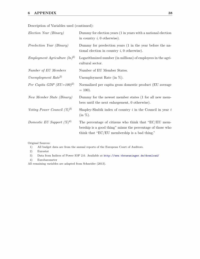
6 APPENDIX 38

Description of Variables used (continued):

Election Year (Binary) Dummy for election years (1 in years with a national electionin country i, 0 otherwise).

Preelection Year (Binary) Dummy for preelection years (1 in the year before the na-tional election in country i, 0 otherwise).

Employment Agriculture (ln)2) Logarithmized number (in millions) of employees in the agri-cultural sector.

Number of EU Members Number of EU Member States.

Unemployment Rate2) Unemployment Rate (in %).

Per Capita GDP (EU=100)2) Normalized per capita gross domestic product (EU average= 100).

New Member State (Binary) Dummy for the newest member states (1 for all new mem-bers until the next enlargement, 0 otherwise).

Voting Power Council (%)3) Shapley-Shubik index of country i in the Council in year t(in %).

Domestic EU Support (%)4) The percentage of citizens who think that “EC/EU mem-bership is a good thing” minus the percentage of those whothink that “EC/EU membership is a bad thing.”

Original Sources:1) All budget data are from the annual reports of the European Court of Auditors.2) Eurostat3) Data from Indices of Power IOP 2.0. Available at http://www.tbraeuninger.de/download/4) Eurobarometer

All remaining variables are adapted from Schneider (2013).

6 APPENDIX 39

6.3 Appendix C

Table 4: EU AccessionYear New Member States

∑1957 Belgium, France, Germany, Italy, Luxembourg, Netherlands 61973 Denmark, Ireland, United Kingdom 91981 Greece 101986 Portugal, Spain 121995 Austria, Finland, Sweden 152004 Estonia, Latvia, Lithunia, Malta, Poland, Slovakia, 25

Slovenia, Czech Republic, Hungary, Cyprus2007 Bulgaria, Romania 272012 Croatia 28The table lists the enlargement rounds of the EU. Column 3 shows the cumulativenumber of member states after the respective enlargement.Source: http://ec.europa.eu/enlargement/pdf/publication/factsheet_en.pdf

6 APPENDIX 40

6.4 Appendix D

Table 5: Robustness – Placebo TestsAgricultural AgriculturalFund Share Fund Share

Commissioner (R) 0.020 -[0.245]

Commissioner (B) - −0.422[0.268]

Controls yes yesAdj. R-Squared 0.78 0.78Number of Observations 383 383The table displays regression coefficients with standard errorsin brackets. All columns use the fixed-effects within estimator.Standard errors are multiway-clustered and allow for arbitrarycorrelation at the country and year level using the xtivreg2 com-mand in Stata. ‘Controls’ includes all control variables in Table2, column 5. This includes country and year fixed-effects, as wellas country-specific time trends. ∗ p<0.10, ∗∗ p<0.05, ∗∗∗ p<0.01.

6APPENDIX

41

Table 6: Individual Pre- and Post-Treatment TrendsAgricultural Agricultural Agricultural Agricultural Agricultural Agricultural AgriculturalFund Share Fund Share Fund Share Fund Share Fund Share Fund Share Fund Share

Comm/Agric (t-2) −0.254 - - - - - -[0.200]

Comm/Agric (t-1) - −0.158 - - - - -[0.410]

Comm/Agric - - 0.553∗∗∗ - - - -[0.149]

Comm/Agric (t+1) - - - 0.426 - - -[0.519]

Comm/Agric (t+2) - - - - 0.177 - -[0.175]

Comm/Agric (t+3) - - - - - −0.178 -[0.195]

Comm/Agric (t+4) - - - - - - −0.118[0.157]

Controls yes yes yes yes yes yes yesAdj. R-Squared 0.78 0.78 0.78 0.78 0.78 0.78 0.78Number of Observations 383 383 383 383 383 383 383The table displays regression coefficients with standard errors in brackets. All columns use the fixed-effects within estimator. Standard errors aremultiway-clustered and allow for arbitrary correlation at the country and year level using the xtivreg2 command in Stata. ‘Controls’ includes allcontrol variables in Table 2, column 5. This includes country and year fixed-effects, as well as country-specific time trends. ∗ p<0.10, ∗∗ p<0.05,∗∗∗ p<0.01.

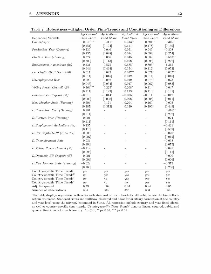
6 APPENDIX 42

Table 7: Robustness –HigherOrderTimeTrends andConditioning onDifferencesAgricultural Agricultural Agricultural Agricultural Agricultural

Dependent Variable Fund Share Fund Share Fund Share Fund Share Fund ShareComm/Agric 0.548∗∗∗ 0.411∗∗ 0.313∗∗ 0.381∗∗ 0.316∗∗

[0.151] [0.194] [0.151] [0.178] [0.159]Preelection Year (Dummy) −0.239 0.046 0.051 0.045 −0.308

[0.235] [0.088] [0.094] [0.098] [0.254]Election Year (Dummy) 0.377 0.066 0.045 0.089 0.563∗∗

[0.309] [0.113] [0.108] [0.098] [0.222]Employment Agriculture (ln) −0.131 0.575 0.685∗ 0.806∗ 1.315

[0.644] [0.464] [0.354] [0.412] [0.952]Per Capita GDP (EU=100) 0.017 0.022 0.027∗∗ 0.027∗ 0.037∗∗

[0.011] [0.015] [0.012] [0.014] [0.018]Unemployment Rate 0.029 −0.042 0.019 0.075 0.073

[0.043] [0.034] [0.047] [0.062] [0.083]Voting Power Council (%) 0.364∗∗∗ 0.225∗ 0.208∗ 0.11 0.047

[0.111] [0.123] [0.123] [0.113] [0.141]Domestic EU Support (%) −0.010 −0.014∗ −0.005 −0.011 −0.012

[0.009] [0.008] [0.008] [0.008] [0.011]New Member State (Dummy) −0.504∗ 0.171 −0.204 −0.169 −0.003

[0.287] [0.312] [0.320] [0.296] [0.449]D.Preelection Year (Dummy) 0.281 - - - 0.416∗∗

[0.211] [0.202]D.Election Year (Dummy) 0.001 - - - −0.024

[0.111] [0.111]D.Employment Agriculture (ln) 0.235 - - - −0.421

[0.416] [0.509]D.Per Capita GDP (EU=100) −0.003 - - - −0.020∗

[0.007] [0.012]D.Unemployment Rate 0.034 - - - −0.038

[0.100] [0.075]D.Voting Power Council (%) −0.119 - - - 0.025

[0.095] [0.111]D.Domestic EU Support (%) 0.001 - - - 0.000

[0.004] [0.006]D.New Member State (Dummy) −0.028 - - - −0.373

[0.166] [0.236]Country-specific Time Trends yes yes yes yes yesCountry-specific Time Trends2 no yes yes yes yesCountry-specific Time Trends3 no no yes yes yesCountry-specific Time Trends4 no no no yes yesAdj. R-Squared 0.79 0.82 0.84 0.84 0.85Number of Observations 364 383 383 383 364The table displays regression coefficients with standard errors in brackets. All columns use the fixed-effectswithin estimator. Standard errors are multiway-clustered and allow for arbitrary correlation at the countryand year level using the xtivreg2 command in Stata. All regression include country and year fixed-effects,as well as country-specific time trends. Country-specific Time Trendsi denotes linear, squared, cubic, andquartic time trends for each country. ∗ p<0.1, ∗∗ p<0.05, ∗∗∗ p<0.01.

6 APPENDIX 43

6.5 Appendix E

As we argue, selection among the smaller states seems to be largely random and unpredictable.To further remedy concerns about selection-on-unobservables that could bias our results up-or downwards, we further approach potential selection issues by using so-called endogenousbinary variable models (treatment effect models). There is no convincing instrument for ac-quiring a specific Commissioner that is excludable to our dependent variable. Instead, theapproach of these Heckit-models is similar to Heckman selection models: The selection prob-lem is solved by explicitly modeling selection instead of only proposing a supposedly exogenousinstrument. Treatment effect regressions differ from sample selection models as the binarytreatment variable is directly entered in the regression equation and the outcome variable isobserved for both the treated and the untreated subjects. The advantage of this potentialoutcome model is that it provides information about the effects of non-linear selection-bias.

Specifically, we model two equations. Our simplified regression equation is Yi,t = α+ βCi,t +X′i,tγ+ϑi+ τt+ εi,t, where Xi,t contains the controls and country-specific time trends and Ci,t

is the binary treatment indicator. Our probit selection-equation estimates the latent variableC∗i,t = Z

′i,tψ + ui,t with

Ci,t =

1 if C∗i,t > 0,

0 if C∗i,t ≤ 0

and Prob(Ci,t = 1 | Zi,t) = ∅(Z ′i,tψ), respectively,

Prob(Ci,t = 0 | Zi,t) = 1 − ∅(Z ′i,tψ). Zi,t is a vector of variables determining the selectionprocess. εi,t and ui,t are assumed to be bivariate normal with zero mean and covariance

matrix(σε ρ

ρ 1

), ρ 6= 0 reflects the assumed endogeneity of the treatment, and σ2

u = 1 for

identification.

This is a switching regression depending on whether C∗ > 0 or C∗ < 0, with separateforms for the outcome under treatment (Yi,t = β(Z ′i,tψ+ ui,t) +X

′i,tγ + εi,t) or non-treatment

(Yi,t = X′i,tγ + εi,t) regime. For a more detailed description see for example Cameron &

Trivedi (2005, sec. 16.7 and 25.3.4) and Maddala (1983). We conduct the estimation usingfull maximum likelihood under a normal distribution assumption.33

We do not claim that this approach resolves all potential selection-bias concerns, as it relies onassumptions about the correlation structure. Rather, we regard it as a further useful robust-ness check to assess the sensitivity of our results to changes in the econometric specificationand the direction of selection-bias. λ is the inverse Mills-ratio or non-selection hazard, and the33 Alternatively we can regard this model as a non-standard maximum-likelihood estimator. The likelihood

function LN (Θ) = f(y, X|Θ) = f(y|X, Θ)f(x|Θ) would generally require specifying the conditional densityof Y given X as well as the marginal density of X. It is standard to use only the conditional density f(y|X, Θ),and ignore f(X|Θ). This in essence assumes exogenous sampling and conditional independence. Treatmenteffect models drop this assumption, but instead assume a specific correlation structure of the error termsof the two equations to be estimated.

6 APPENDIX 44

parameter ρ indicates the correlation between the error terms εi.t and ui,t. We test the modelassumption with a likelihood ratio test of an independent probit and regression model versusthe treatment-effect likelihood, a test of ρ = 0 that is χ2 distributed. The Wald test-statisticrejects that ρ equals zero with a p-value of 0.004.

Table 8: Endogenous Selection ModelSelection Equation Treatment Equation

Dependent Variable Commissioner (Binary) Agricultural Fund SharePre-election Year (Binary) 1.994∗∗∗ [0.350] 0.024 [0.101]Election Year (Binary) 1.138∗∗∗ [0.270] 0.038 [0.103]Employment Agriculture (ln) 1.100 [1.135] −0.020 [0.493]Per Capita GDP (EU=100) 0.020 [0.013] 0.016∗ [0.009]Unemployment Rate 0.326∗∗∗ [0.123] 0.007 [0.031]Voting Power Council (%) −1.775∗∗∗ [0.601] 0.344∗∗∗ [0.108]Domestic EU Support (%) 0.069∗∗ [0.034] −0.014 [0.010]New Member State (Binary) 13.366∗∗∗ [1.810] −0.684∗∗∗ [0.234]Number of EU Members 2.059∗∗∗ [0.512] −0.053 [0.044]Commissioner (Binary) - 1.334∗∗∗ [0.352]Number of Cases 383 Rho −0.880Lamda −0.610 Prob > chi2(Rho=0) 0.004The table displays regression coefficients with standard errors in brackets. The model defines a treatedand untreated group based on Commissioner (Binary). Selection variables include all control variablesin Table 2, column 5. ∗ p<0.10, ∗∗ p<0.05, ∗∗∗ p<0.01.

The left part of Table 6 shows the results from the probit estimation of the likelihood toprovide the EU Commissioner for Agriculture for a certain year and country. We do notput too much weight on this equation, as it allows no clear causal interpretation, but givea brief summary. Factors significantly positively related to providing this Commissioner arePre-election Year (Binary) and Election Year (Binary), Unemployment Rate, Domestic EUSupport (%), and being a New Member State (Binary).34 Voting Power Council (%) is nega-tively related to Commissioner. Most interestingly for us is that Employment Agriculture (ln),i.e., a proxy for the importance of agriculture in the respective country, is not significantlyrelated to providing the Commissioner. Turning to the second-stage regression on AgriculturalFund Share in the right half of Table 6, the coefficient for Commissioner becomes larger at1.334 and remains significant at the 1%-level. Hence, taking selection into account with a fullmaximum-likelihood suggests that if there was selection bias before, it seems to have biasedCommissioner downwards rather than upwards. The larger effect would amount to about1,229 million EUR per year (based on the 2006 EU budget).

34 The Number of EU Members is also positively related but has no meaningful interpretation here.