transfer reinforcement learning with shared dynamics · pdf filetransfer reinforcement...
TRANSCRIPT
Transfer Reinforcement Learning with Shared Dynamics
Romain Laroche
Orange Labs at Châtillon, France
Maluuba at Montréal, Canada
Merwan Barlier
Orange Labs at Châtillon, France
Univ. Lille 1, UMR 9189 CRIStAL, France
AbstractThis article addresses a particular Transfer ReinforcementLearning (RL) problem: when dynamics do not change fromone task to another, and only the reward function does. Ourmethod relies on two ideas, the first one is that transition sam-ples obtained from a task can be reused to learn on any othertask: an immediate reward estimator is learnt in a supervisedfashion and for each sample, the reward entry is changed byits reward estimate. The second idea consists in adopting theoptimism in the face of uncertainty principle and to use upperbound reward estimates. Our method is tested on a navigationtask, under four Transfer RL experimental settings: with aknown reward function, with strong and weak expert knowl-edge on the reward function, and with a completely unknownreward function. It is also evaluated in a Multi-Task RL ex-periment and compared with the state-of-the-art algorithms.Results reveal that this method constitutes a major improve-ment for transfer/multi-task problems that share dynamics.
1 IntroductionReinforcement Learning (RL, (Sutton and Barto 1998)) isa framework for optimising an agent behaviour in an envi-ronment. It is generally formalised as a Markov DecisionProcess (MDP): hS,A, R, P, �i where S the state space, andA the action space are known by the agent. P : S ⇥A ! S ,the Markovian transition stochastic function, defines the un-known dynamics of the environment. R : S ! R, the im-mediate reward stochastic function, defines the goal(s)1. Insome settings such as dialogue systems (Laroche et al. 2009;Lemon and Pietquin 2012) or board games (Tesauro 1995;Silver et al. 2016), R can be inferred directly from the state bythe agent, and in some others such as in robotics and in Atarigames (Mnih et al. 2013; 2015), R is generally unknown.Finally, � 2 [0, 1) the discount factor is a parameter given tothe RL optimisation algorithm favouring short-term rewards.As a consequence, the RL problem consists in (directly orindirectly) discovering P , sometimes R, and planning.
Even when R is unknown, R is often simpler to learnthan P : its definition is less combinatorial, R is generallyCopyright c� 2016, Association for the Advancement of ArtificialIntelligence (www.aaai.org). All rights reserved.
1In this article, reward functions are defined on state represen-tation S, but all the results can be straightforwardly transposed torewards received after performing an action in a given state, i.e. toreward function defined on S ⇥A.
sparse, only a mean estimation is required, R tends to beless stochastic than P , and finally it is frequently possiblefor the designer to inject expert knowledge: for instance, anadequate state space representation for R, the uniqueness ofthe state with a positive reward, its determinism or stochasticproperty, and/or the existence of R bounds: R
min
and R
max
.Discovering (directly or indirectly) P and R requires col-
lecting trajectories. In real world problems, trajectory col-lection is resource consuming (time, money), and TransferLearning for RL (Taylor and Stone 2009; Lazaric 2012),through reuse of knowledge acquired from similar tasks, hasproven useful in many RL domains: Atari games (Romoff,Bengio, and Pineau 2016), robotics (Taylor, Stone, and Liu2007), or dialogue (Genevay and Laroche 2016). In this ar-ticle, we address the problem of Transfer ReinforcementLearning with Shared Dynamics (TRLSD), i.e. the transferproblem when P is constant over tasks ⌧ 2 T , which thusonly differ from each other by their reward functions R
⌧
. Weinclude the Multi-Task RL variation of this problem underthis denomination, i.e. when learning is made in parallel onseveral tasks. This family of problems may be encounteredfor instance in robotics, where the robot agent has to under-stand the complex shared environment dynamics in order toperform high level tasks that rely on this understanding.
In this article, we advocate that experience gathered ona task can be indirectly and directly reused on another taskand that transfer can be made at the transition sample level.Additionally, the optimism in the face of uncertainty prin-ciple allows to guide the exploration efficiently on a newtask, thanks to the dynamics knowledge transferred from theother tasks. The combination of those two principles allowsus to define a general algorithm for TRLSD, on a continu-ous state space, enabling the injection of task related expertknowledge.
Section 2 offers an overview of the known studies relatedto TRLSD, and introduces the principles of transition samplesharing between tasks. Then, Section 3 recalls the optimism
in the face of uncertainty principle, explains how to apply it toour setting, and explores different ways of computing this op-timism, inspired from the UCRL algorithm. Finally, Section4 presents various experiments illustrating and demonstrat-ing the functioning of our algorithms in Transfer RL andMulti-Task RL experiments. The experimental results demon-strate the significant improvement brought by our approach,
in comparison with the state-of-the-art algorithms in TRLSD.
2 Background and PrincipleTo the authors knowledge at the time they write this article,only two recent works were dedicated to TRLSD. First, (Bar-reto et al. 2016) present the framework as a kind of hierarchi-cal reinforcement learning, where composite and compound-able subtasks are discovered by generalisation over tasks. Inorder to do so, tasks share the successor features2 of theirpolicies, which are invariant from one task to another. Theirdecomposition of the reward function from the dynamics isunfortunately restricted to policies characterising the succes-sor features. Additionally, the theoretical analysis dependson R
⌧
similarities, which is not an assumption that is madein this article. Second, (Borsa, Graepel, and Shawe-Taylor2016) address the same problem in a Multi-Task RL settingby sharing the value-function representation: they build a tran-sition sample set for all tasks and apply generalised versionsof Fitted-Q iteration (Ernst, Geurts, and Wehenkel 2005)and Fitted Policy Iteration (Antos, Szepesvári, and Munos2007) learning on those transitions as a whole. The gener-alisation amongst tasks occurs in the regularisation used inthe supervised learning step of Fitted-Q iteration (and policyiteration/evaluation).
Instead of sharing successor features or value-function rep-resentations, we argue that transition samples can be sharedacross tasks. A transition sample (or sample in short) is classi-cally defined as a 4-tuple ⇠ = hs, a, r, s0i, where s is the stateat the beginning of the transition, a is the action performed, ris the reward immediately received, and s
0 is the state reachedat the end of the transition. For Transfer and Multi-Task RL,it is enhanced with task ⌧ to keep in memory which task gen-erated the sample: ⇠
⌧
= h⌧, s, a, r, s0i. Formulated in anotherway, s is drawn according to a distribution depending on thebehavioural policy ⇡⌧ , a according to the behavioural policy⇡
⌧
(s), r according to the reward function R
⌧
(s) of task ⌧and s
0 according to the shared dynamics P (s, a).As a consequence, with a transition sample set for all
tasks ⌅ =
S⌧2T ⌅⌧
, one can independently learn ˆ
P , anestimate of P , in a supervised learning way. In the samemanner, with the sample set constituted exclusively of task ⌧transitions ⌅
⌧
, one can independently learn ˆ
R
⌧
, an estimateof the reward function expected value E[R
⌧
], in a supervisedlearning way. This is what model-based RL does (Mooreand Atkeson 1993; Brafman and Tennenholtz 2002; Kearnsand Singh 2002). In other words, if transition sample ⇠
⌧
wasgenerated on task ⌧ , and if task ⌧ 0 shares the dynamics P
with ⌧ , then ⇠⌧
can be used for learning the dynamics modelof task ⌧ 0. The adaptation to non-stationary reward functionshas been an argument in favour of model-based RL for twentyyears. In particular, (Atkeson and Santamaria 1997) appliesit successfully on a task transfer with shared dynamics andsimilar reward functions on the inverted pendulum problem.
Nevertheless, this approach has never been theorised norapplied to Transfer or Multi-Task RL. We also advocate that
2A successor feature, a.k.a. feature expectation in (Ng and Rus-sell 2000), is a vector summarising the dynamics of the Markovchain induced by a fixed policy in a given environment.
learning the dynamics model P is not necessary and thatefficient policies can be learnt in a direct fashion: given atarget task ⌧ , any transition sample ⇠
⌧
0= h⌧ 0, s, a, r, s0i
from any other task ⌧
0 6= ⌧ can be projected on task⌧ , just by modifying the immediate reward r with ˆ
R
⌧
(s),the estimate of the reward function expected value E[R
⌧
]:
R̂⌧(⇠
⌧
0) = h⌧, s, a, ˆR
⌧
(s), s
0i. The approach consists thusin translating the transition sample set ⌅ into ˆ
R
⌧
estimate:
R̂⌧(⌅) = {
R̂⌧(⇠
⌧
0)}
⇠⌧02⌅, and then in using any off-policy RL algorithm to learn policy ⇡
⌧
on R̂⌧
(⌅). Theoff-policy characteristic is critical in order to remove thebias originated from the behavioural policies ⇡⌧ controllingthe transition sample set ⌅ generation. In our experiments,we will use Fitted-Q Iteration (Ernst, Geurts, and Wehenkel2005). The following subsection recalls the basics.
Fitted-Q IterationThe goal for any reinforcement learning algorithm is to finda policy ⇡⇤ which yields optimal expected returns, i.e. whichmaximises the following Q-function:
Q
⇤(s
t
, a
t
) = Q
⇡
⇤(s
t
, a
t
) = argmax
⇡
E⇡
st,at
2
4X
t
0�0
�
t
0r
t
0+t
3
5.
The optimal Q-function Q
⇤ is known to verify Bellman’sequation:
Q
⇤(s, a) = E
hR(s, a, s
0) + �max
a
0Q
⇤(s
0, a
0)
i(1)
, Q
⇤= T
⇤Q
⇤. (2)
The optimal Q-function is thus the fixed point of Bell-man’s operator T
⇤. Since � < 1, it is a contraction, andBanach’s theorem ensures its uniqueness. Hence, the optimalQ-function can be obtained by iteratively applying Bellman’soperator to some initial Q-function. This procedure is calledValue Iteration.
When the state space is continuous (or very large) it is im-possible to use Value-Iteration as such. The Q-function mustbe parametrised. A popular choice is the linear parametrisa-tion of the Q-function (Sutton and Barto 1998; Chandramo-han, Geist, and Pietquin 2010):
Q(s, a) = ✓
>�(s, a), (3)
where �(s, a) = {1a=a
0�(s)}
a
02A is the feature vector forlinear state representation, 1
a=a
0 is the indicator function,�(s) are the features of state s, and ✓ = {✓
a
}a2A is the
parameter vector that has to be learnt. Each element of ✓a
represents the influence of the corresponding feature in theQ-function.
The inference problem can be solved by alternately apply-ing Bellman’s operator and projecting the result back ontothe space of linear functions, and iterating these two stepsuntil convergence.
✓
(i+1)= (X
>X)
�1X
>y
(i), (4)
where, for a transition sample set ⌅ = {⇠j
}j2J1,|⌅|K =
{hsj
, a
j
, s
0j
, r
j
i}j2J1,|⌅|K, X is the observation matrix, which
lines are the sj
feature vectors: (X)
j
= �(s
j
, a
j
), and y
(i) isa vector with elements (y(i))
j
= r
j
+ �max
a
0✓
(i)�(s
0j
, a
0).
Data: ⌅: transition sample set on various tasksData: ⌅
⌧
✓ ⌅: transition sample set on task ⌧Learn on ⌅
⌧
an immediate reward proxy: ˜
R
⌧
;Cast sample set ⌅ on task ⌧ :
R̃⌧(⌅);
Learn on R̃⌧
(⌅) a policy for task ⌧ : ⇡⌧
;Algorithm 1: Transition reuse algorithm
3 Optimism in the Face of UncertaintyThe batch learning presented in last section proves to beinefficient in online learning: using an estimate ˆ
R
⌧
of R⌧
isinefficient in early stages, when only a few samples have beencollected on task ⌧ and reward has never been observed inmost states, because the algorithm cannot decide if it shouldexploit or explore further. We generalise our approach to areward proxy ˜
R
⌧
in Algorithm 1.In order to guide the exploration, we adopt the well-known
optimism in the face of uncertainty heuristic, which can befound in Prioritized Sweeping (Moore and Atkeson 1993),R-MAX (Brafman and Tennenholtz 2002), UCRL (Auer andOrtner 2007), and VIME (Houthooft et al. 2016). In the op-timistic view, ˜
R
⌧
is the most favourable plausible rewardfunction. Only UCRL and VIME use an implicit represen-tation of the exploration mechanism that is embedded intothe transition and the reward functions. The way UCRL sepa-rates the dynamics uncertainty from the immediate rewardsuncertainty makes it more convenient to implement and thefollowing of the article is developed with UCRL solution, butany other optimism-based algorithm could have been consid-ered in its place. (Lopes et al. 2012) and (Osband, Roy, andWen 2016) are also proposing interesting alternative optionsfor guiding the exploration.
Upper Confidence Reinforcement LearningUCRL algorithm keeps track of statistics for rewards andtransitions: the number of times N(s, a) action a in state s
has been performed, the average immediate reward r̂(s) instate s, and the observed probability p̂(s, a, s
0) of reaching
state s
0 after performing action a in state s. Those statisticsare only an estimate of their true values. However, confidenceintervals may be used to define a set M of plausible MDPsin which the true MDP belongs with high probability. As saidin last paragraph, UCRL adopts the optimism in the face of
uncertainty principle over M and follows one of the policiesthat maximise the expected return in the most favourableMDP(s) in M. The main idea behind the optimism explo-ration is the fact that mistakes will be eventually observedand knowledge of not doing it again will be acquired andrealised through a narrowing of the confidence interval.
One UCRL practical problem is the need for searchingthe optimal policy inside M (Szepesvári 2010), which iscomplex and computer time consuming. In our case, we canhowever consider that ˆ
P is precise enough in comparisonwith ˆ
R
⌧
and that dynamics uncertainty should not guide theexploration. Therefore, the optimal policy on M is necessar-ily the optimal policy of the MDP with the highest rewardfunction inside the confidence bounds, i.e.
˜
R
⌧
(s) defined by
the following equation:˜
R
⌧
(s) =
ˆ
R
⌧
(s) + CI
⌧
(s), (5)where CI
⌧
(s) is the confidence interval of reward estimateˆ
R
⌧
in state s. Afterwards, the optimal policy can be directlylearnt on data
R̃⌧(⌅) with Fitted-Q Iteration.
Another UCRL limitation is that it does not accommodatecontinuous state representations. If a continuous state rep-resentation �(S) = Rd needs to be used for estimating ˜
R
⌧
,UCCRL (Ortner and Ryabko 2012) or UCCRL-KD (Laksh-manan, Ortner, and Ryabko 2015) have been considered. But,they suffer from two heavy drawbacks: they do not defineany method for computing the optimistic plausible MDP andthe respective optimal policy; and they rely on the definitionof a discretisation of the state representation space, which isexponential on its dimension, therefore intractable in mostcase, and in our experimental setting more particularly.
Confidence intervals for continuous state spaceWe decided to follow the same idea and compute confidenceintervals around the regression ˆ
R
⌧
. The natural way of com-puting such confidence intervals would be to use confidencebands. Holm–Bonferroni method (Holm 1979) consists indefining a band of constant diameter around the learnt func-tion such that the probability of the true function to be outsideof this band is controlled to be sufficiently low. Unfortunately,this method does not take into account the variability of confi-dence in different parts of the space, and this variability is ex-actly the information we are looking for. Similarly, Scheffé’smethod (Scheffe 1999) studies the contrasts between the vari-ables, and although its uncertainty bound is expressed infunction of the state, it is only dependent on its distance tothe sampling mean, not on the points density near the pointof interest. Both methods are indeed confidence measures forthe regression, not for the individual points.
Instead, we propose to use the density of neighbours in ⌅⌧
around the current state to estimate its confidence interval. Inorder to have a neighbouring definition, one needs a similaritymeasure S (s1, s2) that equals 1 when s1 = s2 and tendstowards 0 when s1 and s2 get infinitely far from each other.In this article, we use the Gaussian similarity measure relyingon the Euclidean distance in the state space S or its linearrepresentation �(S):
SS(s1, s2) = e
�ks1�s2k2/2�2
, (6)
S�(s1, s2) = e
�k�(s1)��(s2)k2/2�2
, (7)where parameter � denotes the distance sensitivity of thesimilarity. Once a similarity measure S (s1, s2) has beenchosen, the next step consists in computing the neighbouringweight in a sample set ⌅
⌧
around a state s:
W
⌧
(s) =
X
h⌧,sj ,aj ,s0j ,rji2⌅⌧
S (s, s
j
). (8)
Similarly to UCB, UCRL and UCCRL upper confidence,the confidence interval can be obtained thanks to the neigh-bouring weight with the following equation:
CI
⌧
(s) =
slog(|⌅
⌧
|)W
⌧
(s)
, (9)
where parameter denotes the optimism of the agent.This confidence interval definition shows several strengths:
contrarily to Holm-Bonferroni and Scheffé’s methods, it islocally defined, and it works with any regression methodcomputing ˆ
R
⌧
. But it also has two weaknesses: it relies ontwo parameters � and , and it does not take into accountthe level of agreement between the neighbours. UCRL andUCCRL set values for which theoretical bounds are proven.Experiments usually show that lower values are generallymore efficient in practice. The empirical sensibility to and� values is evaluated in our experiments. The definition of abetter confidence interval is left for further studies.
The estimates ˆ
R
⌧
of the rewards can be computed with anyregression algorithm, from linear regression to neural nets.In our experiments, in order to limit computations, we uselinear regression with a Tikhonov regularisation and � = 1
(Tikhonov 1963), which, in addition to standard regularisa-tion benefits, enables to find regression parameters beforereaching a number of examples equal or higher to the dimen-sion d of �(S). As in UCRL, the current optimal policy isupdated as soon as the confidence interval in some encoun-tered state has been divided by 2 since the last update.
Using expert knowledge to cast the rewardfunction into a simpler discrete state spaceSince, in our setting, the optimism principle is only usedfor the reward confidence interval, we can dissociate thecontinuous linear parametrisation �(S) used for learningthe optimal policy and a simpler3 discrete representationfor estimating ˆ
R
⌧
. If ˆ
R
⌧
is estimated by averaging on thisdiscrete representation, its confidence interval CI
⌧
might becomputed in the same way as UCB or UCRL. Confidenceintervals are defined in the following way:
CI
⌧
(s) =
slog(|⌅
⌧
|)N
⌧
(s)
, (10)
where parameter denotes the optimism of the learning agent,and N
⌧
(s) is the number of visits of the learning agent instate s under task ⌧ , and therefore the number of receivedrewards in this state.
The possibility to use a different state representation forestimating P and ˜
R
⌧
is a useful property since it enables toinclude expert knowledge on the tasks: structure, bounds, orpriors on R
⌧
, which may drastically speed up the learningconvergence in practice. In particular, the possibility to usepriors is very interesting when the task distribution is knownor learnt from previously encountered tasks.
4 Experiments and resultsWe consider a TRLSD navigation toy problem, where theagent navigates in a 2D maze world as depicted by Figures1-4. The state representation S is the agent’s real-valued co-ordinates s
t
= {xt
, y
t
} 2 (0, 5)
2, and the set of 25 features�(s
t
) is defined with 5*5 Gaussian radial basis functions
3In the sense, that it can be inferred from �(S).
placed at sij
= {i� 0.5, j� 0.5} for i, j 2 J1, 5K, computedwith the SS similarity with � = 0.2:
�
ij
(s
t
) = SS(st, sij). (11)
At each time step, the agent selects an action amongfour possibilities: A = {NORTH, WEST, SOUTH, EAST}.P is defined as follows for the NORTH action: x
t+1 ⇠x
t
+ N (0, 0.25) and y
t+1 ⇠ y
t
� 1 + N (0, 0.5), whereN (µ, ⌫) is the Gaussian distribution with centre µ and stan-dard deviation ⌫. This works similarly with the other threedirections. Then, wall and out-of-grid events intervene inorder to respect the dynamics of the maze. When a wall isencountered, a rebound is drawn according to U(0.1, 0.5) isapplied, where U(·, ·) denotes the uniform distribution.
The stochastic reward function R
⌧ij is corrupted with astrong noise and is defined for each task ⌧
ij
with i, j 2 J1, 5Kas follows:
R
⌧ij (st) ⇠
8<
:1 +N (0, 1) if
⇢i = dx
t
e,j = dy
t
e,N (0, 1) otherwise.
(12)
Transfer Reinforcement Learning experimentsTransfer Learning experiments unfold as follows. First, 25000transitions are generated with a random policy and stored in⌅. After each transition, the trajectory has a 2% chance to beterminated, then, the next state is reset to a uniformly drawnstate. Those transitions are considered enough to construct aperfect representation of P . Whatever the reward function hasbeen used during this data collection, the reward informationis discarded, such that any target task ⌧ would be regarded asnew and undiscovered during the transfer phase.
In the first experiment, Task ⌧ is assumed to be known (i.e.
the reward function R
⌧
is known). It is the case when theagent is instructed to perform a specific task. In this setting,the reward estimator ˆ
R
⌧
equals R
⌧
and the uncertainty isnull. Therefore, ˜
R
⌧
= R
⌧
. An optimal policy can directlybe computed from
R⌧ (⌅) with Fitted-Q Iteration. Figure 1shows that the agent immediately follows a rational policyand heads towards the reward slot.
In the other transfer learning learning experiments, whereR
⌧
is partially unknown, the transfer learning phase consistsin the gathering of 1,000 transitions on the target task.
In the second experiment, 25 tasks are considered. Twotransition reuse settings are compared: the continuous andthe discrete settings. In the continuous setting, nothing isassumed to be known about the task ⌧ : state representation�(S) is used to learn R
⌧
. As explained in the confidenceinterval section, we use linear regression with Tikhonov reg-ularisation and � = 1. The computation of the confidenceinterval CI
⌧
(s) is made according to Equation 9, which isdependent on two parameters: � and . Figures 2a, 2b, and 2cshow the exploration-exploitation trade-off of typical trajec-tories in the continuous setting. Initially, the agent is attractedby unknown areas, but as the task is discovered, it exploitsmore and more its knowledge, and exploration is eventuallylimited to less visited places when the agents passes by them.In the discrete setting, it is assumed to be known that task
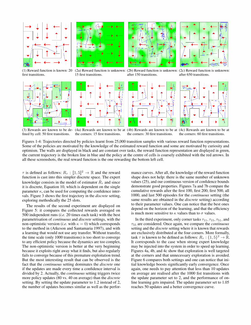
(1) Reward function is known: 20first transitions.
(2a) Reward function is unknown:15 first transitions.
(2b) Reward function is unknown:after 150 transitions.
(2c) Reward function is unknown:after 650 transitions.
(3) Rewards are known to be de-fined by cell: 50 first transitions.
(4a) Rewards are known to be atthe corners: 15 first transitions.
(4b) Rewards are known to be atthe corners: 30 first transitions.
(4c) Rewards are known to be atthe corners: 60 first transitions.
Figures 1-4: Trajectories directed by policies learnt from 25,000 transition samples with various reward function representations.Some of the policies are motivated by the knowledge of the estimated reward function and some are motivated by curiosity andoptimism. The walls are displayed in black and are constant over tasks, the reward function representation are displayed in green,the current trajectory is the broken line in blue and the policy at the centre of cells is coarsely exhibited with the red arrows. Inall these screenshots, the real reward function is the one rewarding the bottom left cell.
⌧ is defined as follows: R⌧
: J1, 5K2 ! R and the rewardfunction is cast into this simpler discrete space. The expertknowledge consists in the model of estimator ˆ
R
⌧
and sinceit is discrete, Equation 10, which is dependent on the singleparameter , can be used for computing the confidence inter-vals. Figure 3 shows the first trajectory in the discrete setting,exploring methodically the 25 slots.
The results of the second experiment are displayed onFigure 5: it compares the collected rewards averaged on500 independent runs (i.e. 20 times each task) with the bestparametrisation of continuous and discrete settings, with thenon-optimistic version (i.e. with = 0) which correspondsto the method in (Atkeson and Santamaria 1997), and witha learning that would not use any transfer. Without transfer,the time scale (only 1000 transitions) is too short to convergeto any efficient policy because the dynamics are too complex.The non-optimistic version is better at the very beginningbecause it exploits right away what it finds, but also regularlyfails to converge because of this premature exploitation trend.But the most interesting result that can be observed is thefact that the continuous setting dominates the discrete oneif the updates are made every time a confidence interval isdivided by 2. Actually, the continuous setting triggers twicemore policy updates (80 vs. 40 on average) than the discrete
setting. By setting the update parameter to 1.2 instead of 2,the number of updates becomes similar as well as the perfor-
mance curves. After all, the knowledge of the reward functionshape does not help: there is the same number of unknownvalues (25), and our continuous version of confidence boundsdemonstrate good properties. Figures 7a and 7b compare thecumulative rewards after the first 100, first 200, first 500, all1000, and last 500 episodes for the continuous setting (thesame results are obtained in the discrete setting) accordingto their parameter values. One can notice that the best onesdepend on the horizon of the learning, and that the efficiencyis much more sensitive to values than to � values.
In the third experiment, only corner tasks ⌧11, ⌧15, ⌧51, and⌧55 are considered. Once again, we compare the continuous
setting and the discrete setting where it is known that rewardsare exclusively distributed at the four corners. More formally,task ⌧ is known to be defined as follows: R
⌧
: {1, 5}2 ! R.It corresponds to the case when strong expert knowledgemay be injected into the system in order to speed up learning.Figures 4a, 4b, and 4c show that exploration is well targetedat the corners and that unnecessary exploration is avoided.Figure 6 compares both settings and one can notice that ini-tial knowledge boosts significantly early convergence. Onceagain, one needs to pay attention that less than 10 updateson average are realised after the 1000 fist transitions withthe update parameter set to 2, and the performance of on-line learning gets impaired. The update parameter set to 1.05reaches 50 updates and a better convergence curve.
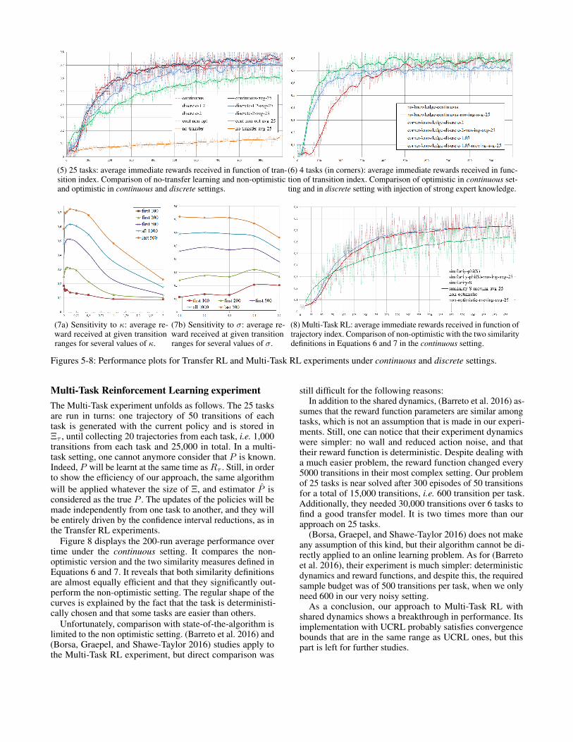
(5) 25 tasks: average immediate rewards received in function of tran-sition index. Comparison of no-transfer learning and non-optimisticand optimistic in continuous and discrete settings.
(6) 4 tasks (in corners): average immediate rewards received in func-tion of transition index. Comparison of optimistic in continuous set-ting and in discrete setting with injection of strong expert knowledge.
(7a) Sensitivity to : average re-ward received at given transitionranges for several values of .
(7b) Sensitivity to �: average re-ward received at given transitionranges for several values of �.
(8) Multi-Task RL: average immediate rewards received in function oftrajectory index. Comparison of non-optimistic with the two similaritydefinitions in Equations 6 and 7 in the continuous setting.
Figures 5-8: Performance plots for Transfer RL and Multi-Task RL experiments under continuous and discrete settings.
Multi-Task Reinforcement Learning experimentThe Multi-Task experiment unfolds as follows. The 25 tasksare run in turns: one trajectory of 50 transitions of eachtask is generated with the current policy and is stored in⌅
⌧
, until collecting 20 trajectories from each task, i.e. 1,000transitions from each task and 25,000 in total. In a multi-task setting, one cannot anymore consider that P is known.Indeed, P will be learnt at the same time as R
⌧
. Still, in orderto show the efficiency of our approach, the same algorithmwill be applied whatever the size of ⌅, and estimator ˆ
P isconsidered as the true P . The updates of the policies will bemade independently from one task to another, and they willbe entirely driven by the confidence interval reductions, as inthe Transfer RL experiments.
Figure 8 displays the 200-run average performance overtime under the continuous setting. It compares the non-optimistic version and the two similarity measures defined inEquations 6 and 7. It reveals that both similarity definitionsare almost equally efficient and that they significantly out-perform the non-optimistic setting. The regular shape of thecurves is explained by the fact that the task is deterministi-cally chosen and that some tasks are easier than others.
Unfortunately, comparison with state-of-the-algorithm islimited to the non optimistic setting. (Barreto et al. 2016) and(Borsa, Graepel, and Shawe-Taylor 2016) studies apply tothe Multi-Task RL experiment, but direct comparison was
still difficult for the following reasons:In addition to the shared dynamics, (Barreto et al. 2016) as-
sumes that the reward function parameters are similar amongtasks, which is not an assumption that is made in our experi-ments. Still, one can notice that their experiment dynamicswere simpler: no wall and reduced action noise, and thattheir reward function is deterministic. Despite dealing witha much easier problem, the reward function changed every5000 transitions in their most complex setting. Our problemof 25 tasks is near solved after 300 episodes of 50 transitionsfor a total of 15,000 transitions, i.e. 600 transition per task.Additionally, they needed 30,000 transitions over 6 tasks tofind a good transfer model. It is two times more than ourapproach on 25 tasks.
(Borsa, Graepel, and Shawe-Taylor 2016) does not makeany assumption of this kind, but their algorithm cannot be di-rectly applied to an online learning problem. As for (Barretoet al. 2016), their experiment is much simpler: deterministicdynamics and reward functions, and despite this, the requiredsample budget was of 500 transitions per task, when we onlyneed 600 in our very noisy setting.
As a conclusion, our approach to Multi-Task RL withshared dynamics shows a breakthrough in performance. Itsimplementation with UCRL probably satisfies convergencebounds that are in the same range as UCRL ones, but thispart is left for further studies.
ReferencesAntos, A.; Szepesvári, C.; and Munos, R. 2007. Value-iterationbased fitted policy iteration: learning with a single trajectory.In Proceedings of the 1st IEEE International Symposium on Ap-
proximate Dynamic Programming and Reinforcement Learning
(ADPRL), 330–337. IEEE.Atkeson, C. G., and Santamaria, J. C. 1997. A comparison ofdirect and model-based reinforcement learning. In Proceedings
of the 14th International Conference on Robotics and Automa-
tion, 3557–3564. IEEE Press.Auer, P., and Ortner, R. 2007. Logarithmic online regret boundsfor undiscounted reinforcement learning. In Proceedings of the
21st Annual Conference on Neural Information Processing Sys-
tems (NIPS), volume 19, 49.Barreto, A.; Munos, R.; Schaul, T.; and Silver, D. 2016. Suc-cessor features for transfer in reinforcement learning. arXiv
preprint arXiv:1606.05312.Borsa, D.; Graepel, T.; and Shawe-Taylor, J. 2016. Learn-ing shared representations in multi-task reinforcement learning.arXiv preprint arXiv:1603.02041.Brafman, R. I., and Tennenholtz, M. 2002. R-max: a gen-eral polynomial time algorithm for near-optimal reinforcementlearning. Journal of Machine Learning Research 3(Oct):213–231.Chandramohan, S.; Geist, M.; and Pietquin, O. 2010. Optimiz-ing spoken dialogue management with fitted value iteration. InProceedings of the 10th Annual Conference of the International
Speech Communication Association (Interspeech), 86–89.Ernst, D.; Geurts, P.; and Wehenkel, L. 2005. Tree-based batchmode reinforcement learning. Journal of Machine Learning
Research 503–556.Genevay, A., and Laroche, R. 2016. Transfer learning foruser adaptation in spoken dialogue systems. In Proceedings of
the 15th International Conference on Autonomous Agents and
Multi-Agent Systems (AAMAS). International Foundation forAutonomous Agents and Multiagent Systems.Holm, S. 1979. A simple sequentially rejective multiple testprocedure. Scandinavian journal of statistics 65–70.Houthooft, R.; Chen, X.; Duan, Y.; Schulman, J.; De Turck, F.;and Abbeel, P. 2016. Curiosity-driven exploration in deepreinforcement learning via bayesian neural networks. arXiv
preprint arXiv:1605.09674.Kearns, M., and Singh, S. 2002. Near-optimal reinforcementlearning in polynomial time. Machine Learning 49(2-3):209–232.Lakshmanan, K.; Ortner, R.; and Ryabko, D. 2015. Improvedregret bounds for undiscounted continuous reinforcement learn-ing. In Proceedings of The 32nd International Conference on
Machine Learning (ICML), volume 37, 524–532.Laroche, R.; Putois, G.; Bretier, P.; and Bouchon-Meunier, B.2009. Hybridisation of expertise and reinforcement learning indialogue systems. In Proceedings of the 9th Annual Conference
of the International Speech Communication Association (Inter-
speech), 2479–2482.Lazaric, A. 2012. Transfer in reinforcement learning: a frame-work and a survey. In Reinforcement Learning. Springer. 143–173.
Lemon, O., and Pietquin, O. 2012. Data-Driven Methods for
Adaptive Spoken Dialogue Systems: Computational Learning
for Conversational Interfaces . Springer.Lopes, M.; Lang, T.; Toussaint, M.; and Oudeyer, P.-Y. 2012.Exploration in model-based reinforcement learning by empiri-cally estimating learning progress. In Proceedings of the 26th
Annual Conference on Neural Information Processing Systems
(NIPS), 206–214.Mnih, V.; Kavukcuoglu, K.; Silver, D.; Graves, A.; Antonoglou,I.; Wierstra, D.; and Riedmiller, M. 2013. Playing atari withdeep reinforcement learning. arXiv preprint arXiv:1312.5602.Mnih, V.; Kavukcuoglu, K.; Silver, D.; Rusu, A. A.; Veness, J.;Bellemare, M. G.; Graves, A.; Riedmiller, M.; Fidjeland, A. K.;Ostrovski, G.; et al. 2015. Human-level control through deepreinforcement learning. Nature 518(7540):529–533.Moore, A. W., and Atkeson, C. G. 1993. Prioritized sweeping:Reinforcement learning with less data and less time. Machine
Learning 13(1):103–130.Ng, A., and Russell, S. 2000. Algorithms for inverse reinforce-ment learning. In in Proceedings of the 17th International Con-
ference on Machine Learning (ICML), 663–670. Morgan Kauf-mann.Ortner, R., and Ryabko, D. 2012. Online regret bounds forundiscounted continuous reinforcement learning. In Proceed-
ings of the 26th Annual Conference on Neural Information Pro-
cessing Systems (NIPS), 1763–1771.Osband, I.; Roy, B. V.; and Wen, Z. 2016. Generalization andexploration via randomized value functions. In Proceedings of
the 33rd International Conference on Machine Learning, ICML
2016, 2377–2386.Romoff, J.; Bengio, E.; and Pineau, J. 2016. Deep conditionalmulti-task learning in atari.Scheffe, H. 1999. The analysis of variance, volume 72. JohnWiley & Sons.Silver, D.; Huang, A.; Maddison, C. J.; Guez, A.; Sifre, L.;van den Driessche, G.; Schrittwieser, J.; Antonoglou, I.; Pan-neershelvam, V.; Lanctot, M.; et al. 2016. Mastering thegame of go with deep neural networks and tree search. Nature
529(7587):484–489.Sutton, R. S., and Barto, A. G. 1998. Reinforcement Learning:
An Introduction (Adaptive Computation and Machine Learn-
ing). The MIT Press.Szepesvári, C. 2010. Algorithms for reinforcement learning.Synthesis lectures on artificial intelligence and machine learn-
ing 4(1):1–103.Taylor, M. E., and Stone, P. 2009. Transfer learning for re-inforcement learning domains: A survey. Journal of Machine
Learning Research 10:1633–1685.Taylor, M. E.; Stone, P.; and Liu, Y. 2007. Transfer learning viainter-task mappings for temporal difference learning. Journal
of Machine Learning Research 8(Sep):2125–2167.Tesauro, G. 1995. Td-gammon: A self-teaching backgammonprogram. In Applications of Neural Networks. Springer. 267–285.Tikhonov, A. N. 1963. Regularization of incorrectly posedproblems. Soviet Mathematics Doklady.