Eemeli Saari

TREND ANALYSIS IN AI RESEARCHOVER TIME USING NLP TECHNIQUES

Signal ProcessingBachelor of Science Thesis

June 2019

i

ABSTRACT

Eemeli Saari: Trend Analysis in AI Research over time Using NLP TechniquesBachelor of Science ThesisTampere UniversityDegree Programme in Computing and Electrical Engineering, BScJune 2019

The dramatic rise in the number of publications in machine learning related studies poses achallenge for companies and new researchers when they want to focus their resources effectively.This thesis aims to provide an automatic pipeline to extract the most relevant trends in the machinelearning field. I applied unsupervised topic modeling methods to discover research trends from fullNIPS conference papers from 1987 to 2018. By comparing the Latent Dirichlet Allocation (LDA)topic model with a model utilizing semantic word vectors (sHDP), it was shown that the LDAperformed better in both quality and coherence. Using the LDA, 50 topics were extracted andinterpreted to match the key concepts in the conference publications. The results revealed threedistinct eras in the NIPS history as well as the steady shift away from the neural informationprocessing roots towards deep learning.

Keywords: natural language processing, NLP, topic modeling, word embedding, trend analysis,scientometric study

The originality of this thesis has been checked using the Turnitin OriginalityCheck service.

ii

PREFACE

This thesis was written as a part of Bachelor of Science program in the spring 2019. Selectingthis subject for my work from a variety of other interesting subjects was due to my pre-existinginterest towards Natural Language Processing. First and foremost, I would like to thank my in-structor Nataliya Strokina for all the support and advice throughout the spring as well as AssistantProfessor Okko Räsänen for his helpful comments and interest towards the work. I also would liketo thank my other half for all the patience along the way.

Tampere, 5th June 2019

Eemeli Saari

iii

CONTENTS

List of Figures . . . . . . . . . . . . . . . . . . . . . . . . . . . . . . . . . . . . . . . . . . . iv

List of Tables . . . . . . . . . . . . . . . . . . . . . . . . . . . . . . . . . . . . . . . . . . . . v

List of Symbols and Abbreviations . . . . . . . . . . . . . . . . . . . . . . . . . . . . . . . . vi

1 Introduction . . . . . . . . . . . . . . . . . . . . . . . . . . . . . . . . . . . . . . . . . . . 1

2 Prior Related Work . . . . . . . . . . . . . . . . . . . . . . . . . . . . . . . . . . . . . . 22.1 Topic Modeling . . . . . . . . . . . . . . . . . . . . . . . . . . . . . . . . . . . . . . 22.2 Word Embedding . . . . . . . . . . . . . . . . . . . . . . . . . . . . . . . . . . . . . 32.3 Topic Modeling over time . . . . . . . . . . . . . . . . . . . . . . . . . . . . . . . . 4

3 Methods . . . . . . . . . . . . . . . . . . . . . . . . . . . . . . . . . . . . . . . . . . . . . 53.1 Topic modeling methods . . . . . . . . . . . . . . . . . . . . . . . . . . . . . . . . . 5

3.1.1 Latent Dirichlet Allocation . . . . . . . . . . . . . . . . . . . . . . . . . . . 53.1.2 Spherical Hierarchical Dirichlet Processes . . . . . . . . . . . . . . . . . . . 6

3.2 Word Representation . . . . . . . . . . . . . . . . . . . . . . . . . . . . . . . . . . . 73.3 Over time . . . . . . . . . . . . . . . . . . . . . . . . . . . . . . . . . . . . . . . . . 8

4 Trend Analysis . . . . . . . . . . . . . . . . . . . . . . . . . . . . . . . . . . . . . . . . . 104.1 Data . . . . . . . . . . . . . . . . . . . . . . . . . . . . . . . . . . . . . . . . . . . . 104.2 Word Embedding . . . . . . . . . . . . . . . . . . . . . . . . . . . . . . . . . . . . . 114.3 Model . . . . . . . . . . . . . . . . . . . . . . . . . . . . . . . . . . . . . . . . . . . 114.4 Results and Analysis . . . . . . . . . . . . . . . . . . . . . . . . . . . . . . . . . . . 11

4.4.1 Discovering Topics . . . . . . . . . . . . . . . . . . . . . . . . . . . . . . . . 124.4.2 Topic Distribution over time . . . . . . . . . . . . . . . . . . . . . . . . . . 12

5 Conclusion . . . . . . . . . . . . . . . . . . . . . . . . . . . . . . . . . . . . . . . . . . . 18

References . . . . . . . . . . . . . . . . . . . . . . . . . . . . . . . . . . . . . . . . . . . . . . 19

Appendix A Appendix . . . . . . . . . . . . . . . . . . . . . . . . . . . . . . . . . . . . . . 22

iv

LIST OF FIGURES

3.1 Graphical representation of LDA model. The box M represents documents and Nthe choice of topic and word within the document. . . . . . . . . . . . . . . . . . . 6

3.2 Simplified graphical representation of sHDP model [24]. The model assumes Mdocuments in the corpus with N words and countably infinite topics represented by(µk, κk). . . . . . . . . . . . . . . . . . . . . . . . . . . . . . . . . . . . . . . . . . . 7

3.3 Continuous Bag-of-word model. . . . . . . . . . . . . . . . . . . . . . . . . . . . . . 7

4.1 Number of documents and average token count from NIPS between 1987 and 2018processed dataset. . . . . . . . . . . . . . . . . . . . . . . . . . . . . . . . . . . . . 10

4.2 Topic distributions for NIPS 1987-2018 corpora. Each color represents one year’sportion of overall topic distribution. . . . . . . . . . . . . . . . . . . . . . . . . . . 12

4.3 Yearly topic distributions for LDA model. Topics are shown in ascending order fromthe first (bottom) to the last (top). . . . . . . . . . . . . . . . . . . . . . . . . . . . 14

4.4 Top 25 rising labeled topics from NIPS 1987-2018. . . . . . . . . . . . . . . . . . . 154.5 Bottom 25 falling labeled topics from NIPS 1987-2018. . . . . . . . . . . . . . . . . 164.6 Yearly topic distributions and similarities between years. Green marks the era of

neuroscience, red marks the algorithmic era, and cyan represents the deep learningera. . . . . . . . . . . . . . . . . . . . . . . . . . . . . . . . . . . . . . . . . . . . . . 17

A.1 Yearly topic distributions for sHDP model. Topics are shown in ascending orderfrom the first (bottom) to the last (top). . . . . . . . . . . . . . . . . . . . . . . . . 22

v

LIST OF TABLES

4.1 Average topic coherence for LDA and sHDP with different hyperparameters. . . . . 114.2 Top 10 words and interpreted topics in alphabetical order. . . . . . . . . . . . . . . 13

A.1 Top 10 words for sHDP(α = 0.1, γ = 1.5) topics. . . . . . . . . . . . . . . . . . . . 23

vi

LIST OF SYMBOLS AND ABBREVIATIONS

BERT Bidirectional Encoder Represen-tations fromTransformers

BRNN Bidirectional Recurrent Neural Network

CBOW Continuous Bag-of-word

GAN Generative Adversial NetworkGPU Graphical Processing Unit

HDP Hierarchical Dirichlet Processes

JSD Jensen-Shannon Divergence

KLD Kullback-Leibler Divergence

LDA Latent Dirichlet AllocationLSA Latent Semantic AnalysisLSTM Long Short-Term Memory

MAP Maximum A Posterior

nHDP nested Hierarchical Dirichlet ProcessesNIPS Neural Information Processing SystemsNLP Natural Language ProcessingNNLM Neural Net Language Model

PDF Portable Document FormatPMI Pointwise Mutual Information

RNN Recurrent Neural Network

SGNS Skip-Gram Negative SamplingsHDP spherical Hierarchical Dirichlet ProcessesSVD Singular Value DecompositionSVM Support-Vector Machine

θ Topic distribution

vii

vMF von Mises-Fisher

ψ Word distribution

1

1 INTRODUCTION

Available information in the world has grown exponentially since the introduction of the worldwide web [1]. This phenomena is seen in different research domains as an increase in the numberof publications yearly and as an acceleration in the development of research in general. In the fieldof machine learning and artificial intelligence particularly, the acceleration has made the overallimage of the current trends fuzzy. This has lead to a problem for new researchers and companieswhen they want to invest their time and resources efficiently.

The Natural Language Processing (NLP) offers a set of tools capable of deriving knowledgefrom large collections of text data. Topic modeling [2] is one area of interest in the NLP researchwhich focuses on the automatic discovery of hidden structures in texts. The method attempts todescribe a collection of text documents as a collection of word topics using statistical methodology.Topic models have been applied to various tasks such as detecting suspicious e-mails [3], Twittercontent classification [4], and clustering scientific papers [5]. Though powerful in many tasks, thestatistical approach of topic models is often limited to semantic structures found in the naturallanguage. To represent these structures efficiently a number of word embedding methods havebeen introduced [6][7][8][9]. These methods leverage the learned semantic structures from the datato various tasks such as machine translation [10] and sentiment analysis [11]. Topic modeling hasalso seen improvements when combined with word vector representations [12].

The main purpose of this thesis is to provide a pipeline for automatic topic discovery andanalysis using the state-of-the-art tools. In this work I aim to apply the pipeline for unsupervisedscientometric study to detect trends in machine learning over the years. Using the knowledge minedin this way I will hope to discover some of the latent paths and directions in the field. Unlike mostresearch that involves scientific paper abstracts, I will use full publications as data. Secondary aimfor this study is to detect and compare the impacts of combining word representations with topicmodeling.

Chapter 2. introduces the related works on different topic, word representations models andcombinatory models, as well as topic modeling over time. Chapter 3. presents the proposed pipelineand the used methods in detail. Chapter 4. introduces the data and the results for the conductedtrend analysis study, and final Chapter 5. presents the results and future improvements.

2

2 PRIOR RELATED WORK

Most of the modern approaches in NLP are based on the distributional hypothesis [13] thatwords occurring in the same context tend to have similar meanings. This hypothesis lays the foun-dation for machine learning and pattern recognition in the computational linguistics and naturallanguage processing.

2.1 Topic Modeling

Latent Dirichlet Allocation (LDA) [14] is the most commonly used topic modeling method thataims to find a set of latent topics from a given corpora. The objective of the LDA is to representeach document in the corpora as a probability distribution over topics. Each topic distribution iscomposed of probability distribution over all words in the vocabulary. From these distributionsone can observe high probability words and derive understanding of each document content. Thealgorithm of the LDA model is generative and can be trained in batches with large datasets. Thisenables the model to generalize to the previously unseen documents. However, the task to infer theword and topic probabilities while iterating is intractable, as there exists multiple random variables.As the answer, the authors of LDA applied the Variational inference [15]. Other methods suchas Gibbs sampling [16] are also widely used. LDA can be described as a general statistic modelmeaning that it can be applied to various fields with differing data other than text [17]. LDAis based on the probabilistic Latent Semantic Analytics (pLSA) [18] and has been described asMaximum A Posterior (MAP) estimation for the LDA model [19].

Capturing informative high level topics from text data is not limited to the LDA model. Sincethe process of using LDA often defaults to model selection and hyperparameter optimization,some nonparametric alternative elaborations have been proposed. One of these methods is HDP(Hierarchical Dirichlet Processes) [20] that uses Bayesian Dirichlet process [21] to extend the LDAin topic modeling tasks. The performance of the HDP model matched the best performance ofthe LDA without any model selection required. More recent elaboration nHDP [22] attempts toanswer the inference scalability problem of topic models for very large datasets. This methodcomposes the text efficiently as topic hierarchies, resulting in a tree-structure representation. Thenonparametric nature of HDP models is advantageous in various autonomous tasks where the priorknowledge of the data can be unknown or when the resources limit the model selection.

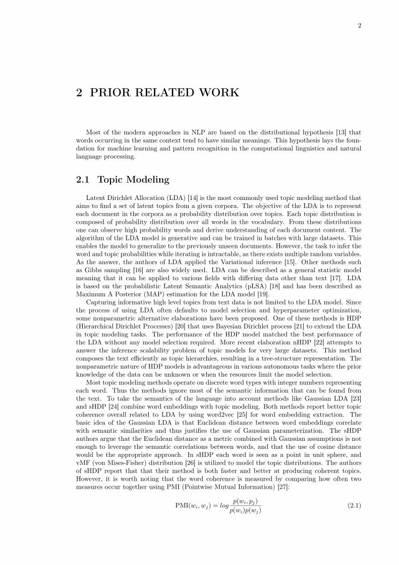
Most topic modeling methods operate on discrete word types with integer numbers representingeach word. Thus the methods ignore most of the semantic information that can be found fromthe text. To take the semantics of the language into account methods like Gaussian LDA [23]and sHDP [24] combine word embeddings with topic modeling. Both methods report better topiccoherence overall related to LDA by using word2vec [25] for word embedding extraction. Thebasic idea of the Gaussian LDA is that Euclidean distance between word embeddings correlatewith semantic similarities and thus justifies the use of Gaussian parameterization. The sHDPauthors argue that the Euclidean distance as a metric combined with Gaussian assumptions is notenough to leverage the semantic correlations between words, and that the use of cosine distancewould be the appropriate approach. In sHDP each word is seen as a point in unit sphere, andvMF (von Mises-Fisher) distribution [26] is utilized to model the topic distributions. The authorsof sHDP report that that their method is both faster and better at producing coherent topics.However, it is worth noting that the word coherence is measured by comparing how often twomeasures occur together using PMI (Pointwise Mutual Information) [27]:

PMI(wi, wj) = logp(wi, pj)

p(wi)p(wj)(2.1)

3

It has been shown that the PMI correlates well with the human judgement on topic quality [28]providing a good basis for model selection. Although widely used, it should be noted that humanevaluation is always needed to determine the quality of the topics.

2.2 Word Embedding

The ability to represent words and capture meaningful syntactic and semantic information oflanguage [29] has made pre-trained word vectors a key component in modern NLP. A number ofmethods have been used in the past to learn word embeddings from simple N-Gram models [30] tostatistical count base Latent Semantic Analysis (LSA) [31]. Modern methods utilize both shallow[25] and deep [8][9] neural networks to train the embeddings from large collections of data. Themain idea of these models is to leverage learned semantic feature vectors to downstream tasks suchas question answering and document classification.

Predictive learning algorithms that represent words as continuous vectors have been shown tooutperform some of the traditional count-based methods [32]. The main advantage comes fromthe ability of the embeddings to represent meaningful semantic relationships in encoded vectorspace. In this space analogy such as "Helsinki is to Stockholm as Finland is to Sweden" should beencoded in the equation

Helsinki− Stockholm = Finland− Sweden

Vector space also enables the query for similarity estimates. For example Euclidean distance is ametric which is shown to correlate semantic similiarities between two word embeddings. Word2vecauthors also used cosine similarity to find nearest neighbors in the word vector space.

Skip-Gram model and Continuous Bag-of-Words (CBOW) model provided in Google’s word2vecare commonly used methods for learning word embeddings. Both models use an architecture similarto the feedforward Neural Net Language Model (NNLM) [33]. The feedforward NNLM architectureconsists of input, projection, hidden and softmax output layer. Skip-Gram model and CBOWmodel remove the non-linear hidden layer from NNLM and share the projection layer with all ofthe words, meaning that the word vectors are averaged. The principle for word2vector modelsis to stream the data window around a pivot word. In this way the model learns which wordsappear in similar context, unlike the NNLM which learns what words predict the pivot word. TheSkip-Gram model and CBOW model differ in the learning objective. Skip-Gram model, in short,attempts to predict the surrounding context words around target word, whereas CBOW modelpredicts the target word based on the surrounding context. Word2vec models can also replace thesoftmax layer with efficient negative sampling layer to speed up the learning process.

The word2vec models have had multiple variations over the years. The most notable and widelyused one is the Standford’s GloVe [7] model that takes advantage of the global count-based statisticsfrom the target corpora. This count-based method utilizes the global matrix factorization that hasroots all the way back to the LSA [31]. LSA decomposes large matrices to capture statisticalinformation from the corpora using SVD (Singular Value Decomposition) [34]. GloVe utilizes asimiliar approach to LSA by composing co-occurrence matrices in both the local window and theglobal context. These co-occurrence matrices are used to form a set of probabilities for a wordto appear in a given context. Then the model is trained to optimize the log mean squared errorbetween the predicted probabilities and the observed probabilities. Interestingly the GloVe modelis very similar to the word2vec skip-gram model that implicitly decomposes co-occurance matrixwhen streaming over windows of words [35].

The current state-of-the-art method for word embedding models is Bidirectional Encoder Rep-resentations from Transformers (Bert) [9] that uses a powerful Transformer architecture [36] toembed both sentences and words from corpora. BERT attempts to directly solve a polysemousword problem that a word such as ”apple” may have meanings depending on whether it appears inthe context of information technology or in agriculture. Models like ELMo [8] solve this problemby training the Bidirectional Recurrent Neural Network (BRNN) [37] with LSTM layers [38] topredict target word based on both previous and future context. BERT utilizes the cloze procedure[39] during the training where words from sentences are masked at random. This forces the modelto consider the entire context simultaneously, which the authors report as one of the main factorsfor the outperformance of the model in various benchmark tests. BERT was designed to be usedas a pre-trained base for domain specific transfer learning tasks, for example, data mining for

4

biomedical texts [40].

2.3 Topic Modeling over time

Topic models are used to capture the low-dimensional statistical information about the structureof the data and thus not explicitly model the temporal relationships between topics. This causesthe standard topic models such as LDA to suffer in terms of topic quality with datasets thatusually have been collected over time. For example, in the case of Wikipedia, corpora the datamight contain edits over a vastly different timescales and even outdated language and knowledge.Itis desirable to detect these types of data features for many high-end tasks such as trend analysiswhere evolution of topics over time offers valuable information. Standard LDA needs to be extendedto fully capture the topic evolution over time.

The time dimension can be taken into account for topic models in two modeling frameworks.The joint framework integrates the time domain directly into the process of topic modeling. Oneof the methods utilizing this is Topics over time [41] where time is taken into account by applyingcontinuous distribution over timestamps. Topic over time model can thus capture the locality ofgiven topics in time. Discretization of time is used in dynamic topic model [42] where one appliesthe Markov assumption that the state of topics changes in time. Non-joint approach is usuallymore flexible since it does not require radical adjustments to the existing models. The process ofnon-joint topic modeling is usually done using post hoc analysis. The process consists of fittingthe topic model with time-unaware data and then aggregating the results for each time period[16]. This process relies on the assumption that the topics are static and the assumption does notdistinguish whether the meaning or occurrence of the topic has changed.

Topic models applied to timeseries data have offered valuable information in various differentdomains. One of these domains has been scientometrics where mostly quantitative methods havebeen applied to study the citations as graph, and to conclude the importance of the given paperor article. This, however does not take into account the difference between research domains, andthus topic models have been applied to study these properties with more detail. For example thehistory of ideas [43] has been studied in conference publications where the the authors were able todetect rise and fall of topics over time. One of the key outcomes from this study was the observationthat different conferences were converging over time to cover the same topics. Trends have alsobeen studied in different research domains. Also one study focusing on the trends in transportationresearch journals found similarities between different journals and was able to cluster journals usingtopic modelling over time [44].

5

3 METHODS

This chapter explains the methods used in the trend analysis pipeline. The sections are dividedinto three subsections that are applied to the preprocessed data: Building the word representationvectors, topic modeling and interpreting the topics over time. All the steps in the pipeline aretreated as scikit-learn API [45] transformers. In this way the pipeline can be built with differentsteps providing a robust system. Preprocessing steps are described in detail in Chapter 4.

3.1 Topic modeling methods

3.1.1 Latent Dirichlet Allocation

Latent Dirichlet Allocation (LDA) [14] is a Bayesian probabilistic model of a corpus D. Thebasic idea of the model is that each document d in corpus is a mixture over latent topics z, andeach topic is characterized by a distribution over words wn in the vocabulary V . LDA assumesthe following generative process for each d ∈ D

1. Choose the length of documents N ∼ Poisson(ξ).

2. Choose the topic proportion θ ∼ Dir(α)

3. For each word wn ∈ N :

(a) Choose a topic zn ∼Multinomial(θ)

(b) Choose a word wn from P (wn|zd, β), a multinomial probability conditioned on the topiczn.

Here the notation Dir is the Dirichlet distribution function and Multinomial is the Multinomialdistribution function. The parameter α marks the topic Dirichlet prior and β marks the wordDirichlet prior. Several simplification assumptions are made for the basic LDA model. The param-eter N drawn from the Poisson assumption is not needed and the N is thus often marked as thelength of the document. Dimensionality k of the Dirichlet distribution that determines the topic zdimension is assumed to be known and fixed. Since the model also uses a finite vocabulary V , theword probabilities are parameterized by a k × V matrix β. Using the matrix notation probabilityof the ith word in a given document is described as

P (wi) =

k∑j=1

P (wi|zi = j)P (zi = j) (3.1)

where i stands for ith row and j stands for jth column of matrix β. The task of the model is thento obtain an estimate for β that gives high probability to the words that appear in the corpus.The corpus D is analyzed by examining the posterior distribution of β, topic proportion θ and thetopic assignment z in the documents. However, the posteriors cannot be computed directly and istherefore estimated. In the generative model the estimation problem transforms into maximizingthe equation

P (d|α, β) =∫P (θ|α)P (d|β, θ), dθ (3.2)

where β is the hidden parameter to be estimated. The LDA model is shown graphically in Figure3.1.

6

Figure 3.1. Graphical representation of LDA model. The box M represents documents and Nthe choice of topic and word within the document.

The estimation problem in the LDA is an inferential problem over parameter β. This thesisuses the LDA model provided by gensim[46] that utilizes the online implementation of the LDA[47]. In the online version of the LDA, the Variational inference is applied to single documents in astreaming manner. Other proposed inference methods include Gipps sampling and Markov ChainMonte Carlo (MCMC) [16].

3.1.2 Spherical Hierarchical Dirichlet Processes

Spherical Hierarchical Dirichlet Processes (sHDP) [24] is based on the HDP. Instead of the LDA,the sHDP model assumes a non-fixed collection of topics z that are shared across the documents din the corpus C. Using the normalized N dimensional word vector representations the topics arerepresented by topic centers µz ∈N . The model assumes the word vectors as normalized, thus thetopic center µk can be seen as directions on a unit sphere. The model defines the likelihood of thetopic z for word wk

f(wk;µz, κz) = exp(κzµTz wdn)CN (κz) (3.3)

where the von Mises-Fisher (vMF) probability function is used and κz is the concentration of thetopic z. The model captures semantic similarity between topic and words in the log-likelihood ofthe vMF since the µT

z wdn is equal to cosine distance that is used to compare word vectors as well.The factor CN is the normalization constant used in the vMF [48]

CN (κz) :=κN/2−1z

(2π)N/2IN/2−1(κz)(3.4)

sHDP processes the documents in a generative way which is similar to how the LDA process.Topic zdw is selected for the word w of document d from zdw ∼ Multinomial(πd). Using the DirichletProcess to draw πd ∼ DP(α, β) which enables the model to estimate the number of topics from thedata. Differing from LDA, the sHDP draws the parameter β from the stick-breaking distribution[21] β ∼ GEM(γ) where γ is the concentration parameter. Graphical representation for sHDPmodel is shown in Figure 3.2. Inference in the model for latent variables is done using StochasticVariational Mean-field Inference (SVI) [49]. This enables the model to process documents inbatches making it appropriate for large-scale settings. One can observe that the automatic HDP-based approach has some drawbacks. For example, the number of latent variables the model needsto infere is significantly larger compared to LDA.

7

Figure 3.2. Simplified graphical representation of sHDP model [24]. The model assumes Mdocuments in the corpus with N words and countably infinite topics represented by (µk, κk).

3.2 Word Representation

The first step of the pipeline is to compute the word representations for the vocabulary of wordsV . This can be done as a separate step by training with larger dataset or by training sequentiallyas part of the pipeline. Continuous Bag-of-word model [25] is selected for the single purpose ofproviding the word vectors as features for the topic modeling method.

The training objective for the CBOW model is to predict target word wt given a set of contextwords {wt−n, wt−n−1, ..., wt+n−1, wt+n} where the n is the window size. The model consists of theinput, projection, hidden and output layers. Fixed vocabulary size V and hidden layer size of Nis assumed. Figure 3.3 illustrates the architecture of the CBOW model.

Figure 3.3. Continuous Bag-of-word model.

The input words are represented as one-hot encoded V size vectors {x1, x2, ...xC} where C isthe number of words in the context. For the given context word wk ∈ V , the one-hot encoded

8

vector’s unit will have one out of V units 1 and 0 otherwise. The weights between the input layerand the output layer are represented by V × N matrix W . This matrix contains N dimensionalvector representations vw of the associated word of the input layer on each row. The projectionlayer takes the input vectors of the input context and averages them. Computing the hidden layeroutput is thus

h =1

CWT (x1 + x2 + ...+ xC) (3.5)

which essentially copies the kth row for each input vector word from the matrix W and thereforethe equation is reduced to

h =1

C(vw1 + vw2 + ...+ vwC

) (3.6)

The weights of hidden layer to the output layer is represented as N × V matrix W ′. With theweights W ′ the score uj is computed for each word in the vocabulary V with

uj = v′wj

Th (3.7)

where the v′wjis the jth column of the weight matrix W ′. Then softmax is applied to obtain the

posterior distribution of words for all the input vector words wj from formula

P (wj |wI) =exp(v′wj

T v′wI)∑V

j′=1 exp(v′w′j

T v′wI)

(3.8)

which is the training objective for the model to maximize. This process is represented with givenloss function for the output layer yj

E = −logP (wO|wI,1, ..., wI,C) (3.9)

where the wO is the actual observed word and yj is the output layer. This is computed withformula

E = −v′wO· h+ log

V∑j′=1

exp(v′wj

T · h) (3.10)

In the training process both weights W and W ′ are updated [50]. The training becomes compu-tationally more efficient, if for example, hierarchical softmax or the negative sampling are appliedinstead of the standard softmax function.

A common way to process the word vectors for other tasks is to normalize them. For this acommonly used Euclidean norm l2 is used which is defined for word vector x of size N as [51]

|x| =

√ N∑k=1

|xk|2 (3.11)

3.3 Over time

The topic distributions are measured over time in a post hoc way. Models are trained withoutthe time dimension and topics are computed for each document independently. Similar approachto [44] is taken by grouping the documents by year and averaging the distributions over year. Fora topic distribution θtk, at timestep t and topic k is defined as

θtk =

∑Nd=1 θdkΠ(td = t)∑Nd=1 Π(td = t)

(3.12)

where Π(e) = 1 if e is true and 0 otherwise. The topic distribution θt can be thus seen as asignature for given time t. This information over time is further refined to find rising and fallingtopics with the equation

rk =

∑2002t=1897 θ

tk∑2018

t=2003 θtk

(3.13)

9

where the higher rk value indicates a falling topic. The topic distribution signatures can be usedto find similarities between different years ti and tj . The similarity between two time windowsdti,tj is found using Jensen-Shannon distance [52], namely

dti,tj =√

JSD(θti , θtj ) (3.14)

where JSD is known as Jensen-Shannon divergence which is used to quantify the difference betweentwo distributions θ and θ′

JSD(θti , θtj ) =1

2KLD(θti , θ) +

1

2KLD(θtj , θ) (3.15)

where the θ = 12 (θ+ θ′). The KLD used in the JSD is Kullback-Leibler divergen [53] and is define

as

KLD(θ, θ′) =

K∑k=1

θklogθkθ′k

(3.16)

for any given distribution θ. Using this metric allows different time periods t to be explored byapplying hierarchical clustering similar to [44] where different journals were compared.

10

4 TREND ANALYSIS

4.1 Data

Scientific conferences are often considered to represent the current state-of-the-art in scientificdevelopment. Related studies analysing the trends in the conferences have used information fromabstracts as a proxy to the whole article [43]. This has been justified by the assertion that abstractcontains enough keywords about the document and thus represents the overall research theme well[54]. However, in this thesis I expect some of the latent trends to be missed if only the abstractsare used. For example, the studies and methods cited in the sections covering related works andmethods could contain some valuable information.

Neural Information Processing Systems Conference (NIPS) is a conference for machine learningand computational neuroscience and is held at high prestige amongst researchers. For this thesis,proceeding papers from years 1987 to 2018 were scraped from the website1 using the Beautifulsoup2.PDF documents were then converted to raw text format using pdftotext3, and those documentswhich were corrupted by the conversion process were removed manually. The number of documentscollected was 8233 and the yearly results are shown in Figure 4.1a. A similar observation in thestudy on transportation field [44] can be seen as the number of papers have increased rapidly.

1988

1990

1992

1994

1996

1998

2000

2002

2004

2006

2008

2010

2012

2014

2016

2018

Years

0

250

500

750

1000

Docu

men

ts

(a) Document counts.

1988

1990

1992

1994

1996

1998

2000

2002

2004

2006

2008

2010

2012

2014

2016

2018

Years

0

1000

2000

3000

Token

count

aver

age

(b) Token counts.

Figure 4.1. Number of documents and average token count from NIPS between 1987 and 2018processed dataset.

The preprocessing of the documents was done using a parsing module found in the gensim[46]. The process included parsing tags, punctuations, multiple whitespaces, numeric values aswell as removing the words under three characters long, and the common stopwords. Words thatappeared in less than 20 documents and in more than 75% of the documents overall were alsoremoved. Lastly the parsed documents were split with whitespace into discrete token vectors.With the preprocessed data a dictionary of V = 18513 words was built. I chose to exclude thestemming and lemmatization from the preprocess as they were not used in the other trend analysispapers either [44][54]. The results for average parsed token counts yearly are shown in Figure 4.1b.

1https://papers.nips.cc/2https://www.crummy.com/software/BeautifulSoup/3https://www.xpdfreader.com/

11

4.2 Word Embedding

One aim of this thesis was to investigate the impact of using the word embeddings as partof the topic modeling. The word vector model was trained from scratch with NIPS documentsfrom 1987 to 2018. For this experiment I chose the CBOW model provided in gensim with defaulthyperparameters. Window size was set to 15 with the target embedding vector length 50, andword vectors were normalized using Formula 3.11 according to the original sHDP paper [24].

4.3 Model

First, I experimented with the sHDP4 to see whether or not the promised higher PMI scorewould transfer well into the trend analysis task. Preprocessed token vectors were transformed intoBag-of-Word representations where each token was assigned a integer label, and the number oftoken occurrences from the document were counted. For the sHDP model, counts were replacedwith the words vector representations using the CBOW model. The sHDP was trained with bothdefault hyperparameters and experimented with lower α and γ values. The sHDP implementationwas able to reach a maximum of 60 topics until unstable results occurred.

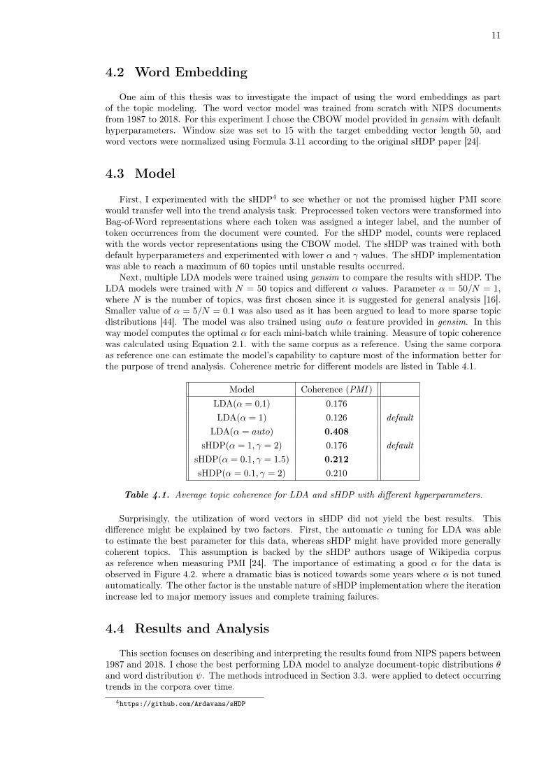
Next, multiple LDA models were trained using gensim to compare the results with sHDP. TheLDA models were trained with N = 50 topics and different α values. Parameter α = 50/N = 1,where N is the number of topics, was first chosen since it is suggested for general analysis [16].Smaller value of α = 5/N = 0.1 was also used as it has been argued to lead to more sparse topicdistributions [44]. The model was also trained using auto α feature provided in gensim. In thisway model computes the optimal α for each mini-batch while training. Measure of topic coherencewas calculated using Equation 2.1. with the same corpus as a reference. Using the same corporaas reference one can estimate the model’s capability to capture most of the information better forthe purpose of trend analysis. Coherence metric for different models are listed in Table 4.1.

Model Coherence (PMI )LDA(α = 0.1) 0.176LDA(α = 1) 0.126 default

LDA(α = auto) 0.408sHDP(α = 1, γ = 2) 0.176 default

sHDP(α = 0.1, γ = 1.5) 0.212sHDP(α = 0.1, γ = 2) 0.210

Table 4.1. Average topic coherence for LDA and sHDP with different hyperparameters.

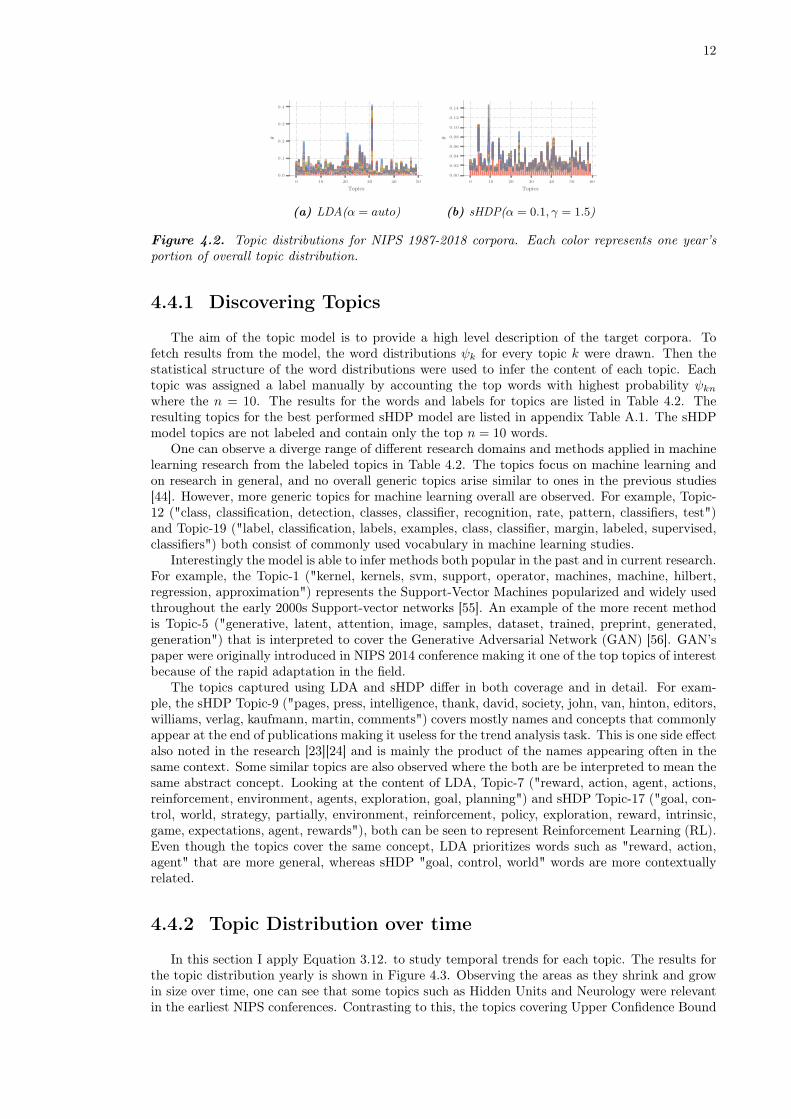
Surprisingly, the utilization of word vectors in sHDP did not yield the best results. Thisdifference might be explained by two factors. First, the automatic α tuning for LDA was ableto estimate the best parameter for this data, whereas sHDP might have provided more generallycoherent topics. This assumption is backed by the sHDP authors usage of Wikipedia corpusas reference when measuring PMI [24]. The importance of estimating a good α for the data isobserved in Figure 4.2. where a dramatic bias is noticed towards some years where α is not tunedautomatically. The other factor is the unstable nature of sHDP implementation where the iterationincrease led to major memory issues and complete training failures.

4.4 Results and Analysis

This section focuses on describing and interpreting the results found from NIPS papers between1987 and 2018. I chose the best performing LDA model to analyze document-topic distributions θand word distribution ψ. The methods introduced in Section 3.3. were applied to detect occurringtrends in the corpora over time.

4https://github.com/Ardavans/sHDP

12

0 10 20 30 40 50

Topics

0.0

0.1

0.2

0.3

0.4

θ

(a) LDA(α = auto)

0 10 20 30 40 50 60

Topics

0.00

0.02

0.04

0.06

0.08

0.10

0.12

0.14

θ

(b) sHDP(α = 0.1, γ = 1.5)

Figure 4.2. Topic distributions for NIPS 1987-2018 corpora. Each color represents one year’sportion of overall topic distribution.

4.4.1 Discovering Topics

The aim of the topic model is to provide a high level description of the target corpora. Tofetch results from the model, the word distributions ψk for every topic k were drawn. Then thestatistical structure of the word distributions were used to infer the content of each topic. Eachtopic was assigned a label manually by accounting the top words with highest probability ψkn

where the n = 10. The results for the words and labels for topics are listed in Table 4.2. Theresulting topics for the best performed sHDP model are listed in appendix Table A.1. The sHDPmodel topics are not labeled and contain only the top n = 10 words.

One can observe a diverge range of different research domains and methods applied in machinelearning research from the labeled topics in Table 4.2. The topics focus on machine learning andon research in general, and no overall generic topics arise similar to ones in the previous studies[44]. However, more generic topics for machine learning overall are observed. For example, Topic-12 ("class, classification, detection, classes, classifier, recognition, rate, pattern, classifiers, test")and Topic-19 ("label, classification, labels, examples, class, classifier, margin, labeled, supervised,classifiers") both consist of commonly used vocabulary in machine learning studies.

Interestingly the model is able to infer methods both popular in the past and in current research.For example, the Topic-1 ("kernel, kernels, svm, support, operator, machines, machine, hilbert,regression, approximation") represents the Support-Vector Machines popularized and widely usedthroughout the early 2000s Support-vector networks [55]. An example of the more recent methodis Topic-5 ("generative, latent, attention, image, samples, dataset, trained, preprint, generated,generation") that is interpreted to cover the Generative Adversarial Network (GAN) [56]. GAN’spaper were originally introduced in NIPS 2014 conference making it one of the top topics of interestbecause of the rapid adaptation in the field.

The topics captured using LDA and sHDP differ in both coverage and in detail. For exam-ple, the sHDP Topic-9 ("pages, press, intelligence, thank, david, society, john, van, hinton, editors,williams, verlag, kaufmann, martin, comments") covers mostly names and concepts that commonlyappear at the end of publications making it useless for the trend analysis task. This is one side effectalso noted in the research [23][24] and is mainly the product of the names appearing often in thesame context. Some similar topics are also observed where the both are be interpreted to mean thesame abstract concept. Looking at the content of LDA, Topic-7 ("reward, action, agent, actions,reinforcement, environment, agents, exploration, goal, planning") and sHDP Topic-17 ("goal, con-trol, world, strategy, partially, environment, reinforcement, policy, exploration, reward, intrinsic,game, expectations, agent, rewards"), both can be seen to represent Reinforcement Learning (RL).Even though the topics cover the same concept, LDA prioritizes words such as "reward, action,agent" that are more general, whereas sHDP "goal, control, world" words are more contextuallyrelated.

4.4.2 Topic Distribution over time

In this section I apply Equation 3.12. to study temporal trends for each topic. The results forthe topic distribution yearly is shown in Figure 4.3. Observing the areas as they shrink and growin size over time, one can see that some topics such as Hidden Units and Neurology were relevantin the earliest NIPS conferences. Contrasting to this, the topics covering Upper Confidence Bound

13

Topic-14 Approximation theorem approximation polynomial properties proof definition continuous property condition positiveTopic-47 Bayesian bayesian prior noise posterior covariance uncertainty likelihood priors variance processesTopic-8 Belief Propagation energy belief inference propagation factor message graphical field map variableTopic-12 Classification class classification detection classes classifier recognition rate pattern classifiers testTopic-36 Clustering clustering cluster clusters means points partition spectral centers partitioning setsTopic-24 Cost Optimization search cost active user query greedy items selection users optimizationTopic-43 Datasets features feature dataset datasets accuracy table test score validation classificationTopic-32 Distance metrics distance metric similarity causal nearest neighbor distances pairwise euclidean neighborsTopic-20 Distributed computing memory distributed communication parallel bit bits code binary precision sizeTopic-34 Domain Adaptation target domain source adaptation domains sources shift targets transfer distributionsTopic-16 Entropy entropy divergence mutual measure ensemble measures log compression distributions maximumTopic-25 Estimations estimation estimator estimate variance estimates estimators rate statistics density estimatingTopic-6 Face Images image images face pixel shape pixels vision matching recognition poseTopic-17 Filters filter filters basis natural coding sparse coefficients ica representation reconstructionTopic-40 Gamification game strategy expert strategies equilibrium experts utility price best playTopic-5 Generative Adversarial Network generative latent attention image samples dataset trained preprint generated generationTopic-27 Grandient optimization gradient optimization convergence stochastic descent convex step rate update iterationTopic-2 Graphs graph graphs edge edges nodes node structure degree connected directedTopic-45 Human/Subjects human subjects decision trial trials subject experiment task cognitive behaviorTopic-49 Image segmentation image segmentation map cvpr vision semantic maps scale proposed detectionTopic-15 Inference inference log variational latent posterior likelihood approximate approximation bound stochasticTopic-19 Labels label classification labels examples class classifier margin labeled supervised classifiersTopic-11 Loss/Predict loss prediction risk regression predictions structured output predict predictor predictedTopic-44 Markov Models sequence states sequences markov transition hidden dynamic series processes lengthTopic-39 Matrix factorization rank matrices low norm entries decomposition column columns factorization spectralTopic-41 Mixture models mixture likelihood distributions density log conditional parameter estimation components mixturesTopic-10 Motion/Video motion video position frame flow tracking direction frames motor trajectoryTopic-31 Hidden Units units output hidden weights unit weight net inputs generalization layerTopic-21 Neurology cells cell activity brain cortex visual spatial cortical connections patternsTopic-35 Neurons/Synapses neurons neuron spike synaptic firing synapses spikes spiking rate ruleTopic-46 Objects object objects visual scene features view categories category recognition representationTopic-33 Optimization optimization solution constraints convex constraint max objective min dual solutionsTopic-23 Principal Component Analysis pca projection component subspace principal components eigenvalues covariance dimensionality vectorsTopic-37 Policy learning policy reinforcement policies mdp decision action states control iteration rewardTopic-28 Recurrent layers layer layers trained architecture output recurrent hidden weights size architecturesTopic-7 Reinforcement learning reward action agent actions reinforcement environment agents exploration goal planningTopic-4 Rules/Knowledge rules rule knowledge program probabilistic representation question language variable reasoningTopic-1 Support-Vector Machine kernel kernels svm support operator machines machine hilbert regression approximationTopic-48 Samples sample samples test hypothesis size complexity testing empirical distributions testsTopic-22 Sampling sampling gibbs carlo sample monte samples chain mcmc markov inferenceTopic-3 Signal/Frequency signal frequency noise signals circuit phase analog chip output channelTopic-0 Sparse/Regression sparse regression regularization sparsity norm selection regularized recovery group penaltyTopic-13 Speech Recognition speech recognition speaker alignment audio segment segments hmm acoustic signalTopic-30 Stimulus/Response stimulus response population responses neurons spike stimuli rate fig noiseTopic-29 Surface Model local points global manifold region regions grid locally dimension surfaceTopic-9 System Dynamics control dynamics feedback group groups real interaction dynamical interactions simulationTopic-18 Topic modeling/NLP word words topic language text context semantic corpus vectors latentTopic-38 Transfer Learning task tasks multi transfer multiple learn shared related specific knowledgeTopic-42 Tree structures tree node nodes trees structure hierarchical level root parent hierarchyTopic-26 Upper Confidence Bound bound log theorem bounds lemma lower proof setting upper bounded

Table 4.2. Top 10 words and interpreted topics in alphabetical order.

and Generative Adversarial Network are topics that have seen rise in popularity in recent years.As expected the more general topics such as Topic-14 about approximation is steadily representedin the overall trend figure. Similar behavior is not observed for sHDP from Figure A.1. as thedistributions are much smoother.

I categorized the topics into two categories, namely rising and falling using Equation 3.13. Theresults for the rising topics are shown in Figure 4.4 and the falling topics in the Figure 4.5. Thetrend curve for each topic distributions is visualized using moving one-dimensional Gaussian filterwith σ = 2 [57]. The topic trends are in different scales and though one topic might seem to gainmomentum independently, it still might be irrelevant in the relative sense.

The rising topics contain some of the widely known popular methods such as Recurrent layers,Transfer learning and GAN. Examples of more generic methods that have RIsen the most aretopics covering concepts such as Matrix factorization and Inference. The rise in three similartopics covering Optimization, Cost Optimization and Gradient Optimization is also notable. Theseobservations are in line with the general trends on the current research areas, as it often culminatesto the optimization of existing research to produce state-of-the-art results. More interestingly theLDA model is able to detect some of the more complex trends in the research. For example the

14

1988 1992 1996 2000 2004 2008 2012 2016

Years

0.0

0.2

0.4

0.6

0.8

1.0

θ

Signal/Frequency

Rules/Knowledge

Generative Adversarial Network

System Dynamics

ApproximationApproximation

Distributed computing

Neurology

Upper Confidence Bound

Grandient optimization

Recurrent layersHidden Units

Neurons/Synapses

Image segmentation

Figure 4.3. Yearly topic distributions for LDA model. Topics are shown in ascending order fromthe first (bottom) to the last (top).

Recurrent Neural Networks (RNN) were studied in the late 1980s [58] and the method did nothave many applications until technical advancements of 2010s. The rise and fall of the popularityof the SVM methods was also captured by the model.

The falling topics are mostly concepts related to neural information processing side of theconference. For example, topics covering Neurology and Neurons/Synapses have seen dramatic fallin coverage. Surprisingly, topics covering more classical signal processing and machine learningconcepts like Signal/Frequency and Hidden Units have also seen a similar fall. In general thisindicates the shift in focus of the NIPS conference away from the neural information and signalprocessing to pure machine learning focused conference. Interestingly the fall of some applicationfields such as Speech Recognition and Face Images topics can also be seen. However, it is worthnoting that the resulted trends are affected by the rise of number of publications, thus exposingthe topics relevant in the past to inflation.

The hierarchical clustering is applied to yearly topic distributions using Equation 3.16. asmetric and Python library scipy [59] with average method as parameter. Yearly topic distributionsalongside the clusters are shown in Figure 4.6. From this representation, the eras and turningpoints in the NIPS conferences can be highlighted. The heatmap representation of the topic yearlydistributions also highlights important phenomena. For example, Topics-3 (Signal/Frequency) andTopic-21 (Neurology) are dominant topics from the early conferences whereas Topics-26 (UpperConfidence Bound) and Topic-29 (Surface Model) represent the most recent topics.

Figure 4.6. represents three major cluster eras: 1987-1995 (green), 1996-2012 (red) and 2013-2018 (cyan). These eras present the general advancements in the machine learning field. Theearliest cluster from 1987 to 1995 is interpreted as the era for earliest neural networks and thetheories inspired from the neurology. The second from 1996 to 2012 represents the era of learningalgorithms and the last and the current era from 2013 to 2018 covers the deep learning. Theturning point from current to present is mostly explainable by the popularization of the GPUcomputation.

15

0.00

0.01

0.02

0.03

0.04

0.05

θ

Matrix factorization

0.00

0.01

0.02

0.03

0.04

Sparse/Regression

0.000

0.005

0.010

0.015

0.020

0.025

0.030

0.035

Inference

0.00

0.01

0.02

0.03

0.04

0.05

0.06

Generative Adversarial Network

0.00

0.02

0.04

0.06

0.08

Upper Confidence Bound

0.005

0.010

0.015

0.020

0.025

θ

Graphs

0.005

0.010

0.015

0.020

0.025

0.030

0.035

0.040

Image segmentation

0.000

0.005

0.010

0.015

0.020

0.025

Sampling

0.005

0.010

0.015

0.020

0.025

0.030

0.035

0.040

0.045

Datasets

0.0025

0.0050

0.0075

0.0100

0.0125

0.0150

0.0175

Loss/Predict

0.010

0.015

0.020

0.025

0.030

0.035

0.040

0.045

θ

Optimization

0.005

0.010

0.015

0.020

Clustering

0.005

0.010

0.015

0.020

0.025

0.030

0.035

Cost Optimization

0.01

0.02

0.03

0.04

0.05

0.06

0.07

Grandient optimization

0.01

0.02

0.03

0.04

Labels

0.005

0.010

0.015

0.020

0.025

θ

Topic modeling/NLP

0.005

0.010

0.015

0.020

0.025

0.030

0.035

0.040

Estimations

0.002

0.004

0.006

0.008

0.010

0.012

0.014

0.016

Gamification

0.004

0.006

0.008

0.010

0.012

0.014

0.016

Transfer Learning

0.004

0.006

0.008

0.010

0.012

0.014

0.016

Distance metrics

1988

1992

1996

2000

2004

2008

2012

2016

0.00

0.01

0.02

0.03

0.04

0.05

θ

Support-Vector Machine

1988

1992

1996

2000

2004

2008

2012

2016

0.005

0.010

0.015

0.020

0.025

0.030

Reinforcement learning

1988

1992

1996

2000

2004

2008

2012

2016

0.0050

0.0075

0.0100

0.0125

0.0150

0.0175

0.0200

0.0225

0.0250

Samples

1988

1992

1996

2000

2004

2008

2012

2016

0.01

0.02

0.03

0.04

0.05

0.06

Recurrent layers

1988

1992

1996

2000

2004

2008

2012

2016

0.000

0.005

0.010

0.015

0.020

0.025

0.030

0.035

0.040

Mixture models

Figure 4.4. Top 25 rising labeled topics from NIPS 1987-2018.

16

0.00

0.01

0.02

0.03

0.04

0.05

0.06

θ

Bayesian

0.002

0.003

0.004

0.005

0.006

0.007

0.008

0.009

0.010

Domain Adaptation

0.010

0.015

0.020

0.025

0.030

0.035

Belief Propagation

0.006

0.008

0.010

0.012

0.014

0.016

0.018

Tree structures

0.005

0.010

0.015

0.020

0.025

Principal Component Analysis

0.006

0.008

0.010

0.012

0.014

0.016

0.018

0.020

0.022

θ

Objects

0.010

0.015

0.020

0.025

0.030

0.035

Human/Subjects

0.005

0.010

0.015

0.020

0.025

0.030

Policy learning

0.012

0.014

0.016

0.018

0.020

0.022

0.024

0.026

0.028

Markov Models

0.015

0.020

0.025

0.030

0.035

0.040

Face Images

0.015

0.020

0.025

0.030

0.035

θ

Surface Model

0.005

0.010

0.015

0.020

0.025

0.030

0.035

Filters

0.020

0.025

0.030

0.035

0.040

0.045

0.050

Approximation

0.006

0.008

0.010

0.012

0.014

0.016

0.018

Entropy

0.015

0.020

0.025

0.030

0.035

0.040

Rules/Knowledge

0.005

0.010

0.015

0.020

0.025

0.030

0.035

0.040

θ

Stimulus/Response

0.005

0.010

0.015

0.020

0.025

0.030

0.035

Motion/Video

0.01

0.02

0.03

0.04

0.05

0.06

0.07

0.08

Distributed computing

0.01

0.02

0.03

0.04

0.05

System Dynamics

0.010

0.015

0.020

0.025

0.030

0.035

0.040

0.045

Classification

1988

1992

1996

2000

2004

2008

2012

2016

0.00

0.01

0.02

0.03

0.04

0.05

θ

Neurons/Synapses

1988

1992

1996

2000

2004

2008

2012

2016

0.005

0.010

0.015

0.020

0.025

0.030

0.035

Speech Recognition

1988

1992

1996

2000

2004

2008

2012

2016

0.00

0.02

0.04

0.06

0.08

0.10

Signal/Frequency

1988

1992

1996

2000

2004

2008

2012

2016

0.00

0.02

0.04

0.06

0.08

0.10

0.12

Neurology

1988

1992

1996

2000

2004

2008

2012

2016

0.000

0.025

0.050

0.075

0.100

0.125

0.150

0.175

0.200

Hidden Units

Figure 4.5. Bottom 25 falling labeled topics from NIPS 1987-2018.

17

Figure 4.6. Yearly topic distributions and similarities between years. Green marks the era ofneuroscience, red marks the algorithmic era, and cyan represents the deep learning era.

18

5 CONCLUSION

This thesis provided an overview of the current and past trends of NIPS conferences from1987 to 2018. The topics found using the best performing model were easily interpretable andinformative. Unfortunately, the topics presented in this thesis did not offer the latent informationexpected. However, the effectiveness of topic modeling methods as mining meaningful knowledgefrom large sets of unlabeled data is demonstrated.

In this thesis the LDA model outperformed the sHDP model in both topic coherence metricsand in the trend analysis task. This finding contradicts the previous results of sHDP [24]. Thereasons for this finding can vary from both maturity of the implementation and the underlyingtheory behind the model. The sHDP implementation suffered from both memory problems andunstable parameter combinations. As stated in Chapter 4, these problems gave the LDA modelunfair advantage for comparison. Furthermore, the relatively small size of data that was usedto train the CBOW model might have led to poor resulting word representations. However, theunderlying reason why sHDP performed relatively better on PMI metrics might relate to word2vecmodel’s implicit approximation of PMI [35]. This might have led to the topics being seeminglybetter when measured with the PMI coherence metric, but in closer human observation might lookmeaningless and harder to interpret.

The topic models used in this work all relied on the slow CPU-powered computations. Thislimited the amount of data and experiments. Both LDA and sHDP models would most likelybenefit from the inference computed using GPU. Additionally, the implementation of selecting thebest α into other topic models could result in better topics overall. Further studies should beconducted to analyse trends in multiple different conferences. These studies could further give adeeper understanding on specialized conferences and wider range of trends. It is worth noting thatwhile this thesis focused on the completely unlabeled text data, the scientific publications can bestudied from the other scientometric point of views. Combining the citation numbers to the topictrends could give insight into the question why some papers are popular while others are not.

19

REFERENCES

[1] M. Kitsuregawa and T. Nishida, Special issue on information explosion, New GenerationComputing, vol. 28, no. 3, 207–215, Jul. 2010.

[2] D. M. Blei and J. D. Lafferty, Topic models, in Text Mining, Chapman and Hall/CRC, 2009,101–124.

[3] E. Shyni, S. Sarju, and S. Swamynathan, A multi-classifier based prediction model for phish-ing emails detection using topic modelling, named entity recognition and image processing,Circuits and Systems, vol. 07, 2507–2520, Jan. 2016.

[4] P. Missier, A. Romanovsky, T. Miu, A. Pal, M. Daniilakis, A. Garcia, D. Cedrim, and L.da Silva Sousa, Tracking dengue epidemics using twitter content classification and topicmodelling, in Current Trends in Web Engineering, S. Casteleyn, P. Dolog, and C. Pautasso,Eds., Cham: Springer International Publishing, 2016, 80–92.

[5] c.-k. Yau, A. Porter, N. Newman, and A. Suominen, Clustering scientific documents withtopic modeling, Scientometrics, vol. 100, 767–786, Sep. 2014.

[6] T. Mikolov, I. Sutskever, K. Chen, G. Corrado, and J. Dean, Distributed representationsof words and phrases and their compositionality, in Proceedings of the 26th InternationalConference on Neural Information Processing Systems - Volume 2, ser. NIPS’13, Lake Tahoe,Nevada: Curran Associates Inc., 2013, 3111–3119.

[7] J. Pennington, R. Socher, and C. Manning, Glove: Global vectors for word representation,vol. 14, Jan. 2014, 1532–1543.

[8] M. Peters, M. Neumann, M. Iyyer, M. Gardner, C. Clark, K. Lee, and L. Zettlemoyer, Deepcontextualized word representations, in Proceedings of the 2018 Conference of the NorthAmerican Chapter of the Association for Computational Linguistics: Human Language Tech-nologies, Volume 1 (Long Papers), New Orleans, Louisiana: Association for ComputationalLinguistics, 2018, 2227–2237.

[9] J. Devlin, M. Chang, K. Lee, and K. Toutanova, BERT: pre-training of deep bidirectionaltransformers for language understanding, CoRR, vol. abs/1810.04805, 2018.

[10] W. Y. Zou, R. Socher, D. Cer, and C. D. Manning, Bilingual word embeddings for phrase-based machine translation, in Proceedings of the 2013 Conference on Empirical Methodsin Natural Language Processing, Seattle, Washington, USA: Association for ComputationalLinguistics, 2013, 1393–1398.

[11] A. L. Maas, R. E. Daly, P. T. Pham, D. Huang, A. Y. Ng, and C. Potts, Learning wordvectors for sentiment analysis, Jan. 2011, 142–150.

[12] C. Li, Y. Lu, J. Wu, Y. Zhang, Z. Xia, T. Wang, D. Yu, X. Chen, P. Liu, and J. Guo, Ldameets word2vec: A novel model for academic abstract clustering, in Companion Proceedingsof the The Web Conference 2018, Lyon, France: International World Wide Web ConferencesSteering Committee, 2018, 1699–1706.

[13] Z. S. Harris, Distributional structure, Word, vol. 10, no. 2-3, 146–162, 1954.

[14] D. M. Blei, A. Y. Ng, and M. I. Jordan, Latent dirichlet allocation, J. Mach. Learn. Res.,vol. 3, 993–1022, Mar. 2003.

[15] C. M. Bishop, Pattern Recognition and Machine Learning (Information Science and Statis-tics). Springer-Verlag, 2006.

[16] T. L. Griffiths and M. Steyvers, Finding scientific topics, Proceedings of the National academyof Sciences, vol. 101, 5228–5235, 2004.

20

[17] D. M. Blei, Probabilistic topic models, Commun. ACM, vol. 55, no. 4, 77–84, Apr. 2012.[18] T. Hofmann, Probabilistic latent semantic indexing, in Proceedings of the 22Nd Annual In-

ternational ACM SIGIR Conference on Research and Development in Information Retrieval,ser. SIGIR ’99, Berkeley, California, USA: ACM, 1999, 50–57.

[19] M. Girolami and A. Kabán, On an equivalence between plsi and lda, Jan. 2003, 433–434.[20] Y. Whye Teh, M. Jordan, M. J. Beal, and D. M. Blei, Hierarchical dirichlet processes, Journal

of the American Statistical Association, vol. 101, 1566–1581, Jan. 2006.[21] T. S. Ferguson, A bayesian analysis of some nonparametric problems, The Annals of Statis-

tics, vol. 1, no. 2, 209–230, Mar. 1973.[22] J. Paisley, C. Wang, D. M. Blei, and M. I. Jordan, Nested hierarchical dirichlet processes,

IEEE Transactions on Pattern Analysis and Machine Intelligence, vol. 37, no. 2, 256–270,Feb. 2015.

[23] R. Das, M. Zaheer, and C. Dyer, Gaussian lda for topic models with word embeddings,in Proceedings of the 53rd Annual Meeting of the Association for Computational Linguisticsand the 7th International Joint Conference on Natural Language Processing (Volume 1: LongPapers), Beijing, China: Association for Computational Linguistics, 2015, 795–804.

[24] K. Batmanghelich, A. Saeedi, K. Narasimhan, and S. Gershman, Nonparametric sphericaltopic modeling with word embeddings, Apr. 2016, 537–542.

[25] T. Mikolov, G. Corrado, K. Chen, and J. Dean, Efficient estimation of word representationsin vector space, Jan. 2013, 1–12.

[26] R. Fisher, Dispersion on a sphere, Proceedings of The Royal Society A: Mathematical, Physicaland Engineering Sciences, vol. 217, 295–305, May 1953.

[27] K. W. Church and P. Hanks, Word association norms, mutual information, and lexicography,Comput. Linguist., vol. 16, no. 1, 22–29, Mar. 1990.

[28] D. Newman, S. Karimi, and L. Cavedon, External evaluation of topic models, ADCS 2009 -Proceedings of the Fourteenth Australasian Document Computing Symposium, Jan. 2011.

[29] J. Turian, L. Ratinov, and Y. Bengio, Word representations: A simple and general methodfor semi-supervised learning, in Proceedings of the 48th Annual Meeting of the Association forComputational Linguistics, ser. ACL ’10, Uppsala, Sweden: Association for ComputationalLinguistics, 2010, 384–394.

[30] P. F. Brown, P. V. deSouza, R. L. Mercer, V. J. D. Pietra, and J. C. Lai, Class-based n-grammodels of natural language, Comput. Linguist., vol. 18, no. 4, 467–479, Dec. 1992.

[31] S. Deerwester, S. T. Dumais, G. Furnas, T. Landauer, and R. Harshman, Indexing by latentsemantic analysis, Journal of the American Society for Information Science, vol. 41, 391–407,Sep. 1990.

[32] M. Baroni, G. Dinu, and G. Kruszewski, Don’t count, predict! a systematic comparison ofcontext-counting vs. context-predicting semantic vectors, vol. 1, Jun. 2014, 238–247.

[33] Y. Bengio, R. Ducharme, P. Vincent, and C. Janvin, A neural probabilistic language model,J. Mach. Learn. Res., vol. 3, 1137–1155, Mar. 2003.

[34] G. E. Forsythe, M. A. Malcolm, and C. B. Moler, Computer Methods for MathematicalComputations. Prentice Hall Professional Technical Reference, 1977.

[35] O. Levy and Y. Goldberg, Neural word embedding as implicit matrix factorization, in Pro-ceedings of the 27th International Conference on Neural Information Processing Systems -Volume 2, ser. NIPS’14, Montreal, Canada: MIT Press, 2014, 2177–2185.

[36] A. Vaswani, N. Shazeer, N. Parmar, J. Uszkoreit, L. Jones, A. N. Gomez, L. Kaiser, andI. Polosukhin, Attention is all you need, CoRR, vol. abs/1706.03762, 2017.

[37] M. Schuster and K. K. Paliwal, Bidirectional recurrent neural networks, IEEE Transactionson Signal Processing, vol. 45, no. 11, 2673–2681, Nov. 1997.

[38] S. Hochreiter and J. Schmidhuber, Long short-term memory, Neural computation, vol. 9,1735–80, Dec. 1997.

[39] W. L. Taylor, “cloze procedure”: A new tool for measuring readability, Journalism Bulletin,vol. 30, no. 4, 415–433, 1953.

21

[40] J. Lee, W. Yoon, S. Kim, D. Kim, S. Kim, C. H. So, and J. Kang, Biobert: A pre-trainedbiomedical language representation model for biomedical text mining, CoRR, vol. abs/1901.08746,2019.

[41] X. Wang and A. McCallum, Topics over time: A non-markov continuous-time model of topicaltrends, in Proceedings of the 12th ACM SIGKDD International Conference on KnowledgeDiscovery and Data Mining, ser. KDD ’06, Philadelphia, PA, USA: ACM, 2006, 424–433.

[42] D. M. Blei and J. D. Lafferty, Dynamic topic models, in Proceedings of the 23rd InternationalConference on Machine Learning, ser. ICML ’06, Pittsburgh, Pennsylvania, USA: ACM, 2006,113–120.

[43] D. Hall, D. Jurafsky, and C. D. Manning, Studying the history of ideas using topic models,in Proceedings of the Conference on Empirical Methods in Natural Language Processing,ser. EMNLP ’08, Honolulu, Hawaii: Association for Computational Linguistics, 2008, 363–371.

[44] L. Sun and Y. Yin, Discovering themes and trends in transportation research using topicmodeling, Transportation Research Part C: Emerging Technologies, vol. 77, 49–66, 2017.

[45] L. Buitinck, G. Louppe, M. Blondel, F. Pedregosa, A. Mueller, O. Grisel, V. Niculae, P.Prettenhofer, A. Gramfort, J. Grobler, R. Layton, J. VanderPlas, A. Joly, B. Holt, andG. Varoquaux, API design for machine learning software: Experiences from the scikit-learnproject, in ECML PKDD Workshop: Languages for Data Mining and Machine Learning,2013, 108–122.

[46] R. Řehůřek and P. Sojka, Software Framework for Topic Modelling with Large Corpora,English, in Proceedings of the LREC 2010 Workshop on New Challenges for NLP Frameworks,http://is.muni.cz/publication/884893/en, Valletta, Malta: ELRA, May 2010, 45–50.

[47] M. Hoffman, F. R. Bach, and D. M. Blei, Online learning for latent dirichlet allocation, inAdvances in Neural Information Processing Systems 23, J. D. Lafferty, C. K. I. Williams,J. Shawe-Taylor, R. S. Zemel, and A. Culotta, Eds., Curran Associates, Inc., 2010, 856–864.

[48] N. I. Fisher, T. Lewis, and B. J. J. Embleton, Statistical Analysis of Spherical Data, 115–116,Aug. 1993.

[49] M. D. Hoffman, D. M. Blei, C. Wang, and J. Paisley, Stochastic variational inference, J.Mach. Learn. Res., vol. 14, no. 1, 1303–1347, May 2013.

[50] X. Rong, Word2vec parameter learning explained, CoRR, vol. abs/1411.2738, 2014.

[51] R. A. Horn and C. R. Johnson, Norms for Vectors and Matrices. Cambridge, England:Cambridge University Press, 1990, ch. 5, 320.

[52] D. M. Endres and J. E. Schindelin, A new metric for probability distributions, IEEE Trans-actions on Information theory, 2003.

[53] S. Kullback and R. A. Leibler, On information and sufficiency, Ann. Math. Statist., vol. 22,no. 1, 79–86, Mar. 1951.

[54] T. L. Griffiths and M. Steyvers, Finding scientific topics, Proceedings of the National Academyof Sciences, vol. 101, no. Suppl. 1, 5228–5235, Apr. 2004.

[55] C. Cortes and V. Vapnik, Support-vector networks, Machine Learning, vol. 20, no. 3, 273–297, Sep. 1995.

[56] I. Goodfellow, J. Pouget-Abadie, M. Mirza, B. Xu, D. Warde-Farley, S. Ozair, A. Courville,and Y. Bengio, Generative adversarial nets, in Advances in Neural Information ProcessingSystems 27, Z. Ghahramani, M. Welling, C. Cortes, N. D. Lawrence, and K. Q. Weinberger,Eds., Curran Associates, Inc., 2014, 2672–2680.

[57] H. J. Blinchikoff and A. I. Zverev, Filtering in the Time and Frequency Domains. Melbourne,FL, USA: Krieger Publishing Co., Inc., 1986.

[58] M. I. Jordan, Attractor dynamics and parallelism in a connectionist sequential machine, inProceedings of the Eighth Annual Conference of the Cognitive Science Society, Hillsdale, NJ:Erlbaum, 1986, 531–546.

[59] E. Jones, T. Oliphant, P. Peterson, et al., SciPy: Open source scientific tools for Python,[referenced 27.07.2019], 2001–. [Online]. Available: http://www.scipy.org/.

22

A APPENDIX

1988 1992 1996 2000 2004 2008 2012 2016

Years

0.0

0.2

0.4

0.6

0.8

1.0

θ

Figure A.1. Yearly topic distributions for sHDP model. Topics are shown in ascending orderfrom the first (bottom) to the last (top).

23

Topic-0 behavior observation series observations highly field patterns equations differences dynamicsTopic-1 linear point points feature features finite kernel power nonlinear parametricTopic-2 size terms computational log constant setting sample scale total timesTopic-3 local underlying global euclidean locally consistency geometric compact consequently liesTopic-4 obtained provide obtain compute presented perform computed provides uses learnTopic-5 like generated chosen current randomly initial choose run generate selectedTopic-6 classification pattern domain target cross label supervised labels classifier sourceTopic-7 optimization solving regression applying convex formulation descent minimization constrained solvedTopic-8 search selection decision tree rules strategies carlo monte heuristic treesTopic-9 pages press intelligence thank david society john van hinton editorsTopic-10 best optimal rate max convergence rates near guarantees strongly bayesTopic-11 general applied proposed related previous approaches recent propose including studyTopic-12 single independent stochastic multi takes dependent independently dynamic followed sequentialTopic-13 position maps spatial frequency operation filter transform pixel convolutional resolutionTopic-14 result known fact cases requires observed means require required practiceTopic-15 distributed implementation parallel machines levels building communication software core secondsTopic-16 functions solution version theorem min definition equation proof furthermore existsTopic-17 goal control world strategy partially environment reinforcement policy exploration rewardTopic-18 human performing active encoding cognitive play reasoning observing concepts peopleTopic-19 respectively multiple contains consists subset represented joint elements individual pairTopic-20 fixed equal depends corresponds seen change consistent length determined dependTopic-21 state sequence discrete taking states sequences deterministic action transition pastTopic-22 algorithms experiments standard compared finally comparison available compare table experimentalTopic-23 parameters distribution parameter class choice weights gradient weight context varianceTopic-24 nature evidence place brain neurons correlated activity biological cell responsesTopic-25 maximum loss objective distance finding minimum minimize minimizing normalized measuresTopic-26 structure properties noise assumption factor conditions constraints property condition assumptionsTopic-27 form space defined vector corresponding let assume define denote respectTopic-28 real test sets samples dataset testing validation half evaluating fractionTopic-29 complete graph structures nodes clustering matching graphical node edge graphsTopic-30 question online black database user answer receives web decisions queryTopic-31 matrix vectors product matrices norm row essentially covariance rank symmetricTopic-32 high better low good higher complex fast acknowledgments sufficient robustTopic-33 representation signal sparse representations solutions code phase successfully signals precisionTopic-34 response expression energy predicting discovery identification differential link outcome medicalTopic-35 machine conference journal ieee proceedings advances international nips artificial springerTopic-36 mean approximation estimate statistics estimation approximate estimates density estimating squareTopic-37 error lower bound accuracy upper generalization bounds risk absolute gapTopic-38 possible particular way instead need efficient directly allows specific ableTopic-39 recognition image images vision visual object parts detection challenge objectsTopic-40 zhang wang jordan chen michael lee liu association lin yangTopic-41 science edu supported department mit cambridge volume institute com grantTopic-42 process gaussian variables variable distributions prior sampling inference likelihood probabilisticTopic-43 step procedure end steps update iteration iterations entire sub updatesTopic-44 theory applications statistical application range empirical theoretical review mathematical conclusionsTopic-45 models training networks network prediction idea architecture wide manner waysTopic-46 values examples positive line negative classes ones threshold region predictionsTopic-47 simple sum addition similarly special alternative weighted combination adaptive schemeTopic-48 unit hidden fully layer outputs units layers activation residual feedTopic-49 long memory turn forward longer propagation connections self path gradientsTopic-50 consider present follows described framework natural main details discussion focusTopic-51 term difference knowledge effect advantage previously errors account regularization biasTopic-52 average right left relative final overall correspond indicates fig indicateTopic-53 problems task level hand tasks generally words text language jointlyTopic-54 larger smaller increases increase increasing observe likely clearly relatively especiallyTopic-55 computation computing exactly exact efficiently programming computationally separate operations infiniteTopic-56 random probability zero true according expected measure support exp takenTopic-57 dimensional components component basis generalized dimensions reduction largest dimensionality correlationTopic-58 important additional future useful significant improve interesting practical improved limitedTopic-59 input output resulting original instance inputs program identity invariant transformation

Table A.1. Top 10 words for sHDP(α = 0.1, γ = 1.5) topics.