Trend to equilibrium for kinetic Fokker-Planck equations

Simone Calogero

Department of Applied Mathematics

University of Granada (Spain)

Chalmers University of Technology, Goteborg, 23 March 2011

1

The classical Fokker-Planck equation

The classical Fokker-Planck equation in kinetic theory (also known

as Kramers equation) for particles with unit mass and with pe-

riodic boundary conditions in space is given by

∂tf + p · ∇xf = ∇p · (βpf + σ∇pf), x ∈ TN , p ∈ RN .

f = f(t, x, p) is the density in phase-space of large mass particles

immersed in a fluid in thermal equilibrium at temperature

T =σ

βK, K = Boltzmann’s constant.

β and σ are respectively the friction and diffusion constant.

2

The Fokker-Planck equation provides a kinetic description of

Brownian motion. Variants of this equation have applications in

many different fields of science (Astrophysics, Biology, Semicon-

ductors Physics, Plasma Physics, Neuroscience,...)

Convergence to equilibrium:

The joint effect of diffusion and friction leads the system to a

thermodynamical equilibrium, described by a Maxwellian distri-

bution

f∞ = Ce−β

2σ |p|2, C > 0 .

The question we are concerned with is how fast the convergence

to equilibrium occurs.

3

Trend to equilibrium: spatially homogeneous solutions

The FP equation for spatially homogeneous solutions reads

∂tf = ∇p · (∇pf + pf) , f = f(t, p) .

(Physical constants have been set to one).

The solutions of this equation converge in time to a Maxwellian

distribution f∞ ∼ e−|p|2/2 with exponential rate:

‖f − f∞‖L1 = O(e−λt) .

J. A. Carrillo, G. Toscani: Exponential convergence toward equilibrium forhomogeneous Fokker-Planck type equations. Math. Meth. Appl. Sci. 21,1269–1286 (1998)

4

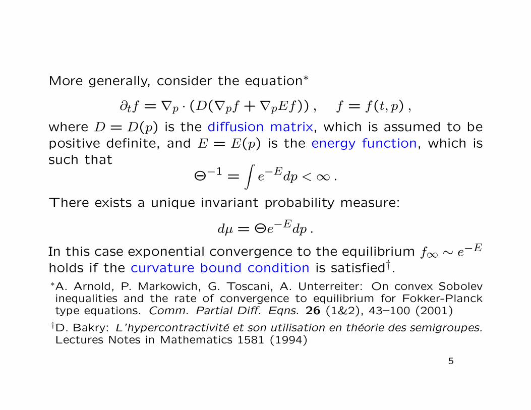
More generally, consider the equation∗

∂tf = ∇p · (D(∇pf +∇pEf)) , f = f(t, p) ,

where D = D(p) is the diffusion matrix, which is assumed to bepositive definite, and E = E(p) is the energy function, which issuch that

Θ−1 =∫e−Edp <∞ .

There exists a unique invariant probability measure:

dµ = Θe−Edp .

In this case exponential convergence to the equilibrium f∞ ∼ e−Eholds if the curvature bound condition is satisfied†.∗A. Arnold, P. Markowich, G. Toscani, A. Unterreiter: On convex Sobolevinequalities and the rate of convergence to equilibrium for Fokker-Plancktype equations. Comm. Partial Diff. Eqns. 26 (1&2), 43–100 (2001)†D. Bakry: L’hypercontractivite et son utilisation en theorie des semigroupes.Lectures Notes in Mathematics 1581 (1994)

5

Sketch of the proof: In terms of h = f/f∞ the equation takes

the form

∂th = ∇ · (D∇h)−D∇E · ∇h ,

or, equivalently,

∂th = ∆Gh+Qh ,

where ∆G denotes the Laplace-Beltrami operator associated to

the Riemannian metric G = D−1 and Q is the vector field

Qh = D∇ logu · ∇h , u =√

detD e−E .

Consider a positive solution h normalized to a probability density:

‖h(t)‖L1(dµ) = 1 .

6

The entropy functional is given by

D[h] =∫RN

h logh dµ ,

and satisfiesd

dtD[h] = −I[h] , where I[h] =

∫RN

D∇h · ∇hh

dµ

is the entropy dissipation functional. Let RicG and ∇G denotethe Ricci tensor and the Levi-Civita connection of G. Bakry andEmery proved that if the curvature bound condition

RicG −∇GQ ≥ γ G , for some γ > 0 ,

is satisfied, then the logarithmic Sobolev inequality

D[h] ≤ (2γ)−1I[h]

holds, for all sufficiently regular probability densities h (not nec-essarily solutions).

7

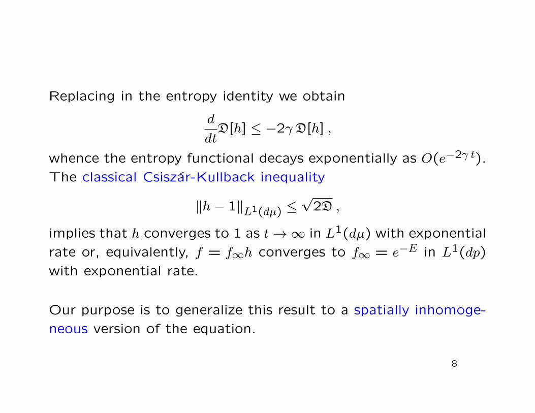
Replacing in the entropy identity we obtain

d

dtD[h] ≤ −2γD[h] ,

whence the entropy functional decays exponentially as O(e−2γ t).

The classical Csiszar-Kullback inequality

‖h− 1‖L1(dµ) ≤√

2D ,

implies that h converges to 1 as t→∞ in L1(dµ) with exponential

rate or, equivalently, f = f∞h converges to f∞ = e−E in L1(dp)

with exponential rate.

Our purpose is to generalize this result to a spatially inhomoge-

neous version of the equation.

8

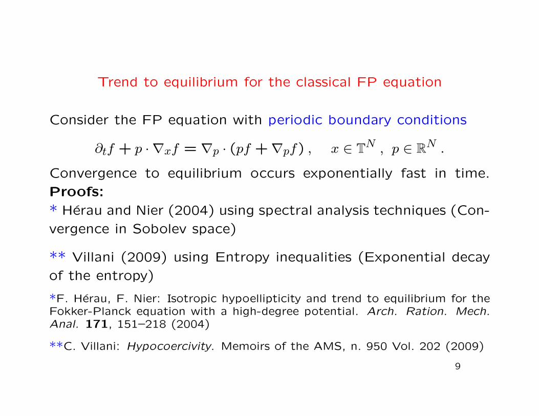
Trend to equilibrium for the classical FP equation

Consider the FP equation with periodic boundary conditions

∂tf + p · ∇xf = ∇p · (pf +∇pf) , x ∈ TN , p ∈ RN .

Convergence to equilibrium occurs exponentially fast in time.

Proofs:

* Herau and Nier (2004) using spectral analysis techniques (Con-

vergence in Sobolev space)

** Villani (2009) using Entropy inequalities (Exponential decay

of the entropy)

*F. Herau, F. Nier: Isotropic hypoellipticity and trend to equilibrium for theFokker-Planck equation with a high-degree potential. Arch. Ration. Mech.Anal. 171, 151–218 (2004)

**C. Villani: Hypocoercivity. Memoirs of the AMS, n. 950 Vol. 202 (2009)

9

Remark: The previous results apply also to the equation in thewhole space (x ∈ RN), with an external confining potential.

We consider the more general equation

∂tf + v(p) · ∇xf = ∇p(D(∇pf + f∇pE)) ,

where D = D(p) is the diffusion matrix and E = E(p) is theenergy function. We also allow for a general velocity field v

in the transport term, the two most interesting cases for theapplications being the classical velocity field

v(p) = p

and the relativistic velocity field

v(p) =p√

1 + |p|2.

10

Setting h = f/e−E, the equation takes the form

∂th+ v(p) · ∇xh = ∆(g)p h+Wh , t > 0 , x ∈ TN , p ∈ RN ,

where ∆(g)p is the Laplace-Beltrami operator associated to the

metric g = D−1 and

Wh = D∇p logu · ∇ph , u =√

detD e−E .

The main result shows that under suitable assumptions on the

functions v,D,E , which take the form of geometric inequalities

involving these quantities, smooth solutions with unit mass con-

verge in time to the equilibrium state h∞ ≡ 1 with exponential

rate of convergence. The proof is carried out using differential

calculus on Riemannian manifolds.

11

Theorem 1 Consider a smooth non-negative initial datum hin,

normalized to a probability density, for the equation

∂th+ v(p) · ∇xh = ∆(g)p h+Wh , t > 0 , x ∈ TN , p ∈ RN ,

Under suitable assumptions (see later) on the metric g, the veloc-

ity field v and the vector field W , there exists a constant C > 0,

depending on suitable norms of hin, and a constant λ > 0, which

can be explicitly computed, such that the entropy functional

D[h] =∫TN×RN

h logh dx dµ

satisfies

D[h](t) ≤ Ce−λt .

12

Example: The relativistic Fokker-Planck equation

For the relativistic kinetic Fokker-Planck equation we have

v(p) =p√

1 + |p|2, D =

I + p⊗ p√1 + |p|2

, E = θ√

1 + |p|2 . (1)

We set the rest mass of the particles and the speed of light equal

to one. The equilibrium state is given by the Juttner distribution

Jθ(p) = Ze−θ√

1+|p|2 , (2)

where Z is a constant (fixed by the mass of the system) and θ

is a positive parameter which, up to a dimensional constant, co-

incides with 1/T , where T is the temperature of the surrounding

bath in which the particles are moving.

13

In terms of h = feE the relativistic Fokker-Planck equation takes

the form

∂th+ v(p) · ∇xh = ∆(g)p h+Wh , t > 0 , x ∈ T3 , p ∈ R3 ,

where ∆(g)p is the Laplace-Beltrami operator associated to the

metric

gij = (D−1)ij = p0(δij −pipj

p20

) , p0 =√

1 + |p|2 .

and

Wh = D∇p logu · ∇ph , u =√

detD e−E =e−θp0

√p0

.

14

Theorem 2 Let 0 ≤ fin be an initial datum of mass M > 0 for

the the relativistic Fokker-Planck equation. Denote by Jθ,M the

Juttner distribution with mass M . Then there exists θ0 > 0 such

that for all θ ≥ θ0 there exists a positive constant λ, depending

on θ, and a positive constant C such that the solution f of the

relativistic Fokker-Planck equation satisfies

‖f − Jθ,M‖L1 ≤ Ce−λt.

Thus exponential convergence to equilibrium occurs for suffi-

ciently small temperatures.

15

Assumptions of the main theorem

Recall that the equation under study is

∂th+ v(p) · ∇xh = ∆ph+Wh , t > 0 , x ∈ TN , p ∈ RN ,

where ∆p = ∆(g)p is the Laplace-Beltrami operator associated to

a Riemannian metric g and W is the vector field W = ∂p logu,

where

u = e−E/√

det g and dµ ∼ e−Edx dp

The Bakry-Emery-Ricci tensor is defined by

Ric = Ric−∇pW∗ = Ric−∇2p logu

16

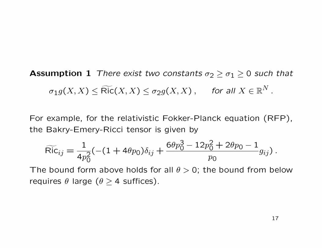
Assumption 1 There exist two constants σ2 ≥ σ1 ≥ 0 such that

σ1g(X,X) ≤ Ric(X,X) ≤ σ2g(X,X) , for all X ∈ RN .

For example, for the relativistic Fokker-Planck equation (RFP),

the Bakry-Emery-Ricci tensor is given by

Ricij =1

4p20

(−(1 + 4θp0)δij +6θp3

0 − 12p20 + 2θp0 − 1

p0gij) .

The bound form above holds for all θ > 0; the bound from below

requires θ large (θ ≥ 4 suffices).

17

Let us define a symmetric bilinear form A on RN × RN by

A(ξ, η) = Aijξiηj , Aij = g(∂pv(i), ∂pv

(j)) , ξ, η ∈ RN .

Assumption 2 We assume that A is positive definite,

A(ξ, ξ) > 0 , for all 0 6= ξ ∈ RN .

For example, for RFP we have

Aij =1

p30

(δij −pipj

p20

)

which is positive definite.

18

Definition 1 We define the Riemannian metric G on TN × RNas

G = Aijdxi ⊗ dxj + gijdp

i ⊗ dpj , (3)

where Aij is the matrix inverse of Aij. Moreover we define thevector field Q ∈ RN as

Q = W − ∂p log√

det(Aij) . (4)

Assumption 3 We assume that there exists a constant γ ≥ 0such that

RicG(Z,Z)−(∇GQ∗)(Z,Z) ≥ γ G(Z,Z) , for all Z ∈ X(TN×RN) ,

where RicG is the Ricci tensor of G and ∇G is the covariantdifferential associated to G.

For RFP, the previous assumption holds for θ large enough.

19

Next let B,C denote the symmetric bilinear forms on RN × RN

given by

B(ξ, η) = Bijξiηi , Bij = g(divp ∂2p v

(i),divp ∂2p v

(j)) ,

C(ξ, η) = Cijξiηj , Cij = ∂2p v

(i) · ∇2pv

(j) ,

Assumption 4 We assume that there exist two constants α, β ≥0 such that

B(ξ, ξ) ≤ αA(ξ, ξ) , C(ξ, ξ) ≤ βA(ξ, ξ) , for all ξ ∈ RN .

This assumption is automatically satisfied if ∇2pv

(i) = 0, e.g. for

the classical Fokker-Planck equation .

20

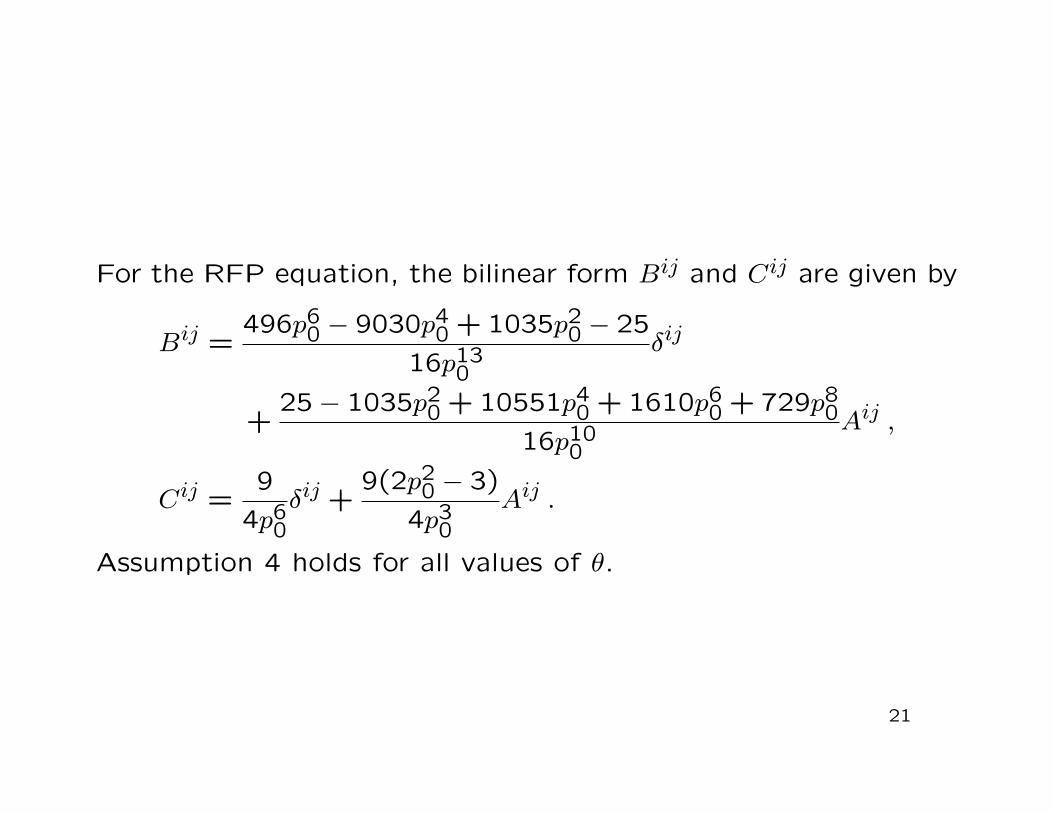
For the RFP equation, the bilinear form Bij and Cij are given by

Bij =496p6

0 − 9030p40 + 1035p2

0 − 25

16p130

δij

+25− 1035p2

0 + 10551p40 + 1610p6

0 + 729p80

16p100

Aij ,

Cij =9

4p60δij +

9(2p20 − 3)

4p30

Aij .

Assumption 4 holds for all values of θ.

21

For the last assumption we define the vectors K(1), . . .K(N) by

K(i)(·) = ∂2p v

(i)(W∗, ·) ,

i.e., componentwise,

K(i)l = (∇2

pv(i))ljW

j .

Let R denote the bilinear form on RN × RN given by

R(ξ, η) = Rijξiηj , Rij = g(K(i),K(j)) .

Assumption 5 We assume that there exists a constant ω > 0

such that

R(ξ, ξ) ≤ ωA(ξ, ξ) , for all ξ ∈ RN . (5)

22

This assumption is automatically satisfied if ∇2pv

(i)(W, ·) = 0,

i.e., when the vector field W lies in the kernel of the Hessian of

v(i), for all i = 1, . . . , N .

For the RFP equation the bilinear form Rij is given by

Rij =(1 + 2θp0)2

16p90

(16(p20 − 1)δij + p3

0(9p40 − 34p2

0 + 25)Aij)

and this verifiesR(ξ, ξ) ≤ ωA(ξ, ξ), for some positive ω, i.e., As-

sumption 5 is satisfied, for all values of θ > 0.

23

Proof of the main theorem

Let h = logh and define

D[h] =∫h h dx dµ

Ipp[h] =∫g(∂ph, ∂ph) dx dµ ,

Ixp[h] =∫g(Axh, ∂ph) dx dµ ,

Ixx[h] =∫g(Axh,Axh) dx dµ ,

where Axf = (∂xif)∂pv(i). Given four constants a, b, c, k > 0, we

define the modified entropy as

E[h] = kD[h] + a Ipp[h] + 2b Ixp[h] + c Ixx[h] .

24

The proof can be divided in three steps

1) Study the time evolution of the modified entropy, by comput-ing the time derivative of D, Ixx, Ixp and Ipp.

2) Prove that the constants a, b, c, k can be chosen so that thefollowing inequalities hold:

(i) D . E, (ii) a Ipp+2b Ixp+c Ixx . Ixx+Ipp, (iii) E . −(Ixx+Ipp).

3) Prove the Logarithmic Sobolev inequality

(iv) D . Ixx + Ipp .

From (iii) − (iv) it follows that E . −D. Moreover by (ii) and(iii) we have E . −(a Ipp + 2b Ixp + c Ixx), so

E . −E ⇒ E = O(e−λ t) .

Finally by (i) we have D = O(e−λ t).

25

Comparision with Villani’s work

The problem of interest here is also covered by Villani’s work

C. Villani: Hypocoercivity. Memoirs of the AMS, n. 950 Vol. 202(2009)

Villani’s work exploits the following form of rewriting the equa-tion:

∂th = (A∗A+B)h ,

for suitable vector fields A,B and is based on the study of thecommutators

[A,B] , [A, [A,B]] , [A, [A, [A,B]]] , . . .

(as in Hormander’s condition for hypoellipticity).

26

However:

1) The use of commutators leads inevitably to very heavy and

sometimes obscure calculations, which, as pointed out by Villani

in his work it might be an indication that a more appropriate

formalism is still to be found. The formalism of differential ge-

ometry helps to clarify the meaning of many long expressions

that have to be controlled in Villani’s work.

2) One has to find a suitable way to decompose the vector fields

A,B and their commutators in order to verify the assumptions of

Villani’s theorem. In the theorem proved here these assumptions

take the form of explicit geometric inequalities on the metric g

and the vector field v,W .

27

Open problems

Open problems that deserve further investigation:

• Generalize the result to the equation with an external con-

fining potential and with time dependent diffusion matrix

• Extend the result to general Riemannian manifolds

• Non-linear problems?

28