troy benn ms thesis

ANALYSIS OF ADSORPTIVE MEDIA TO REMOVE ARSENIC AND CO-OCCURRING

OXYANIONS FROM GROUNDWATER

by

Troy M. Benn

A Thesis Presented in Partial Fulfillment of the Requirements for the Degree

Master of Science

ARIZONA STATE UNIVERSITY

August 2006

ANALYSIS OF ADSORPTIVE MEDIA TO REMOVE ARSENIC AND CO-OCCURRING

OXYANIONS FROM GROUNDWATER

by

Troy M. Benn

has been approved

May 2006

APPROVED:

, Chair

Supervisory Committee ACCEPTED: Department Chair Dean, Division of Graduate Studies

iii

ABSTRACT

In January 2006 the Environmental Protection Agency (EPA) lowered the arsenic maximum contaminant

level (MCL) for drinking water, and a great deal of research has been focused on the arsenic removal

capacity of commercially available adsorptive media. The co-removal of groundwater constituents other

than arsenic has a detrimental effect on the useful longevity of the media. Rapid small-scale column tests

(RSSCTs) were conducted at EPA small system demonstration sites to compare data with the full- or pilot-

scale systems. Additionally, the RSSCTs were used to evaluate the capacity of various adsorptive media to

remove oxyanions of uranium, antimony, phosphorous, and vanadium simultaneously with arsenic. It was

found that RSSCT data can simulate full- and pilot-scale column data. While all adsorptive media tested

showed a capacity to remove phosphorous and vanadium, an iron-enhanced Ion Exchange resin

(ArsenXnp) showed a significant capacity to remove uranium. Only one set of RSSCTs had a significant

amount of antimony (13 ppb) in the source water which could be treated to the 6 ppb MCL for 19,000 bed

volumes by titanium-dioxide media (Dow Absorbsia).

iv

TABLE OF CONTENTS

Page

LIST OF FIGURES.......................................................................................................................................vii

LIST OF TABLES .........................................................................................................................................ix

ACRONYMS AND ABBREVIATIONS........................................................................................................x

Chapter 1: Introduction ...................................................................................................................................1

1.1 Background ........................................................................................................................................1

1.1.1 Arsenic Interaction with Metal (Hydr)Oxide Surfaces.........................................................2

1.1.2 Mass Transport of Ions in Porous Adsorbents......................................................................3

1.1.3 Rapid Small Scale Column Tests for Arsenic Removal by Porous Adsorbents ...................4

1.2 Project Objectives ..............................................................................................................................6

Chapter 2: Methods and Materials ..................................................................................................................9

2.1 Design and Operation of Rapid Small Scale Column Test.................................................................9

2.1.1 RSSCT Apparatus ................................................................................................................9

2.1.2 Adsorbent Media Tested.......................................................................................................9

2.1.3 Preparing RSSCTs for Tests...............................................................................................10

2.1.4 Field Setup for RSSCTs .....................................................................................................11

2.1.5 Laboratory Setup for RSSCTs............................................................................................11

2.1.6 Sample Collection from RSSCTs .......................................................................................12

2.2 Site Descriptions and Water Chemistry ...........................................................................................12

2.3 Analytical Procedures ......................................................................................................................12

Chapter 3: Results and Discussion ................................................................................................................22

3.1 Valley Vista, Arizona (Site1) ...........................................................................................................22

3.1.1 Valley Vista Field RSSCT Results (Site 1F) ......................................................................22

3.1.2 Valley Vista Laboratory RSSCT Results (Site 1L) ............................................................23

3.1.3 Comparison of Field RSSCT, Laboratory RSSCT and Demonstration Scale Results........24

3.2 Rimrock, Arizona Results (Site 2) ...................................................................................................24

3.2.1 Arsenic Removal ................................................................................................................25

v

3.2.2 Removal of Other Oxyanions .............................................................................................25

3.3 Licking Valley School District, Newark, Ohio Results (Site 3).......................................................26

3.3.1 Arsenic Removal Comparison Between RSSCT and Pilot-scale Results...........................26


3.4 Lyman, Nebraska Results (Site 4)....................................................................................................27

3.4.1 Arsenic Removal ................................................................................................................28

3.4.2 Uranium Removal ..............................................................................................................28


3.5 Lake Isabella, California Results (Site 5).........................................................................................29

3.5.1 Arsenic Removal ................................................................................................................29

3.5.2 Uranium Removal ..............................................................................................................30

3.5.4 Summary of Results ...........................................................................................................30

3.6 Reno, Nevada Results (Site 6)..........................................................................................................31

3.6.1 Arsenic Removal ................................................................................................................32

3.6.2 Antimony Removal ............................................................................................................32


3.7 Arsenic Adsorption Density of Media..............................................................................................33

3.8 Layne Christensen RSSCTs (Scottsdale, AZ site water)..................................................................35

3.8.1 Arsenic Removal ................................................................................................................35


3.8.3 Summary of Results ...........................................................................................................36

Chapter 4: Removal of Metals Co-Occurring with Arsenic ..........................................................................56

4.1 Determination of Thomas Fit Parameters.........................................................................................56

4.2 Co-Removal of Antimony (Sb): .......................................................................................................60

4.3 Co-Removal of Uranium (U): ..........................................................................................................60

4.4 Co-Removal of Phosphorous (P) and Vanadium (V):......................................................................62

4.5 Mass of solute removed per media...................................................................................................63

4.5 Discussion ........................................................................................................................................64

vi

Chapter 5: Conclusions .................................................................................................................................73

APPENDIX A ...............................................................................................................................................78

A.1 Dataset for Valley Vista, Arizona Site ............................................................................................79

A.1 Dataset for Valley Vista, Arizona Site (cont.).................................................................................80

A.1 Dataset for Valley Vista, Arizona Site (cont.).................................................................................81

A.2 Dataset for Rimrock, Arizona Site ..................................................................................................81

A.2 Dataset for Rimrock, Arizona Site ..................................................................................................82

A.2 Dataset for Rimrock, Arizona Site (cont.) .......................................................................................83

A.3 Dataset for Licking Valley School District, Ohio Site ....................................................................84

A.3 Dataset for Licking Valley School District, Ohio Site (cont.).........................................................85

A.4 Dataset for Lyman, Nebraska Site...................................................................................................86

A.4 Dataset for Lyman, Nebraska Site (cont.) .......................................................................................87

A.5 Dataset for Lake Isabella, California Site........................................................................................88

A.5 Dataset for Lake Isabella, California Site (cont.) ............................................................................89

A.6 Dataset for Reno, Nevada Site.........................................................................................................90

A.6 Dataset for Reno, Nevada Site (cont.) .............................................................................................91

A.7 Dataset for Layne Christensen Project, Scottsdale, Arizona Site ....................................................92

vii

LIST OF FIGURES

Page

Fig. 1.1. Arsenate (As(V)) Speciation......................................................................................................7

Fig. 1.2. Arsenite (As(III)) Speciation .....................................................................................................7

Fig. 2.1. Illustration of Stand-Alone RSSCT apparatus dimensions (upper) and layout with

column and pump (lower) ...........................................................................................................14

Fig. 2.2. Schematic of packed RSSCT column ......................................................................................15

Fig. 3.1. Valley Vista RSSCT field data for arsenic breakthrough ........................................................37

Fig. 3.3. Lab RSSCT arsenic data for Valley vista, AZ .........................................................................38

Fig. 3.4. A comparison of RSSCT lab data versus RSSCT field data for Valley Vista, AZ ..................39

Fig. 3.5. Comparison of Lab/Field RSSCT versus Full-scale system (AAFS50)...................................40

Fig. 3.6. RSSCT arsenic data for Rimrock, AZ......................................................................................40

Fig. 3.7. RSSCT arsenic-competing ions (V,P,Si,Fe) data for Rimrock, AZ.........................................41

Fig. 3.8. RSSCT Results for Licking Valley School District, Newark, OH...........................................42

Fig. 3.9. Comparison of RSSCTs with Pilot-scale Results for Licking Valley School District,

Newark, OH.................................................................................................................................42

Fig. 3.10. Oxyanion (P, Si, Fe) Breakthrough Curves for Licking Valley School District,

Newark, OH.................................................................................................................................43

Fig. 3.11. RSSCT arsenic data for Lyman, NE ......................................................................................44

Fig. 3.12. Breakthrough data comparison of titanium dioxide media (GTO and MetsorbG)

columns packed using Reynold-Schmidt numbers of 1000 and 2000 .........................................45

Fig. 3.13. Isotherm experiments for media used in Lyman, NE water...................................................46

Fig. 3.14. RSSCT oxyanion (U, V, Fe, Mn) breakthrough data for Lyman, NE....................................47

Fig. 3.15. Lake Isabella RSSCT arsenic data which simulated an EBCT of 5.3 min except **

which required a simulated EBCT of 2.5 min .............................................................................48

Fig. 3.16. Comparison of titanium dioxide (GTO and MetsorbG) media RSSCTs conducted with

Reynold-Schmidt numbers of 1000 or 2000 in Lake Isabella RSSCTS......................................48

viii

Fig. 3.17. Lake Isabella isotherm experiments.......................................................................................49

Fig. 3.18. Lake Isabella RSSCT breakthrough data for uranium. EBCTs were simulated at 5.3

min except ** which required a simulated EBCT of 2.5 min......................................................49

Fig. 3.19. Comparison of titanium dioxide media (GTO and MetsorbG) for Lake Isabella

RSSCT uranium breakthrough data. EBCT was simulated at 2.5 min ........................................50

Fig. 3.20. Arsenic breakthrough data from Reno, NV RSSCTs. EBCTs were simulated at 3 min. .......50

Fig. 3.21. Reno isotherm experiments....................................................................................................51

Fig. 3.22. Comparison of GFH columns packed at 3 & 6.2 min. EBCTs for Reno RSSCTs.................51

Fig. 3.23. Antimony breakthrough data for Reno RSSCTs with a simulated EBCT of 3 min. ..............52

Fig. 3.24. Oxyanion breakthrough data for Reno RSSCTs with a simulated EBCT of 3 min. ..............53

Fig. 3.25. Arsenic breakthrough curves for Layne Christensen RSSCTs with iron-based media ..........53

Fig. 3.26. Arsenic breakthrough curves for Layne Christensen RSSCTs with titanium-based

media ...........................................................................................................................................54

Fig. 3.27. Batch isotherm data for the iron-based media (and Melstream RS-AF) ................................54

Fig. 3.28. Batch isotherm data for the titanium based media .................................................................55

Fig. 3.29. Phosphorous and vanadium breakthrough curves for the Layne Christensen RSSCTs .........55

Fig. 4.1. Thomas Fit Estimation of Experimental Data..........................................................................66

Fig. 4.2. Effect of Adjusting Thomas Rate Constant, k..........................................................................67

Fig. 4.3. Effect of Adjusting the Maximum Solid Phase Concentration, q0 ...........................................67

Fig. 4.4. Examples of solute breakthrough abnormalities from Lyman RSSCTs. Data points

represent observed data while the solid line represents the Thomas fit. ......................................68

Fig. 4.5. Common examples of Thomas equation fit to various adsorbate breakthrough data...............69

Fig. 4.6 Arsenic Removal Performance from Reno RSSCTs.................................................................70

Fig. 4.7. Comparative Arsenic Removal for Lake Isabella RSSCTs......................................................70

Fig. 4.8. Comparative Arsenic Removal for Lyman RSSCTs................................................................71

Fig. 4.9. Normalized As, P, and V breakthrough curves for E33 media with Lyman, NE water...........71

Fig. 4.10. Example of mass of solute removed per mass of media calculation......................................72

ix

LIST OF TABLES

Page

Table 1.1. RSSCT Scaling Equations.......................................................................................................8

Table 2.1. Description of Commercial Arsenic Adsorption Media Used in RSSCTs............................16

Table 2.2. Full-scale design conditions used to scale RSSCTs ..............................................................17

Table 2.3. Design parameters used for RSSCTs ....................................................................................18

Table 2.4. Summary of Sampling Frequency and Analysis ...................................................................19

Table 2.5. Summary of site locations, date for water collection, and key water quality

parameters of influent RSSCT water...........................................................................................20

Table 2.6. Analytical Methods, Sample Volumes, Containers, Preservations, and Holding Times.......21

Table 3.1 Comparison of bed volumes treated before exceeding MCLs for co-occurring

contaminants, Lyman, NE ...........................................................................................................29


contaminants, Lake Isabella, CA.................................................................................................31


contaminants, Reno, NV..............................................................................................................33

Table 3.4 Summary of arsenic adsorption capacities .............................................................................34

Table 4.1. Thomas fit parameters k and q0 for various solutes (As, U, Sb, P, V, Mn) and

adsorptive media..........................................................................................................................58

Table 4.1. (cont.) ....................................................................................................................................59

Table 4.2. Thomas Fit Parameters for Sb (Reno RSSCT)......................................................................60

Table 4.3. Thomas Fit parameters and bed volumes treated to the MCL for U removal in Lake

Isabella and Lyman RSSCTs.......................................................................................................61

Table 4.4. Thomas Fit parameters for V removal in Layne Christensen and Lyman RSSCTs ..............62

Table 4.5. Bed Volumes Treated to 50% of Influent Concentration of Phosphorous ............................63

Table 4.6. Solute Mass Removal Densities for each media calculated at full As breakthrough ............64

x

ACRONYMS AND ABBREVIATIONS Al Aluminum

As Arsenic

As(III) Arsenite

As(V) Arsenate

ASU Arizona State University (Tempe, AZ)

AZ Arizona

Ca Calcium

CA California

Cl- Chloride

dp Media particle diameter

E33 Granular ferric (hydr)oxide (product of Severn Trent Services)

EBCT Empty bed contact time

Fe Iron

ICP-MS Ion coupled plasma mass spectrometery

GFH Granular ferric hydroxide (product of US Filter)

GTO Granular titanium oxide (product of DOW Chemical)

MCL Maximum contaminant limit

MDL Minimum detection limit

Mn Manganese

xi

NE Nebraska

NO3- Nitrate

NV Nevada

OH Ohio

P Phosphorous

QAPP Quality assurance project plan

RSSCT Rapid small scale column test

Sb Antinomy

SO42- Sulfate

TO Task order

TOC Total organic carbon

U Uranium

USEPA United States Environmental Protection Agency

V Vanadium

As0 Initial arsenate concentration (μg/L)

As Final arsenate concentration (μg/L)

Asb Arsenate concentration in the bulk solution (μg/L)

xii

Ass Arsenate concentration at solid/liquid interface

K Freundlich coefficient

n Freundlich coefficient

qavg Average adsorptive capacity (μg/mg)

q adsorptive capacity (μg/mg)

qm Maximum solid phase concentration (μg/mg)

CAs Equilibrium concentration between solid and liquid phase (μg/mg)

r Radial coordinate from the center of the particle

Rp Radius of Particle (cm)

dp Particle diameter(cm)

Vr Volume of the reactor (L)

v Interstitial velocity (cm/sec)

∈ Void fraction

m mass of the media in the DCBR column

t time

ρb Apparent bulk density (g/L)

Bi Biot number =Q**DAs*R*K

as

0pf

ρ

Sh Sherwood Number =mol

fp

DK*R*2

Sc Schmidt Number =molD*ρ

μ

St Stanton Number =p

f

R**)1(*K

∈

∈− τ

Re Reynolds Number =μρ v**R*2 p

Kf External Mass Transfer Coefficient (cm/sec)

xiii

Dp Pore diffusion coefficient (cm2/sec)

Ds Surface diffusion coefficient (cm2/sec)

DL Free liquid diffusivity (cm2/sec)

μ Solution viscosity

Chapter 1: Introduction The lowering of the maximum contaminant level (MCL) for arsenic in drinking water from 50 ppb to 10

ppb by the United States Environmental Protection Agency (USEPA) in January of 2006 has fueled the

research of efficient cost-effective treatment technologies. Adsorptive media have long been known to

effectively treat water contaminated with arsenic. Rapid small-scale column tests (RSSCTs) were utilized

to accomplish specific goals. First, the RSSCTs were conducted with water samples collected from EPA

test sites to compare arsenic breakthrough data to full-scale column operations. The RSSCTs were scaled

down using an approach initially developed for organics removal by activated carbon and recently verified

for arsenic removal by porous metal (hydr)oxides (Badruzzaman et al. 2004; Crittenden et al. 1986;

Crittenden et al. 1987; Westerhoff et al. 2005). This down-scaling validates the use of RSSCTs to produce

data that is comparable to that of a full-scale test in a fraction of the time. Second, the data collected from

the RSSCTs will be analyzed for metals that are simultaneously removed with arsenic by the adsorptive

media. This data will give insight to the amount of constituents that adsorb to the media which might be

detrimentally affecting the arsenic removal capacity. Additionally, there are objectives for each set of

RSSCTs that were conducted for specific EPA research sites. These objectives will be clarified in their

appropriate sections.

1.1 Background

Battelle is currently contracted by EPA, under Task Order (TO) # 019, Contract 68-C-00-185, to conduct

12 full-scale, long-term, on-site demonstrations of arsenic removal technologies applicable to small

systems. This project is part of an EPA initiative to assist small community water systems (< 10,000

customers) in complying with the new arsenic standard. Nine of the 12 demonstration projects involve the

adsorptive media arsenic removal technology. This technology was selected because of advantages for

treating small water flows. The selection of the media for these projects has been based upon the state-of-

the-art procedures for evaluating adsorptive media performance consisting of long-term pilot plant studies.

Because of the length of time required for evaluating the capacities of many of the new adsorptive media

products (usually 9 to 12 months), the cost of the studies is substantial. To reduce the cost and to reduce

the time to evaluate the performance of these media products, several preliminary research studies have

2

been recently conducted using the rapid small-scale column tests method that was developed years ago for

evaluating the performance of granular activated carbon. The results of these studies have shown that the

RSSCT method, that usually requires only three to four weeks of testing, has the potential to predict the

performance of full-scale system performance. If this proves to be true, the method would provide the

industry with a lower cost method to develop performance data necessary for full-scale design of arsenic

removal adsorptive media processes. To verify the usefulness of this short-term predictive method, side-

by-side tests (RSSCT verse full scale system) are required.

1.1.1 Arsenic Interaction with Metal (Hydr)Oxide Surfaces

Arsenate (H3AsO4, H2AsO4-, HAsO4

2-, or AsO43-) is the dominant form in oxygenated waters, present in

anionic form over the pH range of 5 to 12 (Figure 1.1). Over the pH range of most groundwaters, arsenate

is present as both H2AsO4- and HAsO4

2-. Arsenite occurs under reducing conditions (Eh<0 V at pH ~7) and

is present in a nonionic form (H3AsO3) below pH ~9.2 (McNeill and Edwards 1997). Chlorine,

permanganate, or ozone readily oxidizes arsenite to arsenate, with less effective oxidation by

monochloramine, chlorine dioxide, or oxygen.

Arsenic (i.e., arsenate and arsenite) can associate with iron surfaces either by forming inner-sphere

or outer-sphere complexes (Goldberg and Johnston 2001; Raven et al. 1998; Wilkie and Hering 1996).

Surface chemistry is important in arsenic removal by metal oxides. The surfaces of metal oxides are

collections of unfilled metal-oxygen bonds that hydrate in water. Electrostatic attraction of anionic species

is favored onto positively charge surface sites. At the pH zero point of charge (pHZPC), an equal number of

positive and negatively charged surface sites exist, and proportionally more positive surface sites at pH

levels below the pHZPC. Therefore, the pHZPC is one indicator for the potential to remove anionic arsenic

species. Iron (hydr)oxides have pKa1 and pKa2 values of ~7.3 and 8.9, respectively, resulting in a pHZPC on

the order of 8.1. Anionic arsenic species are generally removed better than non-ionic arsenic species by

most adsorbents.

3

Coulombic forces favor association of anionic arsenate with positive surface sites (e.g., MeOH2+).

In addition to this electrostatic bonding between arsenic species and mineral surfaces, arsenic will also

form covalent bonds with some surfaces. These include monomolecular monodentate and monomolecular

bidentate bonds. Whereas electrostatic bonds form rapidly (seconds) and depend on the charge difference

between the arsenic and the surface, covalent bonds depend on their respective molecular structure and

form less rapidly. Covalent bonds are stronger (i.e., irreversible) than electrostatic attractions. As covalent

bonds form, surface sites can become available for electrostatic bonding again. The kinetics of bond

formation may affect the optimal contact time required for a specific media in a column operation.

Silica can be a major anion that exerts significant impact in arsenate removal by porous adsorbents. A few

batch and column studies have been documented that silica reduces arsenic adsorption capacity of ferric

oxides/hydroxides and activated alumina (Meng et al. 2000; Meng et al. 2002). Several mechanisms have

been documented to describe the role of silica in iron-silica and iron-arsenic-silica systems, such as (a)

adsorption of silica might change the surface properties of adsorbents by lowering the iso-electric point

(pHzpc), (b) silica might compete for arsenic adsorption sites, (c) polymerization of silica might accelerate

silica sorption and lower the available surface sites for arsenic adsorption, and (d) the chemical reaction of

silica with divalent cations such as calcium, magnesium and barium might form precipitates. Other anions,

and cations, can affect surface charge and thus impact arsenic removal by metal (hydr)oxide adsorbent

media.

1.1.2 Mass Transport of Ions in Porous Adsorbents

Iron, aluminum, titanium, zirconium, and other metal-oxide based adsorbents have been commercialized

over the past decade specifically to remove arsenic from water. Most of these have fairly high surface

areas (>100 m2/g) and have a continuum of micro- and macro-pores (Badruzzaman et al. 2004). Mass

transport of arsenic from solution onto and into these porous adsorbents has been described by film

diffusion and intraparticle surface or pore diffusion coefficients (Badruzzaman et al. 2004; Lin and Wu

2001). Despite the formation of strong bonds between arsenic and the metal oxide, surface diffusion is still

possible (Axe and Trivedi 2002). However, intraparticle transport is probably a combination of surface and

pore diffusion mechanisms.

4

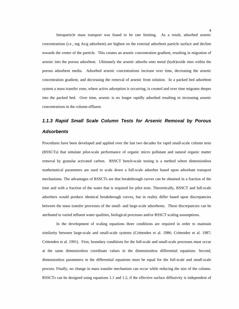
Intraparticle mass transport was found to be rate limiting. As a result, adsorbed arsenic

concentrations (i.e., mg As/g adsorbent) are highest on the external adsorbent particle surface and decline

towards the center of the particle. This creates an arsenic concentration gradient, resulting in migration of

arsenic into the porous adsorbent. Ultimately the arsenic adsorbs onto metal (hydr)oxide sites within the

porous adsorbent media. Adsorbed arsenic concentrations increase over time, decreasing the arsenic

concentration gradient, and decreasing the removal of arsenic from solution. In a packed bed adsorbent

system a mass transfer zone, where active adsorption is occurring, is created and over time migrates deeper

into the packed bed. Over time, arsenic is no longer rapidly adsorbed resulting in increasing arsenic

concentrations in the column effluent.

1.1.3 Rapid Small Scale Column Tests for Arsenic Removal by Porous

Adsorbents

Procedures have been developed and applied over the last two decades for rapid small-scale column tests

(RSSCTs) that simulate pilot-scale performance of organic micro pollutant and natural organic matter

removal by granular activated carbon. RSSCT bench-scale testing is a method where dimensionless

mathematical parameters are used to scale down a full-scale adsorber based upon adsorbate transport

mechanisms. The advantages of RSSCTs are that breakthrough curves can be obtained in a fraction of the

time and with a fraction of the water that is required for pilot tests. Theoretically, RSSCT and full-scale

adsorbers would produce identical breakthrough curves, but in reality differ based upon discrepancies

between the mass transfer processes of the small- and large-scale adsorbents. These discrepancies can be

attributed to varied influent water qualities, biological processes and/or RSSCT scaling assumptions.

In the development of scaling equations three conditions are required in order to maintain

similarity between large-scale and small-scale systems (Crittenden et al. 1986; Crittenden et al. 1987;

Crittenden et al. 1991). First, boundary conditions for the full-scale and small-scale processes must occur

at the same dimensionless coordinate values in the dimensionless differential equations. Second,

dimensionless parameters in the differential equations must be equal for the full-scale and small-scale

process. Finally, no change in mass transfer mechanism can occur while reducing the size of the column.

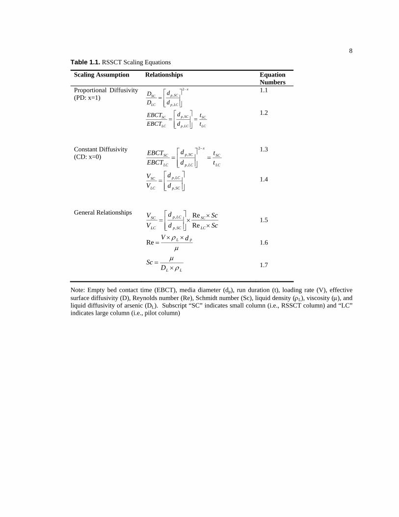
RSSCTs can be designed using equations 1.1 and 1.2, if the effective surface diffusivity is independent of

5

particle size and is therefore identical between the full-scale and RSSCT columns (Table 1.1). If the

surface diffusivities are not identical between the full-scale and RSSCT columns, perfect similarity can not

be guaranteed. However, if it is assumed that surface diffusivity is linearly proportional to the particle

radius and that surface diffusion is the controlling mechanism, an RSSCT can be designed using equations

1.3 and 1.4 that would produce an RSSCT that would perform very similar to the full-scale adsorber. The

Reynolds number is a dimensionless ratio of the inertial forces over the viscous forces in a fluid and the

Schmidt number is a dimensionless ratio of the diffusion of momentum over the diffusion of mass. The

product of the Reynolds number and the Schmidt number can be used to determine the minimum Reynolds

number for the RSSCT such that the effects of dispersion are not important. Dispersion is not important if

the product of the Reynolds number and the Schmidt number is in the mechanical dispersion region from

200,000-200. Equations 1.5 through 1.7 are used to reduce loading rates in the small column and

minimize potential for bed compaction, while maintaining a minimum Reynolds-Schmidt product.

Both proportional and constant diffusivity scaling relationships have recently been applied for

arsenic removal by porous metal (hydr)oxide adsorbents [Westerhoff, 2005 #511; Thomson, 2003 #549;

Sperlich, 2005 #548; Badruzzaman, 2004 #513]. Each research group appears to make different

assumptions and scale to different types of larger scale loading rates and other design parameters. Based

upon the work of Westerhoff, et. al., where multiple comparisons between pilot-scale performance and

RSSCT arsenic breakthrough curves, proportional diffusivity scaling equations appear to accurately mimic

larger scale performance without leading to excessive pressure development within the RSSCTs, as is the

case with constant diffusivity based RSSCTs. So, for both performance and operational issues,

proportional diffusivity scaling relationships were used in this study.

The size of the RSSCTs are based upon the scaling approach (constant or proportional diffusivity)

and the ratio of as-received adsorbent media and the size of media in the RSSCT. Selecting smaller media

sizes for the RSSCTs would decrease the volume of water and duration of the test. However, smaller

media increases the pressure drop across the column (i.e., headloss). Excessive pressure accumulation can

compress “softer” materials and lead to failure of the RSSCT. In previous work 100x140 and 140x170

mesh sizes performed well for most media (Westerhoff et al. 2005). Another assumption for the use of

RSSCTs is that the media is homogeneous. Crushing the media therefore retains the same adsorption

6

mechanisms as the full-scale media. This assumption is valid for most of the commercial metal

(hydr)oxide media.

1.2 Project Objectives

The aim of this thesis is to investigate the efficiency of adsorption technologies to treat arsenic and other

heavy metal contamination of groundwater sources. Specifically, objectives were to:

• Conduct RSSCTs on groundwater samples from multiple EPA small distribution system treatment

demonstration sites.

• Validate the use of RSSCTs to predict full- or pilot-scale arsenic breakthrough data.

• Evaluate commercially available adsorptive media for simultaneous removal of arsenic with

uranium or antimony.

• Investigate the effects on media performance of the simultaneous removal of various oxyanions

with arsenic.

7

Fig. 1.1. Arsenate (As(V)) Speciation

Fig. 1.2. Arsenite (As(III)) Speciation

H3AsO4 AsO43-H2AsO4

- HAsO42-

Perc

enta

ge T

otal

Con

cent

ratio

n

pH

H2AsO3-

HAsO32-AsO3

3-

H3AsO3

Perc

enta

ge T

otal

Con

cent

ratio

n

pH

8

Table 1.1. RSSCT Scaling Equations

Scaling Assumption Relationships Equation Numbers

Proportional Diffusivity (PD: x=1)

LC

SC

LCp

SCp

LC

SC

x

LCp

SCp

LC

SC

tt

dd

EBCTEBCT

dd

DD

=⎥⎥⎦

⎤

⎢⎢⎣

⎡=

⎥⎥⎦

⎤

⎢⎢⎣

⎡=

−

,

,

2

,

,

1.1 1.2

Constant Diffusivity (CD: x=0)

⎥⎥⎦

⎤

⎢⎢⎣

⎡=

=⎥⎥⎦

⎤

⎢⎢⎣

⎡=

−

SCp

LCp

LC

SC

LC

SC

x

LCp

SCp

LC

SC

dd

VV

tt

dd

EBCTEBCT

,

,

2

,

,

1.3 1.4

General Relationships

LL

pL

LC

SC

SCp

LCp

LC

SC

DSc

dV

ScSc

dd

VV

ρμμρ

×=

××=

××

×⎥⎥⎦

⎤

⎢⎢⎣

⎡=

Re

ReRe

,

,

1.5 1.6 1.7

Note: Empty bed contact time (EBCT), media diameter (dp), run duration (t), loading rate (V), effective surface diffusivity (D), Reynolds number (Re), Schmidt number (Sc), liquid density (ρL), viscosity (μ), and liquid diffusivity of arsenic (DL). Subscript “SC” indicates small column (i.e., RSSCT column) and “LC” indicates large column (i.e., pilot column)

9

Chapter 2: Methods and Materials This section discusses the materials and methods used for designing and operating the RSSCTs in the field

and laboratory to evaluate arsenic removal by commercially available media. Section 2.1 describes the

design and operation of the RSSCTs. Section 2.2 describes the sites and influent water chemistry of the

groundwaters used in this study. Section 2.3 discusses pertinent analytical procedures.

2.1 Design and Operation of Rapid Small Scale Column Test

2.1.1 RSSCT Apparatus

Stand-alone RSSCT apparatus were designed and constructed to support one pump and packed adsorbent

bed column. Figure 2.1 illustrates the apparatus. Laboratory columns (Ace Glass, Vineland, NJ) were 1.1

cm diameter glass columns approximately 30.5 cm in length with Teflon end caps. Teflon tubing (3.2 mm)

was used. Piston pumps (QG150, (FMI Inc. Syosset, NY)) with stainless steel or ceramic pump heads

(Q2CSC, FMI Inc. Syosset, NY)) were used. Glass wool was packed into the bottom of the column to

support the adsorbent media. Borosilicate glass beads (5-mm diameter; VWR) were placed at the top the

glass wool to disperse the flow. Figure 2.2 is a schematic of a packed RSSCT column.

2.1.2 Adsorbent Media Tested

Depending upon the site, different adsorbent media were tested. Table 2.1 provides details on the six

adsorbent media used in this study. As-received media from the manufacturer was crushed by mortar and

pestle. Crushed media was sieved using US standard meshes (stainless steel) to obtain a 100x140 mesh

fraction. The media was wet sieved using distilled water until fines no longer migrated out of the 140 mesh

sieve. 100x140 sieved media was transferred to Nalgene bottles containing distilled water and stored until

use for preparing RSSCTs.

An assumption for the use of RSSCTs is that the media is homogeneous. Crushing the media

therefore retains the same adsorption mechanisms as the full-scale media. This assumption is valid for

most of the commercial metal (hydr)oxide media. This assumption may not be valid for ArsenXnp which

10

is an iron-impregnated ion exchange resin. While the resin is porous, recent work suggests that the

concentration of iron is greater near the exterior surface of the bead than at the center of the bead. Thus,

crushing would “normalize” the iron content. It is possible that a higher iron content near the exterior

surface could create a more favorable adsorbed arsenic concentration gradient, and hence better arsenic

removal in the packed bed than observed in the RSSCT.

2.1.3 Preparing RSSCTs for Tests

RSSCT columns were packed using washed and sieved 100 x 140 mesh adsorptive material. Glass beads

and glass wool were placed in the bottom of the column. The amount of material packed into each column

was determined through use of proportional diffusivity scaling equations. In all cases, the RSSCT bed

depth (i.e., RSSCT bed volume) was the critical parameter in preparing the RSSCT columns. To prevent

entrainment of air during column preparation, media was transferred to the RSSCT column while it was

filled with water. After transferring media, the column was backwashed until the effluent was visibly clear

of fine material. The backwashing was then ceased and, to compress the media, the exterior of the glass

column was gently tapped while the media particles settled. Additional media was added, and backwashed,

until the precise desired bed depth was achieved. The mass of the media added to the column can be

estimated from the bulk density and the bed volume of the packed bed. Additionally, the media can be

carefully extracted after completion of the test to measure the total mass. Glass wool and glass beads were

placed on top of the column, and the top Teflon end-cap attached.

The flowrate of the pumps was calibrated prior to attaching the columns. After connecting the

pump to the column, distilled water was passed through for approximately 15 minutes to double check the

flowrate as well as to allow additional settlement of the media bed. The RSSCT columns were then stored

full of distilled water until use. Valves on the top and bottom end-caps were tightly closed to prevent

drainage during storage or transport of the RSSCTs. If air bubbles were observed in the packed media bed

at any time throughout the preparation process, the packing procedure was repeated to remove this air.

Tables 2.2 and 2.3 summarize the key design and operational parameters from the full-scale

system and RSSCT for each media and each site. In most cases a Reynold-Schmidt product of 2000 was

11

used. In select tests with E33 this parameter was adjusted to a value of 1000 for comparison. For titanium

dioxide based media (MetsorbG and Adsorbsia GTO) it was necessary to use a value of 1000 to minimize

bed compaction. In addition with this titanium dioxide based media, in some cases full-scale EBCTs had to

be reduced in the scaling equations in order to decrease the bed depth of the RSSCTs in order to minimize

pressure accumulation and bed compaction. Only data for RSSCTs that operated successfully are shown.

Operational problems associated to pressure accumulation only existed with titanium dioxide based media,

and several unsuccessfully operated columns are not shown.

2.1.4 Field Setup for RSSCTs

Two tests were conducted in the field (Valley Vista, AZ and Licking Valley School District, OH). Valley

Vista, AZ has a demonstration scale arsenic treatment system containing AAFS-50 packed media. Four

RSSCTs were housed in a weatherproof garden storage shed. Water was supplied to the RSSCTs from a

50-gallon Nalgene container that was wrapped to prevent larger thermal variations or algae growth. The

50-gallon container was filled approximately every three days with influent groundwater, which was

filtered (in-line 10 μm glass fiber filter). Effluent from the RSSCTs was discharged to an on-site holding

tank. Licking Valley School District, OH is the site of a Battelle pilot plant. RSSCTs were plumbed into a

water supply port after the solid phase oxidant which removed iron and some of the influent arsenic; this

port supplied water continuously (no on-site influent holding tank). An in-line filter (10 μm glass fiber

filter) was installed prior to the RSSCT. The RSSCT effluent was discharged to the sewer.

2.1.5 Laboratory Setup for RSSCTs

Most of the RSSCTs were conducted in the laboratory (18 oC). Groundwater collected in the field was

filtered (in-line 10 μm glass fiber filter) as it was pumped from the wellsite. Water was filtered (in-line 10

μm glass fiber filter) in the field and collected in HDPE containment bags (i.e., drum liners) placed in 55-

gallon drums; double-lined containment bags were used. The bags were sealed, drums securely closed, and

shipped via truck to ASU laboratories. In the laboratory, water was supplied directly to the RSSCT from

12

the containment bags or a large common influent tank (330 gallon Nalgene tank). RSSCT effluent was

discharged to the sewer.

2.1.6 Sample Collection from RSSCTs

Water samples were collected from the RSSCT influent source water (1 sampling point) and effluent from

each RSSCT over the duration of the RSSCT run. Sampling location, frequency, collection bottle type, and

parameters analyzed are presented in Table 2.4.

2.2 Site Descriptions and Water Chemistry

Table 2.5 includes the location and date from which groundwater was collected for this study. Table 2.5

also includes a description of the key water quality parameters for the water based upon an average of the

RSSCT influent samples collected over the course of each test.

2.3 Analytical Procedures

Table 2.6 also summarizes the analytical methods. Samples for pH and temperature were taken in clean

plastic wide-mouth containers. The containers were rinsed three times with sample water, filled, and pH

and temperature measured immediately. Samples for alkalinity, fluoride, sulfate, orthophosphate, and silica

were collected in a single 1 liter Nalgene-plastic bottle. No filtration or preservation was applied. Samples

were immediately stored in the dark at a cold temperature. Samples for TOC were collected in a 40-mL

glass vials. No filtration was applied. Samples were preserved using acid, to pH 4, using concentrated

hydrochloric acid (HCl). Samples were immediately stored in the dark at a cold temperature. Samples for

metals analysis (As, Fe, Al, Mn, V, Ca) were collected in 60-mL Nalgene-plastic bottles. No filtration was

applied. Samples were acidified to pH<2 with Ultrex high-purity nitric acid (HNO3). Samples were

immediately stored in the dark at a cold temperature.

Samples for arsenic speciation were collected in a 60-mL Nalgene-plastic bottle. The arsenic field

speciation method uses an anion exchange resin column to separate the soluble arsenic species, As(V) and

As(III). A 250-mL bottle (identified as bottle A) was used to contain an unfiltered sample, which is

13

analyzed to determine the total arsenic concentration (both soluble and particulate). The soluble portion of

the sample was obtained by passing the unfiltered sample through 0.45-µm screw-on disc filters to remove

any particulate arsenic and collecting the filtrate in a 125-mL bottle (identified as bottle B). Bottle B

contained 0.05% (volume/volume) ultra-pure sulfuric acid to acidify the sample to about pH 2. At this pH,

As(III) is completely protonated as H3AsO3, and As(V) is present in both ionic (i.e., H2AsO4–) and

protonated forms (i.e., H3AsO4). A portion of the acidified sample in bottle B was run through the resin

column. The resin retains As(V) and allows As(III) (i.e., H3AsO3) to pass through the column. (Note that

the resin will retain only H2AsO4– and that H3AsO4, when passing though the column, will be ionized to

H2AsO4– due to elevated pH values in the column caused by the buffer capacity of acetate exchanged from

the resin.) The eluate from the column was collected in another 125-mL bottle (identified as bottle C).

Samples in bottles A, B, and C are analyzed for total arsenic. As(III) concentration is the total arsenic

concentration of the resin-treated sample in bottle C. The As(V) concentration is calculated by subtracting

As(III) from the total soluble arsenic concentration of the sample in bottle B.

Arsenic speciation kits were prepared in batches at ASU laboratories according to the procedures

described elsewhere. A batch of 50 speciation kits were prepared using one kilogram of Dowex 1-X8, 50-

to 100-mesh chloride-form resin. All chemicals used for preparing the kits were of analytical grade or

higher. Each arsenic speciation kit contained the following items:

• One anion exchange resin column

• One 250-mL bottle (bottle A)

• Two 125-mL bottles (bottles B and C)

• One 400-mL disposable beaker

• One 60-mL disposable syringe

• Several 0.45-µm syringe-adapted disc filters.

14

Fig. 2.1. Illustration of Stand-Alone RSSCT apparatus dimensions (upper) and layout with column and pump (lower)

15

Fig. 2.2. Schematic of packed RSSCT column

O-Ring Teflon End Cap

Glass Beads Glass Wool

Sieved

Adsorbent Media

Glass Wool

Glass Beads

1.1 x 30.5 cm Glass column

Direction of flow

Teflon End Cap O-Ring

16

Table 2.1. Description of Commercial Arsenic Adsorption Media Used in RSSCTs

Media Product

Identifier

Supplier Material Property Full-scale Media Diameter (mm)

Surface Area (m2/g)

E33 Severn Trent Iron oxide 1.16 133 GFH US Filter Iron hydroxide 1.16 259 AA-FS50 Alcan/Kinetico Iron modified activated

alumina 0.85 267

MetsorbG Graver/Hydroglobe Titanium dioxide 0.68 ~125 Adsorbsia GTO

DOW Chemical Titanium dioxide 0.68 70

ArsenXnp Purolite/Solmetex Hybrid ion exchange resin containing iron impregnated on a strong base anion exchange resin

0.75 82

ARM 200 Englehard Iron oxide 1.06 -

17

Table 2.2. Full-scale design conditions used to scale RSSCTs

Site ID Site Location Adsorbent Media Full-scale Design ConditionsDescription Media Diam Loading Rate EBCT Re-Sc Vessel Diam Bed Depth

(mm) (m/h) (min) (cm) (cm)Site 1F Valley Vista, AZ AAFS50 0.85 12.8 4.5 12085 91 183

(field tests) GFH 1.16 12.8 4.5 16500 91 183E33 1.16 12.8 4.5 16500 91 183

AAFS50 0.85 12.8 4.5 12085 91 183

Site 1L Valley Vista, AZ GFH 1.16 12.8 4.5 16500 91 183(lab tests) E33 1.16 12.8 4.5 16500 91 183

AAFS50 0.85 15.6 4.5 14700 91 183

Site 2 Rim Rock, AZ GFH 1.16 15.6 4.5 20059 91 183E33 1.16 15.6 4.5 20059 91 183

AAFS50 0.85 3.7 5.0 3489 5 31

Site 3 Licking Valley GFH 1.16 3.7 5.0 4761 5 31School District, OH E33 1.16 3.7 5.0 4761 5 31

ArsenXnp 0.75 3.7 5.0 3078 5 31ArsenXnp 0.75 17.0 3.0 14175 244 85

Site 4 Lyman, NE E33 1.16 17.0 3.0 21924 244 85DOW Adsorbsia GTO 0.67 17.0 3.0 12663 244 85

MetsorbG 0.67 17.0 3.0 12663 244 85DOW Adsorbsia GTO 0.67 17.0 3.0 12663 244 85

MetsorbG 0.67 17.0 3.0 12663 244 85E33 1.16 9.65 5.3 12435 106.7 152

Site 5 Lake Isabella, CA GFH 1.16 9.65 5.3 12435 106.7 152ArsenXnp 0.75 9.7 5.3 8040 107 152

DOW Adsorbsia GTO 0.67 9.65 2.5 7182 106.7 152DOW Adsorbsia GTO 0.67 9.65 2.5 7182 106.7 152

MetsorbG 0.67 9.65 2.5 7182 106.7 152ARM 200 1.06 9.97 3.0 11745 167.6 102.6

Site 6 Reno, NV DOW Adsorbsia GTO 0.67 9.97 3.0 7424 167.6 102.6ArsenXnp 0.75 9.97 3.0 6316 167.6 102.6

GFH 1.16 9.97 3.0 12853 167.6 102.6GFH 1.16 9.97 6.2 12853 167.6 102.6

Site 7 Scottsdale, AZ Next 1.16 17.01 2.5 21924 243.8 30.4(Layne Christensen E33 1.16 17.01 2.5 21924 243.8 30.4Project) Englehard ARM200 1.06 17.01 2.5 20034 243.8 30.4

Melstream RS-AF 1.16 17.01 2.5 21924 243.8 30.4DOW Adsorbsia GTO 0.67 17.01 2.5 12663 243.8 30.4

Melstream RS-AT 0.52 17.01 2.5 9828 243.8 30.4

18

Table 2.3. Design parameters used for RSSCTs

Site ID Site Location Adsorbent Media RSSCT Design Conditions ApproximateDescription Media Diam Loading Rate EBCT Re-Sc Vessel Diam Bed Depth Mass of media BV Processed

(mm) (m/h) (min) (cm) (cm) (g) (#)Site 1F Valley Vista, AZ AAFS50 0.128 14.1 0.68 2000 1.1 15.9 23.1 64462

(field tests) GFH 0.128 14.1 0.50 2000 1.1 11.6 16.9 75579E33 0.128 14.1 0.50 2000 1.1 11.6 16.1 93905

AAFS50 0.128 14.1 0.68 2000 1.1 15.9 23.1 51191

Site 1L Valley Vista, AZ GFH 0.128 14.1 0.50 2000 1.1 11.6 16.9 80102(lab tests) E33 0.128 14.1 0.50 2000 1.1 11.6 16.1 88627

AAFS50 0.128 14.1 0.68 2000 1.1 15.9 23.1 64552

Site 2 Rim Rock, AZ GFH 0.128 14.1 0.50 2000 1.1 11.6 16.9 92293E33 0.128 14.1 0.50 2000 1.1 11.6 16.1 92293

AAFS50 0.128 14.1 0.75 2000 1.1 17.6 25.6 17238

Site 3 Licking Valley GFH 0.128 14.1 0.55 2000 1.1 12.9 18.8 23269School District, OH E33 0.128 14.1 0.55 2000 1.1 12.9 17.9 23269

ArsenXnp 0.128 14.1 0.85 2000 1.1 20 25.5 25242ArsenXnp 0.128 14.1 0.51 2000 1.1 11.9 14.7 54147

Site 4 Lyman, NE E33 0.128 14.1 0.33 2000 1.1 7.7 8 47694DOW Adsorbsia GTO 0.128 7.0 0.57 1000 1.1 6.6 9.4 48251

MetsorbG 0.128 7.0 0.57 1000 1.1 6.6 9.4 48251DOW Adsorbsia GTO 0.128 14.1 0.28 2000 1.1 6.6 18.8 65979

MetsorbG 0.128 14.1 0.28 2000 1.1 6.6 18.8 55265E33 0.128 14.1 0.58 2000 1.1 13.7 19.4 74123

Site 5 Lake Isabella, CA GFH 0.128 14.1 0.58 2000 1.1 13.7 19.4 74123ArsenXnp 0.128 14.1 0.90 2000 1.1 21.2 30 50927

DOW Adsorbsia GTO 0.128 11.7 0.48 1000 1.1 5.6 7.9 62990DOW Adsorbsia GTO 0.128 14.1 0.48 2000 1.1 11.2 15.8 45759

MetsorbG 0.128 14.1 0.48 1000 1.1 5.6 7.9 23649ARM 200 0.128 14.06 0.36 2000 1.1 8.5 8.9 39695

Site 6 Reno, NV DOW Adsorbsia GTO 0.128 7.03 0.57 1000 1.1 6.7 7.0 20397ArsenXnp 0.128 14.06 0.67 2000 1.1 15.8 19.5 31803

GFH 0.128 14.06 0.33 2000 1.1 7.8 9.6 43440GFH 0.128 14.06 0.68 2000 1.1 16.0 19.8 31317

Site 7 Scottsdale, AZ Next 0.128 14.06 0.28 2000 1.1 6.5 6.8 73685(Layne Christensen E33 0.128 14.06 0.28 2000 1.1 6.5 6.8 73685Project) Englehard ARM200 0.128 14.06 0.3 2000 1.1 7.1 7.4 67086

Melstream RS-AF 0.128 14.06 0.28 2000 1.1 6.5 6.8 73685DOW Adsorbsia GTO 0.128 7.03 0.48 1000 1.1 5.6 5.8 58356

Melstream RS-AT 0.128 5.27 0.62 750 1.1 5.4 5.7 38740

19

Table 2.4. Summary of Sampling Frequency and Analysis

Parameter RSSCT Influent Sample RSSCT Effluent Sample Number of sampling locations

1 1 per test column

Routine sampling No. samples per week In-situ measurements Other Analytes

3

pH, temperature As, Fe, Mn, Al, Si, P, Ca, Sb*, U*, V*

3 per test column pH, temperature

As, Fe, Mn, Al, Si, P, Ca, Sb*, U*, V*

Weekly sampling No. samples per week Analytes

1

Alkalinity, Cl, F, sulfate, TOC

1 per test column

Alkalinity, Cl, F, sulfate, TOC As Speciation Conduct during first and last week of

RSSCT study Weekly if influent contains

arsenite Note: As = arsenic, Sb = antimony, U = uranium, V = vanadium, Fe = iron, Mn = manganese, Al = aluminum, Si = silica, P = phosphorus, Ca = calcium, Cl = chloride, F = fluoride, TOC = total organic carbon. *Analyzed only if the contaminant is present in the groundwater.

20

Table 2.5. Summary of site locations, date for water collection, and key water quality parameters of influent RSSCT water

Parameter Site 1F Site 1L Site 2 Site 3 Site 4 Site 5 Site 6

Location Valley Vista, AZ (Well POE #2)

Rim Rock, AZ (Well #2)

Licking Valley High School District (Columbus, OH)

Lyman, NE (Well #3)

Lake Isabella, NE (Well CH-2)

Reno, NV (Well #9)

Sampling Date 09/25/04-10/22/04

11/2004 2/2005 4/2005 5/11/05 9/13/05 1/3/06

Arsenic (μg/L) As(III) As(V) As(total)

0.5 39.5 40

0.5 39.5 40

1 61 62

64 1.5 65.5

<1 21.5 21.5

<1 43 43

<1 51 51

pH (S.U.) 7.7 7.7 7.5 8.1 7.7 7.7 7.4 Temperature (oC) 19 19 19 18 17 18 18 Calcium (mg/L) 40 40 16 57 77 30 NA Alkalinity (mg/L CaCO3)

160 160 370 505 342 87 83

Aluminum (μg/L)

6 6 2 5 7.8 4 4

Antinomy (μg/L) NA NA NA NA NA 2.1 13 Iron (μg/L) 4 4 27 183 38 5 10 Manganese (μg/L)

0.2 0.2 0.4 1420 70 1.2 <1

Phosphorous (μg/L)

19 19 16 51 54 15 162

Uranium (μg/L) NA NA NA NA 40 56 <1 Vanadium (μg/L) 15 15 9 <1 37 0.1 4 Chloride (mg/L) 12 12 32 8.5 36 12 10 Fluoride (mg/L) 0.22 0.22 0.1 0.01 0.09 1.3 BDL Nitrate (mgN/L) NA NA NA NA NA NA NA Sulfate (mg/L) 11 11 11 7.5 476 39 12 Silica (mg/L) 18 18 9 6 NA 8 23 TOC (mg/L) 1.85 1.85 1.6 3.8 0.4 0.9

NA = Not analyzed

21

Table 2.6. Analytical Methods, Sample Volumes, Containers, Preservations, and Holding Times

Analyte Method Sample Size Required

Container Type

Preservation Holding Time

EPA 200.8(a) 250 mL HDPE bottles Cool, 4°C HNO3 for

pH<2

6 months As, Sb, U, V, Fe, Mn, Al, P, Ca

EPA 200.9(b) 10 mL HDPE bottles Cool, 4°C HNO3 for

pH<2

6 months

Ca SM3111(b) 10 mL HDPE bottles Cool, 4°C HNO3 for

pH<2

6 months

EPA 200.8 (c) 20 mL Certified clean HDPE bottles

HNO3 6 months As (III)

EPA 200.9 (c) 125 mL Certified clean HDPE bottles

Cool, 4°C HNO3 for

pH<2

6 months

pH YSI 60 handheld meter or

equivalent

50 mL Plastic Not required Analyze immediately

on site

Temperature YSI 60 handheld meter or

equivalent

50 mL Plastic Not required Analyze immediately

on site Alkalinity EPA 310.1 200 mL Plastic Cool, 4°C 14 days

Chloride EPA 300.0 50 mL Plastic Cool, 4°C 28 days Fluoride EPA 300.0 50 mL Plastic Cool, 4°C 28 days Sulfate EPA 300.0 50 mL Plastic Cool, 4°C 28 days Silica EPA 200.7

Or SM3111 200 mL Plastic Cool, 4°C 28 days

TOC SM5310B 40 mL Glass Cool, 4°C HCl for pH<2

14 days

Note: (a) Analysis performed by Battelle Laboratory HDPE = high density polyethylene (b) Analysis performed by ASU SM = Standard Methods (Clesceri et al. 1998) (c) After on-site speciation using a field speciation sampling kit.

22

Chapter 3: Results and Discussion This section presents the results of RSSCTs conducted with multiple commercially-available adsorptive

media. The focus is on arsenic removal, although removal of other oxyanions is also discussed to aid in the

understanding of arsenic removal. In addition to the results provided in this section, tabulated data for all

analytical parameters are summarized in appendices.

3.1 Valley Vista, Arizona (Site1)

The main objective of the Valley Vista, Arizona RSSCTs was to predict the performance of the full-scale

AAFS50 system to remove arsenic. At the same time, AAFS50 arsenic removal capacity was to be

compared to that of iron-based media (E33 and GFH). Additionally, the Valley Vista demonstration site

was used to evaluate the validity of collecting water from the field to transport to the lab in order to conduct

the RSSCTs in a controlled environment. This was done by conducting equivalent sets of tests at the field

site and in the laboratory.

3.1.1 Valley Vista Field RSSCT Results (Site 1F)

Arsenic breakthrough curves from the RSSCT columns packed with three different adsorptive media are

presented in Figure 3.1. Although the breakthrough data for AAFS-50 is somewhat scattered, it can be

concluded that effluent arsenic concentrations reached influent arsenic concentrations after approximately

20,000 bed volumes of throughput. In comparison, at 20,000 bed volumes, effluent arsenic concentrations

were < 1 μg/L with GFH or E33. Arsenic breakthrough curves were similar for E33 and GFH, reaching the

10 μg/L breakthrough point after about 44,000 and 48,000 bed volumes of operation, respectively. Two

data points from the RSSCT containing E33 had high arsenic concentrations; both of these samples also

had iron concentrations that were significantly higher than iron concentrations in the other E33 effluent

samples. Iron particles containing arsenic may have exited the RSSCT column due to operator sampling

practices or migration out of the packed bed.

While arsenic breakthrough curves were similar with E33 and GFH, these two media exhibited

differences in their ability to remove vanadium (Figure 3.2). GFH removed more vanadium than E33.

23

Differences between the media were less apparent for other constituents. Phosphorous concentrations were

low, but it appeared GFH removed slightly more phosphorous than E33 or AAFS-50. All three media

removed silica over the first few thousand bed volumes. This corresponded with slightly lower calcium

and alkalinity than influent levels during the first 5,000 bed volumes of operation, and occurred while pH

dropped by ~ 0.3 units across the RSSCT. Previous work in our laboratory has shown that calcium silicates

form on the surface of iron (hydr)oxide media during this first part of column operation. AAFS-50 had

higher aluminum concentrations in its effluent (10 to 20 μg/L) compared to the influent concentration of 7

μg/L. None of the media removed chloride, fluoride, sulfate, or TOC. Calcium and alkalinity were slightly

lower than influent levels during the first 5,000 bed volumes of operation, and occurred while pH dropped

by ~ 0.3 units across the RSSCT.

3.1.2 Valley Vista Laboratory RSSCT Results (Site 1L)

Arsenic breakthrough curves from the RSSCTs operated in the laboratory are shown in Figure 3.3.

Comparison with curves produced from the RSSCTs operated in the field in Figure 3.1 shows the same

pattern of media performance. The breakthrough curves obtained from the laboratory are somewhat

“smoother” than those from the field. The smoother curves may be due to the fact that only two batches of

water were used in the laboratory, compared to blending of new influent water approximately every three

days in the field. Thus laboratory operated RSSCTs had more consistent pH, temperature, arsenic

concentration and other composition in the feed water as compared to the field RSSCTs. The behavior of

vanadium and other ions were comparable between field- and laboratory-operated RSSCTs.

Two RSSCTs were conducted with E33, designed with Reynold-Schmidt numbers of 2000 and

500. A value of 500 reduces the volume of water needed for treating the same number of bed volumes by a

factor of four (2000 divided by 500). This would be advantageous for the collection and transport of water

from the field to a central testing laboratory. However, as shown in Figure 3.3, arsenic breakthrough

occurs earlier with the small Reynold-Schmidt number of 500. Thus it would appear that reducing the

Reynold-Schmidt number below 2000 (equivalent to a Reynolds number of 2.2) is not recommended for

E33; similar work was previously performed for GFH and led to the same conclusion.

24

3.1.3 Comparison of Field RSSCT, Laboratory RSSCT and Demonstration

Scale Results

A key objective of the tests at the Valley Vista site was to compare the results of RSSCTs conducted in the

field to those RSSCTs conducted in the laboratory. Conducting RSSCTs in the laboratory requires less

logistical support, which was considered advantageous. Figure 3.4 summarizes the comparison between

laboratory and field RSSCTs with GFH and E33 media. At a 95% confidence level there was no statistical

difference between the two curves; two E33 outliers were excluded from the analysis. Therefore, in cases

where water quality is not expected to change significantly, transporting groundwater to a centralized

laboratory for RSSCT analysis is valid.

Figure 3.5 illustrates arsenic breakthrough curves for the AAFS50 media of the lab RSSCT, field

RSSCT, and full-scale treatment system. The lab and field RSSCT results compare very well to those of

the full-scale system, with both predicting the rapid arsenic breakthrough at 10 ppb across the first tank

(Tank 1) of the full-scale system between 5000 and 10,000 bed volumes. After approximately 30,000 bed

volumes of operation, acid addition was applied to the full-scale system, thereby reducing the pH of the

influent and improving arsenic removal. pH adjustment was not applied to the RSSCTs, thus no enhanced

arsenic removal was observed.

3.2 Rimrock, Arizona Results (Site 2)

The purpose of the Rimrock tests was to compare arsenic breakthrough from laboratory RSSCTs against

the full-scale iron oxide-based media (E33) system. To compliment the results of the Valley Vista tests,

RSSCTs using AAFS50 and GFH were also operated for Rimrock. Also, the effect on arsenic

breakthrough curves from scaling E33 RSSCT columns to a lower ReSc value was investigated. The

advantages of using a column scaled to a lower ReSc value include a lower water requirement and shorter

duration of the test.

25

3.2.1 Arsenic Removal

The E33 and GFH RSSCTs were operated for nearly 100,000 bed volumes (Figure 3.6). The full-scale and

RSSCT arsenic breakthrough curves for the E33 media are nearly identical, supporting the use of RSSCTs

for predicting iron-based media performance. GFH performed slightly better than E33, removing arsenic to

the 10 µg/L level for about 50,000 bed volumes. AAFS50 media showed comparatively little arsenic

removal capacity, breaking through at about 6000 bed volumes treated.

An additional RSSCT was conducted to evaluate a ReSc design value of 1000 for E33 media (data

in Figure 3.6 used a ReSc value of 2000 for E33 and other media). Similar to the results from Valley Vista,

the lower ReSc value resulted in earlier arsenic breakthrough and is therefore not valid, especially given the

excellent comparison between the RSSCT (for E33 with ReSc=2000) and the full-scale system (Figure 3.6).

Interestingly, a ReSc value of 500 at Valley Vista had approximately the same net effect as 1000 at

Rimrock, both shortened the number of bed volumes to reach 10 µg/L arsenic in the effluent by

approximately 50%. This suggests that the length of the packed bed within the RSSCT is not long enough

to capture the mass transfer zone.

In addition to the extra E33 RSSCT, a RSSCT was conducted with ArsenXnp, a hybrid ion

exchange (HIX) media that has approximately 25% iron content impregnated into a strong-base anion

exchange resin. The arsenic breakthrough curve for the HIX is illustrated in Figure 3.6, and indicates a

sharp breakthrough at about 30,000 bed volumes, slightly less than the 36,000 bed volume breakthrough for

E33.

3.2.2 Removal of Other Oxyanions

Breakthrough curves for vanadium, phosphorous, silica and aluminum are presented in Figure 3.7.

Aluminum was released from the AAFS50 media throughout the entire RSSCT; 9 to 20 µg/L of aluminum

was present in the effluent while the influent aluminum concentration was only 2 µg/L. The iron based

media did not release aluminum. Similar to the Valley Vista RSSCT results, GFH removed nearly all of

the vanadium throughout the entire RSSCT. However, complete vanadium breakthrough (i.e. full

exhaustion of vanadium adsorption capacity) was observed at ~ 50,000 bed volumes for E33 and less than

26

10,000 bed volumes for AAFS50. All media removed some phosphorous. Silica was partially removed

during the first few thousand bed volumes. There was no removal, or release, of fluoride, chloride, or

sulfate by any of the media (see Appendix A.2).

To summarize, the full-scale and RSSCT arsenic breakthrough curves for E33 were nearly

identical, and thus support the use of RSSCTs to predict full-scale performance of iron based adsorbents.

The iron-based adsorbent media treated a significantly larger number of bed volumes than traditionally

employed alumina-based media. Furthermore, GFH outperformed E33 for arsenic removal by about

14,000 bed volumes. Also, HIX media was found to have a treatment capacity much higher than that of

AAFS50, but less than GFH and E33. Noteworthy of the HIX media is the steepness of its arsenic

breakthrough curve compared to that of the iron-based media. This suggests relatively quick movement of

the mass transfer zone through the packed HIX media column.

3.3 Licking Valley School District, Newark, Ohio Results (Site 3)

A unique characteristic of the Newark, OH groundwater is that the arsenic is present in reduced form.

Therefore, the purpose of these tests was to evaluate arsenite (As(III)) removal by different media for

comparison with the full-scale AAFS50 system. To achieve this, RSSCTs were conducted on-site, as it

was predicted that the As(III) may have partially oxidized and/or reacted with ambient iron during transport

to the laboratory, thereby affecting the “treatability” of the water.

3.3.1 Arsenic Removal Comparison Between RSSCT and Pilot-scale

Results

RSSCTs were conducted with AAFS50, GFH, E33 and HIX media (Figure 3.8). Unlike the Valley Vista

and Rimrock RSSCTs where GFH slightly outperformed E33, arsenic removal by GFH was far superior to

E33 in the Ohio RSSCTs. This is probably because arsenic occurred as As(III) at this site, whereas it was

present as As(V) at the other sites. In order of decreasing numbers of bed volumes treated for both the

RSSCT and pilot test: GFH> E33> HIX > AAFS50. Although RSSCTs predicted the same order of

performance as the pilot tests, they tended to over predict the number of bed volumes treated. This could

27

be due to a number of factors. First, the pilot tests were conducted at a different time than the RSSCTs and

the water quality may have been different. Second, the RSSCTs used a pre-filter to remove iron from the

influent before entering the column and this could have affected the system’s performance. Third, the

loading rate for the pilot test (1.5 gpm/ft2) was significantly lower than commonly used at full-scale (4 to 8

gpm/ft2), for which the RSSCTs were initially validated against.


Breakthrough curves for phosphorous, silica and iron are illustrated in Figure 3.10. Vanadium at this site

was very low (< 1 µg/L) and therefore was not plotted. Phosphorous was removed by all the media.

Influent silica was 6 mg/L, and effluent silica had variable concentrations between 1 and 8 mg/L. Influent

iron was greater than 1 mg/L and all the media removed varied amounts of iron. It is possible that the iron

removed by the media from the influent water influenced phosphorous, silica, and even arsenic removal

over time.

3.4 Lyman, Nebraska Results (Site 4)

The EPA demonstration site in Lyman, Nebraska was unique in this research for a couple of reasons. First

of all, the groundwater is contaminated with arsenic and uranium, both being above their respective MCLs

of 10 μg/L and 30 μg/L. Additionally, the groundwater is of high alkalinity (~350 mg/L as CaCO3).A

proposal was made to install a full-scale, titanium dioxide-based media system based on the manufacturer’s

claim that the product can co-remove arsenic and uranium. Before installing this more expensive titania-

based treatment system, it was concluded to test the efficiency of various media to remove uranium in

concert with arsenic. Therefore, the RSSCTs conducted on Lyman, Nebraska water had the primary goal

of evaluating co-removal of arsenic and uranium. A secondary goal was developed during the initial stages

of RSSCT operation. There was excessive pressure buildup resulting in the failure of the titanium dioxide-

based media columns (GTO and MetsorbG) and the solution was to evaluate these media in RSSCTs scaled

to lower ReSc values.

28


E33 exhibited the best arsenic removal (about 25,000 bed volumes treated to 10 μg/L breakthrough),

followed closely by GTO (~22,000 bed volumes), HIX (~16,000 bed volumes) and MetsorbG (~16,000 bed

volumes) (Figure 3.11). The GTO and MetsorbG media were run at ReSc values of 2000 (Figure 3.11) and

1000 (comparison in Figure 3.12). Unlike the iron-based media studied for Valley Vista and Rimrock,

varying the ReSc value from 1000 to 2000 had minimal effect on the arsenic breakthrough curves,

suggesting that the length of the mass transfer zone is probably shorter with GTO and MetsorbG than with

E33.

3.4.2 Uranium Removal

Of particular interest in this water was the co-occurrence of arsenic and uranium above their MCLs.

Uranium breakthrough curves are illustrated in Figure 3.13 along with vanadium, iron, and manganese.

Most media showed no capacity to remove uranium past 500 bed volumes. However, HIX showed a

capacity to treat ~23,000 bed volumes to the 30 µg/L uranium breakthrough point while achieving a

concomitant removal of arsenic to the 10 μg/L MCL for 18,000 bed volumes. Table 3.1 summarizes the

bed volumes treated to breakthrough for arsenic and uranium.

Interestingly, a chromatographic-like peaking of uranium in the HIX column effluent occurred

between 20,000 to 50,000 bed volumes, where the uranium concentration in the RSSCT effluent was

greater than that in the influent. This suggests that adsorbed uranium is being desorbed into the column

effluent through some unknown mechanism. It is hypothesized that the uranium adsorption is

accomplished mainly by the resin, and it is therefore possible that competing ions are displacing the

adsorbed uranium.

The manufacturers had claimed that titanium dioxide-based media would remove uranium,

although the RSSCT results indicate removal did not occur. As mentioned previous, the groundwater at

this site contained very high alkalinity (342 mg/L as CaCO3) (pH=7.7). Uranium forms aqueous carbonate

complexes, which may have affected uranium removal by the titanium media.

29


The titanium based-media (GTO and MetsorbG) removed more vanadium than E33 or HIX (Figure 3.13).

No discernable trends in iron removal were observed. Manganese exhibited unique trends during the tests

(Figure 3.13). During tests at the other sites, low manganese concentrations precluded any discernable

trends. At this site, GTO and MetsorbG removed a significant portion of the manganese, while E33 and

HIX did not.

Table 3.1 Comparison of bed volumes treated before exceeding MCLs for co-occurring contaminants, Lyman, NE

Media Bed volumes treated before exceeding 10 μg/L arsenic MCL

Bed volumes treated before exceeding 30 μg/L uranium MCL

E33 25,000 500 HIX 16,000 23,000 MetsorbG 16,000 500 GTO 22,000 500

3.5 Lake Isabella, California Results (Site 5)

Similar to Lyman, NE, the groundwater from Lake Isabella contains arsenic and uranium above the EPA

MCLs at concentrations of 41 and 56 µg/L, respectively. The main objective of these tests was to evaluate

media capacity to remove arsenic and uranium at a second site. The data produced will be used to assess

the applicability of installing a full-scale HIX treatment system. The alkalinity of the groundwater was 87

mg/L (as CaCO3) (pH=7.2), considerably lower than the 342 mg/L (as CaCO3) (pH=7.7) present in the

Lyman groundwater. Another goal of this set of RSSCTs was to evaluate the capacity of another iron-

based media in addition to E33 to remove arsenic and uranium. Due to operational difficulties (e.g.,

pressure buildup and media compaction) with the titania-based media, only data from RSSCTs scaled to a

2.5 min full-scale EBCT rather than the 5.3 min EBCT being installed at the site were reported.


Arsenic breakthrough data for the different media are illustrated in Figure 3.14, and for different

configurations of ReSc values for the titania-based media in Figure 3.15. GFH removed arsenic to 10 μg/L

30

for about 50,000 bed volumes, which was slightly better than the 44,000 bed volumes of treatment achieved

by E33. Both GFH and E33 outperformed HIX, which maintained the arsenic MCL for about 28,000 bed

volumes. Once again, different ReSc values for the titanium-based media did not influence arsenic

breakthrough curves; both GTO RSSCTs broke through at about 17,000 bed volumes. Lowering the ReSc

from 2000 to 1000 alleviated the excess pressure problem in the GTO RSSCT column, while producing

equivalent arsenic breakthrough curves.

3.5.2 Uranium Removal

HIX removed uranium to less than 1 µg/L for over 50,000 bed volumes (Figure 3.16). The RSSCT was

stopped at 50,000 bed volumes treated as it was assumed that uranium and arsenic breakthrough would be

captured based on the results from Lyman, NE. Unfortunately, the HIX media was still efficiently

removing uranium when column operation was discontinued, and therefore, no chromatographic-like

uranium peaking could be observed to compare with the results from Lyman, NE. GFH and E33 effluent

uranium concentrations exceeded the 30 μg/L MCL at 25,000 and 10,000 bed volumes, respectively.

Unfortunately, the MetsorbG (ReSc=1000) RSSCT experiment failed due to pressure accumulation and

media compaction after ~ 22,000 bed volumes, at which time the effluent uranium concentration was only

24 μg/L. Additional RSSCTs conducted with variable ReSc numbers and titanium media (Figure 3.17)

indicate that uranium breakthrough to an effluent concentration of 30 μg/L would not occur until 25,000 to

40,000 bed volumes of operation. Figure 3.17 also shows that, while scaling GTO RSSCT columns to

lower ReSc values can produce matching arsenic breakthrough curves, this procedure may not be valid for

uranium adsorption. At the 30 μg/L breakthrough for uranium, the GTO column scaled at ReSc=2000

lasted for about 25,000 bed volumes, compared to the 40,000 bed volumes that were treated by the GTO

column scaled to a ReSc value of 1000.

3.5.4 Summary of Results

RSSCTs on this water demonstrate that several media are capable of removing uranium and arsenic

simultaneously. Whereas HIX was the only media capable of remove uranium from the Lyman

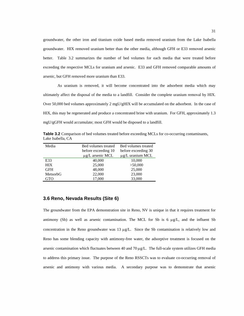
31

groundwater, the other iron and titanium oxide based media removed uranium from the Lake Isabella

groundwater. HIX removed uranium better than the other media, although GFH or E33 removed arsenic

better. Table 3.2 summarizes the number of bed volumes for each media that were treated before

exceeding the respective MCLs for uranium and arsenic. E33 and GFH removed comparable amounts of

arsenic, but GFH removed more uranium than E33.

As uranium is removed, it will become concentrated into the adsorbent media which may

ultimately affect the disposal of the media to a landfill. Consider the complete uranium removal by HIX.

Over 50,000 bed volumes approximately 2 mgU/gHIX will be accumulated on the adsorbent. In the case of

HIX, this may be regenerated and produce a concentrated brine with uranium. For GFH, approximately 1.3

mgU/gGFH would accumulate; most GFH would be disposed to a landfill.

Table 3.2 Comparison of bed volumes treated before exceeding MCLs for co-occurring contaminants, Lake Isabella, CA


Bed volumes treated before exceeding 30 μg/L uranium MCL

E33 40,000 10,000 HIX 25,000 >50,000 GFH 48,000 25,000 MetsorbG 22,000 23,000 GTO 17,000 33,000

3.6 Reno, Nevada Results (Site 6)

The groundwater from the EPA demonstration site in Reno, NV is unique in that it requires treatment for

antimony (Sb) as well as arsenic contamination. The MCL for Sb is 6 μg/L, and the influent Sb

concentration in the Reno groundwater was 13 μg/L. Since the Sb contamination is relatively low and

Reno has some blending capacity with antimony-free water, the adsorptive treatment is focused on the

arsenic contamination which fluctuates between 40 and 70 μg/L. The full-scale system utilizes GFH media

to address this primary issue. The purpose of the Reno RSSCTs was to evaluate co-occurring removal of

arsenic and antimony with various media. A secondary purpose was to demonstrate that arsenic

32

breakthrough curves for GFH are not affected by scaling the RSSCTs to a lower EBCT; a technique that

expedites the RSSCT procedure.


GFH removed arsenic slightly better than the other media (i.e., HIX, ARM200, and Dow GTO) evaluated

on this groundwater (Figure 3.18). This was the first RSSCT with Arm200, which removed arsenic to the

10 µg/L breakthrough for about 8000 bed volumes. Comparatively, HIX and GFH broke through at 9000

and 12,000 bed volumes, respectively. Dow GTO breakthrough occurred at about 5000 bed volumes and

operational problems (pressure accumulation) in the RSSCT column prompted ceasing operation at ~

21,000 bed volumes.

Two RSSCTs were conducted with GFH, based upon different full-scale EBCTs (3 and 6.2

minutes). The loading rates were equal in both RSSCTs and only the media bed length varied between the

3 min (7.8 cm column length) and 6.2 min (16 cm column length) EBCTs. Figure 3.19 demonstrates that

on a bed volume treated basis, there is no difference in the arsenic breakthrough curve; similar results were

observed for other oxyanions (not shown). RSSCTs conducted with shorter EBCTs require less water to

conduct the tests and less operational run time. For example the RSSCT that simulated a 3 min EBCT had

a real EBCTsc of 20 sec and required 10 days of operation compared against an EBCTsc of 40 sec and 17

days of operation for the RSSCT simulating the 6.2 min full-scale EBCT. Therefore, these RSSCTs

conclude that evaluation of a 3 min simulated EBCT results in comparable data as for a longer EBCT, and

offers significant logistical benefits in collecting water and conducting the tests.

3.6.2 Antimony Removal

Most media did not remove significant amounts of antimony from the groundwater (Figure 3.20). The full-

scale system in the field observed antimony in the GFH column effluent after 5,000 bed volumes of

operation. This observation corresponds well with the observed antimony breakthrough from the RSSCT

using GFH. GTO appeared to remove antimony better than the other media, removing antimony to the 6

µg/L breakthrough point for about 20,000 bed volumes. Table 4.3 compares the bed volumes treated until

breakthrough for arsenic and antimony.

33


The water contained low levels of vanadium (4 ppb) and all the media except GTO removed vanadium

almost completely during the RSSCT (Figure 3.21). The water contained moderately high levels of

phosphate (~162 μg/L). Partial phosphate removal was observed by all the media (Figure 3.21). The shape

of the phosphate breakthrough curve is similar to the shape for the arsenic breakthrough curve for each

media (Figure 4.18), although the phosphate breaks through 5000 to 10,000 bed volumes earlier than

arsenic. This suggests that phosphate may be competing for arsenic adsorption sites on the media. Silica

levels were moderately high (23 mg/L) and all the media removed some silica during the first few thousand

bed volumes of operation (Figure 3.21). Silica removal by the media will change the surface chemistry

properties (i.e., lower the zeta potential on the media) and in general will detrimentally impact arsenic

removal. Iron concentrations in the RSSCT effluent were comparable among the different media.

Table 3.3 Comparison of bed volumes treated before exceeding MCLs for co-occurring contaminants, Reno, NV


Bed volumes treated before exceeding 6 μg/L antimony MCL

ARM 200 8000 < 2000 HIX 9000 < 2000 GFH 12,000 < 5000 GTO 5000 20,000

3.7 Arsenic Adsorption Density of Media

In order to compare media, arsenic adsorption capacity (μg As/mg dry media) from the media of the

RSSCTs was calculated. The mass of dry media was determined at 105 oC. The area above the arsenic

breakthrough curve was integrated and divided by the mass of media in the RSSCT. For the purposes of

comparison, the adsorption capacity associated with an effluent arsenic concentration of 10 μg/L was

selected. Table 3.4 summarizes the results. Based upon the measured iron content of each media, the

adsorption capacity is also reported as μgAs/mgFe. GFH and E33 had similar arsenic adsorption capacities

(5 to 6 μgAs/mgFe). AAFS50 had a lower arsenic adsorption capacity based upon the dry media, but a

very high arsenic adsorption capacity based upon iron content. This suggests that the activated aluminum

34

was also responsible for some of the arsenic removal, in addition to the iron (hydr)oxides added to the

AAFS50 product.

Table 3.4 Summary of arsenic adsorption capacities

Arsenic adsorption capacity at an effluent arsenic

concentration of 10 μ/L Site Media

mgAs / g dry media Valley Vista, AZ

E33 GFH AAFS-50 Full-Scale

1.1 1.2 0.3

0.121

Rimrock, AZ

AAFS50 GFH E33 Full-scale HIX

0.13 2.0 1.8 1.21

1.3 Licking Valley School District, OH

AAFS50 GFH E33 HIX

0.05 >1 1

0.3

Lyman, NE

E33 HIX Dow GTO MetsorbG

0.4 0.2 0.3 0.2

Lake Isabella, CA

E33 GFH HIX Dow GTO MetsorbG

1.4 1.4 0.9 0.5 0.6

Reno, NV

ARM 200 GFH HIX Dow GTO

0.3 0.4 0.3 0.2

1Full-scale estimates are based upon approximate masses of media in the vessel and a density of 2.5 g/cm3.

35

3.8 Layne Christensen RSSCTs (Scottsdale, AZ site water)

In addition to the EPA sponsored experiments, there was a set of RSSCTs conducted with the support of

Layne Christensen, a vendor of small system treatment packages. The objective of these RSSCTs was to

evaluate the arsenic removal capacity of newly developed adsorptive media in a typical southwestern US

groundwater matrix (Scottsdale, AZ). These new media were compared against current commercially

available media. Iron-based media from Next, Englehard (ARM200), and Melstream (RS-AF) were

compared against E33. Melstream (RS-AT) is a titanium based media that was compared against Dow.


The iron-based media from Next, performed better than all other iron-based media lasting for about 35,000

bed volumes before reaching the 10 ppb breakthrough (Figure 3.25). E33 broke through at about 24,000

bed volumes while Englehard’s ARM200 broke through at about 18,000 bed volumes. Melstream’s RS-AF,

which is an iron-enriched aluminum based media, performed the poorest and breaking through at about

10,000 bed volumes.

The titanium based media breakthrough curves are shown in Figure 3.26. Dow reached the 10 ppb

breakthrough point at about 20,000 bed volumes while Melstream’s RS-AT lasted for only 8000 bed

volumes.

To compliment the RSSCT breakthrough data, batch isotherm experiments were also conducted

with this water. Figures 3.27 and 3.28 show the results of the iron- and titanium-based media, respectively.

E33, ARM200, and Next media had similar isotherm results. This makes the performance of Next

somewhat surprising. From the isotherm experiments, one wouldn’t necessarily expect Next to outperform

E33 by 10,000 bed volumes. However, the relatively close breakthrough of E33 and ARM200 is supported

by the isotherm data.

The isotherm data for the titanium media is somewhat unclear with the variability of the

Melstream RS-AT data points. However, the breakthrough data clearly defines Dow’s performance as

superior to that of Melstream RS-AT.

36


The Scottsdale groundwater was found to contain about 8 ppb of phosphorous and about 44 ppb of

vanadium. Figure 3.29 shows the breakthrough curves for these adsorbates.

All media showed a capacity to remove phosphorous with Next, ARM200, and E33 performing

very similarly. Vanadium performance among the iron-based media resembles the arsenic performance

with Next removing vanadium longer than ARM200 and E33. Titanium dioxide media seems to have a

high capacity for vanadium as there was minimal effluent vanadium concentration at about 24,000 bed

volumes.

3.8.3 Summary of Results

Next’s arsenic adsorption media was found to remove arsenic for about 10,000 bed volumes longer than

E33 and about 17,000 bed volumes longer than Englehard’s ARM200. Melstream’s RS-AF only lasted for

10,000 bed volumes and the RS-AT titanium-based media lasted for 8000 bed volumes. All media showed

some phosphorous and vanadium removal capacity while the titanium media seem to excel at vanadium

removal.

37

0

5

10

15

20

25

30

35

40

45

50

- 20,000 40,000 60,000 80,000 100,000

Bed Volumes Treated

Effl

uent

Ars

enic

con

cent

ratio

n (p

pb)

AAFS-50GFHE33

Fig. 3.1. Valley Vista RSSCT field data for arsenic breakthrough (Badruzzaman, 2005)

38

Fig. 3.2. Field data for arsenic-competing ions (V, P, Si, Al) breakthrough from Valley Vista, AZ (Badruzzaman, 2005)

0

5

10

15

20

25

30

35

40

45

- 20,000 40,000 60,000 80,000 100,000

Bed volumes treated

Effl

uent

Ars

enic

Con

c (p

pb)

AAFS50E33 (ReSch=2000)GFHE33 (ReSch=500)

Fig. 3.3. Lab RSSCT arsenic data for Valley vista, AZ (Badruzzaman, 2005)

0

5

10

15

20

- 20,000 40,000 60,000 80,000 100,000

Bed Volumes Treated

Efflu

ent V

anad

ium

Con

cent

ratio

n (p

pb) .

AAFS50GFHE33 (ReSc=2000)

Influent Conc = 15 ppb

0

5

10

15

20

25

30

- 20,000 40,000 60,000 80,000 100,000

Bed Volumes Treated

Efflu

ent T

otal

P C

once

ntra

tion

(ppb

) .



0

2

4

6

8

10

12

14

16

18

20

- 20,000 40,000 60,000 80,000 100,000

Bed Volumes Treated

Effl

uent

Silic

a C

once

ntra

tion

(ppm

) .


Influent Conc = 18.5 ppm

0

5

10

15

- 20,000 40,000 60,000 80,000 100,000

Bed Volumes Treated

Efflu

ent I

ron

Con

cent

ratio

n (p

pb) .


Influent Conc = 3.8 ppb

39

0

5

10

15

20

25

30

35

40

45

0 20,000 40,000 60,000 80,000 100,000Bed Volumes Treated

Effl

uent

Ars

enic

Con

c (p

pb)

E33 (Field)E33 (Lab)GFH (Field)GFH (Lab)

Fig. 3.4. A comparison of RSSCT lab data versus RSSCT field data for Valley Vista, AZ (Badruzzaman, 2005)

40

0

5

10

15

20

25

30

35

40

45

0 10 20 30 40 50 60 70Bed Volumes Treated (in thousands)

Efflu

ent A

rsen

ic C

onc

(ppb

)

Tank 1RSSCT (Field)RSSCT (Lab)

Fig. 3.5. Comparison of Lab/Field RSSCT versus Full-scale system (AAFS50) (Badruzzaman, 2005)

0

10

20

30

40

50

60

70

80

- 20,000 40,000 60,000 80,000 100,000

Bed Volumes Treated

Effl

uent

Ars

enic

Con

cent

ratio

n (p

pb) .

AAFS50GFHE33E33 Full ScaleHIX

Fig. 3.6. RSSCT arsenic data for Rimrock, AZ (Badruzzaman, 2005)

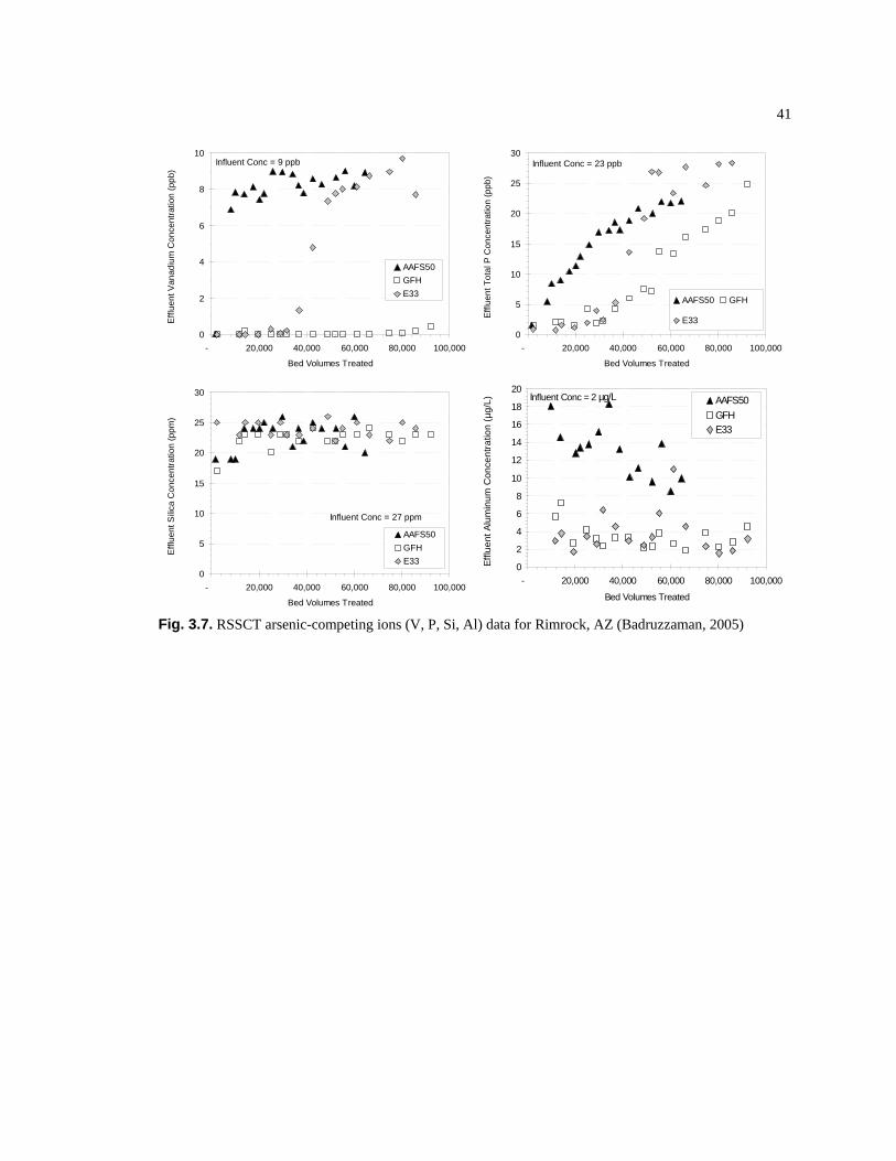
41

Fig. 3.7. RSSCT arsenic-competing ions (V, P, Si, Al) data for Rimrock, AZ (Badruzzaman, 2005)

0

2

4

6

8

10

- 20,000 40,000 60,000 80,000 100,000

Bed Volumes Treated

Efflu

ent V

anad

ium

Con

cent

ratio

n (p

pb) .

AAFS50GFHE33


0

5

10

15

20

25

30

- 20,000 40,000 60,000 80,000 100,000

Bed Volumes Treated

Efflu

ent T

otal

P C

once

ntra

tion

(ppb

) .

AAFS50 GFH

E33


0

5

10

15

20

25

30

- 20,000 40,000 60,000 80,000 100,000

Bed Volumes Treated

Effl

uent

Silic

a C

once

ntra

tion

(ppm

) .

AAFS50GFHE33

Influent Conc = 27 ppm

0

2

4

6

8

10

- 20,000 40,000 60,000 80,000 100,000

Bed Volumes Treated

Efflu

ent I

ron

Con

cent

ratio

n (p

pb) .

AAFS50 GFH

E33

Influent Conc = 3.4 ppb

0

2

4

6

8

10

12

14

16

18

20

- 20,000 40,000 60,000 80,000 100,000

Bed Volumes Treated

Efflu

ent A

lum

inum

Con

cent

ratio

n (µ

g/L)

.

AAFS50GFHE33

Influent Conc = 2 µg/L

42

Fig. 3.8. RSSCT Results for Licking Valley School District, Newark, OH (Badruzzaman, 2005)

0

10

20

30

40

50

60

70

80

0 5,000 10,000 15,000 20,000 25,000

Bed Volumes Treated

Effl

uent

Ars

enic

Con

c (p

pb) .

GFH (RSSCT) E33(RSSCT)FS-50(RSSCT) GFH (Pilot)E33(Pilot) FS-50(Pilot)

Fig. 3.9. Comparison of RSSCTs with Pilot-scale Results for Licking Valley School District, Newark, OH (Badruzzaman, 2005)

0

10

20

30

40

50

60

70

- 5,000 10,000 15,000 20,000 25,000

Bed Volumes Treated

Effl

uent

Ars

enic

Con

cent

ratio

n (p

pb) .

AAFS50GFHE33HIX

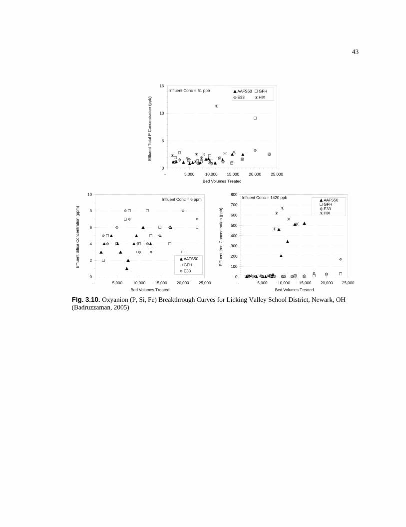
43

Fig. 3.10. Oxyanion (P, Si, Fe) Breakthrough Curves for Licking Valley School District, Newark, OH (Badruzzaman, 2005)

0

100

200

300

400

500

600

700

800

- 5,000 10,000 15,000 20,000 25,000

Bed Volumes Treated

Efflu

ent I

ron

Con

cent

ratio

n (p

pb) .

AAFS50GFHE33HIX


0

2

4

6

8

10

- 5,000 10,000 15,000 20,000 25,000

Bed Volumes Treated

Effl

uent

Silic

a C

once

ntra

tion

(ppm

) .

AAFS50GFHE33


0

5

10

15

- 5,000 10,000 15,000 20,000 25,000

Bed Volumes Treated

Efflu

ent T

otal

P C

once

ntra

tion

(ppb

) . AAFS50 GFH

E33 HIX


44

0

5

10

15

20

25

30

- 10,000 20,000 30,000 40,000 50,000 60,000

Bed Volumes Treated

Effl

uent

Ars

enic

Con

cent

ratio

n (p

pb) .

E33HIXGTOMetsorbG

Fig. 3.11. RSSCT arsenic data for Lyman, NE

45

0

0.2

0.4

0.6

0.8

1

- 20,000 40,000 60,000 80,000

Bed Volumes Treated

Effl

uent

Ars

enic

Con

cent

ratio

n (p

pb) .

GTO (ReSc=1000)MetsorbG (ReSc=1000)GTO (ReSc=2000)MetsorbG (ReSc=2000)

Fig. 3.12. Breakthrough data comparison of titanium dioxide media (GTO and MetsorbG) columns packed using Reynold-Schmidt numbers of 1000 and 2000 for Lyman, NE

46

q = .38Ce.81

R2 = 0.89

q = .28Ce.60

R2 = 0.94

q = .06Ce1.15

R2 = 0.93

q = .04Ce1.03

R2 = 0.59

-0.8

-0.6

-0.4

-0.2

0

0.2

0.4

0.6

-0.4 -0.2 0 0.2 0.4 0.6 0.8 1 1.2 1.4

Log Ce

Log

q

E33

AsXnp

MetsorbG

Dow

Fig. 3.13. Isotherm experiments for media used in Lyman, NE water

47

Fig. 3.14. RSSCT oxyanion (U, V, Fe, Mn) breakthrough data for Lyman, NE

0

10

20

30

40

50

60

70

80

90

- 10,000 20,000 30,000 40,000 50,000 60,000

Bed Volumes Treated

Efflu

ent U

rani

um C

once

ntra

tion

(ppb

) .

E33HIXGTOMetsorbG


0

5

10

15

20

25

30

35

40

45

- 10,000 20,000 30,000 40,000 50,000 60,000

Bed Volumes Treated

Efflu

ent V

anad

ium

Con

cent

ratio

n (p

pb) .

E33HIXGTOMetsorbG


0

5

10

15

- 10,000 20,000 30,000 40,000 50,000 60,000

Bed Volumes Treated

Efflu

ent I

ron

Con

cent

ratio

n (p

pb) .

E33HIXGTOMetsorbG

0

10

20

30

40

50

60

70

80

- 10,000 20,000 30,000 40,000 50,000 60,000

Bed Volumes Treated

Effl

uent

Man

gane

se C

once

ntra

tion

(ppb

) . E33HIXGTOMetsorbG

48

0

10

20

30

40

50

- 20,000 40,000 60,000 80,000

Bed Volumes Treated

Effl

uent

Ars

enic

Con

cent

ratio

n (p

pb) . E33

HIXGFHMetsorbG (ReSc=1000**)GTO (ReSc=1000**)

Fig. 3.15. Lake Isabella RSSCT arsenic data which simulated an EBCT of 5.3 min except ** which required a simulated EBCT of 2.5 min

0

5

10

15

20

25

30

35

40

- 20,000 40,000 60,000 80,000

Bed Volumes Treated

Effl

uent

Ars

enic

Con

cent

ratio

n (p

pb) .

GTO (ReSc=1000)GTO (ReSc=2000)MetsorbG (ReSc=1000)

Fig. 3.16. Comparison of titanium dioxide (GTO and MetsorbG) media RSSCTs conducted with Reynold-Schmidt numbers of 1000 or 2000 in Lake Isabella RSSCTS

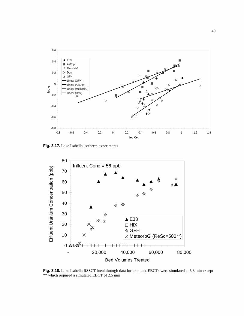
49

-0.8

-0.6

-0.4

-0.2

0

0.2

0.4

0.6

-0.8 -0.6 -0.4 -0.2 0 0.2 0.4 0.6 0.8 1 1.2 1.4

log Ce

log

q

E33AsXnpMetsorbGDowGFHLinear (GFH)Linear (AsXnp)Linear (MetsorbG)Linear (Dow)

Fig. 3.17. Lake Isabella isotherm experiments

0

10

20

30

40

50

60

70

80

- 20,000 40,000 60,000 80,000

Bed Volumes Treated

Effl

uent

Ura

nium

Con

cent

ratio

n (p

pb) .

E33HIXGFHMetsorbG (ReSc=500**)


Fig. 3.18. Lake Isabella RSSCT breakthrough data for uranium. EBCTs were simulated at 5.3 min except ** which required a simulated EBCT of 2.5 min

50

0

10

20

30

40

50

60

- 20,000 40,000 60,000 80,000

Bed Volumes Treated

Effl

uent

Ura

nium

Con

cent

ratio

n (p

pb) .

GTO (ReSc=1000)GTO (ReSc=2000)MetsorbG (ReSc=1000)

Influent Uranium: 56 ppbGTO media started to exit RSSCT at 42,000 BV

Fig. 3.19. Comparison of titanium dioxide media (GTO and MetsorbG) for Lake Isabella RSSCT uranium breakthrough data. EBCT was simulated at 2.5 min

0

10

20

30

40

50

60

70

- 10,000 20,000 30,000 40,000 50,000

Bed Volumes Treated

Effl

uent

Ars

enic

Con

cent

ratio

n (p

pb) .

HIXARM200GTO (ReSc=1000)GFH

Fig. 3.20. Arsenic breakthrough data from Reno, NV RSSCTs. EBCTs were simulated at 3 min.

51

q = .16Ce.36

R2 = 0.75

q = .26Ce.71

R2 = 0.86

q= .26Ce.39

R2 = 0.81

q = .18Ce.36

R2 = 0.31

-0.6

-0.5

-0.4

-0.3

-0.2

-0.1

0

0.1

0.2

0.3

0.4

0.5 0.7 0.9 1.1 1.3 1.5 1.7

log Ce

log

q ARM200

AsXnp

Dow

GFH

Fig. 3.21. Reno isotherm experiments

0

10

20

30

40

50

60

- 10,000 20,000 30,000 40,000 50,000

Bed Volumes Treated

Effl

uent

Ars

enic

Con

cent

ratio

n (p

pb) .

GFH (Simulated EBCT = 3 min)

GFH (Simulated EBCT = 6.2 min)

Fig. 3.22. Comparison of GFH columns packed at 3 & 6.2 min. EBCTs for Reno RSSCTs

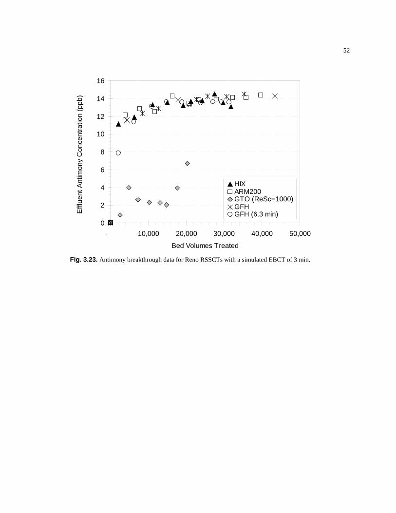
52

0

2

4

6

8

10

12

14

16

- 10,000 20,000 30,000 40,000 50,000

Bed Volumes Treated

Effl

uent

Ant

imon

y C

once

ntra

tion

(ppb

) .

HIXARM200GTO (ReSc=1000)GFH GFH (6.3 min)

Fig. 3.23. Antimony breakthrough data for Reno RSSCTs with a simulated EBCT of 3 min.

53

Fig. 3.24. Oxyanion breakthrough data for Reno RSSCTs with a simulated EBCT of 3 min.

Inf luent As conc. = 20 ppb

0

5

10

15

20

25

0 20000 40000 60000 80000

Bed Volumes Treated

Efflu

ent A

s C

onc.

[ppb

]

NEXTEnglehardE33Mel RS-AF

Fig. 3.25. Arsenic breakthrough curves for Layne Christensen RSSCTs with iron-based media

0

1

2

3

4

- 10,000 20,000 30,000 40,000 50,000

Bed Volumes Treated

Effl

uent

Van

adiu

m C

once

ntra

tion

(ppb

) .HIXARM200GTO (ReSc=1000)GFH


0

20

40

60

80

100

120

140

160

180

200

- 10,000 20,000 30,000 40,000 50,000

Bed Volumes Treated

Efflu

ent T

otal

P C

once

ntra

tion

(ppb

) .



0

5

10

15

20

25

30

- 10,000 20,000 30,000 40,000 50,000

Bed Volumes Treated

Effl

uent

Silic

a C

once

ntra

tion

(ppm

) .



0

5

10

15

- 10,000 20,000 30,000 40,000 50,000

Bed Volumes Treated

Efflu

ent I

ron

Con

cent

ratio

n (p

pb) .


54

Influent As conc. = 20 ppb

0

5

10

15

20

25

0 10000 20000 30000 40000 50000 60000 70000

Bed Volumes Treated

Efflu

ent A

s C

onc.

[ppb

]

Dow

Mel RS-AT

Fig. 3.26. Arsenic breakthrough curves for Layne Christensen RSSCTs with titanium-based media

Scottsdale water pH=8.6

-0.8

-0.6

-0.4

-0.2

0

0.2

0.4

0.6

0.8

-0.5 0 0.5 1 1.5

Log Ce

Log

q [u

g As

/mg

Dow

]

E33Melstream AFEnglehardNext

Fig. 3.27. Batch isotherm data for the iron-based media (and Melstream RS-AF)

55

Scottsdale water pH=8.6

-0.6

-0.4

-0.2

0

0.2

0.4

0.6

0.8

-0.1 0.1 0.3 0.5 0.7 0.9 1.1 1.3 1.5

Log Ce

Log

q [u

g As

/mg

Dow

]

DowMelstream ATLinear (Dow)Linear (Melstream AT)

Fig. 3.28. Batch isotherm data for the titanium based media

0

2

4

6

8

10

12

0 20000 40000 60000

Bed Volumes

Efflu

ent P

Con

c. [p

pb]

NEXT ARM200E33 RS-AFDow RS-AT

0

5

10

15

20

25

30

35

40

45

0 20000 40000 60000

Bed Volumes

Efflu

ent V

Con

c. [p

pb]

NEXT ARM200E33 RS-AFDow RS-AT

Fig. 3.29. Phosphorous and vanadium breakthrough curves for the Layne Christensen RSSCTs

56

CHAPTER 4: REMOVAL OF METALS CO-OCCURRING WITH ARSENIC This chapter takes a closer look at the removal of metals that co-occur with arsenic in the groundwaters of

this study. The objective here is to fit the breakthrough curves of the various adsorbates with the Thomas

equation in order to compare their adsorption characteristics across varied media and groundwater matrices.

In addition to the RSSCTs that were conducted for the EPA funded project, the set of RSSCTs conducted

for Layne Christensen is included.

4.1 Determination of Thomas Fit Parameters

Once the RSSCT effluent samples were analyzed by ICP-MS or GFAA, the data could be plotted as to

produce breakthrough curves. The aim was to then fit the breakthrough data with an empirical model to

compare the absorptive behavior of each solute. The empirical model utilized in this research was the

Thomas Equation (Reynolds and Richards, 1996):

( )

⎟⎟⎠

⎞⎜⎜⎝

⎛+

=− VCmq

Qke

e

CC00

1

1/ 0

where:

Ce = Effluent concentration [ppb]

C0 = Influent concentration [ppb]

Q = flow rate [mL/min]

m = mass of media [g]

k = Thomas rate constant [mL/min.µg]

q0 = maximum solid phase concentration [µg/g]

V = bed volumes treated [L]

Microsoft Excel was used to simultaneously fit the Thomas rate constant, k, as well as the

maximum solid phase concentration, q0. This was done on a trial and error basis by plotting the Thomas fit

57

line over the experimental data and adjusting the k and q0 values until a visual confirmation of a good fit

was made. Figure 4.1 is an example of the experimental data fitted with the Thomas equation estimation.

By adjusting the Thomas rate constant, k, one can adjust the “steepness” of the breakthrough curve.

Similarly, by adjusting the maximum solid phase concentration, q0, the point along the x-axis where the

data begins to breakthrough can be controlled. Figures 4.2 and 4.3 show the effect of adjusting k and q0 on

the Thomas curve fit, respectively.

Lowering the k value will model a breakthrough over a longer period of bed volumes. Conversely,

raising the k value will model a faster breakthrough (Figure 4.2).

Lowering q0 will shift the breakthrough curve horizontally to an earlier bed volume. Conversely,

raising q0 will model the breakthrough at a later bed volume (Figure 4.3).

The beginning portion of the breakthrough curve was the visual target for the best fit for two

reasons. First, data will be compared around the 10 ppb breakthrough point for arsenic. Second, there

were some adsorbates that showed abnormal breakthrough behaviors toward the end of the tests, which

cannot be modeled accurately by the Thomas fit (Figure 4.4). However, in most of these cases, the

beginning portion of the breakthrough curve can still be modeled by the Thomas equation. The efficiency

of the data fits were quantified by plotting the observed data versus the Thomas fit prediction data. A

linear regression fit of this graph yields an R2 value for the Thomas fit of observed data (Table 4.1).

While the examples above show the occasions of poor fit, in general, the Thomas fit matches the

observed data very well. Figure 4.5 displays common examples of the Thomas equation as an appropriate

model to observed breakthrough data for various adsorbates.

Breakthrough data was obtained for the various metals of concern for each set of RSSCTs. The

Thomas fit was applied to all curves in which sufficient data points were collected in order to compare the

adsorption tendencies of multiple metals for different media in various groundwater matrices. The Thomas

fit parameter, q0, coupled with the quantity of bed volumes treated to a specified breakthrough, can show

the relative efficiency of each media to remove a particular metal. The R2 value in Table 4.1 shows the

accuracy of the Thomas fit to match the observed data.

58

Table 4.1. Thomas fit parameters k and q0 for various solutes (As, U, Sb, P, V, Mn) and adsorptive media

Site/Water Media k q0 R2k q0 R2

k q0 R2

Lake Isabella E33 0.000057 111250 0.9898 0.000241 36010 0.9662 - - -pH = 7.2 AsXnp 0.000184 44500 0.9632 ND ND ND - - -

As, 41[ppb] GFH 0.000054 130000 0.9845 0.000040 72854 0.9669 - - -U, 56 [ppb] MetsorbG 0.000048 150000 0.9613 0.000021 168750 0.7572 - - -P, 15 [ppb] Dow (1000) 0.000026 170000 0.9275 0.000013 299050 0.9211 - - -

Dow (2000) 0.000085 58000 0.9502 0.000045 90000 0.961 - - -

Layne Christensen Next 0.000080 110000 0.9247 - - - - - -(Scottsdale, AZ water) Arm200 0.000186 55000 0.9538 - - - - - -

pH = 8.4 E33 0.000166 68000 0.928 - - - - - -As, 20 [ppb] Dow 0.000176 57000 0.9422 - - - - - -P, 8 [ppb] Melstream RS-AT 0.000216 29000 0.9539 - - - - - -V, 42 [ppb] Melstream RS-AF 0.000266 37000 0.9433 - - - - - -

Lyman E33 0.000184 71000 0.9705 0.003194 3000 0.8776 - - -pH = 7.7 AsXnp 0.000324 26000 0.9947 0.000594 51000 0.9053 - - -

As, 22 [ppb] Dow 0.000086 75000 0.9896 0.000814 5000 0.968 - - -P, 54 [ppb] MetsorbG 0.000114 42000 0.9903 0.001941 1000 0.983 - - -V, 37 [ppb]

Reno Arm200 0.000134 75000 0.9929 - - - 0.004241 4000 0.9766pH = 7.4 Dow 0.000044 100000 0.8286 - - - 0.000194 35000 0.5994

As, 51[ppb] AsXnp 0.000294 29000 0.9909 - - - 0.005004 800 0.9679Sb, 12.5 [ppb] GFH(3) 0.000074 110000 0.938 - - - 0.002314 2500 0.9627P, 160 [ppb] GFH(6) 0.000098 52000 0.9806 - - - 0.002014 1200 0.9725


k q0 R2

Rimrock, AZ AAFS-50 0.000314131 19000 0.9572 - - - - - -pH = 7.5-7.7 GFH 0.000028 270000 0.9542 - - - - - -As, 62 [ppb] E33 0.000032131 230000 0.907 - - - - - -P, 23 [ppb] V, 9 [ppb]

Valley Vista, AZ AAFS-50 0.000214131 26000 0.8342 - - - - - -(field tests) GFH 0.000054131 145000 0.9304 - - - - - -

pH = 7.5-8.0 E33 0.000045131 148000 0.778 - - - - - -As, 40 [ppb]P, 19 [ppb] V, 15 [ppb]

Valley Vista, AZ AAFS-50 0.000214131 14000 0.9187 - - - - - -(lab tests) GFH 0.000044131 140000 0.9677 - - - - - -

pH = 7.5-8.0 E33 0.000038131 155000 0.9624 - - - - - -As, 40 [ppb]

Columbus, OH AAFS-50 0.000094131 21000 0.9534 - - - - - -pH = 8.1 GFH 0.000114131 142000 0.9065 - - - - - -

As (III), 66 [ppb] E33 0.000094131 65000 0.8911 - - - - - -P, 51 [ppb] ArsenXnp 0.000284131 23000 0.9664 - - - - - -

Mn, 183 [ppb]

As U Sb

As U Sb

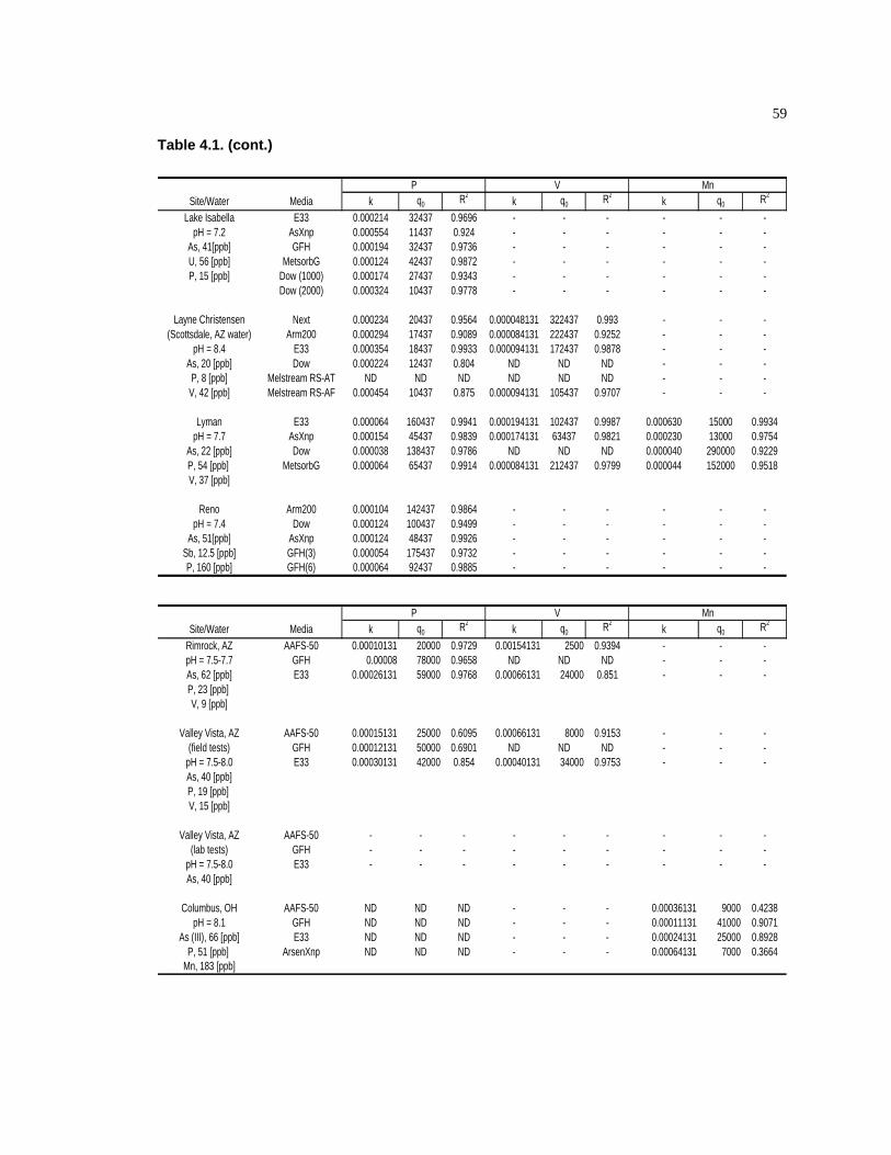
59

Table 4.1. (cont.)


k q0 R2

Lake Isabella E33 0.000214 32437 0.9696 - - - - - -pH = 7.2 AsXnp 0.000554 11437 0.924 - - - - - -

As, 41[ppb] GFH 0.000194 32437 0.9736 - - - - - -U, 56 [ppb] MetsorbG 0.000124 42437 0.9872 - - - - - -P, 15 [ppb] Dow (1000) 0.000174 27437 0.9343 - - - - - -

Dow (2000) 0.000324 10437 0.9778 - - - - - -

Layne Christensen Next 0.000234 20437 0.9564 0.000048131 322437 0.993 - - -(Scottsdale, AZ water) Arm200 0.000294 17437 0.9089 0.000084131 222437 0.9252 - - -

pH = 8.4 E33 0.000354 18437 0.9933 0.000094131 172437 0.9878 - - -As, 20 [ppb] Dow 0.000224 12437 0.804 ND ND ND - - -P, 8 [ppb] Melstream RS-AT ND ND ND ND ND ND - - -V, 42 [ppb] Melstream RS-AF 0.000454 10437 0.875 0.000094131 105437 0.9707 - - -

Lyman E33 0.000064 160437 0.9941 0.000194131 102437 0.9987 0.000630 15000 0.9934pH = 7.7 AsXnp 0.000154 45437 0.9839 0.000174131 63437 0.9821 0.000230 13000 0.9754

As, 22 [ppb] Dow 0.000038 138437 0.9786 ND ND ND 0.000040 290000 0.9229P, 54 [ppb] MetsorbG 0.000064 65437 0.9914 0.000084131 212437 0.9799 0.000044 152000 0.9518V, 37 [ppb]

Reno Arm200 0.000104 142437 0.9864 - - - - - -pH = 7.4 Dow 0.000124 100437 0.9499 - - - - - -

As, 51[ppb] AsXnp 0.000124 48437 0.9926 - - - - - -Sb, 12.5 [ppb] GFH(3) 0.000054 175437 0.9732 - - - - - -P, 160 [ppb] GFH(6) 0.000064 92437 0.9885 - - - - - -

Site/Water Media k q0 R2 k q0 R2 k q0 R2

Rimrock, AZ AAFS-50 0.00010131 20000 0.9729 0.00154131 2500 0.9394 - - -pH = 7.5-7.7 GFH 0.00008 78000 0.9658 ND ND ND - - -As, 62 [ppb] E33 0.00026131 59000 0.9768 0.00066131 24000 0.851 - - -P, 23 [ppb] V, 9 [ppb]

Valley Vista, AZ AAFS-50 0.00015131 25000 0.6095 0.00066131 8000 0.9153 - - -(field tests) GFH 0.00012131 50000 0.6901 ND ND ND - - -

pH = 7.5-8.0 E33 0.00030131 42000 0.854 0.00040131 34000 0.9753 - - -As, 40 [ppb]P, 19 [ppb] V, 15 [ppb]

Valley Vista, AZ AAFS-50 - - - - - - - - -(lab tests) GFH - - - - - - - - -

pH = 7.5-8.0 E33 - - - - - - - - -As, 40 [ppb]

Columbus, OH AAFS-50 ND ND ND - - - 0.00036131 9000 0.4238pH = 8.1 GFH ND ND ND - - - 0.00011131 41000 0.9071

As (III), 66 [ppb] E33 ND ND ND - - - 0.00024131 25000 0.8928P, 51 [ppb] ArsenXnp ND ND ND - - - 0.00064131 7000 0.3664

Mn, 183 [ppb]

V MnP

MnVP

60

4.2 Co-Removal of Antimony (Sb):

One of the four test locations had significant antimony concentrations (Reno, ~13 ppb). At this location

four media were tested; Englehard ARM200, ArsenXnp, GFH, and Dow Absorbsia. The iron-based media

(ARM200, GFH) and Ion Exchange Resin (ArsenXnp) showed very little capacity to remove antimony.

Table 4.2 shows the Thomas Fit q0 parameter for the titanium dioxide media (Dow Absorbsia) being

significantly greater than that of the other media. Subsequently, Dow showed the greatest removal capacity

by removing Sb for over 20,000 bed volumes before reaching the 6 ppb breakthrough point. It is important

to note that the Dow column lost about 1/3 of its media throughout the course of the RSSCT.

Table 4.2. Thomas Fit Parameters for Sb (Reno RSSCT)

Media k [ml/min.mg]

q0 [mg/g]

Bed Volumes Treated to Sb MCL (6 ppb)

ArsenXnp 0.0050 800 1200 GFH(3 min EBCT) 0.0023 2500 2000

GFH(6.2 min EBCT) 0.0020 1200 2000 Englehard ARM200 0.0042 4000 2000 Dow (ReSc# =1000) 0.0002 35000 19000

It is important to remember that the primary reason for these RSSCTs was to remove arsenic.

While Dow Absorbsia was most efficient at removing antimony, it was not the best media for removing

arsenic. Figure 4.6 is a comparison of the arsenic removal performance of the four media used for the Reno

groundwater.

Dow Absorbsia was only able to treat the groundwater to the 10 ppb As level for about 5000 bed

volumes. All other media outperformed Dow Absorbsia in arsenic removal. The iron hydroxide media

(GFH) removed arsenic for the longest time, lasting until about 12,000 bed volumes.

4.3 Co-Removal of Uranium (U):

Of the four test locations, Lyman, NE and Lake Isabella, CA had uranium concentrations of 40 and 56 ppb,

respectively. In both of these sets of RSSCTs the HIX ArsenXnp resin showed a high capacity to co-

61

remove uranium alongside arsenic (see Table 4.3). At Lyman, ArsenXnp was the only media that showed

significant uranium removal.

Table 4.3. Thomas Fit parameters and bed volumes treated to the MCL for U removal in Lake Isabella

and Lyman RSSCTs

Lake Isabella Lyman

Media k

[ml/min.mg] q0

[mg/g]

Bed Volumes Treated to

uranium MCL (30 ppb)

k [ml/min.mg] q0 [mg/g]

Bed Volumes

Treated to uranium MCL (30

ppb) ArsenXnp ND >110000 > 51000 0.00059 51000 20000

GFH 0.00004 75000 26000 - - - E33 0.00019 36000 12000 0.00319 3000 1600

MetsorbG 0.00002 165000 ~25000 0.00194 1000 1200 Dow (Re-

1000) 0.00002 285000 44000 0.00081 5000 1200 Dow (Re-

2000) 0.00005 90000 27000 - - -

Note that in the above table there is no data available for the k parameter for ArsenXnp in the Lake

Isabella RSSCT. This is because ArsenXnp was still removing uranium at the end of the test when the

column was shut down. Therefore, the Thomas fit could not fully be applied to the data, but one could

estimate that the minimum value for q0 is greater than 110,000 since breakthrough had not begun by the

end of the test (~51,000 Bed volumes).

Figures 4.7 and 4.8 show arsenic removal comparisons for all the media used in the Lake Isabella

and Lyman RSSCTs, respectively. As mentioned earlier, it is important to evaluate how each media co-

removes uranium with arsenic.

Basing evaluation on the bed volumes treated until 10 ppb arsenic breakthrough, ArsenXnp is

consistently outperformed by iron-based adsorption media (E33 and GFH) for arsenic removal. MetsorbG

(titanium dioxide) performed similarly with Lyman water, but broke through about 8000-10000 bed

volumes earlier than ArsenXnp with Lake Isabella water. Dow Absorbsia (titanium dioxide) lasted about

5000 bed volumes longer than ArsenXnp with Lyman water.

62

4.4 Co-Removal of Phosphorous (P) and Vanadium (V):

In most of the waters that were tested with significant phosphorous and vanadium levels, the breakthrough

curves of these elements generally coincided with the arsenic breakthrough curve (see Figure 4.9).

This data suggests that these elements might be competing with arsenic for binding sites on the

media. Because of the coincident breakthrough curves one could hypothesize that the adsorption kinetics

of arsenic, phosphorous and vanadium are similar.

Table 4.4 displays the Thomas fit parameters as well as the number of bed volumes treated to 30

ppb for vanadium in the Scottsdale and Lyman waters. While vanadium does not have a specified MCL

from the EPA, some state governments suggest 30 ppb as a guideline for treatment.

Table 4.4. Thomas Fit parameters for V removal in Layne Christensen and Lyman RSSCTs

Layne Christensen – Scottsdale Water Lyman

Media k

[ml/min.mg] q0 [mg/g] Bed Volumes

Treated to 30 ppb k

[ml/min.mg] q0 [mg/g]

Bed Volumes Treated

to 30 ppb

ArsenXnp - - - 0.00017 63000 30000 E33 0.00009 172000 32000 0.00019 102000 27000

MetsorbG - - - 0.00008 212000 > 48000 Dow (Re-

1000) ND ND > 23000 ND ND > 50000

Englehard ARM200 0.00008 222000 45000 - - -

Next 0.00005 322000 60000 - - - Melstream

RS-AF 0.00009 105000 22000 - - -

Melstream RS-AT ND ND > 15000 - - -

Again, the titanium dioxide media columns were not run for enough bed volumes to capture the

vanadium breakthrough. Thus, k and q0 values could not be determined. Titanium dioxide seems to have a

high capacity for vanadium.

Table 4.5 shows the bed volumes treated to 50% of the RSSCT influent phosphorous

concentration. Because there is no current MCL for phosphorous and the Scottsdale water phosphorous

concentration was as low as 8 ppb, the 50% breakthrough was arbitrarily chosen for comparison between

RSSCTs.

63

Table 4.5. Bed Volumes Treated to 50% of Influent Concentration of Phosphorous

Media

Layne Christensen – Scottsdale Water

(P, 8 ppb)

Lyman (P, 54 ppb)

Lake Isabella (P, 15 ppb)

Reno (P, 160 ppb)

ArsenXnp - 12000 23000 5500 E33 17000 24000 41000 -

MetsorbG - 12000 22000 - Dow (Re-

1000) 10000 18000 - 4000

GFH - - 41000 11000 (3minEBCT), 11000(6.2minEBCT)

Englehard ARM200 19000 - - 8000

Next 20000 - - - Melstream

RS-AF 10000 - - -

Melstream RS-AT 6000 - - -

The above data show that all media have a capacity to co-remove phosphorous with arsenic. Lake Isabella

data strongly suggests that phosphorous may have more fouling effects on iron-based media than ion

exchange or titanium dioxide. That same trend is echoed in Lyman and Reno RSSCTs where E33, GFH

and Englehard ARM200 removed phosphorous for more bed volumes than the HIX and titanium dioxide.

4.5 Mass of solute removed per media

Table 4.6 shows the data calculated for specific solute removal capacity for each media on a µmol of solute

per mg of media basis. The total mass of solute adsorbed was found by evaluating the area above the

Thomas fit curve and below the influent solute concentration up to the bed volume point of full arsenic

breakthrough (see Figure 4.10). This value can then be divided by the dry mass of media used in the

RSSCT to yield the specific solute adsorption capacity. Thus, the results show the mass of each solute

adsorbed to the media at the time that the column is fully exhausted for arsenic treatment.

64

Table 4.6. Solute Mass Removal Densities for each media calculated at full As breakthrough

arsenic uranium antimony phosphorous vanadium

Site/Water Media

Bed Volumes treated to full As

breakthrough

qT, Total from As,U,Sb,P,V

[µmol/mg media]qAs [µmol

As/mg media]qU [µmol

U/mg media]qSb [µmol

Sb/mg media]qP [µmol

P/mg media]qV [µmol

V/mg media]Lake Isabella E33 70000 0.0113 0.0074 0.0022 0.0017

pH = 7.2 AsXnp 40000 0.0099 0.0032 0.0059 0.0007As, 41[ppb] GFH 70000 0.0133 0.0073 0.0042 0.0017U, 56 [ppb] MetsorbG NA* NA* NA* NA* NA*P, 15 [ppb] Dow (1000) 50000 0.0155 0.0056 0.0091 0.0009

Dow (2000) NA* NA* NA* NA* NA*

Layne Christensen Next 73000 0.0127 0.0029 0.0012 0.0085(Scottsdale, AZ water) Arm200 67000 0.0094 0.0017 0.0006 0.0071

pH = 8.4 E33 74000 0.0060 0.0015 0.0004 0.0040As, 20 [ppb] Dow 23000 0.0081 0.0018 0.0004 0.0059P, 8 [ppb] Melstream RS-AT 26000 0.0056 0.0005 0.0002 0.0050V, 42 [ppb] Melstream RS-AF 74000 0.0044 0.0010 0.0003 0.0030

Lyman E33 48000 0.0094 0.0020 0.0000 0.0045 0.0029pH = 7.7 AsXnp 25000 0.0064 0.0009 0.0018 0.0015 0.0021

As, 22 [ppb] Dow 46000 0.0160 0.0024 0.0001 0.0055 0.0080P, 54 [ppb] MetsorbG 48000 0.0050 0.0010 0.0000 0.0015 0.0025V, 37 [ppb]

Mn, 70 [ppb]U, 40 [ppb]

Reno Arm200 28000 0.0078 0.0028 0.0001 0.0049pH = 7.4 Dow NA* NA* NA* NA* NA*

As, 51[ppb] AsXnp 19000 0.0028 0.0012 0.0000 0.0016Sb, 12.5 [ppb] GFH(3) 43000 0.0077 0.0032 0.0000 0.0045P, 160 [ppb] GFH(6) 35000* 0.0081 0.0031 0.0000 0.0050

*did not reach full exhaustion The above table is effective at showing a comparison of the proportions of the various solutes that are

adsorbed by each media. For example, for Lake Isabella water, E33’s capacity to remove arsenic was

about 65% of its capacity to remove all the ions shown (As, U, and P). However it is important to

remember that the table is not an exhaustive list of the solutes that may be removed by adsorption.

The Lyman and Lake Isabella data confirm earlier conclusions that ArsenXnp is very effective at

co-removing uranium. Also, all media seem to have uranium removal capacity in Lake Isabella water,

whereas ArsenXnp was the only media to show uranium treatment at Lyman. ArsenXnp was consistently the

weakest media at removing phosphorous. In Reno water, ArsenXnp removed little phosphorous compared

to other media, but it also had a comparatively low arsenic removal rate.

4.5 Discussion

The Lake Isabella and Lyman RSSCTs show insight to uranium co-removal with arsenic. ArsenXnp (HIX)

was the most efficient media at removing uranium. Titanium dioxide media (MetsorbG and Dow

Absorbsia) showed some removal capacity for uranium in the Lake Isabella RSSCTs but not in tests that

were conducted on Lyman, NE water. This may be explained by the high alkalinity of the Lyman water.

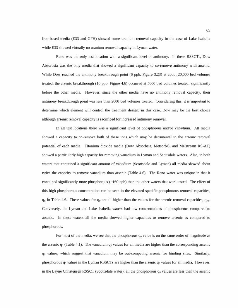
65

Iron-based media (E33 and GFH) showed some uranium removal capacity in the case of Lake Isabella

while E33 showed virtually no uranium removal capacity in Lyman water.

Reno was the only test location with a significant level of antimony. In these RSSCTs, Dow

Absorbsia was the only media that showed a significant capacity to co-remove antimony with arsenic.

While Dow reached the antimony breakthrough point (6 ppb, Figure 3.23) at about 20,000 bed volumes

treated, the arsenic breakthrough (10 ppb, Figure 4.6) occurred at 5000 bed volumes treated; significantly

before the other media. However, since the other media have no antimony removal capacity, their

antimony breakthrough point was less than 2000 bed volumes treated. Considering this, it is important to

determine which element will control the treatment design; in this case, Dow may be the best choice

although arsenic removal capacity is sacrificed for increased antimony removal.

In all test locations there was a significant level of phosphorous and/or vanadium. All media

showed a capacity to co-remove both of these ions which may be detrimental to the arsenic removal

potential of each media. Titanium dioxide media (Dow Absorbsia, MetsorbG, and Melstream RS-AT)

showed a particularly high capacity for removing vanadium in Lyman and Scottsdale waters. Also, in both

waters that contained a significant amount of vanadium (Scottsdale and Lyman) all media showed about

twice the capacity to remove vanadium than arsenic (Table 4.6). The Reno water was unique in that it

contained significantly more phosphorous (~160 ppb) than the other waters that were tested. The effect of

this high phosphorous concentration can be seen in the elevated specific phosphorous removal capacities,

qP, in Table 4.6. These values for qP are all higher than the values for the arsenic removal capacities, qAs.

Conversely, the Lyman and Lake Isabella waters had low concentrations of phosphorous compared to

arsenic. In these waters all the media showed higher capacities to remove arsenic as compared to

phosphorous.

For most of the media, we see that the phosphorous q0 value is on the same order of magnitude as

the arsenic q0 (Table 4.1). The vanadium q0 values for all media are higher than the corresponding arsenic

q0 values, which suggest that vanadium may be out-competing arsenic for binding sites. Similarly,

phosphorous q0 values in the Lyman RSSCTs are higher than the arsenic q0 values for all media. However,

in the Layne Christensen RSSCT (Scottsdale water), all the phosphorous q0 values are less than the arsenic

66

q0 values which could be explained by the low concentration of phosphorous in the Scottsdale groundwater

(~8 ppb). The No Data (ND) entries for some vanadium k values in the above tables can be explained by

incomplete vanadium breakthrough. Without a full breakthrough curve, or at the very least, a couple of

data points showing increased effluent concentration (signifying the start of breakthrough), the Thomas rate

constant, k, cannot be determined. Similarly, a definitive q0 value cannot be determined, but since q0 is

independent of the shape of the breakthrough curve, a minimum value can be estimated from the amount of

bed volumes treated.

Thomas Fit Parametersk = 0.00013 [mL/min.mg]

q0 = 75000 [mg/g]

0.00

10.00

20.00

30.00

40.00

50.00

60.00

0 10000 20000 30000 40000 50000

Bed Volumes Treated

Effl

uent

As

Con

c. [p

pb]

Experimental DataThomas Fit

Fig. 4.1. Thomas Fit Estimation of Experimental Data

67

0.00

10.00

20.00

30.00

40.00

50.00

60.00

0 10000 20000 30000 40000 50000

Bed Volumes Treated

Effl

uent

As

Con

c. [p

pb]

Experimental Datak = .00013k = .0002k = .00005

Fig. 4.2. Effect of Adjusting Thomas Rate Constant, k

0.00

10.00

20.00

30.00

40.00

50.00

60.00

0 10000 20000 30000 40000 50000

Bed Volumes Treated

Effl

uent

As

Con

c. [p

pb]

Experimental Dataq0 = 75000q0 = 90000q0 = 50000

Fig. 4.3. Effect of Adjusting the Maximum Solid Phase Concentration, q0

68

Lyman, NE MetsorbG (11.1 ml/min, ReSc#1000) Mn Analysis

0.00

5.00

10.00

15.00

20.00

25.00

30.00

35.00

40.00

0 20000 40000 60000

B ed V o lumes

Lyman, NE AsXnp (Solmetex) Manganese Analysis

0.0

10.0

20.0

30.0

40.0

50.0

60.0

70.0

80.0

0 20000 40000 60000

B ed V o lumes

Lyman, NE AsXnp (Solmetex) Uranium Analysis

0.0

10.0

20.0

30.0

40.0

50.0

60.0

70.0

80.0

90.0

0 20000 40000 60000

B ed V o lumes

Fig. 4.4. Examples of solute breakthrough abnormalities from Lyman RSSCTs. Data points represent observed data while the solid line represents the Thomas fit.

69

Lyman, NE MetsorbG (11.1 ml/min,

ReSc#1000) As Analysis

0.00

5.00

10.00

15.00

20.00

25.00

30.00

0 20000 40000 60000

B ed V o lumes

Lyman, NE AsXnp (Solmetex) Arsenic Analysis

0.0

5.0

10.0

15.0

20.0

25.0

0 20000 40000 60000

B ed V o lumes

Lyman, NE E33 Phosphate Analysis

0.0

10.0

20.0

30.0

40.0

50.0

60.0

0 20000 40000 60000

B ed V o lumes

GFH - Lake Isabella RSSCT, U Curve (pH~7.3)

0

10

20

30

40

50

60

70

0 10000 20000 30000 40000 50000 60000 70000 80000

B ed V o lumes

Fig. 4.5. Common examples of Thomas equation fit to various adsorbate breakthrough data

70

Inf luent C o nc. ~ 51 ppb

0.00

20.00

40.00

60.00

80.00

0 5000 10000 15000 20000 25000 30000 35000 40000 45000 50000

Bed Volumes Treated

Efflu

ent A

rsen

ic C

once

ntra

tion

[ppb

]

AsXnp Eng

Dow GFH(3EBCT)

GFH(6EBCT)

Fig. 4.6 Arsenic Removal Performance from Reno RSSCTs

Influent Concentration = 42 ppb

0.00

10.00

20.00

30.00

40.00

50.00

0 10000 20000 30000 40000 50000 60000 70000 80000

Bed Volumes Treated

Efflu

ent A

rsen

ic C

once

ntra

tion

[ppb

]

GFH As E33 As

AsXnp As MetsorbG As

Fig. 4.7. Comparative Arsenic Removal for Lake Isabella RSSCTs

71

Influent Concentration = 22 ppb

0.00

10.00

20.00

0 10000 20000 30000 40000 50000 60000

Bed Volumes Treated

Effl

uent

Ars

enic

Con

cent

ratio

n [p

pb] Dow E33

AsXnp MetsorbG

Fig. 4.8. Comparative Arsenic Removal for Lyman RSSCTs

E33 Normalized Data - Lyman pH~7.5

0

0.2

0.4

0.6

0.8

1

1.2

0 10000 20000 30000 40000 50000 60000

Bed Volumes Treated

Norm

aliz

ed C

onc

[%]

As P V

Fig. 4.9. Normalized As, P, and V breakthrough curves for E33 media with Lyman, NE water

72

Influent As concentration = 51 ppb

0.00

10.00

20.00

30.00

40.00

50.00

60.00

0 5000 10000 15000 20000 25000 30000 35000 40000 45000Englehard Bed Volumes Treated

Effl

uent

As

Con

c. [p

pb]

Experimental DataThomas Fit

Area used to calculate mass

of solute adsorbed

Fig. 4.10. Example of mass of solute removed per mass of media calculation

73

CHAPTER 5: CONCLUSIONS This study has shed some light on the characteristics of metals that compete or that can be co-removed with

arsenic during an adsorption treatment process. Phosphorous and vanadium were found to breakthrough at

similar times to arsenic which suggests they have similar adsorption kinetics. Uranium removal efficiency

was found to be sensitive to water chemistry. Antimony was only found in one water source and showed

some removal capacity in titanium dioxide media.

The Valley Vista RSSCTs proved to be successful experiments. The field and lab RSSCTs

compared very well to the first tank of the full-scale system. This contributes to the validation of using

RSSCTs as a method of predicting full-scale performance. Secondly, reducing the ReSc number for E33

media from 2000 to 500 for logistical purposes was found to be invalid. Finally, it was discovered that the

iron-based media out-performed AAFS50 in the RSSCTs, which could translate to increased performance

in the full-scale treatment system.

Rim Rock RSSCTs achieved three objectives. First and foremost, the RSSCT data matched well

with the full-scale E33 system data. Secondly, in agreement with the Valley Vista data, it was found that

the iron-based media remove arsenic for more bed volumes than the aluminum-based AAFS50. Finally, it

was again found that lowering the ReSc number from 2000 to 1000 for E33 column design is invalid.

For the Licking Valley School District site in Columbus, OH, the main objective was to compare

the capacities of various media to remove arsenite (As(III)). These field-conducted RSSCTs were found to

predict more bed volumes of treatment than was observed at the pilot-scale. Some factors that could have

influenced this include: pre-filtering of the RSSCT influent, possible differences between pilot- and small-

scale influent water chemistry, and the pilot-scale was operated at a loading rate below that which the

RSSCTs were scaled. However, the RSSCTs did predict the same order of media performance as the pilot-

scale where GFH > E33 > HIX > AAFS50. The high concentration of iron in the influent may have

affected the performance of the RSSCTs to remove arsenic as well as co-occurring metals.

The main goal of the Lyman tests was to evaluate the capacities of various media to co-remove

arsenic and uranium. It was found that ArsenXnp (HIX) media showed the only capacity to co-remove

74

uranium. Manufacturers of titanium-based media claim that their product will remove uranium in contrast

to these tests. However, Lyman water is high in alkalinity and it is suspected that the water quality played

a role in the inefficiency of the media to remove uranium. A secondary objective was to compare the

scaling of GTO and MetsorbG columns with lower ReSc numbers (1000). Unlike for E33 in previous tests,

lowering the ReSc number for titanium based media was found to be valid, enabling the use of smaller

columns to alleviate operational problems.

Lake Isabella, California was the second site to have levels of uranium in excess of the MCL along

with arsenic. Here the primary goal was to evaluate media ability to co-remove uranium with arsenic.

Unlike the Lyman RSSCTs, all media (iron- and titanium- based, and HIX) showed a capacity to remove

uranium in Lake Isabella water. HIX removed uranium for the longest number of bed volumes (> 50,000),

but its arsenic capacity was very low.

The main objective for the Reno, NV RSSCTs was to evaluate co-removal of antimony with

arsenic. The only media to show a potential for removing antimony was GTO, although there were

operational problems attributed to media loss experienced during the test. The secondary goal of these

RSSCTs was to evaluate the validity of comparing data on a bed volume basis. This was done by running

two GFH RSSCTs scaled to 3 and 6.2 minute EBCTs. The breakthrough data from these two columns

were nearly identical illustrating that comparing RSSCT data to full-scale data on a bed volume basis is

valid.

The objective of the RSSCTs conducted with Scottsdale groundwater was to compare new

adsorptive media (Next, Englehard ARM200, and Melstream) with commonly used commercial media

(E33 and GTO). It was found that Next removed arsenic for 10,000 bed volumes longer than E33. Batch

isotherms suggest that all the iron-based media (Next, ARM200, and E33) should perform similarly in the

RSSCTs. All media showed a capacity to remove phosphorous and vanadium with the titanium dioxide

media showing a particular affinity for vanadium removal.

This study also identified the potentials of commercially available adsorptive media to remove the

various solutes. Titanium dioxide media showed a capacity to remove phosphorous, vanadium and

antimony. There seems to be some removal capacity for uranium as well, but this may be highly sensitive

75

to water chemistry as was shown by the Lyman, NE RSSCT. ArsenXnp HIX resin proved to be the most

effective media at co-removing uranium. At the same time, ArsenXnp was found to be relatively poor at

removing phosphorous. The iron-based media (E33, GFH and ARM200) showed at least some capacity to

co-remove all solutes in this research. Uranium removal was observed in one out of two waters for these

media which indicates a sensitivity to water chemistry. The iron media were consistently the most efficient

at removing phosphorous.

Additionally, this research has raised some questions that are worthy of further attention. The

chromatographic-like breakthrough curve for uranium adsorption onto ArsenXnp HIX media for Lyman

water is very interesting for a couple of reasons. First, the ArsenXnp RSSCT produced an effluent with

twice the uranium concentration of the influent. This would suggest that there is a mechanism that is

displacing the uranium from the media. Second, the Lake Isabella ArsenXnp RSSCT outperformed the

Lyman ArsenXnp RSSCT for uranium removal, and this could be due to differences in the alkalinities of

Lyman and Lake Isabella groundwaters. Further research could lead to a better understanding of uranium

adsorption.

The data obtained for antimony could be viewed as somewhat inconclusive. Since only Reno

water contained significant levels of antimony, one must be careful when drawing conclusions. In this one

set of RSSCTs, titanium dioxide was the only media that showed any noticeable capacity to remove

antimony. However, if antimony adsorption kinetics are highly sensitive to water chemistry as was

observed with uranium, it may be found that iron-based media and ion exchange resin have an antimony

removal capacity in a water chemistry different than that of Reno.

Future work in adsorptive technologies for drinking water treatment could lead to some interesting

advancements. As mentioned above, the uranium “shedding” phenomenon experienced in this research

requires some attention. Identifying the mechanism that causes the release of adsorbed uranium on the ion

exchange resin could lead to developments that enhance the removal capacity for uranium. Another area of

research could investigate the capacity of commercially-available adsorption media to treat emerging

contaminants. For example, tungsten has been found in significant quantities in groundwater sources in

Nevada, and the potential health risks of tungsten exposure are not fully known. Similarly, vanadium is

76

currently on the EPA’s contaminant candidate list (CCL), and further research can expand our knowledge

on vanadium treatment of drinking water. Finally, as the realm of nanotechnology expands, it is interesting

to consider the potential impacts on drinking water treatment. The capacity to build adsorptive media,

starting from the nanoscale, may lead to an increased treatment capacity of common contaminants.

Additionally, there may be a potential to target specific contaminants with nano-engineered adsorptive

materials. Also, with the ever-increasing number of products containing nano-particles being

commercialized, these particles will inevitably be present in municipal drinking water systems. The

environmental fate and transport, as well as the drinking and wastewater treatment of nano-particles are

research topics that require future attention.

77

References Axe, L., and Trivedi, P. (2002). “Intraparticle surface diffusion of metal contaminants and their attenuation

in microporous amorphous Al, Fe, and Mn oxides.” Journal of Colloid and Interface Science, 247(2), 259-265.

Badruzzaman, M., Westerhoff, P., and Knappe, D. R. U. (2004). “Intraparticle diffusion and adsorption of

arsenate onto granular ferric hydroxide (GFH).” Water Research, 38(18), 4002-4012. Crittenden, J. C., Berrigan, J. K., and Hand, D. W. (1986). “Design of Rapid Small-Scale Adsorption Tests

For a Constant Diffusivity.” Journal Water Pollution Control Federation, 58(4), 312-319. Crittenden, J. C., Berrigan, J. K., Hand, D. W., and Lykins, B. (1987). “Design of Rapid Fixed-Bed

Adsorption Tests For Nonconstant Diffusivities.” Journal of Environmental Engineering-Asce, 113(2), 243-259.

Crittenden, J. C., Reddy, P. S., Arora, H., Trynoski, J., Hand, D. W., Perram, D. L., and Summers, R. S.

(1991). “Predicting GAC Performance With Rapid Small-Scale Column Tests.” Journal American Water Works Association, 83(1), 77-87.

Goldberg, S., and Johnston, C. T. (2001). “Mechanisms of arsenic adsorption on amorphous oxides

evaluated using macroscopic measurements, vibrational spectroscopy, and surface complexation modeling.” Journal of Colloid and Interface Science, 234(1), 204-216.

Lin, T. F., and Wu, J. K. (2001). “Adsorption of arsenite and arsenate within activated alumina grains:

Equilibrium and kinetics.” Water Research, 35(8), 2049-2057. McNeill, L. S., and Edwards, M. (1997). “Predicting As removal during metal hydroxide precipitation.”

Journal American Water Works Association, 89(1), 75-86. Meng, X. G., Bang, S., and Korfiatis, G. P. (2000). “Effects of silicate, sulfate, and carbonate on arsenic

removal by ferric chloride.” Water Research, 34(4), 1255-1261. Meng, X. G., Korfiatis, G. P., Bang, S. B., and Bang, K. W. (2002). “Combined effects of anions on arsenic

removal by iron hydroxides.” Toxicology Letters, 133(1), 103-111. Raven, K. P., Jain, A., and Loeppert, R. H. (1998). “Arsenite and arsenate adsorption on ferrihydrite:

Kinetics, equilibrium, and adsorption envelopes.” Environmental Science & Technology, 32(3), 344-349.

Reynolds, Tom D., Richards, Paul A., Unit Operations and Processes in Environmental Engineering, 1996,

pg. 364. Westerhoff, P., Highfield, D., Badruzzaman, M., and Yoon, Y. (2005). “Rapid small-scale column tests for

arsenate removal in iron oxide packed bed columns.” Journal of Environmental Engineering-Asce, 131(2), 262-271.

Wilkie, J. A., and Hering, J. G. (1996). “Adsorption of arsenic onto hydrous ferric oxide: Effects of

adsorbate/adsorbent ratios and co-occurring solutes.” Colloids and Surfaces a-Physicochemical and Engineering Aspects, 107, 97-110.

78

APPENDIX A

DATASETS FROM ALL RSSCT LOCATIONS

79

A.1 Dataset for Valley Vista, Arizona Site

Valley Vista Field Experiments (Routine Sampling)

Sample Location (influent/effluent) Influent pH

Influent Temperature (oC) Arsenic (ppb) Iron (ppb)

Manganese (ppb)

Silica (ppm)

Calcium (ppm)

Vanadium (ppb)

Phosphorous(ppb)

Aluminum (ppb)

Influent 7.62 20 39 3.49 0.202 18.0 39 14.8 17.8 7.44

Influent 7.99 18.2 40 4.1 0.192 19.0 41 15.2 19.7 5.59

Media Description

# Bed Volumes Treated

Sample Location (influent/effluent)

Raw water pH

Raw water Temperature (oC) Arsenic (ppb) Iron (ppb)

Manganese (ppb)

Silica (ppm)

Calcium (ppm)

Vanadium (ppb)

Phosphorous(ppb)

Aluminum (ppb)

126.5 Effluent 7.62 20 0 1.71 1.71 4.0 32 0.00 0.00 17.24091 Effluent 7.68 20 0 43.3 43.3 14.0 35 0.00 0.00 10.910559 Effluent 7.73 19.2 5.34 0.377 0.377 18.0 36 4.61 0.00 18.6713446 Effluent 7.51 21 26.9 0.367 0.367 17.0 39 13.5 0.00 38.8

AAFS-50 16672 Effluent 7.53 23 25 0.166 0.166 17.0 40 10.6 13.3 15.422677 Effluent 7.51 21 44 0.147 0.147 18.0 39 15.40 0.00 6.2626567 Effluent 7.78 21.1 37.8 0.104 0.104 17.0 38 14.90 9.80 15.730699 Effluent 7.9 20.9 38.2 0.110 0.110 18.0 41 15.6 10.9 6.2636864 Effluent 7.85 21.1 21.4 3.38 3.38 17.0 40 16.5 26.5 19.340674 Effluent 8.04 18.2 33.2 0.098 0.098 18.0 39 13.1 14.4 13.844452 Effluent 7.99 18.2 37.1 0.146 0.146 18.0 37 14.7 15.3 10.554561 Effluent 37.7 0.15 0.15 18.0 35 14.5 17.5 11.6358591 Effluent 7.85 12.3 38.6 0.14 0.19 18.0 42 12.98 16.84 10.564462 Effluent 38.6 0.12 0.13 19.0 41 13.0 17.8 11.9

149 Effluent 7.62 20 0 2.30 0.59 2.0 29 0.0 0 3.44241 Effluent 7.68 20 0 2.12 37 16.0 39 0.00 0.00 8.5

GFH 8813 Effluent 7.73 19.2 0 2.93 0.067 16.0 38 0.0000 0.00 3.9417323 Effluent 7.51 21 0 2.65 0.067 17.0 40 0 0.00 2.4822835 Effluent 7.53 23 0.19 3.30 0.129 18.0 41 0.0 8.2 19.128690 Effluent 7.51 21 0.76 1.02 0.065 18.0 39 0.00 0.00 n.d.37427 Effluent 7.78 21.1 3.9 12.49 0.344 17.0 36 0.00 7.8 5.2042827 Effluent 7.9 20.9 7.3 3.40 0.095 18.0 37 0.00 9.5 2.2848180 Effluent 7.85 21.1 9.56 2.02 0.138 17.0 39 0.00 0.00 3.0862506 Effluent 8.04 18.2 23.4 1.42 8.3 18.0 40 0.066 19.7 4.368216 Effluent 7.99 18.2 18.2 28.7 0.307 17.0 41 0.876 14.8 3.475579 Effluent 24 2.59 1.76 18.0 39 0.64 17.8 6.1

184 Effluent 7.62 20 0 1.97 0.066 7 26 0 0.00 7.755957 Effluent 7.68 20 0 1.318 0.037 18 38 0 0.00 2.6115374 Effluent 7.73 19.2 0.7 2.60 0.041 18 40 0 0.00 4.0

E33 19578 Effluent 7.51 21 0.22 1.397 0.031 18 39 0.000 0.00 3.5024276 Effluent 7.53 23 0.36 2.1 0.060 18 41 0.104 0.00 4.0133020 Effluent 7.51 21 3.84 7.86 0.128 18.00 39 6.12 10.45 11.838684 Effluent 7.78 21.1 6.8 2.18 0.088 17.0 40 9.4 13.5 5.1644700 Effluent 7.9 20.9 10.7 8.9 1.197 18 37 13.84 33.8 3.4453677 Effluent 7.85 21.1 40.5 170 1.38 17 39 13.79 25.959225 Effluent 8.04 18.2 20.6 1.86 0.050 18.0 37 16.3 22.6 2.1364726 Effluent 7.99 18.2 23.9 2.18 0.092 18.0 38 16.9 15.9 5.579445 Effluent 45 3.02 0.203 17.0 35 16.6 21.3 19.685312 Effluent 29.8 2.17 0.100 17.0 40 14.4 19.9 3.6093905 Effluent 28.9 1.53 0.53 17.0 41 12.9 19.3 8.1

80

A.1 Dataset for Valley Vista, Arizona Site (cont.)

Valley Vista Field Experiments (Weekly Sampling)

Media Description



Alkalinity (mg/L as CaCO3)

Sulfate (mg/L)

Chloride (mg/L)

Fluoride (mg/L)

Total Organic Carbon (mg/L)

126.5 Effluent 88.69 11.25 0.219 1.94091 Effluent10559 Effluent 127 10.25 11.77 0.25 1.613446 Effluent16672 Effluent 154 10.12 11.12 0.25 1.4

AAFS-50 22677 Effluent26567 Effluent30699 Effluent 157 10.12 11.12 0.24 1.636864 Effluent40674 Effluent 15844452 Effluent54561 Effluent 10.51 0.15 1.858591 Effluent 155 10.07 11.31 0.23 1.964462 Effluent 10.04 11.62 0.25 1.7

149 Effluent 2.14241 Effluent 19.38 12.33 0.538813 Effluent 108 10.16 11.34 0.24 1.717323 Effluent 10.15 11.38 0.24

GFH 22835 Effluent 145 1.7328690 Effluent37427 Effluent 10.15 11.38 0.2342827 Effluent 153 1.7848180 Effluent 10.08 10.81 0.2362506 Effluent 16168216 Effluent 10.05 11.34 0.2475579 Effluent 160 10.03 11.51 0.23 1.69

184 Effluent 10.06 12.11 0.246 1.835957 Effluent15374 Effluent 158 10.01 11.37 0.23 219578 Effluent24276 Effluent 155 10.02 11.38 0.23 1.8

E33 33020 Effluent 10.15 12.06 0.2438684 Effluent44700 Effluent 159 10.13 11.82 0.23 1.5653677 Effluent59225 Effluent 15864726 Effluent 10.02 11.27 0.23 2.0579445 Effluent85312 Effluent 15893905 Effluent 10 11.82 0.24 1.9

81

A.1 Dataset for Valley Vista, Arizona Site (cont.)

Valley Vista Lab Tests (Routine Sampling)

Media Description



Raw water pH

Raw Water Temperature (oC) Arsenic (ppb)

2159 Effluent 7.9 14.5 0.44276 Effluent 7.95 0.16478 Effluent 7.92 19.49103 Effluent 7.91 28.5

11135 Effluent 7.94 13.9 33AAFS-50 13189 Effluent 8.09 33.2

15348 Effluent 8.05 16.2 32.119138 Effluent 7.92 3623372 Effluent 7.85 15.2 34.929300 Effluent 7.95 36.836964 Effluent 8.01 14.2 37.847549 Effluent 38.551191 Effluent 41.557288 Effluent63385 Effluent69482 Effluent

3019 Effluent 7.9 14.5 0.35979 Effluent 7.95 0.79058 Effluent 7.92 0.6

12728 Effluent 7.91 0.515570 Effluent 7.94 13.9 0.9

GFH 18441 Effluent 8.09 0.621461 Effluent 8.05 16.2 0.826760 Effluent 7.92 2.232680 Effluent 7.85 15.2 440968 Effluent 7.95 10.651684 Effluent 8.01 14.2 20.466485 Effluent 24.371577 Effluent 27.580102 Effluent 31.488627 Effluent97153 Effluent

3019 Effluent 7.9 14.5 0.15979 Effluent 7.95 0.49058 Effluent 7.92 0.2

12728 Effluent 7.91 0.315570 Effluent 7.94 13.9 0.318441 Effluent 8.09 0.7

E33 21461 Effluent 8.05 16.2 0.926760 Effluent 7.92 1.732680 Effluent 7.85 15.2 3.940968 Effluent 7.95 11.251684 Effluent 8.01 14.2 1766485 Effluent 2071577 Effluent 22.580102 Effluent 25.688627 Effluent 29.197153 Effluent

82

A.2 Dataset for Rimrock, Arizona Site

Rimrock (Routine Sampling) 62 3 0.4 27 79 9 16 2

Description



Arsenic (ppb) Iron (ppb)

Manganese (ppb)

Silica (ppm) Calcium (ppm)

Vanadium (ppb)

Phosphorous (ppb)

Aluminium (ppb)

1637 Influent 63 3.16 0.173 26 78 9.5 23 2.52266270 Influent 60 3.43 0.168 27 81 9.1 23 1.8285940 Influent 61.818 3.6 0.9 29 77 8.72 2.355 2.405

Media Description



Raw Water pH

Raw water Temperature

(oC) Arsenic (ppb) Iron (ppb)Manganese

(ppb)Silica (ppm)

Calcium (ppm)

Vanadium (ppb)

Phosphorous (ppb)

Aluminium (ppb)

0AAFS-50 800

1637 Effluent 7.58 20 0.796 16.826 2.751 19 74 0.036 1.594 131.7198202 Effluent 19.5 46.862 1.619 0.786 19 79 6.885 5.493 21.9979911 Effluent 7.67 18.5 57.698 2.723 0.333 19 81 7.84 8.398 18.056

13670 Effluent 7.48 18.7 56.579 1.493 0.16 24 75 7.748 8.973 14.56617473 Effluent 7.61 19 64.672 3.638 0.163 24 76 8.145 10.481 21.51520250 Effluent 7.5 20.1 57.847 2.828 0.158 24 74 7.434 11.327 12.77722129 Effluent 7.65 19.5 57.908 7.526 0.225 25 77 7.757 12.919 13.41225761 Effluent 7.48 19.4 60.432 2.393 0.157 24 78 8.997 14.885 13.77929776 Effluent 7.45 18 65.723 4.491 0.146 26 81 8.967 16.933 15.14234134 Effluent 7.51 18 60.974 14.863 0.319 21 70 8.858 17.216 18.30636526 Effluent 7.66 18.5 67.329 3.44 0.52 24 79 8.226 18.522 57.94238577 Effluent 7.45 18.4 64.308 2.853 0.09 22 76 7.806 17.367 13.24242678 Effluent 63.416 2.457 0.09 25 75 8.588 18.872 10.09946352 Effluent 7.61 64.574 3.193 0.122 24 73 8.288 20.826 11.08852419 Effluent 7.51 18.5 61.472 2.97 0.139 24 79 8.67 20.001 9.60356093 Effluent 7.69 17 63.19 2.64 0.089 21 78 9.015 21.969 13.83460109 Effluent 66.197 2.814 0.075 26 81 8.204 21.713 8.49464552 Effluent 67.297 2.907 0.075 20 80 8.944 22.047 9.983

01000

GFH 2341 Effluent 7.58 20 0.038 14.299 0.724 17 55 0.019 1.559 67.00411727 Effluent 19.5 0.222 2.298 0.118 22 68 0.009 2.145 5.59414170 Effluent 7.67 18.5 0.072 92.793 1.22 23 71 0.19 2.077 7.17219545 Effluent 7.48 18.7 0.07 1.524 0.201 23 80 0.008 1.486 2.65724982 Effluent 7.61 19 0.165 4.88 0.269 20 78 0.018 4.237 4.15128952 Effluent 7.5 20.1 0.465 2.229 0.231 23 76 0.012 1.825 3.14631640 Effluent 7.65 19.5 0.903 2.697 0.226 23 79 0.012 2.258 2.35436831 Effluent 7.48 19.4 2.581 4.235 0.223 22 75 0.01 4.136 3.3242573 Effluent 7.45 18 5.696 5.724 0.167 24 79 0.015 5.957 3.30848803 Effluent 7.51 18 7.666 2.327 0.116 22 81 0.01 7.451 2.11652224 Effluent 7.66 18.5 5.951 3.583 0.122 22 75 0.012 7.19 2.31855156 Effluent 7.45 18.4 20.43 4.049 0.115 23 79 0.017 13.679 3.76461020 Effluent 19.209 4.039 0.124 23 76 0.014 13.394 2.5766272 Effluent 7.61 26.137 2.759 0.077 24 77 0.02 16.129 1.82374946 Effluent 7.51 18.5 30.803 3.634 0.094 23 79 0.052 17.429 3.8280199 Effluent 7.69 17 36.221 2.891 0.069 22 74 0.091 18.828 2.285941 Effluent 39.94 2.819 0.065 23 79 0.182 20.077 2.72892293 Effluent 61.337 3.181 0.074 23 81 0.43 24.767 4.515

01000

E33 2341 Effluent 7.58 20 nd 12.4 0.534 25 61 nd 0.909 56.03711727 Effluent 19.5 0.085 1.584 0.269 23 74 0.011 0.768 2.92614170 Effluent 7.67 18.5 0.17 2.2 0.203 25 73 nd 1.53 3.76219545 Effluent 7.48 18.7 0.185 1.4 0.121 25 79 nd 1.138 1.7124982 Effluent 7.61 19 0.48 138 1.393 23 81 0.31 1.926 3.42828952 Effluent 7.5 20.1 0.52 8.6 0.207 25 78 0.093 3.953 2.62831640 Effluent 7.65 19.5 1.0 2.96 0.265 23 75 0.22 2.44 6.33736831 Effluent 7.48 19.4 2.9 8.9 0.21 23 79 1.33 5.307 4.57542573 Effluent 7.45 18 9.55 3.5 0.162 24 76 4.8 13.57 2.98948803 Effluent 7.51 18 13.4 133 1.761 26 77 7.4 19.227 2.47152224 Effluent 7.66 18.5 27.0 3.0 0.104 22 79 7.8 26.891 3.33955156 Effluent 7.45 18.4 35 2.9 0.148 24 80 8.0 26.847 6.07961020 Effluent 30.6 3.5 0.171 25 81 8.1 23.416 10.93266272 Effluent 7.61 42 4.2 0.155 23 78 8.7 27.713 4.59274946 Effluent 7.51 18.5 41 3.9 0.159 22 77 9.0 24.687 2.41280199 Effluent 7.69 17 50 2.8 0.125 25 80 9.7 28.214 1.54685941 Effluent 47.598 2.742 0.102 24 74 7.716 28.348 1.82592293 Effluent 66.443 3.16 0.091 25 73 8.18 28.358 3.142

83

A.2 Dataset for Rimrock, Arizona Site (cont.)

Rimrock (Weekly Sampling)

Description




Sulfate (mg/L)

Chloride (mg/L)

Fluoride (mg/L)


1637 Influent 365 10.5 32 0.145 1.6536831 Influent 370 11.2 31.9 0.123 1.62

367.5 10.9 32.0 0.1 1.6

Media Description




Sulfate (mg/L)

Chloride (mg/L)

Fluoride (mg/L)


1637 Effluent 341 10.63 30.57 0.15 1.618202 Effluent9911 Effluent 362 11.58 33.91 0.15113670 Effluent17473 Effluent

AAFS 50 20250 Effluent 36822129 Effluent 10.34 30.83 0.11425761 Effluent29776 Effluent34134 Effluent 368 1.4536526 Effluent 11.56 32.4 0.1138577 Effluent42678 Effluent46352 Effluent 11.46 32.5 0.11252419 Effluent 36956093 Effluent 10.82 31.23 0.11460109 Effluent64552 Effluent 372 10.45 31.23 0.115 1.6

2341 Effluent 325 10.66 32.2 0.126 1.6911727 Effluent14170 Effluent 361 12.9 34.12 0.12119545 Effluent

GFH 24982 Effluent 13.91 35.99 0.1128952 Effluent 36731640 Effluent36831 Effluent 10.92 31.66 0.126 1.5942573 Effluent48803 Effluent 37152224 Effluent55156 Effluent61020 Effluent 10.31 30.97 0.12366272 Effluent74946 Effluent 36980199 Effluent 10.35 31.65 0.1485941 Effluent92293 Effluent 370 11.26 32.3 0.114 1.55

2341 Effluent 344 10.51 31.99 0.145 1.5111727 Effluent14170 Effluent 366 10.81 31.44 0.12519545 Effluent24982 Effluent 10.39 31.04 0.11728952 Effluent 366

E33 31640 Effluent36831 Effluent 10.33 30.62 0.113 1.4942573 Effluent48803 Effluent 36952224 Effluent55156 Effluent61020 Effluent 10.74 31.45 0.11566272 Effluent74946 Effluent 37280199 Effluent 10.33 30.65 0.1185941 Effluent92293 Effluent 374 13.07 34.69 0.133 1.62

84

A.3 Dataset for Licking Valley School District, Ohio Site

Licking Valley School District, Newark, OH Routine Sampling

Description


Sample Location (influent/effluent) pH Temperature (oC) Arsenic (ppb) Iron (ppb)

Manganese (ppb)

Silica (ppm)

Calcium (ppm)

Vanadium (ppb)

Phosphorous (ppb)

Aluminium (ppb)

1820 Influent 8.11 17.5 66 1376 184 6 56 0.000 45.0 1.946921 Influent 7.92 17.6 66 1418 183 5 58 0.000 48 3.1217063 Influent 8.14 18.3 65 1464 182 7 56 0.018 60 10.4

8.06 17.80 65.58 1419.73 183.17 6.00 56.67 0.01 51.15 5.16

Media Description


Sample Location (influent/effluent) pH Arsenic (ppb) Iron (ppb)

Manganese (ppb)


Vanadium (ppb)

Phosphorous (ppb)

Aluminium (ppb)

0 0 0 05001351 Effluent 7.56 10.3 1.898 138 3 54 0 1.14 66.12067 Effluent 7.77 16 7.88 159 4 56 0 1.2 69.63657 Effluent 12.5 2.28 147 5 55 0 1.05 665127 Effluent 22 2.65 170 4 52 0 0.8 58

AAFS-50 5783 Effluent 24 2.53 173 3 53 0 1.0 567214 Effluent 8.1 27 2.5 195 1 55 0 1.0 517512 Effluent 30 21.3 184 2 56 0 0.98 53.28864 Effluent 39 460 198 4 51 0.78 1.6 549420 Effluent 39 204 195 5 57 0.000 1.72 4910931 Effluent 41 342 190 6 55 0.000 0.9 5112640 Effluent 8.14 46 510 184 4 54 0.018 1.5 5714840 Effluent 52 520 171 5 53 bdl 2.5 2.217238 Effluent 47.8 644 175 6 54 bdl 2.5 3.8

0 0 0 09001824 Effluent 7.1 0 4.31 16.0 2 46 0 1.9 2.62790 Effluent 7.56 0.03 13.6 94 5 52 0 2.8 1.88

GFH 4936 Effluent 0 5.42 104 4 55 0 1.3 5.76921 Effluent 0.028 9.8 165 7 56 0 1.37 5.67807 Effluent 0 3.0 178 8 57 0 1.17 2.89739 Effluent 7.9 0.048 2.0 182 3 52 0 2.3 2.010141 Effluent 0 5.0 202 4 51 0 1.3 2.111965 Effluent 0 2.27 184 8 49 0 1.67 1.6212717 Effluent 0.03 5.5 183.0 5 50 0 1.0 2.6914756 Effluent 0 1.96 176 6 48 0 0.9 3.817063 Effluent 8.1 0.042 8.1 182 4 51 0 1.6 2.020032 Effluent 0.26 17.5 174 3 50 bdl 9.1 6.123269 Effluent 0.4 25.8 174 6 56 bdl 2.5 3.2

0 0 0 09001824 Effluent 7.5 0.0 2.2 35.9 5 49 0.000 1.20 2.112790 Effluent 7.62 0.04 2.3 119 4 51 0.000 1.5 2.32

E33 4936 Effluent 0.06 4.28 214 6 56 0.000 1.6 8.36921 Effluent 0.31 2.5 166 8 55 0.000 0.9 3.317807 Effluent 1.1 3.5 173 7 57 0.000 1.9 15.79739 Effluent 8.05 5.2 2.5 169.9 4 54 0.000 0.9 2.0110141 Effluent 8.6 4.84 177 3 53 0.000 0.80 2.0511965 Effluent 15 4.82 172 4 55 0.000 1.9 4.0312717 Effluent 16.9 3.03 172 3 54 0.000 1.2 2.4014756 Effluent 23.2 9.2 163 5 57 0.000 1.1 4.317063 Effluent 8.1 26.7 33.9 176 6 55 0.0180 1.72 5.1820032 Effluent 27 27 170 8 51 0.018 3.2 3.3423269 Effluent 37.8 170 199.0 7 52 bdl 2.5 6.7

0 0 0 05001195 Effluent 7.72 0.034 2.91 147 3 50 0.000 2.3 1.651827 Effluent 7.78 0.044 8.1 161 4 51 0.000 1.1 2.1

ArsenXnp 3233 Effluent 0.066 4.8 150 7 56 0.000 47 9.94534 Effluent 0.228 9.0 162 6 54 0.000 1.9 3.75113 Effluent 0.942 5.0 166 4 57 0.000 0.95 2.36379 Effluent 8.1 7.434 6.3 176 3 51 0.000 1.17 7.86642 Effluent 11.724 9.5 176 1 52 0.000 2.5 5.087837 Effluent 16.868 464 168 4 53 0.034 1.7 3.38329 Effluent 25.71 618 178 3 55 0.000 2.5 2.99665 Effluent 43.54 667 175 5 54 0.000 1.4 7.211176 Effluent 7.9 55.906 560 185 0 51 0.000 11.3 10.213121 Effluent 46.0 512 175 4 52 bdl 2.6 4915242 Effluent 58 1541 175 6 51 bdl 2.9 63

85

A.3 Dataset for Licking Valley School District, Ohio Site (cont.)

Licking Valley School District, Newark, OH (Weekly Sampling)

Description




Sulfate (mg/L)

Chloride (mg/L)

Fluoride (mg/L)


1820 Influent 525 7.49 9.18 0.0117063 Influent 485 7.5 7.84 0.01

505 7.495 8.51 0.01

Media Description




Sulfate (mg/L)

Chloride (mg/L)

Fluoride (mg/L)


1351 Effluent 475 8.93 9.32 0.012067 Effluent3657 Effluent5127 Effluent 7.92 8.85 0.01

AAFS-50 5783 Effluent7214 Effluent7512 Effluent8864 Effluent9420 Effluent10931 Effluent 8.49 8.46 0.0112640 Effluent 50514840 Effluent17238 Effluent

1824 Effluent 460 7.47 8.92 0.012790 Effluent

GFH 4936 Effluent6921 Effluent 7.46 9.11 0.017807 Effluent9739 Effluent10141 Effluent11965 Effluent12717 Effluent14756 Effluent 7.66 9.02 0.0117063 Effluent 51520032 Effluent23269 Effluent

1824 Effluent 492 7.43 8.8 0.012790 Effluent

E33 4936 Effluent6921 Effluent 7.43 8.85 0.017807 Effluent9739 Effluent10141 Effluent11965 Effluent12717 Effluent14756 Effluent 7.44 9.05 0.0117063 Effluent 51020032 Effluent23269 Effluent

1195 Effluent 7.43 8.77 0.041827 Effluent

ArsenXnp 3233 Effluent4534 Effluent 14.6 42.57 0.25113 Effluent6379 Effluent6642 Effluent7837 Effluent8329 Effluent9665 Effluent 8.99 8.85 0.0111176 Effluent13121 Effluent15242 Effluent

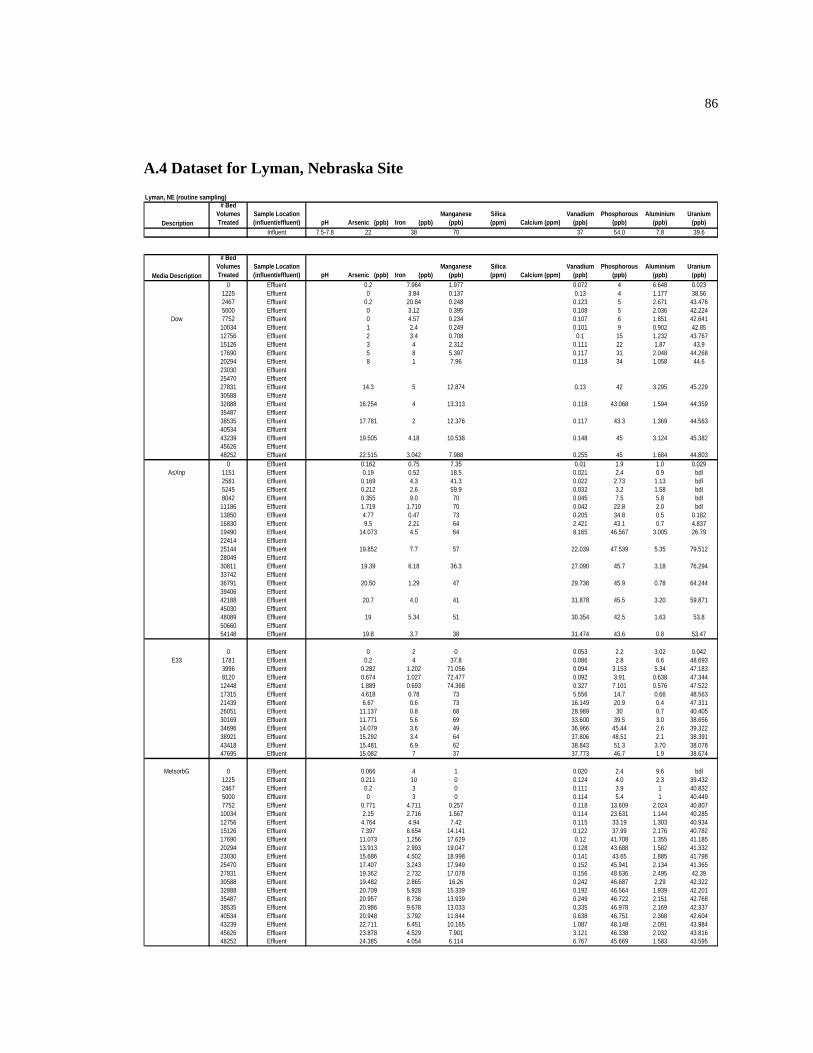
86

A.4 Dataset for Lyman, Nebraska Site

Lyman, NE (routine sampling)

Description



Manganese (ppb)


Vanadium (ppb)

Phosphorous (ppb)

Aluminium (ppb)

Uranium (ppb)

Influent 7.5-7.8 22 38 70 37 54.0 7.8 39.6

Media Description



Manganese (ppb)


Vanadium (ppb)

Phosphorous (ppb)

Aluminium (ppb)

Uranium (ppb)

0 Effluent 0.2 7.964 1.977 0.072 4 6.648 0.0231225 Effluent 0 3.84 0.137 0.13 4 1.177 38.562467 Effluent 0.2 20.84 0.248 0.123 5 2.671 43.4765000 Effluent 0 3.12 0.395 0.108 5 2.036 42.224

Dow 7752 Effluent 0 4.57 0.234 0.107 6 1.851 42.64110034 Effluent 1 2.4 0.249 0.101 9 0.902 42.8512756 Effluent 2 3.4 0.708 0.1 15 1.232 43.76715126 Effluent 3 4 2.312 0.111 22 1.87 43.917690 Effluent 5 8 5.397 0.117 31 2.048 44.26820294 Effluent 8 1 7.96 0.118 34 1.058 44.623030 Effluent25470 Effluent27831 Effluent 14.3 5 12.874 0.13 42 3.295 45.22930588 Effluent32888 Effluent 16.254 4 13.313 0.118 43.068 1.594 44.35935487 Effluent38535 Effluent 17.781 2 12.376 0.117 43.3 1.369 44.56340534 Effluent43239 Effluent 19.505 4.18 10.538 0.148 45 3.124 45.38245626 Effluent48252 Effluent 22.515 3.042 7.988 0.255 45 1.684 44.803

0 Effluent 0.162 0.75 7.35 0.01 1.9 1.0 0.029AsXnp 1151 Effluent 0.19 0.52 18.5 0.021 2.4 0.9 bdl

2581 Effluent 0.169 4.3 41.3 0.022 2.73 1.13 bdl5245 Effluent 0.212 2.6 59.9 0.032 3.2 1.58 bdl8042 Effluent 0.355 9.0 70 0.045 7.5 5.8 bdl11186 Effluent 1.719 1.710 70 0.042 22.8 2.0 bdl13850 Effluent 4.77 0.47 73 0.205 34.8 0.5 0.18216830 Effluent 9.5 2.21 64 2.421 43.1 0.7 4.83719490 Effluent 14.073 4.5 64 8.165 46.567 3.005 26.7922414 Effluent25144 Effluent 19.852 7.7 57 22.039 47.539 5.35 79.51228049 Effluent30811 Effluent 19.39 6.18 36.3 27.090 45.7 3.18 76.29433742 Effluent36791 Effluent 20.50 1.29 47 29.736 45.9 0.78 64.24439406 Effluent42188 Effluent 20.7 4.0 41 31.878 45.5 3.20 59.87145030 Effluent48089 Effluent 19 5.34 51 30.354 42.5 1.63 53.850660 Effluent54148 Effluent 19.8 3.7 38 31.474 43.6 0.8 53.47

0 Effluent 0 2 0 0.053 2.2 3.02 0.042E33 1781 Effluent 0.2 4 37.8 0.086 2.8 0.6 48.693

3996 Effluent 0.282 1.202 71.056 0.094 3.153 5.34 47.1838120 Effluent 0.674 1.027 72.477 0.092 3.91 0.638 47.34412448 Effluent 1.889 0.693 74.368 0.327 7.101 0.576 47.52217315 Effluent 4.618 0.78 73 5.556 14.7 0.66 48.56321439 Effluent 6.67 0.6 73 16.149 20.9 0.4 47.31126051 Effluent 11.137 0.8 68 28.989 30 0.7 40.40530169 Effluent 11.771 5.6 69 33.600 39.5 3.0 38.65634696 Effluent 14.079 3.6 49 36.966 45.44 2.6 39.32238921 Effluent 15.292 3.4 64 37.806 48.51 2.1 38.39143418 Effluent 15.481 6.9 62 38.843 51.3 3.70 38.07847695 Effluent 15.082 7 37 37.773 46.7 1.9 38.674

MetsorbG 0 Effluent 0.066 4 1 0.020 2.4 9.6 bdl1225 Effluent 0.211 10 0 0.124 4.0 2.3 39.4322467 Effluent 0.2 3 0 0.111 3.9 1 40.8325000 Effluent 0 3 0 0.114 5.4 1 40.4497752 Effluent 0.771 4.711 0.257 0.118 13.609 2.024 40.80710034 Effluent 2.15 2.716 1.567 0.114 23.631 1.144 40.28512756 Effluent 4.764 4.94 7.42 0.115 33.19 1.303 40.93415126 Effluent 7.397 6.654 14.141 0.122 37.99 2.176 40.78217690 Effluent 11.073 1.256 17.629 0.12 41.708 1.355 41.18520294 Effluent 13.913 2.993 19.047 0.128 43.688 1.582 41.33223030 Effluent 15.686 4.502 18.998 0.141 43.65 1.885 41.79825470 Effluent 17.407 3.243 17.949 0.152 45.941 2.134 41.36527831 Effluent 19.362 2.732 17.078 0.156 48.636 2.495 42.3930588 Effluent 19.482 2.865 16.26 0.242 46.687 2.29 42.32232888 Effluent 20.709 5.928 15.339 0.192 46.564 1.939 42.20135487 Effluent 20.957 8.736 13.939 0.249 46.722 2.151 42.76838535 Effluent 20.986 9.678 13.033 0.335 46.978 2.169 42.33740534 Effluent 20.948 3.792 11.844 0.638 46.751 2.368 42.60443239 Effluent 22.711 6.451 10.165 1.087 48.148 2.091 43.98445626 Effluent 23.878 4.529 7.901 3.121 46.338 2.032 43.81648252 Effluent 24.385 4.054 6.114 6.767 45.669 1.583 43.595

87

A.4 Dataset for Lyman, Nebraska Site (cont.)

Lyman, NE (Weekly Sampling)

Description




Sulfate (mg/L)

Chloride (mg/L)

Fluoride (mg/L)


Influent 330 475.8125 36.23906 0.091463 4.428Influent 375 478.176 36.44108 0.094729 3.716Influent 317 478.2136 36.65697 0.086869 3.838Influent 333 473.977 36.1651 0.094533 3.649Influent 357 474.1268 36.55263 0.091383 3.463

Ave 352.5 476.0612 36.41097 0.091795 3.8188

Media Description




Sulfate (mg/L)

Chloride (mg/L)

Fluoride (mg/L)


24500 Effluent 333 476.0822 36.38797 0.084376 3.2Dow 55000 Effluent 333 478.0382 36.52921 0.092114 3.5

5000 Effluent 330 476.775 36.33351 0.090132 5.220000 Effluent 330 475.7192 36.33919 0.094604 4.145000 Effluent 400 469.4735 36.27776 0.090555 6.6

AsXnp 13500 Effluent 333 479.095 36.64707 0.08851 3.430000 Effluent 333 483.9027 37.23099 0.103368 3.745000 Effluent 330 477.3052 36.07318 0.093272 3.8

E33 21000 Effluent 337 478.4043 36.54171 0.090646 4.343000 Effluent 350 476.0908 36.62622 0.104366 3.8

MetsorbG 24500 Effluent 350 478.2772 36.44004 0.0911 3.555000 Effluent 343 480.9583 36.67644 0.091639 3.85000 Effluent 330 481.3254 36.80731 0.088541 3.6

20000 Effluent 333 476.4478 36.2675 0.091872 3.645000 Effluent 410 474.4011 36.65131 0.090597 4.0

88

A.5 Dataset for Lake Isabella, California Site Lake Isabella (Routine Sampling)

Media Description



Manganese (ppb)

Silica (ppm)

Calcium (ppm)

Vanadium (ppb)

Uranium (ppb)

Dow(ReSc=1000) 083.75 Effluent 5.05 18 0.2 1.3 2.385 0 13.2 0.467 0.0090

3601.25 Effluent 18 0.087 0.8 0.082 0.228 0.605695 Effluent 7.71 18 0.3 0.84 0.126 8.6 25.3 0.116 0.963

8929.84375 Effluent 7.76 18 1.0 0.8 0.041 0.077 2.7413944.375 Effluent 18 5.8 0.7 0.045 8.5 25.4 0.054 8.017315.3125 Effluent 7.74 17 10.2 0.9 0.028 0.122 10.520807.6875 Effluent 7.93 17 9.3 25.3

23104.53125 Effluent 16 23 3.1 0.03 0.039 24.627051.25 Effluent 7.9 14

30348.90625 Effluent 14 19 11 0.077 0.07 20.535300.625 Effluent 7.74 14 10.1 2538780.4375 Effluent 14 27 12 0.068 0.018 28.641791.25 Effluent 7.23 14 11 25

44890 Effluent 14 33 11.1 0.071 0.02 33.047810.78125 Effluent 1454232.3125 Effluent 14 34 11.4 0.079 0.019 37.3

56950 Effluent 7.78 1460174.375 Effluent 14 35 11.3 0.111 0.019 39.8

62990.46875 Effluent 14 34 11.0 0.164 0.018 41.3

Dow(ReSc=2000) 083.75 Effluent 5.87 18 0.055 4.3 1.016 0.2 15.60 0.014 0.013576.125 Effluent 7.83 17

5872.96875 Effluent 17 1.765 3.2 0.029 8.8 25.300 0.018 89819.6875 Effluent 7.89 16

13117.34375 Effluent 14 8.503 11 0.06 8.2 24.800 0.01 1218069.0625 Effluent 7.76 1421548.875 Effluent 14 21.208 10.8 0.065 7.4 24.800 0.01 2624559.6875 Effluent 7.73 1427658.4375 Effluent 14 27.499 11.5 0.062 6.5 24.700 0.011 31.0

30579.21875 Effluent 14 5.8 24.737000.75 Effluent 14 27.305 11.1 0.071 0.013 37.429

39718.4375 Effluent 7.82 14 29.225 11 0.064 0.014 38.5442942.8125 Effluent 14 33.17 16 0.21 0.29 46.73

45758.90625 Effluent 14 5.366 21.6 1.391 1.064 371.1

AsXnp, Lake Isabella 036.48290094 Effluent 5.01 18 bdl bdl 0.9 30 bdl bdl1525.648585 Effluent 7.16 183062.352594 Effluent 7.32 18 bdl bdl 3.4 bdl bdl6478.478774 Effluent 7.32 189203.64092 Effluent 7.39 18 bdl bdl 3.5 6.6 30 bdl bdl10729.2895 Effluent 18

12691.62736 Effluent 18 bdl bdl 3.7 bdl bdl14294.66392 Effluent 7.26 1815820.3125 Effluent 18 0.2 2.22 3.9 7.2 27.7 0.028 0.0230

19366.89269 Effluent 1820474.64623 Effluent 7.33 18 0.05 3.5 2.9 7.3 27.4 bdl bdl22171.65389 Effluent 1823680.71934 Effluent 18 0.5 1.9 3.7 7.3 26.9 bdl bdl26538.54658 Effluent 1830396.88974 Effluent 18 18.8 2.5 2.8 1.38 bdl31557.70932 Effluent 7.46 1833359.74351 Effluent 18 29 3.3 3.2 7 27.4 0.14 0.012035161.77771 Effluent 1836549.23349 Effluent 18 33 2.9 3.1 0.009 0.00938284.93514 Effluent 1840040.53656 Effluent 18 43 1.7 2.2 bdl 0.007042760.17099 Effluent 7.66 1846049.15979 Effluent 7.6 18 49 3.3 7.4 25.9 0.03 bdl47919.73762 Effluent 18

49218.75 Effluent 7.7 18 35.9 1.2 0.34 bdl50926.81309 Effluent 18 42.3 0.9 bdl bdl

GFH 068.39622642 Effluent 7 18 0.04 1.14 0.5 0 21.6 0.0140 0.0172371.639151 Effluent 7.14 184743.278302 Effluent 7.3 18 0.07 3.0 0.66 0.08 0.02110026.88679 Effluent 7.32 1814241.80425 Effluent 7.34 18 0.06 3.4 1.0 7 30.2 bdl 15.616601.47406 Effluent 1819636.5566 Effluent 18 0.07 2.5 0.84 bdl 23.8

22115.91981 Effluent 7.22 1824467.04009 Effluent 18 0.08 3.1 1.0 6.9 27.7 0.009 29.129955.83726 Effluent 1831670.87264 Effluent 7.33 18 0.8 2.6 1.0 7.7 27.5 0.011 37.834298.99764 Effluent 1836633.01887 Effluent 18 2.4 2.7 1.0 7.4 26.7 0.010 38.8

41053.125 Effluent 1847020.69575 Effluent 18 8.7 3.1 0.8 0.012 4748807.54717 Effluent 7.45 1851603.24292 Effluent 18 12 1.6 7 27 0.009 48.954381.83962 Effluent 1856536.32075 Effluent 18 15 2.11 0.65 0.010 53.159220.87264 Effluent 1861936.20283 Effluent 18 22 3.4 0.41 0.009 61.166137.44104 Effluent 7.67 1871229.54009 Effluent 7.59 18 33 2.2 7.6 25.6 bdl 56.974122.70047 Effluent 18 40.9 1.0 bdl 62.9

E33 068.39622642 Effluent 7.32 18 0.26 1.04 0.15 4.1 37.3 0.045 0.01802371.639151 Effluent 7.17 184743.278302 Effluent 7.3 18 0.12 2.36 0.33 bdl 0.020010026.88679 Effluent 7.3 1814241.80425 Effluent 7.36 18 0.17 2.5 0.98 8.2 30.3 bdl 36.516601.47406 Effluent 1819636.5566 Effluent 18 0.2 2.6 1.20 0.026 60

22115.91981 Effluent 7.22 1824467.04009 Effluent 18 0.2 3.0 1.09 8.7 28 0.008 6729955.83726 Effluent 1831670.87264 Effluent 7.31 18 1.4 2.3 0.9 8.7 27.8 0.04 68.534298.99764 Effluent 1836633.01887 Effluent 18 5.2 2.36 0.99 8.5 27.3 0.012 64

41053.125 Effluent 1847020.69575 Effluent 18 17 1.3 0.77 0.010 6248807.54717 Effluent 7.46 1851603.24292 Effluent 18 17.6 2.8 8.3 27.6 0.018 5854381.83962 Effluent 1856536.32075 Effluent 18 22 2.6 0.71 0.008 6059220.87264 Effluent 1861936.20283 Effluent 18 27 1.6 0.50 bdl 63.066137.44104 Effluent 7.7 1871229.54009 Effluent 7.61 18 33 2.2 8.4 26.2 bdl 57.374122.70047 Effluent 18 36.5 2.03 bdl 58

Metsorb G 03167.84375 Effluent 6.94 18 0.05 0.74 0.15 0 15.8 0.0080 0.0166375.46875 Effluent 7.81 18 0.07 1.3 0.08 6.5 26.1 0.010 1.9269411.40625 Effluent 18 0.3 0.61 0.030 7.6 25.8 bdl 10.1

12928.90625 Effluent 18 2.5 0.61 0.0470 8.6 25.9 0.010 20.215399.53125 Effluent 7.71 18 3.5 0.61 0.033 9.4 25.2 bdl 17.3

18634.375 Effluent 7.77 18 7.2 0.41 0.029 9.7 25.1 bdl 23.6523648.90625 Effluent 18 11.8 0.76 0.04 bdl 22.8

89

A.5 Dataset for Lake Isabella, California Site (cont.)

Lake Isabella (Weekly Sampling)

Media Description




Sulfate (mg/L)

Chloride (mg/L)

Fluoride (mg/L)


Feed 9/23,1510 Influent 143.3 39.59662 12.629925 1.64205 0.409Feed 10/3, 1240 Influent 76.7 39.360564 12.183485 1.33855 0.337Feed 10/10. 1220 Influent 83.3 39.341324 12.088885 1.33653 0.301Feed 10/17, 1400 Influent 66.7 39.427124 12.29541 1.33547 0.507Feed 10/20, 1140 Influent 38.918788 12.162595 1.283795 0.324Feed 10/25, 1050 Influent 60 38.729532 11.98409 1.237105Feed 10/31/2005 Influent 93.3

GFH 9/23, 1510 7205 Effluent 110 39.359484 12.280895 1.709425 0.335GFH 10/3, 1240 ~30000 Effluent 83.3 39.15406 12.000455 1.33848 0.259GFH 10/10, 1220 ~48800 Effluent 76.7 38.803676 11.06399 1.470935 0.256GFH 10/17, 1400 ~66000 Effluent 76.7 39.048508 11.071825 1.47864 0.288GFH 10/20, 1930 ~74000 Effluent 56.7 39.14338 12.095475 1.274145

E33 9/23, 1510 ~7200 Effluent 116.7 39.316972 12.285055 1.41291 0.46E33 10/3, 1240 ~30000 Effluent 76.7 39.01706 12.18136 1.33504 0.277E33 10/10, 1220 ~48800 Effluent 90 39.007212 11.025135 1.47388 0.334E33 10/17, 1400 ~66000 Effluent 73.3 39.304436 12.046485 1.3177 0.263E33 10/20, 1930 ~74000 Effluent 66.7 38.984028 12.161485 1.267

AsXnp 9/23, 1510 ~4600 Effluent 123.3 39.711652 12.297305 1.90309 0.801AsXnp 10/3, 1240 ~20000 Effluent 76.7 38.995132 12.046265 1.33954 0.245AsXnp 10/10, 1220 ~31500 Effluent 76.7 39.035036 11.87721 1.35133 0.255AsXnp 10/17, 1400 ~42800 Effluent 76.7 39.836796 11.176225 1.49823 0.742AsXnp 10/20, 1930 ~48000 Effluent 63.3 38.975764 12.08343 1.31732

Dow (1000) 10/20, 1945 ~3600 Effluent 73.3 38.873572 11.894825 1.288225Dow (1000) 10/25, 1140 ~17300 Effluent 73.3 38.767188 12.061415 1.25724 0.36Dow (1000) 10/31, 1050 ~35300 Effluent 80 38.784748 12.15963 1.23431Dow (1000) 11/7 ~56950 0.302Dow (1000) 11/9 ~62990 0.36

Dow (2000) 10/25, 1140 ~84 Effluent 10* 78.0641 12.249355 1.1905 0.584 *Sample taken at very beginning of testDow (2000) 10/31, 1050 ~18100 Effluent 83.3 38.86914 12.07592 1.246245Dow (2000) 11/7 ~39720 0.313Dow (2000) 11/9 ~45750 0.291

MetsG 10/10, 1220 Effluent 83.3 (2) 39.180564 11.9133 1.313585 0.323* *This value is for one of the failed columnsMetsG 10/17, 1440 ~3200 Effluent 53.3 (3) 40.923004 12.050225 0.919505 0.442MetsG 10/20, 1945 ~13000 Effluent 73.3 (3) 38.667716 11.919305 1.268155

(#) - Denotes trial of MetsorbG. Had problems with MetsG columns (backpressure)

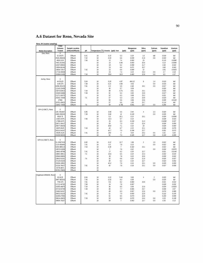
90

A.6 Dataset for Reno, Nevada Site

Reno, NV (routine sampling)

Media Description



Manganese (ppb)

Silica (ppm)

Calcium (ppm)

Vanadium (ppb)

Uranium (ppb)

Dow, Reno 052.34375 Effluent 6.41 18 0.10 5.3 0.29 1.6 bdl 0.018 bdl

2526.458333 Effluent 7.42 18 0.33 6.6 0.039 21.8 0.8 0.043 bdl4920.3125 Effluent 7.55 18 12 7.4 0.050 23 0.115 0.0080

7403.151042 Effluent 18 15 6.49 0.050 20.4 0.13 0.009010337.89063 Effluent 18 19 6.2 0.058 21.7 0.46 0.02413094.66146 Effluent 18 15 6.4 0.071 20.7 0.82 0.04314830.72917 Effluent 7.42 18 22 6.5 0.099 22 0.91 0.052017718.35938 Effluent 18 23 7.3 0.23 23.2 0.9 2.7 0.1820396.61458 Effluent 7.34 18 29.8 10.9 0.460 22.8 0.9 6.5 0.37

AsXnp, Reno 044.53125 Effluent 5.04 18 0.29 4.97 404.13 8 1.4 0.019 bdl2149.375 Effluent 7.39 18 0.21 4.59 0.53 0.9 0.015 bdl

6298.203125 Effluent 7.61 18 0.3 5.9 0.48 19.1 0.9 0.017 bdl11140.23438 Effluent 18 30 5.7 0.59 0.020 bdl15073.82813 Effluent 7.34 18 48 5.73 0.61 23.1 0.016 bdl19185.54688 Effluent 7.28 18 51 5.3 0.92 23.9 0.017 bdl21271.09375 Effluent 18 52 6.3 0.99 25.2 0.021 bdl24202.73438 Effluent 7.5 18 57 5.3 1.02 23.9 0.019 bdl

27550 Effluent 18 55 5.6 0.96 23.6 0.045 0.012029791.40625 Effluent 18 57 6.6 1.00 25.7 0.114 bdl31802.73438 Effluent 7.6 18 59 6.785 0.841 24.7 0.9 0.266 bdl

GFH (3 EBCT), Reno 0105.7291667 Effluent 6.95 18 0.59 5.5 0.44 4 2.3 0.020 bdl4380.208333 Effluent 7.39 18 0.60 12 0.130 0.9 0.035 bdl

8518.75 Effluent 18 5.2 10.1 0.13 23.1 0.029 0.009012823.4375 Effluent 7.55 18 13.4 9.7 0.14 0.028 0.02317898.4375 Effluent 18 25 8.3 0.159 21.3 0.0280 0.037

22671.35417 Effluent 18 33 7.3 0.15 22.4 0.026 0.05025677.08333 Effluent 18 35.8 7.1 0.15 23 0.029 0.06430676.5625 Effluent 7.43 18 44 6.7 0.15 22.1 0.036 0.076

35313.54167 Effluent 18 42.7 7.0 0.198 22.7 0.051 0.07239195.3125 Effluent 7.41 18 243 4 0.54 24.2 0.5 0.31 0.25

43439.58333 Effluent 18 51 7.3 0.185 22.7 0.8 0.100 0.095

GFH (6.2 EBCT), Reno 051.15927419 Effluent 6.92 18 0.12 12.7 1.96 2 1.5 0.022 bdl2119.455645 Effluent 7.41 18 0.3 7.8 0.23 0.9 0.022 bdl6204.889113 Effluent 7.54 18 0.36 7 0.182 23.1 0.022 bdl10970.01008 Effluent 18 7 7.6 0.22 0.9 0.024 0.007014843.49798 Effluent 7.41 18 17 6.2 0.20 22.7 0.021 0.014018892.38911 Effluent 7.4 18 23.6 6.5 0.24 22.3 0.032 0.01920946.06855 Effluent 18 30 7.8 0.23 22.6 0.030 0.02223832.91331 Effluent 7.6 18 32 6.6 0.20 21.9 0.025 0.02727129.03226 Effluent 18 40 6.2 0.16 22.7 0.023 0.04229336.18952 Effluent 18 42.4 7.6 0.16 23.1 0.9 0.029 0.05031316.78427 Effluent 7.61 18 42 7.8 0.18 23.1 0.9 0.027 0.05833735.8871 Effluent 18

35782.25806 Effluent 18

Englehard ARM200, Reno 082.8125 Effluent 6.94 18 0.10 5.44 0.83 4 2 0.020 bdl

3997.083333 Effluent 7.45 18 0.33 8.3 0.08 0.9 0.025 bdl7784.375 Effluent 7.61 18 9.5 8.2 0.060 23.9 0.021 0.014

11712.44792 Effluent 7.58 18 24 7.8 0.097 0.028 0.03216355.46875 Effluent 7.34 18 36 8.5 0.08 22.9 0.029 0.052020716.92708 Effluent 7.28 18 46 7.7 0.065 23.7 0.046 0.0723463.54167 Effluent 18 49 8.3 0.057 22.6 0.9 0.074 0.08928032.03125 Effluent 7.41 18 51 7.0 0.050 22.9 0.122 0.10532269.27083 Effluent 18 51 8.4 0.073 22.8 0.193 0.09935816.40625 Effluent 7.33 18 53 8.0 0.070 24.4 0.8 0.25 0.10839694.79167 Effluent 18 54 7 0.063 23.7 0.9 0.35 0.13

91

A.6 Dataset for Reno, Nevada Site (cont.) Reno, NV (weekly sampling)

Media Description




Sulfate (mg/L)

Chloride (mg/L)

Fluoride (mg/L)


AsXnp 1/25, 1545 2471 Effluent 70 12.069588 9.76239 bdl 0.555AsXnp 1/30, 1210 12839 Effluent 90 12.019412 9.97458 bdl 1.173AsXnp 2/3, 1120 21315 Effluent 86.7 12.088532 9.899565 bdl 0.787AsXnp 2/7, 1040 29806 Effluent 73.3 12.071732 9.86344 bdl 0.945

Dow 1/25, 1545 2905 Effluent 80 7.93178 9.664305 bdl 0.828Dow 1/30, 1210 12579 Effluent 96.7 7.360756 5.182475 ND 0.547

ARM200 1/25, 1545 4596 Effluent 100 11.920932 9.67541 bdl 1.278ARM200 1/30, 1210 23877 Effluent 83.3 12.038164 9.80175 bdl 1.285ARM200 2/3, 1120 39777 Effluent 76.7 12.029548 9.832045 bdl 0.821

GFH(3) 1/25, 1545 5029 Effluent 86.7 12.0103 9.850355 bdl 0.896GFH(3) 1/30, 1210 26100 Effluent 90 12.065748 9.98963 bdl 0.662GFH(3) 2/3, 1120 43530 Effluent 86.7 12.008636 10.04876 bdl 1.353

GFH(6.2) 1/25, 1545 2433 Effluent 80 12.083492 9.523475 bdl 0.806GFH(6.2) 1/30, 1210 12643 Effluent 90 8.109724 10.00889 bdl 1.018GFH(6.2) 2/3, 1120 20989 Effluent 93.3 7.99246 9.74572 bdl 1.09GFH(6.2) 2/7, 1040 29350 Effluent 103.3 7.961244 9.752205 bdl 1.222

FEED 1/25, 1545 Influent 86.7 12.083124 9.865995 bdl 0.555FEED, 1/30, 1210 Influent 83.3 12.117292 9.82378 bdl 0.963FEED, 2/3, 1120 Influent 93.3 12.193572 10.0472 bdl 0.849FEED, 2/7, 1040 Influent 90 12.15054 9.847205 bdl 1.343

92

A.7 Dataset for Layne Christensen Project, Scottsdale, Arizona Site Layne Christensen project, Scottsdale AZ (routine sampling)

Media Description


Sample Location (influent/effluent) pH Temperature (oC) Arsenic (ppb)

Phosphorous (ppb)

Manganese (ppb)

Silica (ppm)

Calcium (ppm)

Vanadium (ppb)

Antimony (ppb)

0 0Next 6017 Effluent 7.87 18 0.70 2.3 0.19 0.03 0.08

11501 Effluent 8.14 18 2.1017094 Effluent 7.95 18 4 3.4 0.20 0.57 0.083022029 Effluent 18 6 5.0 0.17 1.84 0.086027952 Effluent 8.54 18 7 5.8 0.18 4.4 0.08734203 Effluent 8.57 18 9 5.7 0.1460 7.9 0.08440125 Effluent 18 1449996 Effluent 18 13 7.3 0.09 19.5 0.0955260 Effluent 18 13.360524 Effluent 8.51 18 14.369890 Effluent 18 14.873685 Effluent 18 16.30

18Englehard 0 Effluent 18 0

5478 Effluent 7.91 18 0.5 1.8 0.19 0.04 0.10710471 Effluent 8.7 18 3.4 2.9 0.24 0.13 0.12915563 Effluent 8.0 18 7.2 3.7 0.17 0.59 0.09320057 Effluent 18 10.8 4.7 0.13 1.97 0.08825449 Effluent 8.54 18 13.431140 Effluent 8.5 18 1636532 Effluent 18 23.4 8.2 0.09 20.5 0.10045519 Effluent 18 18.6 6.5 0.066 23 0.09150311 Effluent 18 1855104 Effluent 8.39 18 1963632 Effluent 18 19.167086 Effluent 18 21.4

E33 0 Effluent 18 06017 Effluent 8.47 18 0.3 1.7 0.15 0.045 0.08311501 Effluent 8.4 18 3.2 3.1 0.18 0.82 0.09017094 Effluent 8.1 18 6.9 4.5 0.18 5.4 0.08922029 Effluent 18 927952 Effluent 8.52 18 11.2 6.1 0.15 24 0.09034203 Effluent 8.56 18 11.9 6.9 0.16 32.0 0.09040125 Effluent 18 17.749996 Effluent 18 14.8 7.6 0.17 37 0.10155260 Effluent 18 13.360524 Effluent 8.49 18 14.269890 Effluent 18 14.873685 Effluent 18 17.5

Mel RS-AF 0 Effluent 18 0.26017.344262 Effluent 8.7 18 4.1 2.9 0.18 4.5 0.08211500.95082 Effluent 8.41 18 10.6 5.1 0.21 16.3 0.08517094.22951 Effluent 8.25 18 13.8 6.0 0.144 25.1 0.08422029.47541 Effluent 18 15.5 6.5 0.15 29.5 0.08727951.77049 Effluent 8.55 18 15.534203.08197 Effluent 8.5 18 15.740125.37705 Effluent 18 2049995.86885 Effluent 18 18.7 7 0.148 40 0.09655260.13115 Effluent 18 18 6.1 0.12 39.4 0.09460524.39344 Effluent 8.54 18 18.569919.63934 Effluent 18 18.773685.04918 Effluent 18 19.9

Dow 0 Effluent 18 03447 Effluent 7.01 18 06589 Effluent 7.52 18 0 3.1 0.15 0.024 0.0509793 Effluent 7.77 18 2 3.5 0.10 0.019 0.05712620 Effluent 18 5.3 4.9 0.166 0.071 0.06916013 Effluent 8.5 18 7.4 7.3 0.19 0.08 0.065019595 Effluent 8.53 18 10.4 5.8 0.149 0.112 0.07422987 Effluent 18 19.1 7.3 0.17 0.8 0.09728642 Effluent 18 17.231658 Effluent 18 1634674 Effluent 8.49 18 13.940056 Effluent 18 12.742224 Effluent 18 17.445952 Effluent 18 4.147962 Effluent 18 8.750846 Effluent 18 855282 Effluent 18 6.658357 Effluent 18 8.2

EffluentMel RS-AT 0 Effluent 0.2 2.8 0.657 0.039 0.0180

2224 Effluent 7.33 18 0.34892 Effluent 7.61 18 3.7 3.3 0.12 0.028 0.0687708 Effluent 7.82 18 8.710376 Effluent 18 18.5 5.4 0.07 0.037 0.09114824 Effluent 8.41 18 16.9 11.2 0.70 0.13 0.096017195 Effluent 8.4 18 1719567 Effluent 18 18.223800 Effluent 18 18.426053 Effluent 18 20.628984 Effluent 8.41 18 21.930566 Effluent 18 21.532834 Effluent 18 20.736322 Effluent 18 19.138740 Effluent 18 19.4

troy benn ms thesis

Documents