Tutorial on Dynamic Average ConsensusThe problem, its applications, and the algorithms

S. S. Kia B. Van Scoy J. Cortes R. A. Freeman K. M. Lynch S. MartınezPOC: S. S. Kia (solmaz@uci.edu)

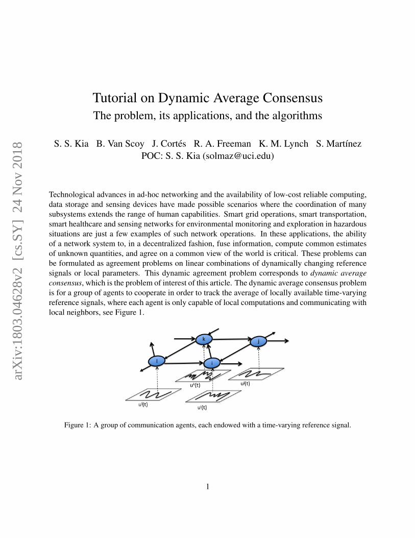
Technological advances in ad-hoc networking and the availability of low-cost reliable computing,data storage and sensing devices have made possible scenarios where the coordination of manysubsystems extends the range of human capabilities. Smart grid operations, smart transportation,smart healthcare and sensing networks for environmental monitoring and exploration in hazardoussituations are just a few examples of such network operations. In these applications, the abilityof a network system to, in a decentralized fashion, fuse information, compute common estimatesof unknown quantities, and agree on a common view of the world is critical. These problems canbe formulated as agreement problems on linear combinations of dynamically changing referencesignals or local parameters. This dynamic agreement problem corresponds to dynamic averageconsensus, which is the problem of interest of this article. The dynamic average consensus problemis for a group of agents to cooperate in order to track the average of locally available time-varyingreference signals, where each agent is only capable of local computations and communicating withlocal neighbors, see Figure 1.

Figure 1: A group of communication agents, each endowed with a time-varying reference signal.

1

arX

iv:1

803.

0462

8v2

[cs

.SY

] 2

4 N

ov 2

018

Centralized solutions have drawbacks

The difficulty in the dynamic average consensus problem is that the information is distributedacross the network. A straightforward solution, termed centralized, to the dynamic average con-sensus problem appears to be to gather all of the information in a single place, do the computation(in other words, calculate the average), and then send the solution back through the network to eachagent. Although simple, the centralized approach has numerous drawbacks: (1) the algorithm isnot robust to failures of the centralized agent (if the centralized agent fails, then the entire computa-tion fails), (2) the method is not scalable since the amount of communication and memory requiredon each agent scales with the size of the network, (3) each agent must have a unique identifier (sothat the centralized agent counts each value only once), (4) the calculated average is delayed by anamount which grows with the size of the network, and (5) the reference signals from each agentare exposed over the entire network which is unacceptable in applications involving sensitive data.The centralized solution is fragile due to existence of a single failure point in the network. Thiscan be overcome by having every agent act as the centralized agent. In this approach, referred toas flooding, agents transmit the values of the reference signals across the entire network until eachagent knows each reference signal. This may be summarized as “first do all communications, thendo all computations”. While flooding fixes the issue of robustness to agent failures, it is still subjectto many of the drawbacks of the centralized solution. Also, although this approach works reason-ably well for small size networks, its communication and storage costs scale poorly in terms ofthe network size and may incur, depending on how it is implemented, in costs of order O(N2) peragent (for instance, if each agent has to maintain, for each piece of information, which neighbor ithas sent it to and which it has not. This motivates the interest in developing distributed solutions forthe dynamics average consensus problem that only involve local interactions and decisions amongthe agents.

Multiple instantiations of static average consensus algorithms are not able to deal with dy-namic problems

It is likely that the reader is familiar with the static version of the dynamic average consensusproblem, commonly referred to as static average consensus, where agents seek to agree on a spe-cific combination of fixed quantities. The static problem has been extensively studied in the litera-ture [1, 2, 3, 4], and several simple and efficient distributed algorithms exist with exact convergenceguarantees. Given its mature literature, a natural approach to deal with the distributed solution ofthe dynamic average consensus problem in some literature has been to zero-order sample the ref-erence signals and use a static average consensus algorithm between sampling times (for example,see [5, 6]). If this approach were practical, it would mean that there is no need to worry aboutdesigning specific algorithms to solve the dynamic average consensus problem, since we couldrely on the algorithmic solutions available for static average consensus.

As the reader might have correctly guessed already, this approach does not work. In order for it

2

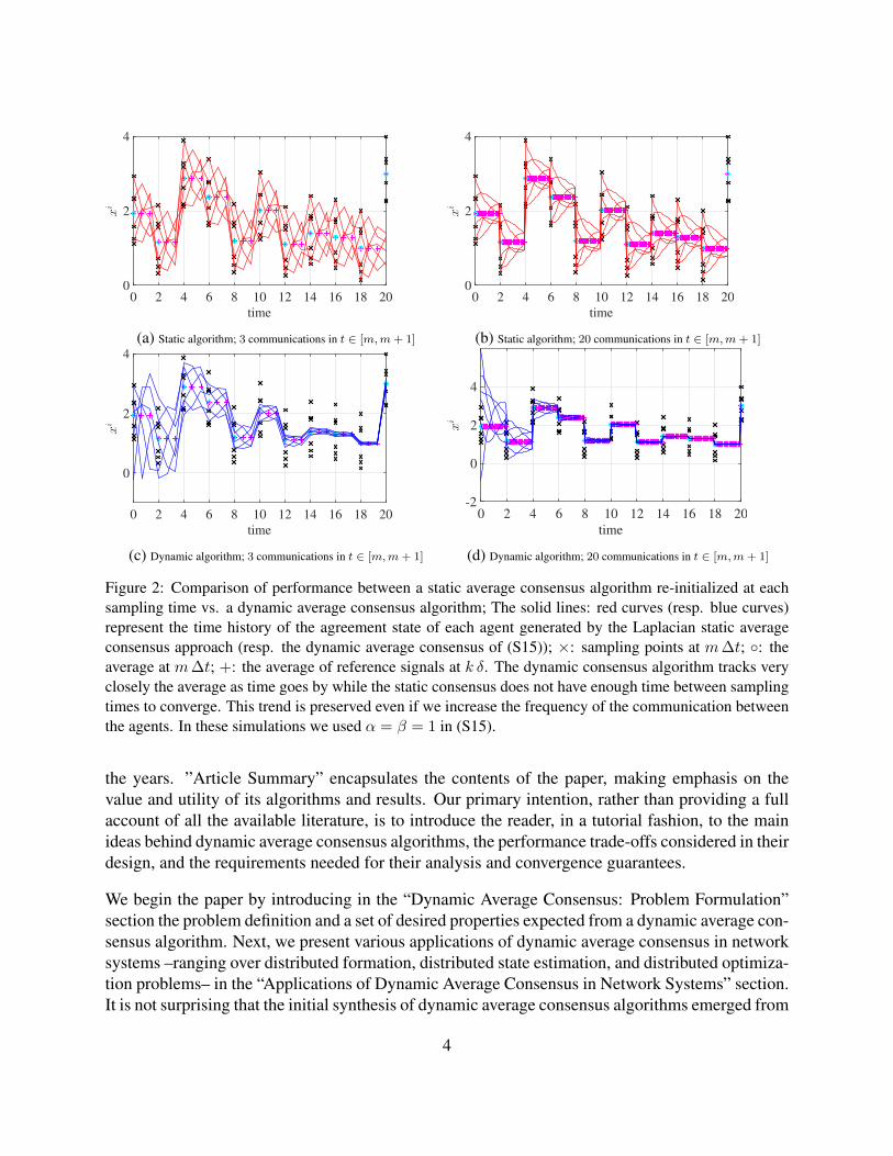
to work, we would essentially need a static average consensus algorithm which is able to converge‘infinitely’ fast. In practice, some time is required for information to flow across the network,and hence the result of the repeated application of any static average consensus algorithm operateswith some error whose size depends on its speed of convergence and how fast inputs change. Toillustrate this point better, consider the following numerical example. Consider a process describedby a fixed value plus a sine wave whose frequency and phase are changing randomly over time.A group of 6 agents with the communication topology of directed ring monitors this process bytaking synchronous samples, each according to

ui(m) = ai (2 + sin(ω(m)t(m) + φ(m))) + bi, m ∈ Z≥0,

where ai and bi are fixed unknown error sources in the measurement of agent i ∈ {1, . . . , 6}.To reduce the effect of measurement errors, after each sampling, every agent wants to obtain theaverage of the measurements across the network before the next sampling time. For the numericalsimulations, the values ω ∼ N(0, 0.25), φ ∼ N(0, (π/2)2), with N(µ, p) indicating a Gaussiandistribution with mean µ and variance p are used. We set the sampling rate at 0.5 hz (∆t = 2 s).For the simulation under study we use a1 = 1.1, a2 = 1, a3 = 0.9, a4 = 1.05, a5 = 0.96, a6 = 1,b1 = −0.55, b2 = 1, b3 = 0.6, b4 = −0.9, b5 = −0.6, and b6 = 0.4. To obtain the average, weuse the following two approaches: (a) at every sampling timem, each agent initializes the standardstatic discrete-time Laplacian average consensus algorithm

xi(k + 1) = xi(k)− δN∑j=1

aij(xi(k)− xj(k)), i ∈ {1, . . . , N},

by the current sampled reference values, xi(0) = ui(m), and implements it with an admissibletimestep δ until just before the next sampling time m+ 1; (b) at time m = 0, agents start executinga dynamic average consensus algorithm (more specifically, the strategy (S15) which is described indetail later). Between sampling times m and m + 1, the reference input ui(k) implemented in thealgorithm is fixed at ui(m), where here k is the communication time index. Figure 2 compares thetracking performance of these two approaches. We can observe that the dynamic average consensusalgorithm, by keeping a memory of past actions, produces a better tracking response than the staticalgorithm initialized at each sampling time with the current values. This comparison serves asmotivation for the need of specifically designed distributed algorithms that take into account theparticular features of the dynamic average consensus problem.

Objectives and roadmap of the article

The objective of this article is to provide an overview of the dynamic average consensus problemthat serves as a comprehensive introduction to the problem definition, its applications, and thedistributed methods available to solve them. We decided to write this article after realizing thatthere exist in the literature many works that have dealt with the problem, but that there does notexist a tutorial reference that presents in a unified way the developments that have occurred over

3

time

0 2 4 6 8 10 12 14 16 18 20

xi

0

2

4

(a) Static algorithm; 3 communications in t ∈ [m,m+ 1]

time

0 2 4 6 8 10 12 14 16 18 20

xi

0

2

4

(b) Static algorithm; 20 communications in t ∈ [m,m+ 1]

time

0 2 4 6 8 10 12 14 16 18 20

xi

0

2

4

(c) Dynamic algorithm; 3 communications in t ∈ [m,m+ 1]

time

0 2 4 6 8 10 12 14 16 18 20

xi

-2

0

2

4

(d) Dynamic algorithm; 20 communications in t ∈ [m,m+ 1]

Figure 2: Comparison of performance between a static average consensus algorithm re-initialized at eachsampling time vs. a dynamic average consensus algorithm; The solid lines: red curves (resp. blue curves)represent the time history of the agreement state of each agent generated by the Laplacian static averageconsensus approach (resp. the dynamic average consensus of (S15)); ×: sampling points at m∆t; ◦: theaverage at m∆t; +: the average of reference signals at k δ. The dynamic consensus algorithm tracks veryclosely the average as time goes by while the static consensus does not have enough time between samplingtimes to converge. This trend is preserved even if we increase the frequency of the communication betweenthe agents. In these simulations we used α = β = 1 in (S15).

the years. ”Article Summary” encapsulates the contents of the paper, making emphasis on thevalue and utility of its algorithms and results. Our primary intention, rather than providing a fullaccount of all the available literature, is to introduce the reader, in a tutorial fashion, to the mainideas behind dynamic average consensus algorithms, the performance trade-offs considered in theirdesign, and the requirements needed for their analysis and convergence guarantees.

We begin the paper by introducing in the “Dynamic Average Consensus: Problem Formulation”section the problem definition and a set of desired properties expected from a dynamic average con-sensus algorithm. Next, we present various applications of dynamic average consensus in networksystems –ranging over distributed formation, distributed state estimation, and distributed optimiza-tion problems– in the “Applications of Dynamic Average Consensus in Network Systems” section.It is not surprising that the initial synthesis of dynamic average consensus algorithms emerged from

4

a careful look at static average consensus algorithms. In the “A Look at Static Average ConsensusLeading up to the Design of a Dynamic Average Consensus Algorithm” section, we provide a briefreview of standard algorithms for the static average consensus, and then build on this discussion todescribe the first dynamic average consensus algorithm presented in the paper. We also elaborateon various features of these initial algorithms and identify their shortcomings. This sets the stageto introduce in the “Continuous-Time Dynamic Average Consensus Algorithms” section variousalgorithms that aim to address these shortcomings. The design of continuous-time algorithms fornetwork systems is often motivated by the conceptual ease for design and analysis, rooted in therelatively mature theoretical basis for the control of continuous-time systems. However, the imple-mentation of these continuous-time algorithms on cyber-physical systems may not be feasible dueto practical constraints such as limited inter-agent communication bandwidth. This motivates the“Discrete-Time Dynamic Average Consensus Algorithms” section, where we specifically discussmethods to accelerate the convergence rate and enhance the robustness of the proposed algorithms.Since the information of each agent takes some time to propagate through the network, we canexpect that tracking an arbitrarily fast average signal with zero error is not feasible unless agentshave some a priori information about the dynamics generating the signals. We address this topicin the “Perfect Tracking Using A Priori Knowledge of the Input Signals” section, where we takeadvantage of knowledge of the nature of the reference signals. Many other topics exist that arerelated to the dynamic average consensus problem that we do not explore in this article. Interestedreader can find several intriguing pointers for such topics in “Further Reading”. Throughout thepaper, unless otherwise noted, we consider network systems whose communication topology isdescribed by strongly connected and weight-balanced directed graphs. Only in a couple of spe-cific cases, we particularize our discussion to the setup of undirected graphs, and we make explicitmention of this to the reader.

Required mathematical background and available resources for implementation

Graph theory plays an essential role in design and performance analysis of dynamic consensusalgorithms. “Basic Notations from Graph Theory” provides a brief overview of the relevant graphtheoretic concepts, definitions and notations that we use in the article. Dynamic average consensusalgorithms are linear time-invariant (LTI) systems in which the reference signals of the agentsenter the system as an external input, in contrast to (Laplacian) static average consensus algorithmwhere the reference signals enter as initial conditions. Thus, in addition to the internal stabilityanalysis, which is sufficient for the static average consensus algorithm, we need to asses the input-to-state stability (ISS) of the algorithms. The reader can find a brief overview of the ISS analysisof LTI systems in “Input-to-State Stability of LTI Systems”. All of the algorithms described canbe implemented using modern computing languages such as C and Matlab. Furthermore, Matlabprovides functions for simple construction, modification, and visualization of graphs.

5

Dynamic Average Consensus: Problem Formulation

Consider a group ofN agents where each agent is capable of (1) sending and receiving informationwith other agents, (2) storing information, and (3) performing local computations. For example,the agents may be cooperating robots or sensors in a wireless sensor network. The communicationtopology among the agents is described by a fixed digraph, see “Basic Notations from GraphTheory” for further details and the graph related notations used throughout the article. Supposethat each agent has a local scalar reference signal, denoted ui(t) : [0,∞) → R in continuous timeand ui(k) : N→ R in discrete time. This signal may be the output of a sensor located on the agent,or it could be the output of another algorithm that the agent is running. The dynamic averageconsensus problem then consists of designing an algorithm that allows individual agents to trackthe time-varying average of the reference signals, given by

CT: uavg(t) :=1

N

∑N

i=1ui(t)

DT: uavg(k) :=1

N

∑N

i=1ui(k)

in continuous time (CT) and discrete time (DT), respectively. For discrete-time signals and algo-rithms, for any variable p sampled at time tk, we use the shorthand notation p(k) or pk to referto p(tk). For reasons that we specify below, we are specifically interested in the design of dis-tributed algorithms, meaning that to obtain the average, the policy that each agent implements onlydepends on its variables (represented by J i, which include its own reference signal) and those ofits out-neighbors (represented by {Ij}j∈N iout

).

In continuous time, we seek a driving command ci(J i(t), {Ij(t)}j∈N iout) ∈ R for each agent i ∈

{1, . . . , N} such that, with perhaps an appropriate initialization, a local state xi(t), which we referto as the agreement state of agent i, converges to the average uavg(t) asymptotically. Formally, for

CT : xi = ci(J i(t), {Ij(t)}j∈N iout), i ∈ {1, . . . , N}, (1)

with proper initialization if necessary, we have xi(t)→ uavg(t) as t→∞. The driving command ci

can be a memoryless function or an output of a local internal dynamics. Note that, by using the out-neighbors, we are making the convention that information flows in the opposite direction specifiedby a directed edge (there is no loss of generality in doing it so, and the alternative convention ofusing in-neighbors instead would also be equally valid).

Dynamic average consensus can also be accomplished using discrete-time dynamics, especiallywhen the time-varying inputs are sampled at discrete times. In such a case, we seek a drivingcommand for each agent i ∈ {1, . . . , N} so that

DT : xi(tk+1) = ci(J i(tk), {Ij(tk)}j∈N iout), i ∈ {1, . . . , N}, (2)

under proper initialization if necessary, accomplishes xi(tk)→ uavg(k) as tk →∞. Algorithm 1 il-lustrates how a discrete-time dynamic average consensus algorithm can be executed over a networkof N communicating agents.

6

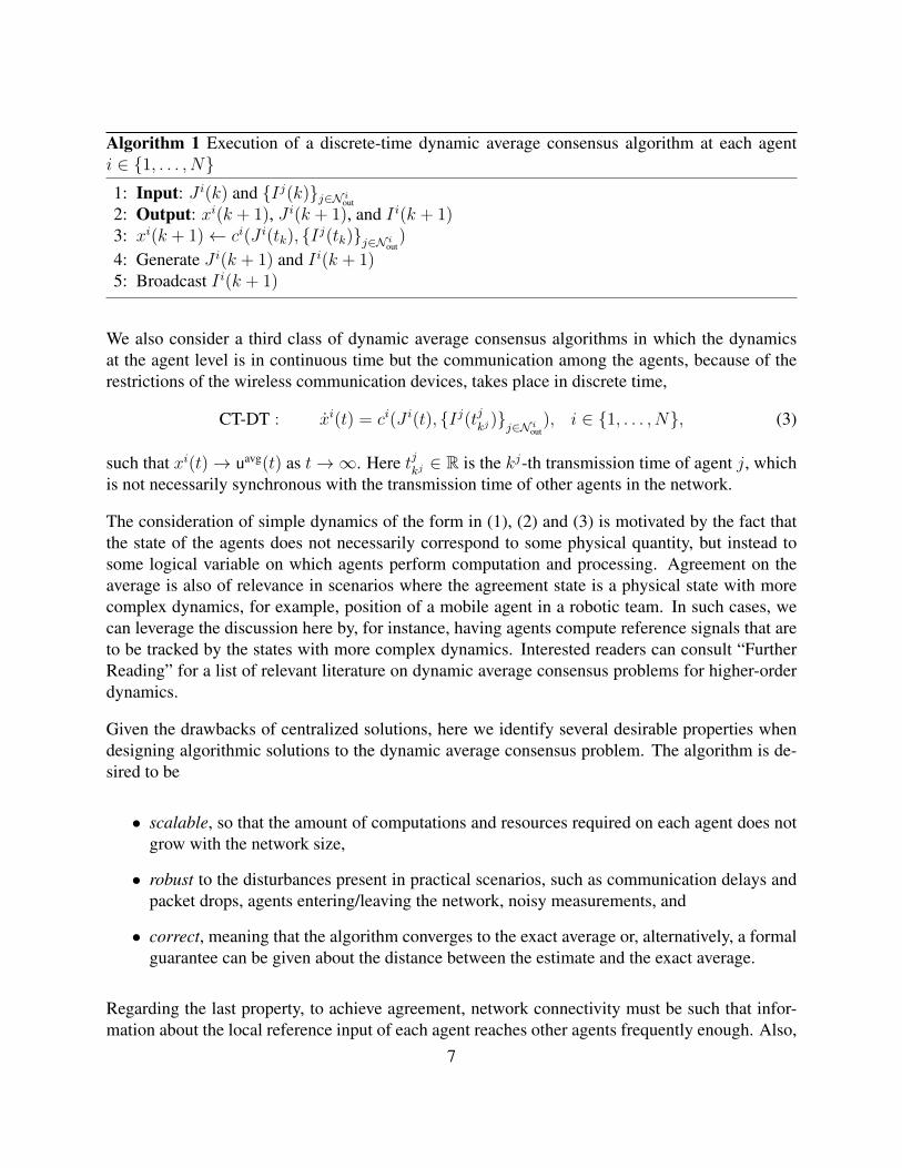
Algorithm 1 Execution of a discrete-time dynamic average consensus algorithm at each agenti ∈ {1, . . . , N}1: Input: J i(k) and {Ij(k)}j∈N iout

2: Output: xi(k + 1), J i(k + 1), and I i(k + 1)3: xi(k + 1)← ci(J i(tk), {Ij(tk)}j∈N iout

)

4: Generate J i(k + 1) and I i(k + 1)5: Broadcast I i(k + 1)

We also consider a third class of dynamic average consensus algorithms in which the dynamicsat the agent level is in continuous time but the communication among the agents, because of therestrictions of the wireless communication devices, takes place in discrete time,

CT-DT : xi(t) = ci(J i(t), {Ij(tjkj

)}j∈N iout

), i ∈ {1, . . . , N}, (3)

such that xi(t)→ uavg(t) as t→∞. Here tjkj∈ R is the kj-th transmission time of agent j, which

is not necessarily synchronous with the transmission time of other agents in the network.

The consideration of simple dynamics of the form in (1), (2) and (3) is motivated by the fact thatthe state of the agents does not necessarily correspond to some physical quantity, but instead tosome logical variable on which agents perform computation and processing. Agreement on theaverage is also of relevance in scenarios where the agreement state is a physical state with morecomplex dynamics, for example, position of a mobile agent in a robotic team. In such cases, wecan leverage the discussion here by, for instance, having agents compute reference signals that areto be tracked by the states with more complex dynamics. Interested readers can consult “FurtherReading” for a list of relevant literature on dynamic average consensus problems for higher-orderdynamics.

Given the drawbacks of centralized solutions, here we identify several desirable properties whendesigning algorithmic solutions to the dynamic average consensus problem. The algorithm is de-sired to be

• scalable, so that the amount of computations and resources required on each agent does notgrow with the network size,

• robust to the disturbances present in practical scenarios, such as communication delays andpacket drops, agents entering/leaving the network, noisy measurements, and

• correct, meaning that the algorithm converges to the exact average or, alternatively, a formalguarantee can be given about the distance between the estimate and the exact average.

Regarding the last property, to achieve agreement, network connectivity must be such that infor-mation about the local reference input of each agent reaches other agents frequently enough. Also,

7

as the information of each agent takes some time to propagate through the network, tracking anarbitrarily fast average signal with zero error is not feasible unless agents have some a priori in-formation about the dynamics generating the signals. Therefore, a recurring theme throughout thearticle is how the convergence guarantees of dynamic average consensus algorithms depend on thenetwork connectivity and on the rate of change of the reference signal of each agent.

Applications of Dynamic Average Consensus in Network Systems

The ability to compute the average of a set of time-varying reference signals turns out to be usefulin numerous applications, and this explains why distributed algorithmic solutions have found theirway into many seemingly different problems involving the interconnection of dynamical systems.This section provides a selected overview of problems to further motivate the reader to learn aboutdynamic average consensus algorithms and illustrate their range of applicability. Other applica-tions of dynamic average consensus can be found in [7, 8, 9, 10, 11, 12, 13].

Distributed formation control

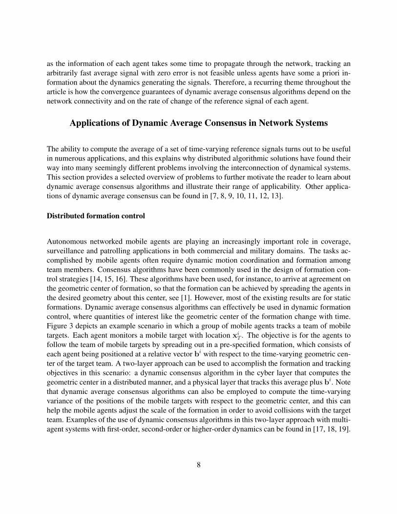
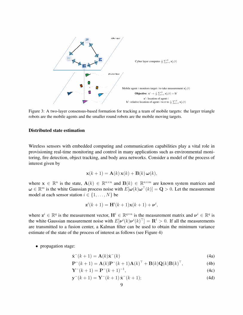
Autonomous networked mobile agents are playing an increasingly important role in coverage,surveillance and patrolling applications in both commercial and military domains. The tasks ac-complished by mobile agents often require dynamic motion coordination and formation amongteam members. Consensus algorithms have been commonly used in the design of formation con-trol strategies [14, 15, 16]. These algorithms have been used, for instance, to arrive at agreement onthe geometric center of formation, so that the formation can be achieved by spreading the agents inthe desired geometry about this center, see [1]. However, most of the existing results are for staticformations. Dynamic average consensus algorithms can effectively be used in dynamic formationcontrol, where quantities of interest like the geometric center of the formation change with time.Figure 3 depicts an example scenario in which a group of mobile agents tracks a team of mobiletargets. Each agent monitors a mobile target with location xiT . The objective is for the agents tofollow the team of mobile targets by spreading out in a pre-specified formation, which consists ofeach agent being positioned at a relative vector bi with respect to the time-varying geometric cen-ter of the target team. A two-layer approach can be used to accomplish the formation and trackingobjectives in this scenario: a dynamic consensus algorithm in the cyber layer that computes thegeometric center in a distributed manner, and a physical layer that tracks this average plus bi. Notethat dynamic average consensus algorithms can also be employed to compute the time-varyingvariance of the positions of the mobile targets with respect to the geometric center, and this canhelp the mobile agents adjust the scale of the formation in order to avoid collisions with the targetteam. Examples of the use of dynamic consensus algorithms in this two-layer approach with multi-agent systems with first-order, second-order or higher-order dynamics can be found in [17, 18, 19].

8

xi: location of agent ibi: relative location of agent i w.r.t to 1

N

∑Ni=1 xiT (t)

Mobile agent i monitors target i to take measurement xiT (t)

Objective: xi → 1N

∑Ni=1 xiT (t) + bi

Cyber layer computes 1N

∑Ni=1 xiT (t)

Figure 3: A two-layer consensus-based formation for tracking a team of mobile targets: the larger trianglerobots are the mobile agents and the smaller round robots are the mobile moving targets.

Distributed state estimation

Wireless sensors with embedded computing and communication capabilities play a vital role inprovisioning real-time monitoring and control in many applications such as environmental moni-toring, fire detection, object tracking, and body area networks. Consider a model of the process ofinterest given by

x(k + 1) = A(k) x(k) + B(k)ω(k),

where x ∈ Rn is the state, A(k) ∈ Rn×n and B(k) ∈ Rn×m are known system matrices andω ∈ Rm is the white Gaussian process noise with E[ω(k)ω>(k)] = Q > 0. Let the measurementmodel at each sensor station i ∈ {1, . . . , N} be

zi(k + 1) = Hi(k + 1)x(k + 1) + νi,

where zi ∈ Rq is the measurement vector, Hi ∈ Rq×n is the measurement matrix and νi ∈ Rq isthe white Gaussian measurement noise with E[νi(k)νi(k)>] = Ri > 0. If all the measurementsare transmitted to a fusion center, a Kalman filter can be used to obtain the minimum varianceestimate of the state of the process of interest as follows (see Figure 4)

• propagation stage:

x−(k + 1) = A(k)x−(k) (4a)

P−(k + 1) = A(k)P−(k + 1)A(k)> + B(k)Q(k)B(k)>, (4b)Y−(k + 1) = P−(k + 1)−1, (4c)

y−(k + 1) = Y−(k + 1) x−(k + 1); (4d)9

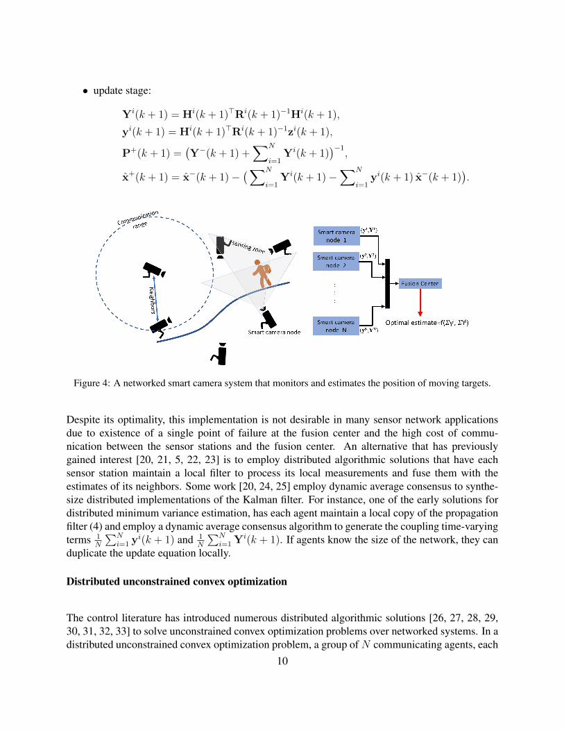
• update stage:

Yi(k + 1) = Hi(k + 1)>Ri(k + 1)−1Hi(k + 1),

yi(k + 1) = Hi(k + 1)>Ri(k + 1)−1zi(k + 1),

P+(k + 1) =(Y−(k + 1) +

∑N

i=1Yi(k + 1)

)−1,

x+(k + 1) = x−(k + 1)−(∑N

i=1Yi(k + 1)−

∑N

i=1yi(k + 1) x−(k + 1)

).

Figure 4: A networked smart camera system that monitors and estimates the position of moving targets.

Despite its optimality, this implementation is not desirable in many sensor network applicationsdue to existence of a single point of failure at the fusion center and the high cost of commu-nication between the sensor stations and the fusion center. An alternative that has previouslygained interest [20, 21, 5, 22, 23] is to employ distributed algorithmic solutions that have eachsensor station maintain a local filter to process its local measurements and fuse them with theestimates of its neighbors. Some work [20, 24, 25] employ dynamic average consensus to synthe-size distributed implementations of the Kalman filter. For instance, one of the early solutions fordistributed minimum variance estimation, has each agent maintain a local copy of the propagationfilter (4) and employ a dynamic average consensus algorithm to generate the coupling time-varyingterms 1

N

∑Ni=1 yi(k + 1) and 1

N

∑Ni=1 Yi(k + 1). If agents know the size of the network, they can

duplicate the update equation locally.

Distributed unconstrained convex optimization

The control literature has introduced numerous distributed algorithmic solutions [26, 27, 28, 29,30, 31, 32, 33] to solve unconstrained convex optimization problems over networked systems. In adistributed unconstrained convex optimization problem, a group of N communicating agents, each

10

with access to a local convex cost function f i : Rn → R, i ∈ {1, . . . , N}, seek to determine theminimizer of the joint global optimization problem

x? = argmin1

N

∑N

i=1f i(x), (5)

by local interactions with their neighboring agents. This problem appears in network system ap-plications such as multi-agent coordination, distributed state estimation over sensor networks, orlarge scale machine learning problems. Some of the algorithmic solutions for this problem aredeveloped using agreement algorithms to compute global quantities that appear in existing cen-tralized algorithms. For example, a centralized solution for (5) is the Nesterov gradient descentalgorithm [34] described by

x(k + 1) = y(k)− η (1

N

∑N

i=1∇f i(y(k))), (6a)

v(k + 1) = y(k)− η

αk(

1

N

∑N

i=1∇f i(y(k))), (6b)

y(k + 1) = (1− αk+1) x(k + 1) + αt+1v(k + 1). (6c)

where x(0),y(0),v(0) ∈ Rn, and {αk}∞k=0 is defined by an arbitrarily chosen α0 ∈ (0, 1) and theupdate equation α2

k+1 = (1−αk+1)α2k, where αk+1 always takes the unique solution in (0, 1). If all

f i, i ∈ {1, . . . , N}, are convex, differentiable and have L-Lipschitz gradients, then every trajectoryk 7→x(k) of (6) converges to the optimal solution x? for any 0 < η < 1

L.

Note that in (6), the cumulative gradient term 1N

∑Ni=1∇f i(y(k)) is a source of coupling among

the computations performed by each agent. It does not seem reasonable to halt the execution ofthis algorithm at each step until the agents have figured out the value of this term. Instead, wecould employ dynamic average consensus in conjunction with (6): the dynamic average consensusalgorithm estimates the coupling term, this estimate is employed in executing (6), which in turnchanges the value of the coupling term being estimated. This approach is taken in [33] to solvethe optimization problem (5) over connected graphs, and also pursued in other implementations ofdistributed convex or nonconvex optimization algorithms, see for instance [35, 36, 37, 38, 39].

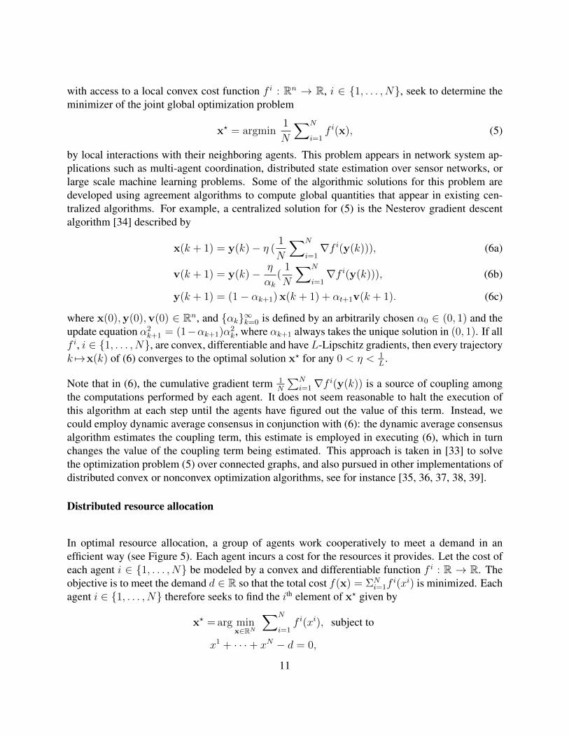
Distributed resource allocation

In optimal resource allocation, a group of agents work cooperatively to meet a demand in anefficient way (see Figure 5). Each agent incurs a cost for the resources it provides. Let the cost ofeach agent i ∈ {1, . . . , N} be modeled by a convex and differentiable function f i : R → R. Theobjective is to meet the demand d ∈ R so that the total cost f(x) = ΣN

i=1fi(xi) is minimized. Each

agent i ∈ {1, . . . , N} therefore seeks to find the ith element of x? given by

x? = arg minx∈RN

∑N

i=1f i(xi), subject to

x1 + · · ·+ xN − d = 0,

11

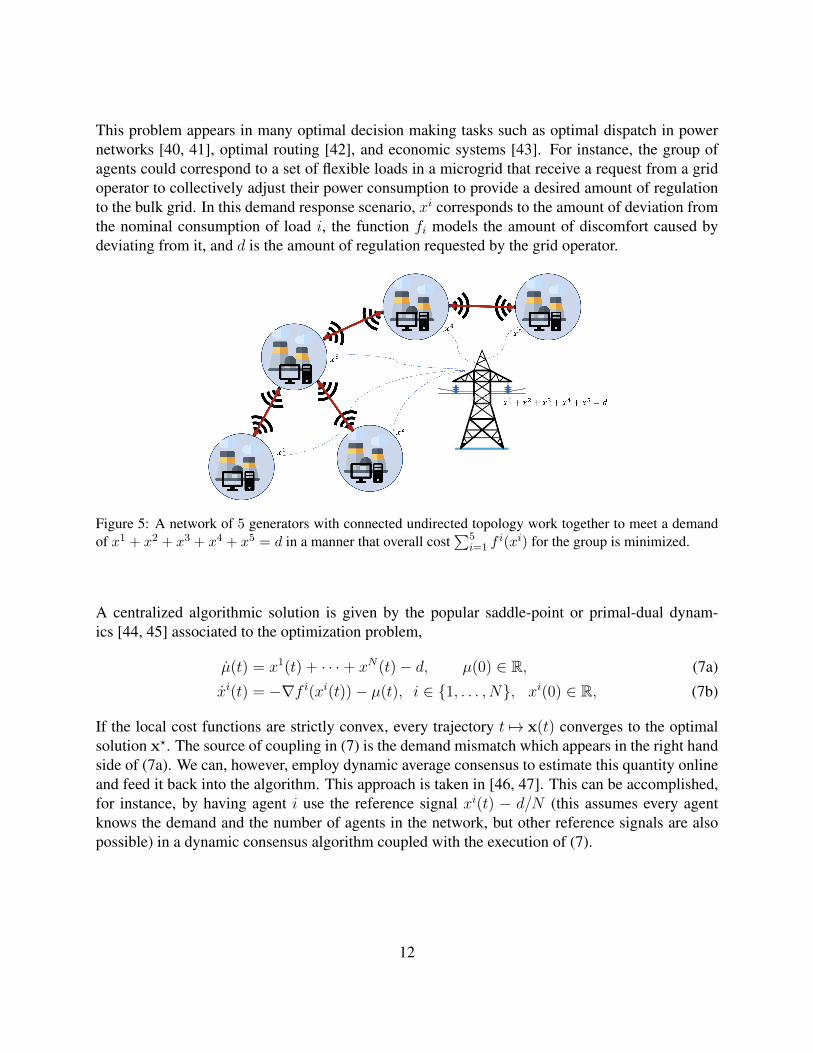
This problem appears in many optimal decision making tasks such as optimal dispatch in powernetworks [40, 41], optimal routing [42], and economic systems [43]. For instance, the group ofagents could correspond to a set of flexible loads in a microgrid that receive a request from a gridoperator to collectively adjust their power consumption to provide a desired amount of regulationto the bulk grid. In this demand response scenario, xi corresponds to the amount of deviation fromthe nominal consumption of load i, the function fi models the amount of discomfort caused bydeviating from it, and d is the amount of regulation requested by the grid operator.

Figure 5: A network of 5 generators with connected undirected topology work together to meet a demandof x1 + x2 + x3 + x4 + x5 = d in a manner that overall cost

∑5i=1 f

i(xi) for the group is minimized.

A centralized algorithmic solution is given by the popular saddle-point or primal-dual dynam-ics [44, 45] associated to the optimization problem,

µ(t) = x1(t) + · · ·+ xN(t)− d, µ(0) ∈ R, (7a)

xi(t) = −∇f i(xi(t))− µ(t), i ∈ {1, . . . , N}, xi(0) ∈ R, (7b)

If the local cost functions are strictly convex, every trajectory t 7→ x(t) converges to the optimalsolution x?. The source of coupling in (7) is the demand mismatch which appears in the right handside of (7a). We can, however, employ dynamic average consensus to estimate this quantity onlineand feed it back into the algorithm. This approach is taken in [46, 47]. This can be accomplished,for instance, by having agent i use the reference signal xi(t) − d/N (this assumes every agentknows the demand and the number of agents in the network, but other reference signals are alsopossible) in a dynamic consensus algorithm coupled with the execution of (7).

12

A Look at Static Average Consensus Leading up to the Design of a DynamicAverage Consensus Algorithm

Consensus algorithms to solve the static average consensus problem have been studied at least asfar back as [48]. The commonality in their design is the idea of having agents start their agreementstate with their own reference value and adjust it based on some weighted linear feedback whichtakes into account the difference between their agreement state and their neighbors’. This leads toalgorithms of the following form

CT: xi(t) = −N∑j=1

aij(xi(t)− xj(t)

), (8a)

DT: xi(k + 1) = xi(k)−N∑j=1

aij(xi(k)− xj(k)

), (8b)

for i ∈ {1, . . . , N}, with xi(0) = ui constant for both algorithms. Here [aij]N×N is the adjacencymatrix of the communication graph (see “Basic Notions from Graph Theory”). By stacking theagent variables into vectors, the static average consensus algorithms can be written compactlyusing a graph Laplacian as

CT: x(t) = −Lx(t), (9a)DT: x(k + 1) = (I− L) x(k), (9b)

with x(0) = u. When the communication graph is fixed, this system is linear time invariant and canbe analyzed using standard time domain and frequency-domain techniques in control. Specifically,the frequency-domain representation of the dynamic average consensus algorithm output signal isgiven by

CT: X(s) = [sI + L]−1x(0) = [sI + L]−1U(s) (10a)DT: X(z) = [zI− (I− L)]−1U(z), (10b)

where X(s) and U(s), respectively, denote the Laplace transform of x(t) and u, while X(z) andU(z), respectively, denote the z-transform of Xk and u. For a static signals we have U(s) = u andU(z) = u.

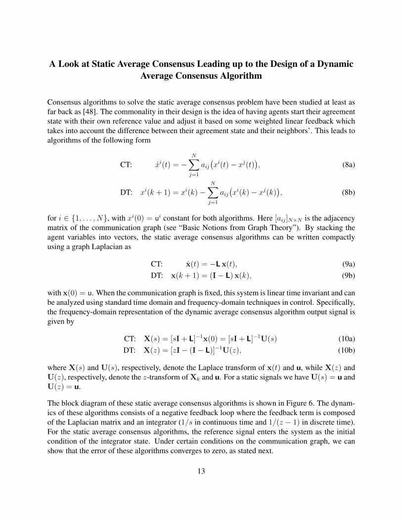
The block diagram of these static average consensus algorithms is shown in Figure 6. The dynam-ics of these algorithms consists of a negative feedback loop where the feedback term is composedof the Laplacian matrix and an integrator (1/s in continuous time and 1/(z − 1) in discrete time).For the static average consensus algorithms, the reference signal enters the system as the initialcondition of the integrator state. Under certain conditions on the communication graph, we canshow that the error of these algorithms converges to zero, as stated next.

13

1

sIN

L

x(t)

x(0)−

(a) Continuous time

1

z − 1IN

L

xk

x0

−

(b) Discrete time

Figure 6: Block diagram of the static average consensus algorithms (9). The input signals are assigned tothe initial conditions, that is, x(0) = u (in continuous time) or x0 = u (in discrete time). The feedback loopconsists of the Laplacian matrix of the communication graph and an integrator (1/s in continuous time and1/(z − 1) in discrete time).

Theorem 1 (Convergence guarantees of the CT and DT static average consensus al-gorithms (8) [1]). Suppose that the communication graph is constant, strongly connected, andweight-balanced digraph, and that the reference signal ui at each agent i ∈ {1, . . . , N} is aconstant scalar. Then the following convergence results hold for the CT and DT static averageconsensus algorithms (8)

CT: As t → ∞ every agreement state xi(t), i ∈ {1, . . . , N} of the CT static average consensusalgorithm (8a) converges to uavg with an exponential rate no worse than λ2, the smallestnonzero eigenvalue of Sym(L).

DT: As k → ∞ every agreement state xik, i ∈ {1, . . . , N} of the DT static average consensusalgorithm (8b) converges to uavg with an exponential rate no worse than ρ ∈ (0, 1), providedthat the Laplacian matrix satisfies ρ = ‖IN − L− 1N1>N/N‖2 < 1.

Note that, given a weighted graph with Laplacian matrix L, we can scale the graph weights by anonzero constant δ ∈ R to produce a scaled Laplacian matrix δL, see “Basic Notions from GraphTheory.” This extra scaling parameter can then be used to produce a Laplacian matrix that satisfiesthe conditions in Theorem 1.

A first design for dynamic average consensus

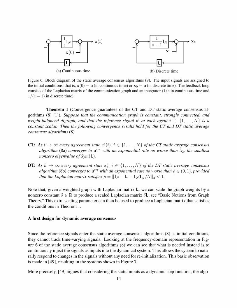
Since the reference signals enter the static average consensus algorithms (8) as initial conditions,they cannot track time-varying signals. Looking at the frequency-domain representation in Fig-ure 6 of the static average consensus algorithms (8) we can see that what is needed instead is tocontinuously inject the signals as inputs into the dynamical system. This allows the system to natu-rally respond to changes in the signals without any need for re-initialization. This basic observationis made in [49], resulting in the systems shown in Figure 7.

More precisely, [49] argues that considering the static inputs as a dynamic step function, the algo-14

u(t)1

sIN

L

x(t)

x(0)−

(a) Dynamic average consensus algorithm (11)

u(t)

1

sIN L

x(t)

p(0)

−

(b) Dynamic average consensus algorithm (16)

Figure 7: Block diagram of the continuous-time dynamic average consensus algorithms (11) and (16).While the reference signals are applied as initial conditions for the static consensus algorithms, the referencesignals are here applied as inputs to the system. Although both systems are equivalent, system (a) is in theform (3) and explicitly requires the derivative of the reference signals, while system (b) does not requiredifferentiating the reference signals.

rithm

x(t) = −Lx(t) + u(t), xi(0) = ui(0), ui(t) = uih(t), i ∈ {1, . . . , N},

in which the reference value of the agents enter the dynamics as an external input, results in thesame frequency representation (10a) (here h(t) is the Heaviside step function). Therefore, conver-gence to the average of reference values is guaranteed. Based on this observation, [49] proposesone of the earliest algorithms for dynamic average consensus,

xi(t) = −N∑j=1

aij(xi(t)− xj(t)) + ui(t), i ∈ {1, . . . , N}, (11a)

xi(0) = ui(0). (11b)

Using a Laplace domain analysis, [49] shows that, if each input signal ui, i ∈ {1, . . . , N}, hasa Laplace transform with all poles in the left half-plane and at most one zero pole (such signalsare asymptotically constant), all the agents implementing algorithm (11) over a connected graphtrack uavg(t) with zero error asymptotically. As we show below, the convergence properties ofalgorithm (11) can be described more comprehensively using time-domain ISS analysis.

Define the tracking error of agent i by

ei(t) = xi(t)− uavg(t), i ∈ {1, . . . , N}.

To analyze the system, the error is decomposed into the consensus direction (that is, the direction1N ) and the disagreement directions (that is, the directions orthogonal to 1N ). To this end, definethe transformation matrix T =

[1√N

1N R]

where R ∈ RN×(N−1) is such that T>T = TT> =

IN , and consider the change of variables

e =

[e1

e2:N

]= T>e. (12)

15

In the new coordinates, (11) takes the form

˙e1 = 0, e1(t0) =1√N

∑N

j=1(xi(t0)− ui(t0)), (13a)

˙e2:N = −R> LR e2:N + R>u, e2:N(t0) = R> x(t0), (13b)

where t0 is the initial time. Using the ISS bound on the trajectories of LTI systems (see “Input-to-State Stability of LTI Systems”), the tracking error of each agent i ∈ {1, . . . , N} while im-plementing (11) over a strongly connected and weight-balanced digraph is (here we use Π =(IN − 1

N1N1>N))

|ei(t)| ≤√‖e2:N(t)‖2 + |e1(t)|2

≤

√(e−λ2 (t−t0)‖Πx(t0)‖+

supt0≤τ≤t ‖Πu(τ)‖λ2

)2

+(∑N

j=1(xi(t0)− ui(t0))√N

)2

, (14)

for all t ∈ [t0,∞), where λ2 is the smallest nonzero eigenvalue of Sym(L).

The tracking error bound (14) reveals several interesting facts. First, it highlights the necessity forthe special initialization (11b). Without it, a fixed offset from perfect tracking is present regardlessof the type of reference input signals –instead, we would expect that a proper dynamic consensusalgorithm should be capable of perfectly tracking static reference signals. Next, (14) shows that thealgorithm (11) renders perfect asymptotic tracking not only for reference input signals with decay-ing rate, but also for unbounded reference signals whose uncommon parts asymptotically convergeto a constant value. This fact is due to the ISS tracking bound depending on ‖(IN− 1

N1N1>N)u(τ)‖

rather than on ‖u(τ)‖. Note that if the reference signal of each agent i ∈ {1, . . . , N} can be writ-ten as ui(t) = u(t) + ui(t), where u(t) is the (possibly unbounded) common part and ui(t) is theuncommon part of the reference signal, we obtain

‖(IN −1

N1N1>N)u(τ)‖ = ‖(IN −

1

N1N1>N)(u(t)1N + ˙u(t))‖ = ‖(IN −

1

N1N1>N) ˙u(t)‖.

This goes to show that the algorithm (11) properly uses the local knowledge about the unboundedbut common part of the reference dynamic signals to compensate for the tracking error that wouldbe induced due to the natural lag in diffusion of information across the network for dynamic signals.Finally, the tracking error bound (14) shows that, as long as the uncommon part of reference signalshas bounded rate, the algorithm (11) tracks the average with some bounded error. For the reader’sconvenience, we summarize the convergence guarantees of algorithm (11) (equivalently (16)) inthe following result.

Theorem 2 (Convergence of (11) over a strongly connect and weight-balanced digraph).Let G be a strongly connect and weight-balanced digraph. Let supτ∈[t,∞) ‖(IN − 1

N1N1>N)u(τ)‖=

γ(t)<∞. Then, the trajectories of algorithm (11) are bounded and satisfy

limt→∞

∣∣xi(t)− uavg(t)∣∣ ≤ γ(∞)

λ2

, i ∈ {1, . . . , N}, (15)

16

provided∑N

i=1 xi(t0) =

∑Ni=1 u

i(t0). The convergence rate to this error bound is no worsethan Re(λ2). Moreover, we have

∑Ni=1 x

i(t) =∑N

i=1 ui(t) for t ∈ [t0,∞).

The explicit expression (15) for the tracking error performance is of value for designers. The small-est non-zero eigenvalue λ2 of the graph Laplacian is a measure of connectivity of a graph [50, 51].For highly connected graphs (those with large λ2), we expect that the diffusion of informationacross the graph is faster. Therefore, the tracking performance of a dynamic average consensusalgorithm over such graphs should be better. Alternatively, when the graph connectivity is low,we expect the opposite effect. The ultimate tracking bound (15) highlights this inverse relation-ship between graph connectivity and steady-state tracking error. Given this inverse relationship, adesigner can decide on the communication range of the agents and the expected tracking perfor-mance. Various upper bounds of λ2 that are function of other graph invariants such as graph degreeor the network size for special families of the graphs [51, 52] can be exploited to design the agents’interaction topology and yield an acceptable tracking performance.

Implementation challenges and solutions

We next discuss some of the features of the algorithm (11) from an implementation perspective.First, we note that even though algorithm (11) tracks uavg(t) with a steady state error (15), theerror can be made infinitesimally small by introducing a high gain β ∈ R>0 to write L as β L. Bydoing this, the tracking error becomes limt→∞

∣∣xi(t)− uavg(t)∣∣ ≤ γ(∞)

βλ2, i ∈ {1, . . . , N}. However,

for scenarios where the agents are first-order physical systems xi = ci(t), the introduction of thishigh gain results in an increase of the control effort ci(t). To address this, a balance between thecontrol effort and the tracking error margin can be achieved by introducing a two-stage algorithmin which an internal dynamics creates the average using a high-gain dynamic consensus algorithmand feeds the agreement state of the dynamic consensus algorithm as a reference signal to thephysical dynamics. This approach is discussed further in the “Controlling the rate of convergence”section.

A concern that may exists with the algorithm (11) is that it requires explicit knowledge of thederivative of the reference signals. In applications where the input signals are measured online,computing the derivative can be costly and prone to error. The other concern is the particularinitialization condition requiring

∑Ni=1 x

i(t0) =∑N

i=1 ui(t0). In a distributed setting, to comply

with this condition agents need to initialize with xi(t0) = ui(t0). If the agents are acquiring theirsignal ui from measurements or the signal is the output of a local process, any perturbation inui(t0) results in a steady-state error in the tracking process. Moreover, if an agent, say agent N ,leaves the operation permanently at any time t, then

∑N−1i=1 xi is no longer equal to

∑N−1i=1 ui after t.

Therefore, the remaining agents, without re-initialization, carry over a steady-state error in theirtracking signal.

Interestingly, all these concerns except for the one regarding an agent’s permanent departure can

17

be resolved by a change of variables, corresponding to an alternative implementation of algo-rithm (11). Let pi = ui − xi for i ∈ {1, . . . , N}. Then, (11) may be written in the equivalent formas,

pi(t) =N∑j=1

aij(xi(t)− xj(t)),

N∑i=1

pi(t0) = 0, i ∈ {1, . . . , N}, (16a)

xi(t) = ui(t)− pi(t). (16b)

Doing so eliminates the need to know the derivative of the reference signals and generates the sametrajectories t 7→ xi(t) as (11). We note that the initialization condition

∑Ni=1 p

i(t0) = 0 can be eas-ily satisfied if each agent i ∈ {1, . . . , N} starts at pi(0) = 0. Note that this requirement is mild,because pi is an internal state for agent i and therefore is not affected by communication errors.This initialization condition however, limits the use of algorithm (16) in applications where agentsjoin or permanently leave the network at different points in time. To demonstrate robustness of al-gorithm (16) to measurement disturbances, we note that any bounded perturbation in the referenceinput does not affect the initialization condition but rather appears as an additive disturbance in thecommunication channel. In particular, observe the following

(11a)⇒N∑i=1

xi(t) =N∑i

ui(t)⇒N∑i=1

xi(t) =N∑i

ui(t) + (N∑i=1

xi(t0)−N∑i

ui(t0)), (17a)

(16a)⇒N∑i=1

pi(t) = 0 ⇒N∑i=1

pi(t) =N∑i=1

pi(t0) (17b)

As seen in (17a), if∑N

i=1 xi(t0) 6=

∑Ni ui(t0), then

∑Ni=1 x

i(t) 6=∑N

i ui(t) persists in time.Therefore, if the perturbation on the reference input measurement is removed, the algorithm (11)still inherits the adverse effect of the initialization error. Instead, as (17b) shows for the case ofthe alternative algorithm (16),

∑Ni=1 p

i(t) = 0 is preserved in time as long as the algorithm isinitialized such that

∑Ni=1 p

i(t0) = 0, which can be easily done by setting pi(t0) = 0 for i ∈{1, . . . , N}. Consequently, when the perturbations are removed, the algorithm (16) recovers theconvergence guarantee of the perturbation-free case. Following steps similar to the ones leadingto the bound (14), we summarize the effect of the additive bounded reference signal measurementperturbation on the convergence of the algorithm (16) in the next result.

Lemma 1 (Convergence of (16) over a strongly connect and weight-balanced digraph inthe presence of additive reference input perturbations). Let G be a strongly connect and weight-balanced digraph. Suppose wi(t) is an additive perturbation on the measured reference input sig-nal ui(t). Let supτ∈[t,∞) ‖(IN− 1

N1N1>N)u(τ)‖=γ(t)<∞ and supτ∈[t,∞) ‖(IN− 1

N1N1>N)w(τ)‖=

ω(t)<∞ . Then, the trajectories of algorithm (16) are bounded and satisfy

limt→∞

∣∣xi(t)−uavg(t)∣∣ ≤ γ(∞) + ω(∞)

λ2

, i ∈ {1, . . . , N},

provided∑N

i=1 pi(t0) = 0. The convergence rate to this error bound is no worse than Re(λ2).

Moreover, we have∑N

i=1 pi(t) = 0 for t ∈ [t0,∞).

18

The perturbation wi in Lemma 1 can also be regarded as a bounded communication perturbation.Therefore, we can claim that algorithm (16) (and similarly (11)) is naturally robust to boundedcommunication error.

From an implementation perspective, it is also desirable that a distributed algorithm is robust tochanges in the communication topology that may arise as a result of unreliable transmissions,limited communication/sensing range, network re-routing, or the presence of obstacles. To analyzethis aspect, consider a time-varying digraph G(V , E(t),Aσ(t)), where the nonzero entries of theadjacency matrix A(t) are uniformly lower and upper bounded (in other words, aij(t) ∈ [a, a],where 0 < a ≤ a, if (j, i) ∈ E(t), and aij = 0 otherwise). Here, σ : [0,∞) → P = {1, . . . ,m}is a piecewise constant signal, meaning that it only has a finite number of discontinuities in anyfinite time interval and that is constant between consecutive discontinuities. Intuitively, consensusin switching networks occurs if there is occasionally enough flow of information from every nodein the network to every other node.

Formally, we refer to an admissible switching set Sadmis as a set of piecewise constant switchingsignals σ : [0,∞) → P with some dwell time tL (in other words, tk+1 − tk > tL > 0, for allk = 0, 1, . . . ) such that

• G(V , E(t),Aσ(t)) is weight-balanced for t ≥ t0;

• the number of contiguous, nonempty, uniformly bounded time-intervals [tij , tij+1), j =

1, 2, . . . , starting at ti1 = t0, with the property that ∪tij+1

tijG(V , E(t),Aσ(t)) is a jointly

strongly connected digraph goes to infinity as t→∞.

When the switching signal belongs to the admissible set Sadmis, [19] shows that there always existsλ ∈ R>0 and κ ∈ R≥1 such that ‖e−R> Lσ R‖ ≤ κe−λt, t ∈ R≥0. Then, implementing the changeof variables (12), we can show that the trajectories of algorithm (16) satisfy (14) with λ2 beingreplaced by λ and ‖Πx(t0)‖ and ‖Πu(τ)‖ being multiplied by κ. We formalize this statementbelow.

Lemma 2 (Convergence of (11) over switching graphs). Let the communication topologybe G(V , E(t),Aσ(t)) where σ ∈ Sadmis. Let supτ∈[t,∞) ‖(IN − 1

N1N1>N)u(τ)‖= γ(t)<∞. Then,

the trajectories of algorithm (11) are bounded and satisfy

limt→∞

∣∣xi(t)− uavg(t)∣∣ ≤ κγ(∞)

λ, i ∈ {1, . . . , N},

provided∑N

i=1 xi(t0) =

∑Ni=1 u

i(t0). The convergence rate to this error bound is no worse than λ.Moreover, we have

∑Ni=1 x

i(t) =∑N

i=1 ui(t) for t ∈ [t0,∞).

19

(a) (b) (c)

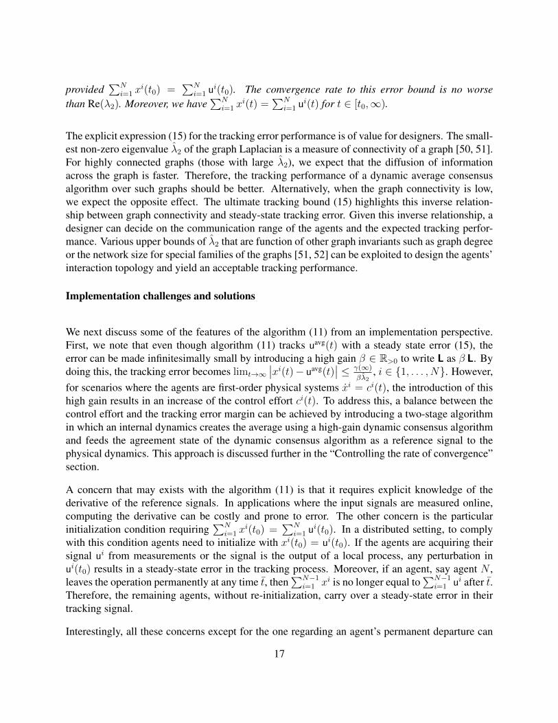
Figure 8: A simple dynamic average consensus based containment and tracking of a team of mobile targets:The triangle robots cooperatively want to contain the moving round robots by forming a formation aroundthe geometric center of the round robots that they are observing. At plot (b), say after 10 s from the startof the operation, one of the triangle robots leaves the team. At plot (c), say after 20 s from the start of theoperation, a new triangle robot joins the group to take over tracking the abandoned round robot.

Example: distributed formation control revisited

We come back to one of the scenarios discussed in the ”Applications of Dynamic Average Consen-sus in Network Systems” to illustrate the properties of algorithm (11) and its alternative implemen-tation (16). Consider a group of four mobile agents (depicted as the triangle robots in Figure 8)whose communication topology is described by a fixed connected undirected ring. The objectiveof these agents is to follow a set of moving targets (depicted as the round robots in Figure 8)in a containment fashion (that is, making sure that they are surrounded as they move around theenvironment). Let

xlT (t) = (t/20)2 + 0.5 sin((0.35 + 0.05l) t+ (5− l)π5

) + 4− 2(l − 1), l ∈ {1, 2, 3, 4}, (18)

be the horizontal position of the set of moving targets (each mobile agent keeps track on onemoving target). The term (t/20)2 in the reference signals (18) represents the component withunbounded derivative but common across all the agents.

To achieve their objective, the group of agents seeks to compute on the fly the geometric centerxT (t) = 1

N

∑Nl=1 x

lT (t) and the associated variance 1

N

∑Nl=1(xl(t) − xT (t))2 determined by the

time-varying position of the moving targets. The agents implement two distributed dynamic aver-age consensus algorithms, one for computing the center, the other for computing the variance, asshown in Figure 9. In this scenario, to illustrate the properties discussed in this section, we haveagent 4 (the green triangle in Figure 8) leave the network 10 s after the beginning of the simulation.Later, 10 s later, a new agent, labeled 5 (the red triangle in Figure 8), joins the network and startsmonitoring the target that the old agent 4 was in charge of.

For simplicity, we focus our simulation on the calculation of the geometric center. For this com-putation, agents implement the algorithm (16) with reference input ui(t) = xiT (t), i ∈ {1, 2, 3, 4}.

20

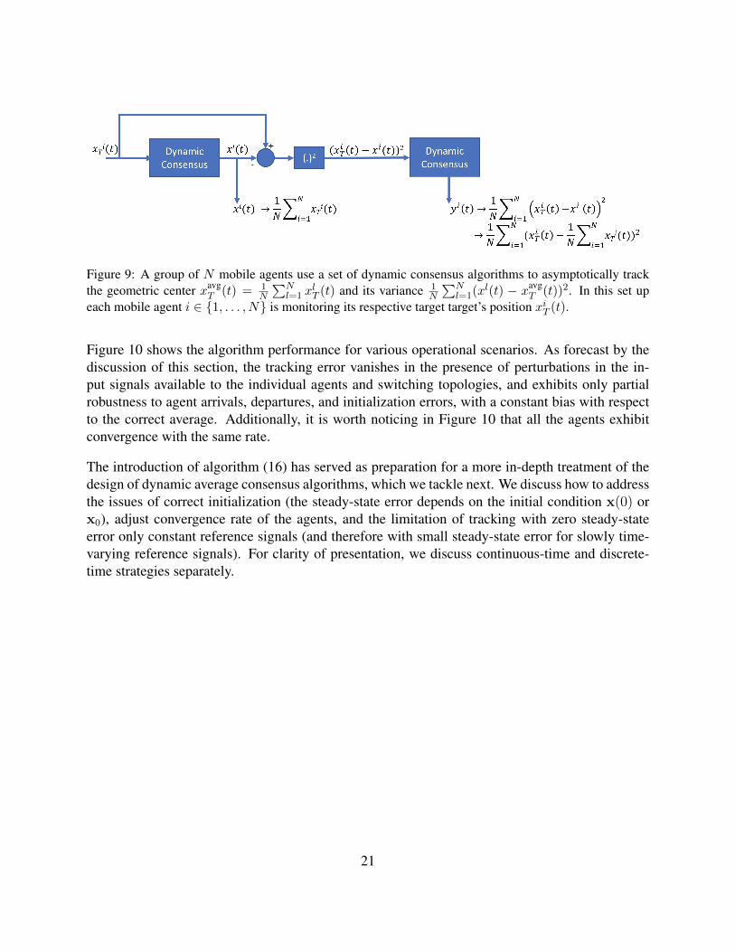
Figure 9: A group of N mobile agents use a set of dynamic consensus algorithms to asymptotically trackthe geometric center xavg

T (t) = 1N

∑Nl=1 x

lT (t) and its variance 1

N

∑Nl=1(xl(t) − xavg

T (t))2. In this set upeach mobile agent i ∈ {1, . . . , N} is monitoring its respective target target’s position xiT (t).

Figure 10 shows the algorithm performance for various operational scenarios. As forecast by thediscussion of this section, the tracking error vanishes in the presence of perturbations in the in-put signals available to the individual agents and switching topologies, and exhibits only partialrobustness to agent arrivals, departures, and initialization errors, with a constant bias with respectto the correct average. Additionally, it is worth noticing in Figure 10 that all the agents exhibitconvergence with the same rate.

The introduction of algorithm (16) has served as preparation for a more in-depth treatment of thedesign of dynamic average consensus algorithms, which we tackle next. We discuss how to addressthe issues of correct initialization (the steady-state error depends on the initial condition x(0) orx0), adjust convergence rate of the agents, and the limitation of tracking with zero steady-stateerror only constant reference signals (and therefore with small steady-state error for slowly time-varying reference signals). For clarity of presentation, we discuss continuous-time and discrete-time strategies separately.

21

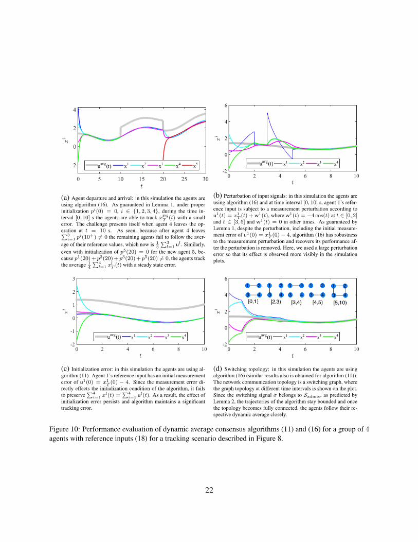
(a) Agent departure and arrival: in this simulation the agents areusing algorithm (16). As guaranteed in Lemma 1, under properinitialization pi(0) = 0, i ∈ {1, 2, 3, 4}, during the time in-terval [0, 10] s the agents are able to track xavg

T (t) with a smallerror. The challenge presents itself when agent 4 leaves the op-eration at t = 10 s. As seen, because after agent 4 leaves∑3i=1 p

i(10+) 6= 0 the remaining agents fail to follow the aver-age of their reference values, which now is 1

3

∑3l=1 u

l. Similarly,even with initialization of p5(20) = 0 for the new agent 5, be-cause p1(20) + p2(20) + p3(20) + p5(20) 6= 0, the agents trackthe average 1

4

∑4l=1 x

lT (t) with a steady state error.

(b) Perturbation of input signals: in this simulation the agents areusing algorithm (16) and at time interval [0, 10] s, agent 1’s refer-ence input is subject to a measurement perturbation according tou1(t) = x1T (t) + w1(t), where w1(t) = −4 cos(t) at t ∈ [0, 2]and t ∈ [3, 5] and w1(t) = 0 in other times. As guaranteed byLemma 1, despite the perturbation, including the initial measure-ment error of u1(0) = x1T (0) − 4, algorithm (16) has robustnessto the measurement perturbation and recovers its performance af-ter the perturbation is removed. Here, we used a large perturbationerror so that its effect is observed more visibly in the simulationplots.

(c) Initialization error: in this simulation the agents are using al-gorithm (11). Agent 1’s reference input has an initial measurementerror of u1(0) = x1T (0) − 4. Since the measurement error di-rectly effects the initialization condition of the algorithm, it failsto preserve

∑4i=1 x

l(t) =∑4i=1 u

l(t). As a result, the effect ofinitialization error persists and algorithm maintains a significanttracking error.

(d) Switching topology: in this simulation the agents are usingalgorithm (16) (similar results also is obtained for algorithm (11)).The network communication topology is a switching graph, wherethe graph topology at different time intervals is shown on the plot.Since the switching signal σ belongs to Sadmis, as predicted byLemma 2, the trajectories of the algorithm stay bounded and oncethe topology becomes fully connected, the agents follow their re-spective dynamic average closely.

Figure 10: Performance evaluation of dynamic average consensus algorithms (11) and (16) for a group of 4agents with reference inputs (18) for a tracking scenario described in Figure 8.

22

Continuous-Time Dynamic Average Consensus Algorithms

In the following, we discuss various continuous-time dynamic average consensus algorithms anddiscuss their performance and robustness guarantees. Table 1 summarizes the arguments of thedriving command of these algorithms in (1) and their special initialization requirements. Someof these algorithms when cast in the form of (1) require access to the derivative of the referencesignals. Similar to the algorithm (11), however, this requirement can be eliminated using alternativeimplementations.

Table 1: Arguments of the driving command in (1) for the reviewed continuous-time dynamic averageconsensus algorithms together with their initialization requirements.

Algorithm (11) (19) (24) (25)

J i(t) {xi(t), u(t)} {xi(t), vi(t), u(t)} {xi(t), zi(t), vi(t),u(t), u(t)}

{xi(t), vi(t),u(t), u(t)}

{Ij(t)}j∈N iout{xj(t)}j∈N iout

{xj(t), vj(t)}j∈N iout{zj(t), vj(t)}j∈N iout

{vi(t)}j∈N ioutInitializationRequirement xi(0)=ui(0) none none

∑Nj=1 v

j(0) = 0

Robustness to initialization and permanent agent dropout

To eliminate the special initialization requirement and to induce robustness with respect to algo-rithm initialization, [53] proposes the following alternative dynamic average consensus algorithm

qi(t) = −N∑j=1

bij (xi − xj), (19a)

xi = −α (xi − ui)−N∑j=1

aij (xi − xj) +N∑j=1

bji (qi − qj) + ui, (19b)

qi(t0), xi(t0) ∈ R, i ∈ {1, . . . , N}, (19c)

where α ∈ R>0. Here, we add ui to (19b) to allow agents to track reference inputs whose deriva-tives have unbounded common components. The necessity of having explicit knowledge of thederivative of reference signals can be removed by using the change of variables pi = xi − ui,i ∈ {1, . . . , N}. In algorithm (19), the agents are allowed to use two different adjacency ma-trices [aij]N×N and [bij]N×N , so that they have an extra degree of freedom to adjust the trackingperformance of the algorithm. The Laplacian matrices associated with adjacency matrices [aij]and [bij] are represented by, respectively, Lp, labeled as proportional Laplacian and LI, labeled asintegral Laplacian. Without loss of generality, to simplify the algorithm we can set LI = βLP, for

23

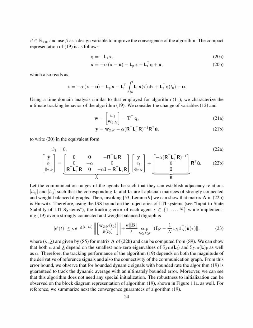
β ∈ R>0, and use β as a design variable to improve the convergence of the algorithm. The compactrepresentation of (19) is as follows

q = −LI x, (20a)

x = −α (x− u)− Lp x + L>I q + u, (20b)

which also reads as

x = −α (x− u)− Lp x− L>I

∫ t

t0

LI x(τ) dτ + L>I q(t0) + u.

Using a time-domain analysis similar to that employed for algorithm (11), we characterize theultimate tracking behavior of the algorithm (19). We consider the change of variables (12) and

w =

[w1

w2:N

]= T> q, (21a)

y = w2:N − α(R>L>I R)−1R>u, (21b)

to write (20) in the equivalent form

w1 = 0, (22a) y˙e1

˙e2:N

=

0 0 −R>LIR0 −α 0

R>L>I R 0 −αI− R>LpR

︸ ︷︷ ︸

A

ye1

e2:N

+

−α(R>L>I R)−1

0I

︸ ︷︷ ︸

B

R>u. (22b)

Let the communication ranges of the agents be such that they can establish adjacency relations[aij] and [bij] such that the corresponding LI and LP are Laplacian matrices of strongly connectedand weight-balanced digraphs. Then, invoking [53, Lemma 9] we can show that matrix A in (22b)is Hurwitz. Therefore, using the ISS bound on the trajectories of LTI systems (see “Input-to-StateStability of LTI Systems”), the tracking error of each agent i ∈ {1, . . . , N} while implement-ing (19) over a strongly connected and weight-balanced digraph is

|ei(t)| ≤κ e−λ (t−t0)

∥∥∥∥[w2:N(t0)e(t0)

]∥∥∥∥+κ‖B‖λ

supt0≤τ≤t

‖(IN −1

N1N1>N)u(τ)‖, (23)

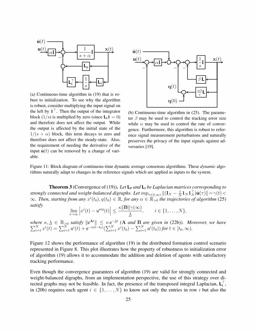
where (κ, λ) are given by (S5) for matrix A of (22b) and can be computed from (S9). We can showthat both κ and λ depend on the smallest non-zero eigenvalues of Sym(LI) and Sym(L)P as wellas α. Therefore, the tracking performance of the algorithm (19) depends on both the magnitude ofthe derivative of reference signals and also the connectivity of the communication graph. From thiserror bound, we observe that for bounded dynamic signals with bounded rate the algorithm (19) isguaranteed to track the dynamic average with an ultimately bounded error. Moreover, we can seethat this algorithm does not need any special initialization. The robustness to initialization can beobserved on the block diagram representation of algorithm (19), shown in Figure 11a, as well. Forreference, we summarize next the convergence guarantees of algorithm (19).

24

αI

u(t)

L>I1

sLI

Lp

1

s+ αI

u(t)

−x(t)

(a) Continuous-time algorithm in (19) that is ro-bust to initialization. To see why the algorithmis robust, consider multiplying the input signal onthe left by 1>. Then the output of the integratorblock (1/s) is multiplied by zero (since LI1 = 0)and therefore does not affect the output. Whilethe output is affected by the initial state of the1/(s + α) block, this term decays to zero andtherefore does not affect the steady-state. Also,the requirement of needing the derivative of theinput u(t) can be removed by a change of vari-able.

αI

u(t)

1

sI

β L

αβsL

q(0)

u(t) x(t)

−−

q(t)

−

(b) Continuous-time algorithm in (25). The parame-ter β may be used to control the tracking error sizewhile α may be used to control the rate of conver-gence. Furthermore, this algorithm is robust to refer-ence signal measurement perturbations and naturallypreserves the privacy of the input signals against ad-versaries [19].

Figure 11: Block diagram of continuous-time dynamic average consensus algorithms. These dynamic algo-rithms naturally adapt to changes in the reference signals which are applied as inputs to the system.

Theorem 3 (Convergence of (19)). Let LP and LI be Laplacian matrices corresponding tostrongly connected and weight-balanced digraphs. Let supτ∈[t,∞) ‖(IN − 1

N1N1>N)u(τ)‖=γ(t)<

∞. Then, starting from any xi(t0), q(t0) ∈ R, for any α ∈ R>0 the trajectories of algorithm (25)satisfy

limt→∞

∣∣∣xi(t)− uavg(t)∣∣∣ ≤ κ‖B‖γ(∞)

λ, i ∈ {1, . . . , N},

where κ, λ ∈ R>0 satisfy ‖eAt‖ ≤ κ e−λt (A and B are given in (22b)). Moreover, we have∑Ni=1 x

i(t) =∑N

i=1 ui(t) + e−α(t−t0)(

∑Ni=1 x

i(t0)−∑N

i=1 ui(t0)) for t ∈ [t0,∞).

Figure 12 shows the performance of algorithm (19) in the distributed formation control scenariorepresented in Figure 8. This plot illustrates how the property of robustness to initialization errorof algorithm (19) allows it to accommodate the addition and deletion of agents with satisfactorytracking performance.

Even though the convergence guarantees of algorithm (19) are valid for strongly connected andweight-balanced digraphs, from an implementation perspective, the use of this strategy over di-rected graphs may not be feasible. In fact, the presence of the transposed integral Laplacian, L>I ,in (20b) requires each agent i ∈ {1, . . . , N} to know not only the entries in row i but also the

25

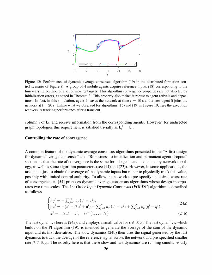
Figure 12: Performance of dynamic average consensus algorithm (19) in the distributed formation con-trol scenario of Figure 8. A group of 4 mobile agents acquire reference inputs (18) corresponding to thetime-varying position of a set of moving targets. This algorithm convergence properties are not affected byinitialization errors, as stated in Theorem 3. This property also makes it robust to agent arrivals and depar-tures. In fact, in this simulation, agent 4 leaves the network at time t = 10 s and a new agent 5 joins thenetwork at t = 20 s. Unlike what we observed for algorithms (16) and (19) in Figure 10, here the executionrecovers its tracking performance after a transient.

column i of LI, and receive information from the corresponding agents. However, for undirectedgraph topologies this requirement is satisfied trivially as L>I = LI.

Controlling the rate of convergence

A common feature of the dynamic average consensus algorithms presented in the ”A first designfor dynamic average consensus” and ”Robustness to initialization and permanent agent dropout”sections is that the rate of convergence is the same for all agents and is dictated by network topol-ogy, as well as some algorithm parameters (see (14) and (23)). However, in some applications, thetask is not just to obtain the average of the dynamic inputs but rather to physically track this value,possibly with limited control authority. To allow the network to pre-specify its desired worst rateof convergence, β, [54] proposes dynamic average consensus algorithms whose design incorpo-rates two time scales. The 1st-Order-Input Dynamic Consensus (FOI-DC ) algorithm is describedas follows {

ε qi = −∑N

j=1 bij(zi − zj),

ε zi = −(zi + β ui + ui)−∑N

j=1 aij(zi − zj) +

∑Nj=1 bji(q

i − qj),(24a)

xi = −β xi − zi, i ∈ {1, . . . , N} (24b)

The fast dynamics here is (24a), and employs a small value for ε ∈ R>0. The fast dynamics, whichbuilds on the PI algorithm (19), is intended to generate the average of the sum of the dynamicinput and its first derivative. The slow dynamics (24b) then uses the signal generated by the fastdynamics to track the average of the reference signal across the network at a pre-specified smallerrate β ∈ R>0. The novelty here is that these slow and fast dynamics are running simultaneously

26

and, thus, there is no need to wait for convergence of the fast dynamics and then take slow stepstowards the input average.

Similar to the dynamic average consensus algorithm (19), (24) does not require any specific ini-tialization. The technical approach used in [54] to study the convergence of (24) is based onsingular perturbation theory [55, Chapter 11], which results in a guaranteed convergence to anε-neighborhood of uavg(t) for small values of ε ∈ R>0.

Using time-domain analysis, we can make more precise the information about the ultimate trackingbehavior of algorithm(19). For convenience, we apply the change of variables (12), (21a) alongwith y = w2:N − (R>L>I R)−1R>(βu+ u), and ez = T>(z + β 1

N

∑Nj=1 u

j1N + 1N

∑Nj=1 u

j1N) towrite the FOI-DC algorithm as follows

w1 = 0,[yez

]=ε−1

0[0 −R>LIR

][0

R>L>I R

] [−1 0

0 −I− R>LpR

]︸ ︷︷ ︸

A

[yez

]+

−(R>L>I R)−1[0(N−1)×1 IN−1

][[1 01×N−1

]0(N−1)×N

] ︸ ︷︷ ︸

B

f(t),

e = −β e− ez,

where f(t) = T>(β u + u). Using the ISS bound on the trajectories of LTI systems, see “Input-to-State Stability of LTI Systems”, the tracking error of each agent i ∈ {1, . . . , N} while implement-ing FOI-DC algorithm with an ε ∈ R>0 is as follows, i ∈ {1, . . . , N},

|ei(t)| ≤ e−β (t−t0)|ei(t0)|+ κ

βsupt0≤τ≤t

(e−ε

−1λ (t−t0)∥∥∥ [y(t0)

ez(t0)

] ∥∥∥+ε‖B‖λ

supt0≤τ≤t

‖β u(τ) + u(τ)‖),

where ‖eA t‖ ≤ κe−λ t. From this error bound, we observe that for dynamic signals with boundedfirst and second derivatives FOI-DC algorithm is guaranteed to track the dynamic average withan ultimately bounded error. This tracking error can be made small using a small ε ∈ R>0. Useof small ε ∈ R>0 also results in dynamics (25a) to have a higher decay rate. Therefore, thedominant rate of convergence of FOI-DC algorithm is determined by β, which can be pre-specifiedregardless of the interaction topology. Moreover, β can be used to regulate the control effort of theintegrator dynamics xi = ci(t), i ∈ {1, . . . , N} while maintaining a good tracking error via theuse of small ε ∈ R>0.

An alternative algorithm for directed graphs

As observed, the algorithm (19) is not implementable over directed graphs, since it requires infor-mation exchange with both in- and out-neighbors, and these sets are generally different. In [19] au-thors proposed a modified proportional and integral agreement feedback dynamic average consen-sus algorithm whose implementation does not require the agents to know their respective columns

27

of the Laplacian. This algorithm is

qi = αβ∑N

j=1aij(x

i − xj), (25a)

xi = −α(xi − ui)−β∑N

j=1aij(x

i − xj)−qi + ui, (25b)

xi(t0), qi(t0) ∈ R s.t.∑N

j=1qj(t0) = 0, (25c)

i ∈ {1, . . . , N}, where α, β ∈ R>0. Algorithm (25) in compact form can be equivalently writtenas

x = −α (x− u)− β Lx− αβ∫ t

t0

Lx(τ) dτ − q(t0) + u,

which demonstrates the proportional and integral agreement feedback structure of this algorithm.As we did for algorithm (11), we can use a change of variables pi = ui−xi, to write this algorithmin a form whose implementation does not require the knowledge of the derivative of the referencesignals.

We should point out an interesting connection between algorithms (25) and (16). If we writethe transfer function from the reference input to the tracking error state (25), there is a pole-zerocancellation which reduces the algorithm (25) to (11) and (16). Despite this close relationship,there are some subtle differences. For example, unlike (11), algorithm (25) enjoys robustness toreference signal measurement perturbations and naturally preserves the privacy of the input ofeach agent against adversaries: specifically [19], an adversary with access to the time history of allnetwork communication messages cannot uniquely reconstruct the reference signal of any agent,which is not the case for algorithm (16).

Figure 11b shows the block diagram representation of this algorithm. The next result states theconvergence properties of (25). We refer the reader to [19] for the proof of this statement whichis established using the time domain analysis we implemented to analyze the algorithms we havereviewed so far.

Theorem 4 (Convergence of (25) over strongly connected and weight-balanced digraphsfor dynamic input signals [19]). Let G be a strongly connected and weight-balanced digraph. Letsupτ∈[t,∞) ‖(IN − 1

N1N1>N)u(τ)‖ = γ(t) < ∞. Then, for any α, β ∈ R>0, the trajectories of

algorithm (25) satisfy

limt→∞

∣∣∣xi(t)− uavg(t)∣∣∣ ≤ γ(∞)

βλ2

, i ∈ {1, . . . , N}. (26)

provided∑N

j=1 qj(t0) = 0. The convergence rate to the error bound is min{α, β Re(λ2)}.

The inverse relation between β and the tracking error in (26) indicates that we can use the parameterβ to control the tracking error size, while α can be used to control the rate of convergence.

28

Discrete-Time Dynamic Average Consensus Algorithms

While the continuous-time dynamic average consensus algorithms described in the previous sec-tion are amenable to elegant and relatively simple analysis, implementing these algorithms on prac-tical cyber-physical systems requires continuous communication between agents. This requirementis not feasible in practice due to constraints on the communication bandwidth. To address this is-sue, we study here discrete-time dynamic average consensus algorithms where the communicationamong agents occurs only at discrete time steps.

The main difference between continuous-time and discrete-time dynamic average consensus al-gorithms is the rate at which their estimates converge to the average of the reference signals. Incontinuous time, the parameters may be scaled to achieve any desired convergence rate, while indiscrete time the parameters must be carefully chosen to ensure convergence. The problem of op-timizing the convergence rate has received significant attention in the literature [56, 57, 58, 59, 60,61, 62, 63, 64, 65]. Here, we give a simple method using root locus techniques for choosing theparameters in order to optimize the convergence rate. We also show how to further accelerate theconvergence by introducing extra dynamics into the dynamic average consensus algorithm.

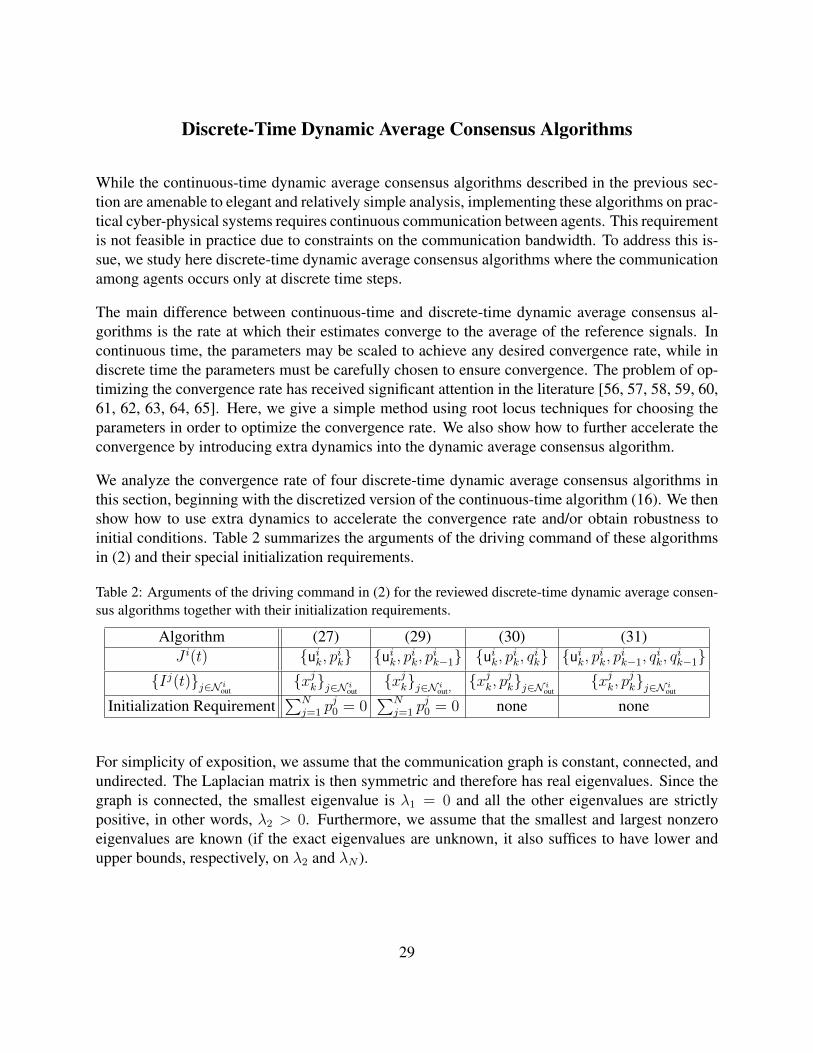
We analyze the convergence rate of four discrete-time dynamic average consensus algorithms inthis section, beginning with the discretized version of the continuous-time algorithm (16). We thenshow how to use extra dynamics to accelerate the convergence rate and/or obtain robustness toinitial conditions. Table 2 summarizes the arguments of the driving command of these algorithmsin (2) and their special initialization requirements.

Table 2: Arguments of the driving command in (2) for the reviewed discrete-time dynamic average consen-sus algorithms together with their initialization requirements.

Algorithm (27) (29) (30) (31)J i(t) {uik, pik} {uik, pik, pik−1} {uik, pik, qik} {uik, pik, pik−1, q

ik, q

ik−1}

{Ij(t)}j∈N iout{xjk}j∈N iout

{xjk}j∈N iout,{xjk, p

jk}j∈N iout

{xjk, pjk}j∈N iout

Initialization Requirement∑N

j=1 pj0 = 0

∑Nj=1 p

j0 = 0 none none

For simplicity of exposition, we assume that the communication graph is constant, connected, andundirected. The Laplacian matrix is then symmetric and therefore has real eigenvalues. Since thegraph is connected, the smallest eigenvalue is λ1 = 0 and all the other eigenvalues are strictlypositive, in other words, λ2 > 0. Furthermore, we assume that the smallest and largest nonzeroeigenvalues are known (if the exact eigenvalues are unknown, it also suffices to have lower andupper bounds, respectively, on λ2 and λN ).

29

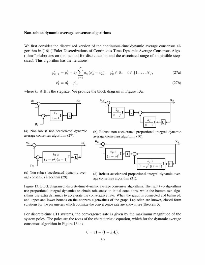
Non-robust dynamic average consensus algorithms

We first consider the discretized version of the continuous-time dynamic average consensus al-gorithm in (16) (“Euler Discretizations of Continuous-Time Dynamic Average Consensus Algo-rithms” elaborates on the method for discretization and the associated range of admissible step-sizes). This algorithm has the iterations

pik+1 = pik + kI

N∑j=1

aij(xik − x

jk), pi0 ∈ R, i ∈ {1, . . . , N}, (27a)

xik = uik − pik, (27b)

where kI ∈ R is the stepsize. We provide the block diagram in Figure 13a.

kIz − 1

I L

p0

uk xk

−

(a) Non-robust non-accelerated dynamicaverage consensus algorithm (27).

kpz − ρ

I L

kIz − 1

I L

uk

−xk

(b) Robust non-accelerated proportional-integral dynamicaverage consensus algorithm (30).

kI z

(z − ρ2)(z − 1)I L

p0

uk xk

−

(c) Non-robust accelerated dynamic aver-age consensus algorithm (29).

kp z

(z − ρ)2I L

kI z

(z − ρ2)(z − 1)I L

uk

−xk

(d) Robust accelerated proportional-integral dynamic aver-age consensus algorithm (31).

Figure 13: Block diagram of discrete-time dynamic average consensus algorithms. The right two algorithmsuse proportional-integral dynamics to obtain robustness to initial conditions, while the bottom two algo-rithms use extra dynamics to accelerate the convergence rate. When the graph is connected and balanced,and upper and lower bounds on the nonzero eigenvalues of the graph Laplacian are known, closed-formsolutions for the parameters which optimize the convergence rate are known; see Theorem 5.

For discrete-time LTI systems, the convergence rate is given by the maximum magnitude of thesystem poles. The poles are the roots of the characteristic equation, which for the dynamic averageconsensus algorithm in Figure 13a is

0 = zI− (I− kIL).

30

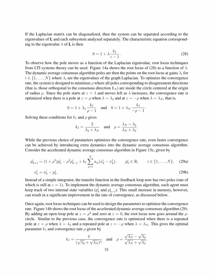
If the Laplacian matrix can be diagonalized, then the system can be separated according to theeigenvalues of L and each subsystem analyzed separately. The characteristic equation correspond-ing to the eigenvalue λ of L is then

0 = 1 + λkI

z − 1. (28)

To observe how the pole moves as a function of the Laplacian eigenvalue, root locus techniquesfrom LTI systems theory can be used. Figure 14a shows the root locus of (28) as a function of λ.The dynamic average consensus algorithm poles are then the points on the root locus at gains λi fori ∈ {1, . . . , N} where λi are the eigenvalues of the graph Laplacian. To optimize the convergencerate, the system is designed to minimize ρwhere all poles corresponding to disagreement directions(that is, those orthogonal to the consensus direction 1N ) are inside the circle centered at the originof radius ρ. Since the pole starts at z = 1 and moves left as λ increases, the convergence rate isoptimized when there is a pole at z = ρ when λ = λ2 and at z = −ρ when λ = λN , that is,

0 = 1 + λ2kI

ρ− 1and 0 = 1 + λN

kI−ρ− 1

.

Solving these conditions for kI and ρ gives

kI =2

λ2 + λNand ρ =

λN − λ2

λN + λ2

.

While the previous choice of parameters optimizes the convergence rate, even faster convergencecan be achieved by introducing extra dynamics into the dynamic average consensus algorithm.Consider the accelerated dynamic average consensus algorithm in Figure 13c, given by

pik+1 = (1 + ρ2)pik − ρ2pik−1 + kI

N∑j=1

aij(xik − x

jk), pi0 ∈ R, i ∈ {1, . . . , N}, (29a)

xik = uik − pik. (29b)

Instead of a simple integrator, the transfer function in the feedback loop now has two poles (one ofwhich is still at z = 1). To implement the dynamic average consensus algorithm, each agent mustkeep track of two internal state variables (pik and pik−1). This small increase in memory, however,can result in a significant improvement in the rate of convergence, as discussed below.

Once again, root locus techniques can be used to design the parameters to optimize the convergencerate. Figure 14b shows the root locus of the accelerated dynamic average consensus algorithm (29).By adding an open-loop pole at z = ρ2 and zero at z = 0, the root locus now goes around the ρ-circle. Similar to the previous case, the convergence rate is optimized when there is a repeatedpole at z = ρ when λ = λ2 and a repeated pole at z = −ρ when λ = λN . This gives the optimalparameter kI and convergence rate ρ given by

kI =4

(√λ2 +

√λN)2

and ρ =

√λN −

√λ2√

λN +√λ2

.

31

−1 1

ρT

Re(z)

Im(z)

(a) Non-accelerated dynamic average consensusalgorithm in Figure 13a.

−1 ρ2 1

ρT

Re(z)

Im(z)

(b) Accelerated dynamic average consensus al-gorithm in Figure 13c.

Figure 14: Root locus design of dynamic average consensus algorithms. The dynamic average consensusalgorithm poles are the points on the root locus at gains λi for i ∈ {1, . . . , N} where λi are the eigenvaluesof the graph Laplacian. To optimize the convergence rate, the parameters are chosen to minimize ρ such thatall poles corresponding to eigenvalues λi for i ∈ {2, . . . , N} are inside the circle centered at the origin ofradius ρ. Then the dynamic average consensus algorithm converges linearly with rate ρ.

The convergence rate of both the standard (Eq. (27)) and accelerated (Eq. (29)) versions of thedynamic average consensus algorithm are plotted in Figure 15 as a function of the ratio λ2/λN .

Robust dynamic average consensus algorithms

While the previous dynamic average consensus algorithms are not robust to initial conditions,we can also use root locus techniques to optimize the convergence rate of dynamic average con-sensus algorithms that are robust to initial conditions. Consider the discrete-time version of theproportional-integral estimator from (19) whose iterations are given by

qik+1 = ρ qik + kp

N∑j=1

aij((xik − x

jk) + (pik − p

jk)), (30a)

pik+1 = pik + kI

N∑j=1

aij(xik − x

jk), (30b)

xik = uik − qik, pi0, qi0 ∈ R, i ∈ {1, . . . , N} (30c)

with parameters ρ, kp, kI ∈ R. The block diagram of this algorithm is shown in Figure 13b.

Since the dynamic average consensus algorithms (27) and (29) have only one Laplacian blockin the block diagram, the resulting root loci are linear in the Laplacian eigenvalues. For the

32

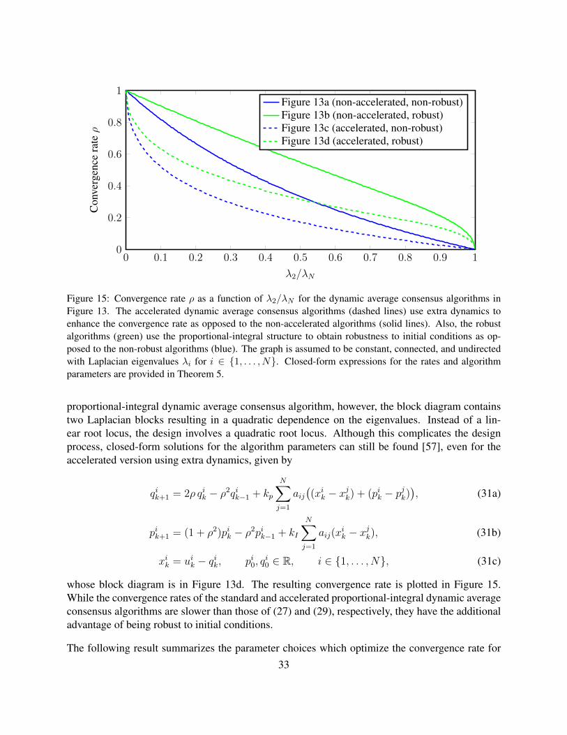
0 0.1 0.2 0.3 0.4 0.5 0.6 0.7 0.8 0.9 10

0.2

0.4

0.6

0.8

1

λ2/λN

Con

verg

ence

rateρ

Figure 13a (non-accelerated, non-robust)Figure 13b (non-accelerated, robust)Figure 13c (accelerated, non-robust)Figure 13d (accelerated, robust)

Figure 15: Convergence rate ρ as a function of λ2/λN for the dynamic average consensus algorithms inFigure 13. The accelerated dynamic average consensus algorithms (dashed lines) use extra dynamics toenhance the convergence rate as opposed to the non-accelerated algorithms (solid lines). Also, the robustalgorithms (green) use the proportional-integral structure to obtain robustness to initial conditions as op-posed to the non-robust algorithms (blue). The graph is assumed to be constant, connected, and undirectedwith Laplacian eigenvalues λi for i ∈ {1, . . . , N}. Closed-form expressions for the rates and algorithmparameters are provided in Theorem 5.

proportional-integral dynamic average consensus algorithm, however, the block diagram containstwo Laplacian blocks resulting in a quadratic dependence on the eigenvalues. Instead of a lin-ear root locus, the design involves a quadratic root locus. Although this complicates the designprocess, closed-form solutions for the algorithm parameters can still be found [57], even for theaccelerated version using extra dynamics, given by

qik+1 = 2ρ qik − ρ2qik−1 + kp

N∑j=1

aij((xik − x

jk) + (pik − p

jk)), (31a)

pik+1 = (1 + ρ2)pik − ρ2pik−1 + kI

N∑j=1

aij(xik − x

jk), (31b)

xik = uik − qik, pi0, qi0 ∈ R, i ∈ {1, . . . , N}, (31c)

whose block diagram is in Figure 13d. The resulting convergence rate is plotted in Figure 15.While the convergence rates of the standard and accelerated proportional-integral dynamic averageconsensus algorithms are slower than those of (27) and (29), respectively, they have the additionaladvantage of being robust to initial conditions.

The following result summarizes the parameter choices which optimize the convergence rate for33

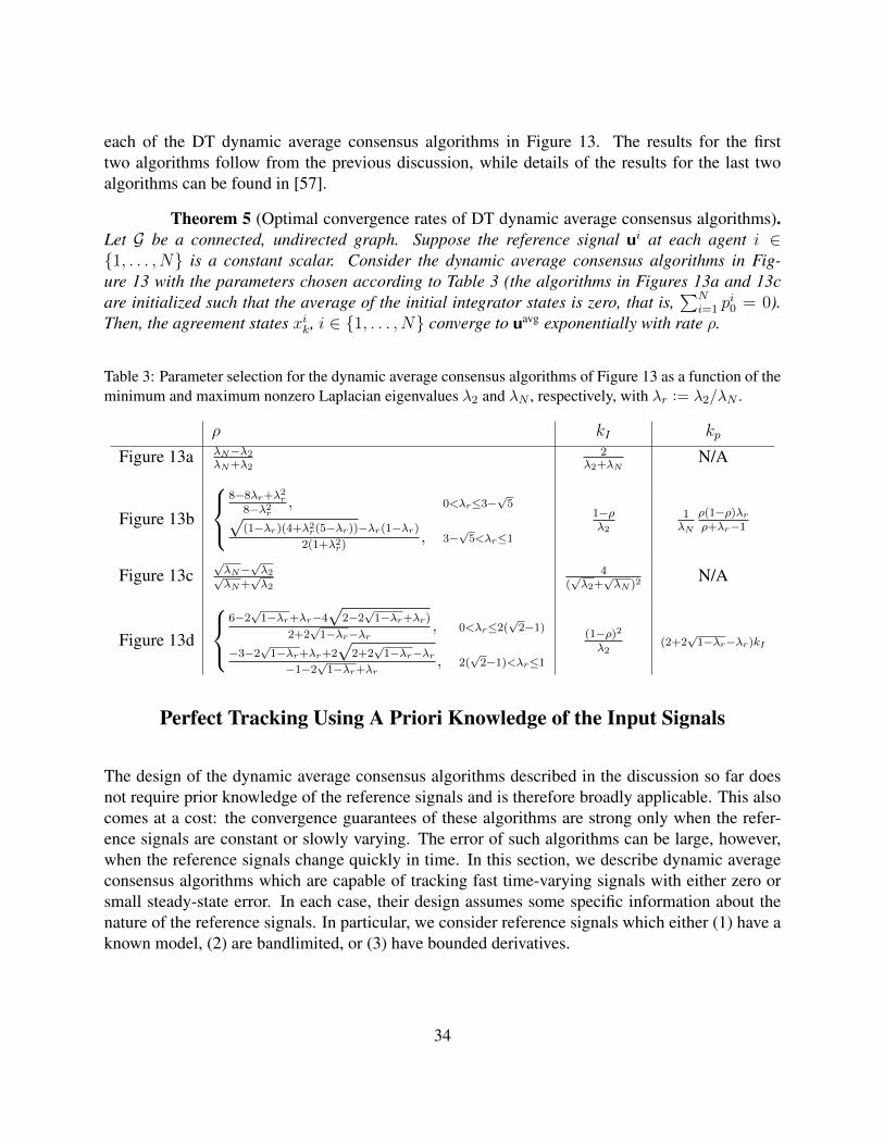
each of the DT dynamic average consensus algorithms in Figure 13. The results for the firsttwo algorithms follow from the previous discussion, while details of the results for the last twoalgorithms can be found in [57].

Theorem 5 (Optimal convergence rates of DT dynamic average consensus algorithms).Let G be a connected, undirected graph. Suppose the reference signal ui at each agent i ∈{1, . . . , N} is a constant scalar. Consider the dynamic average consensus algorithms in Fig-ure 13 with the parameters chosen according to Table 3 (the algorithms in Figures 13a and 13care initialized such that the average of the initial integrator states is zero, that is,

∑Ni=1 p

i0 = 0).

Then, the agreement states xik, i ∈ {1, . . . , N} converge to uavg exponentially with rate ρ.

Table 3: Parameter selection for the dynamic average consensus algorithms of Figure 13 as a function of theminimum and maximum nonzero Laplacian eigenvalues λ2 and λN , respectively, with λr := λ2/λN .

ρ kI kp

Figure 13a λN−λ2λN+λ2

2λ2+λN

N/A

Figure 13b

8−8λr+λ2r

8−λ2r, 0<λr≤3−

√5

√(1−λr)(4+λ2r(5−λr))−λr(1−λr)

2(1+λ2r), 3−

√5<λr≤1

1−ρλ2

1λN

ρ(1−ρ)λrρ+λr−1

Figure 13c√λN−

√λ2√

λN+√λ2

4(√λ2+√λN )2

N/A

Figure 13d

6−2√

1−λr+λr−4√

2−2√

1−λr+λr)2+2√

1−λr−λr, 0<λr≤2(

√2−1)

−3−2√

1−λr+λr+2√

2+2√

1−λr−λr−1−2

√1−λr+λr

, 2(√

2−1)<λr≤1

(1−ρ)2

λ2(2+2

√1−λr−λr)kI

Perfect Tracking Using A Priori Knowledge of the Input Signals

The design of the dynamic average consensus algorithms described in the discussion so far doesnot require prior knowledge of the reference signals and is therefore broadly applicable. This alsocomes at a cost: the convergence guarantees of these algorithms are strong only when the refer-ence signals are constant or slowly varying. The error of such algorithms can be large, however,when the reference signals change quickly in time. In this section, we describe dynamic averageconsensus algorithms which are capable of tracking fast time-varying signals with either zero orsmall steady-state error. In each case, their design assumes some specific information about thenature of the reference signals. In particular, we consider reference signals which either (1) have aknown model, (2) are bandlimited, or (3) have bounded derivatives.

34

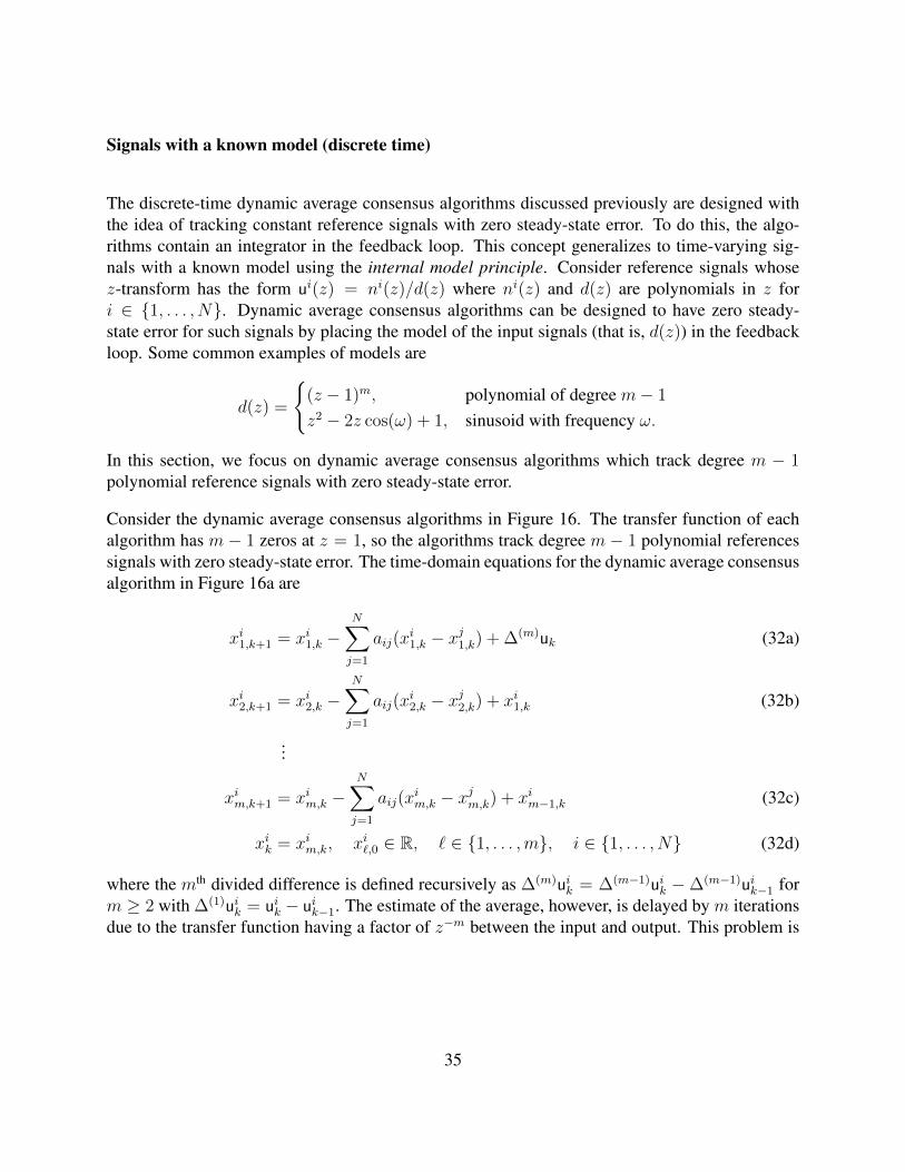
Signals with a known model (discrete time)

The discrete-time dynamic average consensus algorithms discussed previously are designed withthe idea of tracking constant reference signals with zero steady-state error. To do this, the algo-rithms contain an integrator in the feedback loop. This concept generalizes to time-varying sig-nals with a known model using the internal model principle. Consider reference signals whosez-transform has the form ui(z) = ni(z)/d(z) where ni(z) and d(z) are polynomials in z fori ∈ {1, . . . , N}. Dynamic average consensus algorithms can be designed to have zero steady-state error for such signals by placing the model of the input signals (that is, d(z)) in the feedbackloop. Some common examples of models are

d(z) =

{(z − 1)m, polynomial of degree m− 1

z2 − 2z cos(ω) + 1, sinusoid with frequency ω.

In this section, we focus on dynamic average consensus algorithms which track degree m − 1polynomial reference signals with zero steady-state error.

Consider the dynamic average consensus algorithms in Figure 16. The transfer function of eachalgorithm has m − 1 zeros at z = 1, so the algorithms track degree m − 1 polynomial referencessignals with zero steady-state error. The time-domain equations for the dynamic average consensusalgorithm in Figure 16a are

xi1,k+1 = xi1,k −N∑j=1

aij(xi1,k − x

j1,k) + ∆(m)uk (32a)

xi2,k+1 = xi2,k −N∑j=1

aij(xi2,k − x

j2,k) + xi1,k (32b)

...

xim,k+1 = xim,k −N∑j=1

aij(xim,k − x

jm,k) + xim−1,k (32c)

xik = xim,k, xi`,0 ∈ R, ` ∈ {1, . . . ,m}, i ∈ {1, . . . , N} (32d)

where the mth divided difference is defined recursively as ∆(m)uik = ∆(m−1)uik −∆(m−1)uik−1 form ≥ 2 with ∆(1)uik = uik − uik−1. The estimate of the average, however, is delayed by m iterationsdue to the transfer function having a factor of z−m between the input and output. This problem is

35

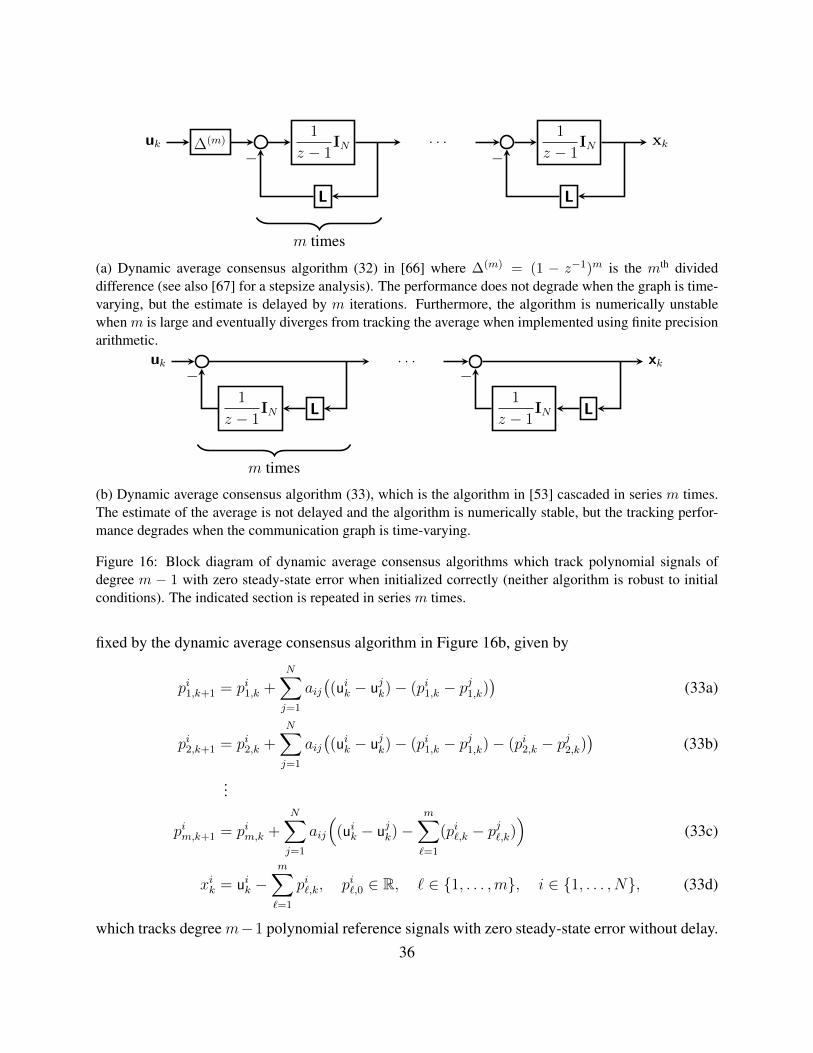
uk ∆(m)1

z − 1IN

L

−. . . 1

z − 1IN

L

xk−

m times

(a) Dynamic average consensus algorithm (32) in [66] where ∆(m) = (1 − z−1)m is the mth divideddifference (see also [67] for a stepsize analysis). The performance does not degrade when the graph is time-varying, but the estimate is delayed by m iterations. Furthermore, the algorithm is numerically unstablewhen m is large and eventually diverges from tracking the average when implemented using finite precisionarithmetic.

uk

1

z − 1IN L

−. . .

1

z − 1IN L

xk−

m times

(b) Dynamic average consensus algorithm (33), which is the algorithm in [53] cascaded in series m times.The estimate of the average is not delayed and the algorithm is numerically stable, but the tracking perfor-mance degrades when the communication graph is time-varying.

Figure 16: Block diagram of dynamic average consensus algorithms which track polynomial signals ofdegree m − 1 with zero steady-state error when initialized correctly (neither algorithm is robust to initialconditions). The indicated section is repeated in series m times.

fixed by the dynamic average consensus algorithm in Figure 16b, given by

pi1,k+1 = pi1,k +N∑j=1

aij((uik − ujk)− (pi1,k − p

j1,k))

(33a)

pi2,k+1 = pi2,k +N∑j=1

aij((uik − ujk)− (pi1,k − p

j1,k)− (pi2,k − p

j2,k))

(33b)

...

pim,k+1 = pim,k +N∑j=1

aij

((uik − ujk)−

m∑`=1

(pi`,k − pj`,k))

(33c)

xik = uik −m∑`=1

pi`,k, pi`,0 ∈ R, ` ∈ {1, . . . ,m}, i ∈ {1, . . . , N}, (33d)

which tracks degree m−1 polynomial reference signals with zero steady-state error without delay.36

Note, however, that the communication graph is assumed to be constant in order to use frequencydomain arguments; while the output of the dynamic average consensus algorithm in Figure 16ais delayed, it also has nice tracking properties when the communication graph is time-varyingwhereas the dynamic average consensus algorithm in Figure 16b does not.

To track degree m − 1 polynomial reference signals, each dynamic average consensus algorithmin Figure 16 cascades m dynamic average consensus algorithms, each with a pole at z = 1 inthe feedback loop. The dynamic average consensus algorithm (27) is cascaded in Figure 16b, butany of the dynamic average consensus algorithms from the previous section could also be used.For example, the proportional-integral dynamic average consensus algorithm could be cascaded mtimes to track degree m− 1 polynomial reference signals with zero steady-state error independentof the initial conditions.

In general, reference signals with model d(z) can be tracked with zero steady-state error by cas-cading simple dynamic average consensus algorithms, each of which tracks a factor of d(z). Inparticular, suppose d(z) = d1(z) d2(z) . . . dm(z). Then m dynamic average consensus algorithmscan be cascaded where the ith component contains the model di(z) for i = 1, . . . ,m. Alternatively,a single dynamic average consensus algorithm can be designed which contains the entire modeld(z). This approach using an internal model version of the proportional-integral dynamic averageconsensus algorithm is designed in [68] in both continuous and discrete time.

In many practical applications, the exact model of the reference signals is unknown. However, it isshown in [69] that a frequency estimator can be used in conjunction with an internal model dynamicaverage consensus algorithm to still achieve zero steady-state error. In particular, the frequency ofthe reference signals is estimated such that the estimate converges to the actual frequency. Thistime-varying estimate of the frequency is then used in place of the true frequency to design thefeedback dynamic average consensus algorithm [69].

Bandlimited signals (discrete time)

In order to use algorithms designed using the model of the reference signals, the signals must becomposed of a finite number of known frequencies. When either the frequencies are unknown orthere are infinitely many frequencies, dynamic average consensus algorithms can still be designedif the reference signals are bandlimited. In this case, feedforward dynamic average consensusalgorithm designs can be used to achieve arbitrarily small steady-state error.

For our discussion here, we assume that the reference signals are bandlimited with known cutofffrequency. In particular, let Ui(z) be the z-transform of the ith reference signal {uik}. Then Ui(z)is bandlimited with cutoff frequency θc if |Ui(exp(jθ))| = 0 for all θ ∈ (θc, π].

Consider the dynamic average consensus algorithm in Figure 17. The reference signals are passedthrough a prefilter h(z) and then multiplied m times by the consensus matrix I − L with a delay

37

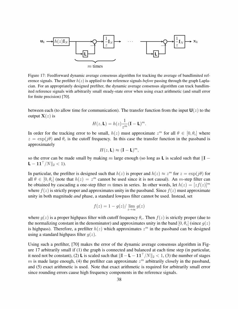
uk h(z)IN

L

1

zIN−

. . .

L

1

zIN xk

−

m times

Figure 17: Feedforward dynamic average consensus algorithm for tracking the average of bandlimited ref-erence signals. The prefilter h(z) is applied to the reference signals before passing through the graph Lapla-cian. For an appropriately designed prefilter, the dynamic average consensus algorithm can track bandlim-ited reference signals with arbitrarily small steady-state error when using exact arithmetic (and small errorfor finite precision) [70].

between each (to allow time for communication). The transfer function from the input U(z) to theoutput X(z) is

H(z,L) = h(z)1

zm(I− L)m.

In order for the tracking error to be small, h(z) must approximate zm for all θ ∈ [0, θc] wherez = exp(jθ) and θc is the cutoff frequency. In this case the transfer function in the passband isapproximately

H(z,L) ≈ (I− L)m,

so the error can be made small by making m large enough (so long as L is scaled such that ‖I −L− 11>/N‖2 < 1).

In particular, the prefilter is designed such that h(z) is proper and h(z) ≈ zm for z = exp(jθ) forall θ ∈ [0, θc] (note that h(z) = zm cannot be used since it is not causal). An m-step filter canbe obtained by cascading a one-step filter m times in series. In other words, let h(z) = [zf(z)]m

where f(z) is strictly proper and approximates unity in the passband. Since f(z) must approximateunity in both magnitude and phase, a standard lowpass filter cannot be used. Instead, set

f(z) = 1− g(z)/ limz→∞

g(z)

where g(z) is a proper highpass filter with cutoff frequency θc. Then f(z) is strictly proper (due tothe normalizing constant in the denominator) and approximates unity in the band [0, θc] (since g(z)is highpass). Therefore, a prefilter h(z) which approximates zm in the passband can be designedusing a standard highpass filter g(z).

Using such a prefilter, [70] makes the error of the dynamic average consensus algorithm in Fig-ure 17 arbitrarily small if (1) the graph is connected and balanced at each time step (in particular,it need not be constant), (2) L is scaled such that ‖I− L− 11>/N‖2 < 1, (3) the number of stagesm is made large enough, (4) the prefilter can approximate zm arbitrarily closely in the passband,and (5) exact arithmetic is used. Note that exact arithmetic is required for arbitrarily small errorsince rounding errors cause high frequency components in the reference signals.

38

Signals with bounded derivatives (continuous time)

Stronger tracking results can be obtained using algorithms implemented in continuous time. Here,we present a set of continuous-time dynamic average consensus algorithms which are capable oftracking time-varying reference signals whose derivatives are bounded with zero error in finite time.For simplicity, we assume that the communication graph is constant, connected, and undirected.Also, the reference signals are assumed to be differentiable with bounded derivatives.

In discrete time, zero steady-state error is obtained by placing the internal model of the referencesignals in the feedback loop. This provides infinite loop gain at the frequencies contained in the ref-erence signals. In continuous time, however, the discontinuous signum function sgn can be used inthe feedback loop to provide ‘infinite’ loop gain over all frequencies, so no model of the referencesignals is required. Furthermore, such continuous-time dynamic average consensus algorithms arecapable of achieving zero error tracking in finite time as opposed to the exponential convergenceachieved by discrete-time dynamic average consensus algorithms. One such algorithm is describedin [71] as

xi = ui − kp∑j∈N iout

sgn(xi(t)− xj(t)), i ∈ {1, . . . , N}, (34a)

∑N

i=1xi(0) =

∑N

i=1ui(0). (34b)

The block diagram representation in Figure 18a indicates that this algorithm applies sgn in thefeedback loop. Under the given assumptions, using a sliding mode argument, the feedback gain kpcan be selected to guarantee zero error tracking in finite time provided that an upper bound γ ofthe form supτ∈[0,∞) ‖u(τ)‖ = γ < ∞ is known [71]. The dynamic consensus algorithm (34) canalso be implemented without derivative information of the reference signals in an equivalent wayas

pi = kp∑j∈N iout

sgn(xi − xj),∑N

j=1pj(0) = 0, (35a)

xi = ui − pi, i ∈ {1, . . . , N}. (35b)

The corresponding block diagram is shown in Figure 18b.

It is simple to see from the block diagram of Figure 18a why (34) is not robust to initial conditions;the integrator state is directly connected to the output and therefore affects the steady-state outputin the consensus direction. This issue is addressed by the dynamic average consensus algorithm inFigure 18c, given by

pi = kp sgn( ∑j∈N iout

(xi − xj)), pi(0) ∈ R, (36a)

xi = ui −∑j∈N iout

(pi − pj), i ∈ {1, . . . , N}, (36b)

39

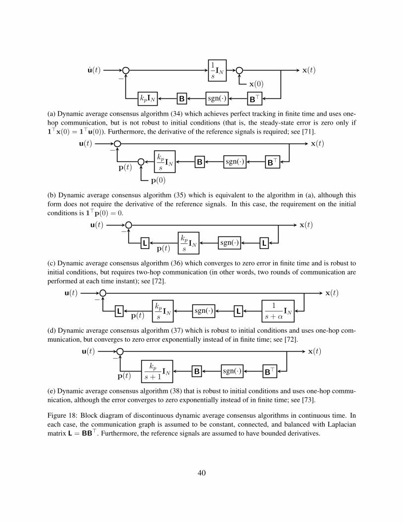
u(t)

kpIN B sgn(·) B>

1

sIN x(t)

x(0)−

(a) Dynamic average consensus algorithm (34) which achieves perfect tracking in finite time and uses one-hop communication, but is not robust to initial conditions (that is, the steady-state error is zero only if1>x(0) = 1>u(0)). Furthermore, the derivative of the reference signals is required; see [71].

u(t)

kps

IN B sgn(·) B>

x(t)

p(0)

−

p(t)

(b) Dynamic average consensus algorithm (35) which is equivalent to the algorithm in (a), although thisform does not require the derivative of the reference signals. In this case, the requirement on the initialconditions is 1>p(0) = 0.

u(t)

Lkps

IN sgn(·) L

x(t)

p(t)

−

(c) Dynamic average consensus algorithm (36) which converges to zero error in finite time and is robust toinitial conditions, but requires two-hop communication (in other words, two rounds of communication areperformed at each time instant); see [72].

u(t)

Lkps

IN sgn(·) L1

s+ αIN

x(t)

p(t)

−

(d) Dynamic average consensus algorithm (37) which is robust to initial conditions and uses one-hop com-munication, but converges to zero error exponentially instead of in finite time; see [72].

u(t)

kps+ 1

IN B sgn(·) B>

x(t)−

p(t)

(e) Dynamic average consensus algorithm (38) that is robust to initial conditions and uses one-hop commu-nication, although the error converges to zero exponentially instead of in finite time; see [73].

Figure 18: Block diagram of discontinuous dynamic average consensus algorithms in continuous time. Ineach case, the communication graph is assumed to be constant, connected, and balanced with Laplacianmatrix L = BB>. Furthermore, the reference signals are assumed to have bounded derivatives.

40

which moves the integrator before the Laplacian in the feedback loop. However, this dynamic aver-age consensus algorithm has two Laplacian blocks directly connected which means that it requirestwo-hop communication to implement. In other words, two sequential rounds of communicationare required at each time instant. In the time-domain, each agent must do the following (in order)at each time t: (1) communicate pi(t), (2) calculate xi(t), (3) communicate xi(t), and (4) updatepi(t) using the derivative pi(t). To only require one-hop communication, the dynamic averageconsensus algorithm in Figure 18d, given by

qi = −α qi + xi (37a)

pi = kp sgn( ∑j∈N iout

(qi − qj)), (37b)

xi = ui −∑j∈N iout

(pi − pj), pi(0), qi(0) ∈ R, i ∈ {1, . . . , N}, (37c)

places a strictly proper transfer function in the path between the Laplacian blocks. The extradynamics, however, cause the output to converge exponentially instead of in finite time [72].

Alternatively, under the given assumptions, a sliding mode-based dynamic average consensus al-gorithm with zero error tracking, which can be arbitrarily initialized is provided in [73] as

xi = ui − (xi − ui)− kp∑j∈N iout

sgn(xi − xj), xi(0) ∈ R, i ∈ {1, . . . , N},

or equivalently,

pi = −pi + kp∑j∈N iout

sgn(xi − xj), pi(0) ∈ R, (38a)

xi = ui − pi, i ∈ {1, . . . , N}. (38b)

However, this algorithm requires both the reference signals and their derivatives to be boundedwith known values γ1 and γ2: supτ∈[0,∞) ‖u(τ)‖ = γ1 < ∞ and supτ∈[0,∞) ‖u(τ)‖ = γ2 < ∞.These values are required to design the proper sliding mode gain kp.

The continuous-time finite-time algorithms described in this section exhibit a sliding mode behav-ior: in fact, they converge in finite time to the agreement manifold and then slide on it by switchingcontinuously at an infinite frequency between two system structures. This phenomenon is calledchattering. The reader may also recall that commutations at infinite frequency between two sub-systems is termed as the Zeno phenomenon in the literature of hybrid systems. The interestedreader can find an enlightening discussion on the relation between first-order sliding mode chat-tering and Zeno phenomenon in [74]. From a practical perspective, chattering is undesirable andleads to excessive control energy expenditure [75]. A common approach to eliminate chatteringis to smooth out the control discontinuity in a thin boundary layer around the switching surface.However, this approach leads to a tracking error that is propositional to the thickness of the bound-ary layer. Another approach to address is the use of higher-order sliding mode control, see [76] for

41

details. To the best of our knowledge, higher-order sliding mode control has not been used in thecontext of dynamic average consensus, although there exists results for other networked agreementproblems [77].

Conclusions

This article has provided an overview of the state of the art on the available distributed algorithmicsolutions to tackle the dynamic average consensus problem. We began by exploring several appli-cations of dynamic average consensus in cyber-physical systems, including distributed formationcontrol, state estimation, convex optimization, and optimal resource allocation. Using dynamicaverage consensus as a backbone, these advanced distributed algorithms enable groups of agentsto coordinate in order to solve complex problems. Starting from the static consensus problem,we then derived dynamic average consensus algorithms for various scenarios. We first introducedcontinuous-time algorithms along with simple techniques for analyzing them, using block dia-grams to provide intuition for the algorithmic structure. To reduce the communication bandwidth,we then showed how to choose the stepsizes to optimize the convergence rate when implementedin discrete time, along with how to accelerate the convergence rate by introducing extra dynamics.Finally, we showed how to use a priori information about the reference signals to design algorithmswith improved tracking performance.

We hope that the article helps the reader obtain an overview on the progress and intricacies of thistopic, and appreciate the design trade-offs faced when balancing desirable properties for large-scaleinterconnected systems such as convergence rate, steady-state error, robustness to initial condi-tions, internal stability, amount of memory required on each agent, and amount of communicationbetween neighboring agents. Given the importance of the ability to track the average of time-varying reference signals in network systems, we expect the number and breadth of applicationsfor dynamic average consensus algorithms to continue to increase in areas such as the smart grid,autonomous vehicles, and distributed robotics.

Many interesting questions and avenues for further research remain open. For instance, the emer-gence of opportunistic state-triggered ideas in the control and coordination of networked cyber-physical systems presents exciting opportunities for the development of novel solutions to the dy-namic average consensus problem. The underlying theme of this effort is to abandon the paradigmof periodic or continuous sampling/control in exchange for deliberate, opportunistic aperiodic sam-pling/control to improve efficiency. Beyond the brief incursion on this topic in “Dynamic AverageConsensus Algorithms with Continuous-Time Evolution and Discrete-Time Communication”, fur-ther research is needed in synthesizing triggering criteria for individual agents that prescribe wheninformation is to be shared with or acquired from neighbors, that lead to convergence guarantees,and that are amenable to the characterization of performance improvements over periodic discrete-time implementations. The use of event-triggering also opens up the way to employing otherinteresting forms of communication and computation among the agents when solving the dynamic

42

average consensus problem such as, for instance, the cloud. In cloud-based coordination, insteadof direct peer-to-peer communication, agents interact indirectly by opportunistically communicat-ing with the cloud to leave messages for other agents. These messages can contain informationabout their current estimates, future plans, or fallback strategies. The use of the cloud also opensthe possibility of network agents with limited capabilities taking advantage of high-performancecomputation capabilities to deal with complex processes. The time-varying nature of the signalsavailable at the individual agents in the dynamic average consensus problem raises many interest-ing challenges that need to be addressed to take advantage of this approach. Related to the focus ofthis effort on the communication aspects, the development of initialization-free dynamic averageconsensus algorithms over directed graphs is also another important line of research.

We believe that the interconnection of dynamic average consensus algorithms with other coordi-nation layers in network systems is a fertile area for both research and applications. Dynamicaverage consensus algorithms are a versatile tool in interconnected scenarios where it is necessaryto compute changing estimates of quantities that are employed by other coordination algorithms,and whose execution in turn affects the time-varying signals available to the individual agents.We have illustrated this in the “Applications of Dynamic Average Consensus in Network Sys-tems” section, where we described how in resource allocation problems, a group of distributedenergy resources can collectively estimate the mismatch between the aggregated power injectionand the desired load using dynamic average consensus. The computed mismatch in turn informsthe distributed energy resources in their decision making process seeking to determine the powerinjections that optimize their generation cost, which in turn changes the mismatch computed bythe dynamic average consensus algorithm. The fact that the time-varying nature of the signalsis driven by a dynamic process that itself uses the output of the dynamic average consensus algo-rithms opens the way for the use of many concepts germane to systems and control, including stableinterconnections, input-to-state stability, and passivity. Along these lines, we could also think ofself-tuning mechanisms embedded within dynamic average consensus algorithmic solutions thattune the algorithm execution based on the evolution of the time-varying signals.

Another interesting topic for future research is the privacy preservation of the signals availableto the agents in the dynamic average consensus problem. Protecting privacy and confidentialityof data is a critical issue in emerging distributed automated systems deployed in a variety of sce-narios, including power networks, smart transportation, the Internet of Things, and manufacturingsystems. In such scenarios, the ability of a network system to optimize its operation, fuse infor-mation, compute common estimates of unknown quantities, and agree on a common worldviewwhile protecting sensitive information is crucial. In this respect, the design of privacy-preservingdynamic average consensus algorithms is in its infancy. Interestingly, the dynamic nature of theproblem might offer advantages in this regard with respect to the static average consensus problem.For instance, in differential privacy, where the designer makes provably difficult for an adversaryto make inferences about individual records from published outputs, or even detect the presence ofan individual in the dataset, it is known that privacy guarantees weaken as more queries are madeto the same database. However, if the database is changing, this limitation no longer applies, andthis opens the way to studying how privacy guarantees change with the rate of variation of the

43

time-varying signals in the dynamic average consensus problem.

References

[1] R. Olfati-Saber, J. A. Fax, and R. M. Murray, “Consensus and cooperation in networked multi-agent systems,” Proceedings of the IEEE, vol. 95, no. 1, pp. 215–233, 2007.

[2] W. Ren and R. W. Beard, Distributed Consensus in Multi-Vehicle Cooperative Control, ser.Communications and Control Engineering. Springer, 2008.

[3] W. Ren and Y. Cao, Distributed Coordination of Multi-Agent Networks, ser. Communicationsand Control Engineering. New York: Springer, 2011.

[4] W. Ren, R. W. Beard, and E. M. Atkins, “Information consensus in multivehicle cooperativecontrol: Collective group behavior through local interaction,” IEEE Control Systems Maga-zine, vol. 27, no. 2, pp. 71–82, 2007.

[5] A. T. Kamal, J. A. Farrell, and A. K. Roy-Chowdhury, “Information weighted consensus fil-ters and their application in distributed camera networks,” IEEE Transactions on AutomaticControl, vol. 58, no. 12, pp. 3112–3125, 2013.

[6] D. Tian, J. Zhou, and Z. Sheng, “An adaptive fusion strategy for distributed information esti-mation over cooperative multi-agent networks,” IEEE Transactions on Information Theory.

[7] P. Yang, R. Freeman, and K. Lynch, “Optimal information propagation in sensor networks,” inProc. of the 2006 IEEE Int. Conf. on Robotics and Automation, 2006, pp. 3122–3127.

[8] K. M. Lynch, I. B. Schwartz, P. Yang, and R. A. Freeman, “Decentralized environmentalmodeling by mobile sensor networks,” IEEE Transactions on Robotics, vol. 24, no. 3, pp.710–724, 2008.

[9] P. Yang, R. A. Freeman, and K. M. Lynch, “Multi-agent coordination by decentralized estima-tion and control,” IEEE Transactions on Automatic Control, vol. 53, no. 11, pp. 2480–2496,2008.

[10] P. Yang, R. A. Freeman, G. J. Gordon, K. M. Lynch, S. S. Srinivasa, and R. Sukthankar,“Decentralized estimation and control of graph connectivity for mobile sensor networks,” Au-tomatica, vol. 46, no. 2, pp. 390–396, 2010.

[11] R. Aragues, J. Cortes, and C. Sagues, “Distributed consensus on robot networks for dy-namically merging feature-based maps,” IEEE Transactions on Robotics, vol. 28, no. 4, pp.840–854, 2012.

[12] S. Das and J. M. F. Moura, “Distributed Kalman filtering with dynamic observations consen-sus,” IEEE Transactions on Signal Processing, vol. 63, no. 17, pp. 4458–4473, Sep. 2015.

44

[13] F. Chen and W. Ren, “A connection between dynamic region-following formation control anddistributed average tracking,” IEEE Transactions on Cybernetics, 2018, to appear.

[14] J. A. Fax and R. M. Murray, “Information flow and cooperative control of vehicle forma-tions,” IEEE Transactions on Automatic Control, vol. 49, no. 9, pp. 1465–1476, 2004.

[15] W. Ren, “Multi-vehicle consensus with a time-varying reference state,” Systems and ControlLetters, vol. 56, no. 2, pp. 474–483, 2007.

[16] K. D. Listmann, M. V. Masalawala, and J. Adamy, “Consensus for formation control of non-holonomic mobile robots,” in IEEE Int. Conf. on Robotics and Automation, 2009, pp. 3886–3891.

[17] M. Porfiri, G. D. Roberson, and D. J. Stilwell, “Tracking and formation control of multipleautonomous agents: A two-level consensus approach,” Automatica, vol. 43, no. 8, pp. 1318–1328, 2007.

[18] S. Ghapani, S. Rahili, and W. Ren, “Distributed average tracking for second-order agentswith nonlinear dynamics,” in American Control Conference, 2016, pp. 4636–4641.

[19] S. S. Kia, J. Cortes, and S. Martınez, “Dynamic average consensus under limited controlauthority and privacy requirements,” International Journal on Robust and Nonlinear Control,vol. 25, no. 13, pp. 1941–1966, 2015.

[20] R. Olfati-Saber, “Distributed Kalman filter with embedded consensus filters,” in IEEE Conf.on Decision and Control, 2005, pp. 8179–8184.

[21] ——, “Kalman-consensus filter: Optimality, stability, and performance,” in IEEE Conf. onDecision and Control, 2009, pp. 7036–7042.

[22] W. Qi, P. Zhang, and Z. Deng, “Robust sequential covariance intersection fusion Kalmanfiltering over multi-agent sensor networks with measurement delays and uncertain noise vari-ances,” Acta Automatica Sinica, vol. 40, no. 11, pp. 2632–2642, 2014.

[23] G. Wang, N. Li, and Y. Zhang, “Diffusion distributed Kalman filter over sensor networkswithout exchanging raw measurements,” Signal Processing, vol. 132, pp. 1–7, 2017.

[24] R. Aragues, C. Sagues, and Y. Mezouar, “Feature-based map merging with dynamic consen-sus on information increments,” Autonomous Robots, vol. 38, no. 3, p. 243259, 2015.

[25] W. Ren and U. M. Al-Saggaf, “Distributed Kalman-Bucy filter with embedded dynamic av-eraging algorithm,” IEEE Systems Journal, vol. PP, no. 99, pp. 1–9, 2017.

[26] A. Nedic and A. Ozdaglar, “Distributed subgradient methods for multi-agent optimization,”IEEE Transactions on Automatic Control, vol. 54, no. 1, pp. 48–61, 2009.

45

[27] B. Johansson, M. Rabi, and M. Johansson, “A randomized incremental subgradient methodfor distributed optimization in networked systems,” SIAM Journal on Control and Optimiza-tion, vol. 20, no. 3, pp. 1157–1170, 2009.

[28] J. Wang and N. Elia, “A control perspective for centralized and distributed convex optimiza-tion,” in IEEE Conf. on Decision and Control, Orlando, Florida, 2011, pp. 3800–3805.

[29] M. Zhu and S. Martınez, “On distributed convex optimization under inequality and equalityconstraints,” IEEE Transactions on Automatic Control, vol. 57, no. 1, pp. 151–164, 2012.

[30] J. Lu and C. Y. Tang, “Zero-gradient-sum algorithms for distributed convex optimization: thecontinuous-time case,” IEEE Transactions on Automatic Control, vol. 57, no. 9, pp. 2348–2354, 2012.

[31] B. Gharesifard and J. Cortes, “Distributed continuous-time convex optimization on weight-balanced digraphs,” IEEE Transactions on Automatic Control, vol. 59, no. 3, pp. 781–786,2014.

[32] S. S. Kia, J. Cortes, and S. Martınez, “Distributed convex optimization via continuous-timecoordination algorithms with discrete-time communication,” Automatica, vol. 55, pp. 254–264, 2015.

[33] G. Qu and N. Li, “Accelerated distributed Nesterov gradient descent for convex and smoothfunctions,” in IEEE Conf. on Decision and Control, 2017, pp. 2260–2267.

[34] Y. Nesterov, Introductory lectures on convex optimization: a basic course. Springer Science& Business Media, 2014, vol. 87.

[35] R. Carli, G. Notarstefano, L. Schenato, and D. Varagnolo, “Analysis of Newton-Raphson con-sensus for multi-agent convex optimization under asynchronous and lossy communication,” inIEEE Conf. on Decision and Control, Osaka, Japan, Dec. 2015, pp. 418–424.

[36] J. Xu, S. Zhu, Y. C. Soh, and L. Xie, “Augmented distributed gradient methods for multi-agent optimization under uncoordinated constant stepsizes,” in IEEE Conf. on Decision andControl, Osaka, Japan, 2015.

[37] D. Varagnolo, F. Zanella, P. G. A. Cenedese, and L. Schenato, “Newton-Raphson consensusfor distributed convex optimization,” IEEE Transactions on Automatic Control, vol. 61, no. 4,pp. 994–1009, 2016.

[38] P. D. Lorenzo and G. Scutari, “NEXT: In-network nonconvex optimization,” IEEE Transac-tions on Signal and Information Processing over Networks, vol. 2, no. 2, pp. 120–136, 2016.

[39] A. Nedic, A. Olshevsky, and W. Shi, “Achieving geometric convergence for distributed opti-mization over time-varying graphs,” IEEE Transactions on Signal and Information Processingover Networks, vol. 27, no. 4, pp. 2597–2633, 2017.

46

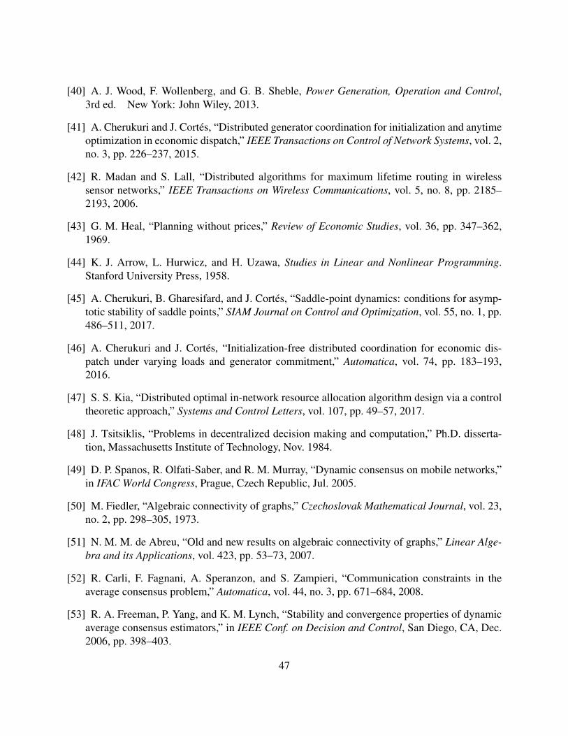
[40] A. J. Wood, F. Wollenberg, and G. B. Sheble, Power Generation, Operation and Control,3rd ed. New York: John Wiley, 2013.

[41] A. Cherukuri and J. Cortes, “Distributed generator coordination for initialization and anytimeoptimization in economic dispatch,” IEEE Transactions on Control of Network Systems, vol. 2,no. 3, pp. 226–237, 2015.

[42] R. Madan and S. Lall, “Distributed algorithms for maximum lifetime routing in wirelesssensor networks,” IEEE Transactions on Wireless Communications, vol. 5, no. 8, pp. 2185–2193, 2006.

[43] G. M. Heal, “Planning without prices,” Review of Economic Studies, vol. 36, pp. 347–362,1969.

[44] K. J. Arrow, L. Hurwicz, and H. Uzawa, Studies in Linear and Nonlinear Programming.Stanford University Press, 1958.

[45] A. Cherukuri, B. Gharesifard, and J. Cortes, “Saddle-point dynamics: conditions for asymp-totic stability of saddle points,” SIAM Journal on Control and Optimization, vol. 55, no. 1, pp.486–511, 2017.

[46] A. Cherukuri and J. Cortes, “Initialization-free distributed coordination for economic dis-patch under varying loads and generator commitment,” Automatica, vol. 74, pp. 183–193,2016.

[47] S. S. Kia, “Distributed optimal in-network resource allocation algorithm design via a controltheoretic approach,” Systems and Control Letters, vol. 107, pp. 49–57, 2017.

[48] J. Tsitsiklis, “Problems in decentralized decision making and computation,” Ph.D. disserta-tion, Massachusetts Institute of Technology, Nov. 1984.

[49] D. P. Spanos, R. Olfati-Saber, and R. M. Murray, “Dynamic consensus on mobile networks,”in IFAC World Congress, Prague, Czech Republic, Jul. 2005.

[50] M. Fiedler, “Algebraic connectivity of graphs,” Czechoslovak Mathematical Journal, vol. 23,no. 2, pp. 298–305, 1973.

[51] N. M. M. de Abreu, “Old and new results on algebraic connectivity of graphs,” Linear Alge-bra and its Applications, vol. 423, pp. 53–73, 2007.

[52] R. Carli, F. Fagnani, A. Speranzon, and S. Zampieri, “Communication constraints in theaverage consensus problem,” Automatica, vol. 44, no. 3, pp. 671–684, 2008.

[53] R. A. Freeman, P. Yang, and K. M. Lynch, “Stability and convergence properties of dynamicaverage consensus estimators,” in IEEE Conf. on Decision and Control, San Diego, CA, Dec.2006, pp. 398–403.

47

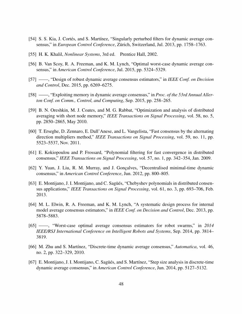
[54] S. S. Kia, J. Cortes, and S. Martınez, “Singularly perturbed filters for dynamic average con-sensus,” in European Control Conference, Zurich, Switzerland, Jul. 2013, pp. 1758–1763.

[55] H. K. Khalil, Nonlinear Systems, 3rd ed. Prentice Hall, 2002.

[56] B. Van Scoy, R. A. Freeman, and K. M. Lynch, “Optimal worst-case dynamic average con-sensus,” in American Control Conference, Jul. 2015, pp. 5324–5329.

[57] ——, “Design of robust dynamic average consensus estimators,” in IEEE Conf. on Decisionand Control, Dec. 2015, pp. 6269–6275.

[58] ——, “Exploiting memory in dynamic average consensus,” in Proc. of the 53rd Annual Aller-ton Conf. on Comm., Control, and Computing, Sep. 2015, pp. 258–265.

[59] B. N. Oreshkin, M. J. Coates, and M. G. Rabbat, “Optimization and analysis of distributedaveraging with short node memory,” IEEE Transactions on Signal Processing, vol. 58, no. 5,pp. 2850–2865, May 2010.

[60] T. Erseghe, D. Zennaro, E. Dall’Anese, and L. Vangelista, “Fast consensus by the alternatingdirection multipliers method,” IEEE Transactions on Signal Processing, vol. 59, no. 11, pp.5523–5537, Nov. 2011.

[61] E. Kokiopoulou and P. Frossard, “Polynomial filtering for fast convergence in distributedconsensus,” IEEE Transactions on Signal Processing, vol. 57, no. 1, pp. 342–354, Jan. 2009.

[62] Y. Yuan, J. Liu, R. M. Murray, and J. Goncalves, “Decentralised minimal-time dynamicconsensus,” in American Control Conference, Jun. 2012, pp. 800–805.

[63] E. Montijano, J. I. Montijano, and C. Sagues, “Chebyshev polynomials in distributed consen-sus applications,” IEEE Transactions on Signal Processing, vol. 61, no. 3, pp. 693–706, Feb.2013.

[64] M. L. Elwin, R. A. Freeman, and K. M. Lynch, “A systematic design process for internalmodel average consensus estimators,” in IEEE Conf. on Decision and Control, Dec. 2013, pp.5878–5883.

[65] ——, “Worst-case optimal average consensus estimators for robot swarms,” in 2014IEEE/RSJ International Conference on Intelligent Robots and Systems, Sep. 2014, pp. 3814–3819.

[66] M. Zhu and S. Martınez, “Discrete-time dynamic average consensus,” Automatica, vol. 46,no. 2, pp. 322–329, 2010.

[67] E. Montijano, J. I. Montijano, C. Sagues, and S. Martınez, “Step size analysis in discrete-timedynamic average consensus,” in American Control Conference, Jun. 2014, pp. 5127–5132.

48

[68] H. Bai, R. A. Freeman, and K. M. Lynch, “Robust dynamic average consensus of time-varying inputs,” in IEEE Conf. on Decision and Control, Atlanta, GA, Dec. 2010, pp. 3104–3109.

[69] H. Bai, “Adaptive motion coordination with an unknown reference velocity,” in AmericanControl Conference, Jul. 2015, pp. 5581–5586.

[70] B. V. Scoy, R. A. Freeman, and K. M. Lynch, “Feedforward estimators for the distributedaverage tracking of bandlimited signals in discrete time with switching graph topology,” inIEEE Conf. on Decision and Control, Dec. 2016, pp. 4284–4289.

[71] F. Chen, Y. Cao, and W. Ren, “Distributed average tracking of multiple time-varying ref-erence signals with bounded derivatives,” IEEE Transactions on Automatic Control, vol. 57,no. 12, pp. 3169–3174, 2012.

[72] J. George, R. A. Freeman, and K. M. Lynch, “Robust dynamic average consensus algorithmfor signals with bounded derivatives,” in American Control Conference, May 2017, pp. 352–357.

[73] S. Rahili and W. Ren, “Heterogeneous distributed average tracking using nonsmooth algo-rithms,” in American Control Conference, Jul. 2017, pp. 691–696.

[74] L. Yu, J. P. Barbot, D. Benmerzouk, D. Boutat, T. Floquet, and G. Zheng,Discussion about Sliding Mode Algorithms, Zeno Phenomena and Observability. Berlin,Heidelberg: Springer Berlin Heidelberg, 2012, pp. 199–219. [Online]. Available:https://doi.org/10.1007/978-3-642-22164-4 7

[75] J.-J. E. Slotine and W. Li, Applied Nonlinear Control. Prentice Hall, 1991.

[76] L. Fridman and A. Levant, Higher order sliding modes. New York: CRC Press, 2002, pp.53–101.

[77] E. G. Rojo-Rodriguez, E. J. Ollervides, J. G. Rodriguez, E. S. Espinoza, P. Zambrano-Robledo, and O. Garcia, “Implementation of a super twisting controller for distributed forma-tion flight of multi-agent systems based on consensus algorithms,” in International Conferenceon Unmanned Aircraft Systems, Miami, FL, 2017.

49

Sidebar: Article SummaryThis article deals with the dynamic average consensus problem and the distributed coordinationalgorithms available to solve it. Such problem arises in scenarios with multiple agents, where eachone has access to a time-varying signal of interest (for example, a robot sensor sampling the posi-tion of a mobile target of interest or a distributed energy resource taking a sequence of frequencymeasurements in a microgrid). The dynamic average consensus problem consists of having themulti-agent network collectively compute the average of the set of time-varying signals. Rea-sons for pursuing this objective are numerous, and include data fusion, refinement of uncertaintyguarantees, and computation of higher-accuracy estimates, all enabling local decision making withnetwork-wide aggregated information. Solving this problem is challenging because the local inter-actions among agents only involve partial information and the quantity that the network seeks tocompute is changing as the agents run their routines. The article provides a tutorial introduction todistributed methods that solve the dynamic average consensus problems, paying special attentionto the role of network connectivity, incorporating information about the nature of the time-varyingsignals, the performance trade-offs regarding convergence rate, steady-state error and memory andcommunication requirements, and algorithm robustness against initialization errors.

50

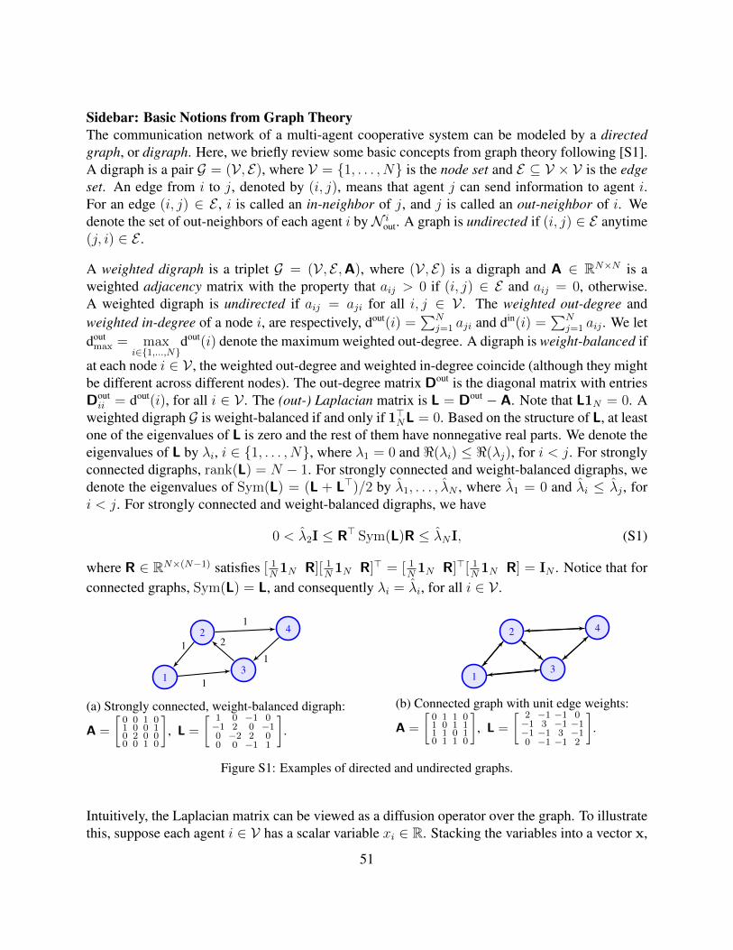
Sidebar: Basic Notions from Graph TheoryThe communication network of a multi-agent cooperative system can be modeled by a directedgraph, or digraph. Here, we briefly review some basic concepts from graph theory following [S1].A digraph is a pair G = (V , E), where V = {1, . . . , N} is the node set and E ⊆ V × V is the edgeset. An edge from i to j, denoted by (i, j), means that agent j can send information to agent i.For an edge (i, j) ∈ E , i is called an in-neighbor of j, and j is called an out-neighbor of i. Wedenote the set of out-neighbors of each agent i byN i

out. A graph is undirected if (i, j) ∈ E anytime(j, i) ∈ E .

A weighted digraph is a triplet G = (V , E ,A), where (V , E) is a digraph and A ∈ RN×N is aweighted adjacency matrix with the property that aij > 0 if (i, j) ∈ E and aij = 0, otherwise.A weighted digraph is undirected if aij = aji for all i, j ∈ V . The weighted out-degree andweighted in-degree of a node i, are respectively, dout(i) =

∑Nj=1 aji and din(i) =

∑Nj=1 aij . We let

doutmax = max

i∈{1,...,N}dout(i) denote the maximum weighted out-degree. A digraph is weight-balanced if

at each node i ∈ V , the weighted out-degree and weighted in-degree coincide (although they mightbe different across different nodes). The out-degree matrix Dout is the diagonal matrix with entriesDoutii = dout(i), for all i ∈ V . The (out-) Laplacian matrix is L = Dout − A. Note that L1N = 0. A

weighted digraph G is weight-balanced if and only if 1>NL = 0. Based on the structure of L, at leastone of the eigenvalues of L is zero and the rest of them have nonnegative real parts. We denote theeigenvalues of L by λi, i ∈ {1, . . . , N}, where λ1 = 0 and <(λi) ≤ <(λj), for i < j. For stronglyconnected digraphs, rank(L) = N − 1. For strongly connected and weight-balanced digraphs, wedenote the eigenvalues of Sym(L) = (L + L>)/2 by λ1, . . . , λN , where λ1 = 0 and λi ≤ λj , fori < j. For strongly connected and weight-balanced digraphs, we have

0 < λ2I ≤ R> Sym(L)R ≤ λNI, (S1)

where R ∈ RN×(N−1) satisfies [ 1N

1N R][ 1N

1N R]> = [ 1N

1N R]>[ 1N

1N R] = IN . Notice that forconnected graphs, Sym(L) = L, and consequently λi = λi, for all i ∈ V .

1

2

3

4

1

1

2

1

1

(a) Strongly connected, weight-balanced digraph:

A =

[0 0 1 01 0 0 10 2 0 00 0 1 0

], L =

[ 1 0 −1 0−1 2 0 −10 −2 2 00 0 −1 1

].

1

2

3

4

(b) Connected graph with unit edge weights:

A =

[0 1 1 01 0 1 11 1 0 10 1 1 0

], L =

[ 2 −1 −1 0−1 3 −1 −1−1 −1 3 −10 −1 −1 2

].

Figure S1: Examples of directed and undirected graphs.

Intuitively, the Laplacian matrix can be viewed as a diffusion operator over the graph. To illustratethis, suppose each agent i ∈ V has a scalar variable xi ∈ R. Stacking the variables into a vector x,

51

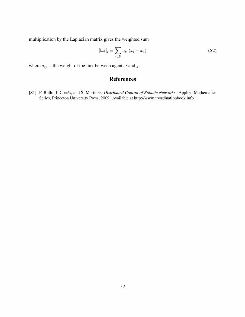
multiplication by the Laplacian matrix gives the weighted sum

[Lx]i =∑j∈V

aij (xi − xj) (S2)

where aij is the weight of the link between agents i and j.

References

[S1] F. Bullo, J. Cortes, and S. Martınez, Distributed Control of Robotic Networks. Applied MathematicsSeries, Princeton University Press, 2009. Available at http://www.coordinationbook.info.

52

Sidebar: Input-to-State Stability of LTI SystemsFor a linear time-invariant system

x = Ax + Bu, x ∈ Rn, u ∈ Rm, (S3)

we can write the solution for t ∈ R≥0 as

x(t) = eA t x(0) +

∫ t

0

eA(t−τ) B u(τ)dτ. (S4)

For a Hurwitz matrix A, by using the bound

‖eA t‖ ≤ κ e−λ t, t ∈ R≥0, (S5)

for some κ, λ ∈ R>0, we can establish an upper bound on the norm of the trajectories of (S4) asfollows

‖x(t)‖ ≤ κ e−λ t ‖x(0)‖+

∫ t

0

κ e−λ (t−τ)‖B‖ ‖u(τ)‖dτ,

≤ κ e−λ t ‖x(0)‖+κ ‖B‖λ

sup0≤τ≤t

‖u(τ)‖, ∀t ∈ R≥0. (S6)

The bound here shows that the zero-input response decays to zero exponentially fast, while thezero-state response is bounded for every bounded input, indicating an input-to-state stability (ISS)behavior. It is worth noticing that the ultimate bound on the system state is proportional to thebound on the input.

Next, we comment on how to compute the parameters κ, λ ∈ R>0 in (S5). Recall that [S20, Fact11.15.5] for any matrix A ∈ Rn×n, we can write

‖eA t‖ ≤ eλmax(Sym(A)) t. ∀ t ∈ R≥0 (S7)

where Sym(A) = 12(A+A>). Therefore, for a Hurwitz matrix A whose Sym(A) is also Hurwitz,

the exponential bound parameters can be set to

λ = −λmax(Sym(A)), κ = 1. (S8)

A tighter exponential bound of

λ = λ?, κ =√σmax(P?)/σmin(P?), (S9)

can also be obtained for any Hurwitz, according to [S21, Proposition 5.5.33], from the convexlinear matrix inequality optimization problem

(λ?,P?) = argminλ s.t. (S10a)

PA + A>P ≤ −2λP, P > 0, λ > 0. (S10b)

53

Similarly, the state of the discrete-time linear time-invariant system

xk+1 = Axk + Buk, xk ∈ Rn, uk ∈ Rm (S11)

with initial condition x0 ∈ Rn satisfies the bound

‖xk‖ ≤

√σmax(P)

σmin(P)

(ρk‖x0‖+

1− ρk

1− ρ‖B‖ sup

0≤j<k‖uj‖

)(S12)

where P ∈ Rn×n and ρ ∈ R satisfy

A>PA− ρ2 P ≤ 0, P > 0, ρ ≥ 0. (S13)

References

[S20] D. S. Bernstein, Matrix Mathematics: Theory, Facts, and Formulas with Application to Linear SystemTheory. Springer-Verlag Berlin Heidelberg, 2005.

[S21] D. Hinrichsen and A. J. Pritchard, Mathematical Systems Theory I: Modeling, State Space Analysis,Stability and Robustness. Princeton University Press, 2005.

54

Sidebar: Further Reading

Numerous works have studied the robustness of dynamic average consensus algorithms against avariety of disturbances and sources of error present in practical scenarios. These include fixed com-munication delays [S2], additive input disturbances [S7], time-varying communication graphs [S17],and driving command saturation [19]. Variations of the dynamic average consensus problems ex-plore scenarios where the algorithm design depends on the specific agent dynamics [S4, S3, 73]or incorporates different agent roles, such as in leader-follower networks of mobile agents [S5, S6,S8].

When dealing with directed agent interactions, a common assumption in solving the average con-sensus problem is that the communication graph is weight-balanced, which is equivalent to thegraph consensus matrix W := I − L being doubly stochastic. In [S9], it is shown in fact thatcalculating an average over a network requires either explicit or implicit use of either (1) the out-degree of each agent, (2) global node identifiers, (3) randomization, or (4) asynchronous updateswith specific properties. In particular, the balanced assumption is necessary for scalable, deter-ministic, synchronous algorithms. In general, agents may not have access to their out-degree (forexample, agents which use local broadcast communication). If each agent knows its out-degree,however, then distributed algorithms may be used to generate weight-balanced and doubly stochas-tic digraphs [S10, S11]. Another approach is to explicitly use the out-degree in the algorithm byhaving agents share their out-weights and use them to adjust for the imbalances in the graph; thisapproach is referred to as the push-sum protocol and has been applied to the static average con-sensus problem (see [S13, S14, S15, S16]). Both of these approaches of dealing with unbalancedgraphs require each agent to know its out-degree.

Furthermore, when communication links are time-varying, these approaches only work if thetime-varying graph remains weight-balanced, see [19, S28]. If communication failures causedby limited communication ranges or external events such as obstacle blocking destroy the weight-balanced character of the graph, it is still possible to solve the dynamic average consensus problemif the expected graph is balanced [S17]. Another set of works have explored the question of how tooptimize the graph topology to endow consensus algorithms with better properties. These includedesigning the network topology in the presence of random link failures [S18] and optimizing theedge weights for fast consensus [S19, 7].

References

[S2] H. Moradian and S. S. Kia, “Dynamic average consensus in the presence of communication delay overdirected graph topologies,” in American Control Conference, pp. 4663–4668, 2017.

[S3] S. Ghapania and W. Ren and F. Chen and Y. Song, “Distributed average tracking for double-integratormulti-agent systems with reduced requirement on velocity measurements,” Automatica, vol. 81, no. 7,pp. 1–7, 2017.

55

[S4] F. Chen and G. Feng and L. Liu and W. Ren, “Distributed Average Tracking of Networked Euler-Lagrange Systems,” in IEEE Transactions on Automatic Control, vol. 60, no. 2, pp. 547–552, 2015.

[S5] W. Ren, “Multi-vehicle consensus with a time-varying reference state,” Systems and Control Letters,vol. 52, no. 2, pp. 474–483, 2007.

[S6] G. Shi and Y. Hong and K. H. Johansson, “Connectivity and set tracking of multi-agent systems guidedby multiple moving leaders,” IEEE Transactions on Automatic Control, vol. 57, no. 3, pp. 663–676,2012.

[S7] G. Shi and K. H. Johansson, “Robust consensus for continuous-time multi-agent dynamics,” SIAMJournal on Control and Optimization, vol. 51, no. 5, pp. 3673–3691, 2013.

[S8] Z. Meng, D. V. Dimarogonas and K. H. Johansson, “Leader-follower coordinated tracking of multipleheterogeneous Lagrange systems using continuous control,” IEEE Transactions on Robotics, vol. 30,no. 3, pp. 739–745, 2014.

[S9] J. M. Hendrickx and J. N. Tsitsiklis, “Fundamental limitations for anonymous distributed systems withbroadcast communications,” in Allerton Conference on Communication, Control, and Computing, pp.9–16, 2015.

[S10] B. Gharesifard and J. Cortes, “Distributed strategies for generating weight-balanced and doublystochastic digraphs,” European Journal of Control, vol. 18, no. 6, pp. 539–557, 2012.

[S11] A. Rikos, T. Charalambous and C. N. Hadjicostis, “Distributed weight balancing over digraphs,”IEEE Transactions on Control of Network Systems, vol. 1, no. 2, pp. 190–201, 2014.

[S12] D. Kempe, A. Dobra, and J. Gehrke, “Gossip-based computation of aggregate information,” in IEEESymposium on Foundations of Computer Science, (Washington, DC), pp. 482-491, 2003.

[S13] F. Benezit, V. Blondel, P. Thiran, J. Tsitsiklis, and M. Vetterli, “Weighted gossip: Distributed aver-aging using non-doubly stochastic matrices,” in IEEE International Symposium on Information TheoryProceedings, pp. 1753-1757, 2010.

[S14] A. D. Domınguez-Garcıa and C. N. Hadjicostis, “Distributed matrix scaling and application to aver-age consensus in directed graphs,” IEEE Transactions on Automatic Control, vol. 58, no. 3, pp. 667–681, 2013.

[S15] A. Nedic and A. Olshevsky, “Distributed optimization over time-varying directed graphs,” IEEETransactions on Automatic Control, vol. 60, no. 3, pp. 601–615, 2015.

[S16] P. Rezaienia, B. Gharesifard, T. Linder, and B. Touri, “Push-sum on random graphs,” https://arxiv.org/abs/1708.00915, 2017.

[S17] B. Van Scoy, R. A. Freeman, and K. M. Lynch, “Asymptotic mean ergodicity of average consensusestimators,” in American Control Conference, 2014, pp. 4696–4701.

[S18] S. Kar and J.M.F. Moura, “Sensor Networks With Random Links: Topology Design for DistributedConsensus,” in IEEE Transactions on Signal Processing, vol. 56, no. 7, pp. 3315–3326, 2008.

56

[S19] L. Xiao and S. Boyd, “Fast linear iterations for distributed averaging,” in IEEE Conf. on Decisionand Control, 2003, pp. 4997–5002.

57

Sidebar: Euler Discretizations of Continuous-Time Dynamic Average Consensus AlgorithmsThe continuous-time algorithms described in the article can also give rise to discrete-time strate-gies. Here we describe how to discretize them so that they are implementable over wireless com-munication channels. This can be done by using the (forward) Euler discretization of the deriva-tives,

x(t) ≈ x(k + 1)− x(k)

δ,

where δ ∈ R>0 is the stepsize. To illustrate the discussion, we develop this approach for thealgorithm (25) over a connected graph topology. The discussion below can also be extended toinclude iterative forms of the other continuous-time algorithms studied in the paper. Using theEuler discretization in the algorithm (25) leads to

vi(k + 1) = vi(k) + δαβ∑N

j=1aij(x

i(k)−xj(k)), (S14a)

xi(k + 1) = xi(k) + ∆ui(k)− δα(xi(k)− ui(k))− δβ∑N

j=1aij(x

i(k)− xj(k))− δvi(k),

(S14b)

where ∆ui(k) = ui(k + 1) − ui(k). To implement this iterative form at each timestep k we needto have access to the future value of the reference input at timestep k + 1. Such a requirement isnot practical when the reference input is sampled from a physical process or is a result of anotheron-line algorithm. We could circumvent this requirement using a backward Euler discretization,but the resulting algorithm tracks the reference dynamic average with one-step delay. A practicalsolution which avoids requiring the future values of the reference input is obtained by introducingan intermediate variable zi(k) = xi(k) − ui(k) and representing the iterative algorithm (S14) inthe form

vi(k + 1) = vi(k) + δαβ∑N

j=1aij(x

i(k)−xj(k)), (S15a)

zi(k + 1) = zi(k)− δαzi(k)− δβ∑N

j=1aij(x

i(k)− xj(k))− δvi(k), (S15b)

xi(k) = zi(k) + ui(k), (S15c)

for i ∈ {1, . . . , N}. Algorithm (S15) is then implementable without the use of future inputs.

The question then is to characterize the adequate stepsizes that guarantee that the convergenceproperties of the continuous-time algorithm are retained by its discrete implementation. Intuitively,the smaller the stepsize, the better for this purpose. However, this also requires more communica-tion. To ascertain this issue, the following result is particularly useful.

Lemma 3 (Admissible stepsize for Euler discretized form of LTI systems and a boundon their trajectories). Consider

x = Ax + Bu, t ∈ R≥0,

58

and its Euler discretized iterative form

x(k + 1) = (I + δA) x(k) + δB u(k), k ∈ Z≥0, (S16)

where x ∈ Rn and u ∈ Rm are, respectively, state and input vectors, and δ ∈ R>0 is the dis-cretization stepsize. Let the system matrix A = [aij] ∈ Rn×n be a Hurwitz matrix with eigenvalues{µi}ni=1, and the difference of input signal be bounded, ‖∆u‖ < ρ < ∞. Then, for any δ ∈ (0, d)where

d = min{− 2

Re(µi)

|µi|2}ni=1

(S17)

the eigenvalues of (I + δA) are all located inside the until circle in complex plane. Moreover,starting from any x(0) ∈ Rn, the trajectories of (S16) satisfy

limk→∞‖x(k + 1)‖ ≤ κ ρ ‖B‖

1− ω, (S18)

where ω ∈ (0, 1), and κ ∈ R > 0 such that ‖I + δA‖k ≤ κωk.

The bounds ω ∈ (0, 1) and κ ∈ R>0 in ‖I + δA‖k ≤ κωk when all the eigenvalues of I + δA arelocated in the unit circle of the complex plane can be obtained from the following LMI optimizationproblem (see [S22, Theorem 23.3] for details)

(ω, κ,Q) = argminω2, subject to (S19)1

κI ≤ Q ≤ I, 0 < ω2 < 1, κ > 1,

(I + δA)>Q (I + δA)−Q ≤ −(1− ω2) I.

Building on Lemma 3, the next result characterizes the admissible discretization stepsize for thealgorithm (S15) and its ultimate tracking behavior.

Theorem 6 (Convergence of (S15) over connected graphs [19]). Let G be a connected,undirected graph. Assume that the differences of the inputs of the network satisfy maxk∈Z≥0

‖(I−1N

1N1>N) ∆u(k)‖ = γ < ∞. Then, for any α, β > 0, the algorithm (S15) over G initialized atzi(0) ∈ R and vi(0) ∈ R such that

∑Ni=1 v

i(0) = 0 has bounded trajectories that satisfy

limk→∞

∣∣xi(k)− uavg(k)∣∣ ≤ δ κ γ

1− ω, i ∈ {1, . . . , N} (S20)

provided δ ∈ (0,min{α−1, 2 β−1(λN)−1}). Here, λN is the largest eigenvalue of the Laplacian,and ω ∈ (0, 1) and κ ∈ R>0 satisfy ‖I− δ β R>LR‖k ≤ κωk, k ∈ Z≥0.

Note that the characterization of the stepsize requires knowledge of the largest eigenvalue λNof the Laplacian. Since such knowledge is not readily available to the network unless dedicateddistributed algorithms are introduced to compute it, [19] provides the sufficient characterizationδ ∈ (0,min{α−1, β−1(dmax

out )−1}) along with the ultimate tracking bound

limk→∞

∣∣xi(k)− uavg(k)∣∣ ≤ δγ

β λ2

, i ∈ {1, . . . , N}.

59

References

[S22] W. J. Rugh, Linear Systems Theory. Prentice Hall: Englewood Cliffs, NJ, 1993.

60

Sidebar: Dynamic Average Consensus Algorithms with Continuous-Time Evolution andDiscrete-Time Communication

We discuss here an alternative to the discretization route explained in “Euler Discretizations ofContinuous-Time Dynamic Average Consensus Algorithms” to produce implementable strategiesfrom the continuous-time algorithms described in the paper. This approach is based on the ob-servation that, when implementing the algorithms over digital platforms, computation can still bereasonably approximated by continuous-time evolution (given the every growing computing capa-bilities of modern embedded processors and computers) whereas communication is a process thatstill requires proper acknowledgment of its discrete-time nature. Our basic idea is to opportunis-tically trigger, based on the network state, the times for information sharing among agents to takeplace, and to allow individual agents to determine these autonomously. This has the potential toresult in more efficient algorithm implementations as performing communication usually requiresmore energy than computation [S23]. In addition, the use of fixed communication stepsizes canlead to a wasteful use of the network resources because of the need to select it taking into accountworst-case scenarios. These observations are aligned with the ongoing research activity [S24, S25]on event-triggered control and aperiodic sampling for controlled dynamical systems that seeks totrade computation and decision making for less communication, sensing or actuator effort whilestill guaranteeing a desired level of performance. The surveys [S26, S27] describe how these ideascan be employed to design event-triggered communication laws for static average consensus.

Motivated by these observations, [S28] investigates a discrete-time communication implementa-tion of the continuous-time algorithm (25) for dynamic average consensus. Under this strategy thealgorithm becomes

vi = αβ∑N

j=1aij(x

i − xj), (S21a)

xi = ui−α(xi − ui)−β∑N

j=1aij(x

i−xj)−vi, (S21b)

for each i ∈ {1, . . . , N}, where xi(t) = xi(tik) for t ∈ [tik, tik+1), with {tik} ⊂ R≥0 denoting the

sequence of times at which agent i communicates with its in-neighbors. The basic idea is thatagents share their information with neighbors when the uncertainty in the outdated information issuch that the monotonic convergent behavior of the overall network can no longer be guaranteed.The design of such triggers is challenging because of the following requirements: (a) triggers needto be distributed, so that agents can check them with the information available to them from theirout-neighbors, (b) they must guarantee the absence of Zeno behavior (the undesirable situationwhere an infinite number of communication rounds are triggered in a finite amount of time), and (c)they have to ensure the network achieves dynamic average consensus even though agents operatewith outdated information while inputs are changing with time.

Consider the following event-triggered communication law [S28]: each agent is to communicate

61

with its in-neighbors at times {tik}k∈N ⊂ R≥0, starting at ti1 = 0, determined by

tik+1 =argmax{t ∈ [tik,∞) | |xi(tik)− xi(t)| ≤ εi}. (S22)

Here, εi ∈ R>0 is a constant value which each agent chooses locally to control its inter-event timesand avoid Zeno behavior. Specifically, the inter-execution times of each agent i ∈ {1, . . . , N}employing (S22) are lower bounded by

τ i =1

αln(

1 +αεici

), (S23)

where ci and η are positive real numbers that depend on the initial conditions and network param-eters (we omit here for simplicity their specific form, but the interested reader is referred to [S28]for explicit expressions). The lower bound (S23) shows that for a positive nonzero εi, the inter-execution times are bounded away from zero and we have the guarantees that for networks withfinite number of agents the implementation of the algorithm (S21) with the communication triggerlaw (S22) is Zeno free. The following result formally describes the convergence behavior of thealgorithm (S21) under (S22) When the interaction topology is modeled by a strongly connectedand weight-balanced digraph.

Theorem 7 (Convergence of (S21) over strongly connected and weight-balanced digraphwith asynchronous distributed event-triggered communication [S28]). Let G be a strongly con-nected and weight-balanced digraph. Assume the reference signals satisfy supt∈[0,∞) |ui(t)| =κi < ∞, for i ∈ {1, . . . , N}, and supt∈[0,∞) ‖ΠN u(t)‖ = γ < ∞. For any α, β ∈ R>0, thealgorithm (S21) over G starting from xi(0) ∈ R and vi(0) ∈ R with

∑Ni=1 v

i(0) = 0, where eachagent i ∈ {1, . . . , N} communicates with its neighbors at times {tik}k∈N ⊂ R≥0, starting at ti1 = 0,determined by (S22) with ε ∈ RN

>0, satisfies

lim supt→∞

∣∣∣xi(t)−uavg(t)∣∣∣≤ γ+β‖L‖ ‖ε‖

βλ2

, (S24)

for i ∈ {1, . . . , N} with an exponential rate of convergence of min{α, βλ2}. Furthermore, theinter-execution times of agent i ∈ {1, . . . , N} are lower bounded by (S23).

The expected trade-off between the desire for longer inter-event time and the adverse effect on sys-tems convergence and performance is captured in (S23) and (S24). The lower bound τ i in (S23)on the inter-event times allows a designer to compute bounds on the maximum number of com-munication rounds (and associated energy spent) by each agent i ∈ {1, . . . , N} (and hence thenetwork) during any given time interval. It is interesting to analyze how this lower bound dependson the various problem ingredients: τ i is an increasing function of εi and a decreasing functionof α and ci. Through the latter variable, the bound also depends on the graph topology and thedesign parameter β. Given the definition of ci, we can deduce that the faster an input of an agent ischanging (larger κi) or the farther the agent initially starts from the average of the inputs, the more

62

often that agent would need to trigger communication. The connection between the network per-formance and the communication overhead can also be observed here. Increasing β or decreasingεi to improve the ultimate tracking error bound (S24) results in smaller inter-event times. Giventhat the rate of convergence of (S21) under (S22) is min{α, βλ2}, decreasing α to increase theinter-event times slows down the convergence.

When the interaction topology is a connected graph, the properties of the Laplacian allow us toidentify an alternative event-triggered communication law which, compared to (S22), has a longerinter-event time but similar dynamic average tracking performance. Now, consider the sequenceof communication times {tik}k∈N determined by

tik+1 = argmax{t ∈ [tik,∞) | |xi(t)− xi(t)|2 ≤ (S25)

1

4diout

N∑j=1

aij(t)|xi(t)− xj(t)|2 +1

4diout

ε2i },

Compared to (S22), the extra term 14diout

∑Nj=1 aij(t)|xi(t)−xj(t)|2 in the communication law (S25)

allows agents to have longer inter-event times. Formally, the inter-execution times of agent i ∈{1, . . . , N} implementing (S25) are lower bounded by

τ i =1

αln(

1 +αεi

2ci√

diout

), (S26)

for positive constants ci, see [S28] for explicit expressions. Numerical examples in [S28] showthat the implementation of (S25) for connected graphs results in inter-event times longer than theones of the event-triggered law (S22). Figure S2 shows one of those examples. Similar results canalso be derived for time-varying, jointly connected graphs, see [S28] for a complete exposition.

References

[S23] H. Karl and A. Willig, Protocols and Architectures for Wireless Sensor Networks. John Wiley: NewYork, 2005.

[S24] W. P. M. H. Heemels, K. H. Johansson, and P. Tabuada, “An introduction to event-triggered andself-triggered control,” in IEEE Conf. on Decision and Control, pp. 3270–3285, Maui, HI, 2012.

[S25] L. Hetel, C. Fiter, H. Omran, A. Seuret, E. Fridman, J. Richard, and S. I. Niculescu, “Recent de-velopments on the stability of systems with aperiodic sampling: an overview,” Automatica, vol. 76,pp. 309–335, 2017.

[S26] C. Nowzari, E. Garcıa, and J. Cortes, “Event-triggered control and communication of network sys-tems for multi-agent consensus,” https://arxiv.org/abs/1712.00429, 2017.

[S27] L.Ding, Q. L. Han X. Ge, and X. M. Zhang, “An overview of recent advances in event-triggeredconsensus of multiagent systems,” IEEE Transactions on Cybernetics, 2018, to appear.

63

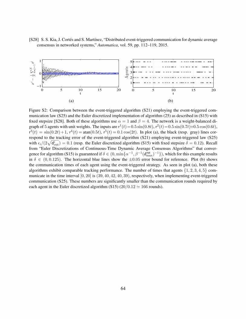
[S28] S. S. Kia, J. Cortes and S. Martınez, “Distributed event-triggered communication for dynamic averageconsensus in networked systems,” Automatica, vol. 59, pp. 112–119, 2015.

0 5 10 15 20

−1

0

1

xi−

1 N

∑N j=1rj

t

(a)

0 5 10 15 20

1

2

3

4

5

Agen

ts

t

(b)

Figure S2: Comparison between the event-triggered algorithm (S21) employing the event-triggered com-munication law (S25) and the Euler discretized implementation of algorithm (25) as described in (S15) withfixed stepsize [S28]. Both of these algorithms use α = 1 and β = 4. The network is a weight-balanced di-graph of 5 agents with unit weights. The inputs are r1(t)=0.5 sin(0.8t), r2(t)=0.5 sin(0.7t)+0.5 cos(0.6t),r3(t) = sin(0.2t)+1, r4(t) = atan(0.5t), r5(t) = 0.1 cos(2t). In plot (a), the black (resp. gray) lines cor-respond to the tracking error of the event-triggered algorithm (S21) employing event-triggered law (S25)with εi/(2

√diout) = 0.1 (resp. the Euler discretized algorithm (S15) with fixed stepsize δ = 0.12). Recall

from “Euler Discretizations of Continuous-Time Dynamic Average Consensus Algorithms” that conver-gence for algorithm (S15) is guaranteed if δ ∈ (0,min{α−1, β−1(dout

max)−1}), which for this example resultsin δ ∈ (0, 0.125). The horizontal blue lines show the ±0.05 error bound for reference. Plot (b) showsthe communication times of each agent using the event-triggered strategy. As seen in plot (a), both thesealgorithms exhibit comparable tracking performance. The number of times that agents {1, 2, 3, 4, 5} com-municate in the time interval [0, 20] is (39, 40, 42, 40, 39), respectively, when implementing event-triggeredcommunication (S25). These numbers are significantly smaller than the communication rounds required byeach agent in the Euler discretized algorithm (S15) (20/0.12 ' 166 rounds).

64

Authors Information

Solmaz S. Kia is an Assistant Professor of Mechanical and Aerospace Engineering at the Univer-sity of California, Irvine, CA, USA. She obtained her Ph.D. degree in Mechanical and AerospaceEngineering from UCI, in 2009, and her M.Sc. and B.Sc. in Aerospace Engineering from theSharif University of Technology, Iran, in 2004 and 2001, respectively. She was a senior researchengineer at SySense Inc., El Segundo, CA from Jun. 2009 to Sep. 2010. She held postdoc-toral positions in the Department of Mechanical and Aerospace Engineering at the UC San Diegoand UCI. She was a recipient of UC president’s postdoctoral fellowship in 2012-2014 and NSFCAREER award in 2017. Her main research interests, in a broad sense, include distributed opti-mization/coordination/estimation, nonlinear control theory, and probabilistic robotics.

Bryan Van Scoy is a postdoctoral researcher at the University of Wisconsin–Madison, WI, USA.He received the Ph.D. degree in Electrical Engineering and Computer Science from NorthwesternUniversity in 2017, and B.S. and M.S. degrees in Applied Mathematics along with a B.S.E. in Elec-trical Engineering from the University of Akron in 2012. His research interests include distributedalgorithms for multi-agent systems, and the analysis and design of optimization algorithms.

Jorge Cortes (M’02-SM’06-F’14) is a Professor of Mechanical and Aerospace Engineering at theUniversity of California, San Diego, CA, USA. He received the Licenciatura degree in mathematicsfrom Universidad de Zaragoza, Zaragoza, Spain, in 1997, and the Ph.D. degree in engineeringmathematics from Universidad Carlos III de Madrid, Madrid, Spain, in 2001. He held postdoctoralpositions with the University of Twente, Twente, The Netherlands, and the University of Illinoisat Urbana-Champaign, Urbana, IL, USA. He was an Assistant Professor with the Department ofApplied Mathematics and Statistics, University of California, Santa Cruz, CA, USA, from 2004 to2007. He is the author of Geometric, Control and Numerical Aspects of Nonholonomic Systems(Springer-Verlag, 2002) and co-author (together with F. Bullo and S. Martınez) of DistributedControl of Robotic Networks (Princeton University Press, 2009). He was an IEEE Control SystemsSociety Distinguished Lecturer (2010-2014) and is an IEEE Fellow. His current research interestsinclude cooperative control, network science, game theory, multi-agent coordination in robotics,power systems, and neuroscience, geometric and distributed optimization, nonsmooth analysis,and geometric mechanics and control.

Randy Freeman is a Professor of Electrical Engineering and Computer Science at Northwest-ern University, Evanston, IL, USA. He received the Ph.D. degree in electrical engineering fromthe University of California at Santa Barbara, Santa Barbara, CA, USA, in 1995. He has beenAssociate Editor of the IEEE Transactions on Automatic Control. His research interests includenonlinear systems, distributed control, multi-agent systems, robust control, optimal control, andoscillator synchronization. Prof. Freeman received the National Science Foundation CAREERAward in 1997. He has been a member of the IEEE Control System Society Conference EditorialBoard since 1997, and has served on program and operating committees for the American ControlConference and the IEEE Conference on Decision and Control.

65

Kevin Lynch (S’90-M’96-SM’05-F’10) is a Professor and the Chair of the Mechanical Engineer-ing Department, Northwestern University, Evanston, IL, USA. He received the B.S.E. degree inelectrical engineering from Princeton University, Princeton, NJ, USA, in 1989, and the Ph.D. de-gree in robotics from Carnegie Mellon University, Pittsburgh, PA, USA, in 1996. He is a memberof the Neuroscience and Robotics Laboratory and the Northwestern Institute on Complex Systems.His research interests include dynamics, motion planning, and control for robot manipulation andlocomotion; self-organizing multi-agent systems; and functional electrical stimulation for restora-tion of human function. He is a coauthor of the textbooks Principles of Robot Motion (MIT Press,2005), Embedded Computing and Mechatronics (Elsevier, 2015), and Modern Robotics: Mechan-ics, Planning, and Control (Cambridge University Press, 2017).

Sonia Martınez (M’02-SM’07-F’18) is a Professor of Mechanical and Aerospace Engineering atthe University of California, San Diego, CA, USA. She received the Ph.D. degree in EngineeringMathematics from the Universidad Carlos III de Madrid, Spain, in May 2002. Following a yearas a Visiting Assistant Professor of Applied Mathematics at the Technical University of Catalonia,Spain, she obtained a Postdoctoral Fulbright Fellowship and held appointments at the CoordinatedScience Laboratory of the University of Illinois, Urbana-Champaign during 2004, and at the Centerfor Control, Dynamical systems and Computation (CCDC) of the University of California, SantaBarbara during 2005. In a broad sense, her main research interests include the control of networksystems, multi-agent systems, nonlinear control theory, and robotics. For her work on the controlof underactuated mechanical systems she received the Best Student Paper award at the 2002 IEEEConference on Decision and Control. She was the recipient of a NSF CAREER Award in 2007. Forthe paper “Motion coordination with Distributed Information,” co-authored with Jorge Cortes andFrancesco Bullo, she received the 2008 Control Systems Magazine Outstanding Paper Award. Shehas served on the editorial boards of the European Journal of Control (2011-2013), and currentlyserves on the editorial board of the Journal of Geometric Mechanics and IEEE Transactions onControl of Network Systems.

66