two-tier labor markets in the great recession: …ftp.iza.org/dp5340.pdf · two-tier labor markets...
TRANSCRIPT

DI
SC
US
SI
ON
P
AP
ER
S
ER
IE
S
Forschungsinstitut zur Zukunft der ArbeitInstitute for the Study of Labor
Two-Tier Labor Markets in the Great Recession: France vs. Spain
IZA DP No. 5340
November 2010
Samuel BentolilaPierre CahucJuan J. DoladoThomas Le Barbanchon

Two-Tier Labor Markets in the
Great Recession: France vs. Spain
Samuel Bentolila CEMFI
Pierre Cahuc
Ecole Polytechnique, CREST and IZA
Juan J. Dolado Universidad Carlos III and IZA
Thomas Le Barbanchon
Ecole Polytechnique and CREST
Discussion Paper No. 5340 November 2010
IZA
P.O. Box 7240 53072 Bonn
Germany
Phone: +49-228-3894-0 Fax: +49-228-3894-180
E-mail: [email protected]
Any opinions expressed here are those of the author(s) and not those of IZA. Research published in this series may include views on policy, but the institute itself takes no institutional policy positions. The Institute for the Study of Labor (IZA) in Bonn is a local and virtual international research center and a place of communication between science, politics and business. IZA is an independent nonprofit organization supported by Deutsche Post Foundation. The center is associated with the University of Bonn and offers a stimulating research environment through its international network, workshops and conferences, data service, project support, research visits and doctoral program. IZA engages in (i) original and internationally competitive research in all fields of labor economics, (ii) development of policy concepts, and (iii) dissemination of research results and concepts to the interested public. IZA Discussion Papers often represent preliminary work and are circulated to encourage discussion. Citation of such a paper should account for its provisional character. A revised version may be available directly from the author.

IZA Discussion Paper No. 5340 November 2010
ABSTRACT
Two-Tier Labor Markets in the Great Recession: France vs. Spain* This paper analyzes the strikingly different response of unemployment to the Great Recession in France and Spain. Their labor market institutions are similar and their unemployment rates just before the crisis were both around 8%. Yet, in France, unemployment rate has increased by 2 percentage points, whereas in Spain it has shot up to 19% by the end of 2009. We assess what part of this differential is due to the larger gap between the dismissal costs of permanent and temporary contracts and the less restrictive rules regarding the use of the latter contracts in Spain. Using a calibrated search and matching model, we estimate that about 45% of the surge in Spanish unemployment could have been avoided had Spain adopted French employment protection legislation before the crisis started. JEL Classification: H29, J23, J38, J41, J64 Keywords: temporary contracts, unemployment, Great Recession Corresponding author: Pierre Cahuc Department of Economics Ecole Polytechnique 91128 Palaiseau Cedex France E-mail: [email protected]
* A preliminary version of this paper was prepared for the Fedea Annual Policy Conference, Madrid, 28-30 October 2009. We are very grateful to Florentino Felgueroso, J. Victor Rios-Rull, Gilles Saint-Paul, and Etienne Wasmer for their insightful suggestions that greatly improved the paper; useful comments are also acknowledged from participants at several seminars and conferences. We also wish to thank David Colino for excellent research assistance, and Brindusa Anghel and J. Ignacio García-Pérez for help with data.

1 Introduction
The goal of this paper is to explain the strikingly different response of Spanish unemploy-
ment relative to France, during the so-called Great Recession triggered by the financial
and economic crisis in 2007-08. We focus on a comparison with France because both
economies share similar labor market institutions (employment protection legislation, un-
employment benefits, wage bargaining, etc.) and exhibited very similar unemployment
rates, around 8%, just before the crisis started. However, while the French unemployment
rate has only risen to 10% during the slump, Spanish unemployment —after falling from
22% in 1994 to 8% in 2007, when Spain was creating a large share of all new jobs in the
European Union (EU)— has surged to 19% by the end of 2009. Our main contribution
in this paper is to analyze which part of this very different response can be attributed
to what we identify as the main difference between the labor market regulations of these
two economies: a larger gap between the dismissal costs of workers with permanent and
temporary contracts and a much laxer regulation on the use of temporary contracts in
Spain than in France. We argue that these differences, often ignored in cross-country
comparisons of overall employment protection legislation (EPL hereafter), could explain
up to 45% of the much higher rise of Spanish unemployment.
France and Spain allow us to tell an interesting tale of two neighboring countries. Both
are among those EU economies which most decidedly promoted temporary contracts in
the past to achieve higher labor market flexibility. Creating a two-tier labor market is
often seen as a politically viable way of achieving this goal when there is great resistance
from protected insider workers (see Saint-Paul, 1996 and 2000). However, temporary
employment is much more important in Spain, reaching around one-third of employees
until recently, whereas this share has been slightly below 15% in France. Therefore it seems
natural to ask whether the markedly different unemployment impact of the recession is
due to this difference, controling for other potential explanatory factors.
To explore these issues, following previous work by Blanchard and Landier (2002) and
Cahuc and Postel-Vinay (2002), we propose a search and matching model with endoge-
1

nous job destruction à la Mortensen-Pissarides (1994) which allows for the distinction
between permanent and temporary jobs. In our model, firms can offer both types of
contracts subject to different EPL, and the latter can be transformed into permanent
contracts at their expiration, the rest being terminated at low or no cost at all. It is now
well understood that facilitating the creation of temporary jobs promotes job creation but
increases job destruction, leading to an ambiguous effect on unemployment. However, one
result that has drawn less attention in this strand of the literature is that the increase
in job destruction induced by temporary jobs may have a larger adverse impact on un-
employment when the gap in firing costs in favor of permanent contracts is high enough.
The higher is this gap, the lower will be the proportion of temporary jobs transformed
into permanent jobs, because much larger firing costs for the latter induce employers to
use temporary jobs in sequence, especially if restrictions on their use are mild, rather than
converting them into long-term contracts. This implies that facilitating a widespread use
of flexible temporary contracts is more likely to raise unemployment in labor markets
already regulated by stringent permanent job security provisions.
The issue that labor market volatility increases with the introduction of flexible tem-
porary jobs has been stressed by Bentolila and Saint-Paul (1992) and Boeri and Garibaldi
(2007), who argue that two-tier labor market reforms have a transitional honeymoon, job-
creating effect which typically precedes reductions in employment as a result of temporary
workers’ lower labor productivity. Deepening this line of research, Sala et al. (2009) and
Costain et al. (2010) have recently studied the cyclical properties of dual labor markets
subject to limitations on the use of temporary contracts. In particular, they explore
whether flexibility at the margin is the reason why labor markets with a relatively high
degree of EPL may display similar volatility as fully flexible ones. While Sala et al. (2009)
find that this partial flexibility leads to an intermediate situation, in terms of unemploy-
ment volatility, between fully regulated and fully deregulated labor markets, Costain et
al. (2010), focusing on the Spanish case, estimate that unemployment fluctuates 22%
more in the prevailing dual labor market than it would in a unified economy with a sin-
2

gle contract. In common with these authors, our approach focuses on the interactions
between aggregate productivity shocks and EPL, including the regulation of temporary
jobs. However, while their work focuses on labor market dynamics over the business cycle
following a sequence of shocks, ours relies exclusively on a single shock which captures a
particularly relevant event, as is the case of the Great Recession. This simpler approach
has the advantage of enabling us to be more precise about the role played by specific
features of labor contracts that can account for the strikingly different response of France
and Spain to this global crisis.
From this perspective, our model differs from those of Sala et al. (2009) and Costain
et al. (2010) in three main respects. First, they assume that temporary jobs can be
destroyed at any time. However, since regulations impose that temporary jobs cannot
be destroyed before their date of termination, which is defined when the job is created,
our model accounts for this feature. Second, we assume that time is needed to destroy
permanent jobs, whereas they assume that these jobs can be instantly destroyed.1 Our
assumption is consistent with regulations which impose advance notice and induce delays
in job destruction due to the time needed to settle legal disputes. Third, we also differ
in how wage bargaining is modeled. In contrast with these authors, we do not assume
that employers have to pay firing costs if they do not agree on the initial wage contract
once they are matched with a worker. Instead, we assume that firing costs are paid
when workers and employers separate only if a contract has already been signed. As
Ljungqvist (2002) has shown, assuming that firing costs are paid by the employer if there
is a separation in the initial bargain —when the job starts— magnifies the impact of firing
costs on unemployment. We think that our assumption is more plausible and it captures
better the institutions of France and Spain, where labor contracts are renegotiated by
mutual agreement (Malcomson, 1999; Cahuc et al., 2006).
The rest of the paper is structured as follows. We start by documenting in Section 2
the relative performance of the French and Spanish labor markets during the crisis vis-à-
1 Garibaldi (1998) incorporated advance notice in a model with endogenous job destruction.
3

vis the preceding expansion. In Section 3 we present the main features of the regulations
affecting these two labor markets, devoting special attention to the EPL gap between
permanent and temporary contracts, and discuss how strong duality in labor markets can
affect sectoral specialization, labor mobility, and mismatch. In Section 4, we introduce a
stylized search and matching model focusing on equilibrium behavior of firms and workers
in an economy with both temporary and permanent contracts, where it is possible to
transform the former into the latter. In Section 5, we start by analyzing the extent to
which our calibrated model, with each country maintaining their respective prevailing
institutions before the slump, can account for the change in the performance of their
labor markets from the boom (represented by 2005-2007) to the recession (2008-2009),
following a common adverse shock affecting both economies. We then compute the share
of the rise in Spanish unemployment during the crisis which is due to differences in EPL
with France by running counterfactual simulations on how it would have fared had Spain
adopted French EPL before the recession started. Section 6 concludes.
2 Labor market performance before and during thecrisis
As depicted in Figure 1, France and Spain had an unemployment rate of 3.8% at the end
of 1976. From then on, both rates rose in tandem but the Spanish rate was always on top
and showed much higher volatility. The difference increased up until the end of 1994 and
shrank thereafter. By the end of 2005, the two unemployment rates seemed to have come
full circle, reaching similar values around 8%. Convergence was however a mirage. Since
the onset of the worldwide recession, unemployment in Spain has shot up from 8% to 19%
while French unemployment kept on falling, to 7.2%, and then has grown to 9.3%. In
the rest of this section, we briefly discuss some potential explanations for this strikingly
different response.
Table 1 presents a few key labor-market magnitudes from 1998:1 to 2007:4, an expan-
sion, and 2008:1-2009:4, a recession. It becomes apparent that, throughout the boom,
4
both labor force and employment growth rates have been much higher in Spain. It is the
Spanish figures that are remarkable, while the French ones are typical of the euro area
experience. While the share of foreigners in the French labor force was stable, the labor
force in Spain received a boost from large immigration flows amounting to around 1% of
the population per year, and also from an increase in the female labor participation rate
—for natives that rate increased by 8.4 percentage points (pp.) against 2.9 pp. in France.2
Focusing on private sector employees, it can be observed that the employment surge in
Spain stems especially from construction and market services (8.1% and 6.8% per year,
respectively). The corresponding figures were more moderate in France, including a fall
in manufacturing employment. The disparity was reinforced by the behavior of working
hours per employee: the implementation of the 35 hours law caused a significant drop in
France, while they were stable in Spain
In the downturn, growth in the French labor force has hardly altered, while in Spain it
has experienced a significant slowdown. France has suffered a small employment fall (0.3%
p.a.), though much more in terms of private sector employees (1.6%), which is dwarfed
by the Spanish free fall (4.6% p.a.), especially in the private sector (5.7%). The latter
stems especially from a collapse of almost 20% p.a. (i.e. 36% in total) of employment in
construction and a 10.8% drop in manufacturing.
As discussed earlier, it is very hard to explain the extreme volatility in the Spanish
labor market without recourse to the prevailing types of contracts. As shown in Table 1,
temporary contracts in 1998 represented almost 14% of employees in France and 33% in
Spain. During the expansionary period 1998-2007, the vast majority of (quarterly) flows
from unemployment to salaried employment were under these contracts: 78.4% in France
and 87.2% in Spain. Correspondingly, they also represented the majority of employment
outflows, in particular (from administrative sources): 88% in France and 80.1% in Spain.
Consequently, the brunt of job losses since the end of 2007 has been borne by temporary
jobs: 277.000 net jobs where destroyed in France, while actually 324.000 temporary jobs
2See Bentolila et al. (2008a) for a discussion of immigration flows in Spain.
5

disappeared, while the corresponding figures for Spain are simply stunning: 1.33 and 1.38
million jobs, respectively.
Table 1 also shows that the share of temporary jobs in Spain has slightly decreased,
from 33% to 31%, between 1998 and 2007. One may wonder how this matches with the
idea that the drop in unemployment is a result of the spread of temporary jobs over this
expansionary period. There are two explanations for this fact. On the one hand, this was
a very long expansion where Spanish GDP was growing at an average annual rate of 3.7%.
As pointed out by Wasmer (1999), such a long expansionary phase induces a so-called
capitalization effect whereby high growth increases future profits and thus strengthens
firms’ incentives to increasingly offer permanent contracts so as to retain their workers.
On the other hand, the Spanish government passed a labor reform in 1997 aiming to reduce
the severance pay gap between permanent and temporary contracts. They did so through
two new policy measures: a new type of permanent contract with lower severance pay
(see next Section), unavailable for males aged 31-44 years old unemployed for less than
one year, and the introduction of severance pay of 8 days of wages upon termination
of temporary and interim contracts (previously there was none). The 1997 reform also
included generous social security contribution rebates for hiring under the new permanent
contracts. Thus, in principle, the latter became more attractive. However, these changes
induced a very small drop in the rate of temporary employment, since the lower severance
pay does not apply to unfair dismissals for disciplinary reasons (e.g. worker misconduct),
which are the ones often employed by firms to avoid long and uncertain legal disputes
on the reason for the dismissals (see below). Therefore, even for these less-protected
contracts, firms ended up paying a high severance pay.3
3Indeed, Garcia-Perez and Rebollo (2009) document that, in practice, most firms use this contractto pocket the subsidy, usually dismissing the employee under the standard procedure, as soon as theminimum job duration required by law is reached.
6

3 Labor institutions in France and Spain
In this section, the institutional settings of the French and Spanish labor markets are
briefly reviewed. We focus on EPL, unemployment benefits and wage bargaining. We
argue that the main difference arises from the higher EPL gap between permanent and
temporary workers in Spain than in France. Finally, we examine labor mobility, which we
document to be much lower in Spain, partly as a result of the high uncertainty associated
with the use of temporary contracts and the low conversion rates to permanent ones
induced by the large EPL gap.
3.1 Employment protection
As mentioned earlier, France and Spain are among the countries where governments have,
through their regulations, more strongly promoted temporary contracts to increase labor
market flexibility aimed at reducing unemployment.
Table A1 in the Appendix presents the key features of regulations concerning dis-
missals in the two countries. Permanent contracts are subject to advance notice periods
and severance pay.4 Severance pay for economic reasons in France is equal to 6 days
of wages per year of service (the latter clause is understood hereafter) plus 0.08 extra
days for tenure above 10 years. In Spain that pay is equal to 20 days, whereas severance
pay for unfair dismissal is equal to 45 days. From these figures it may seem that firing
permanent employees is much cheaper in France than in Spain, but this would be mislead-
ing, since there are additional important components of firing costs beside severance pay.
For example, in France, as soon as a worker reaches a 2-year seniority the notice period
doubles, while in Spain most firms avoid it in exchange for a much higher severance pay.
Likewise, administrative approval is required for collective dismissals in Spain (roughly
4In France, this includes the regular permanent contract or contrat à durée indeterminée (CDI) andthe new employment contract (contrat nouvelles embauches, CNE, which has different severance payand other conditions) introduced in 2005 for small firms (see Cahuc and Carcillo, 2006). In Spain itincludes both regular permanent contracts and the subsidized contrato indefinido de fomento del empleoIn principle, the latter has lower severance pay but, as argued above, in fact most dismissals incur thepenalty rate for unfair dismissals.
7

those involving 10% of an establishment’s staff), which is almost impossible to obtain
without worker representatives’ agreement to the dismissal in advance (again in exchange
for higher severance pay).
Computing overall measures of EPL is not an easy task. Let us consider the widely
used OECD (2004) index of the strictness of EPL for 2003, which ranges from 0 to 6, with
higher scores indicating stricter regulation. This indicator gives a score of 2.5 for France
and 2.6 for Spain regarding protection of permanent jobs, 3.6 for France and 3.5 for Spain
on regulation of temporary jobs, and 2.1 for France and 3.1 for Spain on regulation of
collective dismissals. The overall EPL score is 3.0 for France and 3.1 for Spain (where
the US has the lowest value, 0.7, and Portugal and Turkey the highest, 4.3). Hence,
both countries are ranked in the middle-high range, with Spain appearing only slightly
more regulated than France. However, there are good reasons to think that this average
EPL index, based on legal regulations and not on their implementation, does not capture
Spanish EPL satisfactorily. As argued below, de facto EPL of temporary jobs is much
weaker in Spain than in France, whereas the opposite holds for EPL of permanent jobs.
Moreover, economic theory on the effects of firing costs on employment tells us that
what matters is not severance pay per se, which is a transfer from the firm to the worker
and may therefore be compensated for in the wage bargain (Lazear, 1990). Rather, since
the probability that workers will contest dismissals is very high, what matter are other
costs that are not appropriated by firms and workers but are generated by third agents,
such as labor courts and labor authorities, i.e., the so-called red-tape costs. For example,
severance pay offered by firms in exchange for a quick resolution of dismissals in France is
typically higher than statutory severance or that agreed in collective bargains. In Spain,
the extra cost does not only apply to collective dismissals but also to individual ones.
In effect, since firms that go to court lose in 3 out of 4 cases on average, they typically
find it more profitable to allege disciplinary reasons even if they think that dismissals are
justified on economic grounds. Proceeding in this way they do not need to satisfy the
notice period and, upon immediately acknowledging the dismissal to be unfair, they avoid
8

going to court by paying upfront the penalty of 45-days severance pay.5 In applying our
theoretical model to these two labor markets, we adopt a conservative strategy and only
focus on the distortionary effect of the firing tax component of severance pay. Accordingly,
we will use estimated red-tape costs which, as will be discussed in Section 5.2, turn out
to be 50% higher in Spain than in France, though the notice period is much shorter, an
EPL feature also accounted for in our calibrated model.
Further, the use of temporary contracts is rather more limited in France than in Spain.6
In France, they can only be used in nine specific cases: for replacing an employee who is
absent or temporarily working part time, to transitorily replace an employee whose job is
either going to be suppressed or filled by another permanent worker, and for temporary
increases in the firm’s activity, seasonal activities, and jobs in certain sectors (forestry,
naval, entertainment, teaching, survey-making, professional sports, etc.). In Spain, tem-
porary contracts may be used for objective reasons (specific work, accumulation of tasks,
replacement, etc.), for training, to hire disabled workers, and to cover the part of the
working day left uncovered by an employee close to retirement. De facto, however, there
are no restrictions: employers are hardly monitored by the authorities to ensure that they
comply with the alleged reasons for hiring under temporary contracts. Finally, while in
both countries the maximum duration of temporary contracts is 24 months, uncertain-
completion jobs (e.g., in the much more prominent construction sector in Spain before
the crisis) may lawfully last for an indeterminate period.
In sum, the previous discussion points out that, in contrast with OECD rankings, EPL
for permanent contracts is more stringent in Spain than in France, while the opposite is
true for temporary contracts. Thus overall EPL may look similar but this aggregate
5This option has been available to firms in Spain since the Law 45/2002 was passed and it impliesseverance payments of 45 days of wages per year of service, with a maximum of 42 months’ wages.
6In this paper we use the term “temporary contracts” to denote all sorts of non-permanent contracts.We focus on fixed-term contracts, captured by the contrat a duration determinée (CDD) in France andthe contrato temporal in Spain. There are several types of temporary contracts in Spain. And other non-permanent jobs exist in France, such as temporary jobs proper (emploi interimaire or emploi temporaire).Moreover, in both countries there are also jobs intermediated by temporary work agencies and mostapprenticeship contracts are temporary as well. Empirically we shall consider all of these as temporarycontracts.
9

indices hide the fact that the gap in EPL between the two types of contracts turns out to
be much higher in Spain.7 ,8
3.2 Unemployment benefits
Unemployment insurance in France features a gross replacement ratio of 57.4% of the
preceding year’s wage.9 In Spain, the replacement ratio decreases over time: it is 70%
for the first 6 months and drops to 60% thereafter. Thus, at least at the beginning of
unemployment spells, the Spanish system looks more generous than the French one. In
comparing benefits, however, it is crucial to take into account personal characteristics and
to consider replacement rates net of taxes. Thus, according to the OECD Benefits and
Wages database (March 2006 update), the net replacement rate in 2004 for an average
production worker who was married, whose partner did not work, and who had no children
was equal to 69% in both countries. Likewise, if the same worker was married with a
working partner and had two children, again the replacement rates do not differ much:
84% in France and 87% in Spain.
In France, the length of benefits is the same as the worker’s contribution period, with
a maximum duration of 23 months (and higher for workers older than 50 years old). In
Spain, benefit length increases in steps that imply durations going from 22% to one-third of
the contribution period, which has to be of at least 12 months, with a maximum duration
of 24 months. In computing a measure of unemployment benefits for our simulations we
take into account statutory benefits and coverage, which is affected by duration rules.
Workers who exhaust unemployment insurance or are ineligible for it are entitled to
so-called “minimum integration income” (Revenu Minimum d’Insertion, RMI) in France,
amounting to €454.63 (the minimum wage net of social contribution for full time work-
7For more specific details on the level and structure of firing costs in France, see Cahuc and Postel-Vinay (2002) and Cahuc and Carcillo (2006), and Bentolila and Jimeno (2006) and Bentolila et al. (2008b)for Spain.
8A labor market reform has been approved in Spain in September 2010, which has altered severancepay for permanent and temporary contracts. This reform is however outside the period we examine andits effects will only be felt over time.
9Or, if it is higher, 40.4% of the wage plus a fixed amount (currently around 330 euros per month).
10

ers being equal to €1,042) and €681.9 for a couple (plus child benefits).10 In Spain, the
assistance benefit is equal to 80% of the so-called “Multi-Purpose Public Income Indi-
cator”, which in 2008 amounted to €413.5 (around 23% of gross earnings in the private
non-agricultural sector), with higher benefits for workers with family responsibilities. It is
means-tested at the level of the benefit. Additional welfare benefits are available in some
regions (for example in Madrid they amount to €370) but coverage is typically low.
3.3 Wage bargaining
Collective wage bargaining is similar in the two countries. It can be argued that this
is the result of Spain adopting French regulations in the early 1980s, when the post-
dictatorship Spanish system of collective bargaining was established. In both countries,
most workers are covered by collective bargaining, above 90% in France and above 80%
in Spain. Bargaining takes place mostly at the industry level and there is geographical
fragmentation (through industry-department agreements in France and industry-province
agreements in Spain). Conditions set in above firm-level agreements are extended to all
firms and workers in the relevant industry or geographical area; extension is discretionary
in France and automatic in Spain.
In Spain, workers are represented by worker delegates in firms with less than 50 em-
ployees and by worker committees in firms with more than 50 employees, reflecting French
practice. Unions obtain representation from firm-level elections, where voters need not be
unionized. Thus, there is little incentive for workers to unionize, so that union density is
very low but largely irrelevant. Both countries have the highest gaps between the coverage
of collective bargaining and union density (in 2007 the latter was equal to 8% in France
and 14.6% in Spain, see Visser, 2009).11 One difference, though, is that whereas in Spain
there are only two nationally representative unions (CCOO and UGT), in France there
10The RMI was replaced, as of the third quarter of 2009, by the Revenue de Solidarité Actives (rSa).There is another scheme equivalent to the RMI (also open to those above 25 years old who never worked)for those who have worked before and are not eligible anymore: the Allocation de Solidarité Specifique(ASS), with an amount equivalent to the RMI.11For more details regarding Spain see Bentolila and Jimeno (2006).
11

are eight unions. Nonetheless, they are not equally powerful and, like in Spain, two unions
are especially influential, particularly in the public sector (CGT and CDFT). Lastly, it
is worth noting that, although the monthly statutory minimum wage is quite higher in
France than in Spain (1,321 and 728 euros in 2009, respectively; Eurostat), the Kaitz ratio
(i.e., the ratio between the minimum and the average wage) is not very different (41% and
50% respectively). Moreover, fewer full-time workers receive the minimum wage in Spain
(about 5% and 18%, respectively) because wage floors are often determined in collective
bargaining above the statutory level.
In sum, we believe that the two countries are not significantly different in their wage
setting institutions and therefore we do not explore any potential differences in this di-
mension in the simulations below.
3.4 Mismatch, sectoral specialization and labor mobility
Besides the EPL gap, labor mobility is the other dimension in which the French and
Spanish labor markets differ.12 This difference does not become apparent in job mobility,
which turns out to be rather similar: average job duration is equal to 7.6 years in France
and 8.2 in Spain, while the fractions of workers who have changed job in the preceding
10 years are 49% and 50%, respectively.13
Yet, geographical mobility is much lower in Spain. A good starting point in docu-
menting this difference is home leaving. The average age at which young people leave the
parental home in France is around 24 years old against around 29 years old in Spain. An-
other striking disparity is that the fraction of people who have never moved after leaving
the parental home is equal to 23% in Spain but only 8% in France. Moreover, while 30%
of the French population has moved across regions, only 11% of Spaniards have done so.
Overall, the interregional migration rate for people aged 15-64 is 2.1% in France and only
0.2% in Spain, with a wider disparity for young people (15-24 years old): 3.8% in France
12We are very grateful to Etienne Wasmer for suggesting that we take this issue into account.13This is in spite of the higher temporary employment rate in Spain, due to its higher EPL on permanent
jobs vis-à-vis France.
12

and 0.23% in Spain.14
Low interregional mobility has affected the impact of the recession in Spain, since its
regions have been hit quite differently by the crisis. Regional employment destruction
growth rates of dependent employment, which range from -1% to -13.4% (2007:4-2009:3),
are closely related to the regional shares of employment in the construction industry, which
has plummeted during the recession (a 36% nationwide reduction of employment in this
sector with regional rates ranging from 18.7% to 54.7%). This strong link is illustrated by
the raw correlation coefficient between the changes in total and construction employment
shares across Spanish regions, which is equal to 0.7.15
In what follows we argue that the strong dependence of the Spanish economy on the
construction sector since the late 1990s (11.9% of GDP and 13.3% of employment in 2007,
against 6.3% and 6.9% in France; Eurostat) is closely related to the existence of a dual
labor market. In effect, as a result of Spain’s access to the euro area in the late 1990s
with a higher inflation rate than France, real interest rates fell by 6 pp., against 1.5 pp.
in France, fueling a strong investment boom. These new investment projects could have
taken place in either high value-added industries (like, e.g., ICT in Finland) or in low-value
added ones. Investors bet rationally for the latter for at least two reasons. On the one
hand, the rigid permanent contracts would have been inadequate to specialize in more
innovative sectors, since higher labor flexibility is required to accommodate the higher
degree of uncertainty typically associated with producing higher value-added goods (Saint-
Paul, 1997). On the other hand, there was a large increase in the relative endowment
of unskilled labor in Spain over that period. The higher availability of low-skilled jobs
through very flexible contracts since the mid-1980s led to a high dropout rate of youth
from compulsory education (from 18% in 1990 to 32% in 1997) and subsequently to a huge
inflow of unskilled immigrants (implying a 10 pp. increase in the foreign population rate).
14The home-leaving figure corresponds to 2007, from the Labor Force Survey, see Eurostat (2009),Figure 2.1. The subsequent figures are for 2005, from the analysis of the 2005 Eurobarometer by Van-denbrande et al. (2006), Figures 20, 23, 2 and 3, and Table 2, respectively. Lastly, the interregionalmigration rate corresponds to 2003, from OECD (2005).15These figures leave out the Balearic Islands, which have an abnormally high employment level in
2009:3 due to seasonal factors related to the turism industry.
13

Hence, as a result of this relative abundance of less-skilled labor, most firms, especially
small and middle-sized ones, adopted technologies which where complementary with this
type of workers, leading to a boom in the construction sector.
Low geographical mobility is a source of mismatch and higher equilibrium unemploy-
ment via reallocation rather than conventional aggregate shocks (Layard et al., 1991).
This has become quite apparent in the aftermath of the recession in Spain, where unem-
ployment rate dispersion has sharply increased. The range between the lowest and the
highest regional unemployment rates, which was equal to 10.3 pp. in 2007:4, has risen to
15.6 pp. in 2009:4, whereas the standard deviation of those rates increased from 3 to 5
over that period.16 In sharp contrast, that range only increased in France from 9.6 pp. to
11.3 pp., while the standard deviation hardly changed, from 1.3 to 1.4.17
Geographical mobility depends on many factors, both economic and non-economic. In-
stitutional determinants of regional divergence in incomes and unemployment rates surely
play a role. For instance, Bentolila and Dolado (1991) found, for 1962-1986 (roughly a
pre-temporary employment period in Spain), that if the national unemployment rate dou-
bled (from 10% to 20%, not far from the current situation), the elasticity of interregional
migration flows to regional wage and unemployment differentials halved. This estimate
is likely to be similar nowadays. On the other hand, Rupert and Wasmer (2009), echoing
earlier work by Oswald (1999), highlight the role of housing regulations in accounting
for differences in unemployment between Europe and the US. The Spanish rental market
works very poorly and is underdeveloped, representing only 12% of the housing market,
against 40% in France. Therefore, it clearly hampers regional migration (Barceló, 2006).
This is due to various institutional factors, in particular a legal structure that favors ten-
ants vs. landowners and an income tax system which heavily subsidizes owner-occupied
housing (Lopez-Garcia, 2004).
Moreover, like in the case of industrial specialization, differences in EPL may be a
16This was even stronger for workers aged 16 to 24 years old. The lowest-highest unemployment ratedifference increased from 19.4 to 24.7 and the standard deviation from 4.6 to 6.3.17France: Labor Force Survey, BDM Macro-economic Database (www.bdm.insee.fr). Spain: Labor
Force Survey (www.ine.es).
14

concomitant event to differences in labor mobility. On the one hand, there is evidence
that the widespread use of temporary contracts may reduce regional migration despite its
potentially beneficial effect on job creation. For example, using individual data for Spain,
Antolín and Bover (1997) found that temporary employment reduces the likelihood of
interregional migration. The insight is that a temporary job in a different region does
not provide much job security whereas migrating means giving up, to a large extent, the
support of family networks, which are a key insurance mechanism in Southern Mediter-
ranean countries (Bentolila and Ichino, 2008). In a similar vein, Becker et al. (2010)
find, with a sample of 13 European countries over 1983-2004, that youth job insecurity
discourages home-leaving, whereas parental job insecurity encourages it. Thus, to the
extent that permanent and temporary contracts are roughly held by older and younger
workers, respectively, the much higher EPL gap in Spain would be consistent with its
much lower home-leaving rate.
Overall, the above evidence indicates that the Great Recession is likely to have induced
a much larger increase in mismatch in Spain than in France. Indeed, the Spanish Beveridge
curve, plotted in Figure 2, confirms that this differential effect may have been rather
relevant. While there seems to be a stable relationship from 1994 to 2007, there is a large
outward shift during the Great Recession of both the vacancy rate and the unemployment
rate, indicating growing mismatch.18 For France, data are not available on vacancy stocks,
only on flows. Yet, though not reported (but available upon request), unlike in Spain,
these flows show no indication, of an outward shift in the French Beveridge curve from
1997 until 2009.
4 Model
This section presents our search and matching model, inspired by previous work by
Blanchard and Landier (2002) and Cahuc and Postel-Vinay (2002), where the seminal18Unemployment is expressed as a percentage of the labor force whereas vacancy is in per thousand.
The figures in the graph are adapted from results in Bouvet (2009) spliced with survey data from theEncuesta de Coyuntura Laboral (www.mtin.es/estadisticas/ecl/Ecl22010/SER/index.htm), which startin 2000.
15

Mortensen-Pissarides (1994) model with endogenous job destruction is extended to allow
for the distinction between temporary and permanent jobs entailing different dismissal
costs and advance notice periods.
4.1 Model setup
The main features of the model are as follows. First, there is a continuum of infinitely-
lived risk-neutral workers and firms, with a common discount rate r > 0. The measure of
workers is normalized to 1.
Job matches have an idiosyncratic productivity distribution F (ε), drawn over the
support [ε, ε].19 The idiosyncratic productivity shocks follow a Poisson distribution with
incidence rate μ. In line with Pissarides (2000), it is assumed for simplicity that all new
jobs start at the highest productivity ε.20
There are two types of jobs, temporary and permanent, both endowed with the same
productivity distribution. Trying to mimic realistic wage bargaining procedures, it is
assumed that wages are only renegotiated in permanent jobs but not in temporary jobs,
where wages are often fixed for the whole duration of the contract. Unemployed workers
have access to temporary jobs with probability p, exogenously set as EPL policy, and to
initial permanent jobs with probability (1− p). Temporary jobs are terminated with perunit of time probability λ, at which point firms can either convert them to permanent jobs
or destroy them at no cost. A new value of productivity is drawn when the conversion
takes place.
There are two constraints to destroy permanent jobs. First, there are red-tape firing
costs f , to be directly interpreted as the EPL gap under the previous assumption that
termination of temporary contracts entail no red-tape firing costs. Secondly, time is needed
to destroy permanent jobs: when an employer wishes to destroy this type of jobs, there
19We introduce an aggregate shock, which corresponds to the Great Recession, rather than a sequenceof shocks as in L’Haridon and Malherbet (2009), Costain et al. (2010), or Sala et al. (2010).20This assumption reduces the number of productivity cutoff levels to just two (see equation PJD and
PJC below) which simplifies considerably the analysis and calibration of the model, without qualitativelyaffecting its main implications.
16
is a firing permission which arrives at a Poisson rate σ (Garibaldi, 1998). This firing
permission typically captures not only advance notice, but also the uncertain time needed
to settle legal disputes. Between the date at which the employer decides to destroy the
job and the date at which the authorization arrives, we assume that the productivity of
the job is lowest possible, i.e., equal to ε , and that the interim wage equals the average
wage in the economy, ω (see the definition below) capturing in this fashion a prototypical
employment record in this economy.
Unemployment benefits are denoted by b. Note that both firing costs and unemploy-
ment benefits should be interpreted as monetary flows in terms of the average wage, i.e.,
as fω and bω, though for short they will be respectively referred to as f and b hereafter.
There is a Cobb-Douglas matching functionm(u, v) = m0uαv1−α à la Pissarides (2000),
with matching rates q(θ) for vacancies and θq(θ) for the unemployed. Thus, labor market
tightness is given by θ = v/u, where v and u are the masses of vacancies and unemploy-
ment, respectively. The degree of mismatch is captured by the shifter m0 such that a
lower value of m0 signifies higher mismatch, that is, an outward shift in the Beveridge
curve. Finally, there is a flow cost of keeping jobs vacant equal to h > 0 per unit of time.
In terms of notation, subindices are as follows: t stands for a temporary job, 0 for the
beginning of a permanent job, p for a continuing permanent job, and a for jobs that wait
for the authorization to be destroyed.
Asset values at steady state are denoted J and V for employers, and W and U for
employees. They are as follows:
• V : Value to the firm of a vacant job,
• Jt(ε): Value to the firm of a temporary job with productivity ε,
• J0(ε): Value to the firm of a new permanent job with productivity ε, not yet subjectto firing costs,
• Jp(ε): Value to the firm of a continuing permanent job with productivity ε, subject
to both firing cost f and advance notice
17

• Ja : Value to the firm of a permanent job under advance notice,
• U : Value to the worker of unemployment,
• Wt(ε): Value to the worker of a temporary job with productivity parameter ε,
• W0(ε): Value to the worker of a new permanent with productivity ε subject to firing
costs f (recall that a new permanent job can previously be a temporary job),
• Wp(ε): Value to the worker of a continuing permanent job with productivity para-
meter ε, subject to firing costs f .
• Wa : Value to the worker of a permanent job under advance notice.
4.2 Bellman equations
The Bellman equations for the firm’s asset values are as follows:
rV = −h+ q (θ) [p (Jt(ε)− V ) + (1− p) (J0(ε)− V )] (1)
rJt(ε) = ε−wt+μ
Z ε
ε
[Jt(x)−Jt(ε)]dF (x)+λ
Z ε
ε
max[J0 (x)−Jt(ε), V −Jt(ε)]dF (x) (2)
rJ0(ε) = ε− w0 (ε) + μ
Z ε
ε
max[Jp (x)− J0(ε), Ja − J0(ε)]dF (x) (3)
rJp(ε) = ε− wp (ε) + μ
Z ε
ε
max[Jp (x)− Jp(ε), Ja − Jp(ε)]dF (x) (4)
rJa = ε− ω − σ [f + Ja − V ] (5)
According to (1), keeping a vacant job implies a flow cost of h and returns a contact
with probability q(θ) in each period. Once the contact takes place, the employer-employee
pair sign a temporary contract with probability p or a new permanent contract with
probability 1 − p, both created at the maximal productivity level, ε. If a temporarycontract is signed, equation (2) implies that the employer obtains a flow profit of ε−wt,where wt is the pre-established wage for this type of contracts which does not depend
on productivity. After the productivity shock takes place, at rate μ, this type of job
18

—which yields an asset value to the employer of Jt(ε)— necessarily continues until the
arrival of the date at which it can be destroyed. This assumption reflects the fact that
employers are not allowed to layoff workers on temporary contracts before the end of the
contract. Temporary contracts are terminated at rate λ.21 When a temporary contract
is terminated, the job can be either destroyed or converted into a permanent job. At the
date of the termination of the temporary contract, a new value of the productivity shock
is drawn in line with available evidence pointing out that workers’ productivity may be
different under permanent and temporary contracts.22
The asset value to the employer of a new permanent job, filled either by an unemployed
worker or by a worker on a temporary contract, is J0(ε) which, according to (3), yields
a flow profit of ε − w0 (ε). Once a productivity shock occurs at rate μ, the permanent
contract becomes a continuing one —with an asset value to the firm of Jp(ε)— if the employer
decides to keep the job, or it becomes a job under advance notice —with an asset value of
Ja, if the employer prefers to fire the worker. Equation (4) indicates that the employer
with a continuing job obtains a flow profit of ε−wp (ε), such that the only difference withthe value of a new job —defined by equation (3)— is that the worker can now use both
the firing cost and the advance notice, Ja, as additional threats in the wage bargain. As
mentioned earlier, it is assumed that jobs under advance notice, whose value is defined by
equation (5), have the lowest possible productivity ε and pay workers the average wage.
These assumptions are a simple way to account for the fact that workers under advance
notice generally provide low work effort and are paid a wage that depends on their past
remuneration. Lastly, (5) also indicates that jobs under advance notice can be destroyed
at an incidence rate σ.
Turning now to workers, their corresponding Bellman equations are given by:
rU = b+ θq(θ)[ p(Wt(ε)− U) + (1− p)(W0(ε)− U)] (6)
21Assuming that the duration of temporary contracts is fixed rather than random leads to more complexformulations without changing the properties of the model.22For example, Ichino and Riphahn (2005) have shown that the number of days of absence per week
increases significantly once employment protection is granted at the end of probation periods.
19

rWt(ε) = wt + μ
Z ε
ε
[Wt(x)−Wt(ε)]dF (x) + λ
Z ε
ε
max[W0 (x)−Wt(ε), U −Wt(ε)]dF (x)
(7)
rW0(ε) = w0 (ε) + μ
Z ε
ε
max[Wp (x)−W0(ε),Wa −W0(ε)]dF (x) (8)
rWp(ε) = wp (ε) + μ
Z ε
ε
max[Wp (x)−Wp(ε),Wa −Wp(ε)]dF (x) (9)
rWa = ω + σ [U −Wa] (10)
Equation (6) shows that an unemployed worker enjoys a flow earning b and gets in
contact with a vacancy at rate θq(θ), either of a temporary job or of a new permanent
job, with probabilities p and 1−p, respectively. Expressions (7) to (9) represent the assetvalues to the worker of the different jobs, and their interpretation is similar to those in
(2) to (4) with the flow income being the respective wages. Finally, (10) represents the
asset value to the worker of being dismissed from a non-temporary job.
4.3 Surplus sharing
As is conventional in this type of models, the surplus is shared according to a Nash
bargain in which workers have bargaining power β ∈ [0, 1]. This gives rise to the surplusexpressions:
St(ε) = Jt(ε)− V +Wt(ε)− U (11)
S0(ε) = J0(ε)− V +W0(ε)− U (12)
Sp(ε) = Jp(ε)− Ja +Wp(ε)−Wa (13)
where the surplus for temporary jobs is defined at it initial productivity level, ε, and those
of permanent jobs at the date where the new productivity shock ε arrives.
Since we have
Wa + Ja =ε+ σ (U − f + V )
r + σ
the surplus of continuing permanent jobs can be rewritten as
Sp(ε) = Jp(ε)− V + f +Wp(ε)− U −µε− r (U − f − V )
r + σ
¶(14)
20

The free-entry rule V = 0 implies:
h = q (θ) [pJt(ε) + (1− p)J0(ε)] (15)
Therefore, since Ji(ε) = (1− β)Si(ε), i = t, 0, we get:
θh
1− β= θq (θ) [pSt (ε) + (1− p)S0(ε)] (16)
Bargaining, together with free entry, implies:
W0(ε)− U = βS0(ε)
J0(ε) = (1− β)S0(ε)
Wp(ε)−Wa(w) = βSp(ε)
Jp(ε)− Ja(w) = (1− β)Sp(ε)
From (12) and (13):
Sp(ε) = S0(ε) +1
r + σ
µσf + b+ θ
βh
1− β− ε
¶where rU + σf − ε = b+ θ βh
1−β + σf − ε > 0 to ensure job destruction. Thus, the surplus
from a continuing permanent job is larger than the surplus from a new permanent job,
due to our previous assumption that the employer only has to pay the firing cost and to
comply with the advance notice if the worker has been confirmed in the job and not when
disagreement arises at the time of the first encounter with the worker.
4.4 Job creation and job destruction
The previous expressions for the surpluses yield the productivity thresholds used by firms
for the destruction of permanent jobs (PJD) and the creation of permanent jobs (PJC):23
Sp(εd) = 0 = εd − r
r + σ(ε− σf)− σ
r + σ
µb+ θ
βh
1− β
¶+ μ
Z ε
εdSp(x)dF (x) (PJD)
S0(εc) = 0 = εc +
μ
r + σ(ε− σf)− r + σ + μ
r + σ
µb+ θ
βh
1− β
¶+ μ
Z ε
εdSp(x)dF (x) (PJC)
23Notice that the job creation threshold does not exist for jobs filled by unemployed workers, sincethese jobs are created at the maximal productivity.
21

Hence, subtracting (PJD) from (PJC) yields:
εc = εd +r + μ
r + σ
µσf + b+ θ
βh
1− β− ε
¶(17)
which shows that temporary jobs are destroyed more frequently than continuing perma-
nent jobs, because they are exempt from firing costs. Moreover, the wedge between εc
and εd increases with f and σ.
From the expressions for Sp(ε), S0(ε), Sp(εd), and S0(εc), we get the following relations:
S0(ε) =ε− εc
μ+ rfor ε ≥ εc (18)
Sp(ε) =ε− εd
μ+ rfor ε ≥ εd (19)
where (18) and (19) can be replaced into (PJD) to derive the following productivity
threshold for the destruction rule of permanent jobs:
εd =r
r + σ(ε− σf) +
σ
r + σ
µb+ θ
βh
1− β
¶− μ
μ+ r
Z ε
εd
¡x− εd
¢dF (x) (20)
This equation shows that the threshold productivity εd is an increasing function of
labor market tightness, θ, and a decreasing function of the firing cost, f .24 The intuition
for the first relationship is that a tighter labor market, by improving the value of unem-
ployment U , reduces the surplus, thus making the employer-worker pair more exacting
on how productive the match must be to compensate them for their outside options. As
regards the second relationship, it is consistent with the goal of firing costs of reducing
the propensity to destroy jobs, implying that less productive jobs remain operative.
Moreover, (11) implies that
(r + λ)
Z ε
ε
St(x)dF (x) =Z ε
ε
xdF (x)− b− βθh
1− β+ λ
Z ε
εc
ε− εc
μ+ rdF (x)
and then,
St(ε) =1
(r + μ+ λ)
∙ε+
μ
r + λ
Z ε
ε
xdF (x)¸+
1
r + λ
∙λ
Z ε
εc
x− εc
μ+ rdF (x)− b− βθh
1− β
¸(21)
24It can be also shown to be an increasing function of the average duration of the advance notice period(1/σ), for values of f sufficiently large, since sign(∂εd/∂σ) =sign(rU − ε − rf). The intuition for thisresult is that, since the firm anticipates more firing restrictions when conditions are bad, it becomes moreexacting (higher εd) as advance notice increases (as σ falls).
22

Evaluation of both (21) and (18) at ε yields St(ε) and S0(ε), respectively, which can
be then used to rewrite the overall job creation equation (JC) out of the free-entry rule
as follows:
h
1− β= q (θ)
"p
(r+μ+λ)[ε+ μ
r+λ
R ε
εxdF (x)] + p
r+λ[λR ε
εc(x−εc)μ+r
dF (x)− b− βθh1−β ]
+(1− p) ε−εcμ+r
#(JC)
By replacing εc by εd in equation (JC), using equation (17), it is easy to show that,
along the JC locus, labor tightness θ is a decreasing function of the job destruction
productivity cutoff εd. In other words, the lower the destruction threshold εd, the longer
jobs last on average, which leads to a higher creation of vacancies. Conversely, for a given
value of εd, a higher firing cost f reduces the expected present value of jobs and therefore
hinders job creation.
In sum, besides the unemployment rate (see below), the steady-state equilibrium values
of the other three unknowns in our model, θ, εc, and εd, are found by solving the system
of equations given by (JC), (17) and (20). Equilibrium is depicted in Figure 3, where the
crossing of the JC (having replaced εc by εd) and PJD loci in the (θ, εd) space determines
the equilibrium values of these two variables, whereas (17) determines the equilibrium
value of εc. In Figure 4 we consider the effect of an increase in the firing cost gap between
permanent and temporary workers. This is captured by a rise in f , which shifts the PJD
and JC schedules downwards and the PJC locus upwards.25 Firms unambiguously fire
less permanent workers (lower εd), transform temporary contracts into permanent ones
less frequently (higher εc), and reduce labor market tightness (θ) for given values of the
productivity thresholds. Although in principle the conventional ambiguity on the effect of
firing costs on unemployment holds, as a result of the lower job creation and destruction
rates, it will be shown below that, in a dual labor market which initially exhibits a high
gap in firing costs, a further increase in f will raise unemployment. The intuition is that, if
the conversion rate from temporary to permanent contracts is low to start with, a further
rise in f exacerbates temporary workers’ turnover precisely when less vacancies are being
25>From equations (17) and (20), we get dεc
df
¯θ=ctant
= μF (εd)1− μ
μ+r [1−F (εd)] > 0.
23

created. Thus, unemployment is likely to go up, as Blanchard and Landier (2002), and
Cahuc and Postel-Vinay (2002) have pointed out before.
Figure 5, in turn, shows the effect of a reduction in p, an EPL policy parameter which,
as mentioned earlier, is bound to be higher in Spain than in France because the laxer
restrictions in the use of temporary contracts and the higher weight of the construction
sector in Spain before the current recession. Now, the PJC and PJD loci remain unaffected
whereas the JC schedule shifts downwards, since job creation is hindered by the lower
availability of flexible contracts. As a result, the equilibrium value of θ unambiguously
decreases whereas the two productivity cutoff values fall. In other words, since decreasing
p lowers job creation, firms become less exacting about hiring and firing, making job
turnover less intensive. As a result, despite the fall in θ, the impact of a reduction of
p on the unemployment rate is ambiguous. However, like before, if the economy has a
large firing costs to start with, a reduction in p is likely to decrease temporary workers’
turnover, and this may reduce unemployment, as our quantitative simulations below show.
Finally, it is straightforward to check that either a rise in λ (i.e. a higher frequency in
the termination of temporary jobs) or a reduction in m0 (i.e. an increase in mismatch)
unambiguously lead to lower θ and higher unemployment.
4.5 Unemployment flows
Let us denote by Nt the number of workers with a temporary contract, Np those with a
permanent contract not subject to advance notice, Na those with a permanent contract
subject to advance notice, and u the number of unemployed workers. Then we have:
Nt = puθq(θ)− λNt
Np = (1− p)uθq(θ) + λNt[1− F (εc)]− μNpF (εd)
Na = μNpF (εd)− σNa
u = λF (εc)Nt + σNa − uθq(θ)
In steady state, the number of workers in the different type of jobs and the unemploy-
24
ment rate, u∗, become:
N∗t =
1
λpu∗θq(θ) (22)
N∗p = θu∗q(θ)
1− pF (εc)μF (εd)
(23)
N∗a =
u∗θq(θ)σ
[1− pF (εc)] (24)
N∗a +N
∗p =
u∗θq(θ)μF (εd)
[1− pF (εc)] σ + μF (εd)
σ(25)
u∗ = 1−N∗p −N∗
a −N∗t (26)
Solving (23), (25) and (26) for the unemployment rate in steady state, yields:
u∗ =λσμF (εd)
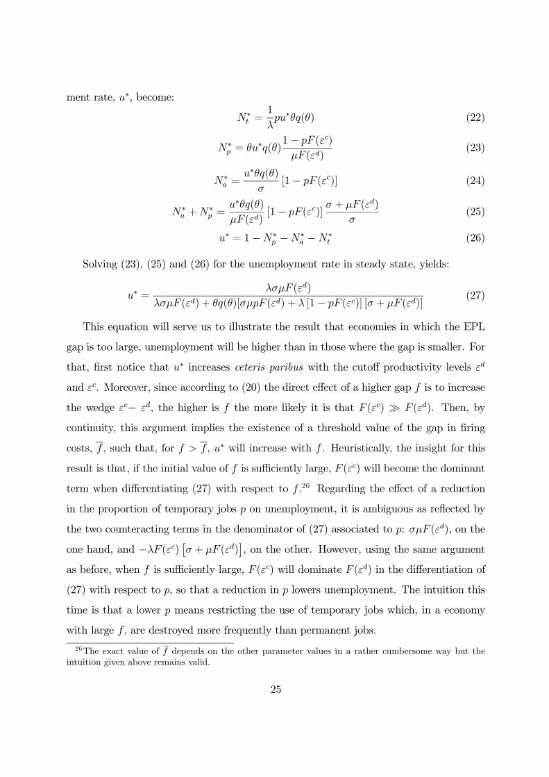
λσμF (εd) + θq(θ)[σμpF (εd) + λ [1− pF (εc)] [σ + μF (εd)](27)
This equation will serve us to illustrate the result that economies in which the EPL
gap is too large, unemployment will be higher than in those where the gap is smaller. For
that, first notice that u∗ increases ceteris paribus with the cutoff productivity levels εd
and εc. Moreover, since according to (20) the direct effect of a higher gap f is to increase
the wedge εc− εd, the higher is f the more likely it is that F (εc) À F (εd). Then, by
continuity, this argument implies the existence of a threshold value of the gap in firing
costs, f , such that, for f > f , u∗ will increase with f . Heuristically, the insight for this
result is that, if the initial value of f is sufficiently large, F (εc) will become the dominant
term when differentiating (27) with respect to f .26 Regarding the effect of a reduction
in the proportion of temporary jobs p on unemployment, it is ambiguous as reflected by
the two counteracting terms in the denominator of (27) associated to p: σμF (εd), on the
one hand, and −λF (εc) £σ + μF (εd)¤, on the other. However, using the same argument
as before, when f is sufficiently large, F (εc) will dominate F (εd) in the differentiation of
(27) with respect to p, so that a reduction in p lowers unemployment. The intuition this
time is that a lower p means restricting the use of temporary jobs which, in a economy
with large f , are destroyed more frequently than permanent jobs.
26The exact value of f depends on the other parameter values in a rather cumbersome way but theintuition given above remains valid.
25
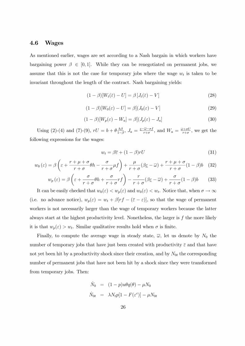
4.6 Wages
As mentioned earlier, wages are set according to a Nash bargain in which workers have
bargaining power β ∈ [0, 1]. While they can be renegotiated on permanent jobs, weassume that this is not the case for temporary jobs where the wage wt is taken to be
invariant throughout the length of the contract. Nash bargaining yields:
(1− β)[Wt(ε)− U ] = β [Jt(ε)− V ] (28)
(1− β)[W0(ε)− U ] = β[(J0(ε)− V ] (29)
(1− β)[Wp(ε)−Wa] = β[(Jp(ε)− Ja] (30)
Using (2)-(4) and (7)-(9), rU = b + θ hβ1−β , Ja =
ε−ω−σfr+σ
, and Wa =ω+σUr+σ
, we get the
following expressions for the wages:
wt = βε+ (1− β)rU (31)
w0 (ε) = β
µε+
r + μ+ σ
r + σθh− σ
r + σμf
¶+
μ
r + σ(βε− ω) +
r + μ+ σ
r + σ(1− β)b (32)
wp (ε) = β
µε+
σ
r + σθh+
σ
r + σrf
¶− r
r + σ(βε− ω) +
σ
r + σ(1− β)b (33)
It can be easily checked that w0(ε) < wp(ε) and w0(ε) < wt. Notice that, when σ→∞(i.e. no advance notice), wp(ε) = wt + β[rf − (ε − ε)], so that the wage of permanent
workers is not necessarily larger than the wage of temporary workers because the latter
always start at the highest productivity level. Nonetheless, the larger is f the more likely
it is that wp(ε) > wt. Similar qualitative results hold when σ is finite.
Finally, to compute the average wage in steady state, ω, let us denote by N0 the
number of temporary jobs that have just been created with productivity ε and that have
not yet been hit by a productivity shock since their creation, and byN0t the corresponding
number of permanent jobs that have not been hit by a shock since they were transformed
from temporary jobs. Then:
N0 = (1− p)uθq(θ)− μN0
N0t = λNtp[1− F (εc)]− μN0t
26

such that their steady-state values become:
N0 =(1− p)uθq(θ)
μ
N0t =puθq(θ)[1− F (εc)]
μ
Using the previous employment sizes, it follows that the weighted average wage in this
economy becomes:
ω =Ntwt +
N0t1−F (εc)
R ε
εcw0(x)dF (x) +N0w0(ε) +
(Np−N0t−N0)1−F (εd)
R ε
εdwp(x)dF (x)
1− u−Na (34)
For example, assuming that F (.) is the c.d.f. of a uniform distribution U [ε, ε] and that
there is no advance notice, ω is given by:
ω =βhθ(1− u) + β ε (Nt +N0) + β ε+εc
2Not + β ε+εd
2(Np −N0 −N0t)
(1− u) (1− b(1− β)) + f(μ+ r)(N0 +Not)− frNp (35)
5 Accounting for the impact of the crisis
In this section, we first show how we calibrate a number of key parameters in the model
and then discuss the results of a simulation exercise where we try to ascertain the extent
to which the difference in EPL regulation between Spain and France can account for the
strikingly different evolution of their respective unemployment rates during the crisis.
5.1 Calibration of the model
The length of a model period is chosen to be one quarter. Some of the values of the
model’s parameters can be imputed directly from data, but others need to be endogenously
calibrated to fit a set of labor market magnitudes. Our reference period for the calibration
is the latter part of the boom preceding the recession, namely 2005:1-2007:4. The reason
is that the unemployment rates in both countries were similar at that time and our goal
is precisely to let the model explain the unemployment rate in the bad state (after the
crisis) relative to the good state (before the crisis).
Parameter values are presented in Table 2. The interest rate r is set at 1% per quarter.
As in most of the literature (see, e.g., Petrongolo and Pissarides, 2001), we set the value
27

for both the elasticity of the matching function with respect to unemployment (α) and
bargaining power (β) equal to 0.5.
As for the unemployment benefit indicator b, we use statutory replacement rates cor-
rected for benefit coverage, setting it to 55% for France and 58% for Spain. Indicators
f , σ, and p are chosen to represent each country’s EPL. As regards f , recall that it
reflects red-tape firing costs. Kramarz and Michaud (2010) calculate the average firing
cost for permanent workers in France to be around one year’s wages, with red-tape costs
accounting for one third of this amount (i.e. 1.33 quarters). For Spain, we compute it as
the (weighted) difference between actually paid severance (45 days of wages per year of
service, in either individual or collective dismissals), which is induced by labor courts and
authorities, and statutory severance for dismissals based on economic reasons (20 days).
Making use of observed employment tenures yields a value of 2 quarters. Thus, the value
of f for Spain is 50% higher than in France. In contrast, the average advance notice
period (1/σ) is longer in France, where it is set to last four months (σ = 0.75), than in
Spain, where it is set at 3 weeks (σ = 4.3).27
Parameter p, which represents the proportion of newly created contracts that are
temporary, is set to 0.85 in France and 0.91 in Spain in the boom. As already indicated,
one of the main reasons for the larger value of p in Spain is the much higher weight of
employment in the construction industry during the reference period which, as argued
before, has been an important source of hiring of temporary workers in this country.
Parameter λ, which captures the (inverse of) the duration of temporary contracts, is set
equal to 0.88 both in France and Spain before the crisis, in line with the information
drawn from their Labor Force Survey (LFS).28
To simplify computations, the idiosyncratic productivity shock is assumed to be uni-
formly distributed, with ε = 0 and ε = 1. Finally, to uncover the values of the remaining
27In France, the advance notice period is 2 months but it increases to 3 months in many collectiveagreements and above 6 months for collective layoffs. Further, the fact that employers ought to interviewthe worker often implies that it takes around one more month before the employer can send the letterletting the worker know that he/she is fired. In Spain, Law 45/2002 , discussed in Section 3.1, has reducedsubstantially the advance notice period since 2002.28For Spain we also use Social Security data, namely the Muestra Continua de Vidas Laborales (MCVL).
28

three parameters (h, m0, and μ), for which no direct information is available, we calibrate
them to match the outcomes of the following three equations defining key labor market
variables (targets) related to temporary and permanent employment jobs and the overall
unemployment rate in each economy, which are computed using the French and Spanish
LFS. The first equation refers to the destruction rate of permanent jobs, which is defined
(in steady state) by:σN∗
f
N∗p +N
∗a
=σμF (εd)
σ + μF (εd)(36)
Secondly, we use the share of temporary jobs in the total stock of jobs (in steady
state), given by:
N∗t
N∗t +N
∗p +N
∗a
=pσμF (εd)
λ [σ + μF (εd)] [1− pF (εc)] + pσμF (εd) (37)
Lastly, we use the steady-state unemployment rate given in equation (27).
Once the model has been calibrated to reproduce the stylized facts during the reference
period, we obtain simulations for the recession allowing for adverse changes in the pro-
ductivity distribution and possibly in mismatch. These simulations are obtained for two
specifications of the average wage ω applied to compute the monetary flows of the firing
cost and the unemployment benefit during the recession. In the first one we consider that
ω corresponds to the contemporaneous calibrated average wage (i.e. in the bad state). In
the second specification ω takes its previously calibrated value in the good state. This is
meant to mimic the fact in reality unemployment benefits and severance pay are linked to
workers’ previous experience and tenure, respectively. For notational convenience, these
two specifications will be labeled as the endogenous wage model and the fixed f— b model
respectively.
5.2 Simulation results
In this section we summarize the main results of several simulation exercises. We present
targets (actual data) and outcomes (simulated data) for both countries in the expansionary
and recessionary periods, using the two alternative ways of computing ω just described.
29

For the sake of brevity, however, we will mainly focus on the results stemming from the
fixed f— b model, which we see as a more realistic setup.
Table 3 presents the data (target values) and the steady-state value of the unem-
ployment rate and temporary contract share during the expansion (based on data for
2005:1-2007:4) and the recession (2008:1-2009:4).29 As can be observed, for the reference
expansionary period, for both countries we are able to match fairly well the chosen target
variables, especially the unemployment and the temporary employment rates.
We follow two approaches in running the simulations for the recession. First, we
consider a baseline simulation where the only degree of freedom in matching targets during
the slump is a parameter controling the severity of the productivity shock through a shift
in its distribution, whereas all other parameters in the model remain the same as in the
preceding expansion. Specifically, we assume that the productivity distribution is shifted
by a multiplicative factor γ, so that productivity is assumed to be uniformly distributed
with support γ[ε, ε] and γ is calibrated to match the required three targets during the
recession. Secondly, we compute an alternative simulation where, besides the severity of
the shock, we allow for another model parameter to change, namely, m0. This is meant
to allow reallocation shocks to play a role in capturing, e.g., mismatch created by the
collapse of the construction industry in Spain, so as to check if there is any improvement
in the overall matching of the targets.
Table 3 (row 4), shows that the baseline simulation allows us to match fairly well
the unemployment and temporary employment rates for France during the recession with
a value of γ equal to 0.90, namely and adverse shift of 10% in average productivity.
Notice, however, that this exercise makes sense only if the unemployment rate reaches its
steady state value fast enough. Figure 6 shows that this is indeed the case: the speed
of adjustment of the unemployment rate is high in France. Most of the adjustment to
the new steady state after the negative shock at the origin of the recession is made in 6
29Given the trending behavior of the unemployment and the temporary employment rates, especiallyin Spain, in a few instances we have replaced the period average by a given data point which we see asmore representative of the corresponding business cycle.phase.
30

months (25 weeks).30
Table 3 (row 8), shows that the baseline simulation for Spain with γ = 0.77 —i.e. a
much more adverse shock than in France— matches the value of the unemployment rate
during the recession well but it fails badly in matching the share of temporary jobs, which
has fallen from 33.3% to 27% whereas the simulation yields an increase to almost 38%.
Given this unsatisfactory result and the arguments posed in Section 3.4 about the likely
increase in mismatch following the negative aggregate shock in Spain, we perform the
alternative simulation where we allow for a newly calibrated value of m0 together with a
new γ. This calibration exercise yields an increase in the degree of mismatch, captured
by a reduction of m0 from its initial value of 2.5 to 1.5 and a similar value for γ to that
obtained for France, namely γ = 0.87. Notice that the outward shift in the Beveridge
curve illustrated in Figure 2 reflects reallocation distortions rather than aggregate shocks
and hence the correct interpretation of the recession in Spain would be a combination of
both types of shocks. In line with the discussion in Section 3.4, higher mismatch leads
to a rise in unemployment through lower labor mobility driven both by the higher risk
involved in the increasing destruction of temporary jobs and the rigid regulations affecting
the Spanish rental market. In other words, workers who have lost their jobs in regions
with high unemployment, because of the collapse of the construction industry, find it very
costly to move to other regions where unemployment is lower. The results reported in
the last row of Table 3 for this alternative scenario show a substantial improvement in
matching the target on temporary work (27% in the data vs. 27.9% in the simulation),
while the much higher unemployment rate remains satisfactorily reproduced.
Figure 7 represents the transitional dynamics of the unemployment rate for Spain.
As in France, it turns out that the speed of adjustment to the steady state is very fast.
Accordingly, comparing steady states in the expansion and the recession allows us to
30The dynamics are easy to compute because the core of the model is forward looking. As soon as theeconomy is hit by an unfavorable shift in the distribution of productivity, the thresholds jump to theirnew stady-state values. We then essentially look at the adjustment of the stocks given the new flows,noting that some permanent workers will be laid off even without having been hit by an “idiosyncratic”shock because of the shift in the thresholds.
31

account well for changes in the unemployment rates in both countries.
5.2.1 Counterfactual simulations: Spain with French EPL regulations
Once we have managed to get a calibration that behaves well in both the good and bad
states, we can use this model to run counterfactual simulations aimed at gauging the share
of the increase in unemployment induced by the recession in Spain that can be attributed
to differences in its EPL vis-à-vis France’s. In other words, we carry out this counterfactual
simulation by computing what would have been the increase in unemployment during the
Great Recession had Spain adopted French EPL just before the slump started.31
We interpret the adoption of French EPL in two ways, namely in a broad and in a
narrow sense. First, it is interpreted as involving not only the direct effect on worker
turnover of adopting a lower value of f but also the related indirect effects of a reduction
in f on the use of temporary contracts. A lower f is bound to lead to many more
conversions as well as more direct hiring of workers under permanent contracts. Thus,
under this broad interpretation, besides using the French value of f , we also impute to
Spain the French share of hires on temporary jobs, p. This can also be interpreted as a
tightening of the enforcement of the criteria for allowing the use of temporary contracts.
The results from these simulations are presented in Table 4. To compute the coun-
terfactual rise in Spanish unemployment, we follow a difference-in-differences approach
where we compare steady-state unemployment before and after the negative aggregate
shock in France and in Spain. For instance, for the fixed f— b model under the broad
interpretation of EPL, the first row in panel A of Table 4 shows the result of subtracting
from the overall change in unemployment, 7.43 pp., the change predicted had Spain had
the French parameters, namely, 4.05 pp. The implication is that the recession would have
raised the unemployment rate in Spain by 3.38 pp. less (i.e. about 45% of the actual
increase) had Spain adopted French EPL rather than kept its own. The endogenous wage
model provides a lower outcome of 1.42 pp. (about 20% less unemployment than the
31Notice that this assumption about the timing of the adoption of French EPL in Spain implies thatwe do not need to re-calibrate the model in the good state.
32

actual increase) revealing that higher wage flexibility reduces the adverse effects of the
EPL gap and the corresponding widespread use of temporary contracts on unemployment.
However, it is likely that the endogenous wage model overestimates downward wage flex-
ibility since, according to the simulations for this case real wages fall by 0.2%, while in
reality they increased by 2.5% during the slump (see Table 1).
Regarding the dynamics, Figure 8 depicts three transition paths of the Spanish un-
employment rate in the recession for the fixed f— b model. Instead of depicting the
unemployment rate in levels, we plot the deviations of the unemployment rate following
the recession from the steady-state value in the good state, i.e. u = 10.2% (see the third
panel in Table 3). The solid line corresponds to the simulation with Spanish parameters
whereas the dashed line captures the case where the values of f and p are replaced by the
French ones. As can be observed, the dynamics in the counterfactual scenario exhibit an
overshooting of about 2 pp. in the short-run after the adverse productivity shock hits the
economy. The reason is that a reduction in the EPL gap, concerning both firing costs and
the use of temporary contracts, exacerbates job destruction in the short run during the
recession by making layoffs less expensive. Specifically, an increase in the productivity
cutoff for job destruction, εd, from 0.76 to 0.86 induces the overshooting. However, in the
long run, this is offset by much higher job creation, so that unemployment goes down to
a new steady state with the properties discussed above: i.e. about 3.4 pp. larger when
Spain keeps its own EPL rather than having adopted the French one.
Next, panel B in Table 4 presents the results of the simulation under the narrow
interpretation of French EPL adoption, i.e. Spanish unemployment with French layoff
costs but the Spanish regulation of temporary jobs. The line with crosses of Figure 8
depicts the transitional dynamics of the unemployment rate in this case. The result of
the counterfactual increase in Spanish unemployment, is quite smaller than before. This
result stresses the importance of the regulation of fixed temporary jobs in combination
with a reduction in the EPL gap, especially because, as stressed in Section 3.4, we believe
that there should be a close link among changes in f and in p. Endogeneizing p as a
33

function of f is bound to be hard in this type of equilibrium search and matching models
but it remains a relevant item in our research agenda.
Finally, panel C in Table 4 reports the results obtained in the converse simulation
exercise, now addressing the question: By how much would French unemployment have
risen during the recession had France adopted Spanish EPL? In line with our previous
discussion, we use the broad interpretation of Spanish EPL in terms of the bundle of
parameters (f, p). The result is that, instead of the observed rise of 1.5 pp., the French
unemployment rate would have risen by 3.1 pp., that is 1.9 pp. more than with their own
regulations when the average wage ω applied to f and b remains as in the good state,
and by only 1.3 pp. under the endogenous wage model. Therefore, these result confirm
the previous counterfactual findings for Spain that a higher (f, p) combination induces a
larger increase in unemployment to a given negative shock.
6 Conclusions
In this paper we explore how much of the significantly larger increase in unemployment
in Spain vis-à-vis France during the ongoing recession can be accounted for the difference
in EPL between the two countries. We have argued that the larger gap between the
dismissal costs of workers with permanent and temporary contracts in Spain as compared
to France has led to different labor mobility and industrial specialization, huge flows of
temporary workers into and out of unemployment and, as a result, large job losses during
the Great Recession.
To carry out this task, inspired by previous work by Blanchard and Landier (2002)
and Cahuc and Postel-Vinay (2002), we have used a search and matching model that
extends Mortensen-Pissarides (1994) to allow for the distinction between temporary and
permanent jobs entailing different dismissal costs. After calibrating the parameters with
data for the two economies, we simulate the model to replicate a few key labor market
magnitudes for the expansion (2005-2007) and recession periods (2008-2009).
Subsequently we undertake several counterfactual exercises involving the key parame-
34
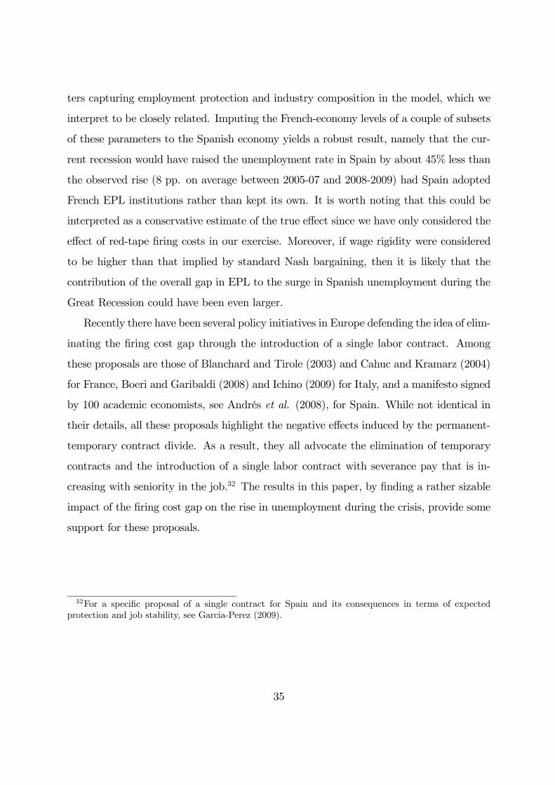
ters capturing employment protection and industry composition in the model, which we
interpret to be closely related. Imputing the French-economy levels of a couple of subsets
of these parameters to the Spanish economy yields a robust result, namely that the cur-
rent recession would have raised the unemployment rate in Spain by about 45% less than
the observed rise (8 pp. on average between 2005-07 and 2008-2009) had Spain adopted
French EPL institutions rather than kept its own. It is worth noting that this could be
interpreted as a conservative estimate of the true effect since we have only considered the
effect of red-tape firing costs in our exercise. Moreover, if wage rigidity were considered
to be higher than that implied by standard Nash bargaining, then it is likely that the
contribution of the overall gap in EPL to the surge in Spanish unemployment during the
Great Recession could have been even larger.
Recently there have been several policy initiatives in Europe defending the idea of elim-
inating the firing cost gap through the introduction of a single labor contract. Among
these proposals are those of Blanchard and Tirole (2003) and Cahuc and Kramarz (2004)
for France, Boeri and Garibaldi (2008) and Ichino (2009) for Italy, and a manifesto signed
by 100 academic economists, see Andrés et al. (2008), for Spain. While not identical in
their details, all these proposals highlight the negative effects induced by the permanent-
temporary contract divide. As a result, they all advocate the elimination of temporary
contracts and the introduction of a single labor contract with severance pay that is in-
creasing with seniority in the job.32 The results in this paper, by finding a rather sizable
impact of the firing cost gap on the rise in unemployment during the crisis, provide some
support for these proposals.
32For a specific proposal of a single contract for Spain and its consequences in terms of expectedprotection and job stability, see Garcia-Perez (2009).
35

Appendix
Table A1. Employment protection legislation in France and Spain
Permanent contracts Temporary contracts
France
* Notice period 1 month if 6<seniority (months)< 242 months if seniority (months) 24
* Severance pay1. Economic 6 days of wages pys. (20% of wage) 3 days of wages pys.reasons +0.08 days’ wages pys.>10 yrs
(1/15 of monthly wage)2. Personal Minimum seniority: 1 yearreasons 3 days of wages pys. (10% of wage)
(before July 2008) +0.04 days’ wages pys.>10 yrs
Observations Personalized plan Max. duration: 24 monthsfor up to 12 months Restricted to 9 cases
(see text)
Spain
* Notice period 1 month
* Severance pay1. Economic 20 days of wages pys. 8 days of wages pys.reasons Max. seniority coverage: 12 months (0 days in some cases,
see text)
Observations Collective dismissal requires Max. duration: 24 monthsadministrative approval Unrestricted
2. Unfair 45 days of wages pys.dismissal Max. seniority coverage: 42 months
Note: “pys.” means per year of service.
36

References
[1] Andrés, J. et al. (2009), “Propuesta para la Reactivación Laboral en España”(2009), El País, 26 April (“A Proposal to Restart the Spanish Labor Market”,crisis09.es/PDF/restart-the-labor-market.pdf).
[2] Antolín, P. and O. Bover (1997), “Regional Migration in Spain: The Effect of Per-sonal Characteristics and of Unemployment, Wage and House Price Differentials us-ing Pooled Cross-Sections”, Oxford Bulletin of Economics and Statistics 59, 215-235.
[3] Barceló, C. (2006), “Housing Tenure and Labour Mobility: A Comparison acrossEuropean Countries”, Banco de España Working Paper 0603.
[4] Becker, S. O., S. Bentolila, A. Fernandes, and A. Ichino (2010), “Youth Emancipa-tion and Perceived Job Insecurity of Parents and Children”, Journal of PopulationEconomics 23, 1047-1071.
[5] Bentolila, S. and J. J. Dolado (1991), “Mismatch and internal migration in Spain,1962-1986”, in F. Padoa Schioppa (ed.), Mismatch and labour mobility, CambridgeUniversity Press, Cambridge.
[6] Bentolila, S., J. J. Dolado, and J. F. Jimeno (2008a), “Does Immigration affect thePhillips Curve? Some Evidence for Spain”, European Economic Review 52, 1398-1423.
[7] Bentolila, S., J. J. Dolado, and J. F. Jimeno (2008b), “Two-tier Employment Pro-tection Reforms: The Spanish Experience”, CESifo DICE Report 4/2008.
[8] Bentolila, S. and A. Ichino (2008), “Unemployment and Consumption Near and FarAway from the Mediterranean”, Journal of Population Economics 21, 255-280.
[9] Bentolila, S. and J. F. Jimeno (2006), “Spanish Unemployment: The End of the WildRide?”, in M. Werding (ed.), Structural Unemployment in Western Europe. Reasonsand Remedies, MIT Press, Cambridge, MA.
[10] Bentolila, S. and G. Saint-Paul (1992), “The Macroeconomic Impact of FlexibleLabor Contracts, with an Application to Spain”, European Economic Review 36,1013-1047.
[11] Blanchard, O. J. and A. Landier (2002), “The Perverse Effects of Partial LaborMarket Reform: Fixed Duration Contracts in France”, Economic Journal 112, 214-244.
37

[12] Blanchard, O. J. and J. Tirole (2003), “Contours of Employment Protection Reform”,MIT Department of Economics Working Paper 03-35.
[13] Boeri T. and P. Garibaldi P. (2007), “Two Tier Reforms of Employment ProtectionLegislation. A Honeymoon Effect?”, Economic Journal 117, F357-F385.
[14] Boeri T. and P. Garibaldi P. (2008), Un Nuovo Contratto per Tutti, Chiarelettere,Torino.
[15] Bouvet, F. (2009), “The Beveridge Curve in Europe: New Evidence using Nationaland Regional Data”, mimeo, Sonoma State University.
[16] Cahuc, P. and S. Carcillo (2006), “The Shortcomings of a Partial Release of Employ-ment Protection Laws: The Case of the 2005 French Reform”, IMF Working Paper06/301.
[17] Cahuc. P. and F. Kramarz (2004), De la précarité à la mobilité, vers une sécuritésociale professionnelle, Rapport pour le Ministre de l’Economie et des Finances,La documentation Française, available at ladocumentationfrancaise.fr/rapports-publics/054000092/index.shtml
[18] Cahuc, P. and F. Postel-Vinay (2002), “Temporary Jobs, Employment Protectionand Labor Market Performance”, Labor Economics 9, 63-91.
[19] Cahuc, P., F. Postel-Vinay and J. M. Robin (2006), “Wage Bargaining with On-The-Job Search: A Structural Econometric Model”, Econometrica 74, 323-64.
[20] Costain, J., Juan F. Jimeno and Carlos Thomas (2010), “Employment Fluctutationsin a Dual Labor Market”, Banco de España, Working Paper 1013.
[21] Eurostat (2009), Youth in Europe, Publications Office of the European Union, Lux-embourg.
[22] Garcia-Perez, J. I. (2009), “¿Qué Efectos Tendría un Contrato Único sobrela Protección del Empleo?”, in J. Dolado and F. Felgueroso (eds.), Prop-uesta de Reactivación Laboral en España, Fedea, Madrid, available at cri-sis09.es/ebook_propuesta_laboral/Propuesta_reactivacion_laboral_art_6.pdf
[23] Garcia-Perez, J. I. and Y. F. Rebollo-Sanz (2009), “Do Wage Subsidies Affect theSubsequent Employment Stability of PermanentWorkers?: The Case of Spain”,Mon-eda y Crédito 228, 65-102.
[24] Garibaldi, P. (1998), “Job Flow Dynamics and Firing Restrictions”, European Eco-nomic Review 42, 245-75.
38

[25] Ichino, A. and Riphahn, R. (2005), “The Effect of Employment Protection onWorkerEffort - A Comparison of Absenteeism During and After Probation”, Journal of theEuropean Economic Association 3, 120-143.
[26] Ichino, P. et al. (2009), “Disegno di Legge per la Transizione a un Regime di Flexi-curity, n. 1481”, 25 March. Synthesis in English at pietroichino.it/?p=3536.
[27] Kramarz, F. and M. L. Michaud (2010), “The Shape of Hiring and Separation Costs”,Labour Economics 17, 27-37.
[28] Kramarz, F. and T. Philippon (2001), “The Impact of Differential Payroll Tax Sub-sidies on Minimum Wage Employment”, Journal of Public Economics 82, 115-146.
[29] Layard, R., S. Nickell, and R. Jackman (1991), Unemployment. Macroeconomic Per-formance and the Labor Market, Oxford University Press, Oxford.
[30] Lazear, E.(1990), “Job Security Provisions and Employment”, Quarterly Journal ofEconomics, 105, 699-726.
[31] L’Haridon, O. and F. Malherbet (2009), “Employment Protection Reform in SearchEconomies”, European Economic Review 53, 255-273.
[32] Ljungqvist, L. (2002), “How Do Layoff Costs Affect Employment?”, Economic Jour-nal 112, 2002, 829-853.
[33] Lopez-Garcia, M. A. (2004), “Housing, Prices and Tax Policy in Spain”, SpanishEconomic Review 6, 29-52.
[34] Malcomson, J. M. (1999), “Individual Employment Contracts”, in O. Ashenfelterand D. Card (eds.), Handbook of Labor Economics, ch. 35, 2291-2372.
[35] Mortensen, D. T. and C. A. Pissarides (1994), “Job Creation and Job Destructionin the Theory of Unemployment”, Review of Economic Studies 61, 397-415.
[36] Organisation for Economic Cooperation and Development (OECD) (2004), Employ-ment Outlook, OECD, Paris.
[37] OECD (2005), Employment Outlook, OECD, Paris.
[38] Oswald, A. J. (1999), “The Housing Market and Europe’s Unemployment: A Non-Technical Paper”, mimeo, University of Warwick.
[39] Petrongolo, B. and C. A. Pissarides (2001), “Looking into the Black Box: A Surveyof Matching Functions”, Journal of Economic Literature 39, 390-431.
39

[40] Pissarides, C. A. (2000), Equilibrium Unemployment Theory, 2nd ed., The MIT Press,Cambridge, MA.
[41] Rupert, P. and E. Wasmer (2009), “Housing and the Labor Market: Time to Moveand Aggregate Unemployment”, mimeo, Sciences-Po, Paris.
[42] Saint-Paul, G. (1996), Dual Labor Markets, The MIT Press, Cambridge, MA.
[43] Saint-Paul, G. (1997),“Is Labour Rigidity Harming Europe’s Competitiveness? TheEffect of Job Protection on the Pattern of Trade and Welfare”, European EconomicReview 41, 499-506.
[44] Saint-Paul, G. (2000), The Political Economy of Labour Market Institutions, OxfordUniversity Press, Oxford.
[45] Sala, H., J. I. Silva, and M. E. Toledo (2009),“Flexibility at the Mar-gin and Labor Market Volatility in OECD Countries”, SSRN, available at:ssrn.com/abstract=1377909.
[46] Vandenbrande et al. (2006), Mobility in Europe, Office for Official Publications of theEuropean Union, Luxembourg.
[47] Visser, J. (2009), “ICTWSS: Database on Institutional Characteristics of TradeUnions, Wage Setting, State Intervention and Social Pacts in 34 countries between1960 and 2007”, Amsterdam Institute for Advanced Studies (www.uva-aias.net/208).
[48] Wasmer, E. (1999), “Competition for Jobs in a Growing Economy and the Emergenceof Dualism in Employment”, Economic Journal 109, 349-371.
40

05
1015
20
1975q1 1980q1 1985q1 1990q1 1995q1 2000q1 2005q1 2010q1quarter
France Spain
Figure 1: Unemployment rate in France and Spain, 1976-2010
41

Table 1: Labor market evolutions in France and Spain
Levels (%) 1998:1 2007:4 2009:4
1. Unemployment France 10.3 7.5 9.7Spain 15.2 8.7 18.9
2. Fixed-term employment1 France 13.8 14.3 13.1Spain 33.3 30.9 25.1
3. Hours of work2 France 40.7 37.7 37.4Spain 38.8 39.0 39.1
Annual growth rates (%)3 1998:1-2007:4 2008:1-2009:4
4. Gross Domestic Product France 2.3 -1.1Spain 3.7 -2.2
5. Labor force France 0.8 0.9Spain 3.3 1.3
6. Employment France 1.1 -0.3Spain 4.2 -4.6
7. Private non-agricultural employees:(a) Total France 1.5 -1.6
Spain 5.6 -5.7(b) Construction France 2.4 -1.8
Spain 8.1 -19.8(c) Manufacturing France -0.7 -3.2
Spain 2.0 -10.8(d) Market services France 2.2 -1.1
Spain 6.8 -0.98. Real hourly earnings4 France 1.3 1.1
Spain 0.3 2.59. Hiring on temporary contracts5 France 78.6 83.3
Spain 90.5 89.6
Notes: 1 As a share of employees. 2 Full-time employees. 3 Computed as annual rates of end-of-period on start-of period quarterly levels. 4 Deflated by GDP Deflator, seasonally adjusted.5 Average share over the corresponding period.Sources: (1),(4)-(6), OECD Economic Outlook Database (www.oecd.org); (2),(3) Euro-stat Statistics Database (epp.eurostat.ec.europa.eu); (7), INSEE BDM Macroeconomic Data-base (www.bdm.insee.fr) for France and INE, Encuesta de Población Activa (www.ine.es)for Spain; (8) OECD Main Economic Indicators Database (www.oecd.org), (9) ACOSS(www.acoss.urssaf.fr) for France and Ministerio de Trabajo e Inmigración, Boletín de Estadísti-cas Laborales (www.mtin.es).
42

Figure 2: Beverigde curve for Spain
43

Figure 3: Labor market equilibrium
44

Figure 4: Effects of an increase in the firing cost (f)
45

Figure 5: Effects of a reduction in the proportion hires on temporary contracts (p)
46

Table 2: Calibrated and estimated parameters1
France Spain
Standard parameters:Interest rate r 0.01 0.01Matching function elasticity α 0.50 0.50Worker bargaining power β 0.50 0.50
Institutional parameters:Unemployment benefit replacemente rate b 0.55 0.58Severance pay for permanent employees f 1.33 2.00
Dual labor market flow rates:Probability of hiring into a temporary job p 0.85 0.91Probability of temporary contract ending λ 0.88 0.88
Parameters estimated by indirect inference:Cost of keeping jobs vacant h 0.50 0.25Matching efficiency level in expansion m0 1.50 2.50Matching efficiency level in recession m0
0 1.50 1.50Incidence rate of productivity shocks μ 0.04 0.09Lower bound of productivity shock ε 0.00 0.00Shocks multiplicative shift factor in recession γ 0.90 0.87Advance notice rate σ 0.75 4.30
1 Reference period: 2005:1-2007:4.
47

Table 3: Simulation results
Unemployment Perm. jobs Temporaryrate destruction employment
rate rate
France - Expansion1. Data 0.0860 0.0150 0.12602. Model 0.0854 0.0305 0.1137
France - Recession3. Data 0.0980 0.0130 0.12504. Model 0.0973 0.0304 0.1145
Spain - Expansion5. Data 0.1020 0.0470 0.33306. Model 0.1022 0.0655 0.3300
Spain - Recession7. Data 0.1790 0.0400 0.27008. Baseline 0.1736 0.0641 0.37939. Alternative 0.1765 0.0611 0.2796
48

Table 4: Differential increase in unemployment in Spain induced by the recession explainedby differences with France in the alternative simulation (percentage points)
∆uSP ∆uSP (FR) ∆uSP—∆uSP (FR)
A. Spain with French EPL: f and p* Fixed f − b model 7.43 4.05 3.38* Endogenous wage model 7.27 5.85 1.42
B. Spain with French EPL: f* Fixed f − b model 7.43 6.13 1.30* Endogenous wage model 7.27 7.28 -0.01
∆uFR ∆uFR(SP ) ∆uFR—∆uFR(SP )
C. France with Spanish EPL: f and p* Fixed f − b model 1.19 3.08 -1.90* Endogenous wage model 1.28 2.58 -1.30
Note: ∆uSP denotes the change in unemployment explained by the model simulatedfor the Spanish economy and ∆uSP (FR) the change in unemployment explained by themodel simulated for the Spanish economy with the indicated set of parameter valuescorresponding to the simulated French economy. The mirror definitions apply to ∆uFRand ∆uFR(SP ).
49
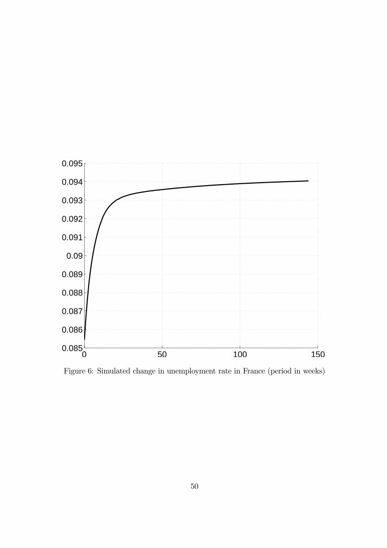
0 50 100 1500.085
0.086
0.087
0.088
0.089
0.09
0.091
0.092
0.093
0.094
0.095
Figure 6: Simulated change in unemployment rate in France (period in weeks)
50

0 50 100 1500.1
0.11
0.12
0.13
0.14
0.15
0.16
0.17
0.18
Figure 7: Simulated change in unemployment rate in Spain (period in weeks)
51

0 50 100 1500
0.01
0.02
0.03
0.04
0.05
0.06
0.07
0.08
Figure 8: Change in unemployment rate in Spain with Spanish EPL (solid line), withFrench layoff costs and French regulation of temporary jobs (dotted line), with Frenchlayoff costs and Spanish regulation of temporary jobs (line with crosses), (period in weeks)
52