uncertainty evaluation through ranking of … · 2011-06-08 · uncertainty evaluation through...
TRANSCRIPT

UNCERTAINTY EVALUATION THROUGH RANKING OF SIMULATION MODELS FOR BOZOVA OIL FIELD
A THESIS SUBMITTED TO THE GRADUATE SCHOOL OF NATURAL AND APPLIED SCIENCES
OF MIDDLE EAST TECHNICAL UNIVERSITY
BY
MELEK MEHLİKA TONGA
IN PARTIAL FULFILLMENT OF THE REQUIREMENTS FOR
THE DEGREE OF MASTER OF SCIENCE IN
PETROLEUM AND NATURAL GAS ENGINEERING
MAY 2011

ii
Approval of the thesis:
UNCERTAINTY EVALUATION THROUGH RANKING OF SIMULATION MODELS FOR BOZOVA OIL FIELD
submitted by MELEK MEHLİKA TONGA in partial fulfillment of the require-ments for the degree of Master of Science in Petroleum and Natural Gas Engineering Department, Middle East Technical University by,
Prof. Dr. Canan Özgen _____________________ Dean, Graduate School of Natural and Applied Sciences
Prof. Dr. Mahmut Parlaktuna _____________________ Head of Department, Petroleum and Natural Gas Engineering
Prof. Dr. Serhat Akın _____________________ Supervisor, Petroleum and Natural Gas Engineering Dept., METU
Examining Committee Members:
Prof. Dr. Mahmut Parlaktuna _____________________ Petroleum and Natural Gas Engineering Dept., METU
Prof. Dr. Serhat Akın _____________________ Petroleum and Natural Gas Engineering Dept., METU
Prof. Dr. Mustafa V. Kök _____________________ Petroleum and Natural Gas Engineering Dept., METU
Mustafa Yılmaz, M.Sc. _____________________ Deputy Director, Production Department, TPAO
Deniz Yıldırım, M.Sc. _____________________ Chief Engineer, Production Department, TPAO
Date: _____________________

iii
I hereby declare that all information in this document has been obtained and presented in accordance with academic rules and ethical conduct. I also declare that, as required by these rules and conduct, I have fully cited and referenced all material and results that are not original to this work.
Name, Last name : Melek Mehlika TONGA
Signature :
iv
ABSTRACT
UNCERTAINTY EVALUATION THROUGH RANKING OF SIMULATION MODELS FOR BOZOVA OIL FIELD
TONGA, Melek Mehlika M.Sc., Department of Petroleum and Natural Gas Engineering
Supervisor: Prof. Dr. Serhat AKIN
May 2011, 100 pages Producing since 1995, Bozova Field is a mature oil field to be re-evaluated. When
evaluating an oil field, the common approach followed in a reservoir simulation
study is: Generating a geological model that is expected to represent the reservoir;
building simulation models by using the most representative dynamic data; and
doing sensitivity analysis around a best case in order to get a history-matched
simulation model. Each step deals with a great variety of uncertainty and changing
one parameter at a time does not comprise the entire uncertainty space. Not only
knowing the impact of uncertainty related to each individual parameter but also their
combined effects can help better understanding of the reservoir and better reservoir
management.
In this study, uncertainties associated only to fluid properties, rock physics functions
and water oil contact (WOC) depth are examined thoroughly. Since sensitivity
analysis around a best case will cover only a part of uncertainty, a full factorial
experimental design technique is used. Without pursuing the goal of a history
matched case, simulation runs are conducted for all possible combinations of: 19 sets
of capillary pressure/relative permeability (Pc/krel) curves taken from special core
analysis (SCAL) data; 2 sets of pressure, volume, temperature (PVT) analysis data;
and 3 sets of WOC depths. As a result, historical production and pressure profiles

v
from 114 (2 x 3 x 19) cases are presented for screening the impact of uncertainty
related to aforementioned parameters in the history matching of Bozova field. The
reservoir simulation models that give the best match with the history data are deter-
mined by the calculation of an objective function; and they are ranked according to
their goodness of fit. It is found that the uncertainty of Pc/krel curves has the highest
impact on the history match values; uncertainty of WOC depth comes next and the
least effect arises from the uncertainty of PVT data. This study constitutes a solid
basis for further studies which is to be done on the selection of the best matched
models for history matching purposes.
Keywords: Uncertainty, Ranking, Simulation Models, Factorial Design, Capillary
Pressure, Relative Permeability, Water Oil Contact
vi
ÖZ
BOZOVA PETROL SAHASI İÇİN YAPILAN SİMÜLASYON MODELLERİNİN BELİRSİZLİK DEĞERLENDİRMESİ VE SIRALAMASI
TONGA, Melek Mehlika Yüksek Lisans, Petrol ve Doğal Gaz Mühendisliği Bölümü
Tez Yöneticisi: Prof. Dr. Serhat AKIN
Mayıs 2011, 100 sayfa Bozova Sahası 1995’ten itibaren üreten ve yeniden değerlendirilmesi yapılacak olan
olgun bir petrol sahasıdır. Bir petrol sahasını değerlendirirken yapılan rezervuar
simülasyonu çalışmasında takip edilen genel yaklaşım şu şekildedir: Rezervuarı
temsil etmesi beklenen bir jeolojik model oluşturmak; rezervuarı en iyi temsil eden
dinamik datayı kullanarak simülasyon modelini kurmak; ve tarihsel çakıştırma
sağlanmış bir simülasyon modeli elde etmek için en iyi senaryo üzerinde duyarlılık
analizi yapmak. Her basamakta çeşitli belirsizliklerle çalışıldığından, her seferinde
bir parametreyi değiştirmek tüm belirsizlik uzayını kapsamaz. Sadece her bir tekil
parametreye ilişkin belirsizliğin etkisi değil, aynı zamanda bu belirsizliklerin bileşik
etkilerinin de bilinmesi, rezervuarı daha iyi anlamaya ve daha iyi rezervuar yöneti-
mine yardımcı olur.
Bu çalışmada, sadece akışkan özellikleri, kayaç fiziği fonksiyonları ve su petrol
kontağına ait belirsizlikler derinlemesine çalışılmıştır. En iyi ihtimal senaryosu
üzerine çalışılan duyarlılık analizi belirsizliğin sadece bir kısmını kapsayacağından,
tam faktöriyel deneysel tasarım tekniği kullanılmıştır. Tarihsel çakıştırma sağlanmış
bir senaryo oluşturma amacı güdülmeden, özel karot analizlerinden gelen 19 set
kılcal basınç ve göreli geçirgenlik eğrisi; 2 set PVT analizi ve 3 set su petrol kontağı
derinliğiyle oluşabilecek tüm olası kombinasyonlar için simülasyonlar

vii
koşturulmuştur. Sonuç olarak, sözkonusu parametrelere ait belirsizliklerin Bozova
sahası tarihsel çakıştırması üzerindeki etkisini göstermek amacıyla 114 (2 x 3 x 19)
simülasyon sonucundan gelen tarihsel üretim ve basınç profilleri sunulmuştur. En iyi
tarihsel çakıştırmayı sağlayan simülasyon modelleri bir amaç fonksiyon
hesaplamasıyla belirlenmiş ve simülasyon modelleri uyum iyiliklerine göre
sıralanmıştır. Tarihsel çakıştırma değerleri üzerinde en çok etkiye sahip olan
belirsizliğin kılcal basınç/göreli geçirgenlik eğrileri belirsizliği olduğu, su petrol
kontağı derinliğinin bunu takip ettiği ve en az etkinin PVT datası belirsizliğinden
kaynaklandığı bulunmuştur. Bu çalışma, en iyi çakıştırma sağlanmış modeller
üzerinde tarihsel çakıştırma amaçlı yapılacak gelecek çalışmalar için sağlam bir
temel oluşturmaktadır.
Anahtar Kelimeler: Belirsizlik, Simülasyon Modellerinin Sıralaması, Faktöriyel
Tasarım, Kılcal Basınç, Göreli Geçirgenlik, Su Petrol Kontağı

viii
To Schrödinger’s cat

ix
ACKNOWLEDGEMENTS
I am sincerely grateful to my supervisor Prof. Dr. Serhat Akın for his valuable
suggestions, guidance and support. He has always been accessible and willing to
help throughout my work.
I would like to thank related TPAO authorities for allowing me to use the data of
Bozova Field which enabled me to complete this study. I also offer my regards to
TPAO Production Department Management for their understanding and considera-
tion during my thesis-writing period.
I want to express my thanks to those who worked on developing the geological
model of this study; in particular, Melike Özkaya Türkmen for her cooperation,
valuable time and precious effort, Ceyda Çetinkaya for her contribution and Yıldız
Karakeçe for her substantial guidance throughout the geological modeling process.
Moreover, I wish to thank Murat Demir, Sertuğ Evin, Volkan Üstün, Demet
Çelebioğlu and Deniz Yıldırım; the time we spent together has always been a great
business experience for me through the years at TPAO. My thanks also go to Fatih
Tuğan for encouraging me at the very beginning of this study, and Erkin Gözel for
his kind company on working till late hours at the office.
On a personal note, I am heartily thankful to my fiancé Evren, my brother Alper and
his joyful wife Neşe, and my parents for their patience, understanding and caring
support which has been my source of strength and inspiration. As a result, this tough
period became smooth and rewarding for me.
Last but not the least, I want to offer my special thanks to my sisters Feyza, Güneş
and Sıla, whose existence and love I feel right beside me all the time, wherever they
are. I wish to thank Özlem, Beyza, Demet and Deniz who have always been there for
me with their constant moral support, enthusiasm and motivation whenever I need.
Having such gorgeous friends, I have always considered myself lucky; they are the
true blessings of my life.

x
TABLE OF CONTENTS
ABSTRACT ................................................................................................................ iv
ÖZ ............................................................................................................................... vi
ACKNOWLEDGEMENTS ........................................................................................ ix
TABLE OF CONTENTS ............................................................................................. x
NOMENCLATURE ................................................................................................... xii
LIST OF TABLES ................................................................................................... xiii
LIST OF FIGURES .................................................................................................. xiv
CHAPTERS
1. INTRODUCTION................................................................................................ 1
2. LITERATURE REVIEW .................................................................................... 3
2.1 Classification of Uncertainties ....................................................................... 3
2.1.1 The Different Uncertainty Statistical Behaviors ..................................... 4
2.1.2 The Different Parameters Status ............................................................. 4
2.2 The Importance of Dynamic Uncertainty ...................................................... 5
2.3 The Need to Quantify Uncertainty ................................................................. 7
2.4 Uncertainty Quantification Methods .............................................................. 7
3. BOZOVA FIELD OVERVIEW ........................................................................ 10
3.1 General Overview of The Field.................................................................... 10
3.2 Geological Description of the Field ............................................................. 12
3.2.1 Lithological Description of the Reservoir Level ................................... 12
3.2.2 Structural Geology of the Field ............................................................. 13
4. STATEMENT OF THE PROBLEM ................................................................. 14
5. METHOD OF SOLUTION ............................................................................... 15
5.1 Geological Modeling .................................................................................... 15
5.1.1 Data Input, QA/QC ............................................................................... 15
5.1.2 3D Geological Grid and Petrophysical Parameter Modeling ................ 16
5.1.3 STOOIP Calculation from 3D Geological Model ................................. 18
5.2 Basic Reservoir Engineering ........................................................................ 18

xi
5.2.1 Well Test Interpretations ....................................................................... 19
5.2.2 Bottom Hole Pressure (BHP) Measurements ........................................ 21
5.2.3 Determination of Original Reservoir Pressure (Pi) ............................... 21
5.2.4 The Uncertainty of WOC ...................................................................... 24
5.2.5 The Uncertainty in Pc/Krel Curves ....................................................... 27
5.2.6 The Uncertainty in Fluid Properties ...................................................... 29
5.3 Reservoir Simulation .................................................................................... 30
5.3.1 Making Fluid Model ............................................................................. 30
5.3.2 Making Rock Physics Functions ........................................................... 31
5.3.3 Making Aquifer Model ......................................................................... 33
5.3.4 Running the Simulation Models ........................................................... 36
5.4 History Match Analysis ............................................................................... 37
5.5 Two Level (2k) Factorial Design Technique as an Uncertainty
Quantification Method ....................................................................................... 38
6. RESULTS AND DISCUSSIONS ...................................................................... 44
6.1 Screening the Simulation Results ................................................................ 44
6.1.1 Production Rate Results ........................................................................ 44
6.1.2 Cumulative Production Results ............................................................. 49
6.1.3 BHP Results .......................................................................................... 54
6.2 History Match Analysis Results ................................................................... 57
6.2.1 Ranking Cases (Case Comparison) ....................................................... 57
6.2.2 Simulation and History Match Value Results of the 3 Best Cases ....... 63
6.3 Uncertainty Quantification Results .............................................................. 72
6.3.1 Uncertainty Quantification by Using History Match Statistics ............. 72
6.3.2 Uncertainty Quantification by Two Level (2k) Factorial Design
Technique ....................................................................................................... 76
7. CONCLUSIONS ................................................................................................ 79
8. RECOMMENDATIONS ................................................................................... 81
REFERENCES ........................................................................................................... 82
APPENDICES
A. WELL TEST INTERPRETATION RESULTS ................................................ 86
B. BHP MEASUREMENT DETAILS .................................................................. 96
C. EXPERIMENTAL DESIGN TABLE ............................................................. 100

xii
NOMENCLATURE
WOC : Water oil contact
Pc : Capillary pressure
krel : Relative permeability
SCAL : Special core analysis
PVT : Pressure volume temperature
FWL : Free water level
Swir : Irreducible water saturation
Pce : Pore entry pressure
RSM : Response surface methodology
STOOIP : Stock tank oil originally in place
BHP : Bottom hole pressure
Pi : Original reservoir pressure
RMS : Root mean square

xiii
LIST OF TABLES
TABLES
Table 5.1 Bozova DST parameters and the interpretation results .............................. 20
Table 5.2 Pressure values obtained from DSTs and BHP measurements .................. 21
Table 5.3 PVT analysis results of Bozova-1 sample .................................................. 29
Table 5.4 PVT analysis results of Bozova-3 sample .................................................. 30
Table 5.5 The factorial design for fluid modeling ..................................................... 31
Table 5.6 Initial conditions ........................................................................................ 31
Table 5.7 Normalization parameters for combined vector match .............................. 38
Table 5.8 Coded design matrix with results ............................................................... 39
Table 5.9 Design and calculation matrix; and the results (Saxena and Pavelic, 1971)
.................................................................................................................................... 42
Table 6.1 Ranking simulation models according to their match values .................... 62
Table 6.2 The 3 best and the worst matching cases and match values for each well 63
Table 6.3 Tables for calculating the impact of PVT data uncertainty ....................... 73
Table 6.4 Tables for calculating the impact of WOC depth uncertainty ................... 74
Table 6.5 Tables for calculating the impact of Pc/krel curves uncertainty ................ 75
Table 6.6 Impact of PVT, WOC, Pc/krel uncertainty on different vector matches ... 76
Table 6.7 Coded and uncoded factorial design with results ...................................... 77
Table 6.8 Ranking the average effects on STOOIP ................................................... 78
Table B.1 Amerada BHP measurement details (Bozova-1, 3, 8)............................... 96
Table B.2 Spartek BHP measurement details (Bozova-2, 8, 9) ................................. 98
Table C.1 Experimental Design Table ..................................................................... 100

xiv
LIST OF FIGURES
FIGURES
Figure 2.1 Sources of uncertainties in reservoir modeling workflow (Zabalza-
Mezghani, 2004) .......................................................................................................... 3
Figure 2.2 Relationship between a Pc curve and oil accumulation (Holmes, 2002) ... 6
Figure 3.1 Geographical location of Bozova field ..................................................... 11
Figure 3.2 The daily oil production graph of Bozova field ........................................ 11
Figure 3.3 The bubble map the illustrating cumulative production of each well ...... 12
Figure 5.1 Well sections of Bozova field (Log process by Karakeçe, 2009) ............. 15
Figure 5.2 Structure contour map of Bozova field on top of Reservoir Level (adapted
from Sefunç & Ölmez, 2002) ..................................................................................... 16
Figure 5.3 The porosity-permeability plot obtained from core data .......................... 17
Figure 5.4 Porosity distribution model of the 3D grid ............................................... 17
Figure 5.5 Sw distribution model of the 3D grid ....................................................... 18
Figure 5.6 Date vs. pressure plot of pressure values corrected @1455 m ssTVD ..... 22
Figure 5.7 Pressure vs. depth plot of DST and Amerada BHP measurements .......... 23
Figure 5.8 Pressure vs. depth plot for determination of Pi......................................... 24
Figure 5.9 WOC depths studied in uncertainty analysis ............................................ 26
Figure 5.10 Porosity vs. core and DST permeabilities cross-plot for Reservoir Level
.................................................................................................................................... 27
Figure 5.11 Capillary pressure curves for Reservoir Level ....................................... 28
Figure 5.12 Relative permeability curves for Reservoir Level .................................. 28
Figure 5.13 Smoothed relative permeability curves taken from SCAL data ............. 32
Figure 5.14 Smoothed capillary pressure curves taken from SCAL data .................. 32
Figure 5.15 Decline in reservoir pressure during production observed in the field ... 33
Figure 5.16 Test and production graph of Bozova-1 ................................................. 34
Figure 5.17 Test and production graph of Bozova-3 ................................................. 34
Figure 5.18 Test and production graph of Bozova-8 ................................................. 35
Figure 5.19 Test and production graph of Bozova-2 ................................................. 35
Figure 5.20 Aquifer connected to the bottom of Reservoir Level ............................. 36
Figure 5.21 Geometrical representation of the 23 design (adapted from Saxena and
Pavelic, 1971) ............................................................................................................. 40

xv
Figure 5.22 The high and low level planes for variables x1, x2 and x3 (adapted from
Saxena and Pavelic, 1971) ......................................................................................... 41
Figure 5.23 The high and low level planes for calculating the interaction between x1
and x2 (E12) (adapted from Saxena and Pavelic, 1971) .............................................. 41
Figure 6.1 Oil production rates of simulation models (PVT-1: FM1,2,3) ................. 45
Figure 6.2 Oil production rates of simulation models (PVT-3: FM4,5,6) ................. 46
Figure 6.3 Water production rates of simulation models (PVT-1: FM1,2,3) ............ 47
Figure 6.4 Water production rates of simulation models (PVT-3: FM4,5,6) ............ 48
Figure 6.5 Cumulative oil productions of simulation models (PVT-1: FM1,2,3) ..... 50
Figure 6.6 Cumulative oil productions of simulation models (PVT-3: FM4,5,6) ..... 51
Figure 6.7 Cumulative water productions of simulation models (PVT-1: FM1,2,3) . 52
Figure 6.8 Cumulative water productions of simulation models (PVT-3: FM4,5,6) . 53
Figure 6.9 BHP of simulation models (PVT-1: FM1,2,3) ......................................... 55
Figure 6.10 BHP of simulation models (PVT-3: FM4,5,6) ....................................... 56
Figure 6.11 Combined vector match values of simulation models FM-1, 2, 3 .......... 58
Figure 6.12 Combined vector match values of simulation models FM-1, 2, 3 .......... 59
Figure 6.13 Combined vector match values of simulation models FM-4, 5, 6 .......... 60
Figure 6.14 Combined vector match values of simulation models FM-4, 5, 6 .......... 61
Figure 6.15 Simulation results and vector match values of B-1 for the 3 Best Cases64
Figure 6.16 Simulation results and vector match values of B-2 for the 3 Best Cases65
Figure 6.17 Simulation results and vector match values of B-3 for the 3 Best Cases66
Figure 6.18 Simulation results and vector match values of B-8 for the 3 Best Cases67
Figure 6.19 Simulation results and vector match values of B-9 for the 3 Best Cases68
Figure 6.20 Simulation results and vector match values of the field for the 3 Best
Cases .......................................................................................................................... 69
Figure 6.21 Capillary pressure curves emphasizing the 3 best matching curves ....... 70
Figure 6.22 Qualitative vector match map for the best case FM3_9 ......................... 71
Figure 6.23 Geometrical representation of the 23 design ........................................... 77
Figure A.1 Well test interpretation plots of Bozova-1 DST#1 .................................. 86
Figure A.2 Well test interpretation plots of Bozova-1 DST#2 .................................. 87
Figure A.3 Well test interpretation plots of Bozova-2 DST#1 .................................. 88
Figure A.4 Well test interpretation plots of Bozova-2 DST#2 .................................. 89
Figure A.5 Well test interpretation plots of Bozova-3 DST#1 .................................. 90
Figure A.6 Well test interpretation plots of Bozova-4 DST#1 .................................. 91

xvi
Figure A.7 Well test interpretation plots of Bozova-4 DST#2 .................................. 92
Figure A.8 Well test interpretation plots of Bozova-5 DST#1 .................................. 93
Figure A.9 Well test interpretation plots of Bozova-8 DST#1 .................................. 94
Figure A.10 Well test interpretation plots of Bozova-9 DST#1 ................................ 95
Figure B.1 Pressure vs. depth plots of Amerada BHP measurements ....................... 97
Figure B.2 Pressure vs. depth plots of Spartek BHP measurements .......................... 99
1
CHAPTER 1
INTRODUCTION
In the last decades, the high technology has let us to acquire data more easily,
accurately and frequently. The accuracy of evaluation of an oil field depends on how
all of these data is successfully integrated, for instance in complex numerical reser-
voir models. However, the data may contain serious errors starting from its
acquisition step, to its processing, interpretation and integration steps. The complex
numerical model, which is generated by using parameters with significant uncertain-
ties, becomes a model of stacked uncertainties. As a result, the outputs of this
reservoir modeling workflow, for example, fluid in places, reserves, production
profiles, economic evaluation, etc., will be uncertain (Zabalza-Mezghani, 2004).
The Bozova field, which is studied in this thesis, is a producing oil field of TPAO.
There are several reasons why this field is chosen for the study. The first one was the
need to re-evaluate the field for reserve estimation purposes. The second reason was
the ambiguity of WOC depth. For instance, inspite of the fact that there was no water
contact seen in the logs, Bozova-9 started producing 100 % of water 5 months after
its production start up. This situation aroused two questions: Is there a possible
damage in the casings? Or is there a complex flow mechanism in the reservoir that
leads to water production?
Casings are checked with integrity tests showing no indication of damage and
according to logs cement bond was of moderate strength. The possibility of a weak
casing cement bond interconnecting the perforations and an undetermined water
zone was and still is a question subject to this well. It is also useful to mention that
the water produced from Bozova-9 and the formation water of Reservoir Level have
the same salinity value which again supports the idea that WOC is somehow close to
the perforations of Bozova-9. The second question pointed out the importance of
flow functions, such as Pc or krel curves, derived from SCAL data.

2
Under all of these considerations, a geological modeling and simulation study was
deemed crucial in order to understand the reservoir behavior thoroughly.
The objective of this study is to evaluate dynamic reservoir uncertainties on the
simulation modeling of Bozova oil field and ranking of the simulation models
created for uncertainty evaluation. The study covers uncertainties associated only to
fluid properties, rock physics functions and WOC depth. Uncertainty of any other
type is beyond the scope of this thesis.
The uncertainty range of parameters is not determined by parameter sweeps. In order
to reduce the uncertainty range, experimental data is used in this study. The uncer-
tainty of fluid properties is studied through 2 sets of PVT data, samples of which are
taken from wells Bozova-1 and 3. The uncertainty of rock physics functions is
studied through SCAL data obtained from 19 core plugs, which are taken from
Reservoir Level formation of wells Bozova-1, 2 and 3. PVT and SCAL data were
analyzed by TPAO Research Center. The uncertainty of WOC depth is studied
through 3 different values which are considered to be informative on the determina-
tion of the true reservoir description.
In order to address the full range of uncertainty, simulations are run for all possible
combinations of these uncertain parameters and simulation models are ranked
according to their goodness of fit. Ranking schemes for 114 simulation models are
established and compared. The rankings provide an assessment of all possible model
responses.

3
CHAPTER 2
LITERATURE REVIEW
Sources of uncertainties in reservoir engineering are almost infinite and are any-
where within the reservoir modeling workflow. These are static model, upscaling,
fluid flow modeling, production data integration, production scheme development
and economic evaluation as given in Figure 2.1 (Zabalza-Mezghani, et al., 2004).
Figure 2.1 Sources of uncertainties in reservoir modeling workflow (Zabalza-Mezghani, 2004)
2.1 Classification of Uncertainties
The evaluation and optimization of reservoirs require complex models which contain
many uncertainties. Since there is not a unique methodology that can handle all types
of uncertainties, it becomes important to choose the right methodology to take into
account each uncertainty. The methodology is selected according to statistical
behavior and status of uncertainty.

4
2.1.1 The Different Uncertainty Statistical Behaviors
As stated by Zabalza-Mezghani et al. (2004) three different statistical behaviors can
be used to classify the uncertainties:
Deterministic uncertainty corresponds to a parameter which has a continuous uncer-
tainty range. The parameter may vary between a minimum and a maximum value.
This includes, for instance, uncertainty on any average property (average permeabili-
ty, porosity), correlation length for a geostatistical model, upscaling coefficient
between arithmetic and harmonic laws, horizontal well length, etc.
Discrete uncertainty corresponds to a parameter that can take only a finite number of
discrete values. This includes, for instance, an uncertainty on a few possible deposi-
tional scenarios, the Boolean behavior of a fault which is conductive or not, or the
optimal number of new production infill wells to be implemented.
Stochastic uncertainty corresponds to an uncertainty which does not have a smooth
behavior on production responses. For instance, a small incrementation of the
parameter value may lead to completely different results in terms of production
profiles. It also corresponds to an uncertainty that can take infinity of equiprobable
discrete values. For instance, infinity of equiprobable structural maps, fracture maps,
geostatistical realizations, and history matched models, etc.
2.1.2 The Different Parameters Status
As stated by Zabalza-Mezghani et al. (2004) two different uncertainty status can be
used to classify the uncertainties:
Uncontrollable status corresponds to a parameter on which the engineer cannot have
any control. This includes typically any physical parameters inherent to the reservoir
such as petrophysical values, reservoir structure and geology, etc. For such a para-
meter, the uncertainty can partially be reduced through additional data acquisition

5
and history matching process but must still be faced using for instance some sam-
pling methods.
Controllable status corresponds to a parameter for which the value is unknown but
can be controlled, such as a well location, water injection rate, etc.
2.2 The Importance of Dynamic Uncertainty
The uncertainties of the reservoir properties such as the geological and petrophysical
data are very often given more attention than the uncertainties of dynamic reservoir
parameters. Input data, such as fluid properties, Pc/krel curves and WOC depth, are
very important for the dynamic reservoir simulations as they dictate the accuracy of
the simulation prediction. In order to reduce the uncertainty for Pc/krel curves and
PVT data, experimental data is used in this study. On the other hand, it should be
noted that experimental data may also have significant error or uncertainty.
Pc curve data is a vital input in reservoir simulations. They are used for calculating
the volume of oil above free water level (FWL) and in the transition zone (Ferno et
al., 2007). Figure 2.2 shows the schematic relationship between a Pc curve and oil
accumulation. Irreducible water saturation (Swir) is the water saturation of bound
capillary water. Pore entry pressure (Pce) is the threshold pressure required before
oil can begin to enter the pore structure. Transition zone is the reservoir interval over
which both oil and water will flow (Holmes, 2002).

6
Figure 2.2 Relationship between a Pc curve and oil accumulation (Holmes, 2002)
Salarieh et al. (2004) studied the effect of Pc in a reservoir simulation with three
different cases: Without Pc, low Pc and high Pc. The production behaviour of the
wells showed the best performance whenever the Pc is zero. The curvatures of the Pc
curves are also studied resulting in the low curvature in Pc leads to water coning.
The effect of Pce on oil recovery by gravity drainage was investigated by Li and
Horne (2003). They found out that, oil recovery by gravity drainage increases with
the decrease in Pce, which depends on permeability, reservoir height, and other
parameters.
Relative permeability data variation may introduce significant uncertainty in reser-
voir simulations. Defining the relative amounts of fluids that will flow when there is
more than one fluid phase, it has significant impact on reservoir performance
(Holmes, 2002).
By comparing the simulated results to observed data, Mogford (2007) followed a
method of adjusting relative permeability iteratively until a good match is obtained.
Li and Horne (2003) stated that: Due to the great uncertainty from experimental data,
krel is often a parameter set to tune or obtained by history match. However, tuning
7
the krel parameters independently may result in curves that are unphysical or incon-
sistent with other flow properties.
In addition to the inconsistency from the measurements, fluid sampling is another
main source contributing to the accuracy of fluid property data. Zabel et al. (2008)
studied the effect of the variation in fluid properties on the dynamic simulation
prediction, concluding that; variations in dead and live oil viscosities and oil satura-
tion pressure measurements have significant effects on the primary recovery
performance prediction in a typical heavy oil reservoir.
2.3 The Need to Quantify Uncertainty
In the petroleum industry, quantities such as original hydrocarbon in place, reserves,
and the time for the recovery process are all critical in the economical aspect. Those
quantities play a key role in making important decisions.
The lack of available data in the appraisal stage of a field, or incomplete reservoir
description even during the development stage, increases the risks associated with
investment decisions. Quantification of these uncertainties and evaluation of the
risks would improve decision making (Salomão and Grell, 2001). However, estimat-
ing these uncertainties is complicated because it requires an understanding of both
the reservoir’s static structure and dynamic behavior during production. Even a
producing field can result in a financial loss, and even mature fields have uncertain-
ties in the reservoir description (Capen, 1975).
2.4 Uncertainty Quantification Methods
Quantification of uncertainty in reservoir performance is an important part of reser-
voir management. The uncertainty of a reservoir’s performance stems from the
uncertainty of the variables that control reservoir performance. The problem is
complex since the impact of the variables on the reservoir performance is often non-
linear (Venkatamaran, 2000).
8
The methods developed for quantifying uncertainties use various techniques such as
Monte Carlo, experimental design and response surface, multiple realization tree,
relative variation method, and Bayesian rule methods.
Uncertainty analysis method should be able to evaluate the complete range of
uncertainties by being able to capture them. It should be able to identify the relevant
elements of uncertainty and filter out those that do not matter. Once the key uncer-
tain elements have been identified, it should be able to rapidly know what actions are
required to reduce their uncertainty to an acceptable level for decision making
(Peterson et al., 2006).
Venkatamaran (2000) have successfully improved the method of parametric analysis
for quantifying the uncertainty in production profiles with the use of experimental
design in his study.
In reservoir simulation models, generating multiple good history matched models is
also used as an uncertainty quantification technique. History matching is an ill-posed
inverse problem which means that different combinations of parameters can produce
good matches of the observed data. In order to obtain multiple good history matched
models, automated history matching techniques are used which exist with a numer-
ous examples in the literature (Hajizadeh et al., 2009). The critical aspect of
generating multiple history-matched models is the sampling algorithm used to
generate the models. As Mohamed et al. (2009) studied; these can be algorithms
such as gradient methods, genetic algorithms and the ensemble Kalman filter. As
Rotondi et al. (2006) stated, “Automatic” and “Assisted History Match” techniques
automatically vary reservoir parameters until a defined stopping criteria is achieved.
In literature they can be divided into three main groups: Deterministic methods,
stochastic methods and hybrid methods.
One of the methods to conduct an uncertainty study is an experimental design
matrix, which is a method that allows the user to gain maximum information from a
series of systematically conducted experiments. The input parameters are predefined
by the user as uncertain parameters. A design is a set of parameter value combina-
tions in which responses can be measured, for two level factorial designs each

9
parameter is assigned to an upper and lower limit in all possible combinations. (Al-
Shamma and Teigland, 2006).
Once the experiments have been designed and the simulations achieved, engineers
need tools to exploit the results. These tools are provided by the Response Surface
Methodology (RSM). The aim of RSM is to approximate a process by a simple
regression model that fits well the true response surface. Testing the terms of the
model leads to identify the influent parameters and to quantify their role in the
variability of the response. The final result is a predictive model of the process over
the experimental domain.
Manceau et al. (2001) presented an innovative approach called “Joint Modeling
Method”. It is an experimental design technique coupled with the RSM, providing
an efficient and rigorous methodology to accurately quantify the impact of reservoir
uncertainties on production forecasts.
Potlog (2003) investigated the advantages and limitations of an experimental design
technique when applied to the quantification of uncertainty in a performance produc-
tion forecast for a real reservoir. A work performed by Leuangthong and Deutsch
(2003) describes a methodology to determine a design matrix for sensitivity analysis
for any generic case.
Dejean and Blanc (1999), presented a new frame for performing reservoir
engineering studies. They quantified the uncertainty on the responses by combining
the fitted regression model provided by the RSM and the sampling of the uncertain
parameters provided by Monte-Carlo techniques. Integrating these techniques
enables to build a simplified model of a process and to estimate the uncertainties on
the response predictions.

10
CHAPTER 3
BOZOVA FIELD OVERVIEW
3.1 General Overview of The Field
Bozova is an oil field located in the South-East Anatolian Region of Turkey (as
shown in Figure 3.1). The field is explored in 1995 and the oil producing zone is a
bioclastic limestone formation called Reservoir Level. The formation, thickness of
which is ranging from 18 to 40 m, is the main target zone in the field. The upper part
of Reservoir Level has a porosity of 17-20 %, whereas the lower part is of 7-8 %
porosity. The formations below Reservoir Level showed no hydrocarbon potential
and are pretty compact throughout the field.
The Bozova structure covers an area of approximately 1.7 km2 and a total number of
8 wells were drilled in the field between years 1995 and 2002. 5 of the wells (Bozo-
va-1, 2, 3, 8 and 9) were completed as oil production wells, and the others, some of
which are drilled outside the reservoir boundary, were abandoned as watery or dry
wells. Bozova-9 was abandoned shortly after (11 months later) its water production
percentage reaching 100 %. The reservoir drive mechanism is expansion of rock and
oil, and water drive.
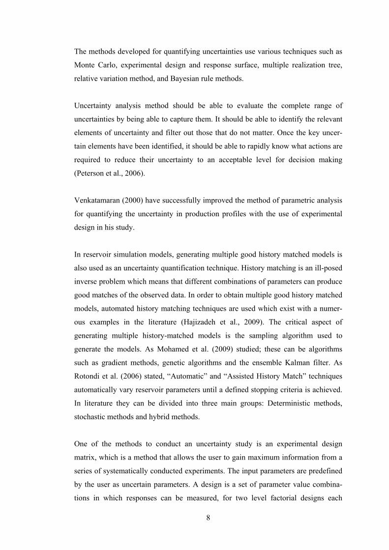
The cumulative oil production of the field by February 2011 is 1,443,425 bbl. The
field is currently producing from 4 wells (Bozova-1, 2, 3 and 8) at a total oil rate of
193 bbl/d, with a water cut of 75 %. The daily oil production graph of the field and
the bubble map illustrating the cumulative production of each well is given in Figure
3.2 and Figure 3.3.

11
Figure 3.1 Geographical location of Bozova field
Figure 3.2 The daily oil production graph of Bozova field
12
Figure 3.3 The bubble map the illustrating cumulative production of each well
3.2 Geological Description of the Field
3.2.1 Lithological Description of the Reservoir Level
In Bozova field, the oil producing zone is called Reservoir Level. The lithology of
this formation is bioclastic limestone and it is in the characteristics of calciturbudites.
This unit is formed by the migration from the shelf edge, is settled as small scale
channel fills and lenses around Bozova field. This Reservoir Level is so far observed
only in this field throughout the South-East Anatolian Region (Evin and Soyhan,
2004).

13
3.2.2 Structural Geology of the Field
The evolution of Bozova structure is thought to be passed through two tectonic
periods, one during Upper Cretaceous and the other one during Miocene
(Şengündüz, et al., 2000).
The first tectonic phase (Upper Cretaceous period) is the compression regime formed
by subduction of Arabian Plate underneath the Anatolian Plate. This compression
regime lead to drifting in northern areas, whereas leading to a deformation (folding
and faulting) in southern areas, the effect of which is decreasing towards south. The
compression trending northwest-southeast caused formation of folds trending
northeast-southwest and structures limited with reverse faults in the south.
The second major tectonic phase is the collision of Anatolian and Arabian Plates
which occurred 9 million years ago (Upper Miocene). The effect of this north-east
trending event in the northern areas is the overthrusting and drifting towards the
south. This effect decreases towards the southern areas. As a result folding, reverse
faults trending south and asymmetric anticlines extending east-west forms the
dominant topography.
In the formation of Bozova structure, 75 km length and high angled (approximately
85°) Bozova fault, trending northwest-southeast plays a key role. The Bozova fault
which has a right lateral throw was previously a normal and then a reverse fault in
the past.
Bozova field is an anticline structure limited with normal faults in the north and
south. There is a 10 km length fault trending north-south in the middle of the struc-
ture. This fault is considered to be permeable.

14
CHAPTER 4
STATEMENT OF THE PROBLEM
The primary objective of this study is to evaluate the impact of dynamic reservoir
uncertainties on the simulation results of Bozova oil field and ranking the simulation
models created for uncertainty evaluation. The study covers uncertainties associated
only to fluid properties, rock physics functions and WOC depth of the field.
Employing a full factorial experimental design, simulation models will be created for
all possible combinations of: 19 sets of Pc/krel curves taken from SCAL data; 2 sets
of PVT data obtained from PVT analyses of Bozova-1 and Bozova-3; and 3 sets of
WOC depths, which are considered to be informative on determination of the true
reservoir description.
Without pursuing the goal of a history matched case, 114 (2 x 3 x 19) simulation
models will be run. The results of the simulation runs will be plotted for screening
the impact of uncertainties. Following the screening, a history match analysis will be
processed on all of the simulation runs; history match values (corresponding to an
objective function showing the error between the simulated and observed data) will
be utilized to rank the simulation models. After ranking the models according to their
goodness of fit, quantification of uncertainties will be performed through two
different methods. Thus uncertainty evaluation will be assessed for the simulation
models of Bozova Field.

15
CHAPTER 5
METHOD OF SOLUTION
The commercial seismic-to-simulation software program Petrel is used for the
geological modeling; reservoir simulation; and history match analysis studies of
Bozova Field. Black oil simulator ECLIPSE 100 is used for the simulation runs.
5.1 Geological Modeling
5.1.1 Data Input, QA/QC
Basic well data including X, Y coordinates, kelly bushing elevation, measured depth,
formation depths, digital raw and processed logs of each well is imported into the
program. Wells sections illustrating the logs (porosity in the first, water saturation in
the second track), status, perforation and DST intervals of the wells are shown in
Figure 5.1. The Reservoir Level is the zone between the red dashed lines.
Figure 5.1 Well sections of Bozova field (Log process by Karakeçe, 2009)
16
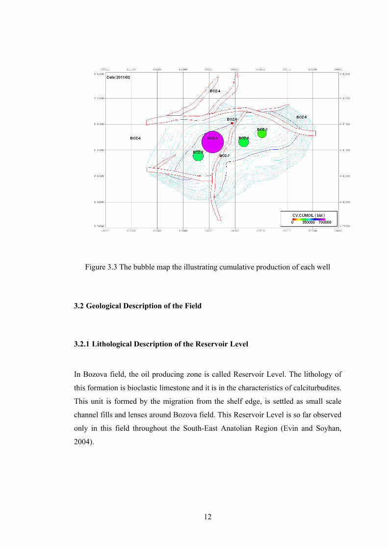
The structure contour map on top of Reservoir Level is imported into the program
and formations below are derived from this map (Figure 5.2).
Figure 5.2 Structure contour map of Bozova field on top of Reservoir Level (adapted from Sefunç & Ölmez, 2002)
5.1.2 3D Geological Grid and Petrophysical Parameter Modeling
The size of the grid cells are 50x50x1 m in the X, Y and Z directions respectively.
The number of active grid cells is 101,904. Z values ranging from 3 to 15 m are
assigned to the formations below the Reservoir Level.
By using Sequential Gaussian Simulation geostatistical method and variogram
models porosity values determined from logs are distributed throughout the field. By
using the porosity-permeability plot obtained from core data porosity cut-off is
identified as 13 % (Figure 5.3). Water saturation values are distributed by using a
height dependent function. Porosity and water saturation properties are shown in
Figure 5.4 and Figure 5.5.

17
Figure 5.3 The porosity-permeability plot obtained from core data
Figure 5.4 Porosity distribution model of the 3D grid

18
Figure 5.5 Sw distribution model of the 3D grid
5.1.3 STOOIP Calculation from 3D Geological Model
The deterministic reserve calculation is done with 3 WOC depths of 1455, 1468 and
1480 m ssTVD. The stock tank oil originally in place (STOOIP) amounts are volu-
metrically calculated as 18.5, 28.1, 34.2 million bbls respectively. These values are
consistent with the simulation results that are given in the further chapters.
5.2 Basic Reservoir Engineering
This section covers the basic reservoir engineering tasks that are performed in order
to understand the dynamics of the reservoir. Before jumping into the simulation, a
comprehensive study is performed for collection of basic reservoir engineering data,
which is of primary importance in generating the dynamic model accurately. Also
determination of uncertainties in WOC, Pc/krel curves and PVT data are performed.
19
5.2.1 Well Test Interpretations
A total number of 10 open hole DSTs were performed in the Reservoir Level of
wells Bozova-1, 2, 3, 4, 5, 8 and 9 between years 1995 and 1998. All of the tests
consisted of two flow and two shut-in periods.
Since the bottom hole pressure gauges which are run in hole are mechanical, there
may be a significant uncertainty in the BHP values. Calibration of the gauges and the
accuracy of calculation of pressure values from the charts are of major importance.
Also the flow data were not measured during the tests. They were determined by
complex calculations that use the pressure gradient of the recovered fluid, hydrostat-
ic pressure differential during flow period, the related fluid volume in the test string
and the duration of the flow. All of these factors bring a certain amount of uncertain-
ty to the calculations of flow rates. The rates are double-checked to see if the
derivative of the pressure differentials coming from the 1st and the 2nd shut-in build-
up periods were consistent.
Test interpretations are performed by Ecrin Pressure Transient Analysis Module
(KAPPA Software). The final shut-in period of the well tests are analyzed by using
Log-log and Horner analysis. The reservoir parameters, such as original reservoir
pressure (Pi), permeability (k) and skin factor (S) are obtained from these interpreta-
tions. Interpreted well test details, parameters used for interpretation and the results
are given in Table 5.1. Log-log, semi-log and history plots of all the interpreted well
tests are given in Appendix A.

20
Table 5.1 Bozova DST parameters and the interpretation results
Wel
lB
oz-1
Boz
-1B
oz-2
Boz
-2B
oz-3
Boz
-4B
oz-4
Boz
-5B
oz-8
Boz
-9D
ST
No
12
12
11
21
11
Inte
rval
, m19
12.5
- 19
2619
30.6
- 19
46.5
1912
.5 -
1926
1930
.4 -
1952
1892
.8 -
1908
.819
50 -
1967
1964
- 19
8719
55 -
1969
1896
.9 -
1916
1911
-193
2D
ate
07.1
1.19
9509
.11.
1995
01.0
1.19
9703
.01.
1997
30.1
1.19
9601
.09.
1997
03.0
9.19
9708
.11.
1997
25.0
9.19
9816
.12.
1998
Pa
ram
ete
rs U
sed
Wel
l Rad
ius,
in4.
254.
254.
254.
254.
254.
254.
256.
125
4.25
4.25
Gau
ge D
epth
, m s
sTV
D-1
433
-145
4-1
417
-143
5-1
431
-150
6-1
526
-149
0-1
448
-143
7N
et p
ay z
one,
m6.
8615
.85
10.5
117
.07
8.53
6.86
22.5
611
.74
16.6
112
.80
Por
osity
, %20
.94
18.6
420
.29
17.0
919
.28
4.34
5.09
19.4
120
.55
16.1
2S
w, %
17.5
519
.25
26.5
231
.19
21.5
817
.26
15.4
852
.28
23.0
730
.14
Tem
pera
ture
, o F20
017
017
017
416
817
817
918
017
217
61s
t Flo
w R
ate,
bbl
/day
235
240
256
173
190
7017
054
027
014
02n
d Fl
ow R
ate,
bbl
/day
170
110
202
114
130
4010
032
016
070
Flu
id P
rop
ert
ies*
AP
I22
.922
.922
.922
.922
.922
.922
.922
.922
.922
.9O
il Fo
rm. V
ol. F
ac.,
rm3 /s
m1.
053
1.04
21.
042
1.04
31.
041
1.04
51.
045
1.04
61.
043
1.04
4V
isco
sity
, cp
5.04
77.
793
7.79
37.
298
8.06
26.
852
6.74
86.
646
7.53
97.
069
Tota
l Com
pres
sibi
lity,
psi
-18.
24E
-06
6.49
E-0
66.
81E
-06
6.88
E-0
66.
44E
-06
6.96
E-0
67.
00E
-06
6.45
E-0
67.
18E
-06
7.17
E-0
6
Re
sult
sk,
mD
12.6
4.9
33.0
4.7
17.1
3.3
2.6
18.6
9.4
3.4
S0.
171
0.16
04.
003
0.27
11.
351
-0.0
48-0
.200
0.02
60.
352
-0.1
92P
i, ps
ia25
7926
1223
2523
8725
7826
2326
4827
7621
5622
45P
I bbl
/d/p
si
*At P
i and
give
n te
mpe
ratu
re.
Res
. Lev
elR
es. L
evel
Res
. Lev
elR
es. L
evel
Res
. Lev
elR
es. L
evel
Res
. Lev
.Fo
rmat
ion
Res
. Lev
elR
es. L
evel
Res
. Lev
el

21
5.2.2 Bottom Hole Pressure (BHP) Measurements
The BHP of wells Bozova-1, 3 and 8 are measured right before their production start
up between years 1995 and 1998. The measurements were made at different levels
by running the gauge into the well and pulling it to the next upper level. The gauge
was assumed to be kept at each level for an enough period of time that the pressure
values were considered to be stabilized. Another set of BHP measurements were
made with Spartek digital pressure gauge in wells Bozova-2, 8 and 9 in February
2011. The details of each BHP measurement are given in Appendix B.
5.2.3 Determination of Original Reservoir Pressure (Pi)
The pressure values obtained from DST interpretation results and BHP measure-
ments are shown in Table 5.2. All of the pressure values (corrected at a reference
depth of 1455 m ssTVD) are plotted on a date vs. pressure graph in Figure 5.6.
Table 5.2 Pressure values obtained from DSTs and BHP measurements
Gauge Depth BHP Pres. Grad. BHP @-1455 m.m psi psi/m psi
BOZ-1 DST#1_Nov '95 -1433 2579 1.406 2610BOZ-1 DST#2_Nov '95 -1454 2612 1.406 2614BOZ-2 DST#1_Jan '97 -1417 2325 1.301 2374BOZ-2 DST#2_Jan '97 -1435 2387 1.301 2413BOZ-3 DST#1_Nov '96 -1431 2578 1.206 2607
DST BOZ-4 DST#1_Sep '97 -1506 2623 1.301 2557BOZ-4 DST#2_Sep '97 -1526 2648 1.301 2556BOZ-5 DST#1_Nov '97 -1490 2776 1.301 2731BOZ-8 DST#1_Sep '98 -1448 2156 1.275 2165BOZ-9 DST#1_Dec '98 -1437 2245 1.301 2268
BOZ-1 AMRD-1_Dec '95 -1432 2482 1.406 2514AMERADA BOZ-1 AMRD-2_Dec '95 -1432 2454 1.396 2486
(MECHANICAL BOZ-3 AMRD-1_Feb '97 -1418 2022 1.215 2067GAUGE) BOZ-3 AMRD-2_Feb '97 -1418 1970 1.207 2015
BOZ-8 AMRD-1_Oct '98 -1439 1729 1.288 1750BOZ-8 AMRD-2_Oct '98 -1439 1756 1.275 1777
SPARTEK BOZ-2 SPRTK-1_Feb '11 -852 1496 1.408 2345(DIGITAL BOZ-8 SPRTK-1_Feb '11 -1239 1314 1.409 1618GAUGE) BOZ-9 SPRTK-1_Feb '11 -1400 2017 1.368 2092
Well & BHP Name

22
0
500
1000
1500
2000
2500
3000
1993 1995 1998 2001 2004 2006 2009 2012
Pre
ssur
e, p
si
BOZ-1 DST#1_Nov '95
BOZ-1 DST#2_Nov '95
BOZ-1 AMRD-1_Dec '95
BOZ-1 AMRD-2_Dec '95
BOZ-3 DST#1_Nov '96
BOZ-2 DST#1_Jan '97
BOZ-2 DST#2_Jan '97
BOZ-3 AMRD-1_Feb '97
BOZ-3 AMRD-2_Feb '97
BOZ-4 DST#1_Sep '97
BOZ-4 DST#2_Sep '97
BOZ-5 DST#1_Nov '97
BOZ-8 DST#1_Sep '98
BOZ-8 AMRD-1_Oct '98
BOZ-8 AMRD-2_Oct '98
BOZ-9 DST#1_Dec '98
BOZ-2 SPRTK-1_Feb '11
BOZ-8 SPRTK-1_Feb '11
BOZ-9 SPRTK-1_Feb '11
ignoredAmerada
BHP values
Figure 5.6 Date vs. pressure plot of pressure values corrected @1455 m ssTVD
The Amerada BHP values of Bozova-3 and 8 are much lower than their DST pres-
sure values. This inconsistency may be stemming from the unstabilized pressure
readings of the Amerada BHP measurements and because of their questionable
reliability they are not taken into account in further steps of this study.
In order to determine the original reservoir pressure (Pi), the pressure values that are
measured before the production beginning of wells are plotted on a pressure vs.
depth graph in Figure 5.7. As clearly seen in this figure, pressure values show a wide
distribution which makes it difficult to decide on Pi and they are examined to identi-
fy the ones that should be taken into account and the ones that should be ignored.
23
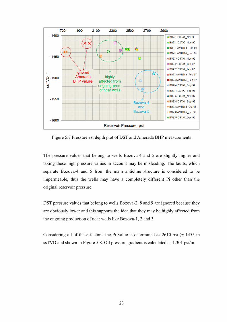
Figure 5.7 Pressure vs. depth plot of DST and Amerada BHP measurements
The pressure values that belong to wells Bozova-4 and 5 are slightly higher and
taking these high pressure values in account may be misleading. The faults, which
separate Bozova-4 and 5 from the main anticline structure is considered to be
impermeable, thus the wells may have a completely different Pi other than the
original reservoir pressure.
DST pressure values that belong to wells Bozova-2, 8 and 9 are ignored because they
are obviously lower and this supports the idea that they may be highly affected from
the ongoing production of near wells like Bozova-1, 2 and 3.
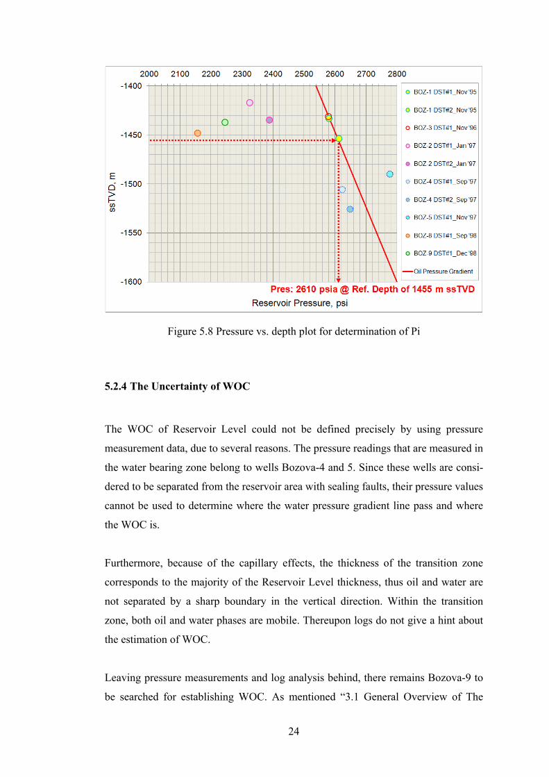
Considering all of these factors, the Pi value is determined as 2610 psi @ 1455 m
ssTVD and shown in Figure 5.8. Oil pressure gradient is calculated as 1.301 psi/m.
24
Figure 5.8 Pressure vs. depth plot for determination of Pi
5.2.4 The Uncertainty of WOC
The WOC of Reservoir Level could not be defined precisely by using pressure
measurement data, due to several reasons. The pressure readings that are measured in
the water bearing zone belong to wells Bozova-4 and 5. Since these wells are consi-
dered to be separated from the reservoir area with sealing faults, their pressure values
cannot be used to determine where the water pressure gradient line pass and where
the WOC is.
Furthermore, because of the capillary effects, the thickness of the transition zone
corresponds to the majority of the Reservoir Level thickness, thus oil and water are
not separated by a sharp boundary in the vertical direction. Within the transition
zone, both oil and water phases are mobile. Thereupon logs do not give a hint about
the estimation of WOC.
Leaving pressure measurements and log analysis behind, there remains Bozova-9 to
be searched for establishing WOC. As mentioned “3.1 General Overview of The

25
Field” Bozova-9 was abandoned shortly after (11 months later) its water production
percentage reaching 100 %. The tested perforation interval is 1918 – 1930 m,
corresponding to 1453 – 1465 m ssTVD. The WOC penetrated in Bozova-9 might be
at the depth of (top of perforation) 1453 m ssTVD, or (bottom of perforation) 1465
m ssTVD. Regarding the possibility of “WOC being at the bottom depth for Reser-
voir Level” and “the perforation gets connected with the WOC after a short period of
production” 1477 m ssTVD is also a candidate for WOC.
Taking all of these factors into consideration, the uncertainty of WOC depth is
studied through 3 different values which are considered to be informative on deter-
mination of the true reservoir description. Rounding and leaving equal intervals
between the numbers, WOC depths to be studied in uncertainty analysis are taken as
1455, 1468 and 1480 m ssTVD (Figure 5.9).

26
Figure 5.9 WOC depths studied in uncertainty analysis
(1455, 1468 and 1480 m ssTVD)
27
5.2.5 The Uncertainty in Pc/Krel Curves
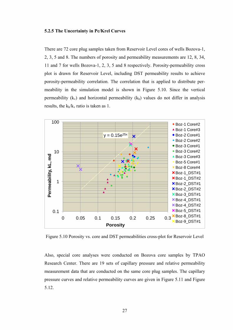
There are 72 core plug samples taken from Reservoir Level cores of wells Bozova-1,
2, 3, 5 and 8. The numbers of porosity and permeability measurements are 12, 8, 34,
11 and 7 for wells Bozova-1, 2, 3, 5 and 8 respectively. Porosity-permeability cross
plot is drawn for Reservoir Level, including DST permeability results to achieve
porosity-permeability correlation. The correlation that is applied to distribute per-
meability in the simulation model is shown in Figure 5.10. Since the vertical
permeability (kv) and horizontal permeability (kh) values do not differ in analysis
results, the kh/kv ratio is taken as 1.
y = 0.15e25x
0.1
1
10
100
0 0.05 0.1 0.15 0.2 0.25 0.3
Per
mea
bili
ty, k
L, m
d
Porosity
Boz-1 Core#2Boz-1 Core#3Boz-2 Core#1Boz-2 Core#2Boz-3 Core#1Boz-3 Core#2Boz-3 Core#3Boz-5 Core#1Boz-8 Core#4Boz-1_DST#1Boz-1_DST#2Boz-2_DST#1Boz-2_DST#2Boz-3_DST#1Boz-4_DST#1Boz-4_DST#2Boz-5_DST#1Boz-8_DST#1Boz-9_DST#1
Figure 5.10 Porosity vs. core and DST permeabilities cross-plot for Reservoir Level
Also, special core analyses were conducted on Bozova core samples by TPAO
Research Center. There are 19 sets of capillary pressure and relative permeability
measurement data that are conducted on the same core plug samples. The capillary
pressure curves and relative permeability curves are given in Figure 5.11 and Figure
5.12.

28
Even though the curves seem to be close to each other, their Swir values show a
range between 0.05 and 0.18 and Swir is a key parameter while determining the oil
in place. Similarly relative permeability curves assign the fundamental rules of flow
functions. In order to investigate the impacts of Pc/krel curves on the simulation
results they are studied through 19 sets of data.
Figure 5.11 Capillary pressure curves for Reservoir Level
Figure 5.12 Relative permeability curves for Reservoir Level
29
5.2.6 The Uncertainty in Fluid Properties
The uncertainties of the reservoir properties, such as the geologic and petrophysical
data, are often given more attention than the uncertainties of the fluid properties. The
uncertainty of fluid property measurements affect the quality of fluid property data
which in turn affecting the accuracy of simulation models. In addition to the incon-
sistency from the measurements, fluid sampling is another main source contributing
to the accuracy of fluid property data. Therefore, it is essential to study the effect of
the variation in fluid properties, such as oil viscosity, compressibility and bubble
point pressure values to generate accurate reservoir simulation models.
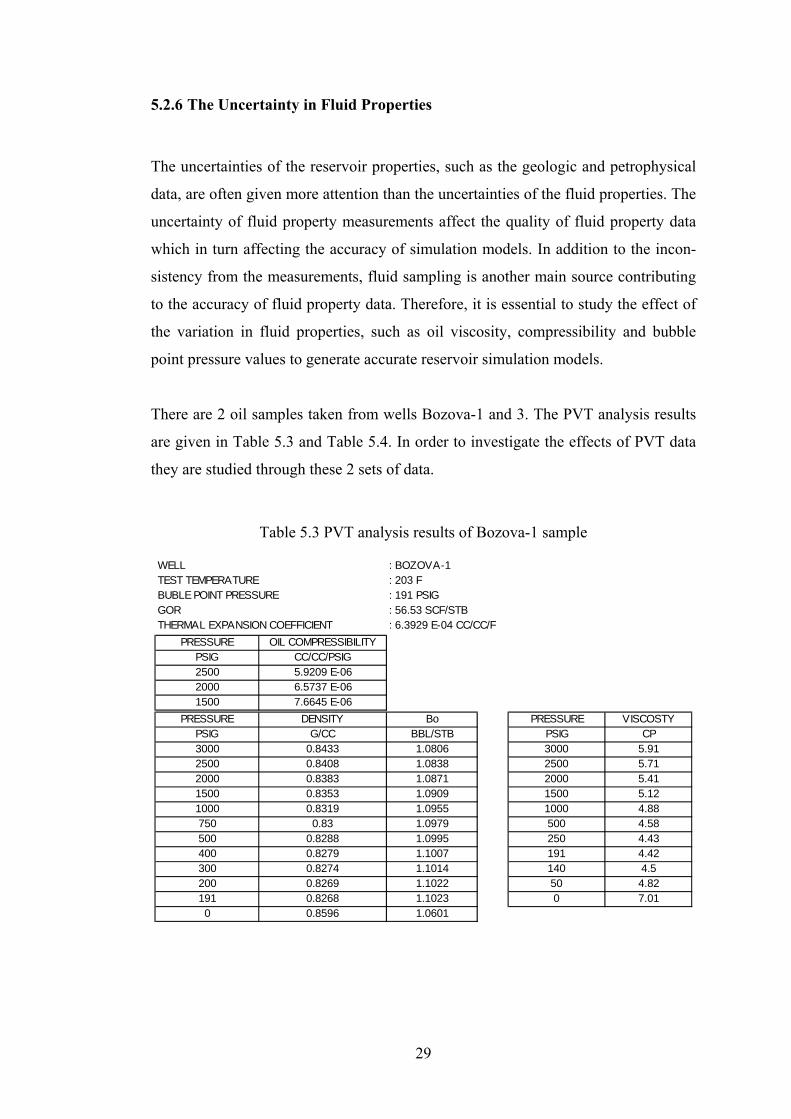
There are 2 oil samples taken from wells Bozova-1 and 3. The PVT analysis results
are given in Table 5.3 and Table 5.4. In order to investigate the effects of PVT data
they are studied through these 2 sets of data.
Table 5.3 PVT analysis results of Bozova-1 sample
WELL : BOZOVA-1TEST TEMPERATURE : 203 FBUBLE POINT PRESSURE : 191 PSIGGOR : 56.53 SCF/STBTHERMAL EXPANSION COEFFICIENT : 6.3929 E-04 CC/CC/F
PRESSURE OIL COMPRESSIBILITYPSIG CC/CC/PSIG2500 5.9209 E-062000 6.5737 E-061500 7.6645 E-06
PRESSURE DENSITY Bo PRESSURE VISCOSTYPSIG G/CC BBL/STB PSIG CP3000 0.8433 1.0806 3000 5.912500 0.8408 1.0838 2500 5.712000 0.8383 1.0871 2000 5.411500 0.8353 1.0909 1500 5.121000 0.8319 1.0955 1000 4.88750 0.83 1.0979 500 4.58500 0.8288 1.0995 250 4.43400 0.8279 1.1007 191 4.42300 0.8274 1.1014 140 4.5200 0.8269 1.1022 50 4.82191 0.8268 1.1023 0 7.010 0.8596 1.0601

30
Table 5.4 PVT analysis results of Bozova-3 sample
WELL : BOZOVA-3TEST TEMPERATURE : 170 FBUBLE POINT PRESSURE : 231 PSIGGOR : 59.4 SCF/STBTHERMAL EXPANSION COEFFICIENT : 6.2620 E-04 CC/CC/F
PRESSURE OIL COMPRESSIBILITYPSIG CC/CC/PSIG2000 5.9270 E-061000 6.2494 E-06400 6.4640 E-06
PRESSURE DENSITY Bo PRESSURE VISCOSTYPSIG G/CC BBL/STB PSIG CP3000 0.8822 1.0476 3000 10.22000 0.8755 1.0532 2000 9.21000 0.8719 1.06 1000 8.2500 0.869 1.0636 500 7.9400 0.8684 1.0643 300 7.7300 0.8679 1.0648 231 7.6231 0.8675 1.0653 0 10.10 0.8845 1.0449
5.3 Reservoir Simulation
The parameters, the effects of which are going to be studied in the simulation
modeling, are determined in “5.2 Basic Reservoir Engineering”. These are:
1. WOC depth (3 possible values),
2. Pc and krel curves (19 sets of SCAL data),
3. Oil PVT behavior (2 sets of PVT analysis data).
Following a full factorial experimental design, the combination of these parameters
will give a total of 114 (3 x 2 x 19) cases to be simulated. The experimental design
table showing the combination of uncertain variables and corresponding case names
is given in Appendix C.
5.3.1 Making Fluid Model
6 fluid models for 2 PVT and 3 WOC sets are prepared. The factorial design for fluid
modeling is given in Table 5.5.

31
Table 5.5 The factorial design for fluid modeling
Fluid Model PVT WOCFM1 Boz-1 -1455FM2 Boz-1 -1468FM3 Boz-1 -1480FM4 Boz-3 -1455FM5 Boz-3 -1468FM6 Boz-3 -1480
Initial conditions are entered into the model as mentioned in “5.2.3 Determination of
Original Reservoir Pressure”, given in Table 5.6.
Table 5.6 Initial conditions
Ref. Depth, m Pressure, psia Temperature, ºF-1455 2610 177
5.3.2 Making Rock Physics Functions
Relative permeability and capillary pressure data for each core plug sample are
entered into the rock physics functions as spreadsheets (Figure 5.13 and Figure
5.14).

32
Figure 5.13 Smoothed relative permeability curves taken from SCAL data
Figure 5.14 Smoothed capillary pressure curves taken from SCAL data
33
5.3.3 Making Aquifer Model
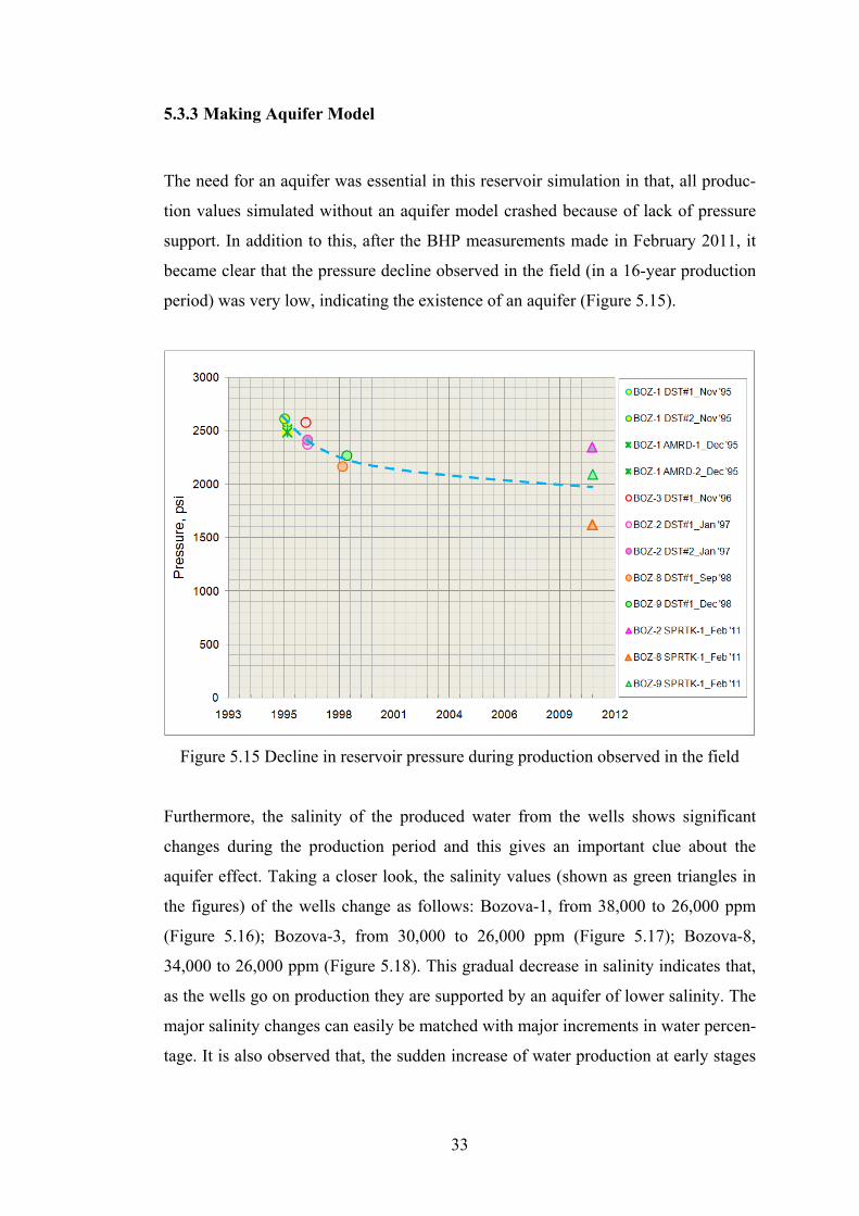
The need for an aquifer was essential in this reservoir simulation in that, all produc-
tion values simulated without an aquifer model crashed because of lack of pressure
support. In addition to this, after the BHP measurements made in February 2011, it
became clear that the pressure decline observed in the field (in a 16-year production
period) was very low, indicating the existence of an aquifer (Figure 5.15).
Figure 5.15 Decline in reservoir pressure during production observed in the field
Furthermore, the salinity of the produced water from the wells shows significant
changes during the production period and this gives an important clue about the
aquifer effect. Taking a closer look, the salinity values (shown as green triangles in
the figures) of the wells change as follows: Bozova-1, from 38,000 to 26,000 ppm
(Figure 5.16); Bozova-3, from 30,000 to 26,000 ppm (Figure 5.17); Bozova-8,
34,000 to 26,000 ppm (Figure 5.18). This gradual decrease in salinity indicates that,
as the wells go on production they are supported by an aquifer of lower salinity. The
major salinity changes can easily be matched with major increments in water percen-
tage. It is also observed that, the sudden increase of water production at early stages

34
of production is taken under control successfully by narrowing the perforation
intervals in wells Bozova-1 and 3.
Figure 5.16 Test and production graph of Bozova-1
Figure 5.17 Test and production graph of Bozova-3

35
Figure 5.18 Test and production graph of Bozova-8
The only well that produces low salinity water from the beginning of its production
is Bozova-2, salinity of which changes only from 5,000 to 3,000 ppm (Figure 5.19).
Figure 5.19 Test and production graph of Bozova-2

36
As a result of all these considerations the aquifer is conceived to be an edge water
drive aquifer supporting the field from an area close to Bozova-2, in a direction from
south to the rest of the field. After some small scale sensitivity analysis concerning
the area and the strength of the aquifer, it is connected to the bottom of Reservoir
Level, with a bottom to top and edge drive definition. (Figure 5.20).
Figure 5.20 Aquifer connected to the bottom of Reservoir Level
5.3.4 Running the Simulation Models
The development strategies are generated for history matching purposes. Oil produc-
tion rate is chosen as the production control mode. The limiting bottom hole pressure
is taken as the bubble point pressure.
The average execution time for a single simulation was about 3 minutes on a com-
puter with an Intel® Core™2 Duo CPU 3.16 GHz processor and 3.48 GB RAM. The
total time required to run 114 simulation models is about 6 hours. Since this time
period is considered to be moderate, the idea of running all possible cases is applied.

37
5.4 History Match Analysis
History match analysis is used to quantify how well the simulation models reproduce
the observed well data. In order to quantify match values root mean square (RMS)
technique is used. RMS signifies the calculated error for every point. The bigger the
RMS value the worse the match of the simulation model with the observed well data.
N
i
OiSi
NM
1
21
(5.1)
Where:
M is the match value.
S is the simulated value.
O is the observed value.
N is the number of points ( i ) that is used to compute M .
is a normalization parameter that is used to make sure all the match values are in
the same order of magnitude.
The normalization parameter is used to assign one vector, or a selection of the
vectors, different weighting factors when combining matches. It makes the match
unitless and makes the result in a certain normalized range. The “Average (%)”
option divides the error (difference between simulated and observed) with the
percentage of the average observed value, whereas “Absolute” option uses the
specified value. By using an absolute value of 1, the match value will be the un-
weighted average error in the original unit.
Sampling frequency is chosen as simulation or observed frequency. Simulation
frequency averages the observed data and compares with the simulated data at every
time step. Observed frequency compares the simulated values at all observed data
points.
Sometimes improving one match can worsen the other. In order to clarify such
contradicting match evaluations a combined vector match, which takes all of the

38
vector matches into account, is essential. The calculation for a combined vector is
performed in the following way:
vectors wells
vectors wellsvectorswells
ncombinatio
MM
)1(
)( 2),(
)( (5.2)
The individual settings specified for the vectors used in this study is shown in Table
5.7.
Table 5.7 Normalization parameters for combined vector match
Vector Match Normalization FrequencyWater Cut Absolute, 1 SimulationWater Production Rate Average(%), 10 SimulationOil Production Rate Average(%), 10 SimulationWater Production Cumulative Average(%), 10 SimulationOil Production Cumulative Average(%), 10 SimulationBottom Hole Pressure Average(%), 10 Observed
Since it is more reliable to use rates rather than ratios such as water cut, the weight
factor for water cut vector is given an absolute value of 1. The remaining vectors are
set to an average normalization parameter of 10 %. The only vector, the sampling
frequency of which is set to observed, is the BHP.
5.5 Two Level (2k) Factorial Design Technique as an Uncertainty Quantification Method
For the purpose of obtaining information in an efficient and less time consuming
way, statistically designed experiments are used. If the purpose of the experimenta-
tion is to determine the important variables, the factorial designs are extremely
useful. Factorial designs also provide the combined effect of two or more variables
(Saxena and Pavelic, 1971).
In factorial designs, conditions are chosen by selecting a fixed number of levels for
each variable and then experiments are run at all possible combinations. A special

39
case of factorial designs is “Two Level Factorial Designs”. These designs are usually
written as 2k designs, where 2 denotes the number of levels of each variable and k is
the number of the variables under investigation. The number of experiments that are
to be performed for the factorial designs is given in as:
Number of experiments = 2k (5.3)
In order to explain through an example, a 2k design is constructed and analyzed for
three variables: x1, x2 and x3. For all three variables, the effects of which are to be
searched, two levels are identified: one as “high” and one as “low”. A coding system
is used so that “+1” denotes the high level, and “-1” denotes the low level, just to
simplify the design. The 2k factorial design for the three variables require eight (23)
tests. The design matrix is given in Table 5.8, which gives the combination of the
experiments that are to be performed. After designing the experiment, the tests are
performed and the responses (y) are obtained.
Table 5.8 Coded design matrix with results
Test Run No x1 x2 x3 y
1 -1 -1 -1 y1
2 +1 -1 -1 y2
3 -1 +1 -1 y3
4 +1 +1 -1 y4
5 -1 -1 +1 y5
6 +1 -1 +1 y6
7 -1 +1 +1 y7
8 +1 +1 +1 y8
If the three variables are considered as three mutually perpendicular coordinate axes
x1, x2, x3, the 23 factorial design can be geometrically represented as a cube shown in
Figure 5.21.

40
Figure 5.21 Geometrical representation of the 23 design (adapted from Saxena and Pavelic, 1971)
Once the tests are performed and the results are obtained, the influence of each
variable on the response can be obtained by calculating the average effects. For
example; in Figure 5.21, for test number 1 and 2, the conditions of x2 and x3 are the
same but x1 conditions are different, i.e., high level of x1 is used for test 2 while a
low level is used for test 1. Similarly, for the pairs of test 3 and 4; 5 and 6; 7 and 8,
each pair involves similar test conditions with respect to x2 and x3 but different test
conditions with respect to x1. Thus, the difference in the results within each of these
pairs reflects the effect of x1 alone. To calculate the overall average effect of x1, the
four differences are averaged as shown in Equation 5.4.
4
)()()()( 785634121
yyyyyyyyE
(5.4)
Geometrically, the average effect of x1 (E1) is simply the difference between the
average results on a plane at high level of x1 and the average result on a plane at low
level of x1. The high and low level planes for all variables x1, x2 and x3 are shown in
Figure 5.22.

41
Figure 5.22 The high and low level planes for variables x1, x2 and x3 (adapted from Saxena and Pavelic, 1971)
In general, the average effect is computed as in Equation 5.5.
level) lowat sy' of (Average - level)high at sy' of (AverageEffect Average (5.5)
In order to calculate the interaction between x1 and x2 (E12), compressing the cube in
the direction of x3, the cube is transformed into a square as shown in Figure 5.23.
The diagonal representing the high plane includes tests 1, 5, 4 and 8; whereas the
low plane consists of tests 2, 6, 3 and 7.
Figure 5.23 The high and low level planes for calculating the interaction between x1 and x2 (E12) (adapted from Saxena and Pavelic, 1971)

42
The interaction between x1 and x2 can be calculated by Equation 5.6.
plane) lowat sy' of (Average - plane)high at sy' of (Average E12 (5.6)
There is also a simplified method in order to calculate two and three-factor interac-
tions. The first step is to obtain a calculation matrix from the design matrix. This is
done by multiplying all the columns of the design matrix in all possible ways. The
multiplication of the columns is done by multiplying the corresponding elements of
the columns. For example column x1x3 is obtained as:
3131
1
1
1
1
1
1
1
1
1
1
1
1
1
1
1
1
1
1
1
1
1
1
1
1
xColumnxColumnxColumnx
x
(5.7)
The complete calculation matrix along with the design matrix and the results y, are
shown in Table 5.9.
Table 5.9 Design and calculation matrix; and the results (Saxena and Pavelic, 1971)
Test Run No x1 x2 x3 x1x2 x1x3 x2x3 x1x2x3 y
1 -1 -1 -1 +1 +1 +1 -1 y1
2 +1 -1 -1 -1 -1 +1 +1 y2
3 -1 +1 -1 -1 +1 -1 +1 y3
4 +1 +1 -1 +1 -1 -1 -1 y4
5 -1 -1 +1 +1 -1 -1 +1 y5
6 +1 -1 +1 -1 +1 -1 -1 y6
7 -1 +1 +1 -1 -1 +1 -1 y7
8 +1 +1 +1 +1 +1 +1 +1 y8
DESIGN MATRIX CODED
CALCULATION MATRIX

43
The average effects and the interactions are then computed by multiplying the
relevant column with the column y and dividing by the number of plus signs in the
column. For example the average effect of E2 is calculated as follows:
yColumnxColumn
y
y
y
y
y
y
y
y
xxxcolumninsignsplusofNumber
E
.8
7
6
5
4
3
2
1
2.
22
1
1
1
1
1
1
1
1
......
1
(5.8)
The three-factor interaction E123 is:
yColumnxxxColumn
y
y
y
y
y
y
y
y
xxxxxcolumninsignsplusofNumber
E
.8
7
6
5
4
3
2
1
3.2.1.
321123
1
1
1
1
1
1
1
1
......
1
(5.9)
The analysis of the results can be carried out by ranking the effects and interactions
according to the absolute magnitudes.

44
CHAPTER 6
RESULTS AND DISCUSSIONS
6.1 Screening the Simulation Results
A total number of 114 simulation runs are conducted for the uncertainty evaluation,
without pursuing the goal of a history matched best case. In order to visualize the
results of the simulations according to their goodness of fit, they are viewed in many
different aspects. In order to clearly visualize the over-lapping results, the plots are
separated in two groups according to the used fluid model; first group as FM1, FM2
and FM3; second group as FM4, FM5 and FM6. First group models (FM-1, 2, 3) use
the PVT data of Bozova-1 (which will be named as PVT-1) and the second group
models (FM-4, 5, 6) use the PVT data of Bozova-3 (which will be named as PVT-3).
The details of fluid models are given in “5.3.1 Making Fluid Model”.
6.1.1 Production Rate Results
The oil and water production rate results for the simulations are shown in Figure 6.1
(PVT-1), Figure 6.2 (PVT-3); and in Figure 6.3 (PVT-1) and Figure 6.4 (PVT-3)
respectively. As clearly seen in figures, the results of the simulations that have the
same fluid model are grouped as being close to each other. Fluid model is con-
structed upon combination of 2 items; WOC and PVT properties. When the results of
first group (FM1, 2, 3 that belong to PVT-1) is compared to the results of the second
group (FM-4, 5, 6 that belong to PVT-3) it is easy to say that uncertainty of PVT
data make a minor impact on the results; but it is difficult to decide whether WOC
depth is or Pc/krel curves are more determinant on the production rate results. This is
an issue to be clarified after history match analysis results.

45
Figure 6.1 Oil production rates of simulation models (PVT-1: FM1,2,3)

46
Figure 6.2 Oil production rates of simulation models (PVT-3: FM4,5,6)

47
Figure 6.3 Water production rates of simulation models (PVT-1: FM1,2,3)
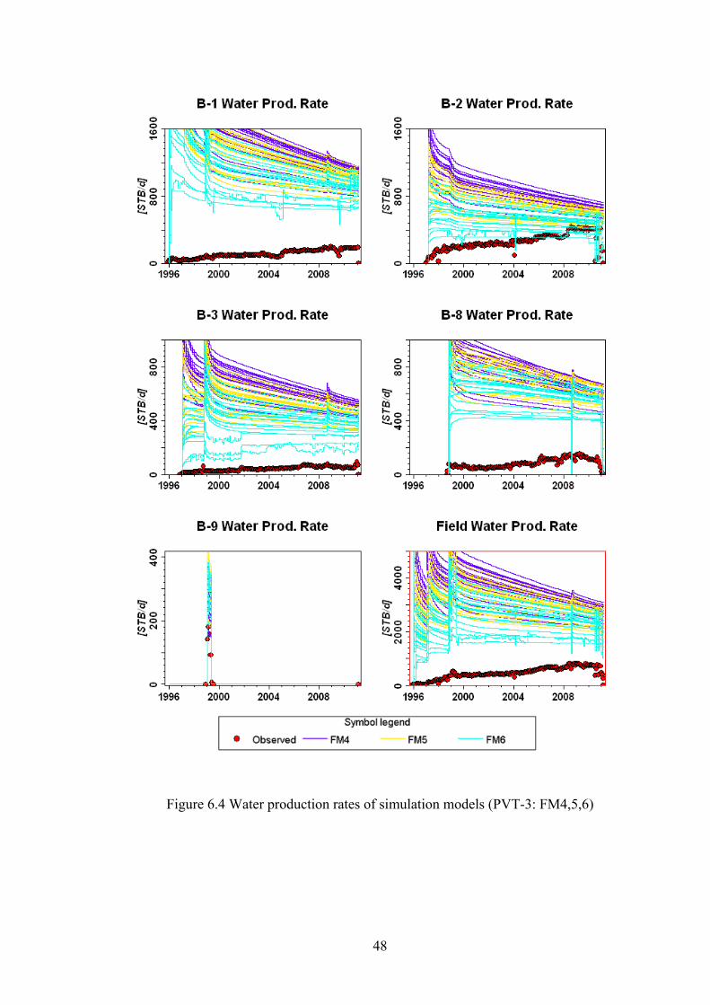
48
Figure 6.4 Water production rates of simulation models (PVT-3: FM4,5,6)

49
Indicating a WOC of 1480 m ssTVD, simulation cases of FM3, FM6 are the best
matched models. Also FM2, having a WOC of 1468 m ssTVD, shows matched
results for some of the wells. The worst matched simulation models FM1 and FM4
are not capable of producing the target oil production rates even if they produce too
much water. The goodness of the water production rate results is parallel to the
goodness of the oil production rate results in that, as the water production rate results
get closer to the observed data, oil production rate results also get closer to the
observed data.
The reason why PVT-1 model results show better match depends on the fact that
PVT-1 has lower viscosity values than PVT-3. This situation directly affects the
mobility ratio of oil. Also higher initial GOR values result in higher oil production
because gas enhances the recovery performance. But this is not the main point for
the different behaviours of the 2 PVT groups because their initial GOR values do not
show a large variation. Another determinant is the oil compressibility value, which is
a source of energy for fluid flow in the reservoir. The oil compressibility of PVT-1 is
higher than the oil compressibility of PVT-3, which again favors the results of PVT-
1 simulation models.
6.1.2 Cumulative Production Results
The cumulative oil and water production rate results for the simulations are shown in
Figure 6.5, Figure 6.6 and in Figure 6.7 and Figure 6.8 respectively. The same
reasons aforementioned in “6.1.1 Production Rate Results” again explains the
matched models. The most effective variables on cumulative production results are
depth of WOC level and Pc/krel curves.
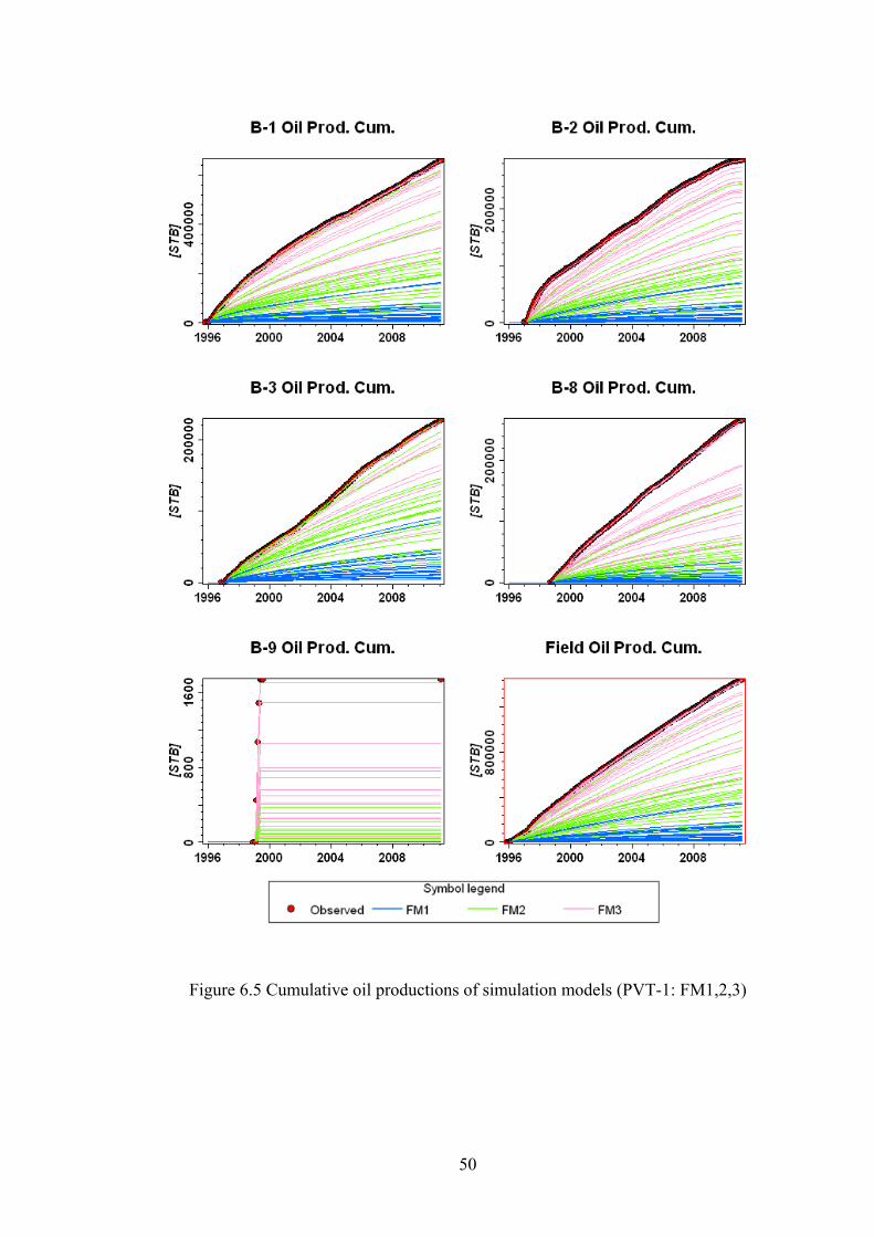
50
Figure 6.5 Cumulative oil productions of simulation models (PVT-1: FM1,2,3)
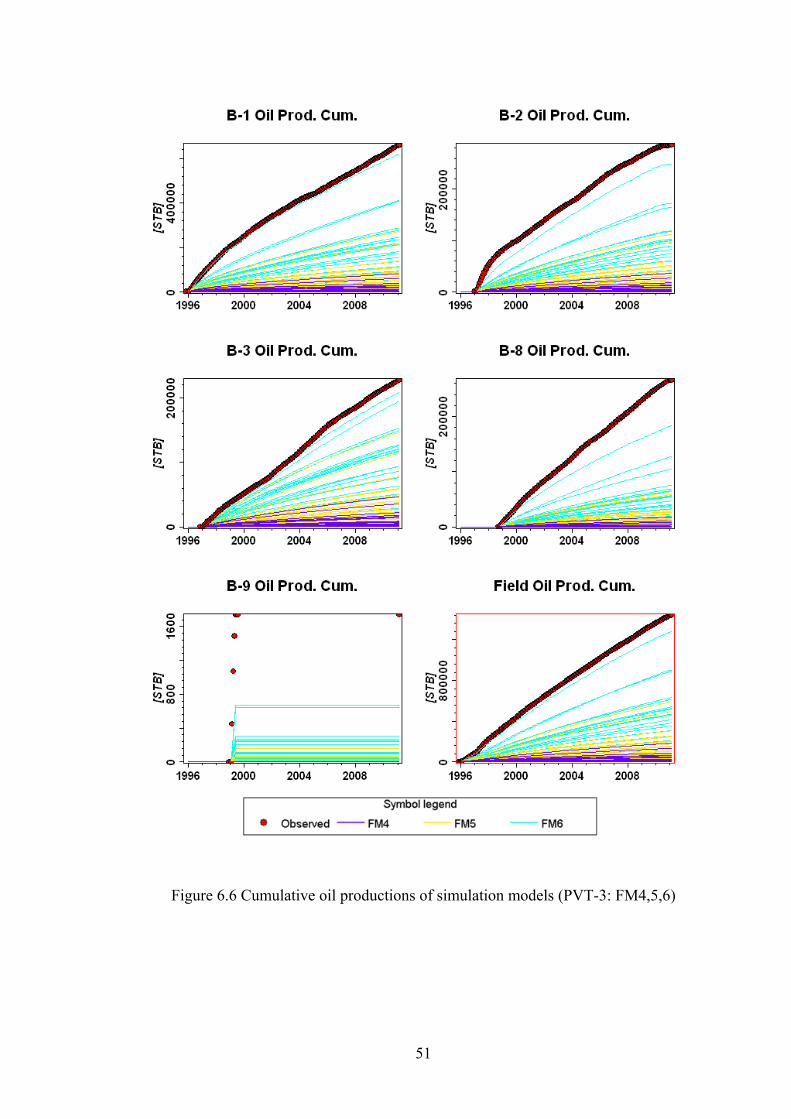
51
Figure 6.6 Cumulative oil productions of simulation models (PVT-3: FM4,5,6)

52
Figure 6.7 Cumulative water productions of simulation models (PVT-1: FM1,2,3)

53
Figure 6.8 Cumulative water productions of simulation models (PVT-3: FM4,5,6)

54
6.1.3 BHP Results
The BHP results for the simulations are shown in Figure 6.9 and Figure 6.10. Differ-
ent from the other models, the behaviour of BHP results does not show a parallel
trend with oil and water production results. In simple terms, as the BHP values get
better, oil and water production values worsen and vice versa.
The model to be matched with observed data requires higher BHP values and lower
water productions. This can be provided by a comprehensive study of the aquifer
model and/or relative permeability curves etc. There is no doubt that the matches
could be improved to provide better results, but this would be beyond the scope of
this study.

55
Figure 6.9 BHP of simulation models (PVT-1: FM1,2,3)

56
Figure 6.10 BHP of simulation models (PVT-3: FM4,5,6)

57
6.2 History Match Analysis Results
After the results of the simulation models are plotted, it becomes difficult to verify
which case represents a better fit than the other, among 114 cases. Not only the
number of the cases but also the number of the vector matches (oil production rate,
water production rate, cumulative oil production, cumulative water production, BHP)
to be analyzed makes this assessment hard. The “History Match Analysis” process in
Petrel is applied to analyze the simulation runs in an easy and quick way.
The first stage of history matching is to rank the cases. As the second stage, the 3
best matching cases for all the wells are examined elaborately in the map view.
6.2.1 Ranking Cases (Case Comparison)
Rather than illustrating each single vector match value for all the cases and for all the
wells and field, a combined vector match is used to explore whether the simulated
results reproduce the observed production data or not.
From Figure 6.11 to Figure 6.14 the combined match values of all the simulation
cases for all the wells and the field are given in two groups (PVT-1 and PVT-3). The
color for the best match is chosen as green, the color for the worst match is chosen as
red, and the remaining match values are shown in pinkish orange.
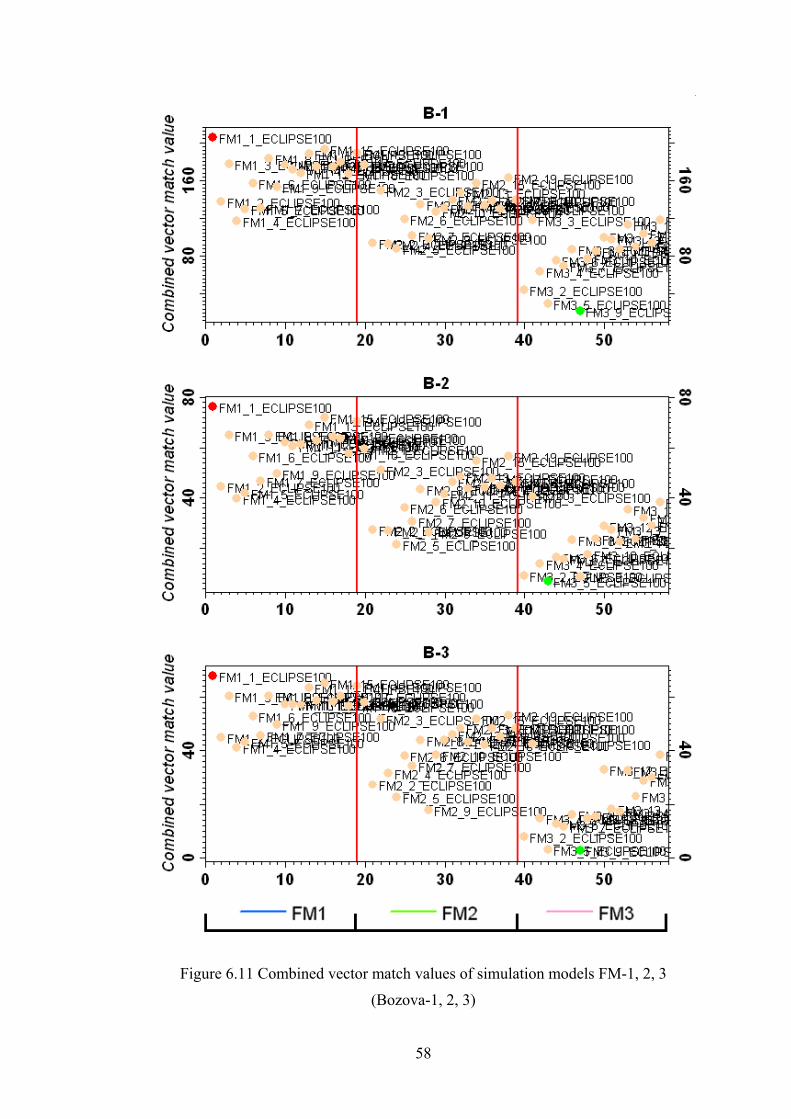
58
Figure 6.11 Combined vector match values of simulation models FM-1, 2, 3
(Bozova-1, 2, 3)

59
Figure 6.12 Combined vector match values of simulation models FM-1, 2, 3
(Bozova-8, 9, Field)

60
Figure 6.13 Combined vector match values of simulation models FM-4, 5, 6
(Bozova-1, 2, 3)

61
Figure 6.14 Combined vector match values of simulation models FM-4, 5, 6
(Bozova-8, 9, Field)

62
Table 6.1 shows the simulation models ranked according to their goodness of fit. The
smallest match values show the best fit models.
Table 6.1 Ranking simulation models according to their match values
Rank Case Combined Vector Rank Case Combined Vector Rank Case Combined VectorOrder Name Match Value Order Name Match Value Order Name Match Value
1 FM3_9 12 39 FM6_17 56 77 FM4_9 782 FM3_5 17 40 FM6_12 57 78 FM5_13 793 FM3_2 24 41 FM6_13 57 79 FM2_13 814 FM6_5 28 42 FM3_15 61 80 FM4_12 815 FM6_9 31 43 FM4_7 63 81 FM4_18 816 FM6_2 32 44 FM1_4 64 82 FM2_3 827 FM3_4 34 45 FM3_19 64 83 FM5_15 838 FM6_4 36 46 FM2_6 65 84 FM5_19 839 FM3_7 37 47 FM4_5 65 85 FM1_9 8410 FM3_6 40 48 FM5_6 65 86 FM4_11 8411 FM6_7 40 49 FM6_3 65 87 FM1_6 8612 FM3_10 41 50 FM6_15 65 88 FM2_15 8613 FM6_6 45 51 FM3_3 66 89 FM4_3 8614 FM6_10 45 52 FM4_2 67 90 FM4_14 8615 FM3_11 46 53 FM5_10 68 91 FM4_16 8616 FM2_5 47 54 FM5_18 68 92 FM4_10 8717 FM3_8 47 55 FM6_19 68 93 FM4_17 8818 FM3_14 47 56 FM2_10 70 94 FM5_1 8919 FM5_5 48 57 FM5_11 70 95 FM4_8 9020 FM3_16 49 58 FM1_5 71 96 FM1_18 9121 FM5_2 49 59 FM1_7 72 97 FM2_19 9122 FM5_4 49 60 FM2_11 72 98 FM4_19 9123 FM2_2 51 61 FM2_18 72 99 FM1_12 9224 FM2_4 51 62 FM5_8 72 100 FM1_11 9425 FM6_8 51 63 FM5_12 72 101 FM4_13 9426 FM6_11 51 64 FM5_14 72 102 FM4_15 9427 FM6_14 51 65 FM5_16 72 103 FM1_14 9628 FM3_18 52 66 FM5_17 72 104 FM1_16 9629 FM6_18 52 67 FM2_14 73 105 FM2_1 9630 FM5_9 53 68 FM2_16 73 106 FM1_3 9731 FM6_16 53 69 FM2_8 74 107 FM1_10 9732 FM2_9 54 70 FM6_1 74 108 FM1_17 9833 FM3_13 54 71 FM1_2 75 109 FM1_8 10134 FM3_12 55 72 FM2_12 76 110 FM4_1 10135 FM5_7 55 73 FM2_17 77 111 FM1_13 10336 FM2_7 56 74 FM3_1 77 112 FM1_19 10337 FM3_17 56 75 FM4_6 77 113 FM1_15 10638 FM4_4 56 76 FM5_3 77 114 FM1_1 113

63
6.2.2 Simulation and History Match Value Results of the 3 Best Cases
The 3 best and the worst matching cases for each well and the field; their corres-
ponding combined vector match values are given Table 6.2.
Table 6.2 The 3 best and the worst matching cases and match values for each well
Case# Value Case# Value Case# Value Case# ValueBozova-1 FM3_9 21 FM3_5 29 FM3_2 43 FM1_1 205Bozova-2 FM3_5 7 FM3_9 9 FM3_2 9 FM1_1 76Bozova-3 FM3_9 3 FM3_5 3 FM3_2 8 FM1_1 68Bozova-8 FM3_9 13 FM3_5 21 FM6_5 25 FM1_1 73Bozova-9 FM1_7 3 FM3_7 3 FM4_4 3 FM2_16 4Field FM3_9 12 FM3_5 17 FM3_2 24 FM1_1 113
Best 2nd Best 3rd Best WorstMatches
Well/Field
Identifying the 3 Best Cases as FM3_9, FM3_5 and FM3_2, their simulation results
are given in the following figures (from Figure 6.15 to Figure 6.20) to see more
clearly.

64
Figure 6.15 Simulation results and vector match values of B-1 for the 3 Best Cases

65
Figure 6.16 Simulation results and vector match values of B-2 for the 3 Best Cases
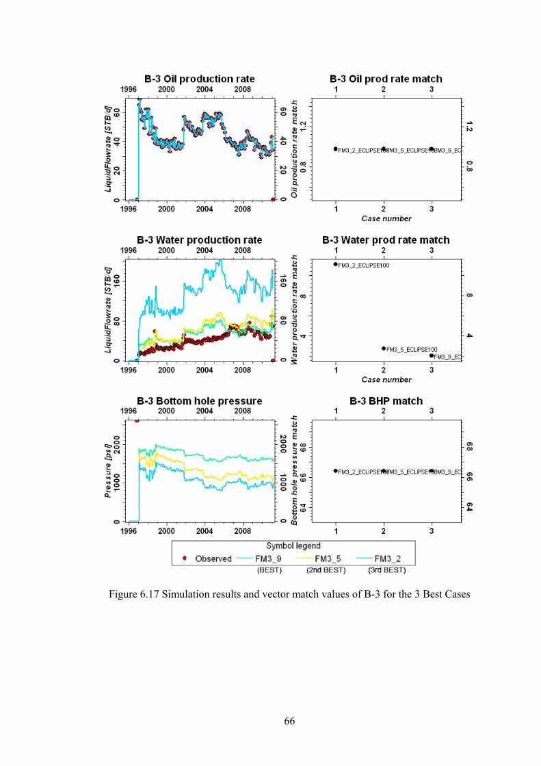
66
Figure 6.17 Simulation results and vector match values of B-3 for the 3 Best Cases

67
Figure 6.18 Simulation results and vector match values of B-8 for the 3 Best Cases

68
Figure 6.19 Simulation results and vector match values of B-9 for the 3 Best Cases

69
Figure 6.20 Simulation results and vector match values of the field for the 3 Best Cases

70
All of the 3 Best Case models have a WOC depth of 1480 m ssTVD, and PVT data
of Bozova-1. The only different items defined in these models are the Pc/krel curves.
Pc/krel curve#9, #5 and #2 belong to plugs named as Boz-2_2, Boz-1_201 and Boz-
1_197 respectively. When investigated through the entire Pc/krel curve sets, these
curves are not the ones with the lowest Swir values. The end points of krw and kro
curves do not give a distinction either. When plotted again, but these 3 best matching
Pc/krel curves in yellow color this time (Figure 6.21), one thing draws the attention
immediately: The similarity on their threshold capillary pressure (Pc threshold)
values being very small. This condition makes the initial water saturation distribution
of the model lower than the ones created with the higher Pc threshold curves; thus
favoring the simulation models. The reason for these 3 curves matching best is not
only the effect of Pc threshold. The krel curves, assigning the fundamental rules of
flow functions, are also of vital importance.
0
200
400
600
800
1000
1200
1400
0 0.2 0.4 0.6 0.8 1
PcL
AB
, p
si
Sw
Boz-1_196Boz-1_198Boz-1_200Boz-1_205Boz-1_206Boz-2_1Boz-2_3Boz-2_4Boz-2_6Boz-2_7Boz-3_266Boz-3_267Boz-3_270Boz-3_272Boz-3_273Boz-3_275Boz-3_286Boz-3_288Boz-3_292Boz-3_294Boz-3_297Boz-3_298Boz-1_201Boz-1_197Boz-2_2
Figure 6.21 Capillary pressure curves emphasizing the 3 best matching curves
The following figure (Figure 6.22) illustrates the match statistics for all wells for the
best case (FM3_9) in the map view. The illustrations show the match values in a
qualitative perspective, the results are lumped into five categories from “Match” to

71
“Poor”. The bigger the bubbles, the bigger the match values, thus the smaller bubbles
show the better matches.
Figure 6.22 Qualitative vector match map for the best case FM3_9
The main issue defining the high match values can be explained by the aquifer
support defined to compensate the high percentage water production of Bozova-2.
When the aquifer provides the high water production and pressure support as ex-
pected in Bozova-2; the water productions of wells Bozova-1, 3 and 8 get worse
(resulting in higher water percentages than observed). The solution should be in a
way that, while Bozova-1, 3 and 8 get pressure support slowly, Bozova-2 should be
in a more direct interaction with the aquifer. A comparative study on the strength of
aquifer, the connection area of aquifer, permeability model, kh/kv ratio and krel
curves can help working on this problem.

72
6.3 Uncertainty Quantification Results
Quantification of uncertainty is obtained by following two different evaluation
methods. The first method aims to calculate the impact of each variable on each
vector match, and to determine the variable whose uncertainty affects the results the
most. The second method’s objective is the determination of impact of uncertainties
only on STOOIP values of the resulting cases. Briefly, the first method provides the
impact of uncertainty on dynamic results; whereas the second method focuses on
static results of the simulation models.
6.3.1 Uncertainty Quantification by Using History Match Statistics
In order to quantify the impact of uncertainty of each variable, i.e., PVT, WOC and
Pc/krel, history match values of the cases are compared in a systematic way. The
cases are grouped into classes so that the variable of interest, the uncertainty impact
of which is to be investigated, is varied and the remaining variables are kept con-
stant. In each group, regarding the combined and each individual vector separately, a
best and a worst matching case is selected. After that, the history match values of
these cases are tabulated. The differences between the match values represent the
range of effect the variable can create on the result. By this way, the uncertainty
impact of each variable on each vector match is calculated, and the variable uncer-
tainty which affects the results the most is determined.
In order to calculate the impact of PVT data uncertainty, 6 classes are formed so that
in each class the only changing variable is PVT data. The first table in Table 6.3
belongs to simulation cases with a WOC depth of 1455 m ssTVD and Pc/krel
curve#1. Since forming classes for 19 Pc/krel curve sets is tedious; the curves are
decreased to 2 representative sets. As Pc/krel curves is not a single numeric value to
be determined as minimum and maximum, the most and least matching curves with
the results are chosen as Pc/krel curve#1 and #9. In each class, the difference of
match value between the best and worst case is calculated as range of effect, which
corresponds only to the impact of uncertainty that belongs to the changed variable.
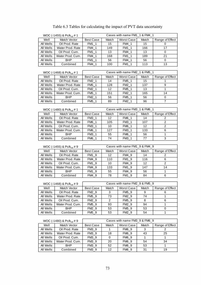
73
Table 6.3 Tables for calculating the impact of PVT data uncertainty
Well Match Vector Best Case Match Worst Case Match Range of EffectAll Wells Oil Prod. Rate FM1_1 15 FM4_1 15 0All Wells Water Prod. Rate FM4_1 149 FM1_1 166 17All Wells Oil Prod. Cum. FM1_1 13 FM4_1 13 0All Wells Water Prod. Cum. FM4_1 168 FM1_1 189 21All Wells BHP FM1_1 56 FM4_1 56 0All Wells Combined FM4_1 100 FM1_1 113 13
Well Match Vector Best Case Match Worst Case Match Range of EffectAll Wells Oil Prod. Rate FM2_1 14 FM5_1 15 1All Wells Water Prod. Rate FM5_1 128 FM2_1 137 9All Wells Oil Prod. Cum. FM2_1 12 FM5_1 13 1All Wells Water Prod. Cum. FM5_1 151 FM2_1 165 14All Wells BHP FM2_1 56 FM5_1 56 0All Wells Combined FM5_1 89 FM2_1 96 7
Well Match Vector Best Case Match Worst Case Match Range of EffectAll Wells Oil Prod. Rate FM3_1 12 FM6_1 14 2All Wells Water Prod. Rate FM6_1 105 FM3_1 107 2All Wells Oil Prod. Cum. FM3_1 10 FM6_1 12 2All Wells Water Prod. Cum. FM6_1 127 FM3_1 133 6All Wells BHP FM3_1 55 FM6_1 56 1All Wells Combined FM6_1 74 FM3_1 77 3
Well Match Vector Best Case Match Worst Case Match Range of EffectAll Wells Oil Prod. Rate FM1_9 12 FM4_9 14 2All Wells Water Prod. Rate FM4_9 110 FM1_9 116 6All Wells Oil Prod. Cum. FM1_9 10 FM4_9 12 2All Wells Water Prod. Cum. FM4_9 133 FM1_9 147 14All Wells BHP FM1_9 55 FM4_9 56 1All Wells Combined FM4_9 78 FM1_9 84 6
Well Match Vector Best Case Match Worst Case Match Range of EffectAll Wells Oil Prod. Rate FM2_9 3 FM5_9 9 6All Wells Water Prod. Rate FM5_9 73 FM2_9 74 1All Wells Oil Prod. Cum. FM2_9 2 FM5_9 8 6All Wells Water Prod. Cum. FM5_9 93 FM2_9 94 1All Wells BHP FM2_9 53 FM5_9 53 0All Wells Combined FM5_9 53 FM2_9 54 1
Well Match Vector Best Case Match Worst Case Match Range of EffectAll Wells Oil Prod. Rate FM3_9 1 FM6_9 3 2All Wells Water Prod. Rate FM3_9 18 FM6_9 43 25All Wells Oil Prod. Cum. FM3_9 0 FM6_9 1 1All Wells Water Prod. Cum. FM3_9 20 FM6_9 54 34All Wells BHP FM3_9 52 FM6_9 53 1All Wells Combined FM3_9 12 FM6_9 31 19
WOC (-1480) & Pc/krel # 9 Cases with name FM3_9 & FM6_9
WOC (-1468) & Pc/krel # 1 Cases with name FM2_1 & FM5_1
WOC (-1480) & Pc/krel # 1 Cases with name FM3_1 & FM6_1
WOC (-1455) & Pc/krel # 9 Cases with name FM1_9 & FM4_9
WOC (-1468) & Pc/krel # 9 Cases with name FM2_9 & FM5_9
Cases with name FM1_1 & FM4_1WOC (-1455) & Pc/krel # 1

74
The same procedure is followed for calculating the impacts of uncertainties that
belong to WOC depth and Pc/krel curves. The tables created for the calculations are
given in Table 6.4 and Table 6.5. In Table 6.4, variables other than WOC depth
(PVT, Pc/krel) are kept constant in each class, whereas variables other than Pc/krel
curve (PVT, WOC) are kept constant in Table 6.5.
Table 6.4 Tables for calculating the impact of WOC depth uncertainty
Well Match Vector Best Case Match Worst Case Match Range of EffectAll Wells Oil Prod. Rate FM3_1 12 FM1_1 15 3All Wells Water Prod. Rate FM3_1 107 FM1_1 166 59All Wells Oil Prod. Cum. FM3_1 10 FM1_1 13 3All Wells Water Prod. Cum. FM3_1 133 FM1_1 189 56All Wells BHP FM3_1 55 FM1_1 56 1All Wells Combined FM3_1 77 FM1_1 113 36
Well Match Vector Best Case Match Worst Case Match Range of EffectAll Wells Oil Prod. Rate FM6_1 14 FM4_1 15 1All Wells Water Prod. Rate FM6_1 105 FM4_1 149 44All Wells Oil Prod. Cum. FM6_1 12 FM4_1 13 1All Wells Water Prod. Cum. FM6_1 127 FM4_1 168 41All Wells BHP FM6_1 56 FM4_1 56 0All Wells Combined FM6_1 74 FM4_1 101 27
Well Match Vector Best Case Match Worst Case Match Range of EffectAll Wells Oil Prod. Rate FM3_9 1 FM1_9 12 11All Wells Water Prod. Rate FM3_9 18 FM1_9 116 98All Wells Oil Prod. Cum. FM3_9 0 FM1_9 10 10All Wells Water Prod. Cum. FM3_9 20 FM1_9 147 127All Wells BHP FM3_9 52 FM1_9 55 3All Wells Combined FM3_9 12 FM1_9 84 72
Well Match Vector Best Case Match Worst Case Match Range of EffectAll Wells Oil Prod. Rate FM6_9 3 FM4_9 14 11All Wells Water Prod. Rate FM6_9 43 FM4_9 110 67All Wells Oil Prod. Cum. FM6_9 1 FM4_9 12 11All Wells Water Prod. Cum. FM6_9 54 FM4_9 133 79All Wells BHP FM6_9 52 FM4_9 56 4All Wells Combined FM6_9 31 FM4_9 78 47
PVT-3 & Pc/krel # 9 Cases with name FM4_9 & FM5_9 & FM6_9
PVT-1 & Pc/krel # 1 Cases with name FM1_1 & FM2_1 & FM3_1
PVT-3 & Pc/krel # 1 Cases with name FM4_1 & FM5_1 & FM6_1
PVT-1 & Pc/krel # 9 Cases with name FM1_9 & FM2_9 & FM3_9
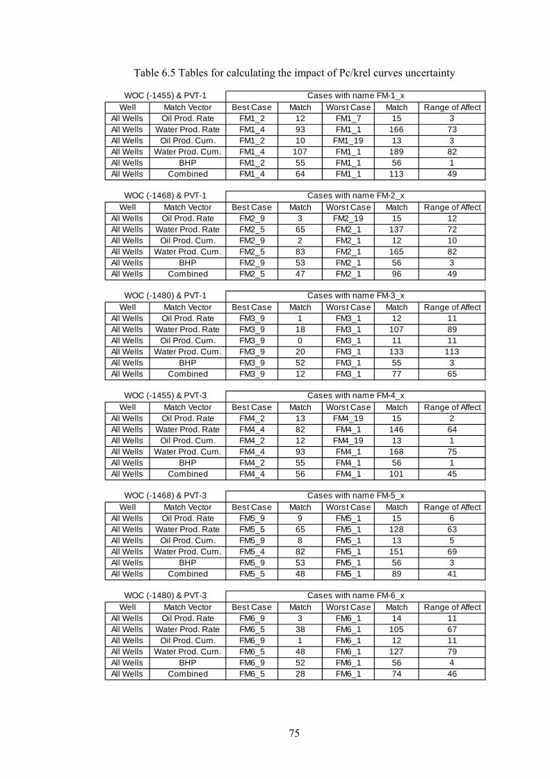
75
Table 6.5 Tables for calculating the impact of Pc/krel curves uncertainty
Well Match Vector Best Case Match Worst Case Match Range of AffectAll Wells Oil Prod. Rate FM1_2 12 FM1_7 15 3All Wells Water Prod. Rate FM1_4 93 FM1_1 166 73All Wells Oil Prod. Cum. FM1_2 10 FM1_19 13 3All Wells Water Prod. Cum. FM1_4 107 FM1_1 189 82All Wells BHP FM1_2 55 FM1_1 56 1All Wells Combined FM1_4 64 FM1_1 113 49
Well Match Vector Best Case Match Worst Case Match Range of AffectAll Wells Oil Prod. Rate FM2_9 3 FM2_19 15 12All Wells Water Prod. Rate FM2_5 65 FM2_1 137 72All Wells Oil Prod. Cum. FM2_9 2 FM2_1 12 10All Wells Water Prod. Cum. FM2_5 83 FM2_1 165 82All Wells BHP FM2_9 53 FM2_1 56 3All Wells Combined FM2_5 47 FM2_1 96 49
Well Match Vector Best Case Match Worst Case Match Range of AffectAll Wells Oil Prod. Rate FM3_9 1 FM3_1 12 11All Wells Water Prod. Rate FM3_9 18 FM3_1 107 89All Wells Oil Prod. Cum. FM3_9 0 FM3_1 11 11All Wells Water Prod. Cum. FM3_9 20 FM3_1 133 113All Wells BHP FM3_9 52 FM3_1 55 3All Wells Combined FM3_9 12 FM3_1 77 65
Well Match Vector Best Case Match Worst Case Match Range of AffectAll Wells Oil Prod. Rate FM4_2 13 FM4_19 15 2All Wells Water Prod. Rate FM4_4 82 FM4_1 146 64All Wells Oil Prod. Cum. FM4_2 12 FM4_19 13 1All Wells Water Prod. Cum. FM4_4 93 FM4_1 168 75All Wells BHP FM4_2 55 FM4_1 56 1All Wells Combined FM4_4 56 FM4_1 101 45
Well Match Vector Best Case Match Worst Case Match Range of AffectAll Wells Oil Prod. Rate FM5_9 9 FM5_1 15 6All Wells Water Prod. Rate FM5_5 65 FM5_1 128 63All Wells Oil Prod. Cum. FM5_9 8 FM5_1 13 5All Wells Water Prod. Cum. FM5_4 82 FM5_1 151 69All Wells BHP FM5_9 53 FM5_1 56 3All Wells Combined FM5_5 48 FM5_1 89 41
Well Match Vector Best Case Match Worst Case Match Range of AffectAll Wells Oil Prod. Rate FM6_9 3 FM6_1 14 11All Wells Water Prod. Rate FM6_5 38 FM6_1 105 67All Wells Oil Prod. Cum. FM6_9 1 FM6_1 12 11All Wells Water Prod. Cum. FM6_5 48 FM6_1 127 79All Wells BHP FM6_9 52 FM6_1 56 4All Wells Combined FM6_5 28 FM6_1 74 46
WOC (-1455) & PVT-3 Cases with name FM-4_x
WOC (-1468) & PVT-3 Cases with name FM-5_x
WOC (-1480) & PVT-3 Cases with name FM-6_x
WOC (-1455) & PVT-1 Cases with name FM-1_x
WOC (-1468) & PVT-1 Cases with name FM-2_x
WOC (-1480) & PVT-1 Cases with name FM-3_x

76
So as to see the overall effects more clearly, to see the big picture, the ranges of
effects of each class are averaged and are shown in Table 6.6.
Table 6.6 Impact of PVT, WOC, Pc/krel uncertainty on different vector matches
Well Match Vector PVT WOC PC/KRELAll Wells Oil Prod. Rate 2 7 8All Wells Water Prod. Rate 10 67 71All Wells Oil Prod. Cum. 2 6 7All Wells Water Prod. Cum. 15 76 83All Wells BHP 1 2 3All Wells Combined 8 46 49
AVG. RANGE OF EFFECT OF
The table demonstrates that PVT data do not seem to noticeably impact the match
results when compared to the impact of WOC depth and Pc/krel curve data. The two
most dominantly affecting variables, the uncertainty impacts of which are seen on all
vector matches (both individually and combined), are Pc/krel and WOC depth data.
Inspecting the Pc/krel uncertainty, due to the fact that it is responsible of the water
breakthrough time, its impact, is mostly related to water production rate and water
production cumulative results. Following it, impacts on oil production rate and oil
production cumulative results comes next with much smaller range of effect values.
With close range of effect values, defining the reasons of high water production by a
direct relation, impact of WOC uncertainty comes next.
Searching on BHP matches, the effect of Pc/krel and WOC shares the first two rows
as the variables having the highest impact, but they are not as determinant as they are
on production matches.
6.3.2 Uncertainty Quantification by Two Level (2k) Factorial Design Technique
In this study, in order to investigate the effects of Pc/krel, PVT and WOC on
STOOIP values, a two level design is constructed and analyzed.

77
As explained in detail in “5.5 Two Level (2k) Factorial Design Technique as an
Uncertainty Quantification Method”, the 23 factorial design technique is applied in
order to quantify the impact of uncertainties on STOOIP values. The coded and
uncoded design matrix is as given in Table 6.7. The geometrical representation of the
23 design is given in Figure 6.23.
Table 6.7 Coded and uncoded factorial design with results
Test Run No x1 x2 x3 PC & KREL WOC PVT y (STOOIP) CASE#1 -1 -1 -1 MIN -1455 PVT-3 3,762,259 FM4_192 +1 -1 -1 MAX -1455 PVT-3 15,411,842 FM4_173 -1 +1 -1 MIN -1480 PVT-3 17,238,416 FM6_194 +1 +1 -1 MAX -1480 PVT-3 37,429,903 FM6_25 -1 -1 +1 MIN -1455 PVT-1 5,031,518 FM1_196 +1 -1 +1 MAX -1455 PVT-1 15,412,913 FM1_177 -1 +1 +1 MIN -1480 PVT-1 20,899,394 FM3_198 +1 +1 +1 MAX -1480 PVT-1 38,575,917 FM3_2
DESIGN MATRIX CODED DESIGN MATRIX UNCODED
Figure 6.23 Geometrical representation of the 23 design
By using the simplified method average effects, two-factor and three-factor interac-
tions are calculated as follows:
E1 (Average effect of PC & Krel) = 14,974,747
E2 (Average effect of WOC) = 18,631,275

78
E3 (Average effect of PVT) = 1,519,331
E12 (Interaction of PC & Krel and WOC) = 3,959,258
E13 (Interaction of PC & Krel and PVT) = -945,788
E23 (Interaction of WOC and PVT) = 884,166
E123 (Interaction of PC & Krel, WOC and PVT) = -311,694
The analysis of the results is carried out by ranking the effects and interactions
according to the absolute magnitudes and given in Table 6.8
Table 6.8 Ranking the average effects on STOOIP
Average Effect on STOOIPWOC 18.6 x 10⁶
Pc/krel 15 x 106
WOC & Pc/krel 4 x 10⁶
PVT 1.5 x 10⁶
Pc/krel & PVT 0.95 x 10⁶
WOC & PVT 0.88 x 10⁶
WOC & Pc/krel & PVT 0.31 x 10⁶
When the issue is the determination of STOOIP, the ranking indicates that WOC is
the most important variable and Pc/krel effect follows it with a close magnitude of
effect. It is also seen that the interaction of WOC and Pc/krel is bigger than the
average effect of PVT alone. One should not confuse the interaction with the sum of
the effects. The interaction, as the name implies, refers only to the effect that arises
from the combination of two items, the results of which are not independent of each
other. The remaining two and three factor interactions show that PVT data is quite
independent of WOC and Pc/krel.

79
CHAPTER 7
CONCLUSIONS
This study emphasizes that the uncertainties of dynamic reservoir properties should
be given as much attention as the uncertainty of static reservoir properties when
modeling an accurate reservoir simulation.
When the results of the simulations are visualized, it is clearly seen that, the domi-
nant factor that affects the match for production rates is the fluid model. Fluid model
is constructed upon combination of 2 items; WOC and PVT properties. Screening
results do not clarify whether WOC depth is or Pc/krel curves are more determinant
on the production rate results.
Screening indicates that, simulation cases of FM3, FM6 (having a WOC of 1480 m
ssTVD), are the best matched models. Also FM2 (having a WOC of 1468 m
ssTVD), shows matched results for some of the wells. The worst matched simulation
models FM1 and FM4 are not capable of producing the target oil production rates
even if they produce too much water. The goodness of the water production rate
results is parallel to the goodness of the oil production rate results in that, as the
water production rate results get closer to the observed data, oil production rate
results also get closer to the observed data.
The 3 Best Case models are identified and they all have a WOC depth of 1480 m
ssTVD, and PVT data of Bozova-1. The only different items defined in these models
are the Pc/krel curves. The similarity on their Pc threshold values being very small,
makes the Swi distribution of the model lower than the ones created with the higher
Pc threshold curves; thus favoring the simulation models. The reason for these 3
curves matching best is not only the effect of Pc threshold. The krel curves, assign-
ing the fundamental rules of flow functions, are also of vital importance.

80
Regarding the range of effects the variables can create on the dynamic simulation
results, the uncertainty impact of Pc/krel curves is the most affecting variable; the
uncertainty of WOC follows it with a close range of effect; and the least effect arises
from the uncertainty of PVT data.
When the issue is the determination of STOOIP, it is found that WOC is the most
important variable and Pc/krel follows it with a close magnitude of effect. It is also
seen that the interaction of WOC and Pc/krel is bigger than the average effect of
PVT alone.

81
CHAPTER 8
RECOMMENDATIONS
Based on the achieved simulation results, there are a number of considerations that
must be taken into account in future studies, especially for the history matching
process. In addition to the uncertain parameters that are taken into account, parame-
ters such as aquifer strength, aquifer connection area, aquifer influx; kv/kh ratio;
permeability model; and Pc/krel curves other than the experimental data should also
be considered. As the number of uncertain parameters gets larger, the number of
simulation results required also gets larger. Therefore, building a proxy model which
connects the results to all influent uncertain parameters may help a more effective
uncertainty analysis. In order to identify the actually influent parameters, fractional
factorial designs may be used rather than the full factorial experimental designs.

82
REFERENCES
Al-Shamma, B.R., Teigland, R., 2006, “History Matching of the Valhall Field Using
a Global Optimization Method and Uncertainty Assessment”, SPE 100946, Pre-
sented at the 2006 SPE Annual Technical Conference and Exhibition held in San
Antonio, Texas, U.S.A., 24-27 September 2006.
Capen, E.C., 1975, “The Difficulty of Assessing Uncertainty”, SPE 5579, Presented
at the 1975 SPE-AIME Annual Technical Conference and Exhibition, Dallas, 28
September-1 October 1975.
Çalışgan., H., 1996, “PVT Analysis Report of Bozova-1 Reservoir Oil”, Report No
2148, TPAO, Research Center, Reservoir Management, March 1996.
Çalışgan., H., 1996, “PVT Analysis Report of Bozova-3 Reservoir Oil”, Report No
2236, TPAO, Research Center, Reservoir Management, February 1997.
Dejean, J.P., Blanc, G.,1999, “Managing Uncertainties on Production Predictions
Using Integrated Statistical Methods”, SPE 56696, Presented at the 1999 Annual
Technical Conference and Exhibition held in Houston, Texas, 3-6 October 1999.
Evin, S., Soyhan, N., 2002, “Reservoir Evaluation Study of Bozova Field”, Technic-
al Report, TPAO, Production Department, Reservoir Management, June 2002.
Ferno, M.A., Treinen R., and Graue, A., 2007, “Experimental Measurements of
Capillary Pressure with the Centrifuge Technique – Emphasis on Equilibrium Time
and Accuracy in Production”, SCA2007-22, Presented at the International Sympo-
sium of the Society of Core Analysts Calgary, Canada, 10-12 September 2007.

83
Hajizadeh, Y., Christie, M., Demyanov, V., 2009, “Ant Colony Optimization for
History Matching”, SPE 121193, Presented at the 2009 SPE EUROPEC/EAGE
Annual Conference and Exhibition held in Amsterdam, The Netherlands, 8-11 June
2009.
Holmes, M., 2002, “Capillary Pressure & Relative Permeability Petrophysical
Reservoir Models”, Technical Report of Digital Formation Inc., Denver, Colorado,
U.S.A., 2002.
Karabakal, U., 1998, “Conventional and Special Core Analysis Report of Wells
Bozova-1, 2 and 3”, Report No 2323, TPAO, Research Center, Reservoir Manage-
ment, March 1998.
Karakeçe, Y., 1999 “Log Process of Bozova Wells”, TPAO, Production Department,
Reservoir Management, 1999.
Leuangthong, O., Deutsch, C.V., 2003, “Experimental Design Matrix of Realizations
for Optimal Sensitivity Analysis”, Technical report, Centre of Computational
Geostatistics, University of Alberta, Edmonton, AB, September 2003.
Li, K., Horne, R. N., 2003, “Numerical Simulation with Input Consistency between
Capillary Pressure and Relative Permeability”, SPE 79716 presented at the SPE
Reservoir Simulation Symposium held in Houston, Texas, U.S. A., 3-5 February
2003.
Manceau, E., Mezghani, M., Zabalza-Mezghani, I., Roggero, F., 2001, “Combination
of Experimental Design and Joint Modeling Methods for Quantifying the Risk
Associated with Deterministic and Stochastic Uncertainties – An Integrated Test
Study”, SPE 71620, Presented at the 2001 SPE Annual Technical Conference and
Exhibition held in New Orleans, Louisiana, U.S.A., 30 September-3 October 2001.
Mogford, M., 2007, “Introduction to Relative Permeability”, Presented at the AFES
Meeting, Aberdeen, 28 March 2007.

84
Mohammed, L., Christie, M., Demyanov, V., 2009, “Comparison of Stochastic
Sampling Algorithms for Uncertainty Quantification”, SPE 119139, Presented at the
2009 SPE Reservoir Simulation Symposium, The Woodlands, Texas, U.S.A., 2-4
February 2009.
Peterson, R.D., Yawanarah, S., Neisch, D., Tabanou E., and James, S., 2006, “To-
wards a Framework for Better Decision Making under Subsurface Uncertainty”, SPE
99484, presented at the 2006 Intelligent Energy Conference and Exhibition held in
Amsterdam, The Netherlands, 11-13 April 2006.
Potlog, S., 2003, "Uncertainty Quantification and Risk Analysis for Petroleum
Exploration and Exploitation Projects", Department of Civil & Environmental
Engineering, University of Alberta, 2003.
Rotondi, M., Nicotra, G., Godi, A., Contento, F.M., Blunt, M.J., Christie, M.A.,
2006, "Hydrocarbon Production Forecast and Uncertainty Quantification: A Field
Application", SPE 102135, Presented at the 2006 SPE Annual Technical Conference
and Exhibition held in San Antonio, Texas, U.S.A.,24-27 September 2006.
Salarieh, M., Doroudi, A., Sobhi, G.A., and Bashiri, G.R., 2004, “The Role of
Capillary Pressure Curves in Reservoir Simulation Studies”, Technical Report,
Research Institute of Petroleum Industry.
Salomão, M.C., and Grell, A.P., 2001. "Uncertainty in Production Profiles on the
Basis of Geostatistic Characterization and Flow Simulation", paper SPE 69477,
Presented at the SPE Latin American and Caribbean Petroleum Engineering Confe-
rence held in Buenos Aires, Argentina, 25–28 March 2001.
Saxena, U., Pavelic, V., 1971, “Factorial Designs as an Effective Tool in Mining and
Petroleum Engineering”, SPE 3333, Society of Petroleum Engineers Journal, 1971.
Şengündüz, N., Çoruh, T., İlleez, H., Karabakal, U., and Selvi, B., 2000, “XII. Bölge
Bozova, Suvarlı, Araban Sahaları ve Civarının Jeolojik Değerlendirmesi”, Technical
Report, TPAO, Research Department, 2000.

85
Venkatamaran, R., 2000. “Application of the Method of Experimental Design to
Quantify Uncertainty in Production Profiles”, SPE 59422, presented at the 2000 SPE
Asia Pacific Conference on Integrated Modeling for Asset Management held in
Yokohama, Japan, 25-26 April 2000.
Zabalza-Mezghani, I., Manceau, E., Feraille, M., and Jourdan, A., 2004. "Uncertain-
ty Management: From Geological Scenarios to Production Scheme Optimization",
Journal of Petroleum Science and Engineering 44, 11-25, 2004.
Zabel, F., Law, D.H.S., Taylor, S., Zuo, J., 2008. “Impact of Uncertainty of Heavy
Oil Fluid Property Measurement”, Proceedings of the Canadian International Petro-
leum Conference/SPE Gas Technology Symposium 2008 Joint Conference, Canada,
2008.
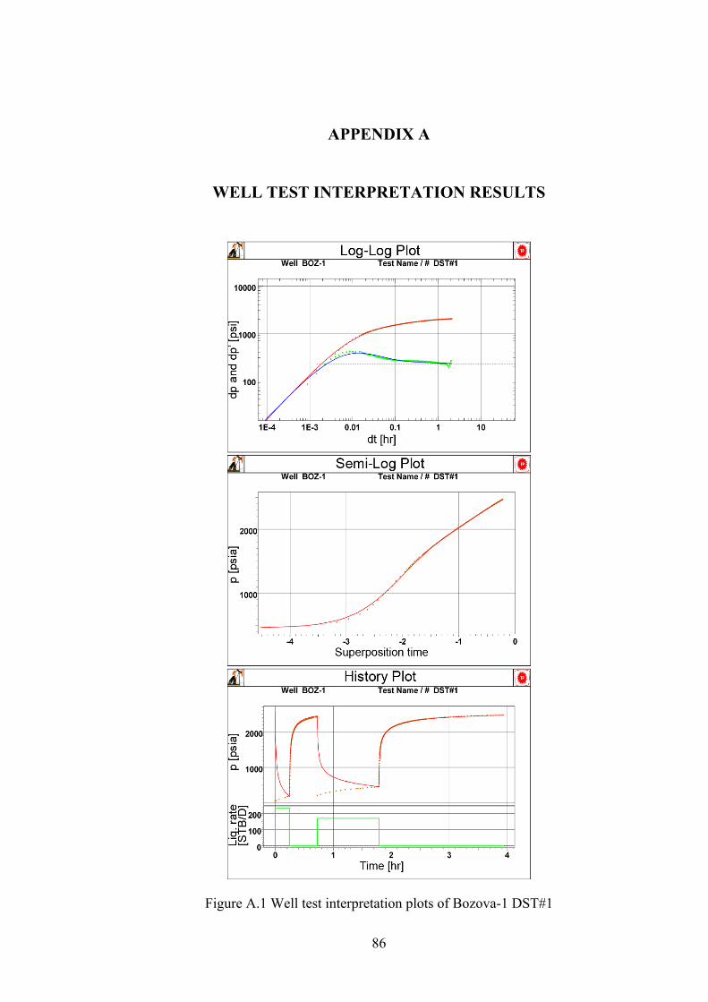
86
APPENDIX A
WELL TEST INTERPRETATION RESULTS
Figure A.1 Well test interpretation plots of Bozova-1 DST#1
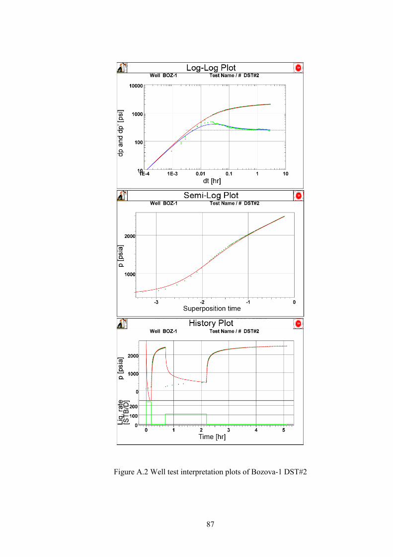
87
Figure A.2 Well test interpretation plots of Bozova-1 DST#2

88
Figure A.3 Well test interpretation plots of Bozova-2 DST#1

89
Figure A.4 Well test interpretation plots of Bozova-2 DST#2
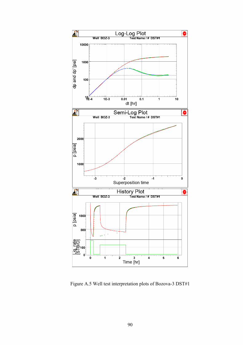
90
Figure A.5 Well test interpretation plots of Bozova-3 DST#1
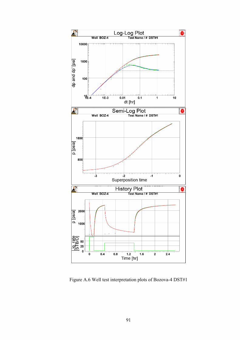
91
Figure A.6 Well test interpretation plots of Bozova-4 DST#1

92
Figure A.7 Well test interpretation plots of Bozova-4 DST#2

93
Figure A.8 Well test interpretation plots of Bozova-5 DST#1

94
Figure A.9 Well test interpretation plots of Bozova-8 DST#1

95
Figure A.10 Well test interpretation plots of Bozova-9 DST#1
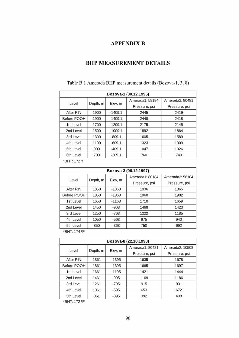
96
APPENDIX B
BHP MEASUREMENT DETAILS
Table B.1 Amerada BHP measurement details (Bozova-1, 3, 8)
Amerada1: 58184 Amerada2: 80481Pressure, psi Pressure, psi
After RIN 1900 -1409.1 2445 2419Before POOH 1900 -1409.1 2448 2418
1st Level 1700 -1209.1 2175 21452nd Level 1500 -1009.1 1892 18643rd Level 1300 -809.1 1605 15894th Level 1100 -609.1 1323 13095th Level 900 -409.1 1047 10266th Level 700 -209.1 760 740
*BHT: 172 ºF
Amerada1: 80184 Amerada2: 58184Pressure, psi Pressure, psi
After RIN 1850 -1363 1936 1865Before POOH 1850 -1363 1960 1902
1st Level 1650 -1163 1710 16592nd Level 1450 -963 1468 14233rd Level 1250 -763 1222 11854th Level 1050 -563 975 9405th Level 850 -363 750 692
*BHT: 174 ºF
Amerada1: 80481 Amerada2: 10508Pressure, psi Pressure, psi
After RIN 1861 -1395 1635 1678Before POOH 1861 -1395 1665 1697
1st Level 1661 -1195 1421 14442nd Level 1461 -995 1169 11863rd Level 1261 -795 915 9314th Level 1061 -595 653 6725th Level 861 -395 392 408
*BHT: 172 ºF
Bozova-8 (22.10.1998)
Level Depth, m Elev, m
Bozova-1 (30.12.1995)
Level Depth, m Elev, m
Bozova-3 (06.12.1997)
Level Depth, m Elev, m

97
Figure B.1 Pressure vs. depth plots of Amerada BHP measurements (Bozova-1, 3, 8)

98
Table B.2 Spartek BHP measurement details (Bozova-2, 8, 9)
Spartek-1197Pressure, psi
Before POOH 1335 -852 14961st Level 1200 -717 13062nd Level 1000 -517 10243rd Level 800 -317 7414th Level 600 -117 4585th Level 400 83 1786th Level 350 133 111
*BHT: 150 ºF
Spartek-1197Pressure, psi
Before POOH 1700 -1239 13141st Level 1500 -1039 10282nd Level 1300 -839 7413rd Level 1100 -639 4544th Level 900 -439 193
*BHT: 170 ºF
Spartek-1197Pressure, psi
Before POOH 1860 -1400 20171st Level 1700 -1240 17942nd Level 1500 -1040 15143rd Level 1300 -840 12324th Level 1100 -640 9495th Level 900 -440 6836th Level 700 -240 4237th Level 500 -40 164
*BHT: 176 ºF
Bozova-9 (16.02.2011)
Level Depth, m Elev, m
Bozova-2 (15.02.2011)
Level Depth, m Elev, m
Bozova-8 (16.02.2011)
Level Depth, m Elev, m

99
Figure B.2 Pressure vs. depth plots of Spartek BHP measurements (Bozova-2, 8, 9)

100
APPENDIX C
EXPERIMENTAL DESIGN TABLE
Table C.1 Experimental design used for the simulation runs and STOOIP results
CASE# PVT WOC STOOIP CASE# PVT WOC STOOIPFM1_1 PVT-1 -1455 #1 Boz-1_196 13,733,730 FM4_1 PVT-3 -1455 #1 Boz-1_196 13,037,280FM1_2 PVT-1 -1455 #2 Boz-1_197 15,373,053 FM4_2 PVT-3 -1455 #2 Boz-1_197 14,970,914FM1_3 PVT-1 -1455 #3 Boz-1_198 8,372,368 FM4_3 PVT-3 -1455 #3 Boz-1_198 6,988,187FM1_4 PVT-1 -1455 #4 Boz-1_200 8,027,234 FM4_4 PVT-3 -1455 #4 Boz-1_200 6,861,376FM1_5 PVT-1 -1455 #5 Boz-1_201 11,629,868 FM4_5 PVT-3 -1455 #5 Boz-1_201 10,385,157FM1_6 PVT-1 -1455 #6 Boz-1_205 8,327,527 FM4_6 PVT-3 -1455 #6 Boz-1_205 7,011,178FM1_7 PVT-1 -1455 #7 Boz-1_206 6,836,962 FM4_7 PVT-3 -1455 #7 Boz-1_206 5,242,750FM1_8 PVT-1 -1455 #8 Boz-2_1 13,730,676 FM4_8 PVT-3 -1455 #8 Boz-2_1 13,134,543FM1_9 PVT-1 -1455 #9 Boz-2_2 13,935,673 FM4_9 PVT-3 -1455 #9 Boz-2_2 13,174,781FM1_10 PVT-1 -1455 #10 Boz-2_4 10,855,029 FM4_10 PVT-3 -1455 #10 Boz-2_4 10,006,776FM1_11 PVT-1 -1455 #11 Boz-2_6 9,364,930 FM4_11 PVT-3 -1455 #11 Boz-2_6 7,995,004FM1_12 PVT-1 -1455 #12 Boz-3_266 5,921,242 FM4_12 PVT-3 -1455 #12 Boz-3_266 4,689,297FM1_13 PVT-1 -1455 #13 Boz-3_267 7,273,033 FM4_13 PVT-3 -1455 #13 Boz-3_267 6,026,677FM1_14 PVT-1 -1455 #14 Boz-3_272 8,900,736 FM4_14 PVT-3 -1455 #14 Boz-3_272 7,710,688FM1_15 PVT-1 -1455 #15 Boz-3_273 6,974,948 FM4_15 PVT-3 -1455 #15 Boz-3_273 5,617,546FM1_16 PVT-1 -1455 #16 Boz-3_275 8,050,662 FM4_16 PVT-3 -1455 #16 Boz-3_275 6,723,079FM1_17 PVT-1 -1455 #17 Boz-3_288 15,412,913 FM4_17 PVT-3 -1455 #17 Boz-3_288 15,411,842FM1_18 PVT-1 -1455 #18 Boz-3_294 14,608,149 FM4_18 PVT-3 -1455 #18 Boz-3_294 14,472,566FM1_19 PVT-1 -1455 #19 Boz-3_297 5,031,518 FM4_19 PVT-3 -1455 #19 Boz-3_297 3,762,259FM2_1 PVT-1 -1468 #1 Boz-1_196 24,521,611 FM5_1 PVT-3 -1468 #1 Boz-1_196 23,299,621FM2_2 PVT-1 -1468 #2 Boz-1_197 26,489,014 FM5_2 PVT-3 -1468 #2 Boz-1_197 25,672,659FM2_3 PVT-1 -1468 #3 Boz-1_198 17,532,330 FM5_3 PVT-3 -1468 #3 Boz-1_198 15,148,177FM2_4 PVT-1 -1468 #4 Boz-1_200 16,501,478 FM5_4 PVT-3 -1468 #4 Boz-1_200 14,292,736FM2_5 PVT-1 -1468 #5 Boz-1_201 22,462,843 FM5_5 PVT-3 -1468 #5 Boz-1_201 20,387,774FM2_6 PVT-1 -1468 #6 Boz-1_205 17,406,658 FM5_6 PVT-3 -1468 #6 Boz-1_205 14,890,925FM2_7 PVT-1 -1468 #7 Boz-1_206 15,670,385 FM5_7 PVT-3 -1468 #7 Boz-1_206 12,711,197FM2_8 PVT-1 -1468 #8 Boz-2_1 24,346,652 FM5_8 PVT-3 -1468 #8 Boz-2_1 23,138,960FM2_9 PVT-1 -1468 #9 Boz-2_2 25,079,135 FM5_9 PVT-3 -1468 #9 Boz-2_2 23,657,242FM2_10 PVT-1 -1468 #10 Boz-2_4 20,239,824 FM5_10 PVT-3 -1468 #10 Boz-2_4 18,663,111FM2_11 PVT-1 -1468 #11 Boz-2_6 19,126,902 FM5_11 PVT-3 -1468 #11 Boz-2_6 16,769,316FM2_12 PVT-1 -1468 #12 Boz-3_266 13,216,708 FM5_12 PVT-3 -1468 #12 Boz-3_266 10,880,569FM2_13 PVT-1 -1468 #13 Boz-3_267 15,431,811 FM5_13 PVT-3 -1468 #13 Boz-3_267 13,163,922FM2_14 PVT-1 -1468 #14 Boz-3_272 17,946,893 FM5_14 PVT-3 -1468 #14 Boz-3_272 15,792,714FM2_15 PVT-1 -1468 #15 Boz-3_273 15,287,605 FM5_15 PVT-3 -1468 #15 Boz-3_273 12,746,306FM2_16 PVT-1 -1468 #16 Boz-3_275 16,884,159 FM5_16 PVT-3 -1468 #16 Boz-3_275 14,544,029FM2_17 PVT-1 -1468 #17 Boz-3_288 25,652,380 FM5_17 PVT-3 -1468 #17 Boz-3_288 25,297,794FM2_18 PVT-1 -1468 #18 Boz-3_294 24,694,196 FM5_18 PVT-3 -1468 #18 Boz-3_294 24,097,914FM2_19 PVT-1 -1468 #19 Boz-3_297 11,906,167 FM5_19 PVT-3 -1468 #19 Boz-3_297 9,406,311FM3_1 PVT-1 -1480 #1 Boz-1_196 36,374,581 FM6_1 PVT-3 -1480 #1 Boz-1_196 34,738,738FM3_2 PVT-1 -1480 #2 Boz-1_197 38,575,917 FM6_2 PVT-3 -1480 #2 Boz-1_197 37,429,903FM3_3 PVT-1 -1480 #3 Boz-1_198 28,348,629 FM6_3 PVT-3 -1480 #3 Boz-1_198 25,142,848FM3_4 PVT-1 -1480 #4 Boz-1_200 26,887,686 FM6_4 PVT-3 -1480 #4 Boz-1_200 23,597,977FM3_5 PVT-1 -1480 #5 Boz-1_201 34,738,021 FM6_5 PVT-3 -1480 #5 Boz-1_201 32,015,460FM3_6 PVT-1 -1480 #6 Boz-1_205 28,603,539 FM6_6 PVT-3 -1480 #6 Boz-1_205 24,993,750FM3_7 PVT-1 -1480 #7 Boz-1_206 26,773,119 FM6_7 PVT-3 -1480 #7 Boz-1_206 22,677,963FM3_8 PVT-1 -1480 #8 Boz-2_1 36,218,218 FM6_8 PVT-3 -1480 #8 Boz-2_1 34,495,983FM3_9 PVT-1 -1480 #9 Boz-2_2 37,492,500 FM6_9 PVT-3 -1480 #9 Boz-2_2 35,581,704FM3_10 PVT-1 -1480 #10 Boz-2_4 31,016,280 FM6_10 PVT-3 -1480 #10 Boz-2_4 28,770,465FM3_11 PVT-1 -1480 #11 Boz-2_6 30,548,469 FM6_11 PVT-3 -1480 #11 Boz-2_6 27,372,039FM3_12 PVT-1 -1480 #12 Boz-3_266 22,396,845 FM6_12 PVT-3 -1480 #12 Boz-3_266 19,052,661FM3_13 PVT-1 -1480 #13 Boz-3_267 25,352,760 FM6_13 PVT-3 -1480 #13 Boz-3_267 22,142,240FM3_14 PVT-1 -1480 #14 Boz-3_272 28,702,959 FM6_14 PVT-3 -1480 #14 Boz-3_272 25,653,048FM3_15 PVT-1 -1480 #15 Boz-3_273 25,625,959 FM6_15 PVT-3 -1480 #15 Boz-3_273 22,007,222FM3_16 PVT-1 -1480 #16 Boz-3_275 27,464,830 FM6_16 PVT-3 -1480 #16 Boz-3_275 24,198,431FM3_17 PVT-1 -1480 #17 Boz-3_288 36,890,886 FM6_17 PVT-3 -1480 #17 Boz-3_288 36,184,862FM3_18 PVT-1 -1480 #18 Boz-3_294 35,952,573 FM6_18 PVT-3 -1480 #18 Boz-3_294 34,869,253FM3_19 PVT-1 -1480 #19 Boz-3_297 20,899,394 FM6_19 PVT-3 -1480 #19 Boz-3_297 17,238,416
Pc/krel # Pc/krel #