Uncovering Heterogeneous Treatment Effects∗

Yuki Shiraito†

This Version: November 9, 2016

Abstract

Many social scientists believe that effects of policies or interventions vary for one

individual to another. Existing approaches to the estimation of treatment hetero-

geneity require researchers to observe and specify moderating variables. However,

moderators are often unknown, unobserved, or mismeasured. This paper proposes a

nonparametric Bayesian approach that uncovers heterogeneous treatment effects even

when moderators are unobserved. The method employs a Dirichlet process mixture

model to estimate the distribution of treatment effects, and it is applicable to any set-

tings in which regression models are used for causal inference. Empirical applications

demonstrate how the method offers new insights. It discovers an unobserved cleavage

in Americans’ attitudes toward immigrant, an omitted moderator for the effect of

indiscriminate counterinsurgency violence, and the form of heterogeneity in the effect

of voter audits on voter buying. An application to a study on resource curse also

shows that the method finds the subset of observations for which the monotonicity

assumption of instrumental variable analysis is likely to hold.

∗This paper uses color in the figures. I want to thank Kosuke Imai, Kris Ramsay, Marc Ratkovic, andBrandon Stewart for their valuable advice. I also wish to thank Munji Choi, Winston Chou, Brandon dela Cuesta, Drew Dimmery, Naoki Egami, Ted Enamorado, Romain Ferrali, Erin Hartman, Steven Liao,Adeline Lo, James Lo, Gabriel Lopez-Moctezuma, Asya Magazinnik, Julia Morse, Santiago Olivella, TylerPratt, Carlos Velasco Rivera, Erik Wang, and Yang-Yang Zhou for their helpful comments.†Ph.D. Candidate, Department of Politics, Princeton University, Princeton NJ 08544. Email: shi-

raito@princeton.edu, URL: http://www.princeton.edu/~shiraito

1 Introduction

In social sciences, treatment effects are thought to be heterogeneous and empirical research

often needs to consider heterogeneous effects explicitly. First, treatment effect heterogene-

ity provides researchers with information about the mechanism through which a treatment

affects an outcome. Second, the generalizability of empirical results is questionable if one

finds that the effect is concentrated in a small subset of data. Third, policy implications

drawn from the evaluation of a policy may vary significantly depending on how hetero-

geneous its effect is. Because abstraction from heterogeneity in treatment effects may be

substantively misleading, researchers often desire to estimate it.

A growing literature aims to develop statistical methods for estimating treatment het-

erogeneity. The approach shared in the literature is to identify subsamples across which the

effect of a treatment varies. Such subsamples are typically constructed based on the values

of observed variables. In other words, this approach first specifies the variables that po-

tentially moderate the treatment effect and then estimates how the treatment effect varies

across groups. The methods proposed in the literature differ in how they achieve this goal:

tree-based methods (Zeileis, Hothorn, and Hornik 2008; Su et al. 2009; Foster, Taylor, and

Ruberg 2011; Green and Kern 2012; Athey and Imbens 2015), variable selection methods

(Imai and Ratkovic 2013; Ratkovic and Tingley 2015), a combination of these (Imai and

Strauss 2011), and ensemble methods (Grimmer, Messing, and Westwood 2016).

A shortcoming of this approach is that analysis of heterogeneity is confined to variables

observed by the researcher. The approach requires researchers to know possible moderating

variables and be able to observe them. In many cases, however, moderators are not known

to researchers. Even when they are known, some variables may be unobserved or mismea-

sured. Moreover, after examining some moderators, researchers might want to explore how

much heterogeneity is left unexplained. Ding, Feller, and Miratrix (2015) develop a sta-

tistical test for the existence of heterogeneity without relying on other observed variables.

Yet, their test does not allow researchers to estimate the extent of heterogeneity.

This paper addresses the problem of unobserved moderators by proposing the use of

Dirichlet process mixture models (Ferguson 1973; Antoniak 1974; Neal 1992; Escobar and

West 1995; Rasmussen 1999; Hannah, Blei, and Powell 2011) as a method for estimating

heterogeneous treatment effects. The proposed method permits the estimation of causal

effect heterogeneity without requiring researchers to specify moderating variables. The

gain is not achieved for free, in the sense that one needs to make modeling assumptions in

addition to various causal identification assumptions. However, as empirical applications

1

in this paper will show, the proposed method makes considerable advances in the estima-

tion of treatment heterogeneity. The method uncovers treatment heterogeneity driven by

unknown moderators. Moreover, it finds a moderator by discovering heterogeneous effects

and correlating them with observed variables when the moderator is observed but omitted

in the specification of possible moderators.

In order to estimate heterogeneous treatment effects, the proposed method directly

models the potential outcome as a function of the treatment, pretreatment covariates, and

unit-specific regression parameters. Interpreting the unit-specific regression parameters

as causal quantities, we impose the Dirichlet process mixture on our regression model

to estimate the distribution of these parameters. Intuitively, the method assumes that

treatment heterogeneity arises from a mixture of the regression equations and estimates

the number of mixture components, which allows us to estimate the distribution of the

treatment effects across units. To estimate the model, we use a blocked Gibbs sampling

algorithm based on the stick-breaking construction of the Dirichlet process and a truncation

approximation of it developed by Ishwaran and James (2001).

The innovation of the proposed approach arises from applying insights from the litera-

ture on applied models for heterogeneous relationships to treatment heterogeneity. Within

the randomization-based framework, Ding, Feller, and Miratrix (2016) derive sharp bounds

and sensitivity analysis for treatment effect variation. While they show what is feasible

under minimal assumptions, the proposed method allows researchers to extract more in-

formation from their data by making modeling assumptions. Similar to the proposed ap-

proach, Shahn and Madigan (2016) apply a Bayesian latent class model to the estimation

of latent heterogeneity in treatment effects. However, their model requires researchers to

fix the number of latent classes a priori. The proposed method does not need such prior

knowledge because it estimates the number of latent clusters.

Dirichlet process mixture models have been used in applied regression analysis. In ex-

isting studies in social science, its purpose is to relax distributional assumptions of random

intercepts (Gill and Casella 2009; Kyung et al. 2010; Kyung, Gill, and Casella 2011) or

bivariate error in instrumental variable analysis (Chib and Hamilton 2002; Conley et al.

2008; Wiesenfarth et al. 2014). In neither case, heterogeneous relationships between the

outcome and predictors are not explicitly modeled. Our Dirichlet process mixture regres-

sion model is close to Dirichlet process mixtures of generalized linear models developed

by Hannah, Blei, and Powell (2011). On one hand, we simplify their model so that our

inference is conditional on predictors to apply it to causal inference. On the other hand,

2

we extend their model to simultaneous equations model to adapt to identification settings

with treatment noncompliance.

To demonstrate how the proposed method offers new insights, it is applied to four em-

pirical examples drawn from across the subfields of political science. First, as discussed

above, the proposed method discovers trea]tment heterogeneity due to unobserved mod-

erators. Revisiting a study on Americans’ attitudes toward immigrants (Hainmueller and

Hopkins 2015), we find an unobserved cleavage in public opinion about which types of

immigrants should be admitted. The proposed method discovers heterogeneity in the ef-

fect of immigrants’ English skills and their lack of work plans. As shown in the original

study, however, we find little heterogeneity attributable to observed moderators such as

ethnocentrism, education, and party identification. Thus, our finding implies that there is

a significant variation in Americans’ attitudes toward immigrants left unexplained.

Second, the proposed method is able to find observed moderators that are omitted due

to misspecification. We reanalyze a study on the effect of indiscriminate counterinsurgency

violence in the Second Chechen War (Lyall 2009). While the original study showed that

indiscriminate violence suppressed insurgency, we find that its effect is significantly hetero-

geneous. Moreover, we show that the effect existed only in a part of the period of the war

when pro-Russian Chechens conducted ground partrols, which suggests that indiscriminate

violence has an effect on insurgency only if it is combined with patrols by co-ethnics. We

uncover heterogeneity in the treatment effect and then find a moderator that is observed

but overlooked by a researcher in this example.

Third, since the proposed method estimates the distribution of treatment effects, re-

searchers can use it to explore how the moderator of interest changes an effect. To illustrate

this, the method is applied to a study on the effect of voter audits on election fraud (Hi-

dalgo and Nichter 2015). The original study identified treatment heterogeneity across two

subgroups based on voter inflows prior to the audits. However, the proposed method allows

us to go beyond that finding. Our analysis provides the distribution of the effect for each

of the two subgroups and shows that their difference lies in the tail of the distribution of

the treatment effect.

Finally, the proposed method is used to assess the validity of the monotonicity assump-

tion in instrumental variable (IV) analysis using our model-based estimates of potential

outcomes. In this context, not only does the method diagnose the validity, but it also

find a subset of data for which researchers can confidently rely on the assumption. We

revisit an empirical study on resource curse (Ramsay 2011) using panel data to estimate

3

heterogeneity in the first-stage effect of natural disasters on oil revenues for validating the

assumption that the effect is monotone. Our finding is that this assumption is unlikely

to hold. In fact, the author of the original study recognizes a possible violation of the

assumption and conducts analysis on several groups of countries for which he believes the

assumption is less likely to be violated. However, the proposed method discovers that the

subgroup analysis in the original study is misspecified because it fails to take into account

variation over time. We show that the method uncovers a temporal change of the subgroup

of countries for which the monotonicity assumption is likely to hold.

The paper is organized as follows. First, we describe how we address treatment het-

erogeneity in the regression framework and introduce the Dirichlet process mixture model.

Second, we show the results of the simulation study. Third, we present the four empirical

examples mentioned above. Finally, we will make some concluding remarks.

2 Model

This section develops our model for estimating causal heterogeneity. We begin with the

standard potential outcome framework for causal inference and then introduce a regression

model with unit-specific parameters representing heterogeneous causal effects. Then, we

introduce a nonparametric Bayesian prior, the Dirichlet process, as a tool for the density

estimation of the unit-specific parameters in our regression model.

2.1 Heterogeneous Treatment Effect

The treatment effect is defined as a unit-specific quantity. It is defined as the difference

between the outcome we would have observed if a unit had been treated and the outcome

we would have observed if the unit had not been treated (Rubin 1974. See also Imbens

and Rubin 2015). Formally, let Ti denote this treatment indicator and Yi(Ti = t) be the

outcome given that Ti = t. The treatment effect for unit i is defined as:

τi ≡ Yi(Ti = 1)− Yi(Ti = 0). (1)

For example, consider a researcher interested in the effect of counterinsurgency violence on

the number of attacks initiated by insurgents around villages. In this context, the treatment

variable, Ti, indicates whether or not village i is exposed to the counterinsurgency violence.

The researcher would define two potential outcomes, Yi(Ti = 1) and Yi(Ti = 0), for village

4

i. The first potential outcome is the number of rebel attacks around village i given that the

village suffers counterinsurgency violence (Ti = 1), while the second is the number of rebel

attacks around the same village given that the village does not suffer the violence (Ti = 0).

The difference between the two quantities, τi, is the unit-specific treatment (causal) effect

of the counterinsurgency violence.

The fundamental problem with estimating τi is that one can never observe both potential

outcomes for the same unit. In the violence example above, we only observe village i under

either one of the two conditions: the village is exposed to the counterinsurgency violence

or it is not. Therefore, one cannot directly compare Yi(Ti = 1) with Yi(Ti = 0) in order to

estimate τi.

The standard approach to causal inference is to focus on the average of τi across units.

Although one cannot identify a specific τi, its average can be identified if Ti is randomly

assigned. Formally, the estimand under the standard approach is

τ ≡ E [Yi(Ti = 1)− Yi(Ti = 0)] (2)

where the expectation is with respect to the distribution of the potential outcome across

units. Again in the violence example, τ is the average difference in the number of insurgent

attacks between the two conditions, with counterinsurgent violence and without it, averaged

across all villages. τ is still an unobservable quantity because we can never observe Yi(Ti =

1) for all i unless all villages suffer the counterinsurgency violence. If all villages are exposed

to the violence, however, we cannot observe Yi(Ti = 0) for any village, and therefore we

can never directly observe τ . Nevertheless, the average numbers of insurgent attacks under

both conditions can be consistently estimated if the counterinsurgency violence is randomly

assigned and hence the difference between the two is also identified.

The average treatment effect (henceforth ATE), τ , does not involve any heterogeneity.

The existing approach to causal heterogeneity defines the treatment effect as a function

of other observed variables.1 Letting Xi denote a vector of these variables, the estimand

becomes

τ(x) ≡ E [Yi(Ti = 1;Xi)− Yi(Ti = 0;Xi) | Xi = x] . (3)

This estimand is the effect of treatment Ti on outcome Yi averaged across those units

1These variables are pre-treatment covariates when there is only one treatment, but they may includeother treatments if there are two or more treatments.

5

whose Xi takes the value of x. In theory, this quantity can be identified by estimating the

ATE for each subsample corresponding to every possible value of Xi. In practice, however,

it is often the case that there are too few observations within many of the subsamples.

Instead, existing methods address this problem by making use of several machine learning

algorithms. These methods are built on the idea that researchers find the subsamples across

which the effect of a treatment differs out of all possible subsamples on the basis of the

values of Xi.

As discussed in the previous section, a drawback of these existing methods is that

observed variables Xi impose a limit on the methods’ abilities to find relevant subsamples.

Since the set of all possible subsamples is determined by Xi, the existing methods cannot

discover heterogeneity across subgroups based on unobserved variables. For example, when

only one binary pre-treatment covariate is observed, the existing methods can only provide

τ(1) and τ(0). However, this does not mean that the treatment effect is constant among all

units sharing the same value of Xi. Even though the treatment effect is likely to vary across

units within the two subgroups, the existing methods exclude the possibility of finding such

heterogeneity a priori. If the observed Xi does not induce treatment heterogeneity but

another omitted variable does, it is possible that τ(1) and τ(0) are identical but the effect

is heterogeneous across units. In that case researchers will fail to find the heterogeneity

using the existing methods. Unless all the variables relevant to treatment heterogeneity

are observed, the existing methods may give rise to a misleading conclusion.

We take a different approach to causal heterogeneity. Instead of trying to discover valid

subsets of the data, we directly model the outcome as a function of the treatment and

pretreatment covariates while keeping the causal parameter unit-specific:

Yi = Tiτi +X>i γi + εi

εiindep.∼ N (0, σ2

i ) (4)

The difference between this model and the standard regression model is that all the param-

eters in equation (4) are indexed by i while the parameters in the standard regression model

are constant across units. As in the standard linear regression model, however, the coeffi-

cient on Ti represents the effect of Ti on Yi. Therefore, the estimation of the heterogeneous

treatment effect becomes equivalent to estimating τi in equation (4).

It is worth noting that τi does not depend on Xi in equation (4). The treatment effect

is modeled as unit-specific in our approach. Therefore, its heterogeneity is not necessarily

6

tied to the other observed variables Xi. In contrast to the existing approach described

above, we can estimate the heterogeneous effect without relying on splitting the sample

based on the values of Xi using the method described in the next subsection.

We also emphasize that the modeling approach we employ here can be easily applied

to other identification strategies. Most existing methods are developed for experiments

or single-equation regressions, and they are not straightforward to extend to the other

research designs. Let us consider one of the most widely used identification strategies

in observational studies, IV analysis. Even applying the most studied variable selection

method, Lasso, to IV analysis is cumbersome (Caner 2009; Gautier and Tsybakov 2011).

On the contrary, our modeling approach to estimating treatment heterogeneity is essentially

IV analysis that can be represented as the following simultaneous equations model with

unit-specific parameters:

Yi = Tiτi +X>i γi + εi,

Ti = Ziβi +X>i δi + ηi,(εi

ηi

)indep.∼ N (0,Σi) (5)

where Zi is an instrumental variable satisfying the exclusion restriction. As in the single

equation model of equation (4), τi represents the unit-specific effect of the treatment on

the outcome and βi represents the unit-specific effect of the instrument on the treatment.

The estimation of the IV model in equation (5) in our framework is almost identical to the

estimation of equation (4) except for an additional step for the second regression equation.

2.2 Dirichlet Mixture Approach to Heterogeneity

Clearly, we cannot identify the unit-specific parameters of equations (4) and (5) as dis-

tinct values. However, we can obtain an estimate of the distribution of the parameters

across units employing a popular nonparametric Bayesian prior, the Dirichlet process (Fer-

guson 1973. See also Teh 2010). The basic idea of the Dirichlet process is that we can

only estimate the parameters among a group of units, but that we let the data discover

those groups instead of specifying them. Technically, the Dirichlet process prior allows

mixture models to have a potentially infinite number of mixture components but lets a

small number of components be occupied by observations through penalizing the number

of occupied components. It is known that the number of mixture components is not con-

7

sistently estimated. Nevertheless, when used for density estimation (Ghosal et al. 1999)

and nonparametric generalized linear models (Hannah, Blei, and Powell 2011), Dirichlet

process mixture models consistently estimate the density and the mean function, respec-

tively. We use the Dirichlet process mixture to obtain density estimates of the unit-specific

parameters in the aforementioned regression models, particularly τi and βi.

We now describe the Dirichlet process mixture of our regression model (equation (4)).2

First, assume that each observation belongs to a cluster indexed by k = 1, . . . . We do not

set the maximum of k, i.e., we assume the number of the clusters is potentially infinite.

Letting k[i] denote the cluster index in which observation i is contained, equation (4) is

rewritten as

Yi = Tiτk[i] +X>i γk[i] + εi

εiindep.∼ N (0, σ2

k[i]) (6)

Having specified the outcome model as an infinite mixture of regressions, we need to

specify the generative process of cluster assignments and the regression parameters in each

cluster. We first set the prior distributions of the parameters as follows. For each cluster

k = 1, 2, . . . , we draw

σ2k

i.i.d.∼ Scale-inv-χ2(ν, s2) (7)

τki.i.d.∼ N (0, 1/δτ ) (8)

γki.i.d.∼ N (0,∆−1γ ) (9)

where ν, s2, δτ , and ∆γ are prior parameters.

Finally, the generative process of cluster assignments completes the model. Let pk′

denote the probability that each observation is assigned to cluster k′, for k′ = 1, 2, . . . , i.e.,

pk′ ≡ Pr(k[i] = k′). To complete the model, we have

k[i]i.i.d.∼ Discrete ({pk′}∞k′=1) (10)

pk′ = πk′k′−1∏l=1

(1− πl), (11)

πk′i.i.d.∼ Beta(1, α). (12)

2The description of the Dirichlet process here is based on the stick-breaking construction developed bySethuraman (1994).

8

Equations (10), (11), and (12) are the key to understanding how the Dirichlet process

mixture makes nonparametric estimation possible. At the first step in the data generating

process, we assign each observation to one of clusters k′ = 1, 2, . . . . The assignment prob-

abilities are determined by equations (11) and (12), which is called the “stick-breaking”

process. The origin of the name sheds light on how this process works. When deciding

the probability of the first cluster (k′ = 1), a stick of length 1 is broken at the location

determined by the Beta random variable (π1). The probability that each observation is

assigned to the first cluster is set to be the length of the broken stick, π1. Next, we break

the remaining stick of length 1− π1 again at the place π2 within the remaining stick. The

length of the second broken stick (π2(1 − π1)) is used as the probability of each observa-

tion being assigned to the second cluster. After setting the assignment probability of the

second cluster, we continue to break the remaining stick following the same procedure an

infinite number of times. The probabilities produced by the stochastic process vanish as

the cluster index increases because the remaining stick becomes shorter every time it is

broken. Although we do not fix the maximum number of clusters and allow the number to

diverge in theory, the property of the stick-breaking process that causes the probability to

quickly shrink towards zero prevents the number of clusters from diverging in practice.

The value of the prior parameter α determines how quickly the probabilities vanish.

For α = 1, the Beta distribution in equation (12) turns out to be the uniform distribution.

This is the standard choice in the literature, whereas a smaller (larger) value of α leads

to a faster (slower) decrease in the cluster probabilities. One might be concerned about

the sensitivity of model estimation to the value of this parameter. In the next section, we

investigate how serious this sensitivity is using extensive simulations.

2.3 Markov Chain Monte Carlo Algorithm for Estimation

To estimate the model, we use the blocked Gibbs sampling algorithm with the truncation

approximation of the Dirichlet process developed by Ishwaran and James (2001). Since the

technical details are shown in the appendix, this subsection only briefly describes the Gibbs

steps. Each iteration begins with the cluster assignments as given. Conditioning on the

cluster assignments, we can readily sample the regression parameters for occupied clusters

because the posterior distribution of the parameters is simply derived by the Gaussian-

Inverse-Chi-Squared regression within each cluster. For unoccupied clusters, we sample

the regression parameters from their prior distribution. Having sampled the regression

parameters, we can compute the conditional posterior probability of each cluster as in any

9

mixture model. The cluster assignments are updated according to the computed conditional

posterior probabilities, and then the posterior stick-breaking weights are updated as in the

Beta-binomial model. The updated stick-breaking weights are then used to compute the

posterior probabilities of clusters in the next iteration.

3 Simulation Study

To assess the finite sample properties of the proposed method, this section presents the

results from a simulation study. Since the proposed method is based on a Bayesian model,

one would like to check its sensitivity to the prior parameters.

To summarize our simulation results, we make two general conclusions regarding when

the proposed Dirichlet process mixture model performs well. First, the model performs

better when pretreatment covariates are included in the regression model. When estimated

with covariates, the method performs well even under relatively small sample sizes. How-

ever, the method does not recover the true values of parameters without any covariates

unless the sample size is very large. Second, given that covariates are included in the re-

gression model, estimation results are insensitive to the prior parameters. Although it is

not surprising that a large data set dominates the prior, we find that even several hundred

observations are enough for the method to be insensitive to the prior parameters. These

two conclusions provide guidance for applied researchers intending to utilize the Dirichlet

process mixture model for estimating causal heterogeneity.

3.1 Simulations with a Single Treatment

We conduct simulations for the basic regression model presented in equation (4). The

treatment variable is generated from the Bernoulli distribution with probability .5 (fair

coin-flipping), while three covariates are generated from the Bernoulli distribution with

probability .5, the Poisson distribution with mean 2, and the Gaussian distribution with

mean 3 and variance 9, respectively. To generate simulated data, we set the number of

clusters at 5 and assign each observation to one of the clusters with equal probability (i.e.

p(k[i] = k′) = 1/5 for k′ = 1, . . . 5). As we discussed in Section 2, we would not expect

the method to recover the true number of clusters. Instead, we will check how well the

estimated density of the treatment effect tracks its true distribution.

The parameters of the regression model for each cluster are generated from the indepen-

dent conjugate prior distributions. That is, the variance parameter, σ2k, is drawn from the

10

Prior Parameters ValuesScale of the Inverse Chi-squared 1, .5, .1, .01

Degrees of freedom of the Inverse Chi-squared 1, .5, .1, .01Precision of the Gaussian .2, .02, .01

Concentration of the Dirichlet process .4, .6, 1, 2, 5

Table 1: Values of Prior Parameters Used for Simulations. We estimate the model underall possible combinations of the prior parameters shown above. Thus, for each simulateddata set (N = 100, 500, 1000, 10000, with and without covariates), we run the model under240 different prior settings.

scaled inverse Chi-squared distribution with degrees of freedom and scale 1, while all regres-

sion coefficients (τk and γk) are generated from the Gaussian distribution with mean 0 and

precision .02. We generate eight different simulation data sets where N = 100, 500, 1000,

and 10000 with covariates included in and excluded from the regression model.

One of the purposes of our simulation study is to examine sensitivity to the prior

parameters. For each simulated data set, we fit the proposed Dirichlet mixture model

under 240 (4× 4× 3× 5) different prior settings. Table 1 presents the full list of the values

we use for estimation. The parameter values of the scaled inverse Chi-squared and the

Gaussian priors are chosen so that the prior distributions do not contain much information

while remaining proper. The concentration parameter for the Dirichlet process controls

how much the number of clusters is penalized. The standard choice in the literature is 1,

whereas smaller values lead to more penalization (a smaller number of clusters).

Figure 1 compares the estimated density with the true distribution of the treatment

effect under one profile of the prior parameters. The prior parameters here are .01 for the

scale and the degrees of freedom of the scaled inverse Chi-squared distribution and .02 for

the precision of the Gaussian distribution. The estimated density of the treatment effect

is represented by a magenta polygon, while the true distribution is indicated by blue bars.

Since the treatment effect has five distinct values and the effect for each observation takes

one of those, the true distribution of the effect is discrete. To estimate this heterogeneous

effect, the density estimate is constructed by the distribution of a posterior sample from

the proposed MCMC algorithm across observations and across MCMC iterations.3

The comparison between the estimated and true distribution in Figure 1 shows that the

proposed method does not perform very well without covariates, but excels with covariates.

When the treatment effect is estimated without any covariates, the estimated density rep-

3Although each iteration of the MCMC output gives a discrete distribution, it is smoothed out by takingthe density across iterations.

11

0.0

0.1

0.2

0.3

0.4

0.5

N = 100

−5 0 5 10

05

1015

20

0.00

0.10

0.20

N = 500

−8 −4 0 2 4

050

100

150

0.0

0.1

0.2

0.3

0.4

N = 1000

−5 0 5

050

100

150

200

0.0

0.2

0.4

0.6

0.8

N = 10000

−5 0 5

010

0020

0030

0040

00

Effect Size

True

Fre

quen

cies

of E

ffect

s

Est

imat

ed D

ensi

ty o

f Effe

cts

(a) No Covariates

0.0

0.1

0.2

0.3

0.4

N = 100

−15 −10 −5 0 5

05

1015

20

0.00

0.05

0.10

0.15

0.20

N = 500

−15 −5 0 5 10

020

4060

8012

0

0.00

0.10

0.20

0.30

N = 1000

−5 0 5 10

050

100

150

200

0.0

0.1

0.2

0.3

0.4

0.5

0.6

N = 10000

−8 −4 0 2 4

050

010

0015

0020

00

Effect Size

True

Fre

quen

cies

of E

ffect

s

Est

imat

ed D

ensi

ty o

f Effe

cts

(b) With Covariates

Figure 1: Estimated and True Distributions of Treatment Effect from a Simulation undera Set of Prior Parameters. This figure shows the performance of the Dirichlet processmixture regression model. The blue bars represent the true distribution of the treatmenteffect, while the magenta polygons are the density estimates of the effect. A set of commonprior parameters is used in all panels: .01 scale and .01 degrees of freedom for the scaledinverse Chi-squared distribution, .02 precision for the Gaussian distribution, and 1 for theconcentration parameter of the Dirichlet process. When the regression model does notinclude covariates as in Panel (a), the method performs poorly. However, it performs verywell when the regression model contains covariates and the sample size is 500 or more.One can see that the estimated density consistently tracks on the true distribution in thosethree panels on the right.

resented by a polygon is far from the truth under all four sample sizes as shown in Panel 1a.

However, the estimated density is very close to the true distribution if it is estimated via a

regression model with covariates as illustrated in Panel 1b. Although the estimated density

is less concentrated under small sample sizes such as N = 100, its location precisely tracks

the true distribution of the effect.

What is observed in Figure 1 can be generalized regardless of the prior parameters.

Figure 2 shows how the results are insensitive to the prior settings by presenting the density

estimates under each profile of the prior parameters. 240 horizontal lines are drawn in each

panel to represent the estimated density under different sets of the parameters. Within each

horizontal line, ranges with the darker color indicate effect sizes with higher densities. The

dashed vertical lines are the location of the true values of the treatment effect. Therefore,

12

(a) No Covariates

(b) With Covariates

Figure 2: The Performance of the Method under Different Prior Parameters. This figurereveals that the results shown in Figure 1 are insensitive to prior parameters. Each panelplots the estimated density of the treatment effect under 240 prior settings under each ofthe four sample sizes. The vertical dashed lines indicate the locations of the true values ofthe treatment effect while each horizontal line represents its estimated density under eachprofile of the prior parameters. The darker color indicates a higher value of the density. Inthe bottom row, which presents the results of the model with covariates, the locations ofregions with the darker color match the truth.

13

if the estimated density correctly recovers the truth, then regions with the darker color

should overlap the dashed vertical lines.

Figure 2 confirms the two general conclusions discussed above. First, we need to include

covariates in the regression model for a better performance. The four panels in the top

row show the results for the simulated data sets generated without using covariates. In all

plots, the estimated densities are either distant from the true distribution or sensitive to

prior settings. Even with N = 10000, the densities are sensitive to the prior parameters

and do not recover the true distribution of the treatment effect. On the other hand, the

results shown in the bottom four panels are far better. Although the performance of the

method is poor when N = 100, it precisely recovers the true distribution of the treatment

effect when the sample size is 500 or more. It is worth noting that the estimated model is

not the true data generating process—the true clusters are not generated from the Dirichlet

process. Taking the model misspecification into account, the performance of the proposed

method is surprisingly good. Second, when covariates are included in the regression model,

prior sensitivity is not a serious problem. One can see that across settings for the prior,

high density regions are located on the same effect sizes and the regions do not vary much

across profiles of the prior parameters.

The need to include covariates makes sense given that the proposed model is a variant of

unsupervised latent mixture models. In general, latent mixture models require information

that captures latent heterogeneity in the data. Consider, for instance, the mixture of

multiple Gaussian distributions. The identification of such a model relies on the variance

and the mean of the Gaussian distributions. However, in the regression model without

covariates, heterogeneity in the mean does not provide any information on the mixture

membership because one cannot distinguish whether heterogeneity in the mean is caused

by heterogeneity in the effect, or heterogeneity in the intercept (the outcome under the

control condition). Thus, adding covariates to the regression model greatly helps separate

data points across latent mixture components. With covariates in the regression model, the

estimation algorithm can exploit information on the heterogeneous relationships between

covariates and the outcome in order to discover latent heterogeneity across observations.

3.2 Multiple Treatments and Multiple Equations

Information on heterogeneity in a causal relationship can be extracted from other sources.

Figure 3 presents the results from simulations involving multiple treatment variables. In-

stead of focusing on the effect of a single treatment, we consider the joint distribution of

14

−15 −10 −5 0 5

−5

05

10N = 100

−15 −10 −5 0 5

−5

05

10

−10 −5 0 5 10

−10

−5

05

N = 500

−10 −5 0 5 10

−10

−5

05

−5 0 5 10

−10

−5

05

10

N = 1000

−5 0 5 10

−10

−5

05

10

−8 −6 −4 −2 0 2 4

−15

−10

−5

0N = 10000

−8 −6 −4 −2 0 2 4

−15

−10

−5

0

Effect of Treatment 1

Effe

ct o

f Tre

atm

ent 2

(a) No Covariates

−6 −4 −2 0 2 4

24

68

10

N = 100

−6 −4 −2 0 2 4

24

68

10

−10 −5 0 5

−10

−5

05

N = 500

−10 −5 0 5

−10

−5

05

−8 −6 −4 −2 0 2

−5

05

10

N = 1000

−8 −6 −4 −2 0 2

−5

05

10

−15 −10 −5 0 5 10

−6

−4

−2

02

46

8

N = 10000

−15 −10 −5 0 5 10

−6

−4

−2

02

46

8

Effect of Treatment 1

Effe

ct o

f Tre

atm

ent 2

(b) With Covariates

Figure 3: Simulation Results for Dirichlet Process Mixture Regression Model with MultipleTreatments. This figure shows the performance of the proposed method in estimatingthe joint distribution of the effects of two treatment variables. A set of common priorparameters is used in all panels: .01 scale and .1 degrees of freedom for the scaled inverseχ2 distribution, .01 precision for the Gaussian distribution, and 1 for the concentrationparameter of the Dirichlet process. Crosses are the true values of the treatment effects andthe estimated densities are presented as contour plots. When there are multiple treatments,the proposed method can recover the true distribution of the effects even without covariates.

the effects of multiple treatments. For the simulations presented here, the same data gen-

erating process as in the simulations with a single treatment is used, except that there are

two independent treatment variables. As in the previous setup, both treatment variables

are generated from the Bernoulli distribution with probability .5. Figure 3 shows that the

proposed method recovers the true joint distribution of the effects of the two treatments.

The comparison between contours representing the estimated densities and crosses repre-

senting the true treatment effects indicates that even if the model is estimated without

covariates, the joint distribution is correctly estimated when N = 10, 000.

Another circumstance in which information on heterogeneity can be obtained is the

Dirichlet process mixture IV model in equation (5). Since the IV model is a simultaneous

equations model, the estimation algorithm can utilize richer information on heterogeneity

from the data. Figure 4 shows our proposed method performs very well in estimating

heterogeneity in the IV model. This is because the estimation algorithm for the IV model

15

Figure 4: Simulation Results for Dirichlet Process Mixture Instrumental Variable Model.The figure confirms the conclusion that the model performs better when more informationon the relationship between covariates and the outcome/treatment variables can be used.The figure presents the IV simulation results under N = 10, 000. The model performs evenbetter than the regression results shown in Figure 1 because in the IV analysis the modelcan use information on the relationship between the instrument and the treatment as well.

can use information on heterogeneity in both the first and second stage regressions.

In sum, the simulation study we conducted here provides directions for the conditions

under which we can rely on the proposed Dirichlet process mixture model to estimate treat-

ment heterogeneity. First, researchers need to include pretreatment covariates or multiple

treatment variables in the model, because a single treatment variable does not generally

contain enough information to estimate heterogeneous effects. Second, when there are

pretreatment covariates and hundreds of observations, sensitivity to the prior parameters

is not a serious problem. The empirical applications discussed in the next section were

selected so that their data sets meet these two criteria.

4 Empirical Illustration

This section illustrates how the proposed Dirichlet process mixture approach can be used

to explore heterogeneous treatment effects in empirical analysis. Four existing studies are

revisited to show its utility, derived from the fact that researchers are not required to spec-

ify moderating variables. First, researchers can find heterogeneity induced by unobserved

16

moderators. The empirical results of a study on Americans’ attitudes toward immigrants

(Hainmueller and Hopkins 2015) are reconsidered and it is shown that there is an unob-

served cleavage in the American public about which types of immigrants to admit. Second,

one can employ the proposed method to discover an omitted moderator. A study on the

effect of indiscriminate counterinsurgency violence in civil wars (Lyall 2009) is reanalyzed

to demonstrate that the proposed method could have discovered varying effects over time.

Third, the proposed method provides more nuanced insight on heterogeneity than compar-

ing treatment effect averages in multiple subgroups. We observe this by reexamining the

finding that the effect of voter audits differs across subgroups of municipalities (Hidalgo

and Nichter 2015). Finally, in IV analysis, researchers can utilize the method to assess the

validity of the monotonicity assumption. This utility is shown by reconsidering an existing

study using natural disasters as an instrumental variable for oil revenues (Ramsay 2011).

4.1 Discovery of Heterogeneity: Attitudes toward Immigrants

The first example shows how the proposed method can be used to uncover treatment

heterogeneity that is not predicted by observed moderating variables. As we discussed

above, existing methods cannot detect such heterogeneity because these methods estimate

the average effect within each subgroup divided by observed moderators. However, if

there are unobserved moderators, the treatment effect may be heterogeneous within those

subgroups even though it is homogeneous across them. The proposed method discovers

this type of causal heterogeneity. The empirical example demonstrates how the proposed

method can be used to seek further insights into treatment heterogeneity after examining

moderation by observed variables.

We reanalyze the data set used by Hainmueller and Hopkins (2015). They provided

counter-evidence against existing hypotheses in the literature by showing that the effects

of immigrant attributes on attitudes toward him/her were not predicted by the variables

that these hypotheses expected to predict. While we support their conclusion, we show

the proposed method can provide additional insights. Our analysis suggests that there is

an unobserved cleavage in the American public. Since this cleavage is not predicted by the

variables that the literature has discussed, the proposed method is particularly useful.

Hainmueller and Hopkins (2015) examined Americans’ attitudes toward immigrants us-

ing conjoint analysis (Hainmueller, Hopkins, and Yamamoto 2014), explaining what kinds

of immigrants Americans agree to admit. The literature on attitudes toward immigration

has developed a number of hypotheses on mechanisms through which people in the host

17

country support or oppose the admission of immigrants. Each hypothesis predicts how the

impact of an immigrant’s attribute on attitudes toward him/her depends on the charac-

teristics of people in the host country. However, Hainmueller and Hopkins (2015) found

evidence against these hypotheses. According to their analysis, “immigrants’ adherence

to national norms and their expected economic contributions” (Hainmueller and Hopkins

2015, p. 530) determine public attitudes toward them. Immigrants who have good lan-

guage skills, higher education, job experience, and high-status jobs are preferred, while

those who illegally entered the country and lack formal education and plans to work are

not. Moreover, the effects of those attributes are not very heterogeneous across respon-

dents’ partisanship, ethnocentrism, and labor market conditions. Whether Republican or

Democrat, ethnocentric or not, skilled or unskilled, American people tend to prefer the

same type of immigrants.

To derive this conclusion, the original study split respondents into subgroups and esti-

mated the effects within each of the subgroups. For example, the authors concluded that

respondents preferred to admit immigrants with better English skills and plans to work re-

gardless of the level of ethnocentrism. They split the data set into two subsamples with high

and low levels of ethnocentrism. Then, they estimated the effects of those two attributes

for each subsample to show the effects were homogeneous across those subsamples.

Our reanalysis focuses on this covariate and the two attributes. In particular, we con-

sider the effect of using an interpreter in an admission interview relative to speaking fluent

English and the effect of having no plans to work relative to having done job interviews,

because the estimated effects of these variables were the largest among all the attributes

used in the experiment. As long as one commits to the partitions on the basis of ethno-

centrism, it is impossible to further explore the heterogeneity of the effects of using an

interpreter or having no plans to work. However, the proposed Dirichlet process mixture

model can estimate heterogeneous causal effects within the subgroups divided by the level

of ethnocentrism.

We follow the original study’s analysis except for having the Dirichlet process mixture.

In a conjoint analysis, one can estimate the average effect of an attribute by running a simple

regression of the outcome on the attribute. One can also estimate the average effects of

multiple attributes by running a regression on these attributes if they are independently

assigned (Hainmueller, Hopkins, and Yamamoto 2014). We use this specification in our

analysis. That is, our regression equation includes the two attributes with the Dirichlet

process mixture imposed on the regression coefficients. In addition, we run the model

18

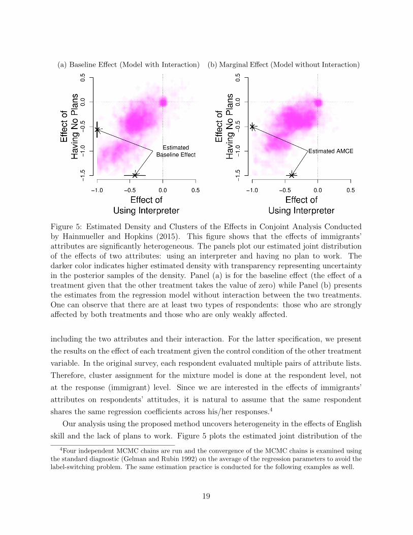
(a) Baseline Effect (Model with Interaction) (b) Marginal Effect (Model without Interaction)

Figure 5: Estimated Density and Clusters of the Effects in Conjoint Analysis Conductedby Hainmueller and Hopkins (2015). This figure shows that the effects of immigrants’attributes are significantly heterogeneous. The panels plot our estimated joint distributionof the effects of two attributes: using an interpreter and having no plan to work. Thedarker color indicates higher estimated density with transparency representing uncertaintyin the posterior samples of the density. Panel (a) is for the baseline effect (the effect of atreatment given that the other treatment takes the value of zero) while Panel (b) presentsthe estimates from the regression model without interaction between the two treatments.One can observe that there are at least two types of respondents: those who are stronglyaffected by both treatments and those who are only weakly affected.

including the two attributes and their interaction. For the latter specification, we present

the results on the effect of each treatment given the control condition of the other treatment

variable. In the original survey, each respondent evaluated multiple pairs of attribute lists.

Therefore, cluster assignment for the mixture model is done at the respondent level, not

at the response (immigrant) level. Since we are interested in the effects of immigrants’

attributes on respondents’ attitudes, it is natural to assume that the same respondent

shares the same regression coefficients across his/her responses.4

Our analysis using the proposed method uncovers heterogeneity in the effects of English

skill and the lack of plans to work. Figure 5 plots the estimated joint distribution of the

4Four independent MCMC chains are run and the convergence of the MCMC chains is examined usingthe standard diagnostic (Gelman and Rubin 1992) on the average of the regression parameters to avoid thelabel-switching problem. The same estimation practice is conducted for the following examples as well.

19

(a) Baseline Effect (Model with Interaction)

(b) Marginal Effect (Model without Interaction)

Figure 6: Heterogeneity within Subgroups by the Level of Ethnocentrism. This figureshows that the treatment effects are heterogeneous not across but within subsamples basedon the level of ethnocentrism. The panels plot our estimated joint distribution of theeffects of two attributes: using an interpreter and having no plan to work. The darkercolor indicates higher estimated density with transparency representing uncertainty in theposterior samples of the density. Panel (a) is for the baseline effect (the effect of a treatmentgiven that the other treatment takes the value of zero) while Panel (b) presents the estimatesfrom the regression model without interaction between the two treatments. One can observeheterogeneity in each plot, but the results from the same specification are similar acrosshigh/low levels of ethnocentrism.

20

two attributes, where the darker color represents higher estimated density. Results shown

in the figure present a pattern common across both regression specifications. On the one

hand, the estimated distribution indicates that the effects are in the same direction as the

original study for most respondents. On the other hand, the size of the effects varies across

respondents. There is a region with high densities at the bottom left in each plot, while

another region is found closer to the origin. These plots indicate that the effect of using

an interpreter and the effect of having no plans to work are correlated and heterogeneous.

There are some people who are strongly affected by both, whereas other people are only

weakly affected.

Figure 6 illustrates how the proposed method is useful in discovering treatment het-

erogeneity that is not predicted by observed variables. This figure is the same as Figure 5

except that the results for each of the subgroups the original study analyzed are shown

separately. In both rows, the left (right) panel is the results for the high (low) level of

ethnocentrism. The top row shows the results for the model including the interaction of

the two attributes, while the bottom row presents the results for the model without the in-

teraction term. All plots show significant heterogeneity in the treatment effects. However,

the plots look quite similar within each row. These results suggest that although there

is a consensus across subgroups with high and low ethnocentrism, there may well be an

unobserved cleavage in the American public. The treatment heterogeneity is not the con-

sequence of moderation by the level of ethnocentrism, and therefore it is hard to discover

it if researchers do not have a means to explore causal heterogeneity without relying on

observed variables.

4.2 Heterogeneity by an Omitted Variable: Effects of Indiscrim-

inate Violence

The second example illustrates how researchers can use the proposed Dirichlet mixture

model to uncover a moderator that is omitted from their specification. We reanalyze a

data set from a study on the effect of indiscriminate counterinsurgency violence (Lyall

2009), and discover heterogeneity in the treatment effect that the original study did not

find. In particular, our reanalysis reveals that the controversial conclusion of the original

study is limited to a particular period of the war. This example shows the utility of

the proposed method in a search for heterogeneous treatment effects when a researcher

overlooks an important moderator in hypothesizing what moderates the treatment effect.

The conventional wisdom in the literature on insurgency warfare is that indiscriminate

21

counterinsurgency violence is counterproductive. If the government kills or harms civilians

without making efforts to distinguish them from insurgents, it loses support from the local

population and guerrillas become more active. Such indiscriminate use of force causes

grievance among those who suffer it and motivates them to assist the guerrillas. Instead,

counterinsurgency operations must be selective. The government should choose targets

carefully and neutralize only combatants, so that it attracts the “hearts and minds” of the

non-combatants to suppress insurgency.

Lyall (2009) exploited a natural experiment to verify this claim. During the second

Chechen War, Russian military and security forces conducted a large scale counterinsur-

gency campaign in Chechnya. Observing the campaign, Lyall found that the Russian

artillery forces deployed to Chechnya randomly chose their targets. In fact, Russian mili-

tary doctrine recommends random shelling. The purpose of the artillery bases in Chechnya

was to complicate insurgent strategy using barrage patterns called “harassment and in-

terdiction,” which “is explicitly designed to consist of barrages at random intervals and

of varying duration on random days without evidence of enemy movement” (Lyall 2009,

p. 343). Moreover, recorded prosecutions of soldiers and eyewitness testimony suggest that

Russian soldiers fired field guns while inebriated. Their artillery attacks were clearly in-

discriminate because field artillery does not use precision-guided munitions. The shells

might not have just created craters in the ground; they may also have killed a number of

villagers and destroyed their houses. Also, these attacks dispersed unexploded ordnance,

making farms, lands, and forests unavailable. Although the situation is dire, it is a very

useful natural experiment to study the effect of indiscriminate violence. Lyall utilized this

randomness in the selection of the targets and examined the effect of the shellings on the

number of insurgent attacks against Russians.

Lyall’s results provide powerful counter-evidence against the conventional wisdom that

indiscriminate violence suppresses insurgency. His analysis showed that the Russian ar-

tillery bombings in fact reduced the number of guerrilla attacks. The data analysis was

thoroughly conducted and the results passed a number of robustness tests. He first created

353 matched pairs (therefore, N = 706) of a shelled (treated) village and a non-shelled

(control) village based on covariates such as population, altitude, a measure of poverty, the

religious brotherhood of villagers, whether a Russian garrison was stationed there, whether

a village was located in an area controlled by rebels, the number of sweep operations con-

ducted by ground troops in a village, and how isolated the village is. Then, he conducted a

difference-in-difference (DiD) analysis where the difference in the number of rebel attacks

22

before and after a shelling was the outcome variable. The DiD analysis with and without

regression adjustment for the covariates gave almost identical results and the estimated

average effect of Russian attacks was consistently negative.

As Lyall (2009, p. 357) notes, this conclusion is highly controversial—not only because

his evidence is the polar opposite to the conventional wisdom, but also because it suggests

a horrifying policy implication. If random use of force is actually effective in suppressing

insurgent violence, should governments facing insurgency indiscriminately attack local pop-

ulations, including non-combatants? Of course, Lyall emphasizes that his evidence should

not be interpreted as an endorsement of such a strategy. Attacking non-combatants is a

serious war crime, and he notes that his results only capture the short-term effects. On the

other hand, he admits that there may well be a suppressive effect of indiscriminate violence

at least in the short or medium term, and that this fact may explain why some militaries

adopt this strategy and commit war crimes (Lyall 2009, p. 357).

In light of this controversial evidence, it is of critical importance to examine treatment

heterogeneity. The conditions, if any, under which indiscriminate violence is effective in

suppressing insurgency would determine how much the conventional wisdom is questioned

and how broadly the policy implication applies. If, for example, the suppressive effect of

the Russian artillery attacks is observed only when a particular battlefield tactic is adopted

by the Russian military, then Lyall’s results may have to be interpreted as evidence that

the suppressive effect of random shellings is rather limited, even in the short-to-medium

term. Since adopting the suggested policy implication may be extremely harmful, the exact

conditions for indiscriminate violence to be effective must be thoroughly understood.

The proposed method discovers that the effect of artillery attacks is significantly hetero-

geneous. Here, we estimate the Dirichlet mixture regression model including the covariates

that the original study used to construct matched pairs. As in the original study, the out-

come variable is the difference in the number of rebel attacks before and after a shelling.

This is exactly the same as the analysis reported in Column 2 of Table 3 in Lyall (2009,

p. 350). The left panel of Figure 7 presents the estimated density of the treatment effect.

One can clearly see significant heterogeneity in the effect of random artillery attacks on

the number of insurgent attacks in the plot. While the estimated average effect (shown as

a cross mark in the figure) is negative and statistically significant, the estimated density is

bimodal, with a large spike at zero and another local mode at a negative value. The density

has a thicker tail on the negative values, so that the estimated average effect is negative.

The left panel of Figure 11 shows results from the estimation of the Dirichlet mixture re-

23

EstimatedATE

−2.0 −1.5 −1.0 −0.5 0.0 0.5

01

23

4

Effect Size

Den

sity

of E

stim

ated

Effe

cts

(a) Estimated Density of Causal Effect (b) Density Estimates by Attack Date

Figure 7: Estimated Density of the Effect of Artillery Attacks and Heterogeneous Effectsover Time (Estimated with Covariates). (1) The left panel shows that the effect of artillerybombings is significantly heterogeneous. A spike of the estimated density (x-axis) exists atzero effects (y-axis), while there is another local mode of the density near the estimatedaverage effect found by the original study. (2) The right panel indicates the source ofheterogeneity shown in the left panel. Each vertical line shows the density estimate ofthe effect (y-axis) for each date of attack (x-axis) where the darker color represents higherdensity. After December 2002, the density on negative values becomes higher.

gression model without any covariates as a robustness test, and the results are similar to

Figure 7 except that the estimation is less precise due to the lack of the covariates. These

results indicate that the negative effect of indiscriminate artillery attacks estimated in the

original study is driven by a subset of data, and that for a large proportion of Chechen

villages the random bombings did not have any suppressive effect.

Where does this heterogeneity come from? The right panel of Figure 7 provides an

answer to the question. The estimated density of the effect is shown for each date of attack

(the x-axis) in this plot, and the darker color represents the region of the effect size that has

higher density for a particular day. That is, each vertical line is the density seen from the

top with the color representing values of the density. The plot clearly shows that the effect

of indiscriminate violence is observed only after late 2002. Until late 2002, the estimated

effect is consistently close to zero, while large negative effects are estimated after that.

The same conclusion is obtained from the right panel of Figure 11, although the estimated

effect becomes negative a little later than the main results. These results show that the

conclusion of Lyall’s original study is driven by the artillery attacks after late 2002 (or early

2003).

24

Given the available data, we can only conjecture as to the reason for the aforementioned

heterogeneity. However, the pattern we find is consistent with an observed change of Rus-

sia’s counterinsurgency strategy. In 2002, Russians started experimenting joint counterin-

surgency patrols with Chechen police, which was followed by the formation of Chechen-only

patrol units in early 2003. As a result of this “Chechenization” of the conflict, sweep op-

erations by ground troops were conducted more often by units consisting of pro-Russian

Chechens in and after 2002 (Lyall 2010). The empirical results discussed above seem to

suggest that the repressive effect of indiscriminate artillery attacks existed only when sweep

operations were conducted by co-ethnic troops. Further exploration of whether this strate-

gic change is in fact the source of the heterogeneity is beyond the scope of this paper.

4.3 Densities within Subgroups: Effects of Voter Audits

In the third example, we illustrate the utility of the proposed Dirichlet process mixture

model for another purpose. Using a study on the effect of voter audits on the inflow of

registered voters (Hidalgo and Nichter 2015), we show that the proposed method allows

researchers to examine treatment heterogeneity across predefined subgroups in more detail

than simply estimating the average effects within the subgroups. Specifically, while the

original study claims that the average effect of voter audits varies across two subgroups

split at the median value of a covariate, our reanalysis using the proposed method shows

that the difference between the estimated densities of the effect for the two subgroups

results from the tails of the densities. This example illustrates how researchers can use the

proposed method to improve their inference on causal heterogeneity when they have some

prior expectation regarding how heterogeneous the effect is.

Hidalgo and Nichter (2015) tried to show evidence for a less discernible means of election

fraud, voter buying. Voter buying is an indirect practice in the sense that it is not an

attempt to influence the actions of the electorate. In contrast to more direct fraud such

as vote buying, voter buying is an endeavor to shape the composition of the electorate by

bringing favorable voters in. Especially in local elections, where some regions in a country

conduct elections but others do not, politicians may well try to pull outsiders into their

district expecting that those outsiders will vote for them. If the terms of local offices are

fixed so that the electoral cycles are highly predictable, voter buying is easier because

politicians know when exactly they need voters in their district.

Brazil provides an excellent environment to find evidence for voter buying. Municipal

mayors and councilors have fixed terms and are elected concurrently every four years, while

25

federal elections occur two years after every municipal election. That is, local politicians

clearly realize that they want to “buy voters” every four years in order to win their elec-

tions. In fact, Hidalgo and Nichter (2015) show that the number of registered voters in

municipalities surrounding state capitals increases in the year of every municipal election

and decreases in the year of every federal election. The opposite pattern is observed for

the number of registered voters in state capitals, which suggests that municipal politicians

in rural areas are importing voters from cities in the year of their elections.

The core part of empirical analysis by Hidalgo and Nichter (2015) is exploiting the in-

stitutional threshold that triggers voter audits. In Brazil, a municipality becomes eligible

for voter audits when its electorate size exceeds 80% of the total population. Although the

threshold does not completely determine the assignment of voter audits (some municipali-

ties below the threshold get audits and some above do not), one can exploit the variation

caused by the threshold using a fuzzy regression discontinuity (FRD) design. In this con-

text, we would like to know the effect of voter audits on the registered voter inflows because

the negative effect of audits strongly suggests the existence of voter buying. The fact that

the voter audits reduce voter inflows should imply that some inflows are prevented due

to being audited (i.e. the prevented portion of inflows would have been fraudulent voter

buying if the voter audits had not been conducted). Employing the FRD design, the au-

thors of the original study found a large negative effect of voter audits on the inflows of

registered voters. In fact, the estimated effect suggests that receiving a voter audit reduces

the change in the number of registered voters by 12% of the total population.

Hidalgo and Nichter (2015) further explored evidence of voter buying. They hypothe-

sized that the effect of voter audits should be larger when more voters were imported in

previous years because the fact that many voters were imported into a municipality was

suggestive evidence for the existence of voter buying in it. The authors split the data set

into two groups, namely municipalities with previous voter inflows below and above the

median. They obtained the FRD estimate for each group and found that the results were

consistent with their hypothesis. Voter audits have a larger negative effect in municipalities

with previous voter inflows greater than the median.

We reconsider this treatment heterogeneity found in the original study. Since the FRD

design is equivalent to an IV analysis, we use the Dirichlet process mixture simultaneous

equations model developed in Section 2. Except for having the Dirichlet process mixture,

our analysis exactly follows Hidalgo and Nichter (2015). The analysis relies on a data set

from the 2007-08 wave of voter audits, whose assignment uses the ratio of the electorate to

26

EstimatedLATE

−30 −20 −10 0 10 200.

000.

020.

040.

060.

080.

10

Effect Size

Den

sity

of E

stim

ated

Effe

cts

(a) Estimated Density of Treatment Effects

(b) Estimated Density and Previous Inflow (c) QQ Plot for Subgroups

Figure 8: Estimated Density of the Effect of Voter Audit and Heterogeneity across Sub-groups. Two panels of this figure show that the effect of voter audits on voter inflowsis rather homogeneous. (a) The top panel presents the estimated density of the effect ofaudits with the estimated local average treatment effect in the original study. The esti-mated density is unimodal and does not show any significant heterogeneity of the effect.(b) The bottom left panel plots the estimated density of the treatment effect for each ob-served value of previous voter inflows. Gray vertical lines are drawn for observed values ofprevious voter inflows and ranges with darker magenta represent effect sizes with higherdensities. (c) The bottom right panel displays the QQ plot of the estimated densities forthe two subgroups defined by Hidalgo and Nichter (2015). The x-axis is for the subgroupwith previous inflows above the median, while the y-axis is for the subgroup with previousinflows below the median. The plot shows that the two densities are quite similar in thelocation of the mass of the densities. The difference is observed only in the tails, whichsuggests that focusing on the average effects overlooks why the two groups are different.

27

the population in 2007. The outcome variable is the change in the size of the electorate from

2007 to 2008 relative to the population in a municipality. The instrument is whether the

electorate size exceeded the threshold (80% of the population) in 2007 and the treatment

is whether a municipality received audits. We fit the model with a bandwidth of ±1.5%

yielding 577 municipalities in the data and include the forcing variable (the proportion of

the electorate in the total population) in the model as a pretreatment covariate.

Our results are summarized in Figure 8. First, Panel 8a shows that the estimated density

of the effect of voter audits is largely homogeneous. It presents the estimated density with

the local average treatment effect estimated by the original study (a cross mark in the

plot). Contrary to the previous example, the density is unimodal and concentrated around

the estimated average effect. Although the right tail of the density is thicker than the other

tail, no significant heterogeneity is observed in this plot.

The bottom two panels of Figure 8 reexamine the heterogeneity that Hidalgo and

Nichter (2015) found. In fact, the panels indicate that the estimated densities of the

effect are quite similar across the two subgroups the original study focused on. Panel 8b

presents the estimated density of the treatment effect for each observed value of previous

voter inflows. It shows that there is one value of previous voter inflows, which is right below

2, 000, such that high density regions are located at large negative values. However, any

significant heterogeneity does not exist for the other observed values of previous inflows.

Panel 8c displays the QQ plot for the two subgroups defined in the original study. The

first subgroup contains the municipalities with the number of voter inflows from 2005-2006

greater than the median (180), while the second subgroup consists of the other munici-

palities. The estimated quantiles of the effect of audits for the first group are shown in

the x-axis, while those for the second group are shown in the y-axis. As one can readily

see, the two densities are almost identical in the location of the mass of the densities. For

the effect size from −50 to 50 the plotted quantiles are very close to the 45-degree line,

which indicates that the two distributions have the same shape for the values in this in-

terval. Although a difference between the two densities is observed in the tails and this

difference seems to be the source of heterogeneity in the average effects across subgroups,

our conclusion is that heterogeneity is largely nonexistent across these subgroups.

4.4 Changing Subgroups: Effects of Natural Disaster

The last example illustrates how the proposed method can be used in the context of IV

analysis. We show that the method can assess the validity of the monotonicity assumption

28

and improve subgroup analysis often conducted by applied researchers to address possi-

ble violation of the assumption. Reanalysis of a data set from a study on resource curse

(Ramsay 2011) shows that researchers can employ the proposed method to uncover het-

erogeneity in the effect of an instrumental variable on a treatment. In particular, we focus

on the original study’s claim about the first-stage negative effect of natural disasters on oil

revenues and challenge this assumption. While the original study checks the robustness of

the claim by running regressions on multiple subgroups, we argue that the membership of

those heterogeneous subgroups may well change over time. Using the proposed method,

researchers can find how countries consisting of the subgroups change over time.

The resource curse is one of the most well known hypotheses in comparative politics.

It claims that having a rich supply of natural resources (e.g., oil) prevents a country from

democratizing. Although the hypothesis is widely known, empirical controversy remains

(e.g. Haber and Menaldo 2011; Andersen and Ross 2013). To empirically prove or deny the

resource curse hypothesis is difficult because reliance on natural resources and the type of

political regime may have reverse causality, and because many unobserved confounders are

expected to exist.

Ramsay (2011) addresses this difficulty by employing an IV analysis. Ramsay uses

the occurrence of natural disasters, in particular “out of region disaster damage for oil-

producing nations.” He claims that natural disasters in other regions of the world do not

directly affect the political regime of an oil-producing country, but that they do affect its

oil revenues through the effect on world oil prices. For example, Hurricane Katrina in the

United States (US) would not directly affect Saudi Arabia’s political regime. However, the

storm would affect Saudi Arabia’s oil revenues because it destroyed at least 113 off-shore

platforms and therefore raised the price of oil. To satisfy the exclusion restriction, Ramsay

constructed his instrumental variable as follows. First, he focused on five types of natural

disasters that were relevant to world oil prices but would not be considered to have an

impact on the political regime of a distant nation.5 Second, to instrument the oil revenues

of an oil-producing country, he used natural disasters that happened in another region of

the world. To be precise, he divided the world into five regions and only used disasters

that occurred in a different region from the one to which the country belongs.6 Since the

occurrence of natural disasters is exogenous, the lack of direct effect of natural disasters on

political regimes guarantees the validity of disaster damage as an instrumental variable.

5The five categories are earthquakes, volcanos, mudslides, waves and surges, and windstorms.6The five regions are Europe, the Middle East and North Africa, sub-Saharan Africa, Asia, and the

Americas.

29

Figure 9: Estimated Posterior Mean of the Effect of Natural Disasters on Oil Revenuesfor Each Country. This map clearly shows that the assumptions made in the IV analysisare violated. For the countries shown in orange the estimated posterior mean of the firststage effect is positive, while the estimated posterior mean is negative for the countriesshown in blue. With a few exceptions, developed oil producers are negatively affected byout-of-region natural disasters and developing producers are positively affected.

We focus on the first stage effect in our reanalysis of Ramsay’s data set. That is, we

explore heterogeneity in the effect of out-of-region natural disaster damage on oil revenues.

Examining the heterogeneity of the first stage effect is particularly important because its

monotonicity is assumed to identify a treatment effect (Angrist, Imbens, and Rubin 1996).

If we observe that the effect of disasters is positive for some countries and negative for the

others, the assumption of the IV analysis is violated.

To empirically verify the assumption for the IV analysis, we fit the proposed Dirichlet

mixture IV model presented in Section 2 and examine our estimate of the effect for each

observation. As in the previous examples, we followed the original study (Ramsay 2011)

in virtually all aspects of data analysis. The data set includes the 48 countries that had

non-negligible oil production reported by British Petroleum from 1968-2002. Since it is an

unbalanced panel data set, it contains 1277 observations in total. The outcome is the regime

type measured by POLITY IV scores, the treatment is logged per capita oil income,7 and

the instrument is the out-of-region disaster damage described above. We included logged

GDP per capita and GDP growth in the model as pretreatment covariates.

The results for the first stage effect of natural disaster on oil revenues are shown in

Figure 9. The most important observation is that the estimation assumptions of the IV

7Calculated as “the product of the average daily spot price of crude oil [...] and a country’s annualproduction for that year (in barrels) divided by the population” (Ramsay 2011, p. 510).

30

(a) 1968 (b) 2002

Figure 10: Changing Subgroup Membership over Time: Estimated Posterior Mean, 1968and 2002. The two maps displayed in this figure show how the subgroup membershipchanged over time. As in Figure 9, for the countries shown in orange the estimated posteriormean of the first stage effect is positive while the estimated posterior mean is negative forthe countries shown in blue. One can observe that Latin American countries and SoutheastAsian countries moved from one subgroup to the other between 1968 and 2002. Thosecountries’ oil revenues were increased by out-of-region natural disasters in 1968, while in2002 the countries were affected by disasters in the same manner as the developed oilproducers such as the United States and Australia.

analysis are not supported. The map displays the estimated posterior mean of the effect of

out-of-region disaster damage on oil revenues for each country by colors where orange (blue)

represents a positive (negative) effect.8 For example, oil revenues for countries in the Middle

East (Saudi Arabia, Iran, and Iraq) rise when a natural disaster happens in other regions.

In fact, this is the direction of the first stage effect both expected and estimated by Ramsay

(2011). However, according to our point estimates, the US, Canada, and Australia’s oil

revenues decrease when a disaster occurs in the other regions. In other words, the first

stage effect is not monotonic, let alone homogeneous. Therefore, our analysis does not

support the estimation assumptions for the IV analysis.

Ramsay conducted robustness tests by running IV analyses on several subsets of the

data. He analyzed four subpopulations—the non-Western countries, the countries that

have state oil companies, the countries without top oil producers, and former colonies. In

all analyses, the main result holds true.

Our proposed method can provide a better insight than robustness analyses on several

different subsets of the data. Specifically, it is able to detect the changing membership of

subgroups over time. Figure 10 demonstrates this ability of the method. The left panel

shows the estimated first stage effect in 1968 (the beginning of the data set), whereas

the right panel displays the same quantity for 2002 (the last year in the data). One can

see a clear pattern in the shift of the subgroup structure. Countries in Latin America

8Figure 12 in the appendix presents the 90% and 95 % credible intervals for each country.

31

(e.g., Brazil, Argentina, and Mexico) and in Southeast Asia (e.g., Indonesia and Malaysia)

switched from the subgroup with the positive effect of disasters to the subgroup with the

negative effect. This example indicates a clear advantage of the proposed method over

approaches with predetermined subgroups, because the latter cannot help understand how

the countries comprising subgroups change over time.

5 Conclusion

In virtually all causal relationships treatment effects are thought to be heterogeneous. The

approach shared by existing methods for estimating heterogeneous treatment effects is to

find the subsamples across which the effect of a treatment differs. An issue with this

common approach is that researchers are required to know and observe the variables that

moderate the treatment effect. In many cases, researchers do not know what the moderators

are, and even when they do, some of the moderators are unobserved or mismeasured.

To address this issue, this paper proposed a Bayesian nonparametric approach that

estimates heterogeneity in causal effects without relying on observed variables hypothesized

as moderators. The proposed approach employs a Dirichlet process mixture model, where

each mixture component is associated with a distinct causal parameter and the number

of the components is estimated. Regularization from the Dirichlet process prior allows

researchers to consistently estimate the density of the unit-specific causal parameters, so

that causal heterogeneity is nonparametrically estimated.

The value of the proposed method was illustrated by four empirical applications. First,

the method can be used to discover treatment heterogeneity driven by unknown mod-

erators. We applied the proposed method to the data used by a study on Americans’

attitudes toward immigrants and showed that the proposed method discovered treatment

effect heterogeneity unexplained by the observed variables that the literature expected to

moderate the effect. Second, the method finds omitted moderators due to misspecification.

We reanalyzed the data used by a study on the effect of indiscriminate counterinsurgency

violence on the number of attacks initiated by insurgents in Chechnya and found that there

was significant heterogeneity attributable to time. Third, researchers can use the proposed

method to explore how a prespecified moderator changes treatment effects. We applied

the method to a study on the effect of voter audits on election fraud in municipalities of

Brazil using a fuzzy regression discontinuity (RD) design. We found that the heterogeneity

found by the original study stems from the tails of the distribution of treatment effects.

32

Finally, the proposed method can be used to diagnose the monotonicity assumption re-

quired for instrumental variable analysis that the effect of the instrument on the treatment

is in the same direction for all units. A study on the resource curse using natural disas-

ter as an instrument for oil revenues was reanalyzed and it is found that the direction of

the instrument’s effect is likely to differ across countries, which violates the monotonicity

assumption.

33

References

Andersen, Jørgen J, and Michael L Ross. 2013. “The Big Oil Change A Closer Look at theHaber–Menaldo Analysis.” Comparative Political Studies 47 (7): 993–1021.

Angrist, Joshua D., Guido W. Imbens, and Donald B. Rubin. 1996. “Identification of CausalEffects Using Instrumental Variables.” Journal of the American Statistical Association91 (June): 444–455.

Antoniak, Charles E. 1974. “Mixtures of Dirichlet Processes with Applications to BayesianNonparametric Problems.” The Annals of Statistics 2 (6): 1152–1174.

Athey, Susan, and Guido W Imbens. 2015. “Machine Learning Methods for EstimatingHeterogeneous Causal Effects.” Working Paper.

Caner, Mehmet. 2009. “Lasso-Type GMM Estimator.” Econometric Theory 25 (01): 270–290.

Chib, Siddhartha, and Barton H Hamilton. 2002. “Semiparametric Bayes Analysis ofLongitudinal Data Treatment Models.” Journal of Econometrics 110 (1): 67–89.

Conley, Timothy G, Christian B Hansen, Robert E McCulloch, and Peter E Rossi. 2008.“A Semi-Parametric Bayesian Approach to the Instrumental Variable Problem.” Journalof Econometrics 144 (1): 276–305.

Ding, Peng, Avi Feller, and Luke Miratrix. 2015. “Randomization Inference for Treat-ment Effect Variation.” Journal of the Royal Statistical Society: Series B (StatisticalMethodology).

Ding, Peng, Avi Feller, and Luke Miratrix. 2016. “Decomposing Treatment Effect Varia-tion.” arXiv preprint arXiv:1605.06566.

Escobar, Michael D, and Mike West. 1995. “Bayesian Density Estimation and InferenceUsing Mixtures.” Journal of the american statistical association 90 (430): 577–588.

Ferguson, Thomas S. 1973. “A Bayesian Analysis of Some Nonparametric Problems.” TheAnnals of Statistics 1 (2): 209–230.

Foster, Jared C, Jeremy MG Taylor, and Stephen J Ruberg. 2011. “Subgroup Identificationfrom Randomized Clinical Trial Data.” Statistics in Medicine 30 (24): 2867–2880.

Gautier, Eric, and Alexandre Tsybakov. 2011. “High-Dimensional Instrumental VariablesRegression and Confidence Sets.” arXiv preprint arXiv:1105.2454.

Gelman, Andrew, and Donald B Rubin. 1992. “Inference from Iterative Simulation UsingMultiple Sequences.” Statistical Science 7 (4): 457–472.

34

Ghosal, Subhashis, Jayanta K Ghosh, RV Ramamoorthi et al. 1999. “Posterior Consistencyof Dirichlet Mixtures in Density Estimation.” The Annals of Statistics 27 (1): 143–158.

Gill, Jeff, and George Casella. 2009. “Nonparametric Priors for Ordinal Bayesian SocialScience Models: Specification and Estimation.” Journal of the American Statistical As-sociation 104 (486): 453–454.

Green, Donald P, and Holger L Kern. 2012. “Modeling Heterogeneous Treatment Effects inSurvey Experiments with Bayesian Additive Regression Trees.” Public Opinion Quarterly76 (3): 491–511.

Grimmer, Justin, Solomon Messing, and Sean J Westwood. 2016. “Estimating Heteroge-neous Treatment Effects and the Effects of Heterogeneous Treatments with EnsembleMethods.” Working Paper.

Haber, Stephen, and Victor Menaldo. 2011. “Do natural resources fuel authoritarianism?A reappraisal of the resource curse.” American Political Science Review 105 (1): 1–26.

Hainmueller, Jens, and Daniel J Hopkins. 2015. “The Hidden American Immigration Con-sensus: A Conjoint Analysis of Attitudes toward Immigrants.” American Journal ofPolitical Science 59 (3): 529–548.

Hainmueller, Jens, Daniel J Hopkins, and Teppei Yamamoto. 2014. “Causal Inferencein Conjoint Analysis: Understanding Multidimensional Choices via Stated PreferenceExperiments.” Political Analysis 22 (1): 1–30.

Hannah, Lauren A, David M Blei, and Warren B Powell. 2011. “Dirichlet Process Mixturesof Generalized Linear Models.” Journal of Machine Learning Research 12 (Jun): 1923–1953.

Hidalgo, F Daniel, and Simeon Nichter. 2015. “Voter Buying: Shaping the Electoratethrough Clientelism.” American Journal of Political Science 60 (2): 436–455.

Imai, Kosuke, and Aaron Strauss. 2011. “Estimation of Heterogeneous Treatment Effectsfrom Randomized Experiments, with Application to the Optimal Planning of the Get-Out-the-Vote Campaign.” Political Analysis 19 (1): 1–19.

Imai, Kosuke, and Marc Ratkovic. 2013. “Estimating Treatment Effect Heterogeneity inRandomized Program Evaluation.” The Annals of Applied Statistics 7 (1): 443–470.

Imbens, Guido W, and Donald B Rubin. 2015. Causal Inference in Statistics, Social, andBiomedical Sciences. Cambridge University Press.

Ishwaran, Hemant, and Lancelot F James. 2001. “Gibbs Sampling Methods for Stick-Breaking Priors.” Journal of the American Statistical Association 96 (453).

35

Kyung, Minjung, Jeff Gill, and George Casella. 2011. “New Findings from TerrorismData: Dirichlet Process Random-Effects Models for Latent Groups.” Journal of the RoyalStatistical Society: Series C (Applied Statistics) 60 (5): 701–721.

Kyung, Minjung, Jeff Gill, George Casella et al. 2010. “Estimation in Dirichlet RandomEffects Models.” The Annals of Statistics 38 (2): 979–1009.

Lyall, Jason. 2009. “Does Indiscriminate Violence Incite Insurgent Attacks? Evidence fromChechnya.” Journal of Conflict Resolution 53 (June): 331–362.

Lyall, Jason. 2010. “Are coethnics more effective counterinsurgents? Evidence from thesecond Chechen war.” American Political Science Review 104 (01): 1–20.

Neal, Radford M. 1992. “Bayesian Mixture Modeling.” In Maximum Entropy and BayesianMethods. Springer.

Ramsay, Kristopher W. 2011. “Revisiting the Resource Curse: Natural Disasters, the Priceof Oil, and Democracy.” International Organization 65 (03): 507–529.

Rasmussen, Carl Edward. 1999. “The Infinite Gaussian Mixture Model.” In NIPS. Vol. 12Vol. 12.

Ratkovic, Marc, and Dustin Tingley. 2015. Sparse Estimation and Uncertainty with Appli-cation to Subgroup Analysis. Technical report Working Paper available a t https://www.princeton. edu/˜ ratkovic/public/sparsereg. pdf.

Rubin, Donald B. 1974. “Estimating Causal Effects of Treatments in Randomized andNonrandomized Studies.” Journal of Educational Psychology 66 (5): 688.

Sethuraman, Jayaram. 1994. “A Constructive Definition of Dirichlet Priors.” Statisticasinica 4 (2): 639–650.

Shahn, Zach, and David Madigan. 2016. “Latent Class Mixture Models of Treatment EffectHeterogeneity.” Bayesian Analysis.

Su, Xiaogang, Chih-Ling Tsai, Hansheng Wang, David M Nickerson, and Bogong Li. 2009.“Subgroup Analysis via Recursive Partitioning.” Journal of Machine Learning Research10 (Feb): 141–158.

Teh, Yee Whye. 2010. “Dirichlet Process.” In Encyclopedia of Machine Learning. Springer.

Wiesenfarth, Manuel, Carlos Matıas Hisgen, Thomas Kneib, and Carmen Cadarso-Suarez.2014. “Bayesian Nonparametric Instrumental Variables Regression Based on PenalizedSplines and Dirichlet Process Mixtures.” Journal of Business & Economic Statistics32 (3): 468–482.

Zeileis, Achim, Torsten Hothorn, and Kurt Hornik. 2008. “Model-based Recursive Parti-tioning.” Journal of Computational and Graphical Statistics 17 (2): 492–514.

36

A Gibbs Sampler Algorithm for the Dirichlet Process

Mixture

Here, we describe the blocked Gibbs sampler algorithm with the truncation approximationwe use to estimate the Dirichlet process mixture model. First, we set a large number Kat which we truncate the number of mixture components. In practice, K = 25 or 50 iscommonly chosen as a default, but it can be arbitrarily large. In all of the example above,the results are insensitive to the choice of K = 40 and 100.

At the beginning of the algorithm, we set the starting values of k[i] for all i = 1, . . . , Nand τk′ and γk′ for all k = 1, . . . , K. For each k′, we define

Wk′ = [Tk′ Xk′ ]

where Tk′ and Xk′ is the matrix of treatments and covariates whose rows are observationswith k[i] = k′. We also define βk′ ≡ (τ>k′ , γ

>k′)> Then, each iteration of the Gibbs sampler

proceeds as follows:

1. Update σk′ for k′ = 1, . . . K by sampling from a scaled inverse χ2 distribution with

σ2k′ ∼ Scale-inv-χ2(ν +Nk′ ,

νs2 +Nk′ s2k′

ν +Nk′)

where Nk′ =∑N

i=1 1{k[i] = k′}, p is the number of treatments and pretreatmentcovariates, and

s2k′ ≡1

Nk′ − p(Yk′ −Wk′βk′)

>(Yk′ −Wk′βk′).

2. Update τk′ and γk′ for k′ for k′ = 1, . . . , K by sampling from a Gaussian distributionwith

βk′ ∼ N((∆0 +W>

k′Wk′)−1W>

k′Yk′ , (∆0 +W>k′Wk′)

−1σ2k′

)where

∆0 ≡[δτ 0>

0 ∆γ

].

3. Update the stick-breaking weight πk′ for k′ = 1, . . . , K − 1 by sampling from a Betadistribution with

πk′ ∼ Beta

(1 +Nk′ , α +

K∑l=k′+1

Nl

)

37

4. Update k[i] ∈ {1, . . . , K} for i = 1, . . . , N by multinomial sampling with

Pr(k[i] = k′) ∝ pk′N (sik′ | βk′ , σk′)

where

pk′ ≡ πk′k′−1∏l=1

(1− πl)

sik′ ≡ Yi − Tiτk′ −X>i γk′ .

38

B Additional Figures for Empirical Analysis

EstimatedATE

−3 −2 −1 0 1

01

23

4

Effect Size

Den

sity

of E

stim

ated

Effe

cts

(a) Estimated Density of Causal Effect (b) Density Estimates by Attack Date

Figure 11: Estimated Density of the Effect of Artillery Attacks and Heterogeneous Effectsover Time (Estimated without Covariates). As a robustness check for Figure 7, the Dirichletmixture regression model is estimated without covariates. (1) The left panel shows that theeffect of artillery bombings is significantly heterogeneous. A spike of the estimated density(x-axis) exists at zero effects (y-axis) while there is another local mode of the density nearthe estimated average effect by the original study. (2) The right panel indicates the sourceof heterogeneity shown in the left panel. The figure shows the density for the dates ofattacks (x-axis) and the effect size (y-axis) where darker color represents higher density.Starting in December 2002, negative effects get higher densities.

39

Effect Size

NorwayColombia

Trinidad & TobagoIndia

VenezuelaCanada

USAAustraliaDenmark

United KingdomEcuador

ItalyRussian Federation

YemenMalaysia

KazakhstanArgentinaThailand

BrazilAngolaNigeria

PeruAzerbaijan

MexicoRomania

EgyptIran

IndonesiaAlgeriaTunisia

CameroonRep. of Congo (Brazzaville)

TurkmenistanGabon

UzbekistanIraq

Saudi ArabiaSyria

KuwaitLibyaOman

United Arab EmiratesChina

VietnamSudan

−0.2 0.0 0.2 0.4 0.6

Figure 12: Estimated Posterior Mean and Credible Intervals of the Effect of Out-of-RegionNatural Disasters on Oil Revenues. This figure shows that the effect of the instrumentalvariable on the treatment in Ramsay (2011) is likely to be non-monotonic. The posteriormean for each country and the 90% and 95% credibility intervals are shown. For manycountries, the effect is positive and significant. On the other hand, for some countries pointestimates are negative and indistinguishable from zero. These results do not support theassumption of monotonic/homogeneous first-stage effects.

40