0  

United States Department of Agriculture Office of the Chief Economist Office of Energy Policy and New Uses Agricultural Economic Report Number 847 November 2012  

 

Biomass Supply From Corn Residues:   

Estimates and Critical Review of Procedures   

 

 

Paul W. Gallagher Department of Economics Iowa State University 

 Harry Baumes 

Director, Office of Energy Policy and New Uses Office of the Chief Economist, USDA   

   

    

1  

Table of Contents 

Introduction ……………………………………………………………………………………………………………….……..2 

Overview of Estimation and Calculation Procedures.………………………………………………….…….2 

Harvest Index………………………………………………………………………………..……………………..4 

Sustainability……………………………………………………………………………………................... .6 

Stover Feed Demand ……………………………………………………………………………………………9 

Stover Supply for Industry………………………………………………….…………………………….. 11 

Farm Cost…………………………………………………………………………..………..………………………………….13 

Farm Cost Estimates…………………………………………………………………………………………..13 

Handling Costs……………………………………………………………………………………………………15 

Handling Cost Estimates…………………………………………………………………………………….15 

Delivered Plant Cost ………………………………………………………………………………………….16 

U.S. Stover Supply Schedule…………………………………………………………………………………………..19 

Conclusions………………………………………………………………………………………………………..............19 

References ……………………………………………………………………………………………………………………..21 

Appendices 

A:  Stover Harvest and Soil Carbon Maintenance  ………………………………………………………… 23 

B:  County Estimates of Stover Availability and Cost….………………………………………............ 27 

C:  Estimates of Stover Harvest Season Length  ……………………………………………….……………..27 

The U.S. Department of Agriculture (USDA) prohibits discrimination in all its programs and activities on the basis of race, color, national origin, age, disability, and, where applicable, sex, marital status, familial status, parental status, religion, sexual orientation, genetic information, political beliefs, reprisal, or because all or a part of an individual's income is derived from any public assistance program. (Not all prohibited bases apply to all programs.) Persons with disabilities who require alternative means for communication of program information (Braille, large print, audiotape, etc.) should contact USDA's TARGET Center at (202) 720-2600 (voice and TDD). To file a complaint of discrimination write to USDA, Director, Office of Civil Rights, 1400 Independence Avenue, S.W., Washington, D.C. 20250-9410 or call (800) 795-3272 (voice) or (202) 720-6382 (TDD). USDA is an equal opportunity provider and employer.   

    

2  

Introduction

Some early estimates suggested that accessible and sustainable corn residue supplies are adequate for a new biomass processing industry (Gallagher and Johnson; Gallagher, et al 2003a; Gallagher, et al 2003b). Revision is justified now because the agronomic and economic environment has changed. There is also interest in the location of low cost supplies, because construction of biomass processing facilities is underway. A critical review for suitable cost estimation assumptions and sustainability concepts should also be incorporated in the revised estimates, given subsequent discussion.

The corn stover cost and supply estimates presented here fit today’s yield and input situation. The revised estimates confirm that corn stover supplies are still adequate for new processing activity; several offsetting changes in economic environment and technology combine for a total supply estimate that is slightly larger and cost estimates that are highly competitive in today’s energy markets. The location and extent of lowest cost and sustainable supplies are also given.

This paper is organized as follows. First, we summarize the supply model. Second, we present new data and spatial variation in critical parameters that impinge on estimates of usable supply: current estimates of the harvest index, local feed demand, and a conservation allowance are discussed in turn. We compare our assumptions with the literature, justifying, incorporating, and discarding as appropriate.

Overview of Estimation and Calculation Procedures

Stover output and cost are calculated for every corn-producing county in the United States, using a series of identities and proportional relationships that are defined by agronomy and current technology. Four groups of relations calculate production, feed demand, cost, and U.S. supply. The stover production group includes a relation that defines stover output as a proportion of the corn crop, and specifies the amount of stover that must remain on the field for soil conservation. The feed demand block calculates the excess demand defined by the forage demands of local livestock less hay and pasture supply. Potential industry supply to stover is production less feed demand. Costs include farm harvest (rake, bale fertilize) expenditure and handling costs such as shipping and storage. Lastly, county data is ordered by cost, and aggregated for a U.S.-level supply curve. The relationships are summarized in table 1.

This report includes revised data and critical evaluation of important assumptions. Revisions include current data for agronomic and economic relationships. Specifically, current estimates for county corn yields, harvest index estimates, cattle populations, and energy input prices are employed. Local estimates are calculated for a conservation allowance of residue remaining after harvest and a sustainable fraction of corn area that is suitable for residue harvest while maintaining soil quality.

    

3  

Table 1. County and U.S. Corn Stover Supply Model

Variable Definitions

(1) Stover Production:

 Ysg = [ (1‐hi)/hi ] Yc θ 

Ysn = Ysg – Ca

As= Ac * sf * fr

Qsp = Ysn * As

(2)Stover Feed Demand:

Nfd = (Fdb+Fdm) – (Qpp + Qpwp + Qhp )

Fdb = 27.6 Cob+13.2Hb+30 Bu+5.8 Ho+8.8 Ca 

Fdm=25.2Com + 9.6Hm 

Qpp = dg * Fdb 

Qwp=135 * Fdb 

(3)Cost:

Cst =β f + αf / Ysn

Cstd = Cst + βT +  βs

 (4)Supply: 

(a)Stover Supply to Industry: Nssi = Qsp – Nfd

      (b)Supply Function:                                                                                                                                                   

‐Develop short list of counties (839 of 2805) from the condition that Cstd < $100/ton, and the 

requirement that 20 surrounding counties or less would be required for a 25 MGY ethanol plant. ‐

Sort on Cstd and cumulate Nssi. 

 

   

Yc: yield , corn  ;  hi: harvest index;                                                                                      

Parameters    θ : adjustment for no till yield discount( and unit conversions)  

Ysg: Yield stover,gross;  Ysn: Yield stover, net(in ton/acre);                             

Ca: Conservation allowance;                                                                                  

As: Area, sustainable(fraction of corn area); Ac: Area, corn (in mil acre);     

sf: sustainable fraction( of corn area);  fr: fraction in rotation                         

Qsp: Quantity of Stover produced (in mil ton);                                           

Nfd: Net feed demand(for stover); Fdb:Feed demand , beef; Fdm: Feed 

demand, milk; Qpp: Quantity pasture ; Qpwp: Quantity, winter wheat pasture; 

Qhp: Quantity of hay produced  

Cob: cows, beef;   Hb: heifer, beef;   Bu: bull; Ca:calves;   Com: cows,milk;   Hm: 

heifer, milk;  

Parameters:  dg: degree‐days(growing season);             135: length of wheat 

pasture season                          

Nssi: Net Supply to Industry 

Cst: Cost of stover, farm (in $/ton) 

Paramaters: α acre constant costs (cut,rake bale); 

 β ton constant costs(field haul) 

Cstd:  Cost of Stover, delivered to plant 

Parameters:  βT: transport costs to plant,   βs:Storage Costs 

    

4  

Harvest Index 

The harvest index is defined at corn grain’s proportion of the total above ground dry biomass in the corn plant:

hi= dry weight grain / ( dry weight grain + dry weight residue) on an acre

Previously, the harvest index was taken as a constant, hi=0.45, based on measurements from an Iowa experiment. Thus, the fraction of stover in the biomass, 1-hi=0.55. That is, stover provided 55 percent of the total biomass in corn.

Subsequently, corn yields have typically increased and the harvest index has declined. Our revised estimates are based on a recent report from a Pioneer/Monsanto project with very recent yield levels and varieties (Edgerton). hi is generally lower, possibly because corn yield increases of the last decade were accomplished with higher plant populations. Specifically, we assume that there is a cubic relation between corn yield and harvest index:

hi = ϒ0 + ϒ1 Yc1 + ϒ2 Yc2+ ϒ3 Yc3 , where ϒi are parameters for estimation.

An estimate based on the 2008 cross section of plots yields from the Monsanto Experiment is given in figure 1. In supply estimation at the county level, county corn yield data are used in the cubic harvest index equation for a harvest index estimate for each county. The distribution of harvest index estimates suggests that the harvest index is in the range .50 to .55 in counties with highest average corn yield. But in counties with corn yields towards the lower end of the short list, the harvest index is still about 0.45.

 

 

 

0.000

0.100

0.200

0.300

0.400

0.500

0.600

0.700

100 125 150 175 200 225 250

Figure 1.   The harvest index (hi)‐corn yield (Yc) relationship

harvest index (0/1)

corn yield (bu/ac)

    

5  

        Figure 2. 

   

    

6  

Sustainability 

Four adjustments that reduce usable production below gross stover yield on corn area impose sustainability criteria on potentially harvestable supplies-there are two yield adjustments and two area adjustments. A fractional adjustment factor (θ) is applied because producers will likely need reduced tillage methods if residues are removed. The Conservation Allowance (CA) is subtracted from yield so that 30 percent of the physical area of harvested land is covered by residue. The sustainable fraction (sf) reduces the corn area (by a percentage) by approximating the amount of flat and erosion resistant land. The fraction in rotation (fr) indicates additional corn land that should be rotated through a cover crop for soil quality maintenance. Together these adjustments ensure sustainable production, from an erosion and soil quality viewpoint.

We assume that producers who harvest stover will follow no-till corn planting. First, tillage aggravates erosion when residues are harvested. Second, tillage causes soil carbon release into the atmosphere. A yield adjustment multiplier of 0.905 accounts for the moderate reduction in corn yields when no till is used (Al-Kaisi, et al). The no-till discount is applied to observed county corn yields because most producers do not use reduced tillage.

The Conservation Allowance is the amount of residue left on the field for erosion control. From the initial study, 1,430 lbs of chopped residue provides 30 percent cover on “typical” Class I or Class II land keeps water erosion within tolerance in the cornbelt. Also, 3,200 lbs of chopped residue provides more than 30 percent cover so that Class I or Class II land has water + wind erosion within tolerance on Great Plains irrigated corn (Gallagher, et al., 2003a, p.345).

Sustainable fraction (sf) gives the proportion of relatively flat land with little or no erosion potential. The data for sf was revised for this study. Previously, land from the SCS soil survey in class I and class IIe (erosion limitation) were in the harvestable land area. Now class IIW land that requires drainage is also included in the harvestable land base (Staff, National Soil Survey ).

Some judgment is required to calculate the overall land base (the denominator for the sustainable fraction), because the soil survey does not identify the present use of a parcel of land. In the Great Plain states (Kansas, Nebraska, North Dakota, Oklahoma, South Dakota, and Texas), the total land base for a county is approximated by the Agricultural Census estimate of cropland. Pasture and rangeland are excluded on the notion that most of this land is actually range land that would have yields too low for cultivation, due to limitations on rainfall or land quality. In cornbelt states, cropland and pasture are both included in the total land base available for crops. Finally, there are a few exceptions that probably apply in heavily wooded counties on the southeast or northern boundary of cornbelt states. To wit, when there is no cropland, the base is the entire land area in the county. Also, when there is cropland, but no pasture, cropland defines the base total.

One method of offsetting the slow and steady decline in soil organic carbon that has been associated with corn production the past is an occasional rotation into a cover crop such as alfalfa and low-till corn production. We review alternative approaches to soil quality maintenance in the appendix. We use the rotation method of soil quality maintenance, because it is likely the least cost means of stover production that maintains soil quality. 

    

7  

For now, we assume that fr = 1.0, for two reasons. First, modern drought tolerant corn varieties have more extensive roots than traditional varieties, so soil carbon may no longer decline with corn production. Second, in the event that rotation is required, there is not yet evidence that more crop rotation should be imposed-current corn acreage may already reflect adequate rotation practices. Existing rotation practices are not known, because data on the land use transition matrix is not available.

    

8  

Figure 3.

    

9  

Stover Feed Demand 

Revised estimates of local feed demand use the animal forage estimates from the earlier report and the most recent data for cattle population and hay supplies. The only revision of procedure is that winter wheat pasture is included as a forage source. Lastly, some county data by livestock type is no longer available, so estimates were based on allocation procedures.

The geographic distribution of stover feed demand in the short list of 839 counties (figure 4) is colored to show how many counties of diverted feed stover would be required for a 25 MGY ethanol plant. In a few isolated areas with many feedlots or dairy producers, less than one county is shown in red, 1-5 counties is shown in dark brown, and 5-10 counties is in grey. Otherwise, most of the low cost counties are shown in blue, indicating negligible potential competition between feed stover and a potential processing plant.

Stover feed demand is excluded because the feed demand price tends to be higher than the harvest cost, so Stover used for feed would not be available to a processing plant under most circumstances. Stover is a close substitute for hay, so stover’s feed values are calculated with discounts to the hay price, according to a formula given in Gallagher and Johnson, p.102). Calculations based on current market conditions are given at http://www2.econ.iastate.edu/faculty/gallagher. At current conditions, the feed price of stover is $60.8/ton.

    

10  

Figure 4.

 

   

    

11  

Stover Supply for Industry

Figure 5 shows the county distribution of net stover supply for industry (nssi), which is production less feed demand. Most of the counties with the highest density of stover supply (red), requiring less than one county for a 25 MGY plant are concentrated in North central Iowa, southwestern Minnesota, central Illinois and south central Nebraska. However, the remaining sections of these same states also have high density (brown) supplies, requiring 1-5 counties for a 25 mgy plant. These high-density supplies are also found in parts of adjoining states: South Dakota, Kansas, Indiana, and Ohio. The dairy area in Wisconsin and counties near feed lots appear to have the lowest supplies.

    

12  

Figure 5.

   

    

13  

Farm Cost 

For perspective, let’s begin with the question “what distinguishes these estimates from some subsequent stover cost estimates?” Our approach has three distinguishing characteristics.

The first distinguishing feature of the farm cost estimates concerns the conservation assumptions used here and in some other studies. First, our conservation assumptions are very restrictive on the production techniques (no till), the land that is used for harvest (erosion potential), and the use of crop rotations. But after the land passes through these three filters, relatively high stover harvest yields are permitted, because Water erosion potential is low on flat land, even with small values like Ca=1430 lb/acre. Together, these conservation assumptions give very low cost stover on the selected segment of the land base. High harvest rates get cost per ton much lower, because costs are mostly constant on a per acre basis.

Other cost estimates have used different conservation assumptions. Some suggest higher conservation allowances that may some erosion prone land (Perlak and Turhollow, p. 1,397). Others restrict stover harvest yields on the conviction that soil carbon should be controlled by restricting stover harvest (Wilhelm, et al). 1 In contrast, we have advocated soil carbon maintenance through crop rotation. There is a need for further economic research that finds production methods that best balance costs against conservation constraints and broader environmental requirement. However, our proposed production techniques are adequate for conservation and low on cost (Appendix A).

1A few studies have assumed that 25 percent of stover yield is left on the field after harvest due to machinery limitations 

(Graham, et al, p.2; Petrolia).  Based on interviews with operators and casual observation of actual harvesting practices in 

central Iowa, we have not included this constraint on harvest.  Some dirt may be captured with harvest rates less than 25 

percent, but the dirt would dissolve in water of ethanol processing.  Furthermore, new harvesting technology yields a clean 

harvest even when all stover is removed ( Atchinson and Hettenhaus).     

The second distinguishing feature concerns the structure of the stover input market.

At the farm level, our cost estimates reflect the cost of a farm owner operator-harvest costs reflect the variable and ownership costs of harvesting equipment. Owner-operators are likely the low cost providers of stover. Some other estimates refer to landowner costs, possibly for a retired farmer or absentee owner- harvest costs reflect the market rates for renting custom hire services for the harvesting operations. Landowner costs are higher. First, custom hire service data apply to relatively small jobs for the livestock feed industry, and so include equipment moving costs that do not apply to biomass jobs. Second, the profit margins for custom hire services are included. Another study included a $10/ton profit margin for the farmer to encourage farmer participation. (Sheehan, et al, p. 129). In general, our cost estimate is lower, because it excludes profit margins and irrelevant costs.

   

    

14  

A third distinguishing feature is that hired labor costs for the stover harvesting activities is included. The underlying notion is that the owner’s labor may constrain timely harvest, and simultaneous harvest of corn and stover during a short harvest season may increase extra-firm labor demand during the harvest season.

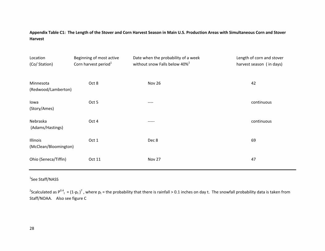
One study did assert that there is only a 20-day stover harvesting season, casting doubt on the technical feasibility of stover harvest (Petrolia). Apparently, this statement is based on the time that a corn harvesting crew in Redwood County Minnesota has between the end of the most active corn harvesting period, November 8, and the date when the probability of a week without snow falls below 40 percent, November 26 (see appendix C). Another important area where standard corn harvest crews would be impeded by early snowfall is Seneca County, Ohio. Otherwise, comparable snowy weather tends to come a month later in the dominant production area of Illinois. And enough clear weather is likely in production areas of Iowa and Nebraska, so harvest could likely proceed throughout the winter with the existing organization of corn harvest crews. Lastly, harvest crews will likely reorganize with more labor to accomplish simultaneous harvest of corn if it is necessary. Then the stover harvest season would extend to include the entire corn harvest period - above 43 days in Minnesota and Ohio, and up to 75 days in central Illinois (appendix C).

Storage and handling costs are included in a fashion that is consistent with CIF plant pricing in an established competitive market. That is, handling, shipping and storage costs are calculated and added to farm costs as if the farmer transfers ownership after he performs these functions. We do use the price semi-truck services and the rental of a storage building, then adjust capacity to apply to stover; farmers routinely purchase these services when marketing commodities. Producer cost could be further lowered if they integrate backwards to perform these functions, too.

It is useful to separate cost estimation from profit margins to the extent possible. First, the supply curve for a competitive relies on the marginal cost, ie, the break-even price for the marginal producer. Second, FOB firm pricing may well be monopsonistic (Gallagher, Wisner and Brubacker, p. 123). Here, monopsonistic pricing could evolve with processors or their middlemen providing transport, harvest, and handling services to the farmer. Calculations of farm cost and handling services will indicate when competition or a cooperative might be viable.

Farm Cost Estimates  

Revised cost estimates reflect today’s technology and input cost environment. Updated information is used for the variables hi, Ysn, and the fertilizer and fuel prices that define stover harvest costs.

The corn stover cost estimates of table 2 refer to 2011 input prices in Story County, Iowa, an important production region. Fixed and variable costs for the main harvest activities, chop, rake, and field transportation are included. Also, fertilizer replacement for the soil nutrient loss in stover harvest is valued at 2011 fertilizer prices. Hired labor costs for the stover harvesting activities is now included, because peak harvesting period labor is more likely to constrain owner’s labor when a stover enterprise is added.2 In comparison to the earlier study using this method, the overall Farm cost estimate, $32.71/ton, has doubled due to increasing energy and fertilizer prices. But corn stover does remain the lowest cost biomass source in the Midwest.

    

15  

Also, the parameters for the farm cost function are defined in table 2.

The ton-constant costs , βf = 18.37, are the sum of field hauling and fertilizer replacement costs. The acre-constant costs, αf = 36.72 , includes rake chop, bale and labor costs. Overall farm costs are ton-constant costs + acre-constant costs divided by net stover yield. Net Stover yield is Ysn=2.72 ton/acre for Story County, Iowa.

Lastly, let us demonstrate the important role of harvested stover yield in Stover costs (per ton). Consider the case where Ysn=0.95 (Hildalgo County, Texas). Then, using the farm cost function, overall Stover costs are Cst=$58.46/ton. Comparing Story County and Douglas County, costs per ton increase by 60 percent because many of the same operations are conducted on the same land because the yield is reduced by 65 percent.

Handling Costs  

Handling costs include expenditures for loading the bales that are stored in the corner of the farmer’s field onto the truck, expenditures for the truck’s trip to the processing plant, and stover storage, say near the plant.

Handling costs can vary widely according to location, length of run, and assumptions about marketing technology. First, the northwest section of the stover harvest belt likely requires storage during a snowy winter, but elsewhere, stover recovery could match processing needs and avoid storage. Second, analyses of the “first plant” typically have very high transport costs because producer participation is low and trucks have to travel great distances to secure input supplies. In contrast, established markets will likely follow the S-shaped adoption curve with very high farmer participation rates. Third, “first plant” analyses have a tendency to use capital expenditure analyses for new equipment. These analyses tend to overestimate costs; sometimes a useful asset life from the tax tables is used while equipment really lasts longer; the tax advantages of equipment leasing are not recognized; and sometimes these estimates are over capitalized by imposing investments on every farm that may ultimately match the local processing capacity.

Handling Cost Estimates 

Our handling costs assumptions are designed for a resource assessment; high farmer participation is high; and rental rates for marketing services are used. Farmers usually purchase product transport, storage and labor services, so we combine market rental rates and input requirements for handling cost estimates.

The estimate for field-loading the truck is $0.78/ton. The underlying machinery cost estimate is $33.46/hr for variable (fuel and repair) cost of farm machinery (ISU extension bulletin PM-710, estimating farm machinery costs). The physical input factors are 26 bales / truck and 0.5 hour/truck.

The estimate for truck transport to plant is $2.33/ton. This estimate is based on a formula for the average delivered transport cost for a processing plant (Gallagher and Johnson, p. 117). The formula gives average transport cost (ATC) is a function of the market transport charge (t) and the radius of the market area ( r ) :                                                                              

        ATC  = 2/3 * t *   r                                                                                      

In turn the market area times the density of corn equals the plant capacity (Q). So the radius of the market

    

16  

area is defined by the condition:  

          / ,                                                                                   

where d is the density of stover (in acre/mi2) and Yn is the net stover yield (in tons/acre). The market is defined by a 25 MGY biomass ethanol plant. But the size of the market area varies across counties because the stover yield and corn density vary. We assume that 100 percent of the corn area that can have sustainable stover harvest is actually used. A typical value is d=235 acre stover / sq. mi. In effect, we estimate transport costs in a well-developed industry. 3

3Others have estimated startup cost for the first plant locating in an area with a new technology, with participation rates as low as

20% (Perlak and Turhollow, p.1401). Then d=0.20*235 acre / mi2.

The market rate for local trucking services, t=$0.14/ton/mile, is converted from a rate per truck quote, using the loading factors one truck/26 bale and 1.2 bales / ton. The truck rate of $3.00/mile/truck comes from a survey (ISU extension custom rate survey, 2011).

The input market area required to supply a 25 MGY biomass ethanol plant defines an estimate of r=25 miles.

The estimate for stover storage cost is $3.44/ton. This estimate is calculated from a market rate of machine storage estimate of $0.30/ft2/yr (ISU extension Farm Building Rental Survey, 2010). The input requirement is a biomass storage density of 11.25 ft2/ton. Also, a biomass Storage loss of 2 percent / year is assumed.

Handling costs vary across counties with local input supply areas because r varies with the density of biomass supply in the local input market. For the example above:

Total handling costs = field haul + truck to plant + storage =0.78 + 2.33+ 3.44 =$6.55/ton

But counties with low density corn supplies would have higher average handling costs. The formula giving the relation between corn density and transport cost is given in Gallagher and Johnson.

Delivered Plant Cost 

Delivered Plant cost is the sum of farm cost, transport and storage. The Figure 4 shows the spatial distribution of delivered plant cost for the short list of counties. Throughout the interior cornbelt, delivered plant cost converts to a biomass cost in ethanol production of $.50/gallon or less. The higher cost counties, in the $.50/gal to $.75/gal range, are all on the outer boundary. Higher delivered costs result from a combination of factors, such of higher conservation allowances where wind erosion becomes a factor, and lower density of corn plantings.

    

17  

Table 2. Corn Stover Harvest Cost Details

story county corn yield 161.4 (bu/acre)

harvest index 0.515281

gross  stover yield 6861.2 (dw lb/ac) 3.43 dwt/acre

conservation 1430.0 (dw lb/ac) 0.72 (dwt/acre)

net stover yield 5431.2 (dw lb/ac) 2.72 (dwt/acre)

Direct Harvest Costs

operation fixed cost             variable cost total

reported per ton s reported per ton s cost

chop 4.0 ($/acre) 1.472979 ($/ton) 3.5 ($/acre) 1.289 ($/ton s)

bale 7.7 ($/acre) 2.835484 ($/ton) 4.5 ($/acre) 1.657

haul 1.40000 ($/ton) 1.700

5.708463 ($/ton) 4.646 10.35

Fertilizer Replacement Costs

    ferti l izer application rates            ferti l izer price fertil izer

gross dilute strength pure expense

(t f/ dwt s) $/ton f) ($/ton f) ($/ton s)

p2o5 0.001604 509 0.45 1131.111 1.814302

k2o 0.012227 511 0.6 851.6667 10.41333

NH3 0.008093 398 1 398 3.221014 15.45

Hired Labor Costs

labor requirement 1.33 hr/acre wage 12.8 $/hr 6.27

Total Farm Costs For Owner-Operator 32.07

Cst = 18.55 + 36.72 / Ysn costs  constant per

acre 36.72

ton 18.55

Ysn 2.72

Farm owner-operator cost w/ hired labor $/tn 32.07

    

18  

Figure 6.

 

   

    

19  

U.S. Stover Supply Schedule  

The corn stover supply curve for the United States is shown in figure 6.  The supply schedule is 

calculated by sorting the short list of counties by delivered cost and cumulating for the stover supply, or 

production less feed demand, at each price.  Also, feed use of stover is added to industry supply when 

the price exceeds the livestock feed value.  

Inspection reveals that the lowest entry price is about $37.5/ton.  Further, 100 mill. Mt would be 

available at a slightly higher supply price of $40.4/ton.  Beyond that, the supply schedule becomes 

steeper to attract supplies from low density supply areas and supplies in feed use; 117 million tons 

would be available at a supply price of $59.7/ton.  Also, the supply schedule becomes vertical at the 

point, $62.9/ton and 133 million tons, the point where forage use is converted to industry supply. 

Conclusions  

Previous estimates suggested that accessible and sustainable corn residue supplies are adequate for a  

new biomass processing industry.  Revision is justified now because the agronomic and economic 

environment has changed.  Also, there is an interest in the location of low cost biomass supplies. 

 The revised estimates of corn stover cost and supply fit today’s yield and input situation.  The revised 

estimates confirm that corn stover supplies could be a low cost feedstock for a low cost and extensive 

bioenergy industry.  Supplies of 100 million metric tons of stover would be available to an established 

industry at a delivered plant price between $37.5/ton and $40.5/ton.   At moderately higher prices, the 

feedstock for a 10.5 MGY ethanol industry would be available.  Several offsetting changes in economic 

environment and technology have occurred since we calculated our first estimates, but the new supply 

estimate is still slightly larger.  Stover cost remains highly competitive in today’s energy market.   

Ample supplies of the lowest cost and sustainable supplies are likely found in the middle of the corn‐ 

belt: Illinois, Indiana, Eastern Ohio, and Iowa.  Also, sections of other states have some very low‐cost 

supplies: eastern Nebraska, southern Minnesota, southern Wisconsin, and southern Michigan.  Lastly, 

considerable stover supplies would be available at a somewhat higher but still very competitive price in 

some new cornbelt areas: eastern North Dakota, central Wisconsin/Michigan, and perhaps western New 

York. Supply estimates for specific counties are given in appendix B.  

   

    

20  

 

 

 

  

20

30

40

50

60

70

80

90

0 10 20 30 40 50 60 70 80 90 100 110 120 130 140

Supply Price (Delivered PLant Cost, in $/ton

Quantity,  in million tons

Figure 6. U.S. Corn Stover Supply

    

21  

References

Al-Kaisi, M.M., X. Yin, M.Hanna, M.D.Duffy, Resources Conservation Practices: Considerations in Selecting No-Till, Iowa State University Extension Service, PM 1901d, July 2009.

D.A. Angers, “Changes in Soil Aggregation and Organic Sarbon under Corn and Alfalfa”, Vol. 56 No.4, July-August 1992:1,244-1,248.

Atchison, J.E. and J.R. Hettenhaus, Innovative Methods for Corn Stover Collecting, Handling, Storing and Transporting, National Renewable Energy Laboratory, NREL/SR-510-33893, April 2004.

John M. Baker, Tyson E Oshsner, Rodney T. Venterea, Timothy J. Griffis, “Tillage and Soil Carbon Sequestration-What do we really know?” Agriculture Ecosystems and Environment 118 (2007):1-5.

Clay D, Carlson G, Schumacher T, Owens V. Mamani-Pati F, Biomass estimation approach impacts on calculated soil organic carbon maintenance requirements and associated mineralization rate constants” J. Environ. Qual 39:784-790 (2010).

C.J. Dell, P.R. Salon, C.D. Franks, E.C. Benham, and Y. Plowden, “ No-till and cover crop impacts on soil carbon ans associated properties on Pennsylvania dairy farms” Journal of Soil and Water Conservation, May/June 2008-Vol.63,No.3: 136-142.

Edgerton, Mike, “Corn Stover: A part of the Carbon budget,” presentation at the 2010 Corn Technology Workshop, Aug 30, 2010, Ankeney, Iowa.

Gallagher, P., M. Dikeman, J. Fritz, E. Wailes, W. Gauthier, and H. Shapouri, “Supply and Social Cost Estimates for Biomass from Crop Residues in the United States,” Environmental and Resource Economics 24 (April 2003):335-358.

Gallagher, P., R. Wisner, H. Brubaker, “Price Relationships in Processors’ Input market Areas: Testing Theories for Corn Prices near Ethanol Plants,” Canadian Journal of Agricultural Economics 53(2005):117-139.

Gallagher, P., M. Dikeman, J. Fritz, E. Wailes, W. Gauthier, and H. Shapouri, Biomass from Crop Residues: Cost and Supply Estimates. U.S. Department of Agriculture, Office of the Chief Economist, Office of Energy Policy and New Uses, Agricultural Economic Report No. 819 (2003).

Gallagher, Paul and Donald L. Johnson, “Some New Ethanol Technology: Cost Competition and Adoption Effects in the Petroleum Market,” The Energy Journal 20 (April1999):89-120.

Graham, R.L., R. Nelson, J. Sheehan, R.D. Perlack and L. L. Wright, “Current and Potential US Corn Stover Supplies,” Agronomy Journal 99 (2007):1-19.

Perlak, R.D., and A.F. Turhollow, “Feedstock cost analysis of corn stover residues for further processing,” Energy 28 (2003):1395-1403.

Petrolia, Daniel R., “An Analysis of the Relationship between Demand for Corn Stover as an Ethanol Feedstock and Soil Erosion” Review of Agricultural Economics 30 (2008):677-692.

    

22  

Sheehan, J., A. Aden, K. Paustian, K. Killian, J. Brenner, M. Walsch, and R. Nelson, “Energy and Environmental Aspects of Using Corn Stover for Fuel Ethanol,” Journal of Industrial Ecology 7 (2004):117-146.

Shroyer, J.R., K.C. Dhuyvetter, G.L. Kuhl, D.L. Fjell, L.N. Langemeier, J.O. Fritz, Wheat Pasture in Kansas, Cooperative Extension Service, Kansas State University, Manhattan, C-173, April 1993.

Staff, Ag Decision Maker: 2011 Iowa Farm Custom Rate Survey, Iowa State University Extension Service FM 1698, March 2011.

Staff, Ag Decision Maker: Iowa Farm Building Rental Rate Survey, Iowa State University Extension Service, FM 1838, January 2010.

Staff, Ag Decision Maker: Estimating Farm Machinery Costs, Iowa State University Extension Service, PM-710, November 2009.

Staff, Ag Decision Maker: Estimated Costs of Crop Production in Iowa, Iowa State University Extension Service, FM 1712, December 2009.

Staff, Ag Decision Maker: Estimating Farm Machinery Costs, Iowa State University Extension Service, PM-710, November 2009.

Staff, National Soil Survey Handbook, National Resources Conservation Service, July 14, 2011, http://soils.usda.gov/techincal/handbook/.

Staff/NOAA, Daily Probabilities of Receiving Snowfall Beyond the Specified Thresholds, NOAA Satellite and Information Service, http://www.ncdc.noaa.gov/ussc/USSCAppController?action=shofall_prob_daily&state, May 2012.

Staff/NASS, Field Crops Usual Planting and Harvesting Dates, U.S. Dept of Agriculture, National Agricultural Statistics Service, Agricultural Handbook Number 628, October 2010.

WIlhelm, W.W., JMF Johnson, Douglas L Karlen, and Davit T. Lightle, “Corn Stover to Sustain Soil Organic Carbon Further Constrains Biomass Supply,” Agronomy Journal (2007): vol. 99,No.6: 1665-1667.

D.R. Wiggins, J.W. Singer, K.J. Moore, and Kendall R. Lamkey, “Maize Water Use in Living Mulch Systems with Stover Removal,” Crop Science 52 (2012):327-338.

    

23  

Appendix A:  Stover Harvest and Soil Carbon Maintenance 

 

Soil Organic Carbon is an important quality indicator that defines the long term productive potential of a plot of land. There are several strategies available for maintaining SOC. There are also several relevant externalities associated with bio-fuel production, and each SOC maintenance strategy makes a distinct contribution to the set of externalities. Eventually, SOC strategies should be evaluated as a constraint in a market context that includes the entire set of externalities.

Methods of Soil Carbon Control 

There are three approaches to maintaining SOC while planting corn and harvesting stover. Now we review these techniques, and the advantages and disadvantages.

One approach it to restrict or eliminate corn stover harvest on the notion that some of the stover left on the ground will decompose and turn to soil carbon. Wilhelm, et al, provide the reference study for this approach. To illustrate their results, use the story county, Ia corn yield of Yc=161.4 bu/acre (from the cost table) and notice that the gross stover yield is Ysg= 3.43 ton/acre. Using Wilhelm, et al’s table 1b with the conservation tillage assumption, the allowable stover harvest is 0.73 ton/acre. Using results from this reference study, the stover harvest rates are likely so low that harvesting is not worth it.

But the below-ground biomass that grows with the corn plant may be higher than Wilhelm, et al assumed. Baker, et al argued that the root/shoot ratio (R/S) is higher than many thought. Further, recent measurements by seed companies with their newest varieties gave a root shoot ratio of R/S= 0.55 (Edgerton, et al).

To illustrate the effect of a higher R/S on allowable stover harvest, consider an estimated relationship (Clay, p.787 ) between the percentage of corn stover that can be harvested for SOC maintenance( H ) and R/S:

 H = 34.6 + 39.4 R/S.  So H=56.3 when R/S=0.55.  

Continue with The Story County, Iowa example, Ysg=3.43 t/ acre. The stover harvest that would maintain SOC is Ysn = 0.55*3.43 t/ acre= 1.9 ton/acre. At harvest rates near 2 t/acre, it is more worthwhile to run harvesting equipment across the field.

A second technique for soil carbon maintenance is adding manure. In corn silage production, all of the stover is harvested with the corn while it is still green. Since corn silage is only produced on dairy farms, there is always an ample manure supply. A recent crop experiment included corn silage and measured soil organic carbon (SOC) (Dell, et al). The results showed that SOC accumulated in corn silage experiments. Also, SOC accumulated faster when conservation tillage was used.

 

   

    

24  

A third technique is to harvest corn stover at a high rate, mindful of soil erosion constraints. Periodically, the land is rotated into a perennial such as alfalfa in order to rebuild the carbon if necessary.*

This rotation approach is used in developing the estimates of this report. The rotation approach differs from the previous two techniques in that soil carbon cycles over a crop rotation period were used, instead of satisfying an annual carbon budget.

Agronomic experiments do support the rotation approach to SOC maintenance (Angers). Specifically, in a 5-year experiment, corn for silage (i.e., all residue is harvested) was grown on one set of plots continuously-there was no soil maintenance in the fall, and 6”deep tiller treatment in the spring. The second set of plots contained alfalfa that was planted in the first year and maintained through the remainder of the experiment.

Regressions for SOC observations from the corn and alfalfa plots are:

Corn:  C = 25.6 ‐0.24 X and Alfalfa: C = 29.5 – 4.62 exp[ ‐0.023*exp(1.71x} ],                             

where X=0,1,2,3,4,5 corresponding to the beginning of the experiment and each season.  

As the figure below shows, the SOC decline is slow, steady and moderate for corn. For alfalfa, not much SOC change occurs at first, but accumulations become substantial as the experiment progresses.

 

 

 

 

   

    

25  

Using the regressions above, we calculated the estimated soil carbon when alfalfa is planted first for 4 years and then followed by corn. After 19 years with corn, the SOC had returned to the initial level from before alfalfa was planted. The implication is that a farm in continuous corn with 100% stover harvest could maintain SOC could be maintained if 82.6 percent of the available land is in corn with stover harvest, and the other 16 percent of the land would be in alfalfa.

Others confirm the crop rotation approach to SOC maintenance. For instance, carbon rebuilding with alfalfa would take a few years because the relatively long carbon assimilation season for alfalfa extends into the early spring pre-planting period and late fall post-harvest period (Baker, et al). Also, the IPCC seems to share this view on crop rotation and SOC; they estimate that the equilibrium SOC level for hay is 55 percent higher than it is for cropped land (Gallagher, et al, provide a summary of IPCC estimates and references).

We did not adjust the sustainable area base in my corn stover supply calculations (fr=1.0 instead of 0.82). We need to know the “land transition matrix” from corn to hay and back to corn, in order to see if adjustments to the sustainable area base are needed. Producers could already be rotating crops in a fashion consistent with SOC maintenance. Future research and data collection could resolve this uncertainty.

A fourth technique for managing SOC in conjunction with stover harvest is the joint production of corn, stover and a living mulch (e.g., blue grass) or cover crop (e.g., clover). From preliminary results, reductions in corn yield and stover yield do occur when living mulch or cover crop are used. However, there was a living mulch treatment (blue grass) that maintained corn yields (Wiggans, et al).

External Benefits and Costs 

The four methods of controlling soil carbon (restricted stover harvest, added manure, rotated crops, and jointly planted cover crop) differ in the external benefit that they produce for society as a whole. First, there are external benefits associated with the production of biofuels: reduce Midwestern unemployment , reduce oil market disruption and disengage from middle east politics, clean air in urban areas, reduce global warming emissions. The size of these external benefits are proportional to the level of stover (and biofuel) production. Hence, the external benefit of restricted harvest is less than the external benefit of rotated crops.

Second, it is important that all carbon control methods are used in conjunction with low till methods of crop production because tillage releases soil carbon into the atmosphere, possibly aggravating global warming. All four of the SOC control methods can be combined with low-till agriculture. Perhaps policies should be revised to ensure that SOC control methods are combined with low till agriculture, if stover harvest is practiced.

Third, the added manure method may not perform with the other three methods in regards to global warming emissions, in the final analysis. But it is possible that emissions to air are reduced when manure is incorporated in soil. And careful use on cropland could reduce phosphate leaching to surface water. Lastly, the external benefits of ethanol production are usefully arranged in a hierarchy: CO2 is important, but the employment and trade disruption benefits are first order benefits. It makes sense to use 

    

26  

a SOC maintenance technique like manure addition that may not include strong performance on global warming.  

The Need for Further Economic Evaluation 

A more systematic look at opportunity costs is needed. Generally speaking, this means that an initial reference situation, or baseline, is fully defined. Then the improvement or deterioration associated with adding one of these SOC management strategies can be measured.

For instance, the baseline for U.S. agriculture likely includes a devaluing dollar and expanding livestock exports to china. The reference situation includes growing manure disposal problems. If we do not use the added manure strategy, the manure could possibly end up in the water and the air instead of the soil.

Also, a qualitative comparison of the restricted harvest and rotation is helpful. First, the annual carbon budget constraint of the restricted harvest approach is unnecessary. Restricted harvest seems like a game of ‘mother may I’ where you can only win by taking small steps forward. In contrast, the rotation strategy looks like several small steps backwards and one large step forward to get to the same end. Both approaches are pretty good wrt CO2. Second, the stover harvest costs are much higher with the restricted harvest. Using restricted stover harvest, the estimate is usually about TWICE the cost using rotation. Why? Most of the harvest costs are roughly constant on a per acre basis. Under rotation the harvest equipment travels across the same number of acres and harvests twice the amount of stover.

Lastly, it may be time to move the corn production, stover harvest, and soil maintenance to the next level of economic analysis for a systematic look at costs and benefits of the alternatives. Using the discounted Present Value Mathematical Programming setup of this problem, four different production techniques could be specified: restricted harvest, rotation, manure application, and joint cover crop. Techniques would have (i) a stream of corn outputs and stover outputs, (ii) may have a maintenance crop over the production cycle, (iii) may have a lower or higher corn yield than another technique, (iv )a set of coefficients indicating the effect on one of the external benefits. The solution to this problem could suggest that several techniques are useful, or there could be one dominant technique. The jury is still out on this one.

Until then our approach, which limits harvest to land with low erosion potential but allows high stover harvest rates, is a good candidate for the low cost method of harvesting stover that controls soil erosion and stabilizes carbon.

   

    

27  

Appendix B:  County Estimates of Stover Availability and Cost 

See:  http://www2.econ.iastate.edu/faculty/gallagher  

 

Appendix C:  Estimates of Stover Harvest Season Length 

   

    

28  

Appendix Table C1:  The Length of the Stover and Corn Harvest Season in Main U.S. Production Areas with Simultaneous Corn and Stover 

Harvest 

 

 

Location    Beginning of most active  Date when the probability of a week      Length of corn and stover 

(Co/ Station)    Corn harvest period1    without snow Falls below 40%2        harvest season  ( in days) 

           

 

Minnesota       Oct 8        Nov 26              42 

(Redwood/Lamberton) 

 

Iowa        Oct 5        ‐‐‐‐              continuous 

(Story/Ames) 

 

Nebraska      Oct 4        ‐‐‐‐‐              continuous 

 (Adams/Hastings) 

 

Illinois        Oct 1        Dec 8              69 

(McClean/Bloomington) 

 

Ohio (Seneca/Tiffin)    Oct 11        Nov 27              47 

  

1See Staff/NASS  

2Scalculated as P0.4t  = (1‐pt )7 , where pt = the probability that there is rainfall > 0.1 inches on day t.  The snowfall probability data is taken from 

Staff/NOAA.    Also see figure C  

   

    

29  

Appendix Table C2:  The Length of the Stover and Corn Harvest Season in Main U.S. Production Areas with Sequential Corn and Stover 

Harvest 

 

 

Location    End of most active    Date when the probability of a week      Length of corn and stover 

(Co/ Station)    Corn harvest period1    without snow Falls below 40%2        harvest season  ( in days) 

           

 

Minnesota       Nov 8        Nov 26              19 

(Redwood/Lamberton) 

 

Iowa        Nov 9        ‐‐‐‐‐              continuous 

 (Story/Ames) 

 

Nebraska      Nov 10        ‐‐‐‐‐‐              continuous 

 (Adams/Hastings) 

 

Illinois        Nov 5        Dec 8              34 

(McClean/Bloomington) 

 

Ohio (Seneca/Tiffin)    Nov 20        Nov 27              7 

  

1See Staff/NASS  

2Scalculated as P0.4t  = (1‐pt )7 , where pt = the probability that there is rainfall > 0.1 inches on day t.  The snowfall probability data is taken from 

Staff/NOAA.    Also see figure C 

 

   

    

30  

 

0.00

0.10

0.20

0.30

0.40

0.50

0.60

0.70

0.80

0.90

1.00

30‐Sep 7‐Oct 14‐Oct 21‐Oct 28‐Oct 4‐Nov 11‐Nov 18‐Nov 25‐Nov 2‐Dec 9‐Dec 16‐Dec 23‐Dec 30‐Dec 6‐Jan 13‐Jan 20‐Jan 27‐Jan

mn (redwood)

ia(story)

ne(adams)

il(McClean)

oh (seneca)

Figure C. The probability of a week without snowfall  at major stover harvest locations1

state(county):

1 data shown are 5‐day centered moving averages,  Pt =  (1/12) pt‐2 +(1/6) pt‐2 +pt +(1/6) pt‐+1+(1/12) pt+2of the calculated probability for a particular day( pt‐+i )