university of brasilia post graduation program in ... · post graduation program in chemistry...
TRANSCRIPT

UNIVERSITY OF BRASILIA
POST GRADUATION PROGRAM IN CHEMISTRY
RECONSTRUCTION OF NEOGENE SEA SURFACE
TEMPERATURES IN CEARA RISE (SOUTH ATLANTIC)
BASED ON ALKENONES
Juliana Pinheiro Pires
Supervisors:
Prof. Dr. Fernanda Vasconcelos de Almeida
Dr. Jung-Hyun Kim
Brasilia – DF
2015

i
JULIANA PINHEIRO PIRES
RECONSTRUCTION OF NEOGENE SEA SURFACE TEMPERATURES IN
CEARA RISE (SOUTH ATLANTIC) BASED ON ALKENONES
Dissertation submitted to the Institute
of Chemistry, University of Brasilia,
as a partial requirement for obtaining
title of Master in Chemistry.
Area of concentration: Analytical
Chemistry.
Supervisors: Prof. Dr. Fernanda
Vasconcelos de Almeida and Dr. Jung-Hyun Kim.
Brasilia - DF
2015

ii
APPROVAL SHEETF
Communicate the approval of the Dissertation Defesnse of Master
of the student Juliana Pinheiro Pires, registration nº. 13/0086053, entitled
"Reconstruction of Sea Surface Temperatures Neogene In Ceara Rise
(South Atlantic ) Based On Alkenones " presented at PADCT room of the
Institute of Chemistry ( IQ ) of the University of Brasilia ( UnB ) on March 5,
2015 .
Prof. Dr. Fernanda Vasconcelos de Almeida
President of the sink (IQ/UnB)
Prof. Dr. Valéria Regina Bellotto
Titular Member (IQ/UnB)
Prof. Dr. Poliana Dutra Maia
Titular Member (FUP/UnB)
Prof. Dr. Marly Eiko Osugi
Substitute Member (IQ/UnB).
March 5, 2015

iii
I dedicate this thesis to my parents Roberto and Maria Geralda,
who gave me unconditional support and do not measure efforts to
the realization of my dreams.
Dedico essa dissertação aos meus pais Roberto e Maria Geralda,
pelo apoio incondicional e por não medirem esforços para
a realização dos meus sonhos.

iv
ACKNOWLEDGMENTS
Thank first to God for giving me strength and wisdom to walk the paths of
graduation and master and overcome the difficulties.
To my parents, who were with me in the moments that I most needed and
advised me in the most difficult moments. You are responsible for the person I
have become. I love you.
To my sister Luciana and my boyfriend Jonatan, who endured my moments of
anxiety and stress. Without the love, friendship and fellowship of you, I could not
conclude this important stage of my life.
To the teacher Dr. Fernanda, who welcomed me in the laboratory and was
always willing to listen and help me. Thank you for being my supervisor and
giving me all the support necessary for the conclusion of this master.
To my supervisor Dr. Jung- Hung Kim, for sharing her experience and wisdom.
To Elsbeth Van Soelen, for all patience, attention and dedication and for being
my partner in all stages of this master. Thank you.
To the AQQUA teachers, Valéria, Jez, Fernando, Ana Cristi and Alexandre, for
being always available to help and answer questions.
To my colleagues in AQQUA Group, especially Angela, Gabriel, Tati, Rosy,
Carla, Victor, Milena and Daniel, for sharing great moments of relaxation, laugh
and for be always willing to help me.
To CNPq, for financial support.
To the ClimAmazon Project for financial support.
To UNB and the Institute of Chemistry.
And to all who were part of this history.
Thank you!

v
AGRADECIMENTOS
Agradeço primeiramente a Deus, por ter me concedido força e sabedoria para
trilhar os caminhos da graduação e do mestrado e vencer as dificuldades.
Aos meus pais, que estiveram ao meu lado nos momentos que mais precisei e
me aconselharam nos momentos mais dificeis. Vocês são os responsáveis pela
pessoa que me tornei e devo aos dois tudo que já consegui. Amo vocês.
À minha irmã Luciana e ao meu namorado Jonatan, que aguentaram meus
momentos de ansiedade e de estresse. Sem o carinho, a amizade e o
companheirismo de vocês, eu não conseguiria concluir esta etapa tão importante
de minha vida.
À professora Dra. Fernanda, que me acolheu no laboratório e sempre esteve
disposta a me ouvir e ajudar. Obrigada por ser minha orientadora e me dar todo o
suporte para que esse mestrado se realizasse.
À minha coorientadora Dra. Jung-Hung Kim, pela experiência e sabedoria.
À Elsbeth Van Soelen, por toda paciência, atenção e dedicação e por ser minha
companheira em todas as etapas dessa dissertação. Muito obrigada.
Aos professores do AQQUA, Valéria, Jez, Fernando, Ana Cristi e Alexandre, por
estarem sempre dispostos a ajudar e tirar dúvidas.
Aos colegas do Grupo AQQUA, especialmente Angela, Gabriel, Tati, Rosy,
Carla, Victor, Milena e Daniel, por proporcionarem ótimos momentos de
descontração, boas risadas e estarem sempre dispostos a me ajudar.
Ao CNPq e ao Projeto ClimAmazon, pelo auxílio financeiro.
À UnB e ao Instituto de Química.
E a todos que fizeram parte dessa história.
Muito Obrigada!

vi
“The real voyage of discovery consists not in seeking new landscapes, but in
having new eyes.”
Marcel Proust
“A verdadeira viagem de descobrimento não consiste em procurar novas
paisagens, mas em ter novos olhos.”
Marcel Proust

vii
ABSTRACT
PIRES, J. P. Reconstruction of Neogene sea surface temperatures in Ceara
Rise (South Atlantic) based on alkenones. 2015. Dissertation (Master in
Chemistry) – University of Brasilia, Brasilia, 2015.
The Ceara Rise is a seismic peak located in the Atlantic Ocean and
receives both marine and terrigenous sediments. These sediments are
important for understanding the paleoclimatic and paleo-environmental
conditions in the ocean. With the goal of reconstructing the past sea surface
temperature (SST), the lipid biomarkers n-alkanes and alkenones were
analyzed in sediments of Ceara Rise. The quantification of both biomarkers was
performed by Gas Chromatography with Flame Ionization Detector (GC-FID).
For the n-alkanes, analytical curves, which resulted in acceptable figures of
merit by official norms and the National Institute of Metrology, Quality and
Technology(Inmetro) were built. Because there is no alkenone standard
commercially available for the construction of analytical curves for alkenones,
the quantification was done by comparison of the areas of analytes to the area
of a standard ketone commercially available. The quantification by comparison
areas was validated by T-Test, in which the values of concentration of n-alkanes
obtained for this quantification method were compared with the calculated
concentrations from analytical curves, which led to satisfactory results. The
n-alkanes were evaluated according to the proxies Carbon Preference Index
(CPI) and Average Carbon Length (ACL). The results suggest that the main
source of organic matter in the studied sediments originates from terrigenous
material transported by rivers and by wind action. The , proxy that use the
concentration of alkenones to calculate the SST, was used for climatic
reconstruction of the region. The concentration range of alkenones was 0.001 to
0.516 µg g-1. According to the result of proxy, the estimated lowest
temperature was 22.5 °C, toward the end of Early Miocene, while the highest
temperature, 28.5 ° C, was held at half the Early Oligocene.
Keyword: Ceara Rise, Sediments, CPI, ACL, and SST

viii
LIST OF FIGURES
Figure 1. Structure of methyl (Me) and ethyl (Et) long-chain alkenones. The
position of the double bounds are indicated by red circles. Adapted from
CASTAÑEDA et al., 2008............................................................................... 20
Figure 2. Illustration of the SST proxy. On the left, gas chromatogram of a
sample with relatively cooler signal than the chromatogram on the right.
Adapted from CASTAÑEDA et al., 2008. ....................................................... 21
Figure 3. Location of Ceara Rise in the Atlantic Ocean. Adapted from CURRY
et al., 1994..................................................................................................... 24
Figure 4. Structural map of the equatorial Atlantic and of the boundaries of the
Ceara Rise and Sierra Leone Rise, from KUMAR et al., 1977. ...................... 25
Figure 5. Pesperctive view of Ceara Rise, ODP 154, site 925. Adapted from
CURRY et al., 1994. ....................................................................................... 28
Figure 6. Extracts of sediment samples from Ceara Rise.............................. 32
Figure 7. (A) Sodium sulfate column prepared in a Pasteur pipette and (B)
system to transfer the extract to the vial through the column. ........................ 33
Figure 8. General scheme of the analytical work flow. .................................. 35
Figure 9. Gas chromatography with flame ionization detector (GC-FID) Agilent
7650A. ............................................................................................................ 37
Figure 10. Recovery factors (%) of rotoevaporation and concentration steps of
the solvent with a nitrogen flow. ..................................................................... 46
Figure 11. Comparing the concentrations obtained for different number of
extractions of alkenones……………………………………………………….…..46
Figure 12. Comparing the concentrations obtained for different number of
extractions of n-alkanes…………………………………………………… ... ……46
Figure 13. Typical chromatogram obtained for n-alkanes extracts (sample CRA
5 R4). ............................................................................................................. 50
Figure 14. Analytical curve of C-22............................................................... 52
Figure 15. Analytical curve of C-23............................................................... 52
Figure 16. Analytical curve of C-24............................................................... 52

ix
Figure 17. Analytical curve C-25................................................................... 52
Figure 18. Analytical curve of C-26............................................................... 52
Figure 19. Analytical curve of C-27............................................................... 52
Figure 20. Analytical curve of C-28............................................................... 53
Figure 21. Analytical curve of C-29............................................................... 53
Figure 22. Analytical curve of C-30............................................................... 53
Figure 23. Analytical curve of C-31............................................................... 53
Figure 24. Analytical curve of C-32............................................................... 53
Figure 25. Analytical curve of C-33............................................................... 53
Figure 26. Analytical curve of C-34............................................................... 54
Figure 27. Analytical curve of C-35............................................................... 54
Figure 28. Representative chromatogram of sediment sample containing
alkenones. ...................................................................................................... 64
Figure 29. Calculated CPI values along the record at sites 925 A and 925 B,
situated at Ceara Rise. ................................................................................... 70
Figure 30. ACL values calculated over the record sites 925 A and 925 B,
situated at Ceara Rise. ................................................................................... 71
Figure 31. Alkenone derived sea surface temperature (°C) record at sites 925 A
(represented in red) and 925 B (in blue), situated at Ceara Rise. .................. 72

x
LIST OF TABLES
Table 1. Information about the Core Recovery A (CRA): period, age, sample´s
name and depth. ............................................................................................ 29
Table 2. Information about the Core Recovery B (CRB): period, age, sample´s
name and depth. ............................................................................................ 30
Table 3. Basic information of the studied exploration core............................. 31
Table 4. Information about the standard used to make the analytical curve. . 36
Table 5. Chromatographic parameters of the GC-FID used in the determination
of alkenones and n-alkanes........................................................................... 38
Table 6. Values of correlation coefficients obtained from the analytical curves.42
Table 7 Estimation of SD and CV to the standards of squalene and
nonadecanone through the repeatability of areas (in picoampere (pA)). ........ 43
Table 8. Values of T-calculated for the average comparison test. ................. 45
Tabela 9. LOD and LOQ obtained for nonadecanone and squalene. ............ 48
Table 10.Retention times (min) of n-alkanes used in the construction of
analytical curve……………………………………………………………………...49
Table 11. Concentrations (µg mL-1
) and total areas of the external standard
analytical curve of n-alkanes used………………………………..………….…...50
Table 12. Weight and sediment concentrations (µg mL-1
) of 14 n-alkanes in the
sediment samples of the cores CRA and CRB of Ceara Rise obtained by
interpolation in the analytical curves............................................................... 56
Table 13. Concentrations (µg mL-1
l) of n-alkanes in 14 samples of sediment
cores CRA and CRB of Ceara Rise obtained by comparison with the area of the
internal standard............................................................................................ 60
Table 14. Concentrations (µg mL-1
) of alkenones in sediment samples of cores
CRA and CRB of Ceara Rise obtained by comparison with the area of the
internal standard............................................................................................ 65
Table 15. Concentrations (µg mL-1) of alkenones in sediment samples of cores
CRA and CRB of Ceara Rise obtained by comparison with the area of the
internal standard…………………………………………………………..………..65

xi
LIST OF ABBREVIATIONS AND ACRONYMS
ANVISA National Health Surveillance Agency
ACL Average Chain Length
AQQUA Grupo de Automação, Quimiometria e Química Ambiental
Be Berilium
C-22 N-docosane
C-23 N-tricosane
C-24 N-tetracosane
C-25 N-pentacosane
C-26 N-hexacosane
C-27 N-heptactosane
C-28 N-octacosane
C-29 N-nonacosane
C-30 N-triancontane
C-31 N-hentriacontane
C-32 N-dotriacontane
C-33 N-titriacontane
C-34 N-tetratriacontane
C-35 N-pentatriacontane
C37:2 Alkenone with 37 carbons and two unsaturations
C37:3 Alkenone with 37 carbons and three unsaturations
C37:4 Alkenone with 37 carbons and four unsaturations
C38:2 Alkenone with 38 carbons and two unsaturations
C38:3 Alkenone with 38 carbons and three unsaturations
CRA Core Recovery A
CRB Core Recovery B
CO2 Carbon Dioxide
CV Coefficient of Variation
CPI Carbon Index Preference
DCM Dichloromethane

xii
DSDP Deep Sea Drilling Project
Et Ethyl
FID Flame Ionization Detector
GC Gas Chromatograph
GDGT Glycerol Diakyl Glycerol Tetraethers
ICH International Conference of Harmonization
INMETRO Instituto Nacional de Metrologia, Qualidade e Tecnologia
IS Internal standard
KYR Thousand years
LOD Limit of Detection
LOQ Limit of Quantification
Ma Million Years Ago
mbsf Meters below sea floor
Me Methyl
MeOH Methanol
Na2SO4 Sodium Sulfate
N2 Nitrogen gas
NOAA National Oceanic and Atmospheric Administration
ODP Ocean Drilling Project
OLR Out of Linear Range
pA Picoampere
R Correlation Coefficient
RT Retetion Time
SD Standard of Desviation
SST Sea Surface Temperature
TLE Total Lipid Extract
UCM Unresolved Complex Mixture
UnB Universidade de Brasília
Unsaturation Ketone Index

SUMARY
1. INTRODUCTION .............................................................................................. 15
2. BIBLIOGRAPHIC REVIEW............................................................................... 17
2.1 CENOZOIC CLIMATE EVOLUTION.......................................................... 17
2.3. PROXIES CARBON PREFERENCE INDEX AND AVERAGE CHAIN
LENGTH AND SOURCE OF N-ALKANES ....................................................... 22
2.4. STUDY AREA............................................................................................ 24
2.4.1. PREVIOUS WORK ................................................................................. 26
3. MATERIALS AND METHODS .......................................................................... 28
3.1. SAMPLE COLLECTION AND PREPARATION ............................................ 28
3.2. ORGANIC GEOCHEMISTRY ....................................................................... 31
3.2.1. CLEANING GLASSWARE...................................................................... 31
3.2.2. LIPID EXTRACTION AND PURIFICATION ............................................ 31
3.2.2.1. EXTRACTION OF ALKENONES AND N-ALKANES ........................... 32
3.2.2.2. PREPARATION OF INTERNAL STANDARDS ................................... 33
3.2.2.3. SEPARATION OF FRACTIONS OF ALKENONES AND N-ALKANES 33
3.2.3. DETERMINATION AND QUANTIFICATION OF ALKENONES.............. 35
3.2.4. DETERMINATION AND QUANTIFICATION OF N-ALKANES ............... 36
3.3. VALIDATION................................................................................................ 38
3.3.1. DETERMINATION OF OUTLIERS IN ANALYTICAL CURVES .............. 38
3.3.2. LINEARITY ............................................................................................. 39
3.3.3. REPEATABILITY TEST .......................................................................... 39
3.3.4.T TEST FOR COMPARISON OF CONCENTRATIONS .......................... 39
3.3.5. RECOVERY TESTS ............................................................................... 40
3.3.6. LIMITS OF DETECTION AND QUANTIFICATION ................................. 41
4. RESULTS AND DISCUSSION ............................................................................ 42
4.1. METHOD VALIDATION ................................................................................ 42
4.1.1. VERIFICATION OF OUTLIERS.............................................................. 42
4.1.2. LINEARITY ............................................................................................. 42
4.1.3. REPEATABILITY .................................................................................... 43

4.1.4. T TEST FOR COMPARISON OF CONCENTRATIONS ......................... 44
4.1.5. RECOVERY TESTS ............................................................................... 46
4.1.6. LIMITS OF DETECTION AND QUANTIFICATION ................................. 48
4.2. QUALITATIVE DETERMINATION OF N-ALKANES ..................................... 48
4.3. QUANTITATIVE DETERMINATION OF N-ALKANES .................................. 51
4.4. QUALITATIVE DETERMINATION OF ALKENONES ................................... 64
4.5. QUANTITATIVE DETERMINATION OF ALKENONES ................................ 65
4.6. PROXIES CARBON PREFERENCE INDEX AND AVERAGE CHAIN
LENGTH .............................................................................................................. 69
4.7. RECONSTRUCTION OF SST ...................................................................... 71
5. CONCLUSIONS .................................................................................................. 75
6.BIBLIOGRAPHIC REFERENCE .......................................................................... 77
APPENDIX .............................................................................................................. 81

15
1. INTRODUCTION
Studies based on past climate change are frequently used to understand
current climates trends and also making forecasts. The main climate data refer to rainfall patterns and temperature variations (VILLALBA et al., 2009).
The tools proxies are equations that relate proportions of molecules with
different environmental conditions. They play an important role in the reconstruction of temperature profiles and are widely used in paleoenvironmental studies as a natural register of environmental changes (CASTAÑEDA et al.,2008; MANN et al., 2008). Among the various proxies applied to achieve this goal, those using organic molecules considered biomarkers have shown great potential for application in determining the surface temperature of the sea.
The determination of sea surface temperature (SST) is one of the
fundamental parameter for the reconstruction of past climate conditions, as well as for understanding the hydrological cycle and wind systems. (EGLINTON et al., 2008).
Considering these aspects, the present study aims to evaluate the
temperature changes on sediment core from the Ocean Drilling Program (ODP) 154, site 925 using lipid biomarkers. Site 925 sediment samples were retrieved in the Ceara Rise (South Atlantic), located 800 kilometers east of the mouth of Amazon River. The sediments contain organic matter derived from both terrestrial and marine sources. Therefore, core site 925 will provide valuable information which can help to link paleoenvironmental and paleoclimatic conditions on land to those in the ocean.
This study is part of the international project CLIM-AMAZON, the joint
Brazilian-European research facility for climate and geodynamic research on the Amazon River basin sediments. The main objectives of this project were:

16
i. to set up the analytical structure for the extraction and analysis of
lipid biomarkers in sediment samples in the analytical chemistry laboratory at the Chemistry Institute in the University of Brasilia (UnB), AQQUA group;
ii. to analyze n-alkanes and alkenones, two types of lipid biomarkers,
in marine core sediments of Ceara Rise (South Atlantic) at different core depth levels;
iii. to generate analytical data for reconstruct the past sea surface
temperatures from the Miocene to the Holocene in the Ceara Rise.

17
2. BIBLIOGRAPHIC REVIEW
2.1 CENOZOIC CLIMATE EVOLUTION
The Cenozoic, the most recent era, covers the period from 65.5 million
years ago (Ma) to present (Appendix A). This era is divided into three sub-periods:
Paleogene (65.5 - 23 Ma), Neogene (23 – 2.5 Ma, the sub-period containing the
Miocene and Pliocene epochs) and Quaternary (2.5 Ma to the present day) (HELMOND, 2010).
The Cenozoic presents a complex climatic evolution and this information
is obtained mainly from the study of deep-sea sediment cores. In general, climate changes over time are driven by shift in the distribution of sunlight (LISIECKI et al., 2007), tectonic processes (FEARY et al., 1990) and orbital cycles (ZACHOS et al., 2001).
Due to the high temperatures recorded during the early Cenozoic, the
planet was characterized as 'Greenhouse World' (HELMOND, 2010). The concentration of greenhouse gases, mostly from volcanic emissions, is among the facts that led to this high temperature, because the partial pressure of gases such as carbon dioxide (CO2) affects the level of precipitations, the stability of the ice
sheets and atmospheric and oceanic circulation. In a period of less than 10,000
years in the transition between the Paleocene and Eocene (~ 55 Ma), an increase of approximately 5 °C was recorded (ZACHOS et al., 2008). This warming trend has spread from the early Eocene (~ 50 Ma), period in which there were records of extreme high temperatures, until the Oligocene (~ 33 Ma) (PEARSON et al., 2007).
From then, the lowering of the concentration of greenhouse gases has
shown that climatic evolution was characterized by a global cooling trend, and this coincided with the appearance of glaciers in Antarctica (PEARSON et al., 2007). The trend to lower temperatures, which persisted until the late Oligocene (FEARY et al., 1990; ZACHOS et al., 2001), could be demonstrated by increase in the

18
concentration of oxygen isotopes (δ18O), parameter used to study changes in
volume of ice and water temperature (LISIECKI et al., 2007; PEARSON et al., 2007; ZACHOS et al., 2001;. ZACHOS et al., 2008). Cooling happened milder in the tropics but, at the poles, led to a decline of 5-10 °C in SST (PEARSON et al., 2007).
In the middle Miocene (15 Ma) and early Pliocene (6 Ma) small intervals
of heat were registered, resulting in a reduction in the volume of glaciers. However, it is observed that the general trend in the Cenozoic was the global cooling, due mainly to the expansion of ocean passages and thermal isolation of Antarctica (FEARY et al., 1990; ZACHOS et al., 2001; LISIECKI et al., 2007).
The climatic changes that occurred during the Neogene are especially
important because they resulted in significant impacts on the fauna and flora, giving rise to modern climatic regimes and biomes (PETER et al., 2004).
It is estimated that at the end of the century, the concentration of CO2 in
the atmosphere will be similar to what occurred in the warm period of the early
Pliocene, in which the SST was 3 ° C warmer than the currently registered. Thus, understanding climate changes that occurred in the Neogene is of fundamental importance to predict the futures climate trends (HAYWOOD et al., 2009).
The regional impact of such changes, for instance on the Amazon basin,
is yet unclear. The marine sediment cores, which contain both terrestrial and marine organic matter allow understanding the relationship between the oceanic and climatic conditions, from the Miocene to the present day. This is possible through the analysis of organic material recovered outside the Amazon Basin in Ceara Rise (South Atlantic). Climatic variations in this region may also serve to understanding climate dynamics that affect various parts of the globe (BOOT, et al., 2006).

19
2.2. LIPID BIOMARKER PROXY FOR CLIMATE
RECONSTRUCTION
Proxies can relate the variation of temperature with environmental
changes through a calibration, which allows to estimate the climatic conditions over the years (CASTAÑEDA et al., 2008; MANN et al., 2008).
The determination of SST is one of the fundamental parameters for the
reconstruction of past conditions, as well as for understanding the hydrological and wind systems (ENGLITON et al., 2008; KIM et al., 2009). SST also influences air temperature, once the land surface has a lower specific heat than the water bodies (FRITZSONS et al., 2008).
For the determination of SST, there are temperature proxies that were
developed from the study of geochemical properties, such as the ratio of isotopes of carbon or oxygen, primary tool for climatic reconstruction of the Cenozoic (FEARY et al., 1991; ZACHOS et al., 2001). However, proxies that use information at the molecular level are more specific because they do not require many additional data to the definition of profiles (VILLALBA et al., 2009; CASTAÑEDA et al., 2008; EGLINTON et al., 2008; EIGENBROD et al., 2010). The biological markers, known as biomarkers, are the major organic molecules used for this form of proxy.
Biomarkers are complex organic molecules derived from living
organisms, especially plants and bacteria, which may be deposited with the sediments and provide environmental information from the time they were deposited. Their concentration depends on factors such as ocean temperature and light level (CASTAÑEDA et al., 2008; EGLINTON et al., 2008; SMITH et al., 2013; BLYTH et al., 2008; MEYERS et al.,2003; SACHS et al., 2013; SPERA et al., 2012). They are widely applied in the stratigraphic temporal resolution because

20
they possess a high degree of preservation (CASTAÑEDA et al.,2008; EGLINTON
et al., 2008; BLYTH et al., 2008).
One of the major organic biomarkers for studying paleotemperatures
variation are alkenones, long chain ketones which have 37 carbons with two, three or four unsaturations (C37: 2, C37: 3 and C37: 4, respectively) or 38 carbons with two or
three unsaturations (C38:2, C38:3, respectively) (Figure 1). They are produced mainly
by two species of unicellular algae: Emiliania huxluji and Geophyrocpsa oceanica
(CASTAÑEDA et al., 2008; EGLINTON et al., 2008; SACHS et al., 2013; HEBERT et al., 2003.). These algae reside above the photic zone and require sunlight for photosynthesis (CASTAÑEDA et al., 2008; EGLINTON et al., 2008; SACHS et al., 2013).
Figure 1. Structure of methyl (Me) and ethyl (Et) long-chain alkenones. The position of the double
bounds are indicated by red circles. Adapted from CASTAÑEDA et al., 2008.
By using the alkenones abundance it is possible to calculate the
unsaturation index of ketones ( ) (Equation 1), a proxy developed by Brassel et
al. in 1986 and considered one of the oldest and most applied proxies that use ratio
of organic compounds (CASTAÑEDA et al., 2008; EGLINTON et al., 2008; SACHS et al., 2008; KIM et al., 2009; PRAHL et al., 2006).

21
A marine sediment core study showed that the index was sensitive to
paleotemperature fluctuations in the late Pleistocene (BRASSEL et al., 1986),
showing that when the temperature of the sea surface increases, the concentration of C37: 3 decreases relative to the concentration of C37: 2 (Figure 2) (CASTAÑEDA et
al., 2008; EGLINTON et al., 2008).
Figure 2. Illustration of the SST proxy. On the left, gas chromatogram of a sample with
relatively cooler signal than the chromatogram on the right. Adapted from CASTAÑEDA et al.,
2008.
Later studies by Prahl et al. (1987) showed that the concentration of C37: 4
in sediments was very low and did not produce significant differences in SST.
Thus, the index developed by Brassel et al. was modified, generating
(Equation 2), in which the concentration of C37: 4 is disregarded (CASTAÑEDA
et al., 2008; SMITH et al., 2013; SACHS et al., 2013). The index relates to
SST according to the Equation 3.

22
where is the proxy that relates the concentration of alkenones with 37 carbon
atoms and two and three unsaturation, [C37: 2] and [C37: 3] respectively, and SST is
the sea surface temperature (CASTAÑEDA et al., 2008; EGLINTON et al., 2008;
SMITH et al., 2013; PRAHL et al., 2006).
This proxy presents an empirical relationship between and SST and the
calculated values vary between zero and one. According to the literature, when
assumes a value equal to one unit, it follows that the SST is equivalent to 29
°C, with some variations, because the constant calculation can take different
values, which depend on the region where the calibration was performed (EGLINTON et al., 2008; FRITZSONS et al., 2008; TONEY et al., 2012).
2.3. PROXIES CARBON PREFERENCE INDEX AND AVERAGE
CHAIN LENGTH AND SOURCE OF N-ALKANES
The n-alkanes (long-chain hydrocarbons) are biomarkers which provide
important paleoenvironmental informations as well as alkenones. Through information on the size of the chains or distribution of the number of carbons it is possible to identify whether there is a predominance of terrigenous material taken to the sea or if these n-alkanes are produced in water bodies (CASTAÑEDA et al., 2008; DUAN et al., 2010).

23
Carbon preference index (CPI) measures the relative abundance of odd over
even carbon chain lengths (CASTAÑEDA et al., 2008; JENG et al., 2006). CPI is calculated according to equation 4.
CPI = X (4) where C25 and C26 are respectively the concentration of n-alkanes that have 25 to 26 carbons and so forth.
If the calculated value for the CPI is between 5 and 10, there is a
predominance of chains with odd number of carbons, meaning that the source of n-alkanes is predominantly from terrigenous plants (JENG et al., 2006). Most of these n-alkanes with odd chains are derived from the wax layer that coats the leaves (EGLINTON et al., 1962). These waxes help protect the leaves, inhibiting insect attack, reducing water loss and protecting against excessive ultraviolet radiation (EGLINTON et al., 1967; EGLINTON et al., 2008; SPERA, 2012; CASTAÑEDA et al., 2008; DUAN et al., 2010).
CPI values near 1 indicate predominance of chains with even carbon number.
In most cases, these alkanes are produced by marine microorganisms or introduced by petrogenic contamination (JENG et al., 2006).
The value obtained from the average chain length (ACL) has relation with the
origin of n-alkanes and with the temperature. The ACL is based on the relationship between the average number of carbon atoms and the abundance of odd carbons, as shown in Equation 5. Low values of ACL indicate that the source of n-alkanes is predominantly from marine organisms or petrogenic hydrocarbons, similar to the CPI, presenting a linear relationship between these two proxies (JENG et al., 2006). On the other hand, low values of ACL also indicate the record of colder temperatures (JENG et al., 2006; MEYERS et al., 2003; CASTAÑEDA et al., 2008).

24
ACL = (5)
2.4. STUDY AREA
Ceara Rise, a seismic ridge currently situated 2600-3200 meters below
sea level, is located in the Atlantic Ocean (Figure 3) some 800 kilometers east of the Amazon River, surrounded on the north, west and south by distal deposits from Amazon Fan (HEINRICH et al., 2013).
Figure 3. Location of Ceara Rise in the Atlantic Ocean. Adapted from CURRY et al., 1994.
Some 80 million years ago, estimated time of origin of Ceara Rise
according to studies by the age of igneous base ascension (SUPKO et al., 1977), the region was subjected to intense volcanic extrusion, generating fractures up to 2 km thick. This period was marked by fits of plates in the North and South Atlantic, generating an unusual volcanic activity (KUMAR et al., 1977).

25
After the cessation of extrusive activity, the volcanic pile resulting from
such seismic activity was divided into two segments (Figure 4): the Ceara Rise, to the west, and the Sierra Leone Rise, to the east (KUMAR et al., 1977).
Figure 4. Structural map of the equatorial Atlantic and of the boundaries of the Ceara Rise and
Sierra Leone Rise, from KUMAR et al., 1977.
Since its formation, the deposition of limestone and siliceous material has
decreased the elevation of the Ceara Rise. However, with the growth of Amazon Fan in the Early Miocene, there was also the intensification of influx of terrigenous material, which is greater during periods of low sea level and generated a very high sedimentation in the region (KUMAR et al., 1977; HEINRICH et al., 2013).
Amazon Fan is a body of sediments of deep submarine water located on
the continental margins of Brazil and contains eroded material of the Amazon River basin. With sediments originated from this place it is possible to understand the effect of climate changes that occurred during the Quaternary, because the equatorial regions played an important role in transporting heat to high latitudes in this period (FLOOD et al., 1997). Thus, the main source of terrigenous material

26
present in Ceara Rise comes from Amazon (KUMAR et al., 1977), which makes it able to monitor the changes that have occurred over the years in the region (DOBSON et al., 2001).
This terrigenous material is usually deposited in the deepest parts of the
rise, which has distinct stratigraphic sequence due to the deposition of clays and silts. In the higher parts of the Ceara Rise, where the sedimentation rate is low, the main constitution of sediments is pelagic material, in other words, it comes from the open sea (KUMAR et al., 1977).
There are also certain areas of hemipelagics sediments, consisting of both
terrigenous and pelagic material. Thus, it is observed that the distribution of
sediments has large influence of deepwater’s movement (KUMAR et al., 1977).
The depth of the sea that surrounds the Ceara Rise is approximately 4500 meters and surface waters show little seasonal variability (HEINRICH et al., 2013).
Therefore, the region is essential for understanding the dynamics of the
climatic phenomena occurred near the Amazon Fan, one of the largest modern submarine fans (FLOOD et al., 1997).
2.4.1. PREVIOUS WORK
The present study is a continuation of the work developed by Dobson et al.
(2001) and other researchers, as Curry et al. (1995) and Murayama et al. (1997), who also studied and analyzed different properties of the samples collected in Ceara Rise, site 925.
The work of Curry et al. (1995) presents a detailed description of sampling
performed at site 925, specifying the drilling techniques, the division of the core into subparts and the relationship between depth and age of each sample, obtained through the study of calcareous nannofossils. Curry et al. (1995)

27
presented data of percentage of carbonates, magnetic susceptibility
measurements, particle size and x-ray diffraction analyses, besides lithostratigraphic description of the samples (Appendix B).
Murayama et al. (1997) studied samples from site 925 Hole B, to evaluate
the variation of 10Be, based on the rate of accumulation of sediments, to explain
the input of terrigenous material from the area of the Amazon drainage. They
concluded that the ratio between 10
Be and 9Be was nearly constant and decreases
with depth. In addition, 10
Be is mainly associated with terrigenous fraction.
Subsequently, Dobson et al. (1997) performed chemical extractions to
isolate components and calculate the terrigenous mass accumulation rates of 47 sediment samples from Ceara Rise. From the analysis of the elemental composition, they observed both terrigenous material source and the rate of accumulation of mass changed over the years, probably due to the influence of Andean uplift and the increase of the flow of the Amazon River.
In a following study, Dobson et al. (2001) evaluated the sources of river
discharge in South America describing the rate of accumulation of mass in other 57 core sediment samples from Ceara Rise.
Recently, Heinrich et al. (2013) studied the content of calcareous
dinoflagellate in sediment samples in Ceara Rise that corresponded to the Neogene. The fossils of these species that develop in the oceans are able to reflect the aquatic environment. They are also tools used for understanding the oceanographic changes, the development of the Amazon River and the conditions of the water surface in the Ceara Rise, site 926, where there were low acumulation rates of calcareous dinoflagellates under 12 Ma and the subsequent increase reflects differences in dissolution and preservation.

28
3. MATERIALS AND METHODS
3.1. SAMPLE COLLECTION AND PREPARATION
The sediments used in this study are originated from the exploration site
925, on the top of the Ceara Rise (Figure 5). The expedition took place in 1994 and the samples were collected by Curry et al. To ensure the completeness of information from core samples, three parallel holes (A, B and C) were made, and in this study two of them are analyzed, A and B. The samples originated from the site 925 A vary between 303 and 660 meters below seafloor (mbsf). However, the samples from site 925 B vary between zero and 312 mbsf. These intervals range from the early Oligocene (~30 million years ago) to the present day (CURRY et al., 1995). The depth and the corresponding age (Tables 1 and Table 2) for each sample were obtained through the study of nannofossil (CURRY et al., 1995). Information about holes A and B are shown in Table 3. Figure 5. Pesperctive view of Ceara Rise, ODP 154, site 925. Adapted from CURRY et al., 1994.

29
Table 1. Information about the Core Recovery A (CRA): period, age, sample´s name and depth.
Expedition 154 Site 925 Hole A
Period Age (Ma) Sample Name Depth (mbsf)
Middle
Miocene
12.88
13.42
13.96
CRA 3 R1
CRA 4 R1
CRA 5 R1
304.65
314.28
323.92
Early
Miocene
14.21
14.51
14.71
15.19
16.05
16.45
16.75
17.25
17.66
17.78
18.33
18.85
19.19
19.45
20.21
20.70
21.15
22.04
22.29
23.18
23.49
23.72
24.02
24.92
25.35
CRA 5 R4
CRA 6 R1
CRA 6 R3
CRA 7 R3
CRA 8 R6
CRA 9 R4
CRA 10 R1
CRA 11 R1
CRA 11 R6
CRA 12 R1
CRA 13 R1
CRA 14 R1
CRA 14 R5
CRA 15 R1
CRA 16 R4
CRA 17 R3
CRA 18 R3
CRA 20 R1
CRA 20 R4
CRA 22 R3
CRA 22 R7
CRA 23 R3
CRA 24 R1
CRA 26 R1
CRA 26 R8
328.92
333.72
337.21
345.76
360.70
367.81
372.98
381.71
389.02
391.03
400.88
410.06
416.01
420.67
434.47
443.27
451.68
468.35
472.96
490.36
496.36
501.06
507.04
525.73
535.06
Late
Oligocene
26.25
26.90
27.46
CRA 29 R1
CRA 30 R5
CRA 32 R1
555.02
570.35
583.88
Early
Oligocene
28.13
29.25
30.10
CRA 33 R6
CRA 36 R7
CRA 39 R4
601.02
631.56
656.41

30
Table 2. Information about the Core Recovery B (CRB): period, age, sample´s name and depth.
Expedition 154 Site 925 Hole B
Period Age (Ma) Sample Name Depth (mbsf)
Pleistocene
0.02
0.26
0.65
0.91
1.58
CRB 1 H1
CRB 2 H3
CRB 3 H4
CRB 4 H3
CRB 6 H4
0.92
7.95
19.64
27.50
47.58
Late Pliocene
1.73
1.84
1.94
2.17
CRB 7 H1
CRB 7 H3
CRB 7 H5
CRB 8 H3
52.15
55.53
58.40
65.36
Middle Pliocene
2.50
3.16
3.31
CRB 9 H3
CRB 11 H3
CRB 11 H6
74.86
93.87
97.93
Early Pliocene
3.94
4.22
4.50
4.92
5.23
CRB 13 H5
CRB 14 H3
CRB 15 H2
CRB 16 H3
CRB 17 H1
115.25
122.50
129.80
140.55
148.04
Late
Miocene
5.43
5.75
6.31
6.75
6.95
7.24
8.34
9.06
9.26
9.49
9.79
CRB 17 H5
CRB 18 H3
CRB 19 H6
CRB 20 H6
CRB 21 H3
CRB 21 H7
CRB 24 H3
CRB 25 H7
CRB 26 H3
CRB 26 H6
CRB 27 H4
153.10
160.72
173.78
183.60
188.19
194.44
217.72
232.43
236.41
241.04
246.96
Middle
Miocene
10.02
10.21
10.53
10.78
11.22
11.53
11.84
12.24
12.55
13.07
CRB 27 H7
CRB 28 H3
CRB 28 H7
CRB 29 H4
CRB 30 H3
CRB 30 H7
CRB 31 H4
CRB 32 H3
CRB 32 H7
CRB 33 H7
251.29
255.09
261.18
265.94
274.27
279.93
285.69
293.00
298.60
308.10

31
Table 3. Basic information of the studied exploration core.
Core Code ODP 154 SITE 925 A ODP 154 SITE 925 B
Lat/long (°) 4°12.249 N, 43°29.334 W 4°12.248 N, 43°29.349 W
End depth (m) 930,4 318
Begin date 14th february 1994 8th february 1994
End date 19th february 1994 10th february 1994
Objective Study the history of deep-water circulation
In total, 72 sediment samples were analyzed in the present work. The
samples were stored in bags at -18 °C until lab analyses.
3.2. ORGANIC GEOCHEMISTRY
3.2.1. CLEANING GLASSWARE
Initially, all glassware were washed with detergent and tap water. Then, the
materials were washed with deionized water and maintained for at least one night in a solution 2-5 % of Extran MA 02 in deionized water. Removed from the detergent solution, the materials were washed with deionized water and dried in an oven at 100 °C for 2 hours. Finally, the openings of the recipients were sealed with aluminum foil. During laboratory work, each material was washed twice with
methanol (MeOH) and twice with dichloromethane (DCM) before use.
3.2.2. LIPID EXTRACTION AND PURIFICATION

32
3.2.2.1. EXTRACTION OF ALKENONES AND N-ALKANES
For biomarker analysis, about 15 g of each sample was wrapped in
aluminum foil and freeze dried (Liotop L101) for 24 hours. After drying, the samples were homogenized using a mortar and pestle until it formed a fine powder.
3 g of the homogenized sample were placed in centrifuge tubes and 5 mL
of DCM/MeOH (2/1) solution was added (Figure 6). The centrifuge tube was placed in an ultrasonic bath (Cole-Parmer 8893) for 5 min and subsequently centrifuged at 300 rpm for 5 min (Kindly KCS). The supernatant was collected and the extraction procedure was repeated four more times.
Figure 6. Extracts of sediment samples from Ceara Rise.
The resulting total lipid extract (TLE) was evaporated on a rotary
evaporator (IKA RV 10 Basic) with heating bath at 30 °C. The final volume was transferred to a previously weighed vial of 4 mL through a column containing sodium sulfate (Na2SO4) and cotton at the bottom (Figure 7) and then completely
dried by a stream of nitrogen (N2). The vial was weighed to obtain the total mass of

33
TLE. 100 µL of each internal standard solution (scalene and ketone) were added to
the TLE and the extract was dried again. The method used was adapted from the work of Kim et al. (2009), followed by validation.
A B
Figure 7. (A) Sodium sulfate column prepared in a Pasteur pipette and (B) system to transfer the
extract to the vial through the column.
3.2.2.2. PREPARATION OF INTERNAL STANDARDS
The internal standard used for analysis of alkenones was prepared using
a solution of 2-nonadecanone in hexane. To prepare the solution, 10 mg of 2-nonadecanone was weighed (Shimadzu Model AX200) in a vial and successive
dilutions were made to obtain the concentration of 1 µg mL-1
. The process for the
preparation of solution of squalene in hexane (1 µg mL-1
) used as internal
standard in the nonpolar fraction was the same used for alkenones.
3.2.2.3. SEPARATION OF FRACTIONS OF ALKENONES AND
N-ALKANES
To separate the TLE in fractions containing n-alkanes, alkenones and the
polar compounds, a column containing aluminum oxide was prepared. To activate,

34
the aluminum oxide was kept in an oven at 150 °C for 2 hours and placed in a
desiccator for 1 hour with desiccant agent. To prepare the column, it was used a small pipette with cotton at the bottom and approximately 4 cm of aluminum oxide.
First, the TLE was diluted in 2.5 mL of hexane/DCM (9/1) and transferred
to the column. The column was then washed twice with 2.5 mL of hexane/DCM (9/1) solution to elute the nonpolar fraction of TLE.
For separating the fraction corresponding to alkenones, the vial that
contained the extract was washed with a 2.5 mL of hexane/DCM (1/1) solution three times and transferred to a previously weighed vial of 1 mL using the same column used for the nonpolar fraction.
To separate the fraction corresponding to polar compounds, the
procedure described above was repeated using 2.5 mL of DCM/MeOH (1/1) solution.
Finally, the solvent of each fraction was completed evaporated using
nitrogen flow and the mass of each fraction was determined. The scheme of the analytical work is illustrated on Figure 8.

35
Figure 8. General scheme of the analytical work flow.
3.2.3. DETERMINATION AND QUANTIFICATION OF ALKENONES
The fraction corresponding to the alkenones was analyzed using a model
7890A Gas Chromatograph coupled to a Flame Ionization Detector (GC-FID from Agilent Technologies). All samples were dissolved in 50 µL of hexane and injected using an Agilent 7650A autosampler. The column used was a silica capillary (phase DB-5, 25 m x 0.32 mm, film thickness 0.25 µm). The injected
sample volume was 1 µL and the column flow was 2.4 mL min-1
, at constant
pressure.
The quantification of alkenones was taken in relation to the integration of
the area under the peak. The area under the peak of alkenones was obtained and compared to the area under the peak of the internal standard. Each component was identified based on retention time.

36
3.2.4. DETERMINATION AND QUANTIFICATION OF N-ALKANES
The fraction corresponding to the n-alkanes was analyzed by GC-FID
(same equipment used for alkenones quantification, Figure 9) and quantification of n-alkanes was taken in relation to the integration of the area under the peak. The area under the peak of n-alkanes was obtained and compared to the area under the peak of the internal standard.
Additionally, an analytical curve was made. This curve served as a tool for
assessment the internal standard quantification method.
For building the analytical curve, 1.1 mL of n-alkanes standard solution
(Supelco Analytical C8-C40 Alkanes Calibration Std, 500-5000 µg mL-1
in CH2Cl2)
was diluted to 10 mL of hexane. The eight points of the analytical curve was
constructed (0.055, 0.165, 0.33, 0.66, 1.1, 2.2, 4.4 and 5.5 µg mL-1
) with
successive dilutions of the standard.
The standards used to construct the analytical curve are listed in Table 4.
Table 4. Information about the standard used to make the analytical curve.
Register
number
Number of carbon Name Concentration
(µg mL-1)
629-97-0 22 N-Docosane 499.0 638-67-5 23 N-Tricosane 500.5 646-31-1 24 N-Tetracosane 501.0 629-99-2 25 N-Pentacosane 501.0 630-01-3 26 N-Hexacosane 500.5 593-49-7 27 N-Heptacosane 501.0 630-02-4 28 N-Octacosane 501.0 630-03-5 29 N-Nonacosane 500.0

37
638-68-6 30 N-Triacontane 500.5 630-03-8 31 N-Hentriacontane 500.0 544-85-4 32 N-Dotriacontane 500.5 630-05-7 33 N-Tritriacontane 501.1
14167-59-0 34 N-Tetratriacontane 500.0 630-07-9 35 N-Pentatriancontane 500.1
Figure 9. Gas chromatography with flame ionization detector (GC-FID) Agilent 7650A.
The parameters used in the determination of alkenones and n-alkanes are
summarized in the Table 5.

38
Table 5. Chromatographic parameters of the GC-FID used in the determination of alkenones and
n-alkanes.
Parameters Alkenones method N-alkanes method
Injector Column
Detector
Temperature (°C)
Injection mode
Purge flow to split vent
Carrier gas
Temperature programming
Pressure
Total run time (min)
Temperature (°C)
Make up gas
Flow (mL min-1)
300
Splitless
40 mL min-1
at 0.5 min
Helium
70 °C (hold time 0
min); 20 °C min-1
until 200 °C; 3 °C min-1
until 320 °C; 320 °C
during 25 min
Constant
71
330
Nitrogen
24
300
Splitless
40 mL min-1
at 0.5 min
Helium
70 °C (hold time 0
min); 20 °C min-1 until
130 °C; 4 °C min-1
until 320 °C; 320 °C
during 30 min
Constant
71
330
Nitrogen
24
3.3. VALIDATION
3.3.1. DETERMINATION OF OUTLIERS IN ANALYTICAL CURVES
Grubb's test, known as G test, was used to verify the possible presence of
outliers in the analytical curves. In this test, the sample standard deviation is compared with the deviation of the suspected measured in relation to the media, according to equation 6:
G= (6)

39
Where x is the value of the measure, is the average value and s is the standard
deviation. If the calculated value of G is greater than the tabular value, the measure is an outlier and should be excluded from the line (MILLER et al., 2005).
3.3.2. LINEARITY
The analytical curves for quantification of n-alkanes were generated from 6 points
in triplicate. The linearity of these curves was evaluated in relation to its coefficient correlation (R). According the National Institute of Metrology, Quality and Technology (Inmetro), a linear relationship is obtained for values of R greater than 0.90 (Aragão, 2009).
3.3.3. REPEATABILITY TEST
The precision of the analytical method was evaluated for repeatability.
According to recommendations of the Guide to International Conference on Harmonisation (ICH) and the National Health Surveillance Agency (ANVISA) Resolution Number 899, the value of the numeric precision level of repeatability is estimated by the coefficient of variation (CV) of nine determinations covering the entire calibration range, with samples in triplicate (Equation 7) (RIBEIRO et al., 2008).
CV = (7)
Solutions with external standards of 2-nonadecanone and squalene were
used in the following concentration levels for this test: 0.11, 1.0 e 5 µg L-1.
3.3.4.T TEST FOR COMPARISON OF CONCENTRATIONS

40
The t test for comparison of averages was used to assess whether the
concentration obtained using the internal standard method are statistically equal to the values of concentration obtained from the external standard method.
In this test, the value of t-calculated is compared with the t-tabular value
for a normal distribution with g degrees of freedom. If the calculated value of t is less than the tabular, it can be considered that the values are statistically equal. Otherwise, the values are statistically different. The calculated value of t and the number of g degrees of freedom are calculated, respectively, according to equations 8 and 9.
t= (8)
g= (9)
where and are, respectively, the average and the standard deviation of the
concentration values calculated from the comparison with the area of the pattern,
and are the average and standard deviation of the concentration values
calculated from the analytical curves and and are the number of replicates for each case.
3.3.5. RECOVERY TESTS
Tests were performed to evaluate the recovery factor of the analytes in
the following respects:
a) Rotoevaporation and concentration with a flow of nitrogen gas; b) Complete method of extraction.

41
Sediment samples collected at Lake Paranoa (an artificial water reservoir
located in the Distrito Federal, Brazil) were used to carry out the recovery tests.
For evaluation of the rotoevaporation step followed by concentration in
nitrogen gas, 100 µL of squalene solution (1mg mL-1
) was added to 25 mL of
DCM/MeOH (2:1 v/v) and it was subjected to concentration steps. This solution was analyzed by GC-FID and the results were compared with those obtained when the solution is not rotoevaporated and concentrated under nitrogen flow.
The same procedure described above was performed with respect to
alkenones, using 100 µL of 2-nonadecanone solution (1mg mL-1
).
Finally, the recovery was compared when performing different numbers of
extractions. For this step, the lake sediment was extracted five (in the same way as core samples), ten, fifteen and twenty times, and analyzed by GC-FID.
3.3.6. LIMITS OF DETECTION AND QUANTIFICATION
The limit of detection (LOD) is the lowest concentration of the analytical
which can be detected by the technique and can be determined from the visual method. In this method, analysis of samples with low analyte concentrations were performed and the LOD is the lowest concentration that results in a peak that can be seen (RIBEIRO et al., 2008).
The quantification limit was taken as the lowest concentration point of the
analytical curve.

42
4. RESULTS AND DISCUSSION
4.1. METHOD VALIDATION
4.1.1. VERIFICATION OF OUTLIERS
Grubb's test was performed to identify possible outliers in the analytical
curves. The G values calculated were compared with the tabular value (P = 0.05 of significance and G critic equal to 1.155). Since none of the calculated values was greater than the critic value of G, it can be concluded that there were no outliers in the curves and no value has been rejected.
4.1.2. LINEARITY
The analytical curves were constructed from six points with different
concentrations of n-alkanes, in triplicate. The values of the correlation coefficients obtained are shown in Table 6.
Table 6. Values of correlation coefficients obtained from the analytical curves.
N-alcane R
N-Docosane 0.9973
N-Tricosane 0.9977
N-Tetracosane 0.9974 N-Pentacosane 0.9979 N-Hexacosane 0.9973 N-Heptacosane 0.9977 N-Octacosane 0.9978 N-Nonacosane 0.9975

43
N-Triacontane 0.9982
N-Hentriacontane 0.9978 N-Dotriacontane 0.9975 N-Tritriacontane 0.9977
N-Tetratriacontane 0.9974 N-Pentatriacontane 0.9963
According to Inmetro all curves can be considered linear.
4.1.3. REPEATABILITY
The repeatability was evaluated taking into account the standard deviation
(SD) and coefficient of variation (CV). Solutions of squalene and 2-nonadecanone standards were used in triplicate at three concentration levels: 0.11, 1.0 and 5.0 µg
mL-1 (Table).
Table 7 Estimation of SD and CV to the standards of squalene and nonadecanone through the
repeatability of areas (in picoampere (pA)).
Concentration Area 1 Area 2 Area 3 Average SD CV (%)
0.11 µg mL-1
1.21 1.03 1.22 1.15 0.10 9.08
Squalene
2-Nonadecanone
1.0 µg mL-1 8.17 8.08 8.50 8.25 0.22 2.71
5 µg mL-1 52.97 46.09 48.09 49.05 3.54 7.22
0.11 µg mL-1 1.01 1.01 1.06 1.03 0.03 2.75
1.0 µg mL-1 7.95 9.18 10.11 9.08 1.09 11.95
5 µg mL
-1 55.23 36.66 49,.29 47.06 9.48 20.15
According Ribani et al. (2004) the maximum value for the coefficient of
variation, when it takes into question analytes in low concentrations, is 20%. With

44
the exception of alkenones with concentration equal 5 µg mL-1
, the others
coefficients of variation are smaller than 12%, validating the method of determination in trace level for n-alkanes and alkenones. None of the samples
showed alkenones concentrations equal to or higher than 5 µg mL-1 and it is
believed that the high coefficient for the most concentrated samples is due to loss of linearity the ends of a curve.
4.1.4. T TEST FOR COMPARISON OF CONCENTRATIONS
The test for comparison of values was used to validate the quantification
performed from internal standard method. In this test, the values obtained from the internal standard method were compared with the concentrations obtained from the external standard method, taking in consideration the value of t calculated according to Equation 8.
This test was performed for the following Samples: CRB 4-3H, CRB
14H-3, CRB 24H-3, CRB 30H-7 , CRA-1 and CRA 14R-1 and CRA 18 R-3 injected in duplicate. The t values calculated for each is in Table 8.

45
Table 8. Values of t-calculated for the average comparison test.
t-calculated
Sample C-22 C-23 C-24 C-25 C-26 C-27 C-28 C-29 C-30 C-31 C-32 C-33 C-34 C-35
CRB 3H-4 1.475 1.133 0.747 0.881 0.908 0.740 0.961 0.780 0.892 0.734 0.796 0.853 1.230 1.525
CRB 14H-3 4.758 7.415 2.909 1.756 1.068 0.212 0.625 0.402 2.653 0.148 1.013 1.092 2.035 1.379 CRB 24H-3 3.411 1.561 1.076 0.351 0.011 0.279 0.099 0.419 0.094 0.530 0.194 0.351 0.181 0.218 CRB 30H-7 9.408 5.873 4.264 7.784 1.160 0.859 0.563 2.245 1.314 0.066 0.684 0.797 8.795 0.396 CRA 14R-1 2.931 2.274 1.563 1.488 1.339 1.072 1.413 0.626 1.186 1.011 0.397 0.770 0.145 1.611 CRA 18R-3 0.275 1.818 1.908 3.548 3.783 1.100 1.501 1.908 6.920 1.922 0.299 0.229 0.344 3.398
The number of degrees of freedom for the samples, calculated according to Equation 7, was 2. Comparing the T-calculated and the
respective degree of freedom with the t-tabulated value (9.925), it can be seen that for all samples used in this test, the value of the calculated concentration from the internal standard method is statistically equal to the concentrations calculated from the external standard method for 99.5% of reliability.

Rec
ove
ryfa
cto
r(%
)
46
4.1.5. RECOVERY TESTS
The recovery method was evaluated in terms of the concentration step
and for the complete method.
To evaluate the stage of rotoevaporation and concentration with flow of
nitrogen gas, solutions with squalene (1mg mL-1
) and 2-nonadecanone (1mg
mL-1
) standards were used. The recovery factor for alkenones and n-alkanes is
shown in Figure 10.
120
100
110,0
80
60
40
20
0
63,0
Alkenones N-alcanes
Compounds evaluated
Figure 10. Recovery factors (%) of rotoevaporation and concentration steps of the solvent with a
nitrogen flow.
To assess the recovery factor of the complete method, superficial
sediment samples from Lake Paranoa were extracted in ultrasonic bath five times (as the method used for all the samples), ten, fifteen and twenty times. The results are show in Figure 11 and 12.

Con
cent
rati
on
(ugm
L-1)
Co
nce
ntra
tio
n(u
gmL-
1)
47
Alkenones
7
6
5
4
3
2
1
0
Five extractions Ten extractions Fifteen extractions Twenty extractions
Number of extractions
Figure 11. Comparing the concentrations obtained for different number of extractions of alkenones.
N-alkanes
90
80
70
60
50
40
30
20
10
0
Five extractions Ten extractions Fifteen extractions Twenty extractions
Number of extractions
Figure 12. Comparing the concentrations obtained for different number of extractions of n-alkanes.
When five extractions were performed, the concentration of extracted
alkenones and n-alkanes corresponded respectively to 34 and 36% of the

48
highest concentration extracted. For alkenones, the best result was obtained when the extraction was performed ten times and, for n-alkanes, fifteen times.
After reaching the maximum, the concentration of analyte in the extract
decreases, probably due to the extensive time required of rotoevaporation to get the volume of 1 mL.
It can be seen by comparing Figure 11 and 12 that the concentrations of
alkenones obtained in the recovery test are lower than those obtained for the n-alkanes. This can be explained by the fact that there was Unresolved Complex Mixture (UCM) in the chromatograms of fraction of ketones and also by the absence of alkenones objects of study in Paranoa Lake samples. This is because the sediments collected in the lake are shallow and probably there was not enough time for alkenones were deposited in the matrix.
4.1.6. LIMITS OF DETECTION AND QUANTIFICATION
The LOD, obtained by the visual method, and the LOQ obtained for the
squalene and 2-nonadecanone standards are shown in Table 9.
Table 9. LOD and LOQ obtained for nonadecanone and squalene.
Parameter LOD (µg mL-1
) LOQ (µg mL-1
)
2-nonadecanone 0.0313 -
Squalene 0.0181 0.055
4.2. QUALITATIVE DETERMINATION OF N-ALKANES
The qualitative determination of n-alkanes was made from the
correlation of retention time of aliphatic hydrocarbons present in the standard with peaks present in the nonpolar fraction.

49
The retention times (RT) of n-alkanes used for this comparison and to
construct the analytical curves are shown in Table 10.
Table 2. Retention times (min) of n-alkanes used in the construction of analytical curves
N-alcane Code RT (in minutes)
N-Docosane C-22 34.1
N-Tricosane C-23 36.4
N-Tetracosane C-24 38.6 N-Pentacosane C-25 40.7 N-Hexacosane C-26 42.8 N-Heptacosane C-27 44.8 N-Octacosane C-28 46.7 N-Nonacosane C-29 48.6 N-Triacontane C-30 50.4
N-Hentriacontane C-31 52.2 N-Dotriacontane C-32 54.2 N-Tritriacontane C-33 56.3
N-Tetratriacontane C-34 58.6 N-Pentatriacontane C-35 61.3
The samples show chromatographic profile similar to that obtained for
the sample CRA 5 R4 (Figure 13).

50
Figure 11. Typical chromatogram obtained for n-alkanes extracts (sample CRA 5 R4).
The other chromatograms obtained for the nonpolar fractions of the
samples are in the Appendix C.

Table 11. Concentrations (µg mL ) and total areas of the external standard analytical curve of n-alkanes used.
(µg mL )
51
4.3. QUANTITATIVE DETERMINATION OF N-ALKANES
Analytical curves were constructed from n-alkanes present in the external standard. The curves (Figure 14 to 27) were plotted using the
referent areas of each n-alkane (dependent variable) versus the known concentrations (independent variable) from 8 standard solutions prepared from diluting the stock solution (Table 11).
-1
Average area (pA)
Concentration
-1 C-22 C-23 C-24 C-25 C-26 C-27 C-28 C-29 C-30 C-31 C-32 C-33 C-34 C-35
0.055 1.2 1.2 1.2 2.0 1.2 1.1 1.5 1.1 1.5 1.1 1.2 1.0 1.1 1.2 0.165 3.1 3.1 2.9 4.5 3.1 2.7 3.2 2.9 3.1 2.6 2.9 2.7 2.7 2.4 0.33 5.8 5.9 5.8 6.7 6.0 5.6 6.1 5.6 5.9 5.4 5.9 5.5 5.6 5.9 0.66 11.5 11.6 11.4 12.2 12.3 11.0 12.2 11.7 12.6 10.9 11.6 11.4 11.6 13.2 1.1 23.3 23.5 23.5 24.8 24.5 22.7 23.7 23.4 23.4 22.7 23.0 23.1 23.3 23.3 2.2 34.2 34.9 34.8 37.2 35.4 34.6 35.3 35.1 37.2 34.0 34.6 34.9 34.8 38.7 4.4 65.0 66.5 66.5 70.1 67.7 65.8 67.7 66.9 69.2 65.5 66.1 67.4 67.2 66.9 5.5 81.5 83.3 83.1 88.9 84.2 81.7 84.5 83.1 87.8 82.6 81.3 82.8 82.4 82.8

Are
a(p
A)
Are
a(p
A)
Are
a(p
A)
Are
a(p
A)
Are
a(p
A)
Are
a(p
A)
52
90 80 70 60 50 40 30 20 10 0
0 1 2 3 4 5 6
90 80 70 60 50 40 30 20 10
0
0 1 2 3 4 5 6 Concetraction (µg mL-1)
Figure 12. Analytical curve of C-22.
90
80 70 60 50 40 30 20 10 0
0 1 2 3 4 5 6
Concentraction (µg mL -1)
Figure 13. Analytical curve of C-23.
90 80 70 60 50 40 30 20 10 0
0 1 2 3 4 5 6
Concentraction (µg mL -1)
Figure 14. Analytical curve of C-24.
Concentraction (µg mL-1)
Figure 15. Analytical curve C-25.
90 80 70 60 50 40 30 20 10
0 0 1 2 3 4 5 6
Concentraction (µg mL-1)
Figure 16. Analytical curve of C-26.
90 80 70 60 50 40 30 20 10 0
0 1 2 3 4 5 6
Concentraction (µg/ml)
Figure 17. Analytical curve of C-27.

Are
a(p
A)
Are
a(p
A)
Are
a(p
A)
Are
a(p
A)
Are
a(p
A)
Are
a(p
A)
53
90 80 70 60 50 40 30 20 10 0
0 1 2 3 4 5 6
90 80 70 60 50 40 30 20 10 0
0 1 2 3 4 5 6
Concentraction (µg mL-1)
Figure 20. Analytical curve of C-28.
90 80 70 60 50
Concentraction (µg mL-1)
Figure23. Analytical curve of C-31.
90 80 70 60 50
40 30 20 10 0
0 0,5 1 1,5 2 2,5 3 3,5 4 4,5 5 5,5 6
Concentraction (µg mL-1
40 30 20 10 0
0 1 2 3 4 5 6
Concentraction (µg mL-1)
Figure 21. Analytical curve of C-29.
100 90 80 70 60 50 40 30 20 10 0
0 1 2 3 4 5 6
Concentraction (µg mL-1)
Figure 22. Analytical curve of C-30.
Figure 24. Analytical curve of C-32. 90 80 70 60 50 40 30 20 10 0
0 1 2 3 4 5 6
Concentraction (µg mL -1)
Figure 18. Analytical curve of C-33.

Are
a(p
A)
Are
a(p
A)
Table 12. Equations lines and R for each n-alkane.
54
90 80 70 60 50 40 30 20 10 0
90 80 70 60 50 40 30 20 10 0
0 1 2 3 4 5 6
Concentraction (µg mL-1l) 0 1 2 3 4 5 6
Concentraction (µg mL-1)
Figure 19. Analytical curve of C-34. Figure 20. Analytical curve of C-35.
The equations of the lines of each respective n-alkane and R are
shown in Table 12.
2
Equation line R
C-22 y=14.485 + 2.1032 0.9973 C-23 y=14.836 + 2.0247 0.9977 C-24 y=14.836 + 1.9342 0.9974 C-25 y=15.653 + 2.6065 0.9979 C-26 y=14.992 + 2.320 0.9973 C-27 y=14.67 + 1.7372 0.9977 C-28 y=15.039 + 2.1947 0.9978 C-29 y=14.875 + 1.9223 0.9975 C-30 y=15.597 + 1.9706 0.9982 C-31 y=14.752 + 1.5503 0.9978 C-32 y=14.578 + 2.0623 0.9975 C-33 y=14.914 + 1.7686 0.9977 C-34 y=14.836 + 1.8637 0.9974 C-35 y=14.834 + 2.5965 0.9963

55
The areas were obtained from the integration of the peaks and
interpolated in the equations of the lines for the external standard method. The
resulting concentration (in µg mL-1
) was divided by the mass of each sample
multiplied by the volume present in each vial (50 µL) extract to give a final
concentration in µg g-1 of sediment (Table 13).
For the internal standard method, the concentrations were obtained by
the comparison with the area of the standard squalene. In this quantification method, the area of squalene, whose concentration in the sample is known, is compared with the area of the analyte (Table 14).

56
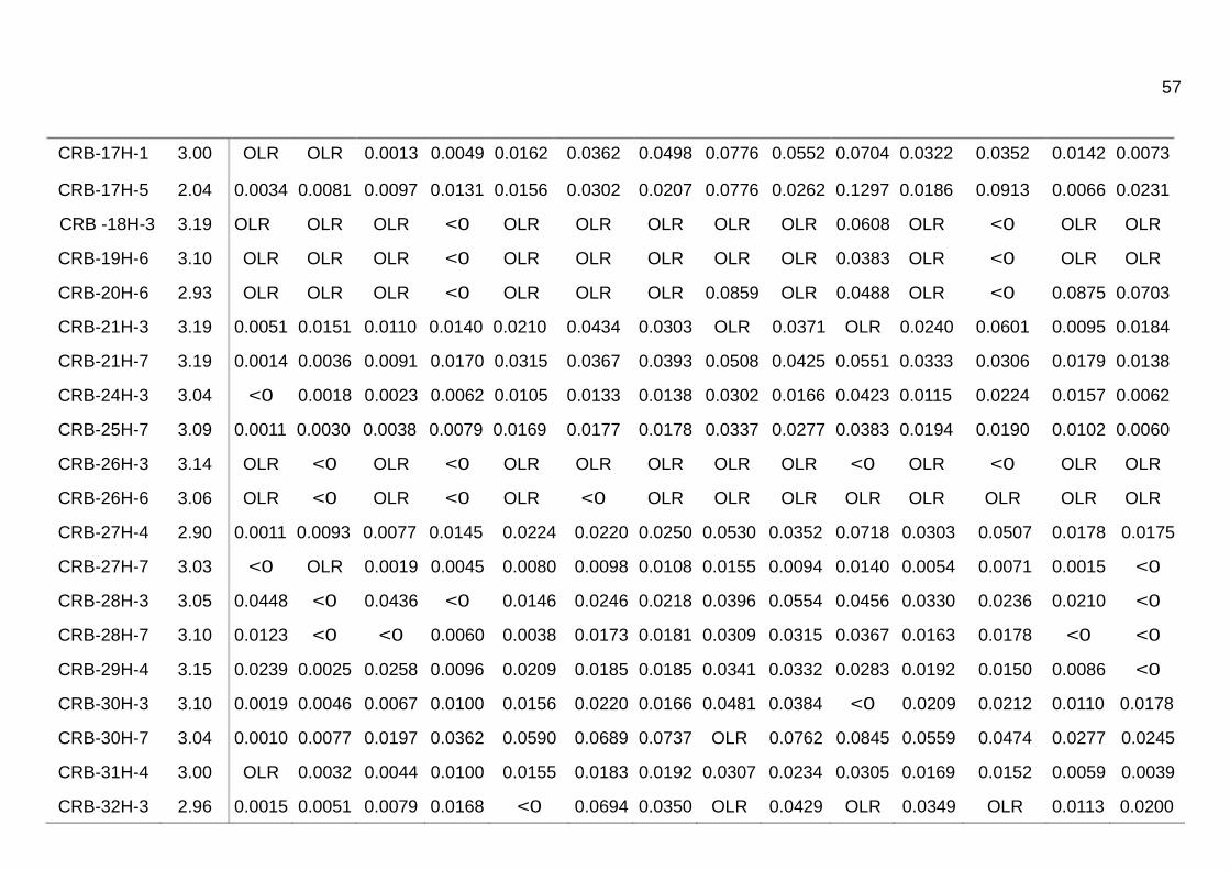
Table 3. Weight and sediment concentrations (µg g
-1) of 14 n-alkanes in the sediment samples of the cores CRA and CRB of Ceara Rise obtained by interpolation in the analytical curves.
Concentration (in µg g-1)
Weight
Sample C-22 C-23 C-24 C-25 C-26 C-27 C-28 C-29 C-30 C-31 C-32 C-33 C-34 C-35 (in g)
CRB-1H-1 2.02 <0 0.0385 0.0230 0.0415 0.0218 0.0524 0.0164 0.1119 0.0240 0.1173 0.0194 0.0575 <0 0.0159 CRB-2H-3 3.09 0.0562 0.0784 0.0581 <0 <0 0.0801 OLR OLR OLR OLR OLR 0.0792 OLR OLR CRB-3H-4 3.11 0.0111 0.0177 0.0259 0.0566 0.0752 OLR OLR OLR OLR OLR 0.0644 OLR 0.0279 0.0261 CRB-4H-3 3.13 0.0013 0.0039 0.0050 0.0115 0.0188 0.0355 0.0394 0.0708 0.0418 0.0746 0.0256 0.0376 0.0093 0.0103 CRB-6H-4 3.17 OLR <0 OLR <0 OLR <0 OLR OLR OLR OLR OLR OLR OLR OLR CRB-7H-1 3.12 0.0237 0.0161 0.0160 0.0325 0.0293 0.0330 OLR OLR 0.0257 OLR 0.0123 OLR 0.0123 0.0322 CRB-7H-3 3.20 0.0042 0.0080 0.0099 0.0196 0.0235 0.0540 0.0346 OLR 0.0424 OLR 0.0311 OLR 0.0114 0.0255 CRB-7H-5 3.07 0.0033 0.0063 0.0074 0.0166 0.0220 0.0373 0.0343 0.0830 0.0378 0.0836 0.0265 0.0530 0.0100 0.0176 CRB-8H-3 3.17 0.0024 0.0065 0.0082 0.0186 0.0208 0.0452 0.0264 0.0808 0.0296 OLR 0.0190 0.0779 0.0078 0.0193 CRB-9H-3 3.16 0.0010 0.0039 0.0039 0.0094 0.0141 0.0225 0.0196 0.0458 0.0244 0.0526 0.0169 0.0316 0.0075 0.0091
CRB-11H-3 3.02 0.0053 0.0081 0.0125 0.0209 0.0317 0.0393 0.0407 0.0691 0.0674 0.0736 0.0479 0.0429 0.0268 0.0185 CRB-11H-6 3.14 OLR OLR 0.0717 OLR OLR <0 OLR OLR OLR OLR OLR <0 OLR OLR CRB-13H-5 3.00 0.0086 0.0188 0.0232 0.0350 0.0492 0.0531 0.0568 0.0904 0.0606 0.0811 0.0479 0.0473 0.0274 0.0183 CRB-14H-3 3.06 0.0020 0.0053 0.0097 0.0174 0.0294 0.0383 0.0383 0.0611 0.0387 0.0613 0.0254 0.0324 0.0113 0.0103 CRB-15H-2 2.92 <0 <0 <0 OLR 0.0021 0.0054 0.0062 0.0113 0.0084 0.0134 0.0049 0.0066 0.0008 0.0015 CRB-16H-3 3.15 <0 OLR 0.0018 0.0049 0.0118 0.0194 0.0216 0.0440 0.0223 0.0721 0.0139 0.0345 0.0046 0.0083
57
CRB-17H-1 3.00 OLR OLR 0.0013 0.0049 0.0162 0.0362 0.0498 0.0776 0.0552 0.0704 0.0322 0.0352 0.0142 0.0073
CRB-17H-5 2.04 0.0034 0.0081 0.0097 0.0131 0.0156 0.0302 0.0207 0.0776 0.0262 0.1297 0.0186 0.0913 0.0066 0.0231 CRB -18H-3 3.19 OLR OLR OLR <0 OLR OLR OLR OLR OLR 0.0608 OLR <0 OLR OLR CRB-19H-6 3.10 OLR OLR OLR <0 OLR OLR OLR OLR OLR 0.0383 OLR <0 OLR OLR CRB-20H-6 2.93 OLR OLR OLR <0 OLR OLR OLR 0.0859 OLR 0.0488 OLR <0 0.0875 0.0703 CRB-21H-3 3.19 0.0051 0.0151 0.0110 0.0140 0.0210 0.0434 0.0303 OLR 0.0371 OLR 0.0240 0.0601 0.0095 0.0184 CRB-21H-7 3.19 0.0014 0.0036 0.0091 0.0170 0.0315 0.0367 0.0393 0.0508 0.0425 0.0551 0.0333 0.0306 0.0179 0.0138 CRB-24H-3 3.04 <0 0.0018 0.0023 0.0062 0.0105 0.0133 0.0138 0.0302 0.0166 0.0423 0.0115 0.0224 0.0157 0.0062 CRB-25H-7 3.09 0.0011 0.0030 0.0038 0.0079 0.0169 0.0177 0.0178 0.0337 0.0277 0.0383 0.0194 0.0190 0.0102 0.0060 CRB-26H-3 3.14 OLR <0 OLR <0 OLR OLR OLR OLR OLR <0 OLR <0 OLR OLR CRB-26H-6 3.06 OLR <0 OLR <0 OLR <0 OLR OLR OLR OLR OLR OLR OLR OLR CRB-27H-4 2.90 0.0011 0.0093 0.0077 0.0145 0.0224 0.0220 0.0250 0.0530 0.0352 0.0718 0.0303 0.0507 0.0178 0.0175 CRB-27H-7 3.03 <0 OLR 0.0019 0.0045 0.0080 0.0098 0.0108 0.0155 0.0094 0.0140 0.0054 0.0071 0.0015 <0 CRB-28H-3 3.05 0.0448 <0 0.0436 <0 0.0146 0.0246 0.0218 0.0396 0.0554 0.0456 0.0330 0.0236 0.0210 <0 CRB-28H-7 3.10 0.0123 <0 <0 0.0060 0.0038 0.0173 0.0181 0.0309 0.0315 0.0367 0.0163 0.0178 <0 <0 CRB-29H-4 3.15 0.0239 0.0025 0.0258 0.0096 0.0209 0.0185 0.0185 0.0341 0.0332 0.0283 0.0192 0.0150 0.0086 <0 CRB-30H-3 3.10 0.0019 0.0046 0.0067 0.0100 0.0156 0.0220 0.0166 0.0481 0.0384 <0 0.0209 0.0212 0.0110 0.0178 CRB-30H-7 3.04 0.0010 0.0077 0.0197 0.0362 0.0590 0.0689 0.0737 OLR 0.0762 0.0845 0.0559 0.0474 0.0277 0.0245 CRB-31H-4 3.00 OLR 0.0032 0.0044 0.0100 0.0155 0.0183 0.0192 0.0307 0.0234 0.0305 0.0169 0.0152 0.0059 0.0039 CRB-32H-3 2.96 0.0015 0.0051 0.0079 0.0168 <0 0.0694 0.0350 OLR 0.0429 OLR 0.0349 OLR 0.0113 0.0200

58
CRB-32H-7 3.00 OLR 0.0051 0.0113 0.0221 0.0356 0.0427 0.0451 0.0636 0.0434 0.0642 0.0327 0.0391 0.0147 0.0141
CRB-33H-7 2.07 <0 0.0176 0.0148 0.0262 0.0206 0.0275 0.0196 0.1003 0.0264 OLR 0.0221 0.1243 <0 0.0222 CRA-3R-1 3.09 OLR 0.0034 0.0044 0.0106 0.0162 0.0259 0.0269 0.0545 0.0303 0.0825 0.0235 0.0564 0.0090 0.0157 CRA-4R-1 3.12 0.0048 0.0100 0.0167 0.0343 0.0535 0.0765 0.0722 OLR 0.0707 OLR 0.0484 0.0559 0.0232 0.0216 CRA-5R-1 3.04 0.0039 0.0076 0.0085 0.0171 0.0230 0.0302 0.0285 0.0604 0.0670 0.0575 0.0444 0.0266 0.0208 0.0164 CRA-5R-4 3.05 0.0348 <0 <0 0.0229 0.0349 0.0469 0.0656 OLR 0.0693 OLR 0.0601 0.0500 0.0330 0.0246 CRA-6R-1 2.02 <0 0.0032 0.0026 0.0071 0.0140 0.0271 0.0342 0.0977 0.0519 OLR 0.0403 0.0877 0.0156 0.0197 CRA-6R-3 3.09 0.0063 0.0024 0.0029 0.0095 0.0152 0.0301 0.0391 0.0531 0.0442 0.0570 0.0328 0.0304 0.0181 0.0188 CRA-7R-3 2.00 0.0723 <0 OLR <0 0.0372 <0 0.0498 0.0784 0.0322 0.0741 0.0435 0.0401 <0 <0 CRA-8R-6 2.95 0.0051 0.0054 0.0116 0.0203 0.0402 0.0611 0.0713 OLR 0.0818 OLR 0.0572 0.0842 0.0260 0.0371 CRA-9R-4 3.09 OLR 0.0084 0.0102 0.0220 0.0542 0.0634 0.0762 OLR OLR OLR 0.0642 0.0465 0.0278 0.0193
CRA-10R-1 3.16 <0 OLR 0.0016 0.0051 0.0128 0.0198 0.0238 0.0363 0.0250 0.0343 0.0161 0.0177 0.0068 0.0057 CRA-11R-1 3.02 OLR <0 OLR <0 OLR <0 OLR 0.0671 OLR 0.0705 0.0660 0.0392 <0 <0 CRA-11R-6 3.10 0.0010 0.0040 0.0098 0.0167 0.0360 0.0588 0.0792 OLR 0.0840 OLR 0.0553 0.0509 0.0253 0.0219 CRA-12R-1 3.10 0.0111 0.0052 0.0052 0.0123 0.0234 0.0390 0.0532 0.0680 0.0551 0.0658 0.0376 0.0329 0.0162 0.0116 CRA-13R-1 3.01 <0 <0 <0 0.0173 0.0619 OLR OLR OLR OLR OLR OLR OLR 0.0576 0.0348 CRA-14R-1 3.17 0.0009 0.0029 0.0031 0.0097 0.0175 0.0338 0.0404 0.0556 0.0447 0.0494 0.0284 0.0240 0.0115 0.0076 CRA-14R-5 3.11 0.0037 0.0089 0.0132 0.0315 0.0689 OLR OLR OLR OLR OLR OLR OLR 0.0488 0,0409 CRA-15R-1 3.17 0.0301 0.0101 0.0115 0.0208 0.0318 0.0492 0.0521 OLR 0.0581 OLR 0.0503 OLR 0.0191 0,0255 CRA-16R-4 3.00 0.0311 0.0371 0.0339 <0 <0 0.0464 OLR OLR OLR 0.0707 OLR 0.0418 OLR 0,0534

59
CRA-17R-3 3.11 0.0035 0.0130 0.0148 0.0318 0.0439 0.0699 0.0801 OLR 0.0879 OLR 0.0586 OLR 0.0236 0,0263
CRA-18R-3 3.17 0.0025 0.0056 0.0062 0.0117 0.0167 0.0225 0.0190 0.0354 0.0273 0.0361 0.0291 0.0355 0.0164 0.0065 CRA-20R-1 3.32 0.0016 0.0043 0.0066 0.0147 0.0232 0.0385 0.0454 OLR 0.0496 OLR 0.0345 0.0597 0.0124 0.0133 CRA-20R-4 3.04 0.0031 0.0057 0.0086 0.0151 0.0232 0.0296 0.0335 0.0485 0.0322 0.0599 0.0241 0.0358 0.0102 0.0116 CRA-22R-3 3.04 0.0305 0.0114 0.0261 0.0245 0.0411 0.0612 0.0873 OLR OLR OLR OLR OLR OLR OLR CRA-22R-7 3.13 0.0036 0.0023 0.0042 0.0086 0.0156 0.0211 0.0230 0.0348 0.0248 0.0413 0.0171 0.0223 0.0064 0.0066 CRA-23R-3 3.18 OLR <0 OLR <0 OLR <0 OLR OLR OLR 0.0694 0.0697 <0 <0 0.0249 CRA-24R-1 3.15 0.0047 0.0131 0.0145 0.0297 0.0434 0.0753 0.0827 OLR OLR OLR 0.0778 OLR 0.0278 0.0274 CRA-26R-1 2.99 0.0018 0.0054 0.0084 0.0195 0.0427 0.0797 OLR OLR OLR OLR 0.0698 0.0551 0.0297 0.0211 CRA-26R-8 3.06 0.0026 0.0056 0.0061 0.0118 0.0205 0.0252 0.0284 0.0445 0.0379 0.0459 0.0280 0.0304 0.0131 0.0098 CRA-29R-1 2.07 0.0029 0.0033 0.0040 0.0046 0.0103 0.0222 0.0276 0.0472 0.0335 0.0427 0.0212 0.0259 0.0108 0.0076 CRA-30R-5 2.96 0.0081 0.0131 0.0081 0.0118 0.0198 OLR OLR OLR OLR OLR OLR OLR 0.0472 0.0470 CRA-32R-1 2.94 0.0924 <0 0.0904 <0 OLR <0 OLR OLR OLR OLR OLR 0.0724 0.0922 0.0878 CRA-33R-6 3.15 0.0020 0.0040 0.0053 0.0089 0.0214 0.0360 0.0443 0.0650 0.0440 0.0610 0.0290 0.0328 0.0106 0.0097 CRA-36R-7 3.14 0.0016 0.0049 0.0051 0.0102 0.0170 0.0208 0.0338 0.0416 0.0363 0.0478 0.0292 0.0273 0.0142 0.0075 CRA-39R-4 3.18 OLR <0 OLR <0 OLR OLR OLR OLR OLR OLR OLR OLR OLR OLR
OLR = Out of the linear range

60
Table 4. Concentrations (µg g
-1l) of n-alkanes in 14 samples of sediment cores CRA and CRB of Ceara Rise obtained by comparison with the area of the internal standard.
Concentration (in µg g-1)
Sample C-22 C-23 C-24 C-25 C-26 C-27 C-28 C-29 C-30 C-31 C-32 C-33 C-34 C-35
CRB-1H-1 - 0.0476 0.0298 0.0547 0.0294 0.0622 0.0231 0.1311 0.0324 0.1354 0.0256 0.069 - 0.023
CRB-2H-3 0.0564 0.0795 0.0594 - - 0.0801 0.4854 0.2746 0.4105 0.2093 0.2483 0.0805 0.1501 0.0998 CRB-3H-4 0.0123 0.0186 0.0261 0.0584 0.0733 0.0978 0.0909 0.1786 0.1017 0.1634 0.0612 0.0845 0.0279 0.027 CRB-4H-3 0.0037 0.0064 0.0075 0.0159 0.0228 0.0393 0.0449 0.0777 0.049 0.0806 0.0291 0.0423 0.012 0.0139 CRB-6H-4 0.8703 - 0.7016 - 0.5654 - 0.4506 0.2091 0.3254 0.1525 0.2207 0.1000 0.1502 0.098 CRB-7H-1 0.0233 0.0167 0.0166 0.0341 0.0294 0.0317 0.1168 0.1554 0.0268 0.1197 0.0132 0.0321 0.0132 0.0321 CRB-7H-3 0.0069 0.0111 0.0132 0.0258 0.0288 0.061 0.0412 0.1489 0.0515 0.1816 0.0361 0.1455 0.0148 0.0312 CRB-7H-5 0.0045 0.0068 0.0077 0.0165 0.02 0.0315 0.0301 0.0692 0.034 0.0687 0.0229 0.0448 0.0098 0.0166 CRB-8H-3 0.0059 0.0109 0.013 0.0285 0.0299 0.0593 0.0371 0.1058 0.0423 0.1408 0.0265 0.1021 0.0124 0.0281 CRB-9H-3 0.0034 0.0062 0.0062 0.0132 0.0173 0.0251 0.0231 0.0499 0.0288 0.0562 0.0196 0.035 0.0098 0.0124
CRB-11H-3 0.0073 0.0099 0.014 0.024 0.0332 0.0392 0.0419 0.0686 0.0702 0.0719 0.0474 0.0433 0.0278 0.0205 CRB-11H-6 0.0527 0.0766 0.0399 0.0663 0.573 - 0.5059 0.1836 0.34 0.1056 0.2371 - 0.1584 0.104 CRB-13H-5 0.0095 0.0186 0.0224 0.0352 0.046 0.048 0.0529 0.0818 0.0581 0.0726 0.0436 0.0436 0.026 0.0187 CRB-14H-3 0.0043 0.0075 0.0119 0.0214 0.0325 0.0401 0.0415 0.0638 0.0432 0.0631 0.0275 0.0347 0.0135 0.0132 CRB-15H-2 - - - 0.0114 0.015 0.0232 0.0277 0.0427 0.0348 0.0476 0.0226 0.0274 0.0092 0.0142 CRB-16H-3 0.0019 0.0025 0.0033 0.0069 0.0123 0.0181 0.0209 0.0397 0.0219 0.0631 0.0136 0.0314 0.0056 0.0096
CRB-17H-1 0.0024 0.0028 0.0033 0.0076 0.0177 0.0353 0.0496 0.0749 0.0564 0.0672 0.0318 0.035 0.0153 0.0096 CRB-17H-5 0.0057 0.0095 0.0107 0.0151 0.0161 0.0271 0.0204 0.0672 0.0256 0.1091 0.0179 0.0785 0.008 0.0227

61
CRB-18H-3 0.4820 0.0273 0.4215 - 0.3547 0.2504 0.0746 0.1978 0.0421 0.1197 - 0.0774 0.0686 0.0686 CRB-19H-6 0.0322 0.5467 - 0.4250 0.4250 0.0972 0.3801 0.1797 0.3489 0.0407 0.2287 - 0.1595 0.1018 CRB-20H-6 0.5525 0.0358 0.4716 - 0.3678 0.0911 0.2609 0.0778 0.1877 0.0443 0.1149 - 0.0790 0.0646 CRB-21H-3 0.0061 0.0145 0.011 0.0148 0.02 0.0379 0.028 0.0868 0.0348 0.0959 0.0218 0.0527 0.0097 0.0179 CRB-21H-7 0.0031 0.0049 0.0097 0.0179 0.0297 0.0331 0.0365 0.0459 0.0405 0.0489 0.0302 0.0283 0.0172 0.0144 CRB-24H-3 0.0022 0.0044 0.0049 0.0105 0.0146 0.0168 0.0183 0.0361 0.0219 0.0488 0.0151 0.0272 0.0198 0.0101 CRB-25H-7 0.0033 0.0051 0.0058 0.0111 0.0194 0.0193 0.0203 0.0357 0.0311 0.0396 0.0212 0.0209 0.0122 0.0088 CRB-26H-3 0.5859 - 0.4918 - 0.4395 0.0953 0.3141 0.0997 0.2464 - 0.1758 - 0.1092 0.0626 CRB-26H-6 0.492 - 0.7277 - 0.5864 - 0.4674 0.2169 0.3375 0.1582 0.2289 0.1037 0.1558 0.1017 CRB-27H-4 0.0038 0.0124 0.0106 0.0196 0.027 0.0255 0.0299 0.0593 0.042 0.0784 0.0345 0.0567 0.0213 0.022 CRB-27H-7 - 0.0053 0.0086 0.0164 0.0228 0.0248 0.0286 0.0378 0.0258 0.0335 0.0164 0.0194 0.0076 - CRB-28H-3 0.0565 - 0.0561 - 0.0212 0.0321 0.0301 0.0513 0.0741 0.0577 0.0425 0.0315 0.0283 - CRB-28H-7 0.015 - - 0.0096 0.0066 0.0199 0.0218 0.0347 0.0371 0.0401 0.0191 0.0208 - - CRB-29H-4 0.0295 0.0053 0.0321 0.0149 0.0271 0.0233 0.0243 0.0417 0.0427 0.0343 0.0242 0.0196 0.0122 - CRB-30H-3 0.0041 0.0067 0.0087 0.0132 0.018 0.0233 0.0189 0.0496 0.0419 - 0.0224 0.0229 0.0128 0.0203 CRB-30H-7 0.0036 0.0107 0.0236 0.0444 0.0672 0.0757 0.0833 0.0997 0.089 0.0926 0.0619 0.0536 0.0322 0.0296 CRB-31H-4 0.0028 0.0053 0.0064 0.0131 0.0177 0.0195 0.0213 0.0321 0.0261 0.0312 0.0184 0.1687 0.0078 0.0066 CRB-32H-3 0.0044 0.0084 0.0116 0.0237 - 0.0809 0.0435 0.1566 0.0543 0.2412 0.042 0.1261 0.0154 0.0263 CRB-32H-7 0.0034 0.008 0.0148 0.0287 0.0421 0.0483 0.0527 0.0721 0.0523 0.0717 0.0376 0.0452 0.0184 0.0186 CRA-3R-1 0.0027 0.0055 0.0064 0.0139 0.0187 0.0272 0.0294 0.0562 0.0337 0.083 0.0251 0.0581 0.011 0.0183

62
CRB-33H-7 - 0.0179 0.0154 0.0274 0.0211 0.0258 0.0201 0.0891 0.0266 0.1473 0.0216 0.1098 - 0.0227 CRA-4R-1 0.0034 0.006 0.0092 0.0192 0.0278 0.0382 0.0372 0.0524 0.0377 0.0536 0.0245 0.0286 0.0124 0.012 CRA-5R-1 0.0041 0.0065 0.0071 0.0139 0.017 0.0211 0.0208 0.0415 0.0481 0.039 0.0304 0.019 0.0151 0.0128 CRA-5R-4 0.0366 - - 0.0272 0.038 0.0486 0.0694 0.096 0.0755 0.0939 0.0618 0.0526 0.0353 0.0276 CRA-6R-1 - 0.0067 0.006 0.0121 0.0183 0.0305 0.0393 0.1037 0.0593 0.1558 0.0441 0.0934 0.0192 0.0246 CRA-6R-3 0.0077 0.0042 0.0046 0.0116 0.0161 0.0287 0.0381 0.0502 0.0441 0.0529 0.0313 0.0295 0.0183 0.0196 CRA-7R-3 0.064 - 0.5365 - 0.0357 - 0.0467 0.0706 0.0321 0.0659 0.0399 0.0373 - - CRA-8R-6 0.0062 0.0064 0.0116 0.0205 0.0363 0.0524 0.0628 0.1135 0.0741 0.1348 0.0492 0.0728 0.0236 0.0336 CRA-9R-4 0.0025 0.0086 0.01 0.0213 0.0467 0.0527 0.0649 0.0818 0.0784 0.0766 0.0533 0.0397 0.0243 0.018 CRA-10R-1 0.0019 0.0035 0.0049 0.0109 0.0205 0.0285 0.0353 0.0512 0.0379 0.0477 0.024 0.0262 0.0117 0.0113 CRA-11R-1 0.2210 - 0.1979 - 0.1601 - 0.112 0.0743 0.1197 0.0768 0.0718 0.0443 0.0018 - CRA-11R-6 0.003 0.0058 0.0113 0.0193 0.0367 0.0567 0.078 0.1065 0.0854 0.095 0.0534 0.0502 0.0258 0.0233 CRA-12R-1 0.0126 0.0071 0.007 0.0153 0.0251 0.039 0.0543 0.0677 0.058 0.0647 0.0377 0.0337 0.0176 0.0139 CRA-13R-1 - - - 0.0205 0.0628 0.169 0.2448 0.305 0.2389 0.2146 0.1355 0.1016 0.0575 0.0364 CRA-14R-1 0.0029 0.0047 0.0049 0.0121 0.0189 0.033 0.0406 0.0541 0.046 0.0475 0.0282 0.0244 0.0126 0.0097 CRA-14R-5 0.0051 0.0097 0.0134 0.0316 0.0633 0.1121 0.1554 0.2227 0.1604 0.2031 0.0992 0.1045 0.0446 0.0383 CRA-15R-1 0.027 0.0104 0.0116 0.0211 0.0295 0.0431 0.0471 0.1223 0.054 0.1965 0.0441 0.1153 0.018 0.0241 CRA-16R-4 0.0289 0.0347 0.0319 - - 0.0422 0.2055 0.103 0.1906 0.0636 0.1003 0.0388 0.0846 0.0497 CRA-17R-3 0.0046 0.0123 0.0138 0.0296 0.0381 0.0578 0.068 0.1144 0.0769 0.1284 0.0486 0.0733 0.0208 0.0237 CRA-18R-3 0.0047 0.0077 0.0083 0.0152 0.0194 0.0243 0.0217 0.0378 0.031 0.0378 0.031 0.0379 0.0185 0.0093

63
CRA-20R-1 0.0048 0.0084 0.0113 0.024 0.034 0.0526 0.0637 0.119 0.0714 0.1514 0.0476 0.0816 0.0189 0.021 CRA-20R-4 0.0054 0.0079 0.0109 0.019 0.0262 0.0315 0.0368 0.0513 0.0364 0.0618 0.0262 0.0383 0.0124 0.0147 CRA-22R-3 0.0209 0.0088 0.0184 0.0187 0.0287 0.0406 0.0592 0.0788 0.0749 0.0944 0.0711 0.0787 0.0643 0.0706 CRA-22R-7 0.0055 0.0042 0.006 0.0114 0.0174 0.0217 0.0246 0.0354 0.027 0.0409 0.0182 0.0233 0.0081 0.009 CRA-23R-3 0.2052 - 0.1937 - 0.1303 - 0.1094 0.0893 0.0461 0.0614 0.0614 - - 0.0241 CRA-24R-1 0.0059 0.0132 0.0143 0.0295 0.04 0.066 0.0745 0.1553 0.0889 0.2064 0.068 0.1176 0.0258 0.0261 CRA-26R-1 0.0035 0.0065 0.009 0.0201 0.0391 0.0692 0.0968 0.1248 0.1042 0.101 0.0608 0.0492 0.0272 0.0205 CRA-26R-8 0.0047 0.0075 0.0079 0.0147 0.0223 0.0258 0.0299 0.0448 0.0403 0.0454 0.0285 0.0312 0.0145 0.0121 CRA-29R-1 0.0058 0.0061 0.0066 0.0084 0.0131 0.0231 0.0294 0.0471 0.0358 0.042 0.0226 0.027 0.0129 0.011 CRA-30R-5 0.0047 0.007 0.0047 0.007 0.0102 0.0201 0.034 0.1454 0.0733 0.1997 0.0528 0.096 0.0224 0.0227 CRA-32R-1 0.0826 0.071 0.0826 - 0.0976 - 0.091 0.2326 0.0977 0.1558 0.1992 0.0668 0.0842 0.081 CRA-33R-6 0.0037 0.0053 0.0064 0.0106 0.021 0.0326 0.0411 0.0585 0.0421 0.0543 0.0267 0.0303 0.011 0.0109 CRA-36R-7 0.0038 0.0071 0.0072 0.0136 0.0196 0.0225 0.0366 0.0438 0.0403 0.0493 0.0309 0.0294 0.0162 0.0103 CRA-39R-4 0.4394 - 0.4148 - 0.349 0.0736 0.2584 0.1881 0.207 0.2252 0.1311 0.1094 0.0684 0.0658
-: Species not detected.

64
The values for concentrations calculated using external analytical
curves ranged from 0.0009 to 0.1297 µg g-1. Concentrations calculated from the
area compared to standard squalene ranged from 0.0019 to 0.8703 µg g-1.
Since the samples had a range of very high concentration of n-alkanes,
it was not possible to quantify some analytes. Quantification by the internal standard method have no limitation of the linear range, making it possible to quantify analytes in a wider range of concentrations.
4.4. QUALITATIVE DETERMINATION OF ALKENONES
The alkenones were identified qualitatively by injection of samples in a
gas chromatograph coupled to a mass spectrometry detector, performed at the Laboratory NIOZ, Netherlands. The typical chromatogram with identified peaks is shown in Figure 28.
Figure 21. Representative chromatogram of sediment sample containing alkenones.

65
The chromatograms obtained for the alkenone fractions of the samples
are in the Appendix D.
4.5. QUANTITATIVE DETERMINATION OF ALKENONES
As there are no standard available for construction of the analytical
curve, the alkenones were quantified by comparing the peak area of the internal
standard and the area of the analyte. The average concentrations in µg g-1, for
the samples are shown in Table 15.
Table 15. Concentrations (µg g-1) of alkenones in sediment samples of cores CRA and CRB of
Ceara Rise obtained by comparison with the area of the internal standard.
Concentration (in µg g-1)
Sample Name C37:3 C37:2 C38EK C38MK C39
925B-2H-3-(45-48) 0.006 0.108 0.071 0.036 0.011
925B-2H-6-(92-95) 0.020 0.331 0.232 0.102 0.041
925B-3H-4-(114-117) 0.017 0.301 0.155 0.071 0.011 925B-4H-3-(100-103) 0.001 0.050 0.029 0.014 0.002
925B-5H-3-(43-46) 0.003 0.094 0.043 0.025 0.006 925B-5H-6-(25-28) 0.008 0.192 0.093 0.047 0.012 925B-6H-4-(58-61) 0.005 0.151 0.082 0.048 0.013 925B-7H-1-(15-19) - 0.132 0.084 0.040 0.015 925B-7H-3-(53-56) 0.015 0.386 0.130 0.112 0.035 925B-7H-5-(40-43) 0.001 0.102 0.057 0.026 0.004 925B-8H-3-(86-89) 0.015 0.239 0.140 0.069 0.022 925B-9H-3-(86-89) 0.001 0.084 0.043 0.019 0.005
925B-10H-3-(86-89) 0.006 0.152 0.081 0.036 0.011

66
925B-11H-3-(87-90) - 0.033 0.018 0.006 0.001
925B-11H-6-(43-48) 0.007 0.205 0.116 0.040 0.015 925B-12H-4-(86-89) 0.002 0.064 0.036 0.017 0.004 925B-13H-5-(25-28) - - - - -
925B-14H-3-(100-103) - 0.032 0.016 0.006 - 925B-15H-2-(30-33) - 0.032 0.019 0.012 -
925B-16H-3-(5-8) - 0.032 0.016 0.004 -
925B-17H-1-(104-107) - 0.020 0.013 0.007 - 925B-17H-5-(10-14) - 0.021 0.016 0.004 -
925B-18H-3-(122-125) - 0.006 0.006 - - 925B-19H-3-(87-90) - - - - - 925B-19H-6-(28-31) 0.004 0.044 0.032 0.012 0.005 925B-20H-6-(60-63) - 0.017 - - - 925B-21H-3-(19-23) - 0.009 0.009 0.004 - 925B-21H-7-(44-47) - 0.008 0.008 0.001 - 925B-22H-7-(43-46) 0.004 0.022 0.017 0.012 0.021 925B-23H-5-(42-45) - 0.017 0.011 0.005 0.001
925B-24H-3-(122-125) - 0.008 0.006 0.003 - 925B-25H-2-(25-28) - 0.007 0.005 - - 925B-25H-7-(43-47) - - - - - 925B-26H-3-(91-94) - - - - -
925B-26H-6-(104-107) - - - - - 925B-27H-4-(46-50) - - - - - 925B-27H-7-(29-32) - 0.002 0.001 - - 925B-28H-3-(59-62) - 0.006 0.006 0.005 - 925B-28H-7-(68-71) - - - - - 925B-29H-4-(44-47) - 0.013 0.009 0.003 - 925B-30H-3-(77-80) - 0.030 0.018 0.007 0.001

67
925B-30H-7-(43-46) 0.001 0.057 0.015 0.012 0.002
925B-31H-4-(119-122) 0.003 0.109 0.058 0.021 0.006 925B-32H-3-(50-53) 0.004 0.140 0.081 0.019 0.009 925B-32H-7-(10-13) 0.002 0.026 0.014 0.015 - 925B-33H-7-(10-15) - 0.043 0.065 0.010 0.008 925A-3R-1-(95-98) 0.002 0.117 0.076 0.024 0.006 925A-4R-1-(58-61) - 0.013 0.008 0.003 - 925A-5R-1-(52-55) - 0.014 0.008 0.001 - 925A-5R-4-(52-55) - 0.014 0.011 0.037 - 925A-6R-1-(62-65) 0.008 0.516 0.307 0.055 0.029
925A-6R-3-(111-114) 0.003 0.017 0.010 0.002 -
925A-7R-3-(6-10) - 0.010 0.007 0.008 -
925A-8R-2-(136-139) - 0.030 0.018 0.009 0.002
925A-8R-6-(80-83) 0.002 0.093 0.056 0.011 0.005
925A-9R-4-(131-134) - - - - - 925A-10R-1-(128-131) - - - - - 925A-11R-1-(41-44) - - - - - 925A-11R-6-(22-25) - - - - - 925A-12R-1-(23-26) 0.003 0.042 0.021 0.007 - 925A-13R-1-(48-51) - 0.017 0.007 0.004 -
925A-14R-1-(6-9) - 0.008 0.005 0.002 -
925A-14R-5-(125-128) 0.002 0.053 0.029 0.012 0.003 925A-15R-1-(97-100) 0.006 0.235 0.142 0.058 0.017 925A-15R-7-(20-23) 0.003 0.061 0.031 0.011 0.003 925A-16R-4-(67-70) 0.004 0.334 0.184 0.069 0.019
925A-17R-3-(137-140) 0.004 0.234 0.151 0.057 0.018
925A-18R-3-(8-11) 0.002 0.093 0.054 0.020 0.006
925A-18R-7-(16-19) 0.006 0.237 0.134 0.074 0.021

68
925A-19R-3-(106-109) 0.014 0.174 0.108 0.038 0.012
925A-20R-1-(55-58) 0.001 0.062 0.041 0.014 0.006 925A-20R-4-(66-69) 0.017 0.033 0.025 0.009 0.004 925A-22R-3-(26-29) 0.002 0.091 0.053 0.021 0.004 925A-22R-7-(26-29) 0.004 0.018 0.011 0.004 -
925A-23R-3-(136-139) - 0.050 0.035 0.012 0.006 925A-24R-1-(74-77) 0.015 0.156 0.112 0.044 0.017 925A-26R-1-(13-16) - 0.021 0.016 0.006 0.001
925A-26R-8-(6-9) - 0.040 0.033 0.033 0.005
925A-29R-1-(42-45) - 0.094 0.073 0.022 0.011 925A-30R-5-(15-18) 0.001 0.059 0.045 0.014 0.006 925A-32R-1-(38-41) - 0.060 0.046 0.014 0.003 925A-33R-6-(42-45) - 0.048 0.039 0.011 0.003 925A-36R-7-(46-49) - 0.037 0.031 0.009 0.005 925A-39R-4-(81-84) 0.001 0.154 0.128 0.047 0.020
-: Species not detected.
Values for concentrations calculated from the area compared with the
2-nonadecanone standard ranged from 0.001 to 0.516 µg g-1
. Except for
samples CRB 33 H-7 and CRA 5 R-4, C37:2 has the highest concentration
among the other alkenones detected.
The predominant concentration of C37:2 was also found by Boot et al.
(2006) when evaluating the concentration of alkenones at site 942 (5°45'N,
49°6'W), located in the Amazon Fan. The dominance of C37:2 alkenones in
relation to the other suggests that their source is predominantly seaweed (ZINK
et al., 2001).
However, caution is needed with proxies results obtained from the
quantification of lipids because of its degradation. As C37: 2 suffer less the effect

69
of degradation that C37: 3, the relative ratio between the compounds may be
affected, resulting in a bias in the calculated temperatures (HOEFS et al., 2002).
4.6. PROXIES CARBON PREFERENCE INDEX AND AVERAGE
CHAIN LENGTH
CPI values, which are calculated according to Equation 4, varied over
the years and record, as can be seen in Figure 29. The minimum values are between 0.18 and 0.19 and are found in the portion of the core corresponding to the beginning of the Late Miocene. The maximum value is 4.1, corresponding to the end of the Middle Miocene.
In the intervals in which CPI values varies between ~1 and ~4, it is
possible to suggest that the primary source of n-alkane was wax leaves of terrestrial plants (DUAN et al., 2010). At low degree, there is the influence of the activity of marine microorganisms as a source of aliphatic hydrocarbons the CPI values are less than 1(JENG et al., 2006; DUAN et al., 2010).
According to the proxy CPI, the main source of organic materials
present in the studied cores comes from terrestrial source. This result is in agreement with the study by Boot et al. (2006) in the assessment of organic materials input to Amazon Fan, in which all sediments originating from site 942, were evaluated according to the CPI and indicated that the main source of organic matter of the area comes from terrigenous material.

CPI
70
CPI
4,5
4
3,5
3
2,5
2
1,5
1
0,5
0 30 25 20 15 10 5 0
Age (ma)
Figure 22. Calculated CPI values along the record at sites 925 A and 925 B, situated at Ceara
Rise.
Throughout the record, the value of ACL varies between ~26.6 and
~30.7 (Figure 30), suggesting that the main source of n-alkanes also is derived from terrestrial sources, and meaning, in most cases, that the organic material was transported from the land to the sea due to the action of winds and the flow of rivers.
Boot et al. (2006) also evaluated the results of the ACL on site 942. In
this work, the calculated values of ACL did not varied much, lying around ~29.8. This fact led researchers to conclude that small variations in ACL indicate consistency in the source of vegetation type, in which the primary source was also terrigenous.

ACL
71
ACL
31 30,5
30 29,5
29 28,5
28 27,5
27 26,5
26 30 25 20 15 10 5 0
Age (m.a)
Figure 30. ACL values calculated over the record sites 925 A and 925 B,
situated at Ceara Rise.
Dobson et al. (2001) also evaluated the terrigenous sediment on Ceara
Rise and concluded that most of the terrigenous sediment deposited on Ceara Rise is product of weathering of rocks in the Andes, because terrigenous materials derived from other sources are hardly deposited in Ceara Rise due its location and the intense amount of sediment produced in Amazon, that forms a physical barrier.
In general, the concentration of n-alkanes is higher than alkenones
because these are best preserved. This happens because the n-alkanes are tougher and its headquarters act as a protective barrier, which is why terrigenous lipids are better preserved than those present in marine sediments (HOEFS et al., 2002).
4.7. RECONSTRUCTION OF SST

72
The temperature profile obtained from the calculation of (Equation
1) for samples in which it was possible to quantify C37:2 and C37:3 is shown in
Figure 31.
Figure 31. Alkenone derived sea surface temperature (°C) record at sites 925 A (represented in
red) and 925 B (in blue), situated at Ceara Rise.
According to Figure 31, it can be observed that between Pleistocene
and the Middle Pliocene there was little variation in the SST. From the Middle Pliocene to half of Late Miocene the tendency of the SST was reach coldest values, followed by heating until the beginning of the Early Miocene. At the end

73
of Early Miocene there was the lowest recorded SST (22.5 °C), which was followed again by a heating tendency until the registration of the highest temperature (28.5 °C) at half the Early Oligocene.
The work of Boot et al. (2006) were unable to estimate the SST for
various samples of site 942. In this work, which included samples from 35 kyr, the estimated SST ranged from 23 to 26 °C in the glacial period, corresponding to the end of Pleistocene, and C37:3 was not detected in the glacial periods.
During the same period, the SST estimated for samples of Ceara Rise used in
this work was ~26 °C.
Temperatures estimated in Ceara Rise are consistent with the global
trend already observed by other researchers. Pearson et al. (2007) stated that the global trend during the Early Oligocene, period in which the planet was characterized as 'Greenhouse World' was heating. In samples analyzed in this work, the Early Oligocene was the period in which the highest SST was estimated (~ 28 °C).
In the studied cores, there was no sample covering the Late Oligocene,
but estimates of SST from the beginning of the Early Miocene suggest that the trend was cooling, fact that is consistent with prediction made by Pearson et al. (2007) and coincides with the onset of glaciers.
During the Miocene until to the Early Pliocene, the world's propensity to
cooling, but with intervals of higher temperatures, already observed by FEARY et al. (1990), ZACHOS et al. (2001) and LISIECKI et al. (2007). It was also observed in cores analyzed in this work. The interval when the highest temperatures were estimated happened in Middle Miocene. This period also coincides with the last interval of warmer temperatures than today. SSTs estimated in the Rio Grande Rise for this period are even 3 °C higher than the temperatures recorded today (DOWSETT et al., 1996).

74
Studies by Haywood et al. (2009) estimated an overall increase of SST
from the Early Pliocene to the present day, which can also be observed for samples from site 925 at Ceara Rise (Figure 32).
The results obtained in the estimative of SST in Ceara Rise are
consistent with other studies conducted, even when using different extraction methods or tool proxies. Therefore, this study may contribute to understanding global trends of variation of SST over the last 30 Ma.

75
5. CONCLUSIONS
The method for extraction of n-alkanes and alkenones in sediment
samples, first used in AQQUA Group, generated satisfactory results in agreement with other studies conducted in what concerns the reconstruction of sea surface temperatures and main origin of organic materials present in these sediments.
The extraction with ultrasonic used little volume of solvent, resulted in
small amount of residues and generated satisfactory results in relation to the recovery test of n-alkanes. For the recovery of alkenones the recovery factors were not so good due the presence of UCM in chromatograms and absence of alkenones used in this study at the sediment used for the recovery test.
Quantification of n-alkanes was performed from analytical curves and
the concentrations obtained from the curves were compared with the measurement performed by the comparison of the area of the analyte to the area of standard added to the sample, quantification method commonly used in studies of paleotemperature. The results were concordant for both quantifying and statistically equal, which, by analogy, justified the quantification of alkenones only by the method of comparing areas, since there is no standard of alkenones commercially available.
The Carbon Preference Index and Average Chain Length proxies used
to determine the main source of the organic material present in sediments were both consistent and showed that the main source of organic matter in sediments of the Ceara Rise is coming from terrigenous source, that is, the material present in the coastal region was sent to the place from transport of rivers and winds.
The concentration of the alkenones ranged from 0.001 to 0.516 µg g-1
and C37:2 was the compound with the highest concentration among these

76
alkenones. The proxy brought estimated values of SST ranging between
22.5 and 28.5 °C. The results presented are in agreement with other studies that
show the South Atlantic paleoclimatic reconstruction.
Despite the temporal distance of the estimated temperature records, it
was possible to show the general trend of warming/cooling that occurred in Ceara Rise during the last 30 Ma, result that contributes to a better understanding of variations in temperature that occurred across the South Atlantic and collaborates with studies of others important world regions, as the Amazon Fan.

77
6.BIBLIOGRAPHIC REFERENCE
ANVISA, Resolução-RE n° 899 – Guia de validação de métodos analíticos e bioanalíticos, de 29 de maio de 2003. Available at <http://portal.anvisa.gov.br/wps/wcm/connect/4983b0004745975da005f43fbc4 c6735/RE_899_2003_Determina+a+publica%C3%A7%C3%A3o+do+Guia+pa ra+valida%C3%A7%C3%A3o+de+m%C3%A9todos+anal%C3%ADticos+e+bi oanal%C3%ADticos.pdf?MOD=AJP> Accessed July 29,2014.
Aragão N. M.; Quim. Nova, 2009, 32, 2476.
Blyth A. J.; Baker A.; Collins M. J.; Penkman E. H.; Gilmour M. A.; Moss J. S.; Genty D.; Drysdale R. N.; Quat. Sci. Rev., 2008, 27, 905.
Boot C. S.; Ettwein V. J.; Maslin M. A.; Weyhenmeyer C.E.; Pancost R.D.; Org. Geochem. 2006, 37, 208.
Brassel S. C.; Eglinton G.; Marlowe I. T.; Pflaumann U.; Sarnthein M.; Nature,1986, 320, 129.
Castañeda I. S.; Schouten S.; Quat. Sci. Rev., 2008, 30, 2851.
Curry W. B.; Shackleton N. J.; Richter C.; Sci Results, 1995, 154,1.
Dobson D. M.; Dickens G. R.; Rea D. K.; Sci Results, 1997, 154, 465.
Dobson D. M.; Dickens G.; Palaegeogr. Palaeclimatol. Palaeoclimatol., 2001, 165, 215.
Duan F.; He K.; Liu X.; J. Environ. Sci., 2010, 22, 998.
Eglinton T. I.; Eglinton G.; Earth Planet. Sci. Lett., 2008, 275,1.
78
Eigenbrod F.; Armsworth P. R.; Anderson B. J.; Heinemeyer A.; Gillings S.; Roy D. R.; Thomas C. D.; Gaston K. J. J.; Appl. Ecol., 2010, 47, 377.
Feary D. A.; Davies P. J.; Pigram C. J.; Symonds P. A.; Palaegeogr. Palaeclimatol. Palaeoclimatol., 1991, 89, 341.
Figueiredo J.; Hoorn C.; Ven P.; Soares E.; Geological Society of America, 2009, 37, 619.
Flood R. D.; Piper D. J. W.; Sci Results, 1997, 155, 653.
Friztsons E.; Mantovan L. E.; Aguiar A. V.; Rev. Est. Amb., 2008, 10,49.
Haywood A. M. M.; Dowsett H. J., Valdes P. J., Lunt D. J., Francis J. E.; Sellwood B. W.; Phil. Trans. R. Soc. A, 2009, 367, 3.
Hebert T. D.; Treatise on Geochemistry, 2003, 6, 391.
Helmond N. A. G. M. Palynological and organic geochemical characterization of marine and terrestrial Early Pleistocene climate in
northwest Europe. 2010. Dissertation (Master in Biogeology) – Utrecht
University, Netherlands, 2010.
Heinrich S.; Zonnevel K. A. F.; Palaegeogr. Palaeoclimatol. Palaeclimatol., 2013, 386, 599.
Hoefs M. J. L.;Rupstrra W. I.C.; Damsté J. S. S.; Geochim. Cosmochim. Ac., 2002, 66, 2719.
Jeng W.; Mar. Chem., 2006, 102, 242.
Kim J. H.; Huguet C.; Zonneveld K. A. F.; Versteegh G. J. M.; Roeder W.; Damsté J. S. S.; Schouten S.; Geochim. Cosmochim. Ac., 2009, 73, 2888.
Kumar N.; Embley R. W.; Geological Society of America Bolletin, 1977, 88, 683.

79
Lisiecki L. E.; Raymo M. E.; Quartenary Sci. Reviews, 2007, 26, 56.
Mann M. E.; Zhang Z.; Hughes M. K.; Bradley R.S.; Miller S. K.; Rutherford S.; Ni F. P.; Natl. Acad. Sci. USA, 2008, 105, 13252.
Meyers P. A.; Org. Geochem., 2003, 34, 261.
Miller J. M.; Miller J. C.; Statistics and Chemometrics for Analytical Chemistry, 5° ed.; Pearson Education Limited: England, 2005
Müller P.; Kirst G.; Ruhland G.; Storch I.; Rosell-Melé A.; Geochim. Cosmochim. Acta, 1998, 62, 1757-1772.
Murayama M.; Nagai H.; Imamura M.; Hatori S.; Kobayashi K.; Taira A.; Nucl. Instr. and Meth. In Phys. Res. B, 1997, 123, 302.
http://www.cpc.ncep.noaa.gov/data/indices/sstoi.atl.indices, accessed in
November of 2014.
Ohkouchi N.; Wada E.; Sci Results, 1997, 154, 501.
Pearson P. N.; Dongen B. E.; Nicholas C. J.; Pancost R. D.; Schouten S.; Singano J. M.; Wade B. S.; Geology, 2007, 35, 211.
Peter B.; Earth Planet. Sci. Lett., 2004, 220, 3.
Prahl F .G.; Wakeham S. G.; Nature, 1987, 330, 367.
Prahl F. G.; Mix A. C.; Sparrow M. A.; Geochim. Cosmochim. Ac., 2006, 70, 101.
Ribani M.; Bottoli C. B. G.; Collins C.H.; Jardim I. C. S. F.; Melo L. F. C.; .; Quím. Nova, 2004, 27, 771.
Riberio F. A. L.; Ferreira M. M. C; Morano S. C.; Silva L. R.; Schneider R. P.; Quím. Nova, 2008, 31, 164.

80
Rommerskirchen F.; Condon T.; Mollenhauer G.; Dupont L.; Schefuss E.; Paleoceanography, 2011, 26, 1.
Sachs J. P.; Pahnke K.; Smittenberg R.; Zhang Z.; Encyclop. Quat. Sci., 2013, 2, 775.
Smith M.; Deckker P.; Rogers J.; Brocks J.; Hope J.; Schmidt S.; Santos R. L.; Shouten S.; Org. Geochem., 2013, 64, 94.
Spera A. M. Registro de variações ambientais dos últimos 3000 anos da
Região da Ria do Mamanguá, Rio de Janeiro, utilizando marcadores
orgânicos moleculares. 2012. Dissertation (Master in Science) –
Oceanographic Institute, University of Sao Paulo, Sao Paulo, 2012.
Toney J. L.; Theroux S.; Andersen R. A.; Coleman A.; Amaral-Zettler L.; Huang
Y.; Geochim. Cosmochim. Ac., 2012, 78, 51.
Villalba R.; Grosjean M.; Kiefer T.; Palaeogeogr. Palaecocl.,2009, 281,175.
Zachos J.; Pagani M.; Sloan L.; Thomas E.; Billups K.; Sci., 2001, 292, 686.
Zachos J. C.; Dickens G. R.; Zeebe R. E.; Nature, 2008, 451, 279.
Zink K. G..; Leythaeuser D.; Melkonian M.; Schwark L.; Geochim. Cosmochim. Ac, 2001, 65, 253.

81
APPENDIX
APPENDIX A: GEOLOGICAL TIME SCALE

82
APPENDIX B. RESULTS OF THE WORK OF CURRY ET AL. (1995)

83

84

85

86

87
APPENDIX C. CHORMATOGRAMS OF N-ALKANES’ EXTRACTS
Sample CRA 3 R1 Sample CRA 5 R4
Sample CRA 4 R1 Sample CRA 6 R1
Sample CRA 5 R1 Sample CRA 6 R3

88
Sample CRA 7 R3 Sample CRA 10 R1
Sample CRA 8 R6 Sample CRA 11 R1
Sample CRA 9 R4 Sample CRA 11 R6

89
Sample CRA 12 R1 Sample CRA 14 R5
Sample CRA 13 R1 Sample CRA 15 R1
Sample CRA 14 R1 Sample CRA 16 R4

90
Sample CRA 17 R3 Sample CRA 20 R4
Sample CRA 18 R3 Sample CRA 22 R3
Sample CRA 20 R1 Sample CRA 22 R7

91
Sample CRA 23 R3 Sample RA 26 R8
Sample CRA24 R1 Sample CRA 29 R1
Sample CRA 26 R1 Sample CRA 30 R5

92
Sample CRA 32 R1 Sample CRA 39 R4
Sample CRA 33 R6 Sample CRB1 H1
Sample CRA 36 R7 Sample CRB 2 H3

93
Sample CRB 3 H4 Sample CRB 7 H1
Sample CRB 4 H3 Sample CRB 7 H3
Sample CRB 6 H4 Sample CRB 7 H5

94
Sample CRB 8 H3 Sample CRB 11 H6
Sample CRB 9 H6 Sample CRB 13 H5
Sample CRB 11 H3 Sample CRB 14 H3

95
Sample CRB 15 H2 Sample CRB 18 H3
Sample CRB 16 H3 Sample CRB 19 H3
Sample CRB 17 H5 Sample CRB 20 H6

96
Sample CRB 21 H3 Sample CRB 25 H7
Sample CRB 21 H7 Sample CRB 26 H3
Sample CRB 24 H3 Sample CRB 26 H6

97
Sample CRB 27 H4 Sample CRB 28 H7
Sample CRB 27 H7 Sample CRB 29 H4
Sample CRB 28 H3 Sample CRB 30 H3

98
Sample CRB 30 H7 Sample CRB 32 H7
Sample CRB 31 H4 Sample CRB 33 H7
Sample CRB 32 H3

99
APPENDIX D. CHORMATOGRAMS OF ALKENONES’ EXTRACTS
Sample CRA 3 R1 Sample CRA 6 R1
Sample CRA 4 R1 Sample CRA 6 R3
Sample CRA 8 R2
Sample CRA 5 R1

100
Sample CRA 8 R6 Sample CRA 11 R1
Sample CRA 9 R4 Sample CRA 12 R1
Sample CRA 10 R1 Sample CRA 13 R1
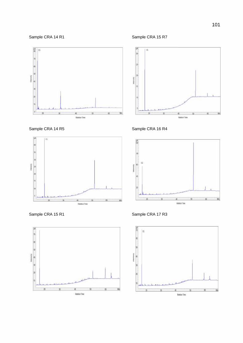
101
Sample CRA 14 R1 Sample CRA 15 R7
Sample CRA 14 R5 Sample CRA 16 R4
Sample CRA 15 R1 Sample CRA 17 R3

102
Sample CRA 18 R3 Sample CRA 20 R1
Sample CRA 18 R7 Sample CRA 20 R4
Sample CRA 19 R3 Sample CRA 22 R3

103
Sample CRA 22 R7 Sample CRA 26 R1
Sample CRA 23 R3 Sample CRA 26 R8
Sample CRA 24 R1 Sample CRA 29 R1

104
Sample CRA 30 R5 Sample CRA 36 R7
Sample CRA 32 R1 Sample CRA 39 R4
Sample CRA 33 R6 Sample CRB 2 H3

105
Sample CRB 2 R6 Sample CRB 5 H3
Sample CRB 3 H4 Sample CRB 5H6
Sample CRB 4H3 Sample CRB 6H4

106
Sample CRB 7H1 Sample CRB 8H3
Sample CRB 7H3 Sample CRB 9H3
Sample CRB 7H5 Sample CRB 10H3

107
Sample CRB 11 H3 Sample CRB 13H5
Sample CRB 11H6 Sample CRB 14 H3
Sample CRB 12 H4 Sample CRB 15 H2

108
Sample CRB 16 H3 Sample CRB 18 H3
Sample CRB 17 H1 Sample CRB 19 H3
Sample CRB 17 H5 Sample CRB 19 H6

109
Sample CRB20 H6 Sample CRB 22 H7
Sample CRB 21 H3 Sample CRB 23 H5
Sample CRB 21 H7 Sample CRB 24 H3
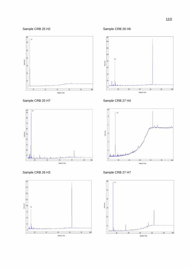
110
Sample CRB 25 H2 Sample CRB 26 H6
Sample CRB 25 H7 Sample CRB 27 H4
Sample CRB 26 H3 Sample CRB 27 H7

111
Sample CRB 28 H3 Sample CRB 30 H3
Sample CRB 28 H7 Sample CRB 30 H7
Sample CRB 29 H4 Sample CRB 31 H4

112
Sample CRB 32 H3
Sample CRB 32 H7
Sample CRB 33 H7

113