UNIVERSITY OF CALIFORNIA Economics 134 DEPARTMENT OF ECONOMICS Spring 2018

Professor David Romer

LECTURE 6

DOES MONETARY POLICY MATTER? FEBRUARY 5, 2018

I. MONEY-OUTPUT REGRESSIONS A. The issue: determining the effects of monetary changes B. A simple model of the determination of GDP growth 1. The model 2. An aside on percent changes and changes in logs C. Estimating the parameters of the model using an OLS regression D. The results of a typical money-output regression 1. Specification 2. Results 3. Interpreting the results if we believed was not omitted variable bias E. Possible sources of omitted variable bias II. FRIEDMAN AND SCHWARTZ A. Friedman and Schwartz’s approach B. The key episodes C. A simple version of Friedman and Schwartz’s model D. Friedman and Schwartz’s results E. Discussion and assessment III. ROMER AND ROMER A. The specific type of episode Romer and Romer focus on B. Identifying the episodes C. A simple version of Romer and Romer’s model D. Regression results 1. The equation that Romer and Romer actually estimate 2. Results E. Discussion and assessment F. Romer and Romer on Friedman and Schwartz (time permitting)

LECTURE 6 Does Monetary Policy Matter?

February 5, 2018

Economics 134 David Romer Spring 2018

Announcement

• Problem Set 1 is due at the beginning of lecture next time (Feb. 7).

• Optional problem set work session: Today (Monday, Feb. 5), 6:45–8:15, in 597 Evans Hall.

I. MONEY-OUTPUT REGRESSIONS

The Issue

• We would like to know if monetary changes have important macroeconomic effects (for example, on real GDP and unemployment).

A Simple Model of GDP Growth

∆ ln Yt = a + b ∆ ln Mt + et, where: - Y is real GDP; - M is the money stock; - et reflects all other factors affecting growth; - a and b are parameters; - ∆ denotes change; - ln denotes natural log.

Aside: Growth Rates and Changes in Logs • Useful fact: When the percent change in a

variable is small, the change in its natural log is approximately 0.01 times its percent change. – For example: If x rises by 1%, the change in

ln x is ln 1.01, which is 0.00995. – Another example: If x rises by 10%, the

change in ln x is ln 1.1, which is 0.0953. • Partly for that reason, economists often use

the change in the natural log of a variable rather than its percent change.

Estimating the Parameters of the Model Using an OLS Regression

∆ ln Yt = a + b ∆ ln Mt + et.

Choose a and b to fit the data as well as possible (that is, so a + b ∆ ln Mt is on average as close as possible to ∆ ln Yt).

The Specification of a Typical Money–Output Regression

• Regression equation: ∆ ln Yt = a + b0 ∆ ln Mt + b1 ∆ ln Mt-1 + b2 ∆ ln Mt-2 + b3 ∆ ln Mt-3 + b4 ∆ ln Mt-4 + ct + et

• Data and sample: Quarterly data, 1960:Q2–2007:Q4, money measured by M2

The Results of a Typical Money-Output Regression

• Why we might be interested in the sum of the coefficients on the ∆ ln Mt terms.

• The estimate of b0 + b1 + b2 + b3 + b4 is 0.26 (with a standard error of 0.10).

• What is the economic interpretation of this estimate?

• What is the two-standard error confidence interval?

Interpreting the Results (if we were confident there was not omitted

variable bias)

Are There Reasons to Be Concerned about Possible Omitted Variable Bias in Our

Regression?

• Recall the regression that would correspond to the simple version of our model: ∆ ln Yt = a + b ∆ ln Mt + et.

• Systematic correlation between the factors left out of the regression (here, et) and the variables in the regression (here, ∆ ln Mt) causes the regression estimate of b to be a biased estimate of the true b.

Examples of Confounding Factors that Could Affect the Correlation between

Money Growth and GDP Growth Recall: ∆ ln Yt = a + b ∆ ln Mt + et.

• Endogenous policy: The Federal Reserve chooses ∆ ln Mt to offset et.

• Endogenous money: A high value of et causes ∆ ln Mt to be high.

• Coordinated policies: Fiscal policy (one part of et) is expansionary when ∆ ln Mt is high.

The Bottom Line The correlation between money growth and GDP growth doesn’t establish the effect of money growth on GDP growth.

II. FRIEDMAN AND SCHWARTZ

Milton Friedman (1912–2006) Anna Jacobson Schwartz (1915–2012)

The Problem That F&S Faced “The close relation between changes in the stock of money and changes in other economic variables, alone, tells us nothing about the origin of either or the direction of influence. The monetary changes might be dancing to the tune called by independently originating changes in other economic variables; the changes in income and prices might be dancing to the tune called by independently originating monetary changes; the two might be mutually interacting, each having some elements of independence; or both might be dancing to the common tune of still a third set of influences.”

What Is Friedman and Schwartz’s Strategy for Dealing with This

Problem? “A great merit of the examination of a wide range of qualitative evidence, so essential in a monetary history, is that it provides a basis for discriminating between these possible explanations of the observed statistical covariation. We can go beyond the numbers alone and, at least on some occasions, discern the antecedent circumstances whence arose the particular movements that become so anonymous when we feed the statistics into the computer.”

Friedman and Schwartz’s First Three Crucial Episodes

“Three counterparts of such crucial experiments stand out in the monetary record since the establishment of the Federal Reserve System. … Like the crucial experiments of the physical scientist, the results are so consistent and sharp as to leave little doubt about their interpretation. The dates are January–June 1920, October 1931, and July 1936–January 1937.”

Friedman and Schwartz’s Fourth Crucial Episode

“[T]he actions of the Reserve System in 1929–33 …, even during the early phase of the contraction, from 1929 to 1931, when the decline in the stock of money was not the result of explicit restrictive measures taken by the System … can indeed be regarded as a fourth crucial experiment.”

Friedman and Schwartz’s Crucial Episodes

• January–June 1920

• October 1931

• July 1936–January 1937 • “[T]he actions of the Reserve System in

1929–33 …, even during the early phase of the contraction, from 1929 to 1931”

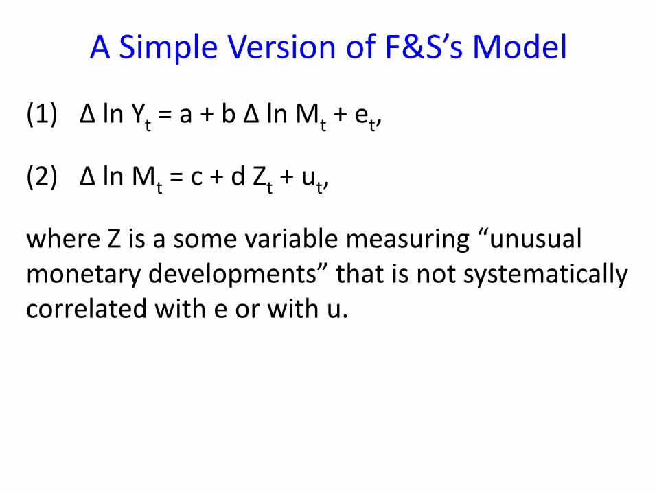
A Simple Version of F&S’s Model

(1) ∆ ln Yt = a + b ∆ ln Mt + et,

(2) ∆ ln Mt = c + d Zt + ut,

where Z is a some variable measuring “unusual monetary developments” that is not systematically correlated with e or with u.

A Simple Version of F&S’s Model (cont.) Substitute eq. (2) into eq. (1): ∆ ln Yt = a + b[c + dZt + ut] + et = (a + bc) + (bd)Zt + (but + et) = α + βZt + εt, where α ≡ a + bc, β ≡ bd, εt ≡ but + et.

Note that our assumptions about ε imply that it is not systematically correlated with Z.

A Simple Version of F&S’s Model (cont.) • We found ∆ ln Yt = α + βZt + εt, and that ε is not

systematically correlated with Z. • So we can estimate ∆ ln Yt = α + βZt + εt by an

OLS regression. • Note: This corresponds to the “direct” approach

to interpreting the results of experiments that we discussed last time.

• The alternative, IV, approach (which we won’t pursue) would be to estimate ∆ ln Yt = a + b ∆ ln Mt + et by IV, using Z as an instrument.

How Do Friedman and Schwartz Assess the Evidence from Their Four Crucial

Episodes?

What Do You Think?

III. ROMER AND ROMER

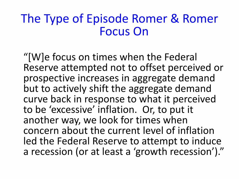
The Type of Episode Romer & Romer Focus On

“[W]e focus on times when the Federal Reserve attempted not to offset perceived or prospective increases in aggregate demand but to actively shift the aggregate demand curve back in response to what it perceived to be ‘excessive’ inflation. Or, to put it another way, we look for times when concern about the current level of inflation led the Federal Reserve to attempt to induce a recession (or at least a ‘growth recession’).”

• Less subjective

• Easier

Why Did Romer and Romer Focus on This Type of Episode, Rather than All

“Unusual” Monetary Developments?

Narrative Evidence of a Policy Shift in 1947 “It was [the] opinion [of the chief Federal Reserve economist present] that throughout the war and postwar period there had been too many fears of postwar deflation, … and that, although any downturn should be taken care of at the proper time, the important thing at the moment was to stop abnormal pressures on the inflationary side” (Minutes, 1947, p. 111)

The other Board economist at the meeting “thought there would and should be a mild recession” (Minutes, 1947, p. 112)

• October 1947

• September 1955

• December 1968

• April 1974

• August 1978

• October 1979

• (December 1988)

Dates of Shifts to Anti-Inflationary Monetary Policy

A Simple Version of R&R’s Implicit Model • Analogous to Friedman and Schwartz’s.

• Leads to ∆ ln Yt = α + βZt + εt, where Z is a measure of shifts to anti-inflationary monetary policy.

• Romer and Romer’s arguments about those shifts imply that we can estimate ∆ ln Yt = α + βZt + εt by an OLS regression.

The Unemployment Rate after “Romer & Romer Dates”

The Equation that Romer and Romer Estimate

• Uses industrial production as its measure of output.

• Allows monetary shocks to have delayed effects.

• Accounts for seasonal variation.

• Includes lagged values of output growth.

The Equation that Romer and Romer Estimate (cont.)

Estimated Impact of Shift to Anti-Inflationary Monetary Policy on Industrial Production

What Do You Think?

Estimated Impact of a Contractionary Monetary Shock in the Interwar Period on Industrial Production

(Shocks: 1/1920, 10/1930, 3/1931, 10/1931, 1/1937)

Estimated Impact of a Contractionary Monetary Shock in the Interwar Period on Industrial Production

(Shocks: 1/1920, 10/1931, 2/1933, 1/1937, 9/1941)