user location determination using delay and doppler
TRANSCRIPT
User Location Determination Using Delay andDoppler Measurements in LEO Satellite Systems
Y. Vasavada, D. Arur, C. Ravishankar, C. BarnettHughes Network Systems, Germantown, MD 20876
Abstract—Although an external Global Navigational SatelliteSystem (GNSS) solution is often relied upon for fixing the locationof user terminals (UTs), fixing the UT position autonomouslyin LEO satellite systems is a tractable problem which has asystem benefit. An autonomous solution comes to use if the GNSSsolution becomes unavailable either temporarily (e.g., due to adelay in initial GNSS position fix) or for prolonged periods (due tomajor outages or regulatory constraints), or if the system securitypolicies do not allow transmission of the user position over the air.In this paper, we describe two nonlinear root-finding algorithms(applicable either at the UT or at the satellite Gateway (GW))that take as the inputs the delay and Doppler offset measurementsfrom the physical layer receiver and generate an estimate of theuser location (and optionally velocity) as the output. Algorithmsimulation results suggest that a high accuracy estimate (in whichposition error exceeds 1 km in less than 10% cases) is possiblewhen UT has visibility to more than one satellite, while lessaccurate results (e.g., ∼ 20% chance of position errors exceeding2 km) are achievable in a single satellite scenario.
I. INTRODUCTION
In LEO satellite systems, the satellites and their beams movefast over the locations on the ground. Beams of the satellitepass over a location on the ground in the order of seconds andminutes, while the entire satellite coverage passes by a userlocation at the most in several tens of minutes [1]. Fast movingLEO constellation as viewed from the ground necessitatesaccurate and efficient inter-beam and inter-satellite handovermechanisms [2]. In addition, the high relative velocity betweenthe spacecraft and the UT on the ground results in largeDoppler and Doppler rates [3]. Knowledge of UT positionmitigates these system challanges by (i) reducing high Dopplerand Doppler rate uncertainties, thereby decreasing the re-ceiver implementation complexity, (ii) allowing a deterministicinter-beam and inter-satellite handoff, thereby simplifying themeasurement-driven real time handoff decision-making, (iii)increasing the efficiency of paging the user on the forwardlink control channel (this is because the Gateway, knowingthe position of the UT and those of the beams of the satellite,can limit sending the page message to only a few (one tothree) beams), and (iv) reducing the energy consumption atUT, translating to improved battery life.
While the position accuracy requirement for handover andpaging determination is on the order of kilometers, the re-quirement for the receiver timing/frequency search processis much tighter, i.e., on the order of hundreds of meters.Timing and Doppler uncertainties in LEO systems can be up
to ±0.33 µ-sec and ±2.5 ppb, respectively1, for 100 meterof position uncertainty. For large symbol rates and at highcarrier frequencies, uncertainties exceeding a few hundred ofmeters can translate to a significant computational load insignal acquisition.
A. Location Estimation in Satellite SystemsTheory and practice of position determination using navi-
gational satellites is well established, e.g., see [4], [5] for GPSand [6] for GLONASS and TRANSIT systems. Autonomousposition location in non-GNSS systems is feasible. Soleimaniand Liu describe position determination in a MEO satellite sys-tem in [7], and Kimura, et al., show a solution using two GEOsatellites in [8]. In [9], the authors describe the use of GPScombined with Time of Arrival (ToA) and Time Difference ofArrival (TDoA) of cellular signals. In [10], the authors com-bine the GPS measurements with the measurements over LEOsatellite links for position determination. In [11], the authorsdescribe a method for accurate determination of range andrange-rate to multiple satellites using ToA, TDoA and Dopplerfrequency shift measurements. A detailed treatment of positiondetermination using Globalstar LEO satellite constellation isprovided in [12], [13]. This paper follows an approach similarto that described in [12].
B. Contributions and OverviewThe main contribution of this paper is a detailed description
and performance evaluation of an iterative nonlinear algorithmthat can fix a total of six unknowns: coordinates of a terminal’sposition vector (longitude, latitude and height above Mean SeaLevel (MSL)), and coordinates of a terminal’s velocity vector(magnitude, longitude and latitude of the velocity vector interminal-specific East-North-Up (ENU) system).
The rest of the paper is organized as follows: Section IIprovides a detailed description of two different position de-termination algorithms. Section III presents simulation-basedperformance evaluation. A conclusion and a summary of thepaper are provided in Section IV.
II. ALGORITHMIC DESCRIPTION
Delay and Doppler offsets that the UT’s signal experienceson the LEO satellite link are nonlinear functions of the UTposition. Determination of UT position using these offsets isa nonlinear root finding problem. Two different methods forits solution are described next.
1This can be derived using the geometry of the path from the satellite tothe user position on the Earth. This derivation is not included here.
Milcom 2017 Track 4 - System Perspectives
978-1-5386-0595-0/17/$31.00 ©2017 IEEE 343
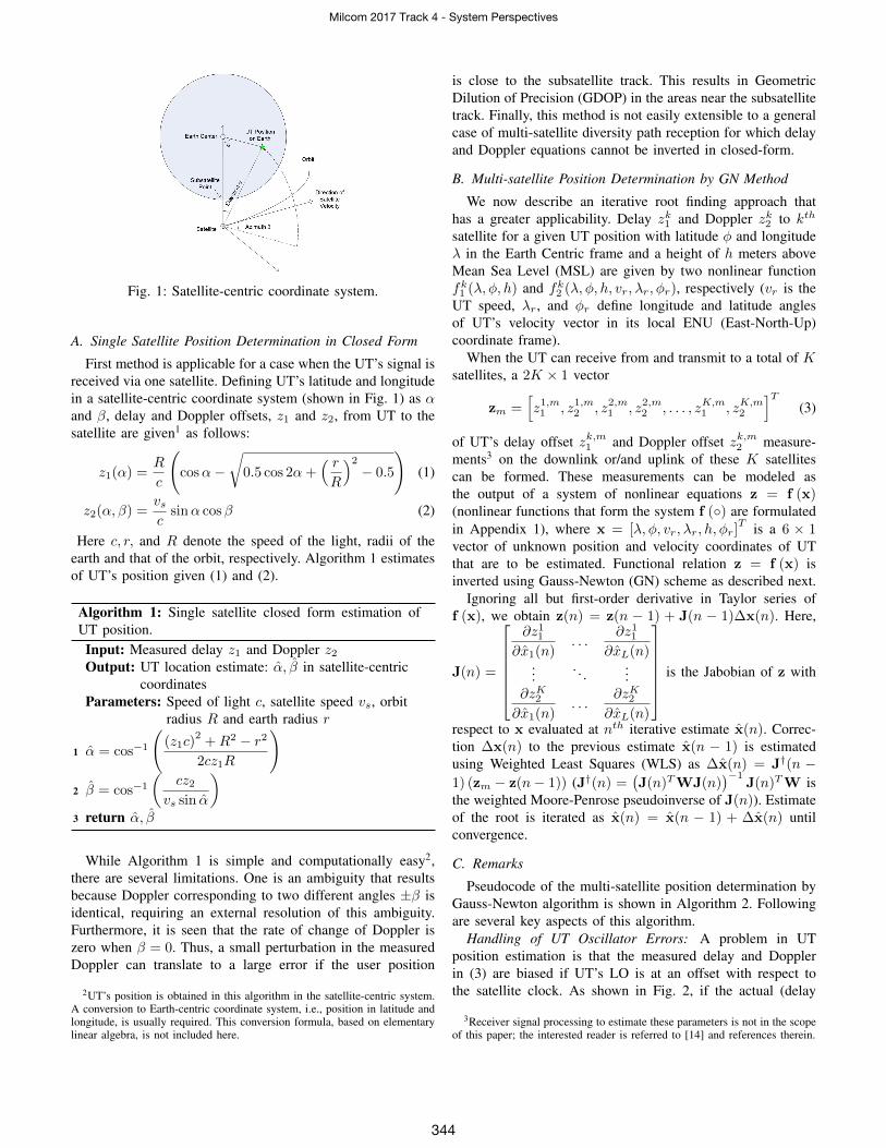
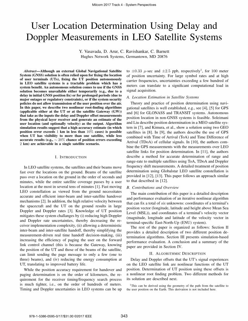
Fig. 1: Satellite-centric coordinate system.
A. Single Satellite Position Determination in Closed Form
First method is applicable for a case when the UT’s signal isreceived via one satellite. Defining UT’s latitude and longitudein a satellite-centric coordinate system (shown in Fig. 1) as αand β, delay and Doppler offsets, z1 and z2, from UT to thesatellite are given1 as follows:
z1(α) =R
c
(cosα−
√0.5 cos 2α+
( rR
)2− 0.5
)(1)
z2(α, β) =vsc
sinα cosβ (2)
Here c, r, and R denote the speed of the light, radii of theearth and that of the orbit, respectively. Algorithm 1 estimatesof UT’s position given (1) and (2).
Algorithm 1: Single satellite closed form estimation ofUT position.Input: Measured delay z1 and Doppler z2Output: UT location estimate: α, β in satellite-centric
coordinatesParameters: Speed of light c, satellite speed vs, orbit
radius R and earth radius r
1 α = cos−1
((z1c)
2+R2 − r2
2cz1R
)2 β = cos−1
(cz2
vs sin α
)3 return α, β
While Algorithm 1 is simple and computationally easy2,there are several limitations. One is an ambiguity that resultsbecause Doppler corresponding to two different angles ±β isidentical, requiring an external resolution of this ambiguity.Furthermore, it is seen that the rate of change of Doppler iszero when β = 0. Thus, a small perturbation in the measuredDoppler can translate to a large error if the user position
2UT’s position is obtained in this algorithm in the satellite-centric system.A conversion to Earth-centric coordinate system, i.e., position in latitude andlongitude, is usually required. This conversion formula, based on elementarylinear algebra, is not included here.
is close to the subsatellite track. This results in GeometricDilution of Precision (GDOP) in the areas near the subsatellitetrack. Finally, this method is not easily extensible to a generalcase of multi-satellite diversity path reception for which delayand Doppler equations cannot be inverted in closed-form.
B. Multi-satellite Position Determination by GN Method
We now describe an iterative root finding approach thathas a greater applicability. Delay zk1 and Doppler zk2 to kth
satellite for a given UT position with latitude φ and longitudeλ in the Earth Centric frame and a height of h meters aboveMean Sea Level (MSL) are given by two nonlinear functionfk1 (λ, φ, h) and fk2 (λ, φ, h, vr, λr, φr), respectively (vr is theUT speed, λr, and φr define longitude and latitude anglesof UT’s velocity vector in its local ENU (East-North-Up)coordinate frame).
When the UT can receive from and transmit to a total of Ksatellites, a 2K × 1 vector
zm =[z1,m1 , z1,m2 , z2,m1 , z2,m2 , . . . , zK,m
1 , zK,m2
]T(3)
of UT’s delay offset zk,m1 and Doppler offset zk,m2 measure-ments3 on the downlink or/and uplink of these K satellitescan be formed. These measurements can be modeled asthe output of a system of nonlinear equations z = f (x)(nonlinear functions that form the system f (◦) are formulatedin Appendix 1), where x = [λ, φ, vr, λr, h, φr]
T is a 6 × 1vector of unknown position and velocity coordinates of UTthat are to be estimated. Functional relation z = f (x) isinverted using Gauss-Newton (GN) scheme as described next.
Ignoring all but first-order derivative in Taylor series off (x), we obtain z(n) = z(n − 1) + J(n − 1)∆x(n). Here,
J(n) =
∂z11
∂x1(n). . .
∂z11∂xL(n)
.... . .
...∂zK2∂x1(n)
. . .∂zK2∂xL(n)
is the Jabobian of z with
respect to x evaluated at nth iterative estimate x(n). Correc-tion ∆x(n) to the previous estimate x(n − 1) is estimatedusing Weighted Least Squares (WLS) as ∆x(n) = J†(n −1) (zm − z(n− 1)) (J†(n) =
(J(n)TWJ(n)
)−1J(n)TW is
the weighted Moore-Penrose pseudoinverse of J(n)). Estimateof the root is iterated as x(n) = x(n − 1) + ∆x(n) untilconvergence.
C. Remarks
Pseudocode of the multi-satellite position determination byGauss-Newton algorithm is shown in Algorithm 2. Followingare several key aspects of this algorithm.
Handling of UT Oscillator Errors: A problem in UTposition estimation is that the measured delay and Dopplerin (3) are biased if UT’s LO is at an offset with respect tothe satellite clock. As shown in Fig. 2, if the actual (delay
3Receiver signal processing to estimate these parameters is not in the scopeof this paper; the interested reader is referred to [14] and references therein.
Milcom 2017 Track 4 - System Perspectives
344
Algorithm 2: Gauss-Newton (GN) Algorithm for single ormultiple satellite estimation of UT position and velocity.Input: Measured delay and Doppler vector in Eq.(3);
number L of unknown parameters to be estimatedOutput: UT location and velocity estimates:
x =[λ, φ, vr, λr, h, φr
]TParameters: satellite (ephemeris) position and velocity
vectors, algorithm convergence thresholdparameters εA and εB , and maximumnumber of algorithm iterations nmax
1 n← 0, en ← εA + 1, condNumber ← 1
2 x(n) =[λ(n), φ(n), vr(n), λr(n), h, φr(n)
]T← initial
seed3 while en > εA and condNumber > εB and n < nmax
do4 z(n) = f(x(n))5 e(n) = zm − z(n); en = eT (n)e(n)
6 J(n)← ∂z(n)
∂x(n)7 condNumber ← RCOND(J(n)TWJ(n))8 x(n+ 1) = x(n) +
(J(n)TWJ(n)
)−1J(n)TWe(n)
9 n← n+ 1
10 return x(n)
or Doppler) offset on the satellite link is a, the UT, withan oscillator that has synchronization error of b relative tothe satellite, measures an offset of a − b instead of a. Thereare several alternatives to resolve this oscillator error. Firstscheme relies on either a separate synchronization scheme thataligns the clocks at the satellite and the UT, or a high-fidelityoscillator at the UT for which the error b is negligible. Secondoption is to modify (3) so that the vector zm represents thedifferential delays and Doppler values instead of absolute. Byusing TDoA and Doppler DoA for kth satellite relative toa reference satellite, the UT clock error b can be canceled.Finally, the third option is to measure the timing and frequencyoffsets on the return link at the satellite, which equals a + bas illustrated in Fig. 2. UT can report its measurement a− b,and the GW can separate a and b using its measurement ofa+ b and value a− b that UT reports [12].
Number L of Estimated Variables: In Algorithm 2, thenumber L of unknowns to be estimated is a variable. To avoidan underdetermined set of nonlinear equations, L is requiredto be less than or equal to the cardinality of zm, which is 2Kwith K visible satellites. If only UT’s position coordinatesare to be estimated, L is set to two and the first two variablesof x, i.e., UT’s position φ and λ, are estimated by the GNAlgorithm. If UT’s velocity coordinates are also required tobe estimated, K is required to be at least 2, L is set to 4,and first four variables of x are estimated by the algorithm.Finally, if K ≥ 3, all six components of UT’s position andvelocity vectors can be estimated.
Fig. 2: Proportionality of the offsets measured on the downlinkand uplink to a − b, and a + b, respectively, where a is thelink Doppler (or delay) and b is the UT oscillator offset.
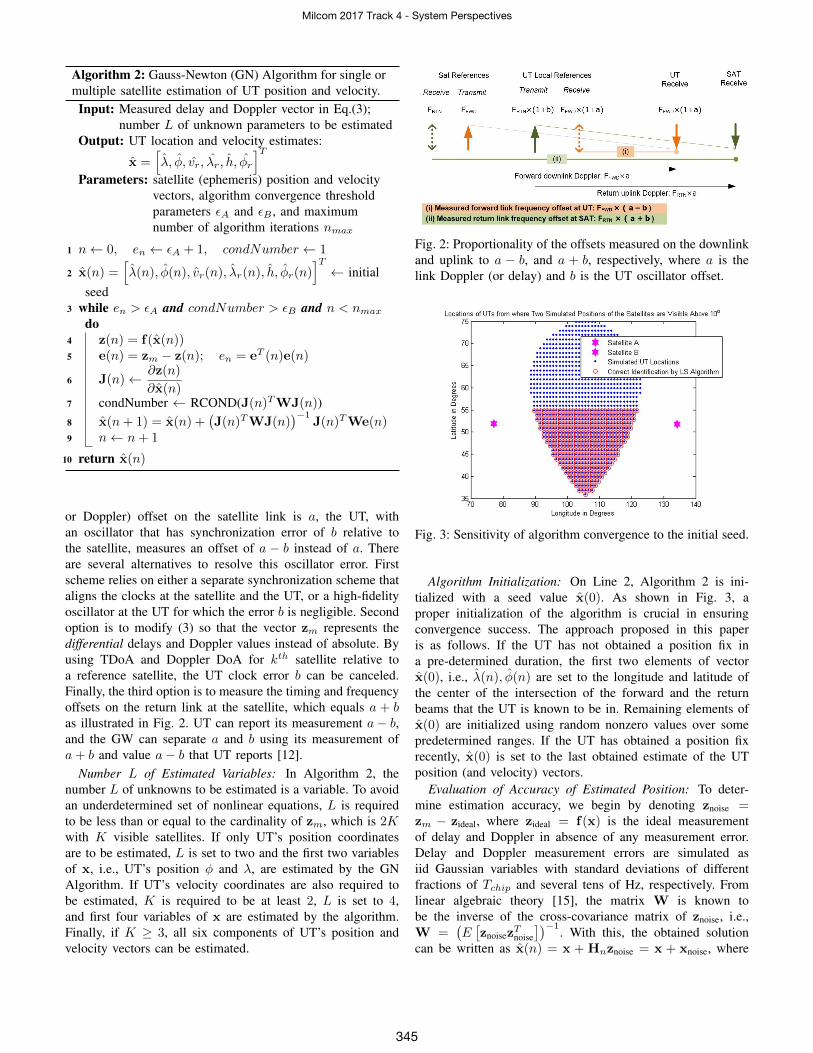
Fig. 3: Sensitivity of algorithm convergence to the initial seed.
Algorithm Initialization: On Line 2, Algorithm 2 is ini-tialized with a seed value x(0). As shown in Fig. 3, aproper initialization of the algorithm is crucial in ensuringconvergence success. The approach proposed in this paperis as follows. If the UT has not obtained a position fix ina pre-determined duration, the first two elements of vectorx(0), i.e., λ(n), φ(n) are set to the longitude and latitude ofthe center of the intersection of the forward and the returnbeams that the UT is known to be in. Remaining elements ofx(0) are initialized using random nonzero values over somepredetermined ranges. If the UT has obtained a position fixrecently, x(0) is set to the last obtained estimate of the UTposition (and velocity) vectors.
Evaluation of Accuracy of Estimated Position: To deter-mine estimation accuracy, we begin by denoting znoise =zm − zideal, where zideal = f(x) is the ideal measurementof delay and Doppler in absence of any measurement error.Delay and Doppler measurement errors are simulated asiid Gaussian variables with standard deviations of differentfractions of Tchip and several tens of Hz, respectively. Fromlinear algebraic theory [15], the matrix W is known tobe the inverse of the cross-covariance matrix of znoise, i.e.,W =
(E[znoisez
Tnoise
])−1. With this, the obtained solution
can be written as x(n) = x + Hnznoise = x + xnoise, where
Milcom 2017 Track 4 - System Perspectives
345
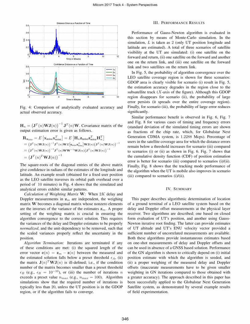
Fig. 4: Comparison of analytically evaluated accuracy andactual observed accuracy.
Hn =(JT (n)WJ(n)
)−1JT (n)W. Covariance matrix of the
output estimation error is given as follows.
Rxnoise = E[xnoisex
Tnoise
]= E
[Hnznoisez
TnoiseH
Tn
]= (JT (n)WJ(n))
−1JT (n)WE[znoisez
Tnoise]WJ(n)(JT (n)WJ(n))
−1
= (JT (n)WJ(n))−1
JT (n)WW−1WJ(n)(JT (n)WJ(n))−1
=(JT (n)TWJ(n)
)−1The square-roots of the diagonal entries of the above matrixgive confidence in radians of the estimates of the longitude andlatitude. An example result (obtained for a fixed user positionas the LEO satellite traverses its orbital path overhead over aperiod of 10 minutes) in Fig. 4 shows that the simulated andanalytical errors exhibit similar patterns.
Calculation of Weighting Matrix W: When 2K delay andDoppler measurements in zm are independent, the weighingmatrix W becomes a diagonal matrix whose nonzero elementsare the inverses of the variance of the estimates zm. A propersetting of the weighing matrix is crucial in ensuring thealgorithm convergence to the correct solution. This requiresthe variances of the delay and Doppler estimates to be properlynormalized, and the unit-dependency to be removed, such thatthe scaled variances properly reflect the uncertainty in theposition.
Algorithm Termination: Iterations are terminated if anyof these conditions are met: (i) the squared length of theerror vector e(n) = zm − z(n) between the measured andthe estimated solution falls below a preset threshold εA, (ii)the matrix J(n)TWJ(n) is ill-defined; i.e., if the conditionnumber of the matrix becomes smaller than a preset thresholdεB (e.g., εB = 10−10), or (iii) the number of iterations nexceeds a preset value nmax (e.g., nmax = 100). Algorithmsimulations show that the required number of iterations istypically less than 20, unless the UT position is in the GDOPregion, or if the algorithm fails to converge.
III. PERFORMANCE RESULTS
Performance of Gauss-Newton algorithm is evaluated inthis section by means of Monte-Carlo simulation. In thesimulation, L is taken as 2 (only UT position longitude andlatitude are estimated). A total of three scenarios of satellitevisibility at the UT are simulated: (i) one satellite on theforward and return, (ii) one satellite on the forward and anotherone on the return link, and (iii) one satellite on the forwardlink and two satellites on the return link.
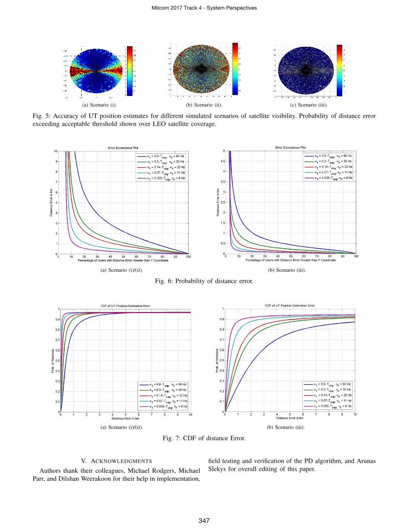
In Fig. 5, the probability of algorithm convergence over theLEO satellite coverage region is shown for three scenarios:GDOP area is clearly visible for scenario (i) result in Fig. 5,the estimation accuracy degrades in the region close to thesubsatellite track (X-axis of the figure). Although this GDOPregion disappears for scenario (ii), the probability of largeerror persists (it spreads over the entire coverage region).Finally, for scenario (iii), the probability of large error reducessignificantly.
Similar performance benefit is observed in Fig. 6, Fig. 7and Fig. 8 for various cases of timing and frequency errors(standard deviation of the simulated timing errors are shownas fractions of the chip rate, which, for Globalstar NextGeneration CDMA system, is 1.2288 Mcps). Percentage ofusers in the satellite coverage area for which the distance errorsremain below a threshold increases for scenario (iii) comparedto scenarios (i) or (ii) as shown in Fig. 6. Fig. 7 shows thatthe cumulative density function (CDF) of position estimationerror is better for scenario (iii) compared to scenarios (i)/(ii).Finally, Fig. 8 shows that the tracking mode performance ofthe algorithm when the UT is mobile also improves in scenario(iii) compared to scenarios (i)/(ii).
IV. SUMMARY
This paper describes algorithmic determination of locationof a ground terminal of a LEO satellite system based on thedelay and Doppler offset measurements at the physical layerreceiver. Two algorithms are described; one based on closedform evaluation of UT’s position, and another using Gauss-Newton iterative root finding. The latter can provide estimatesof UT altitude and UT’s ENU velocity vector provided asufficient number of uncorrelated measurements are available.Both these algorithms provide instantaneous estimates basedon one-shot measurements of delay and Doppler offsets andcan be used in absence of a GNSS based solution. Performanceof the GN algorithm is shown to critically depend on (i) initialposition estimate with which the algorithm is seeded, and(ii) a proper weighing of the measured delay and Doppleroffsets (inaccurate measurements have to be given smallerweighting in GN iterations compared to those obtained witha greater accuracy). The approach described in this paper hasbeen successfully applied to the Globalstar Next GenerationSatellite system, as demonstrated by several example resultsof field experimentation.
Milcom 2017 Track 4 - System Perspectives
346
(a) Scenario (i). (b) Scenario (ii). (c) Scenario (iii).
Fig. 5: Accuracy of UT position estimates for different simulated scenarios of satellite visibility. Probability of distance errorexceeding acceptable threshold shown over LEO satellite coverage.
(a) Scenario (i)/(ii). (b) Scenario (iii).
Fig. 6: Probability of distance error.
(a) Scenario (i)/(ii). (b) Scenario (iii).
Fig. 7: CDF of distance Error.
V. ACKNOWLEDGMENTS
Authors thank their colleagues, Michael Rodgers, MichaelParr, and Dilshan Weerakoon for their help in implementation,
field testing and verification of the PD algorithm, and ArunasSlekys for overall editing of this paper.
Milcom 2017 Track 4 - System Perspectives
347
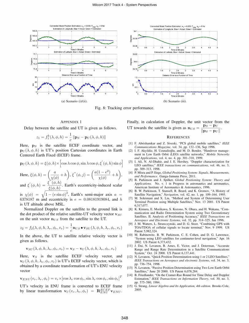
(a) Scenario (i)/(ii). (b) Scenario (iii).
Fig. 8: Tracking error performance.
APPENDIX 1
Delay between the satellite and UT is given as follows.
z1 = fk1 (λ, φ, h) =1
c‖pS − pU (λ, φ, h)‖
Here, pS is the satellite ECEF coordinate vector, andpU (λ, φ, h) is UT’s position Cartesian coordinates in EarthCentered Earth Fixed (ECEF) frame.
pU (λ, φ, h) = ξ(φ, h)×[cosλ cosφ, sinλ cosφ, ξ
′(φ, h) sinφ
]Here, ξ(φ, h) =
(a
χ(φ)+ h
), ξ′′(φ, j) =
(a(1− e2)
χ(φ)+ h
),
and ξ′(φ, h) =
ξ′′(φ, h)
ξ(φ, h). Earth’s eccentricity-induced scalar
is χ(φ) =
√1− (e sinφ)
2, Earth’s semi-major axis a =6378187 m and eccentricity is e = 0.08181919084, and his UT altitude above MSL.
Normalized Doppler on the satellite to the ground link isthe dot product of the relative satellite-UT velocity vector vSU
on the unit vector nUS from the satellite to the UT.
z2 = f2(λ, φ, h, λr, φr, vr) =1
cnUS •vSU (λ, φ, h, λr, φr, vr)
In the above, the UT to satellite relative velocity vector isgiven as follows.
vSU (λ, φ, h, λr, φr, vr) = vS − vU (λ, φ, h, λr, φr, vr)
Here, vS is the satellite ECEF velocity vector, andvU (λ, φ, h, λr, φr, vr) is UT’s ECEF velocity vector, which isobtained by a coordinate transformation of UT’s ENU velocityvector
vENU (vr, λr, φr) = vr×[cosλr cosφr, sinλr cosφr, sinφr]T
UT’s velocity in ENU frame is converted to ECEF frameby linear transformation vU (vr, λr, φr) = RECEF
ENU vENU .
Finally, in calculation of Doppler, the unit vector from theUT towards the satellite is given as nUS =
pS − pU
‖pS − pU‖.
REFERENCES
[1] F. Abrishamkar and Z. Siveski, “PCS global mobile satellites,” IEEECommunications Magazine, vol. 34, pp. 132–136, Sep 1996.
[2] I. F. Akyildiz, H. Uzunalioglu, and M. D. Bender, “Handover manage-ment in Low Earth Orbit (LEO) satellite networks,” Mobile Networksand Applications, vol. 4, no. 4, pp. 301–310, 1999.
[3] I. Ali, N. Al-Dhahir, and J. E. Hershey, “Doppler characterization forLEO satellites,” IEEE transactions on communications, vol. 46, no. 3,pp. 309–313, 1998.
[4] P. Misra and P. Enge, Global Positioning System: Signals, Measurements,and Performance. Ganga-Jamuna Press, 2011.
[5] B. Parkinson and J. Spilker, Global Positioning System: Theory andApplications. No. v. 1 in Progress in astronautics and aeronautics,American Institute of Aeronautics & Astronautics, 1996.
[6] B. W. Parkinson, T. Stansell, R. Beard, and K. Gromov, “A History ofSatellite Navigation,” Navigation, vol. 42, no. 1, pp. 109–164, 1995.
[7] M. Soleimani and X. Liu, “Method and System of Determining UserTerminal Position using Multiple Satellites,” Nov. 13 2001. US Patent6,317,077.
[8] K. Kimura, E. Morikawa, S. Kozono, N. Obara, and H. Wakana, “Com-munication and Radio Determination System using Two GeostationarySatellites. II. Analysis of Positioning Accuracy,” IEEE Transactions onAerospace and Electronic Systems, vol. 32, pp. 314–325, Jan 1996.
[9] J. M. Watters, L. Strawczynski, and D. G. Steer, “Combining GPS withTOA/TDOA of cellular signals to locate terminal,” Nov. 9 1999. USPatent 5,982,324.
[10] M. Rabinowitz, B. W. Parkinson, C. E. Cohen, and D. G. Lawrence,“System using LEO satellites for centimeter-level navigation,” Apr. 162002. US Patent 6,373,432.
[11] J. Dai, N. Levanon, B. Ames, E. Victor, and J. Determan, “AccurateRange and Range Rate Determination in a Satellite CommunicationsSystem,” Oct. 24 2000. US Patent 6,137,441.
[12] N. Levanon, “Quick Position Determination using 1 or 2 LEO Satellites,”IEEE Transactions on Aerospace and electronic Systems, vol. 34, no. 3,pp. 736–754, 1998.
[13] N. Levanon, “Passive Position Determination using Two Low Earth OrbitSatellites,” June 20 2000. US Patent 6,078,284.
[14] B. Friedlander, “On the Cramer-Rao Bound for Time Delay and DopplerEstimation,” IEEE Transactions on Information Theory, vol. 30, no. 3,pp. 575–580, 1984.
[15] G. Strang, Linear Algebra and Its Application, 4th edition. Brooks Cole,2005.
Milcom 2017 Track 4 - System Perspectives
348