using disaggregate demand models in operations … disaggregate demand models in operations ......
TRANSCRIPT

Using disaggregate demand models in operationsresearch
Michel Bierlaire Meritxell Pacheco
Transport and Mobility LaboratorySchool of Architecture, Civil and Environmental Engineering
Ecole Polytechnique Federale de Lausanne
January 5, 2017
Michel Bierlaire, Meritxell Pacheco (EPFL) Choice models and MILP January 5, 2017 1 / 65

Demand and supply
Outline
1 Demand and supply
2 Disaggregate demand models
3 Choice-based optimizationApplications
4 A generic framework
5 A simple exampleExample: one theaterExample: two theatersExample: two theaters with capacities
6 Parking management7 Conclusion
Michel Bierlaire, Meritxell Pacheco (EPFL) Choice models and MILP January 5, 2017 2 / 65

Demand and supply
Demand models
Supply = infrastructure
Demand = behavior, choices
Congestion = mismatch
Michel Bierlaire, Meritxell Pacheco (EPFL) Choice models and MILP January 5, 2017 3 / 65

Demand and supply
Demand models
Usually in OR:
optimization of the supply
for a given (fixed) demand
Michel Bierlaire, Meritxell Pacheco (EPFL) Choice models and MILP January 5, 2017 4 / 65

Demand and supply
Aggregate demand
Homogeneous population
Identical behavior
Price (P) and quantity (Q)
Demand functions: P = f (Q)
Inverse demand: Q = f −1(P)
Michel Bierlaire, Meritxell Pacheco (EPFL) Choice models and MILP January 5, 2017 5 / 65

Demand and supply
Disaggregate demand
Heterogeneous population
Different behaviors
Many variables:
Attributes: price, travel time,reliability, frequency, etc.Characteristics: age, income,education, etc.
Complex demand/inversedemand functions.
Michel Bierlaire, Meritxell Pacheco (EPFL) Choice models and MILP January 5, 2017 6 / 65
Demand and supply
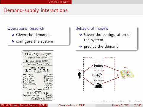
Demand-supply interactions
Operations Research
Given the demand...
configure the system
Behavioral models
Given the configuration ofthe system...
predict the demand
Michel Bierlaire, Meritxell Pacheco (EPFL) Choice models and MILP January 5, 2017 7 / 65

Demand and supply
Demand-supply interactions
Multi-objective optimization
Minimize costs Maximize satisfaction
Michel Bierlaire, Meritxell Pacheco (EPFL) Choice models and MILP January 5, 2017 8 / 65

Disaggregate demand models
Outline
1 Demand and supply
2 Disaggregate demand models
3 Choice-based optimizationApplications
4 A generic framework
5 A simple exampleExample: one theaterExample: two theatersExample: two theaters with capacities
6 Parking management7 Conclusion
Michel Bierlaire, Meritxell Pacheco (EPFL) Choice models and MILP January 5, 2017 9 / 65
Disaggregate demand models
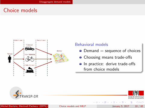
Choice models
Behavioral models
Demand = sequence of choices
Choosing means trade-offs
In practice: derive trade-offsfrom choice models
Michel Bierlaire, Meritxell Pacheco (EPFL) Choice models and MILP January 5, 2017 10 / 65

Disaggregate demand models
Choice models
Theoretical foundations
Random utility theory
Choice set: Cn
yin = 1 if i ∈ Cn, 0 if not
Logit model:
P(i |Cn) =yine
Vin
∑
j∈C yjneVjn
2000
Michel Bierlaire, Meritxell Pacheco (EPFL) Choice models and MILP January 5, 2017 11 / 65
Disaggregate demand models
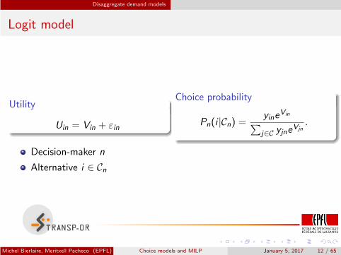
Logit model
Utility
Uin = Vin + εin
Choice probability
Pn(i |Cn) =yine
Vin
∑
j∈C yjneVjn
.
Decision-maker n
Alternative i ∈ Cn
Michel Bierlaire, Meritxell Pacheco (EPFL) Choice models and MILP January 5, 2017 12 / 65

Disaggregate demand models
Variables: xin = (zin, sn)
Attributes of alternative i : zin
Cost / price
Travel time
Waiting time
Level of comfort
Number of transfers
Late/early arrival
etc.
Characteristics of decision-maker n:sn
Income
Age
Sex
Trip purpose
Car ownership
Education
Profession
etc.
Michel Bierlaire, Meritxell Pacheco (EPFL) Choice models and MILP January 5, 2017 13 / 65
Disaggregate demand models
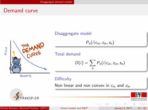
Demand curve
Disaggregate model
Pn(i |cin, zin, sn)
Total demand
D(i) =∑
n
Pn(i |cin, zin, sn)
Difficulty
Non linear and non convex in cin and zin
Michel Bierlaire, Meritxell Pacheco (EPFL) Choice models and MILP January 5, 2017 14 / 65
Choice-based optimization
Outline
1 Demand and supply
2 Disaggregate demand models
3 Choice-based optimizationApplications
4 A generic framework
5 A simple exampleExample: one theaterExample: two theatersExample: two theaters with capacities
6 Parking management7 Conclusion
Michel Bierlaire, Meritxell Pacheco (EPFL) Choice models and MILP January 5, 2017 15 / 65

Choice-based optimization
Choice-Based Optimization Models
Benefits
Merging supply and demand aspect of planning
Accounting for the heterogeneity of demand
Dealing with complex substitution patterns
Investigation of demand elasticity against its main driver (e.g. price)
Challenges
Nonlinearity and nonconvexity
Assumptions for simple models (logit) may be inappropriate
Advanced demand models have no closed-form
Endogeneity: same variable(s) both in the demand function and thecost function
Michel Bierlaire, Meritxell Pacheco (EPFL) Choice models and MILP January 5, 2017 16 / 65

Choice-based optimization Applications
Stochastic traffic assignment
Features
Nash equilibrium
Flow problem
Demand: path choice
Supply: capacity
Michel Bierlaire, Meritxell Pacheco (EPFL) Choice models and MILP January 5, 2017 17 / 65

Choice-based optimization Applications
Selected literature
[Dial, 1971]: logit
[Daganzo and Sheffi, 1977]: probit
[Fisk, 1980]: logit
[Bekhor and Prashker, 2001]: cross-nested logit
and many others...
Michel Bierlaire, Meritxell Pacheco (EPFL) Choice models and MILP January 5, 2017 18 / 65

Choice-based optimization Applications
Revenue management
Features
Stackelberg game
Bi-level optimization
Demand: purchase
Supply: price and capacity
Michel Bierlaire, Meritxell Pacheco (EPFL) Choice models and MILP January 5, 2017 19 / 65
Choice-based optimization Applications
Selected literature
[Labbe et al., 1998]: bi-level programming
[Andersson, 1998]: choice-based RM
[Talluri and Van Ryzin, 2004]: choice-based RM
[Gilbert et al., 2014a]: logit
[Gilbert et al., 2014b]: mixed logit
[Azadeh et al., 2015]: global optimization
and many others...
Michel Bierlaire, Meritxell Pacheco (EPFL) Choice models and MILP January 5, 2017 20 / 65

Choice-based optimization Applications
Facility location problem
Features
Competitive market
Opening a facility impact the costs
Opening a facility impact the demand
Decision variables: availability of thealternatives
Pn(i |Cn) =yine
Vin
∑
j∈C yjneVjn
.
Michel Bierlaire, Meritxell Pacheco (EPFL) Choice models and MILP January 5, 2017 21 / 65

Choice-based optimization Applications
Selected literature
[Hakimi, 1990]: competitive location (heuristics)
[Benati, 1999]: competitive location (B & B, Lagrangian relaxation,submodularity)
[Serra and Colome, 2001]: competitive location (heuristics)
[Marianov et al., 2008]: competitive location (heuristic)
[Haase and Muller, 2013]: school location (simulation-based)
Michel Bierlaire, Meritxell Pacheco (EPFL) Choice models and MILP January 5, 2017 22 / 65

A generic framework
Outline
1 Demand and supply
2 Disaggregate demand models
3 Choice-based optimizationApplications
4 A generic framework
5 A simple exampleExample: one theaterExample: two theatersExample: two theaters with capacities
6 Parking management7 Conclusion
Michel Bierlaire, Meritxell Pacheco (EPFL) Choice models and MILP January 5, 2017 23 / 65
A generic framework
The main idea
Linearization
Hopeless to linearize the logit formula (we tried...)
First principles
Each customer solves an optimization problem
Solution
Use the utility and not the probability
Michel Bierlaire, Meritxell Pacheco (EPFL) Choice models and MILP January 5, 2017 24 / 65

A generic framework
A linear formulation
Utility function
Uin = Vin + εin =∑
k
βkxink + f (zin) + εin.
Simulation
Assume a distribution for εin
E.g. logit: i.i.d. extreme value
Draw R realizations ξinr ,r = 1, . . . ,R
The choice problem becomesdeterministic
Michel Bierlaire, Meritxell Pacheco (EPFL) Choice models and MILP January 5, 2017 25 / 65
A generic framework
Scenarios
Draws
Draw R realizations ξinr , r = 1, . . . ,R
We obtain R scenarios
Uinr =∑
k
βkxink + f (zin) + ξinr .
For each scenario r , we can identify the largest utility.
It corresponds to the chosen alternative.
Michel Bierlaire, Meritxell Pacheco (EPFL) Choice models and MILP January 5, 2017 26 / 65
A generic framework
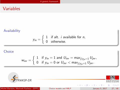
Variables
Availability
yin =
{
1 if alt. i available for n,0 otherwise.
Choice
winr =
{
1 if yin = 1 and Uinr = maxj |yjn=1 Ujnr ,
0 if yin = 0 or Uinr < maxj |yjn=1 Ujnr .
Michel Bierlaire, Meritxell Pacheco (EPFL) Choice models and MILP January 5, 2017 27 / 65

A generic framework
Capacities
Demand may exceed supply
Each alternative i can bechosen by maximum ciindividuals.
An exogenous priority list isavailable.
The numbering of individuals isconsistent with their priority.
Michel Bierlaire, Meritxell Pacheco (EPFL) Choice models and MILP January 5, 2017 28 / 65
A generic framework
Priority list
Application dependent
First in, first out
Frequent travelers
Subscribers
...
In this framework
The list of customers must be sorted
Michel Bierlaire, Meritxell Pacheco (EPFL) Choice models and MILP January 5, 2017 29 / 65

A generic framework
Capacities
Variables
yin: decision of the operator
yinr : availability
Constraints
∑
i∈C
winr = 1 ∀n, r .
N∑
n=1
winr ≤ ci ∀i , n, r .
winr ≤ yinr ∀i , n, r .
yinr ≤ yin ∀i , n, r .
yi(n+1)r ≤ yinr ∀i , n, r .
Michel Bierlaire, Meritxell Pacheco (EPFL) Choice models and MILP January 5, 2017 30 / 65
A generic framework
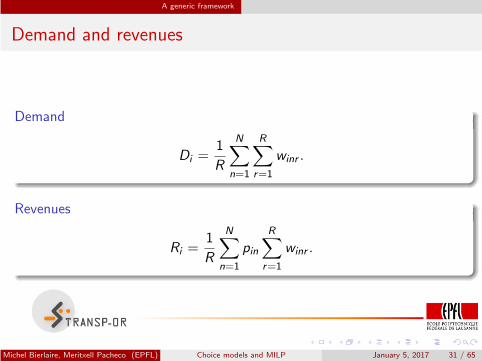
Demand and revenues
Demand
Di =1
R
N∑
n=1
R∑
r=1
winr .
Revenues
Ri =1
R
N∑
n=1
pin
R∑
r=1
winr .
Michel Bierlaire, Meritxell Pacheco (EPFL) Choice models and MILP January 5, 2017 31 / 65
A generic framework
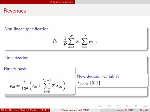
Revenues
Non linear specification
Ri =1
R
N∑
n=1
pin
R∑
r=1
winr .
Linearization
Binary basis
pin =1
10d
(
ℓin +
Lin−1∑
ℓ=0
2ℓλinℓ
)
.
New decision variables
λinℓ ∈ {0, 1}
Michel Bierlaire, Meritxell Pacheco (EPFL) Choice models and MILP January 5, 2017 32 / 65
A generic framework
References
Technical report: [Bierlaire and Azadeh, 2016]
Conference proceeding: [Pacheco et al., 2016]
Michel Bierlaire, Meritxell Pacheco (EPFL) Choice models and MILP January 5, 2017 33 / 65

A simple example
Outline
1 Demand and supply
2 Disaggregate demand models
3 Choice-based optimizationApplications
4 A generic framework
5 A simple exampleExample: one theaterExample: two theatersExample: two theaters with capacities
6 Parking management7 Conclusion
Michel Bierlaire, Meritxell Pacheco (EPFL) Choice models and MILP January 5, 2017 34 / 65

A simple example
A simple example
Data
C: set of movies
Population of N individuals
Utility function:Uin = βinpin + f (zin) + εin
Decision variables
What movies to propose? yi
What price? pin
Michel Bierlaire, Meritxell Pacheco (EPFL) Choice models and MILP January 5, 2017 35 / 65

A simple example Example: one theater
Back to the example: pricing
Data
Two alternatives: my theater (m) andthe competition (c)
We assume an homogeneouspopulation of N individuals
Uc = 0 + εc
Um = βcpm + εm
βc < 0
Logit model: εm i.i.d. EV
Michel Bierlaire, Meritxell Pacheco (EPFL) Choice models and MILP January 5, 2017 36 / 65

A simple example Example: one theater
Demand and revenues
0
0.1
0.2
0.3
0.4
0.5
0.6
0.7
0.8
0.9
1
0 0.2 0.4 0.6 0.8 10
0.02
0.04
0.06
0.08
0.1
0.12
0.14
0.16
Dem
and
Revenues
Price
RevenuesDemand
Michel Bierlaire, Meritxell Pacheco (EPFL) Choice models and MILP January 5, 2017 37 / 65

A simple example Example: one theater
Optimization (with GLPK)
Data
N = 1
R = 100
Um = −10pm + 3
Prices: 0.10, 0.20, 0.30, 0.40,0.50
Results
Optimum price: 0.3
Demand: 56%
Revenues: 0.168
Michel Bierlaire, Meritxell Pacheco (EPFL) Choice models and MILP January 5, 2017 38 / 65

A simple example Example: one theater
Heterogeneous population
Two groups in the population
Uin = −βnpi + cn
Young fans: 2/3
β1 = −10, c1 = 3
Others: 1/3
β1 = −0.9, c1 = 0
Michel Bierlaire, Meritxell Pacheco (EPFL) Choice models and MILP January 5, 2017 39 / 65

A simple example Example: one theater
Demand and revenues
0
0.2
0.4
0.6
0.8
1
0 0.5 1 1.5 20
0.05
0.1
0.15
0.2
0.25
0.3
0.35
0.4
0.45
Dem
and
Revenues
Price
RevenuesDemand
Young fansOthers
Michel Bierlaire, Meritxell Pacheco (EPFL) Choice models and MILP January 5, 2017 40 / 65
A simple example Example: one theater
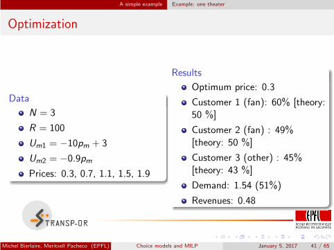
Optimization
Data
N = 3
R = 100
Um1 = −10pm + 3
Um2 = −0.9pm
Prices: 0.3, 0.7, 1.1, 1.5, 1.9
Results
Optimum price: 0.3
Customer 1 (fan): 60% [theory:50 %]
Customer 2 (fan) : 49%[theory: 50 %]
Customer 3 (other) : 45%[theory: 43 %]
Demand: 1.54 (51%)
Revenues: 0.48
Michel Bierlaire, Meritxell Pacheco (EPFL) Choice models and MILP January 5, 2017 41 / 65

A simple example Example: two theaters
Two theaters, different types of films
Michel Bierlaire, Meritxell Pacheco (EPFL) Choice models and MILP January 5, 2017 42 / 65

A simple example Example: two theaters
Two theaters, different types of films
Theater m
Expensive
Star Wars Episode VII
Theater k
Cheap
Tinker Tailor Soldier Spy
Heterogeneous demand
Two third of the population is young (price sensitive)
One third of the population is old (less price sensitive)
Michel Bierlaire, Meritxell Pacheco (EPFL) Choice models and MILP January 5, 2017 43 / 65
A simple example Example: two theaters
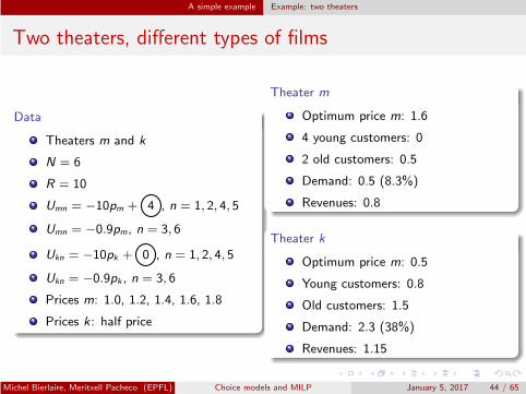
Two theaters, different types of films
Data
Theaters m and k
N = 6
R = 10
Umn = −10pm + 4 , n = 1, 2, 4, 5
Umn = −0.9pm, n = 3, 6
Ukn = −10pk + 0 , n = 1, 2, 4, 5
Ukn = −0.9pk , n = 3, 6
Prices m: 1.0, 1.2, 1.4, 1.6, 1.8
Prices k: half price
Theater m
Optimum price m: 1.6
4 young customers: 0
2 old customers: 0.5
Demand: 0.5 (8.3%)
Revenues: 0.8
Theater k
Optimum price m: 0.5
Young customers: 0.8
Old customers: 1.5
Demand: 2.3 (38%)
Revenues: 1.15
Michel Bierlaire, Meritxell Pacheco (EPFL) Choice models and MILP January 5, 2017 44 / 65

A simple example Example: two theaters
Two theaters, same type of films
Theater m
Expensive
Star Wars Episode VII
Theater k
Cheap
Star Wars Episode VIII
Heterogeneous demand
Two third of the population is young (price sensitive)
One third of the population is old (less price sensitive)
Michel Bierlaire, Meritxell Pacheco (EPFL) Choice models and MILP January 5, 2017 45 / 65
A simple example Example: two theaters
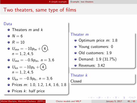
Two theaters, same type of films
Data
Theaters m and k
N = 6
R = 10
Umn = −10pm + 4 ,n = 1, 2, 4, 5
Umn = −0.9pm, n = 3, 6
Ukn = −10pk + 4 ,n = 1, 2, 4, 5
Ukn = −0.9pk , n = 3, 6
Prices m: 1.0, 1.2, 1.4, 1.6, 1.8
Prices k : half price
Theater m
Optimum price m: 1.8
Young customers: 0
Old customers: 1.9
Demand: 1.9 (31.7%)
Revenues: 3.42
Theater k
Closed
Michel Bierlaire, Meritxell Pacheco (EPFL) Choice models and MILP January 5, 2017 46 / 65

A simple example Example: two theaters with capacities
Two theaters with capacity, different types of films
Data
Theaters m and k
Capacity: 2
N = 6
R = 5
Umn = −10pm + 4, n = 1, 2, 4, 5
Umn = −0.9pm, n = 3, 6
Ukn = −10pk + 0, n = 1, 2, 4, 5
Ukn = −0.9pk , n = 3, 6
Prices m: 1.0, 1.2, 1.4, 1.6, 1.8
Prices k: half price
Theater m
Optimum price m: 1.8
Demand: 0.2 (3.3%)
Revenues: 0.36
Theater k
Optimum price m: 0.5
Demand: 2 (33.3%)
Revenues: 1.15
Michel Bierlaire, Meritxell Pacheco (EPFL) Choice models and MILP January 5, 2017 47 / 65
A simple example Example: two theaters with capacities
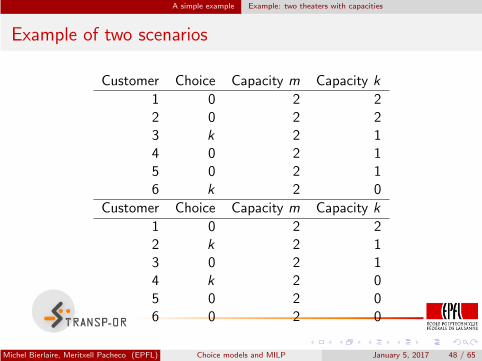
Example of two scenarios
Customer Choice Capacity m Capacity k
1 0 2 22 0 2 23 k 2 14 0 2 15 0 2 16 k 2 0
Customer Choice Capacity m Capacity k
1 0 2 22 k 2 13 0 2 14 k 2 05 0 2 06 0 2 0
Michel Bierlaire, Meritxell Pacheco (EPFL) Choice models and MILP January 5, 2017 48 / 65

Parking management
Outline
1 Demand and supply
2 Disaggregate demand models
3 Choice-based optimizationApplications
4 A generic framework
5 A simple exampleExample: one theaterExample: two theatersExample: two theaters with capacities
6 Parking management7 Conclusion
Michel Bierlaire, Meritxell Pacheco (EPFL) Choice models and MILP January 5, 2017 49 / 65
Parking management
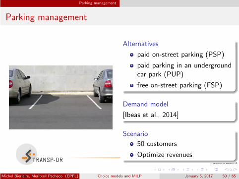
Parking management
Alternatives
paid on-street parking (PSP)
paid parking in an undergroundcar park (PUP)
free on-street parking (FSP)
Demand model
[Ibeas et al., 2014]
Scenario
50 customers
Optimize revenues
Michel Bierlaire, Meritxell Pacheco (EPFL) Choice models and MILP January 5, 2017 50 / 65
Parking management
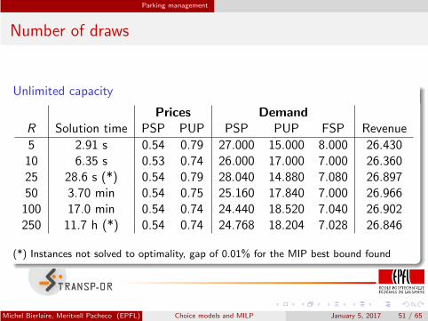
Number of draws
Unlimited capacity
Prices Demand
R Solution time PSP PUP PSP PUP FSP Revenue
5 2.91 s 0.54 0.79 27.000 15.000 8.000 26.43010 6.35 s 0.53 0.74 26.000 17.000 7.000 26.36025 28.6 s (*) 0.54 0.79 28.040 14.880 7.080 26.89750 3.70 min 0.54 0.75 25.160 17.840 7.000 26.966100 17.0 min 0.54 0.74 24.440 18.520 7.040 26.902250 11.7 h (*) 0.54 0.74 24.768 18.204 7.028 26.846
(*) Instances not solved to optimality, gap of 0.01% for the MIP best bound found
Michel Bierlaire, Meritxell Pacheco (EPFL) Choice models and MILP January 5, 2017 51 / 65

Parking management
Number of draws
Capacity of PSP and PUP: 20
Prices Demand
R Solution time PSP PUP PSP PUP FSP Revenue
5 14.95 s 0.63 0.84 18.200 17.200 14.600 25.91410 96.45s 0.57 0.78 19.900 17.900 12.200 25.30525 15.9 min (*) 0.59 0.80 19.480 18.080 12.440 25.95750 2.76 h 0.59 0.80 19.540 18.200 12.260 26.089100 8.31 h (*) 0.59 0.79 19.130 18.660 12.210 26.028250 6.94 days 0.60 0.80 19.044 18.128 12.828 25.929
(*) Instances not solved to optimality, gap of 0.01% for the MIP best bound found
Michel Bierlaire, Meritxell Pacheco (EPFL) Choice models and MILP January 5, 2017 52 / 65
Parking management
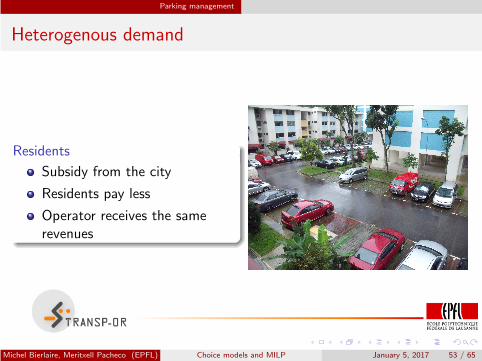
Heterogenous demand
Residents
Subsidy from the city
Residents pay less
Operator receives the samerevenues
Michel Bierlaire, Meritxell Pacheco (EPFL) Choice models and MILP January 5, 2017 53 / 65

Parking management
Subsidy
Prices res Demand res Prices non res Demand non res
Subsidy (%) PSP PUP PSP PUP FSP PSP PUP PSP PUP FSP Revenue20 0.54 0.77 11.8 9.40 5.78 0.68 0.92 7.46 8.60 6.94 29.725 0.54 0.77 12.2 10.2 4.64 0.68 0.92 7.34 8.72 6.94 30.730 0.50 0.67 12.7 10.4 3.86 0.72 0.96 6.16 8.50 8.34 31.840 0.48 0.65 13.7 10.7 2.6 0.80 1.08 4.88 7.20 10.9 34.250 0.46 0.64 15.0 10.4 1.62 0.92 1.28 3.74 5.32 13.94 37.3
Michel Bierlaire, Meritxell Pacheco (EPFL) Choice models and MILP January 5, 2017 54 / 65

Conclusion
Outline
1 Demand and supply
2 Disaggregate demand models
3 Choice-based optimizationApplications
4 A generic framework
5 A simple exampleExample: one theaterExample: two theatersExample: two theaters with capacities
6 Parking management7 Conclusion
Michel Bierlaire, Meritxell Pacheco (EPFL) Choice models and MILP January 5, 2017 55 / 65
Conclusion
Summary
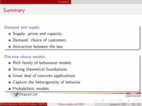
Demand and supply
Supply: prices and capacity
Demand: choice of customers
Interaction between the two
Discrete choice models
Rich family of behavioral models
Strong theoretical foundations
Great deal of concrete applications
Capture the heterogeneity of behavior
Probabilistic models
Michel Bierlaire, Meritxell Pacheco (EPFL) Choice models and MILP January 5, 2017 56 / 65
Conclusion
Optimization
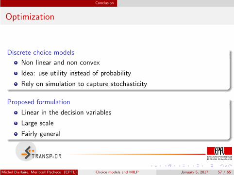
Discrete choice models
Non linear and non convex
Idea: use utility instead of probability
Rely on simulation to capture stochasticity
Proposed formulation
Linear in the decision variables
Large scale
Fairly general
Michel Bierlaire, Meritxell Pacheco (EPFL) Choice models and MILP January 5, 2017 57 / 65
Conclusion
Ongoing research
Decomposition methods
Scenarios are (almost) independent from each other (except objectivefunction)
Individuals are also loosely coupled (except for capacity constraints)
Michel Bierlaire, Meritxell Pacheco (EPFL) Choice models and MILP January 5, 2017 58 / 65
Conclusion
Thank you!
Michel Bierlaire, Meritxell Pacheco (EPFL) Choice models and MILP January 5, 2017 59 / 65

Conclusion
Bibliography I
Andersson, S.-E. (1998).Passenger choice analysis for seat capacity control: A pilot project inscandinavian airlines.International Transactions in Operational Research, 5(6):471–486.
Azadeh, S. S., Marcotte, P., and Savard, G. (2015).A non-parametric approach to demand forecasting in revenuemanagement.Computers & Operations Research, 63:23–31.
Bekhor, S. and Prashker, J. (2001).Stochastic user equilibrium formulation for generalized nested logitmodel.Transportation Research Record: Journal of the Transportation
Research Board, (1752):84–90.
Michel Bierlaire, Meritxell Pacheco (EPFL) Choice models and MILP January 5, 2017 60 / 65

Conclusion
Bibliography II
Benati, S. (1999).The maximum capture problem with heterogeneous customers.Computers & operations research, 26(14):1351–1367.
Bierlaire, M. and Azadeh, S. S. (2016).Demand-based discrete optimization.Technical Report 160209, Transport and Mobility Laboratory, EcolePolytechnique Federale de Lausanne.
Daganzo, C. F. and Sheffi, Y. (1977).On stochastic models of traffic assignment.Transportation science, 11(3):253–274.
Michel Bierlaire, Meritxell Pacheco (EPFL) Choice models and MILP January 5, 2017 61 / 65
Conclusion
Bibliography III
Dial, R. B. (1971).A probabilistic multipath traffic assignment model which obviates pathenumeration.Transportation research, 5(2):83–111.
Fisk, C. (1980).Some developments in equilibrium traffic assignment.Transportation Research Part B: Methodological, 14(3):243–255.
Gilbert, F., Marcotte, P., and Savard, G. (2014a).Logit network pricing.Computers & Operations Research, 41:291–298.
Gilbert, F., Marcotte, P., and Savard, G. (2014b).Mixed-logit network pricing.Computational Optimization and Applications, 57(1):105–127.
Michel Bierlaire, Meritxell Pacheco (EPFL) Choice models and MILP January 5, 2017 62 / 65

Conclusion
Bibliography IV
Haase, K. and Muller, S. (2013).Management of school locations allowing for free school choice.Omega, 41(5):847–855.
Hakimi, S. L. (1990).Locations with spatial interactions: competitive locations and games.Discrete location theory, pages 439–478.
Ibeas, A., dell’Olio, L., Bordagaray, M., and de D. Ortuzar, J. (2014).Modelling parking choices considering user heterogeneity.Transportation Research Part A: Policy and Practice, 70:41 – 49.
Labbe, M., Marcotte, P., and Savard, G. (1998).A bilevel model of taxation and its application to optimal highwaypricing.Management science, 44(12-part-1):1608–1622.
Michel Bierlaire, Meritxell Pacheco (EPFL) Choice models and MILP January 5, 2017 63 / 65
Conclusion
Bibliography V
Marianov, V., Rıos, M., and Icaza, M. J. (2008).Facility location for market capture when users rank facilities byshorter travel and waiting times.European Journal of Operational Research, 191(1):32–44.
Pacheco, M., Azadeh, S. S., and Bierlaire, M. (2016).A new mathematical representation of demand using choice-basedoptimization method.In Proceedings of the 16th Swiss Transport Research Conference,Ascona, Switzerland.
Serra, D. and Colome, R. (2001).Consumer choice and optimal locations models: formulations andheuristics.Papers in Regional Science, 80(4):439–464.
Michel Bierlaire, Meritxell Pacheco (EPFL) Choice models and MILP January 5, 2017 64 / 65
Conclusion
Bibliography VI
Talluri, K. and Van Ryzin, G. (2004).Revenue management under a general discrete choice model ofconsumer behavior.Management Science, 50(1):15–33.
Michel Bierlaire, Meritxell Pacheco (EPFL) Choice models and MILP January 5, 2017 65 / 65