using public land survey (pls) records for...

1

John C. Almendinger April 2009

Revised June 2010 Using Public Land Survey (PLS) Records for Silvicultural Interpretation Background The Public Land Survey bearing-tree database (Almendinger 1996) provides a geographically explicit record of trees before widespread logging and clearing of land in Minnesota. The survey included notes intended to facilitate the sale of federal lands to the private sector. In essence, the notes were the advertisement of land potential to wealthy, eastern investors who had never seen the American west. The notes are of interest to foresters because they describe the natural landscape and resources, particularly timber. In Minnesota, PLS records provide reliable data on the pre-European forests circa 1847-1908, enabling researchers to:

1. make maps of pre-settlement vegetation and forest types (Marshner 1974) 2. make maps of historic tree distributions (Smith 2008) 3. develop ecological land classifications (Hanson 2002) 4. reconstruct natural disturbance patterns and fire history (Grimm 1984) 5. understand lasting impacts of logging (Friedman, S.K., and P.B. Reich. 2005) 6. examine forest pattern and scale (Friedman, S.K., P.B. Reich, and L.E. Frelich. 2001) 7. quantify long-term vegetation changes and identify promising locations for restoration (Galatowitsch

1990) Data Although the PLS was not designed to survey forest vegetation, trees were nonetheless used to document the section and quarter-section corners for the purpose of relocating corners upon sale of the land. At each survey corner the surveyors marked the corner with a charred stake, a large stone, or a pit as a permanent monument. From the corner monument the surveyors selected 1-4 trees to “witness” the corner by recording their:

1. common name (usually to species, sometimes just genus) 2. distance from the corner 3. azimuth or “bearing” from the corner 4. diameter in inches

North Section 5 Section 4 5” tamarack 4” spruce 13 links 23 links 6” tamarack 40 links 5” birch 32 links Section 8 Section 9

On left: A section of survey notes for the bearing trees used to reference the corner common to sections 4,5,8 and 9. The notes indicate also that a wooden post was used to monument the corner and it was notched to indicate the number of miles to the south and east township boundaries. On right: A cartoon plan-view showing approximate tree positions (circles) relative to the corner (diamond).

Common name, distance, azimuth, and diameter are the fundamental tree data available for quantitative analyses.

2

At section corners the surveyors were instructed to select 4 witness trees; at quarter-section corners they were to select just two. No two witness trees were to fall in the same quadrant assuring that they fell uniquely into sections, the numbers of which were scribed on the witness tree along with their township and range numbers. In a standard township there are 108 total corners: 36 section corners yielding 144 tree records and 72 quarter section corners yielding also 144 trees. Our convention for creating GIS covers of bearing trees is to record for each township the east and north boundary corners, but not those on the west or south (right). This is done so that a mosaic of township covers will not have duplicate records.

The survey notes also provide an account of “features” encountered while running mile-long segments between section corners (right). These are the so called “line notes” and the features mentioned most often were bodies of water and obvious changes in vegetation such as swamps, marsh, prairie, etc. Especially important to foresters is consistent mention of damage to the timber resource by fire or windthrow. The field notes include the explicit point along the line where there were changes in these features such as: “shore of Mud Lake,” “leave timber and enter prairie,” left bank of small brook,” etc. These line notes allow for the construction of a map consisting of section-line segments with vegetation or disturbance attributes. At the time of the survey, General Land Office (GLO) clerks prepared township plats from the line notes. Today, GIS covers can be prepared to help with resource assessment and mapping.

Above: A set of line notes for surveying a mile of line going east between sections 5 and section 32 (north township boundary). Along this line the surveyor started in a swamp and then encountered a small lake, then upland [forest], then a marsh, then upland [forest] with a rock ledge. The left column shows the distances in chains from the starting corner to the boundaries between these features and the quarter-section (40ch) and section corner (80ch).

The PLS notes provide a sparse, but systematic survey of the forest vegetation on a half-mile grid and yielding about 288 tree records per township. Across the state, there are 249,466 section and quarter-section corners that document the occurrence of 352,896 bearing trees.

The PLS line notes help us to model the likely NPC class of a survey corner for the purpose of quantitatively calculating disturbance regimes and developing models of succession associated with an NPC. These notes also allow for the construction of general maps of the historic vegetation.

Above: Schematic showing the pattern of bearing trees (green) as they occur at section (black) and quarter-section (gray) corners in a township.

3

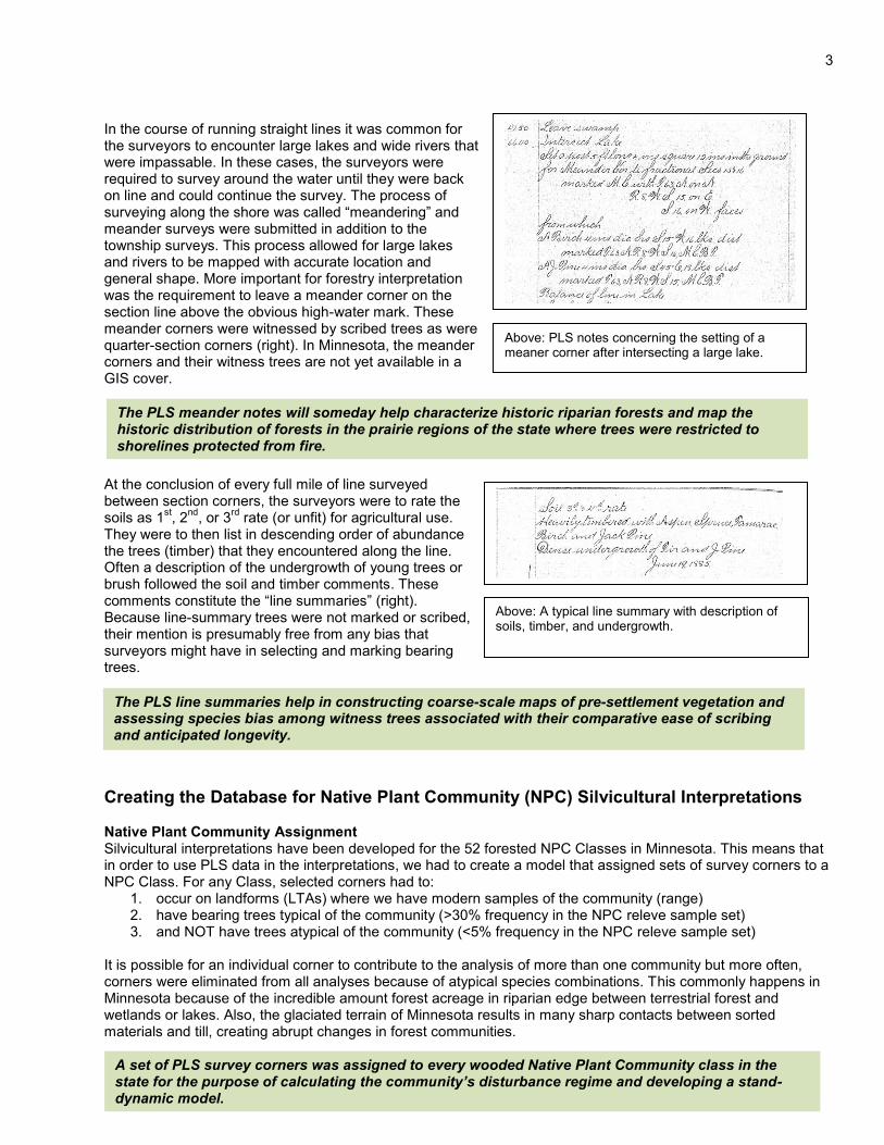
In the course of running straight lines it was common for the surveyors to encounter large lakes and wide rivers that were impassable. In these cases, the surveyors were required to survey around the water until they were back on line and could continue the survey. The process of surveying along the shore was called “meandering” and meander surveys were submitted in addition to the township surveys. This process allowed for large lakes and rivers to be mapped with accurate location and general shape. More important for forestry interpretation was the requirement to leave a meander corner on the section line above the obvious high-water mark. These meander corners were witnessed by scribed trees as were quarter-section corners (right). In Minnesota, the meander corners and their witness trees are not yet available in a GIS cover.

At the conclusion of every full mile of line surveyed between section corners, the surveyors were to rate the soils as 1st, 2nd, or 3rd rate (or unfit) for agricultural use. They were to then list in descending order of abundance the trees (timber) that they encountered along the line. Often a description of the undergrowth of young trees or brush followed the soil and timber comments. These comments constitute the “line summaries” (right). Because line-summary trees were not marked or scribed, their mention is presumably free from any bias that surveyors might have in selecting and marking bearing trees.

Creating the Database for Native Plant Community (NPC) Silvicultural Interpretations Native Plant Community Assignment Silvicultural interpretations have been developed for the 52 forested NPC Classes in Minnesota. This means that in order to use PLS data in the interpretations, we had to create a model that assigned sets of survey corners to a NPC Class. For any Class, selected corners had to:

1. occur on landforms (LTAs) where we have modern samples of the community (range) 2. have bearing trees typical of the community (>30% frequency in the NPC releve sample set) 3. and NOT have trees atypical of the community (<5% frequency in the NPC releve sample set)

It is possible for an individual corner to contribute to the analysis of more than one community but more often, corners were eliminated from all analyses because of atypical species combinations. This commonly happens in Minnesota because of the incredible amount forest acreage in riparian edge between terrestrial forest and wetlands or lakes. Also, the glaciated terrain of Minnesota results in many sharp contacts between sorted materials and till, creating abrupt changes in forest communities.

Above: PLS notes concerning the setting of a meaner corner after intersecting a large lake.

Above: A typical line summary with description of soils, timber, and undergrowth.

The PLS meander notes will someday help characterize historic riparian forests and map the historic distribution of forests in the prairie regions of the state where trees were restricted to shorelines protected from fire.

The PLS line summaries help in constructing coarse-scale maps of pre-settlement vegetation and assessing species bias among witness trees associated with their comparative ease of scribing and anticipated longevity.

A set of PLS survey corners was assigned to every wooded Native Plant Community class in the state for the purpose of calculating the community’s disturbance regime and developing a stand-dynamic model.

4

Assignment of Generic or Ambiguous Taxa A constant problem in analyzing PLS data are generic references to “oak,” “maple,” or “pine.” For this analysis, the species with the greatest frequency in the releve samples of the NPC was awarded with the generic or ambiguous references. For example, pin, red, black, bur, and white oak all occur in the FDs27 community, but pin oak has the greatest frequency so all “oak” bearing trees at corners assigned to FDs27 were tallied as pin oak. In other cases the reference may be ambiguous depending upon how much the tree ranges overlap. For example, “Black oak” clearly refers to either red or black oak in the survey notes but for corners assigned to the MHc26 community all references of “black oak” were tallied a red oak, because the community is outside of the range of black oak. Natural Disturbance Regimes Understanding natural disturbance regimes is prerequisite for designing silvicultural systems and treatments that emulate natural processes. Theoretically, “natural” treatments favor trees adapted to the site, conserve local gene pools by relying on natural regeneration, maintain native plants in the understory, are less risky than agricultural approaches, and cheaper to implement. Because clear-cutting and other stand-regenerating systems are so often employed, it is important to determine which NPCs were maintained by stand-replacing disturbances and, further, to estimate the natural rotation. For many NPCs the natural rotation far exceeds commercial rotation, and this requires us to look to other silvicultural strategies for harvest and regeneration. Thus, we must also estimate the frequency and intensity of disturbances that maintain these kinds of forest communities.

The surveyors explicitly described burned and windthrown land when working within the forested regions of Minnesota. When in the prairie region and especially along the prairie/forest border, the surveyors used a variety of terms to describe wooded vegetation understood to be maintained by frequent disturbance. Most often this was fire, but in some regions wind was important as well. Thus, geographic context is an important consideration when trying to determine if a surveyor’s comments are indicating that the corner was 1) undisturbed, 2) catastrophically disturbed, or 3) recently affected by a less intense, maintenance disturbance. Placing corners in these three categories is the critical step that allows the calculation of disturbance regimes. To get at this, we must understand the surveyor’s physiognomic descriptions of the vegetation at the corners: prairie, grove, bottoms, barrens, burned lands, windthrown timber, etc.

Stocking (i.e., tree density) is the most important element of their physiognomic descriptions. Our initial step in the analysis was to understand how the distances to bearing trees affected the surveyor’s vocabulary. For all of the types, we calculated the mean distance to bearing trees which allowed us to rank and group the types in some sensible fashion.

Table 1. Vegetation types mentioned by surveyors and their mean distances in links to their bearing trees. Columns roughly ranked by range of distances. (NOTA means “no other tree around.”)

Wooded types Disturbance types Riverine types Fire maintained types Open types Swamp 40 Windthrow 72 Bottomland 135 Thicket 92 Meadow 183 Forest 50 Burned land 76 Dry land 157 Pine openings 113 NOTA 192

Dry ridge 60 Oak openings 145 Prairie 236 Grove 69 Scattering oak 166 Marsh 278 Island 70 Barrens 177 Wet prairie 411

The goal of our disturbance analysis was to estimate the rotation of stand-replacement and maintenance disturbances unique to each NPC class.

Our rules for assessing disturbance at survey corners were individually set for each physiognomic vegetation type across the state.

5

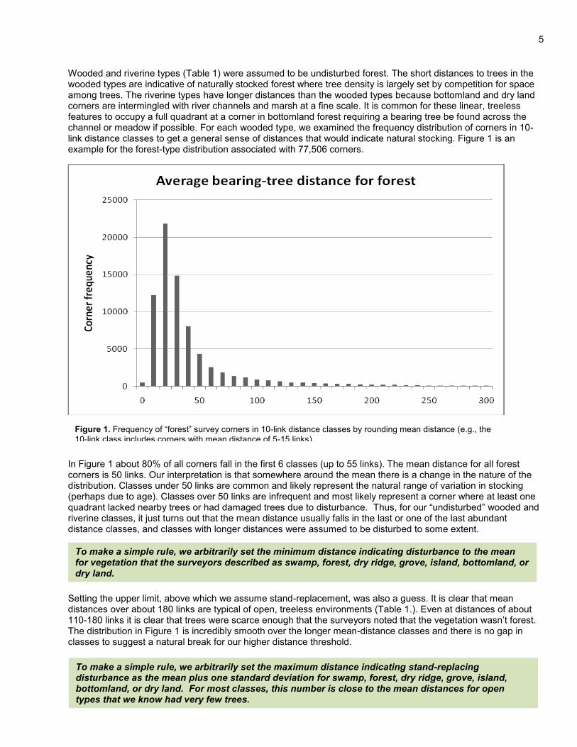
Wooded and riverine types (Table 1) were assumed to be undisturbed forest. The short distances to trees in the wooded types are indicative of naturally stocked forest where tree density is largely set by competition for space among trees. The riverine types have longer distances than the wooded types because bottomland and dry land corners are intermingled with river channels and marsh at a fine scale. It is common for these linear, treeless features to occupy a full quadrant at a corner in bottomland forest requiring a bearing tree be found across the channel or meadow if possible. For each wooded type, we examined the frequency distribution of corners in 10-link distance classes to get a general sense of distances that would indicate natural stocking. Figure 1 is an example for the forest-type distribution associated with 77,506 corners.

In Figure 1 about 80% of all corners fall in the first 6 classes (up to 55 links). The mean distance for all forest corners is 50 links. Our interpretation is that somewhere around the mean there is a change in the nature of the distribution. Classes under 50 links are common and likely represent the natural range of variation in stocking (perhaps due to age). Classes over 50 links are infrequent and most likely represent a corner where at least one quadrant lacked nearby trees or had damaged trees due to disturbance. Thus, for our “undisturbed” wooded and riverine classes, it just turns out that the mean distance usually falls in the last or one of the last abundant distance classes, and classes with longer distances were assumed to be disturbed to some extent.

Setting the upper limit, above which we assume stand-replacement, was also a guess. It is clear that mean distances over about 180 links are typical of open, treeless environments (Table 1.). Even at distances of about 110-180 links it is clear that trees were scarce enough that the surveyors noted that the vegetation wasn’t forest. The distribution in Figure 1 is incredibly smooth over the longer mean-distance classes and there is no gap in classes to suggest a natural break for our higher distance threshold.

Figure 1. Frequency of “forest” survey corners in 10-link distance classes by rounding mean distance (e.g., the 10-link class includes corners with mean distance of 5-15 links).

To make a simple rule, we arbitrarily set the minimum distance indicating disturbance to the mean for vegetation that the surveyors described as swamp, forest, dry ridge, grove, island, bottomland, or dry land.

To make a simple rule, we arbitrarily set the maximum distance indicating stand-replacing disturbance as the mean plus one standard deviation for swamp, forest, dry ridge, grove, island, bottomland, or dry land. For most classes, this number is close to the mean distances for open types that we know had very few trees.

6

The frequency distributions of fire-maintained types are different from the wooded and riverine types. At distances greater than the peak class, the fall in frequency is nearly linear, an example of which is for oak openings (Figure 2.). There is no obvious point of inflection to set the lower, naturally-stocked, undisturbed limit, nor are there breaks in the distribution that can help us set the upper limit for catastrophic disturbance. It is important to remember that we are interpreting the use of terms like “openings” and “scatterings” to corners that we believe from modern vegetation to be capable of forest stocking. Almost certainly, these terms were used to describe recent disturbance that caused trees to be sparser than normal “forest.” To help us interpret the use of these terms to describe forest, we returned to the coarser analysis. Corners with distances under 50 links were almost certainly in places one would describe as undisturbed forest. Corners with distances over 200 links were in places where tree density was low and comparable to open habitats like prairie and meadow.

In addition to distance, we found it important to consider also missing bearing trees as evidence of disturbance. A common survey note is “NOTA” meaning “no other tree around,” which was the surveyor’s explanation for not marking all of the required bearing trees (i.e., 4 at section corners and 2 at quarter-section corners). Most often this note appeared at corners described as one of the fire-maintained or open community groups (Table 1.). NOTA was also used at corners described as burned or windthrown. Within the context of interpreting corners modeled as forest or woodland, NOTA almost certainly was relating to some kind of disturbance that left dead trees or trees too small to scribe. Table 2 describes our model for assigning a disturbance class based on both distance and complement of bearing trees.

Figure 2. Frequency of “oak opening” survey corners in 10-link distance classes by rounding mean distance (e.g., the 10-link class includes corners with mean distance of 5-15 links).

To make a simple rule for corners described as thicket, pine openings, oak openings, scattering timber, and barrens, we arbitrarily set the minimum distance indicating disturbance to 50 links, and we set the maximum distance indicating stand-replacing disturbance at 200 links.

7

Adjusting the Model – Window of Recognition It is obvious that several pragmatic decisions and rules were made in order to assign corners to disturbance categories. Even if these rules are reasonable, one must still set a “window of recognition” in order to make quantitative estimates of stand-replacing and maintenance rotations. The window of recognition is the span of years for which a surveyor would have bothered to describe a disturbance. Would a surveyor recognize and care to report that a stand had been burned 5, 10, 15, or 20 years after the fact? We believe that mention of fire and windthrow was more an excuse for not marking bearing trees than any conscientious effort to alert potential buyers to fire- or wind-damaged timber. Consider the fact that quaking aspen is the early successional species for nearly all terrestrial forests in Minnesota. The surveyors actually marked and scribed some 390, 2-inch aspen bearing trees and some 3,039 three-inch trees. Clearly, surveyors would bother to scribe 2-3” trees if that was their only choice. Our age/diameter models for 2-3” aspen trees suggest that these trees were between 11 and 18 years old respectively. If commenting about fire and wind was an excuse, then the window of recognition should be somewhere in the 11-18 year range because that is when trees reach a minimum diameter for marking.

Alternatively, a window of recognition is empirically set to “force” the rotation model to match the estimates from studies using more reliable methods. In the Great Lakes States, there are reconstructions of disturbance regimes from fire-scar studies (Frissell 1973), stand-origin mapping (Heinselman 1996), and charcoal analysis of varved sediments (Clark 1988). When we model disturbance regimes from bearing trees in these same regions, a window of 15 years tends to yield results similar to the other methods for stand-replacing disturbance.

Many detailed investigations of forest disturbance do not calculate rotations of maintenance disturbance, but recognize its confounding effect on estimating stand-replacing events. Trees with multiple fire-scars attest that some forest types are affected more by maintenance surface fire than catastrophic crown fires. Dendrochronological reconstructions of stand history also attest that maintenance events (fire and non-fire) are common and important, releasing cohorts of advance regeneration and providing some growing space in the canopy (e.g. Bergeron et al. 2002). Minor peaks in varve charcoal are also more common than major ones, possibly recording maintenance fires. Calculating maintenance disturbance is more complicated than stand-replacement because the signal is weaker, reliable studies are fewer, and the cause less obvious. However, some estimate is absolutely required to provide guidance in applying intermediate silvicultural treatments to the right NPCs. As was the case for estimating stand-replacing rotations, adjusting the window of recognition is the easiest way to adjust the model. Logic would suggest that the window should be shorter for maintenance events because the disturbance is less intense and evidence of it might be gone in 15 years. If the surveyors really used terms like burned or windthrown to explain the lack of bearing trees, it is likely that they did so less often on lands lightly disturbed because there were trees around – they just had to go a little farther to find bearing trees and might not always find a suitable tree in all quadrants. We found that a 5-year window produced rotations that matched what one might guess from multiple-scarred trees. Also, the ratio of maintenance events to catastrophic ones seemed within the range of what one might expect from the ratio of strong charcoal peaks to minor ones in varve studies.

Table 2. Rules for assigning a disturbance class to survey corners not explicitly described as burned or windthrown. Assumed undisturbed – Wooded and Riverine groups < mean between mean and mean + SD >Mean + SD

Full complement Undisturbed Undisturbed Maintenance Partial complement Undisturbed Maintenance Burned

Assumed disturbed – Fire-maintained group < 50 links 50-206 links > 206 links

Full complement Undisturbed Maintenance Burned Partial complement Maintenance Maintenance Burned

Within their type, survey corners were assigned their final disturbance class – undisturbed, partially disturbed, catastrophically disturbed – by a combination of the corner’s mean distance to its bearing trees and whether it had its full complement of 2 or 4 bearing trees.

We used a 15-year window of recognition because it yields rotations comparable to rotations calculated from fire-scars, stand-origin maps, and varved lake sediments.

A 5-year recognition window was used to calculate maintenance rotations because it seems to fit fire-scar and varve studies.

8

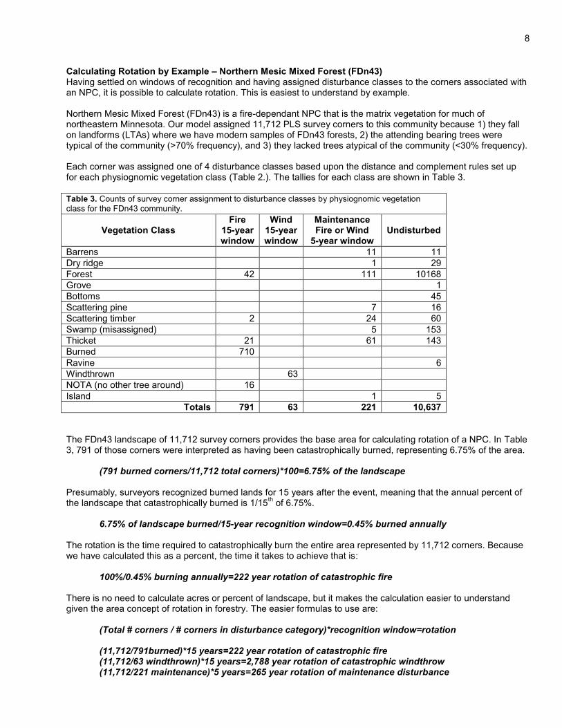
Calculating Rotation by Example – Northern Mesic Mixed Forest (FDn43) Having settled on windows of recognition and having assigned disturbance classes to the corners associated with an NPC, it is possible to calculate rotation. This is easiest to understand by example. Northern Mesic Mixed Forest (FDn43) is a fire-dependant NPC that is the matrix vegetation for much of northeastern Minnesota. Our model assigned 11,712 PLS survey corners to this community because 1) they fall on landforms (LTAs) where we have modern samples of FDn43 forests, 2) the attending bearing trees were typical of the community (>70% frequency), and 3) they lacked trees atypical of the community (<30% frequency). Each corner was assigned one of 4 disturbance classes based upon the distance and complement rules set up for each physiognomic vegetation class (Table 2.). The tallies for each class are shown in Table 3. Table 3. Counts of survey corner assignment to disturbance classes by physiognomic vegetation class for the FDn43 community.

Vegetation Class Fire

15-year window

Wind 15-year window

Maintenance Fire or Wind

5-year window Undisturbed

Barrens 11 11 Dry ridge 1 29 Forest 42 111 10168 Grove 1 Bottoms 45 Scattering pine 7 16 Scattering timber 2 24 60 Swamp (misassigned) 5 153 Thicket 21 61 143 Burned 710 Ravine 6 Windthrown 63 NOTA (no other tree around) 16 Island 1 5

Totals 791 63 221 10,637 The FDn43 landscape of 11,712 survey corners provides the base area for calculating rotation of a NPC. In Table 3, 791 of those corners were interpreted as having been catastrophically burned, representing 6.75% of the area.

(791 burned corners/11,712 total corners)*100=6.75% of the landscape Presumably, surveyors recognized burned lands for 15 years after the event, meaning that the annual percent of the landscape that catastrophically burned is 1/15th of 6.75%.

6.75% of landscape burned/15-year recognition window=0.45% burned annually The rotation is the time required to catastrophically burn the entire area represented by 11,712 corners. Because we have calculated this as a percent, the time it takes to achieve that is:

100%/0.45% burning annually=222 year rotation of catastrophic fire There is no need to calculate acres or percent of landscape, but it makes the calculation easier to understand given the area concept of rotation in forestry. The easier formulas to use are:

(Total # corners / # corners in disturbance category)*recognition window=rotation

(11,712/791burned)*15 years=222 year rotation of catastrophic fire (11,712/63 windthrown)*15 years=2,788 year rotation of catastrophic windthrow (11,712/221 maintenance)*5 years=265 year rotation of maintenance disturbance

9

It is also useful to calculate the rotation of all fire (or wind), regardless if it was catastrophic or maintenance. To make this calculation it is easiest to sum the annual percents.

0.45% burned catastrophically each year 0.37% burned in maintenance event 0.45%+0.37%=0.82% annual=122 year rotation for all types of fires

It is the rotation of all fires that tends to reasonably match the published estimates of return intervals. For example, in the BWCAW Heinselman (1996) reports return intervals for the common forest types: Aspen-Birch-Conifer (70-110 years), Red Pine (<100), and White Pine (>100). These cover types, especially the white pine, are predominantly the FDn43 community for which we calculate a 122 year rotation for all fires. Across the state in Itasca State Park, Frissell (1973) reports a return interval of 22 years in what is mostly FDc34 forest. Our FDc34 calculation for all fires is a comparable 23 years, derived from an estimate of stand-regenerating rotation at 113 years and a 30-year rotation for maintenance fire. Also in Itasca State Park, Clark’s investigation of charcoal in the varved sediments of Deming Lake shows that nearly all fire-scars on trees within the lake’s catchment can be matched to charcoal peaks (Clark 1988), but there are usually some charcoal peaks without corroborating fire-scars. Thus, charcoal peaks are more frequent than fire-scars, suggesting a shorter return interval of all fires, probably in the range of 10-15 years. Stand Dynamics Understanding natural stand dynamics is the essence of prescription writing. Without some understanding of how dynamics affect tree establishment, thinning, recruitment, competitive ability, form, longevity, and succession during “unsupervised” stand maturation – foresters cannot write worthwhile prescriptions. For the most part, prescriptions are written to alter, accelerate, or allow the natural course of events in a forest in order to meet a management objective. PLS data are not inherently temporal. To create a model of stand dynamics we must somehow rank survey corners in a way that is reflective of time. We did this by calculating tree age from diameter. For each species, we used FIA site-index trees to create quadratic equations that model the age/diameter relationship.

Age=C+A*dbh+B*dbh2 (where C is a constant, A&B are coefficients from FIA model)

However, tree ages are not stand age, which is what we would like to know for each corner. The best that can be done is to assign each corner a stand-age equal to the age of the oldest bearing tree at that corner. Presumably, this is a minimum estimate of how long the stand has avoided a catastrophic disturbance. This is NOT true stand age because no corner can be assigned an age beyond the biological longevity of its old-growth species. However, this does reasonably rank corners with smaller-diameter/younger trees for the first 100 years or so. We believe that this is good enough to make some broad interpretations about stand dynamics and tree recruitment throughout the early years of stand maturation.

Corners were then placed into 10-year age classes with the exception of the initial 15-year class that matches the 15-year disturbance “recognition window” used to calculate the rotations of fire and windthrow. Small diameter (<4”) bearing trees were “forced” into age class 0-15 when they occurred at corners described as burned or windthrown. Otherwise, corners were assigned to age classes when the diameter of the oldest tree would lead us to believe that it was between 15-25 years old, 25-35 years old, etc. Thus, age-class 10 includes trees at survey corners where the oldest tree was estimated to be between 0 and 15 years old; age-class 20 holds trees at survey corners where the oldest tree was estimated to be between 15 and 25 years old, etc. The reason for doing this was to calculate for each class, the relative abundance of the component species. Relative abundance is the percentage of all trees in an age-class that are a particular species.

Bearing tree ages were estimated from their diameters by using a quadratic equation that was fit to FIA site-index trees.

Survey corners were assigned “stand ages” equal to that of the age of the oldest, large-diameter tree at the corner.

Survey corners were collected into 10-year age-classes to calculate the relative abundance of species.

10

Example Data-matrix for FDn43

Frequency

Col Pct 10.0000 30.0000 50.0000 70.0000 90.0000 110.0000 130.0000 150.0000 170.0000 190.0000 200.0000 300.0000 Total

AS 79 1836 1650 828 250 241 115 89 39 27 129 4 5287

67.52 55.14 17.36 14.93 9.27 8.46 6.18 7.91 5.36 4.79 7.37 3.39

BA 0 0 6 1 4 0 1 0 0 0 0 0 12

0.00 0.00 0.06 0.02 0.15 0.00 0.05 0.00 0.00 0.00 0.00 0.00

BE 0 0 0 2 0 0 0 0 0 0 0 0 2

0.00 0.00 0.00 0.04 0.00 0.00 0.00 0.00 0.00 0.00 0.00 0.00

BG 0 8 17 5 8 1 1 1 0 0 0 0 41

0.00 0.24 0.18 0.09 0.30 0.04 0.05 0.09 0.00 0.00 0.00 0.00

BO 0 0 2 2 0 1 0 0 1 0 0 1 7

0.00 0.00 0.02 0.04 0.00 0.04 0.00 0.00 0.14 0.00 0.00 0.85

CH 0 0 3 0 1 0 0 0 0 0 0 0 4

0.00 0.00 0.03 0.00 0.04 0.00 0.00 0.00 0.00 0.00 0.00 0.00

CO 0 0 1 0 0 1 0 0 0 0 0 0 2

0.00 0.00 0.01 0.00 0.00 0.04 0.00 0.00 0.00 0.00 0.00 0.00

EL 0 3 9 6 0 1 2 0 2 0 0 0 23

0.00 0.09 0.09 0.11 0.00 0.04 0.11 0.00 0.28 0.00 0.00 0.00

FI 0 97 2225 587 230 309 269 160 66 84 213 11 4251

0.00 2.91 23.40 10.58 8.52 10.84 14.45 14.22 9.08 14.89 12.17 9.32

GA 0 5 16 2 1 2 0 1 0 1 0 0 28

0.00 0.15 0.17 0.04 0.04 0.07 0.00 0.09 0.00 0.18 0.00 0.00

IR 0 0 0 0 1 0 0 0 0 0 0 0 1

0.00 0.00 0.00 0.00 0.04 0.00 0.00 0.00 0.00 0.00 0.00 0.00

JP 21 407 563 246 49 150 48 91 16 47 91 0 1729

17.95 12.22 5.92 4.43 1.82 5.26 2.58 8.09 2.20 8.33 5.20 0.00

LI 0 0 4 2 1 0 0 1 0 0 1 0 9

0.00 0.00 0.04 0.04 0.04 0.00 0.00 0.09 0.00 0.00 0.06 0.00

MH 0 0 1 0 0 0 0 0 0 0 0 0 1

0.00 0.00 0.01 0.00 0.00 0.00 0.00 0.00 0.00 0.00 0.00 0.00

RM 0 4 123 62 32 8 8 4 14 1 7 1 264

0.00 0.12 1.29 1.12 1.19 0.28 0.43 0.36 1.93 0.18 0.40 0.85

RO 0 3 3 6 4 3 2 1 1 0 1 1 25

0.00 0.09 0.03 0.11 0.15 0.11 0.11 0.09 0.14 0.00 0.06 0.85

RP 6 60 491 495 253 201 120 51 49 13 77 3 1819

5.13 1.80 5.16 8.92 9.38 7.05 6.45 4.53 6.74 2.30 4.40 2.54

SU 0 0 7 10 6 2 2 0 3 1 3 1 35

0.00 0.00 0.07 0.18 0.22 0.07 0.11 0.00 0.41 0.18 0.17 0.85

TA 0 10 32 25 9 22 36 14 35 0 35 1 219

0.00 0.30 0.34 0.45 0.33 0.77 1.93 1.24 4.81 0.00 2.00 0.85

WB 8 795 2325 1910 776 700 368 175 151 100 285 15 7608

6.84 23.87 24.46 34.43 28.76 24.56 19.77 15.56 20.77 17.73 16.29 12.71

WC 0 4 207 87 149 88 60 7 18 4 28 6 658

0.00 0.12 2.18 1.57 5.52 3.09 3.22 0.62 2.48 0.71 1.60 5.08

WI 0 7 1 0 0 0 0 0 0 0 0 0 8

0.00 0.21 0.01 0.00 0.00 0.00 0.00 0.00 0.00 0.00 0.00 0.00

WP 3 79 1576 971 827 371 392 86 273 35 368 69 5050

2.56 2.37 16.58 17.50 30.65 13.02 21.06 7.64 37.55 6.21 21.03 58.47

WS 0 12 245 290 91 749 437 444 59 250 512 5 3094

0.00 0.36 2.58 5.23 3.37 26.28 23.48 39.47 8.12 44.33 29.26 4.24

YB 0 0 0 10 6 0 0 0 0 1 0 0 17

0.00 0.00 0.00 0.18 0.22 0.00 0.00 0.00 0.00 0.18 0.00 0.00

Total 117 3330 9507 5547 2698 2850 1861 1125 727 564 1750 118 30194

Above: An example of the FDn34 model matrix in 20-year age-classes (columns) by species (rows). The matrix cells contain the raw counts of bearing trees above their column percent. Tree codes are AS, aspen; BA, black ash; BE, beech [likely not]; BG, balsam poplar; BO, bur oak; CH, cherry; CO, cottonwood; EL, elm; FI, balsam fir; GA, green ash; IR, ironwood; JP, jack pine; LI, basswood; MH, mountain ash; RM, red maple; RO, red oak; RP, red pine; SU, sugar maple; TA, tamarack; WB, paper birch; WC, white cedar; WI, willow; WP, white pine; WS, white spruce; YB, yellow birch.

11

References Almendinger, J.C. 1996. Minnesota’s Bearing Tree Database. Biological Report No. 56. Minn. Dept. Nat. Res., St.

Paul, MN. Bergeron, Y., B. Denneler, D. Charron, and M-P Girardin. 2002. Using dendrochronology to reconstruct disturbance and forest dynamics around Lake Duparquet, northwestern Quebec. Dendrochronologia 20/1-2 175-189 Clark, J.S. Stratigraphic charcoal analysis on petrographic thin sections: Application to fire history in Northwestern

Minnesota. Quaternary Research 30:81-91. Friedman, S.K., and P.B. Reich. 2005. Regional legacies of logging: Departure from presettlement forest

conditions in northern Minnesota. Ecol. Appl. 15(2):726-744. Friedman, S.K., P.B. Reich, and L.E. Frelich. 2001. Multiple scale composition and spatial distribution patterns of

the north-eastern Minnesota presettlement forest. J. Ecol. 89:538–554. Frissell, S.S Jr. 1973. The importance of fire as a natural ecological factor in Itasca State Park, Minnesota.

Quaternary Research 3:397-407. Galatowitsch, S.M. 1990. Using the original land survey notes to reconstruct presettlement landscapes in the

American West. Great Basin Naturalist 50(2):181-191. Grimm, E.C. 1984. Fire and other factors controlling the Big Woods vegetation in Minnesota in the mid-nineteenth

century. Ecol. Monogr. 54:291-311. Hanson, D.S (2002). Ecological Provinces, Sections, and Subsections of Minnesota. Department of Natural

Resources. St. Paul Minnesota. http://www.dnr.state.mn.us/ecs/index.html. (accessed August 21, 2006 maps and descriptions of province, section, and subsection map unit descriptions)

Heinselman, M.L. 1996. The Boundary Waters Wilderness ecosystem. University of Minnesota Press,

Minneapolis, MN. Marschner, F.J. 1974. The original vegetation of Minnesota (map; scale 1:500,000). USDA For. Serv. North

Central For. Exp. Stn. St. Paul, MN. (redraft of the 1930 edition) Smith, W.R. (2008). Trees and Shrubs of Minnesota. University of Minnesota Press, Minneapolis, MN.

http://www.dnr.state.mn.us/ecs/index.html

12

Standard PLS-derived Tables and Figures for Silviculture and Forest Management Having assembled the basic PLS database, we performed several analyses to address silvicultural interpretation. From these analyses, we have created a standard set of tables and figures for each wooded NPC class. Below is a summary of these standard products, followed by an example of each with an account of methods, purpose, and applications. Table PLS-1, Historic abundance of trees in natural growth-stages, provides a general, tabular model of stand dynamics. Relative abundances of trees by growth-stage (grouping of contiguous age-classes) are the data presented. This table can be used to:

1. Identify initial-cohort species 2. Identify the successional status of the different tree species 3. Recognize impending decline and replacement 4. Assess the balance of growth-stages on the historic landscape for SFRMP 5. Assess data reliability

Figure SUM-1, Historic abundance & recruitment of trees throughout stand maturation, provides a general, graphic depiction of stand dynamics. Relative abundances of all trees and recruiting trees by age-class are the data presented. This figure can be used to:

1. Estimate the timing of a species’ peak abundance to set commercial rotation 2. Identify basic species behavior 3. Allow recruitment of advance regeneration prior to treatment 4. Schedule stand evaluations based upon stand age

Table PLS-3, Historic abundance of trees following disturbance, provides an impression of how important disturbance was to the species characteristic of the NPC class. The raw counts of bearing trees and their relative abundance are presented in the fire, windthrow, maintenance, and undisturbed categories. This table can be used to:

1. Determine the disturbance that was most prevalent and characteristic of the community 2. Estimate which species are likely to respond positively, given a certain disturbance 3. Estimate which disturbance category was most favorable, given a certain species 4. Assess data reliability

Figure PLS-4, Ordination of historic age-classes, presents a graphic view of the rate of succession. Ordination scores for 20-year age-classes are plotted in two dimensions, and interpreted as to their affinity for growth-stages or transitions. This figure was used to:

1. Define periods of stable forest composition known as growth-stages 2. Define periods of transition characterized by mortality and replacement 3. Aid communication of silvicultural ideas by growth-stage

Table PLS-5, Historic windows of recruitment, presents a table that summarizes how well the different species recruit in the open, post-disturbance environment (PD window), under a dense canopy during self-thinning (SSG window), in large canopy gaps (LG window), and in small gaps (SG window).

1. Identify silvicultural systems that would favor recruitment of selected crop species 2. Identify silvicultural treatments that favor recruitment of selected crop species when regen is present. 3. Identify species that might do well when underplanted 4. Schedule inspections to assess advance regeneration and set the timing of treatments that would release advance

regeneration at maximum stocking Table PLS-6, Natural disturbance rotations, presents the estimates of rotation for stand-regenerating fire, stand-regenerating wind, and less severe maintenance events for a community and allied communities for comparison.

1. Understand the geography of disturbance in Minnesota 2. Help create fire-regime maps for planning and fire response 3. Examine the difference between natural and commercial rotation on landscape age-class distributions 4. Match silvicultural systems and treatments to NPC classes to emulate the timing and severity of disturbance.

13

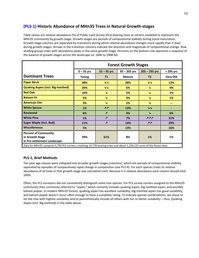
(PLS-1) Historic Abundance of MHn35 Trees in Natural Growth-stages Table values are relative abundance (%) of Public Land Survey (PLS) bearing trees at corners modeled to represent the MHn35 community by growth-stage. Growth-stages are periods of compositional stability during stand maturation. Growth-stage columns are separated by transitions during which relative abundance changes more rapidly than it does during growth-stages. Arrows in the transition columns indicate the direction and magnitude of compositional change. Row shading groups trees with abundance peaks in the same growth-stage. Percents on the bottom row represent a snapshot of the balance of growth-stages across the landscape ca. 1846 to 1908 AD.

Dominant Trees

Forest Growth Stages

0 – 55 yrs 55 – 95 yrs 95 – 205 yrs 205 – 295 yrs > 295 yrs

Young T1 Mature T2 Very Old

Paper Birch 38% 28% 12%

Quaking Aspen (incl. Big-toothed) 20% 6% 4%

Red Oak 10% 5% 1%

Balsam Fir 5% 3% 1%

American Elm 3% 2% --

White Spruce 1% 13% -

Basswood 6% 9% 6%

White Pine 1% 7% 31%

Sugar Maple (incl. Red) 11% 14% 29%

Miscellaneous 5% 13% 16%

Percent of Community in Growth Stage in Pre-settlement Landscape

39% 51% 8% 1% 1%

Data for MHn35 comprise 5,794 PLS corners, involving 14,778 bearing trees and about 1,234,122 acres of the forest class.

PLS-1, Brief Methods

Ten-year age-classes were collapsed into broader growth-stages (columns), which are periods of compositional stability separated by episodes of comparatively rapid change in composition (see PLS-4). For each species (row) its relative abundance of all trees in that growth-stage was calculated (cell). Because it is relative abundance each column should total 100%. Often, the PLS surveyors did not consistently distinguish some tree species. For PLS survey corners assigned to the MHn35 community they commonly referred to “aspen,” which certainly includes quaking aspen, big-toothed aspen, and possibly balsam poplar. In modern MHn35 forests, quaking aspen has excellent suitability; big-toothed aspen has good suitability, and balsam poplar doesn’t occur often enough to have a suitability rating. To indicate species combinations, we chose to list the tree with highest suitability and to parenthetically include all others with fair or better suitability – thus, Quaking Aspen (incl. Big-toothed) in the table above.

14

PLS-1, Silvicultural Applications

1. Identify initial-cohort species a. In general, species with more than about 5% relative abundance in the young growth-stage are

considered to be initial-cohort trees. b. Because of variety in the intensity and type (fire, wind, disease) of stand-regenerating disturbance, most

initial-cohort trees were capable of dominating a young stand. (i.e. some disturbances strongly favor just one or two species) Thus, the relative abundances of initial-cohort trees in Table PLS-1, do not define a target mixture of trees following a regeneration harvest.

c. Plantations should be composed of initial-cohort trees. 2. Identify the successional status of the different tree species

a. Species can be placed into four general successional categories: i. Early-successional species are those with peak relative abundance in the young growth-stage and

then show relative decline as stands mature. ii. Mid-successional species are those with peak relative abundance in middle (transition or mature)

growth-stages. iii. Late-successional species are those that increase in relative abundance over the course of stand

maturation and peak in the oldest, recognized growth-stage. iv. Non-successional species are those that dominate a habitat regardless of stand age.

b. Species can show high abundance in the young growth-stage and not be early-successional, and conversely a species can be abundant in the older stages and not be late-successional . Species are able to do this because:

i. Some stand-regenerating disturbances release regeneration accumulated in the older growth-stages

ii. Trees usually have dual regenerative strategies, like seeding versus spouting iii. Some trees are plastic in their response to the environment, able to develop leaves, bark

characteristics, storage organs, etc. that are adaptive to the current situation. c. It is broadly true that species’ successional status is correlated with the intensity and extent of natural

disturbance, which can be approximated by the correct combinations of silvicultural system and site preparation.

i. Early successional trees follow disturbances of high intensity and large extent. ii. Mid-successional trees follow disturbances of medium intensity and limited extent.

iii. Late-successional trees follow disturbances of light intensity and small extent. iv. Non-successional trees are the exception to this rule.

3. Recognize impending decline and replacement a. In general, the natural transition periods of stand development represent the period of time where it is

most important to “capture mortality” and where it is easiest to silviculturally manipulate the future composition of the forest. Transitions are the windows of management opportunity.

b. This interpretation is most important as a planning tool, where it should be used to trigger a stand examination given the landscape goals and age of the stand.

4. Assess the balance of growth-stages on the historic landscape a. The landscape balance of growth-stages is a point-in-time (ca. 1850-1900 AD) benchmark for debating the

landscape structural and compositional needs of forest wildlife. b. The alternative method of iterative modeling landscape age-classes using rotation of catastrophic fire and

windthrow almost always yields much more old forest at equilibrium than shown in this table. This is so because:

i. Meso-scale disturbances of 1-several acres were more important that generally acknowledged ii. The surveyors biased their selection of bearing trees towards smaller diameter canopy trees that

were likely to live longer and perpetuate the survey corner 5. Assess data reliability

a. In general, the abundance and reliability of PLS data is high for the younger growth-stages and low for older ones. The proportion of the landscape in each growth-stage is a proportional measure of the amount of data within the NPC set contributing to the growth-stage concept and any derived silvicultural interpretations.

15

(PLS-2) Historic abundance & recruitment of trees throughout stand maturation – MHn35 Graphed for each of the common MHn35 trees is their relative abundance (%) or presence as PLS bearing trees by age class. Shading indicates successional position: early (yellow), mid- (green), late- (fuchsia). Black inset curves show the proportion of bearing trees that were small-diameter recruits among larger trees; alternatively, the presence of recruiting trees is indicated by black dots in cases where recruiting tree abundance was low or sporadic among the age classes. The data were smoothed from adjacent classes (3-sample moving average). Data for MHn35 comprise 5,794 PLS corners, involving 14,778 bearing trees and about 1,234,122 acres of the forest class.

0

10

20

30

40

50

60

70

80

90

100

110

120

Age

-cla

sses

20 40

Quaking as

pen (in

cl. B

ig-toothed

)

Quaking as

pen

20 40

Paper

birch

Paper

birch

20

Red oak

Red oak

Bassw

ood

Bassw

ood

Balsam

fir

Balsam

fir

20

Sugar map

le (in

cl. R

ed)

Sugar map

le

White pine

White pine

America

n elm

America

n elm

Bur oak

Bur oak

Yellow birc

h

Yellow birc

h

20

White sp

ruce

White sp

ruce

Growth-stages

Mature

Transition

Young

MHn35, J.C. Almendinger, November 2008 PLS-2 Brief Methods PLS-2 is the graphic representation of the information in Table PLS-1 except that the 10-year age-classes are not forced into broad growth-stages. Growth-stages are indicated in the rightmost column. Each species has its own horizontal ordinate (%) in order to eliminate confusion caused by the superposition of species’ curves when placed on a single graph frame. Trees included in Figure PLS-2 are species with an excellent or good suitability index for MHn35 sites.

A shortcoming of the PLS data is that the surveyors tended to record diameters in coarse diameter classes, especially evens and for large-diameter trees, multiples of 6”. Thus, there are far more ages estimated from even diameters than odd ones. Because 2” is a little less than 10-years of growth in our models, some age classes by chance have more contributing survey corners than adjacent classes when they capture two even diameters. For this reason, the age-class data are smoothed from adjacent classes (3-class moving window), reducing the accuracy of peaks and valleys of relative abundance.

16

Often, the PLS surveyors did not consistently distinguish some tree species. For PLS survey corners assigned to the MHn35 community they commonly referred to “aspen,” which certainly includes quaking aspen, big-toothed aspen, and possibly balsam poplar. In modern MHn35 forests, quaking aspen has excellent suitability; big-toothed aspen has good suitability, and balsam poplar doesn’t occur often enough to have a suitability rating. To indicate species combinations, we chose to list the tree with highest suitability and to parenthetically include all others with fair or better suitability – thus, Quaking Aspen (incl. Big-toothed) in the table above. The insets and dots are intended to show the contiguous strings of age-classes where that species is successfully recruiting trees. A bearing tree was assigned to the recruiting class when it was half the diameter of the largest tree at the same corner, meaning that we believed that a <5” tree was unlikely to have been established in response to the same disturbance or event that established a nearby >10” tree. Note that recruitment is not the same as establishment. Establishment curves would need to be back-calculated from the recruitment curves based upon the diameter/age relationships of the species in question. Although there are exceptions, the diameter/age curves for most species are fairly linear for the first 100 years or 20 inches and also, there are not great differences among species. This means that trees recruiting in a particular age class were probably established during the age class that is about half that of the recruitment class. For example, balsam fir has peak recruitment at about age 45 and chances are that the trees contributing to that recruitment were established at about age 20-25.


1. Estimate the timing of a species’ peak abundance to set commercial rotation a. Species’ peak abundance during normal stand maturation is evident in PLS-2, whereas it is often hidden

by averaging across entire growth-stages in PLS-1. b. Estimates of relative abundance are more reliable for the young age classes because there are more

corners contributing to these classes and because the species diameter-age curves are not much different for small diameters.

c. The accuracy of peaks and valleys is probably not much better than about 10 years. d. For mixed stands it is usually evident that there is no single best rotation age, and the best guesses will

depend upon the coincidence of peaks and comparative value of the species involved. 2. Identify basic species’ behavior

a. In general, most trees can be placed into 4 behavioral categories given the usual trends in stand dynamics i. Initial-cohort trees are those with high abundance in the young growth-stage and their

abundance declines steadily throughout the course of stand maturation. The persistence of these species is dependent upon maintenance disturbance.

ii. Pulsing species are those that show a sharp increase and subsequent decline in relative abundance at some time between the post-disturbance years and old-growth. At this time, only balsam fir and white cedar have shown this behavior.

iii. Persisting species are those with survival strategies that allow for them to remain on a site regardless of the intensity and type of disturbance. Such strategies usually involve vegetative propagation and allocation of resources underground.

iv. Ingressing species are those easily killed by stand-regenerating disturbance, but are able to later invade sites when conditions correlated with stand age, such as intensifying shade and increasingly organic seedbeds.

3. Allow recruitment of advance regeneration prior to treatment a. This figure allows for a certain amount of guessing as to whether seedlings present during a stand exam

are likely to recruit if the stand is left untreated. i. In cases where the established seedlings are a desirable species, the benefit of deferred

treatment (no planting or tending) might outweigh any losses in volume. ii. In cases where the established seedlings are not desirable, treatment should be immediate.

4. Schedule stand evaluations based upon stand age a. In general, stand evaluations should precede transitions because transitions are the time of greatest

mortality, replacement, and silvicultural opportunity. b. In general, stand evaluations should precede anticipated decline of valuable tree species.

17

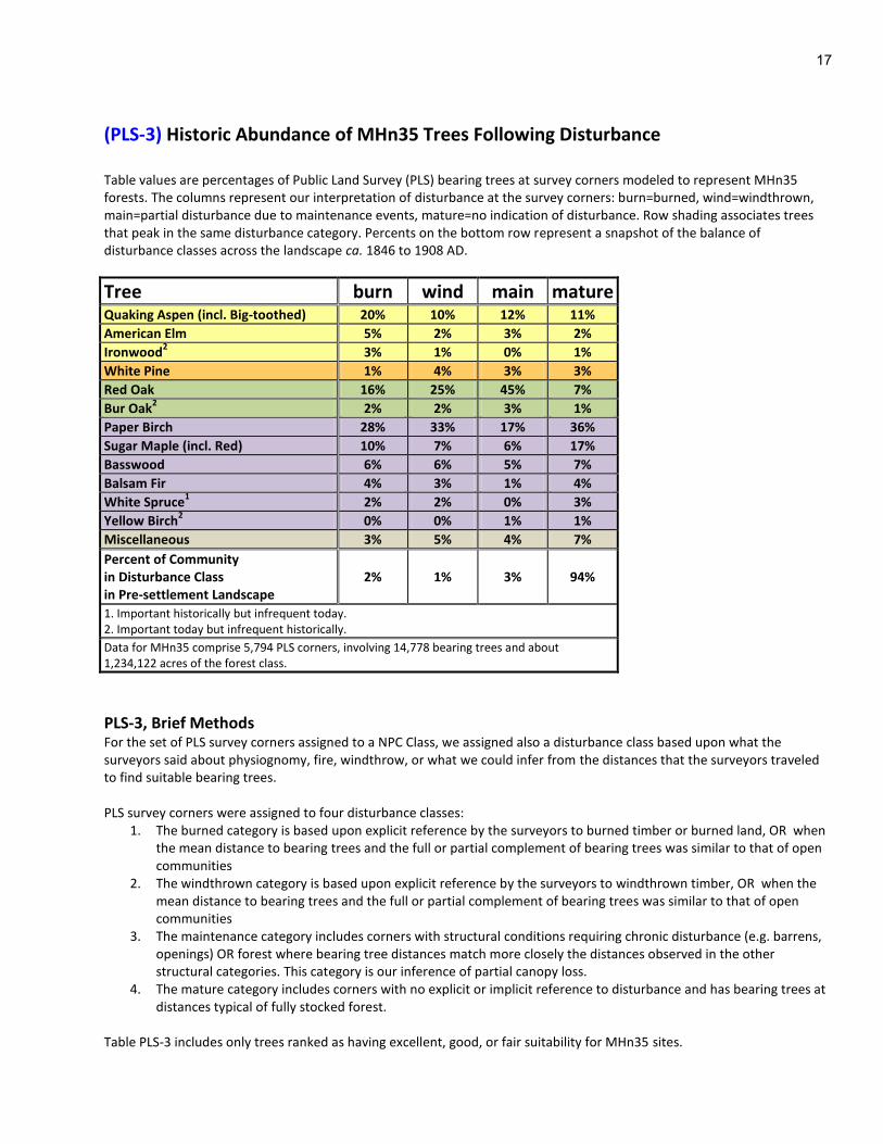
(PLS-3) Historic Abundance of MHn35 Trees Following Disturbance Table values are percentages of Public Land Survey (PLS) bearing trees at survey corners modeled to represent MHn35 forests. The columns represent our interpretation of disturbance at the survey corners: burn=burned, wind=windthrown, main=partial disturbance due to maintenance events, mature=no indication of disturbance. Row shading associates trees that peak in the same disturbance category. Percents on the bottom row represent a snapshot of the balance of disturbance classes across the landscape ca. 1846 to 1908 AD.

Tree burn wind main mature Quaking Aspen (incl. Big-toothed) 20% 10% 12% 11%

American Elm 5% 2% 3% 2%

Ironwood2 3% 1% 0% 1%

White Pine 1% 4% 3% 3%

Red Oak 16% 25% 45% 7%

Bur Oak2 2% 2% 3% 1%

Paper Birch 28% 33% 17% 36%

Sugar Maple (incl. Red) 10% 7% 6% 17%

Basswood 6% 6% 5% 7%

Balsam Fir 4% 3% 1% 4%

White Spruce1 2% 2% 0% 3%

Yellow Birch2 0% 0% 1% 1%

Miscellaneous 3% 5% 4% 7%

Percent of Community in Disturbance Class in Pre-settlement Landscape

2% 1% 3% 94%

1. Important historically but infrequent today. 2. Important today but infrequent historically.


PLS-3, Brief Methods For the set of PLS survey corners assigned to a NPC Class, we assigned also a disturbance class based upon what the surveyors said about physiognomy, fire, windthrow, or what we could infer from the distances that the surveyors traveled to find suitable bearing trees. PLS survey corners were assigned to four disturbance classes:

1. The burned category is based upon explicit reference by the surveyors to burned timber or burned land, OR when the mean distance to bearing trees and the full or partial complement of bearing trees was similar to that of open communities

2. The windthrown category is based upon explicit reference by the surveyors to windthrown timber, OR when the mean distance to bearing trees and the full or partial complement of bearing trees was similar to that of open communities

3. The maintenance category includes corners with structural conditions requiring chronic disturbance (e.g. barrens, openings) OR forest where bearing tree distances match more closely the distances observed in the other structural categories. This category is our inference of partial canopy loss.

4. The mature category includes corners with no explicit or implicit reference to disturbance and has bearing trees at distances typical of fully stocked forest.

Table PLS-3 includes only trees ranked as having excellent, good, or fair suitability for MHn35 sites.

18


1. Interpret the disturbance regime of the community and its normal successional model a. In general, communities with over 90% of their historic landscape in the mature category exhibit

succession and have trees able to regenerate in small canopy gaps that were not notable in the survey notes. Succession happens because the rotation (>150 years) exceeds the longevity of initial cohort trees.

b. In general, communities with under 90% of their historic landscape in the mature category have trees able to regenerate in equally well in the open or in large canopy gaps. Succession happens largely because of differences in longevity of initial-cohort trees with white pine, red pine, and oak outliving all aspens, paper birch, and jack pine.

c. In general, communities where the sum of mature and maintenance percentage exceeds 95% have strong dominants that constantly occupy those sites: sugar maple, ash, tamarack, black spruce. Succession usually involves changes in minor species about a core population of the site dominant.

2. Estimate which species are likely to respond positively, given a certain disturbance a. In general species with a high percentage in a disturbance column are likely to respond positively to a

prescriptive disturbance similar to the natural one. i. High fire percentage: open or large gaps with site preparation

ii. High windthrow percentage: open or large gaps without site preparation iii. High maintenance percentage and fire>wind: large gaps with site preparation iv. High maintenance percentage and wind>fire: large gaps with no site preparation v. High mature percentage: small gaps over advance regeneration

b. It may be equally important to consider species with low percentages in a disturbance column if the goal is to diminish their populations in the future forest.

19

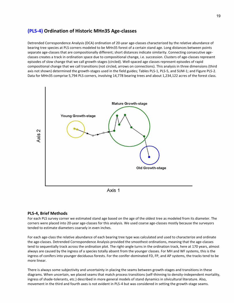
(PLS-4) Ordination of Historic MHn35 Age-classes Detrended Correspondence Analysis (DCA) ordination of 20-year age-classes characterized by the relative abundance of bearing tree species at PLS corners modeled to be MHn35 forest of a certain stand age. Long distances between points separate age-classes that are compositionally different; short distances indicate similarity. Connecting consecutive age-classes creates a track in ordination space due to compositional change, i.e. succession. Clusters of age-classes represent episodes of slow change that we call growth-stages (circled). Well-spaced age classes represent episodes of rapid compositional change that we call transitions (not circled, arrows on connections). This analysis in three dimensions (third axis not shown) determined the growth-stages used in the field guides; Tables PLS-1, PLS-5, and SUM-1; and Figure PLS-2. Data for MHn35 comprise 5,794 PLS corners, involving 14,778 bearing trees and about 1,234,122 acres of the forest class.

PLS-4, Brief Methods For each PLS survey corner we estimated stand age based on the age of the oldest tree as modeled from its diameter. The corners were placed into 20-year age-classes for this analysis. We used coarse age-classes mostly because the surveyors tended to estimate diameters coarsely in even inches. For each age-class the relative abundance of each bearing tree type was calculated and used to characterize and ordinate the age-classes. Detrended Correspondence Analysis provided the smoothest ordinations, meaning that the age-classes tend to sequentially track across the ordination plot. The right-angle turns in the ordination track, here at 170 years, almost always are caused by the ingress of a species totally absent from the younger classes. For MH and WF systems, this is the ingress of conifers into younger deciduous forests. For the conifer-dominated FD, FP, and AP systems, the tracks tend to be more linear. There is always some subjectivity and uncertainty in placing the seams between growth-stages and transitions in these diagrams. When uncertain, we placed seams that match process transitions (self-thinning to density-independent mortality, ingress of shade-tolerants, etc.) described in more general models of stand dynamics in silvicultural literature. Also, movement in the third and fourth axes is not evident in PLS-4 but was considered in setting the growth-stage seams.

20

PLS-4, Silvicultural Applications 1. Define periods of stable forest composition known as growth-stages

a. Growth-stages were constructed primarily for the purpose of simplifying and communicating the natural stand dynamics of a NPC Class.

b. In general, significant mortality is not anticipated during growth-stages and silvicultural treatments during those episodes should be aimed mostly at increasing quality more so than volume or compositional change.

2. Define periods of transition characterized by mortality and replacement a. In general, transitions are the episodes where commercial harvesting of species in decline is important if

timber productivity is the primary management goal. b. In general, transitions are the best window of opportunity for silvicultural manipulation through

commercial harvesting. c. In general, a managed transition (flux harvesting) should start about 10 years before the natural

transition. 3. Communicate silvicultural ideas by growth-stage

a. The growth-stages and transitions evident in PLS-4 are the main way to simplify, organize, and discuss natural stand dynamics and ecological processes that might be emulated by silvicultural treatments.

b. Most of the PLS-4 figures illustrate the reality of continuous compositional change that has been oversimplified for comparable discussions among the NPC Classes.

21

(PLS-5) Historic Windows of Recruitment for MHn35 Trees Windows of recruitment are stretches of contiguous age classes where for each species we find it to be the smaller-diameter tree at a PLS survey corner with at least one tree twice its diameter at the same corner. For the small-diameter tree, we interpret this situation as their establishment and growth in response to a disturbance or condition that post-dates the disturbance or condition that established the larger tree(s). The table presents the window of peak recruitment followed by comparative success in standard windows that match growth stages and assumed recruiting environment: PD=post-disturbance recruitment in an open environment, SSG=small sub-canopy gap recruitment during self thinning, LG=large gap recruitment during breakup of the initial-cohort canopy, SG=small gap recruitment in mature or old-growth forest. Row shading associates species that have peak recruitment in the same standard window.

Tree

Peak years

Young Transition Mature

0-15 yrs 15-55 yrs 55-95 yrs >95 yrs

PD SSG LG SG

Paper Birch 0-20 Excellent Good Fair to 80 --

Basswood 0-20 Good Fair Poor to 70 --

White Pine 0-20 Fair Poor -- --

Quaking Aspen (incl. Big-toothed) 0-30 Excellent Good Poor to 60 --

Red Oak 20-40 Poor Fair Poor to 70 --

American Elm 20-40 Poor Fair Poor to 80 --

Sugar Maple (incl. Red) 20-50 Fair Good Poor to 90 --

Ironwood2 30 Fair Good Fair Fair

Balsam Fir 40 -- Good -- --

Bur Oak2 50 -- Fair Poor to 70 --

Yellow Birch2 60-70 -- -- Poor --

White Spruce1 >100 -- Poor from 30 Fair Good

1. Important historically but infrequent today. 2. Important today but infrequent historically.



PLS survey corners modeled as belonging to a NPC Class were placed into 10-year age classes based upon the age of the oldest bearing tree as estimated from its diameter. For each age class, bearing trees were placed in two categories: larger diameter trees that could be in the same cohort as the oldest tree and small diameter trees that were most likely established and recruited to bearing tree size well after the event that established the oldest tree. The rule for placing a bearing tree into the small-diameter, recruit class was that its diameter was equal to or less than half the diameter of the largest bearing tree at the same corner. For each species, we plotted the abundance of its small-diameter recruits through time. The remarkable result was that the presence of recruiting trees was consistently in sets of contiguous age classes, and no tree had recruits in all age classes – this was true even of species present as trees throughout the course of succession. We decided to call the range of contiguous age-classes with recruits “windows of recruitment.” The peak years of recruitment were inferred from the shape (not magnitude) of the recruitment curves. The peak years are generally those with about 2-4 times the number of recruits in comparison to age-classes that seemed to represent a base-level of recruitment. We aligned growth-stages and windows of recruitment so that we could communicate recruitment concepts using the growth-stages and transitions as a familiar framework. Each species was assigned a recruitment rating based upon the magnitude of its recruitment peak: excellent (>10% of all bearing trees were recruiting individuals of that species), good (5-10%), fair (1-5%), poor (<1%).

22

General description of the four standard recruitment windows:

1. Post-Disturbance (PD) window: aligned with the initial years of the young growth-stage. This window represents a time where intolerant seedlings and sprouts of trees of any tolerance are recruited by out-competing herbs, shrubs, and inferior trees to occupy all available growing space.

2. Small Subcanopy Gap (SSG) window: aligned with the later years of the young-growth stage. This window represents a time where canopy trees are self-thinning and overtopped trees are being eliminated from the subcanopy individually. Trees with at least some shade tolerance are established and recruited mostly in reaction to increased levels of diffused light.

3. Large Gap (LG) window: aligned with the first transition. This window represents a time of fairly synchronous mortality of initial-cohort, canopy trees. Advance regeneration of mid- and shade-tolerant species are recruited in few-to-many tree gaps.

4. Small Gap (SG) window: aligned with mature and old growth-stages and presumably, maximum development of a canopy and subordinate strata. This window represents a time where only shade-tolerant trees can recruit into single-few tree gaps. Usually, the pool of possible recruits consists of well-developed and tall, saplings or poles.


1. Identify silvicultural systems that would favor recruitment of selected crop species a. In general, species with high ratings in the PD window are favored by clear-cutting, patch

cutting, and seedtree systems. b. In general, species with high ratings in the LG window are favored by shelterwood systems. c. In general, species with high ratings in the SG window are favored by selection systems.

2. Identify silvicultural treatments that favor recruitment of selected crop species when regeneration is present.

a. In general, species with high ratings in the PD window can be favored by selection of superior trees followed by weeding or cleaning.

b. In general, species with high ratings in the SSG window are favored by allowing young stands to remain overstocked until there is adequate advance regeneration, which then may be released by thinning or cleaning treatments.

c. In general, species with high ratings in the LG and SG window can be favored by matching their gap-size requirements to practices such as cleaning, or thinning.

3. Identify species that might do well when underplanted a. In general, all important species that are not usually part of the initial-cohort could, at some

time, be under-planted when a stand has been readied to meet their LG or SG requirements 4. Schedule examinations to assess recruitment and determine silvicultural action

a. In general, stands should be examined during the initial years of the PD window to assess stocking, survival of planted stock, and to contemplate thinning, weeding, or cleaning.

b. In general, stands should be examined during the initial years of the SSG window to assess ingress of SSG species and to contemplate underplanting or release.

c. In general, stands should be examined near the end of the SSG window to assess condition of the initial cohort, stocking of advance regeneration of SSG and LG species, and to contemplate harvest of initial cohort trees in a way that would favor them (most trees removed), LG species (about half of the trees removed), or SSG species (about a third of the trees removed or no harvest).

d. In general, stands are examined throughout the SG window to assess advance regeneration, condition and quality of crop trees, and to contemplate harvests aimed at regeneration or treatments aimed at improving quality.

23

(PLS-6) Natural disturbance rotations for Northern Mesic Hardwood Forests Natural rotations are the length of time it takes to disturb an area equivalent to the range of the Native Plant Community. Rotations are presented for three different kinds of disturbance: stand-replacing fire (fire), stand-replacing windthrow (wind), and less severe disturbances that maintain forest communities (main).

Northern Mesic Hardwood Forests Fire Main Wind

Northern Mesic Hardwood Forest – MHn35 966 yrs 131 yrs 1,278 yrs

Northern Wet-mesic Boreal Hardwood Forest – MHn44 428 yrs 160 yrs 957 yrs

Northern Mesic Hardwood (Cedar ) Forest – MHn45 3,095 yrs 3,095 yrs 3,095 yrs

Northern Wet-mesic Hardwood Forest – MHn46 604 yrs 194 yrs 805 yrs

Northern Rich Mesic Hardwood Forest – MHn47 1,820 yrs 329 yrs 1,971 yrs Data for MHn35 comprise 5,794 PLS corners, involving 14,778 bearing trees and about 1,234,122 acres of the forest class.


PLS survey corners modeled as belonging to a NPC Class were interpreted as to whether they were in a forest that had recently been disturbed. The PLS field notes contain several bits of information that help us detect disturbance:

1. Often the surveyor explicitly said in the line summary notes that the corner fell within burned or windthrown forest.

2. More often the surveyor described the physiognomy of the vegetation in a way that implies disturbance. For example, barrens, openings, scattered timber, etc. are known to be maintained by fire.

3. Threshold distances to the bearing trees indicate sparse stocking levels that are not typical of undisturbed forest. 4. When surveyors could not find enough bearing trees to completely reference a corner they often said so, meaning

it is fair to assume that a disturbance caused the lack of suitable trees in a quadrant. The goal of the analysis was to construct rules based upon the bits of information to assign each survey corner into one of four disturbance categories:

1. regenerated by catastrophic fire 2. regenerated by catastrophic wind 3. partially disturbed in some way by surface fire, selective windthrow, disease, pests, etc. 4. apparently undisturbed forest

This yields a set of survey corners modeled to be a particular NPC class and assigned to a disturbance class. Each corner represents about 213 acres of land that taken together comprise the entire statewide range of the community. This range is the base area for calculating rotation. Rotation is the number of years that it takes to disturb an area equal to the statewide range. Because we have three categories of disturbance, we can calculate three different rotations attributable to each kind of event. Rotations can also be calculated for combinations of those events (e.g. all fires or any disturbance). At this point, we know the proportion of the range represented in each disturbance category. If we felt that the surveyors only described disturbances in the same year that they happened then rotation is the inverse of the proportion. For example, if one-hundredth (0.01) of the range was burned it would take 100 years to burn the whole range. If however, we felt that surveyors would mention a fire up to 2 subsequent years, then the proportion 0.01 represents two years worth of fires, the annual proportion is 0.005, and the rotation 200 years. The number of recognition years that we assume is called the “window of recognition” and it greatly affects the calculations. Researchers have found a 15-year window to yield rotations that reasonably match rotations calculated from more reliable methods such as fire-scars and charcoal in varved lake sediments. We used the standard 15-year window to calculate catastrophic disturbance rotations, and we found that a 5-year window yielded reasonable rotations for maintenance disturbances.

24


1. Understand the geography of disturbance in Minnesota a. In general, the trend of disturbance rotation in Minnesota is for frequent, low-intensity events in

the southwest grading to infrequent, high-intensity disturbance in the northeast. b. In general, landforms and parent material affect rotation at a finer scale with flat, sandy

landforms having shorter rotations and hilly, loamy terrain having longer rotations. c. Because each cover type can be expressed in several different NPC classes, a comparison of

natural rotations among the classes can help us understand how site and geography affect commercial rotation – why it is shorter in some places and longer in others even though the same species is dominant.

2. Help create fire-regime maps for planning and fire response a. Landform maps where each landform has been assigned a matrix NPC class and its fire rotation

can be used to anticipate and plan fire response. 3. Examine the difference between natural and commercial rotation on landscape age-class distributions

a. Usually, this is done to set rotation parameters in equilibrium models to guess at the departure of historic conditions and modern ones driven by commercial rotation.

b. Most often, the modeling results are interpreted as to their effect on wildlife populations. 4. Match silvicultural systems and treatments to NPC classes to emulate the timing and severity of

disturbance a. In general, communities for which catastrophic rotation is about equal to that of maintenance

rotation can be “naturally” managed with even-aged systems like clearcutting with reserves or with two-step systems like the shelterwood system.

b. In general, communities for which catastrophic rotation is about twice or three times that of maintenance rotation can be “naturally” managed with three basic strategies:

i. To maintain early successional species clear-cutting with reserves or shelterwood systems would emulate a common natural disturbance.

ii. To maintain the late-successional species, systems that maintain a multi-aged stand could be used, with and entry schedule approximating the maintenance rotation.

iii. To allow a full successional cycle or convert a young stand to an older composition, silvicultural treatments can be used to emulate the natural removal of old early-successional species to release younger late-successional species. The entry schedule for this “flux” harvesting is set by the condition of trees and advance regeneration – not rotation.

c. In general, communities for which catastrophic rotation is four or more times that of maintenance rotation can be “naturally” managed with selective systems.

i. Because selective systems have been used so infrequently compared to clear-cutting, “flux” treatments are often needed to bring the community back to dominance of late-successional species.

ii. The entry schedule is far more frequent than maintenance rotation, and both harvesting and treatments are aimed at improving quality or managing advance regeneration. For an unknown reason, the maintenance rotation often approximates the biological longevity of the dominant, late-successional trees.

using public land survey (pls) records for...

Documents