various approaches for solving problems in heat conduction

Various Approaches for Solving Problems in HeatConduction with Phase Change

Mohamad MUHIEDDINE†?

†IRISA, Campus de Beaulieu? Archeosciences, UMR 6566

35042 Rennes, France

[email protected]

Edouard CANOT†

†IRISA, Campus de Beaulieu35042 Rennes, France

[email protected]

Ramiro MARCH?

? Archeosciences, UMR 656635042 Rennes, France

[email protected]

Abstract

This paper treats a one dimensional phase-change problem, ’ice melting’,by a vertex-centered finite volume method. Numerical solutions areobtained by using two approaches where the first one is based on the heatconduction equation with the basic grid (improved by introducing a newadaptive mesh technique), latent heat source approach (LHA), while thesecond uses the equivalent thermodynamic parameters defined by consid-ering the apparent heat capacity method (AHC). A comparison betweenthe two approaches is presented, furthermore the accuracy and flexibilityof the numerical methods are verified by comparing the results withexisting analytical solutions. Results indicate that phase-change problemscan be handled easily with excellent accuracies by using the AHC method.

Key words : Phase-change, computational fluid dynamics, latentheat, finite volumes, rolling mesh, self-adaptive mesh, apparent capacitymethod, moving boundary problem.

International Journal on Finite Volumes, vol. 6, n. 1

Phase Change Problem

Nomenclature

Cp : Specific heat,E : Energy,H : Total enthalpy,T : Temperature,k : Thermal conductivity,L : Latent heat of fusion,U : Step function,V : Control volume,Q : Accumulation latent heat,

Qtotal : Total latent heat,∆x : Control volume size,∆φ : Heat flux difference,∆t : Time step,∆T : Temperature semi-interval,α : Weighting factor,θ : Solid fraction,ρ : Density,φ : Volumetric fraction,ξ : Interface position,δ : Dirac delta function.

Subscripts0 : Initial phase,f : Phase changing point,i : node index,l : Liquid phase,s : Solid phase.

1 Introduction

Melting processes are classified as moving boundary problems which have been ofspecial interest due to the inherent difficulties associated with the non-linearity ofthe interface conditions and the unknown locations of the moving boundaries. Thispaper is concerned with a numerical method for solving a one dimensional phase-change problem leading to further studies on energy-saving and quality improve-ments. Solving such problem of phase change, where analytical solution exists,enables us to choose the best approach to solve our problem of interest “the forcedevaporation in saturated porous media” which has a direct application in the studyof prehistoric fire.

Over the years, a number of related computational works have employed varioustechniques in the analysis of phase change problems. Several important theoreticalresults on the existence, the uniqueness and the properties of classical solutions areavailable in the literature [MUE 65], [CAN 67], [LUI 68], [BEJ 03]. Besides, mostanalytical solutions deal with for 1-D geometries with very particular boundaryconditions hence, cannot be generalize to multidimensional problems. Thus, many

International Journal on Finite Volumes 2


numerical schemes [VOL 87], [KIM 90], [WAN 00], [SAV 03], [JAV 06], have beenproposed to study transient heat conduction problems with phase change in one,two and three dimensions, but two formulations are predominant in the numericalanalysis. The first one is referred to as the ’front-tracking method’ in which the posi-tion of the moving front is determined at each time step [ASK 87], and must alwayscorrespond to a node or edges mesh. The use of this numerical method can usuallyeliminate the oscillations obtained by using the fixed grid method, and allows formore precise solutions. However, it is poorly suited to multi-dimensional problemsdue to the algorithm’s difficult implementation and the large computational cost.

The second formulation, based on the use of the heat enthalpy concept [BON 73],[PRA 04], recasts the problem in such a way that the conditions on the moving phasefront are absorbed into new equations, and the problem is solved without explicitreference to the position of the internal boundary (interface position). Its positionis determined a posteriori, when the solution is complete. The major problem withthe latter method is that it is not very accurate. In addition, this formulationoften requires the use of algorithms to correct the solution in order not to miss theabsorption or the release of latent heat.

Other publications related to heat conduction problems with phase change, usingeither finite difference or finite element method or both, can be found in references[PAW 85], [GRA 89], [SAV 03]. All of them are of interest, but the most interestingnumerical method in our case is based on the finite volume formulation which hasthe important feature that the resulting solution ensures that the conservation ofquantities involved such as mass, momentum and energy is exactly satisfied notonly over any group of control volumes but over the whole domain of computation,which is not the reality when dealing with finite difference methods. Finite elementapproach [GUI 74] takes advantage in the ability to divide the domain of interest inelementary subdomains, namely elements. It may therefore handle problems withsteep gradients and may deal with irregular geometric configurations. Comparingfinite element method with finite volume one, this last still more conservative andso more adequate to solve our problem.

This work chooses to use two approaches, the latent heat accumulation approach(LHA) [PRA 04] and the apparent heat capacity method (AHC) [BON 73]. Thenumerical methods based on enthalpy formulation of the problem have been studiedin [BON 73], [CIV 87], [LAM 04], [PRA 04], [MUH 08]. However, the algorithmproposed for the LHA method is rather similar to that of Prapainop [PRA 04],where the enthalpy formulation has been used to construct an approximation scheme.The finite volume method is implemented over a special rolling mesh in the LHAcomposed of a basic regular grid which is recursively refined near the interface. Inthe AHC a fixed grid scheme has been used.

2 Mathematical model for simulating problem with phasechange

Only conduction is considered as a heat transfer mode. The physical propertieswhich characterize the solid and liquid phase, such as specific heat and conductivity,



are constant for a given phase, it is likely not to be the case in reality but our modelis able to take into account non-constant parameters. This proposed approximationsupposes that all radiative effects within ice melting are neglected. In the following,we shortly describe equations for a melting problem, with the further approximationthat density is the same for the two phases.

2.1 Equations and boundary conditions

Our melting problem is characterized by solving the partial differential equationobtained by combining Fourier’s law of heat conduction and the law of conservationof energy which states that the rate of energy accumulation within a control volumeof size ∆x equals the net heat transfer by conduction

∂

∂t[ρCpT∆x] = ∆φ (1)

where ∆φ is the heat flux difference at the boundaries of the control volume. Theproblem deals with a semi-infinite region of ice initially at T0 = −10◦C. At timet > 0, the boundary at x = 0 is suddenly kept at Tw = 20◦C. The governingequations for the temperature T (x, t) are formulated as follows :ρCl

∂T

∂t=

∂

∂x

[kl

∂T

∂x

]0 < x < ξ (t) , t > 0

Tl(0, t) = Tw t > 0(2)

ρCs∂T

∂t=

∂

∂x

[ks

∂T

∂x

]ξ(t) < x < +∞, t > 0

Ts(∞, t) = T0 t > 0(3)

and for t = 0T (x, 0) = T0 ∀x ∈ [0,∞[

where ρ = ρs = ρl is the density, C is the specific heat, ξ(t) is the interface position,and the subscripts s and l indicate the solid and liquid phases, respectively.

At the interface, the heat flux condition is written as [BON 73] :

kl∂Tl

∂x− ks

∂Ts

∂x= −ρL

dξ

dtat x = ξ(t) (4)

where L is the latent heat coefficient and dξ/dt is the velocity of this interface.During the melting process, the liquid/solid front, which absorbs massive latent heat,continuously progresses through the medium. Moreover, the temperature verifies :

Tl = Ts = Tf at x = ξ(t)

where Tf is the melting temperature.At the initial time, the interface is assumed to be at position zero (i.e., ξ(0) = 0).



3 Analytical solution

Exact solutions of 1D phase change of a semi-infinite slab were analyzed by Carslawand Jaeger [CAR 59] and KU and Chan [KU 90] with the moving front approach.The exact temperature distributions in solid, Ts, and in liquid, Tl, are respectively :

Tl = Tw + (Tf − Tw)erf(x∗)erf(x∗sl)

when 0 < x∗ < x∗sl

Ts = T0 + (Tf − T0)erfc(

√µl/µsx∗)

erfc(√

µl/µsx∗sl)when x∗sl < x∗ < ∞

(5)

where x∗ = x/2√

µlt is the dimensionless position and µ = k/ρC is the thermaldiffusivity. The two values are calculated from corresponding mechanical propertiesfor both solid µs and liquid µl values. The values of dimensionless position of solid-liquid interface x∗sl are obtained via the nonlinear algebraic equation :

Tf − T0

Tf − Tw

ks

kl

√µl

µs

exp(−(µl/µs)(x∗sl)2)

erfc(√

µl/µsx∗sl)+

exp(−(x∗sl)2)

erf(x∗sl)−

√πx∗slL

Cl(Tf − Tw)= 0 (6)

4 Numerical method

The set of equations presented above are cast in the usual finite volume form for afinite domain (actually of length 2 m), under a vertex centered formulation: eachcell (or control volume) encloses exactly one data node at xi and its boundariesare always computed as the center of two consecutive nodes, so that we obtain agood accuracy in the gradient estimation. We denote by Ti the whole approximatesolution, the location of any variables being indicated by subscripts.

The time domain is divided into an arbitrary number of constant time steps ofsize ∆t. Variables at time t are indicated by the superscript 0. In contrast, thevariables at time level t + ∆t are not superscripted.

For instance, the temperature at face i + 12 is Ti+ 1

2= Tifi+ 1

2+ Ti+1

(1− fi+ 1

2

)where fi+ 1

2= (2δxi+ 1

2− ∆xi)/2δxi+ 1

2, ∆xi = xi+ 1

2− xi− 1

2, δxi+ 1

2= xi+1 − xi,

and δxi− 12

= xi − xi−1 as schown in figure 1). The other variable that has to beapproximated at cell faces is the interface conductivity; the harmonic mean is usedfor composite materials for its superior handling of abrupt property changes byrecognizing that the primary interest is to obtain a good representation of heat fluxacross interfaces rather than that of the conductivity [PAT 80] :

1k

=1− fi+ 1

2

ki+

fi+ 12

ki+1(7)

In this study, the temporal distributions of temperature is approximated by two-timelevel schemes [VER 95], such that :∫ t+∆t

tTdt =

[αT − (1− α)T 0

]∆T (8)



where α is a weighting factor with the value between 0 and 1.Three main schemes are considered: explicit, Crank-Nicholson and fully implicit.

The first-order accurate explicit method uses temperature gradients of the previoustime step t to calculate the unknown T at t + ∆t such that α = 0. Hence, the timestep size ∆t is limited to ∆t < ρc(∆x)2/2k for 1D. The second-order accurate Crank-Nicholson scheme uses the average of previous and present temperature gradients tocompute the present temperature, by taking α = 0.5 in the above, and hence, hasless severe step size limitation than the explicit scheme. The fully implicit scheme ,however is unconditionally stable with first-order accuracy at α = 1.

Taking Figure 1 as reference, the heat equation may be discretized as follows :

ρc∆xi

(Ti − T 0

i

)=

[ki+ 1

2

α (Ti+1 − Ti) + (1− α)(T 0

i+1 − T 0i

)δxi+ 1

2

− ki− 12

α (Ti − Ti−1) + (1− α)(T 0

i − T 0i−1

)δxi− 1

2

]∆t.

(9)

Figure 1: A typical 1D control volume

The convergence and stability of this kind of method could be proven accordingto the work of [MAG 93].

5 Problem reformulation and Latent heat accumulationmethod

In the basic enthalpy scheme, enthalpy is used as the primary variable and thetemperature is calculated from a defined enthalpy-temperature relation :

H ={

ρCsT, T < Tf

ρCsTf + ρCl (T − Tf ) + ρL, T ≥ Tf(10)

where H is the enthalpy.Anticipating the discrete description given in the next section, we suppose now

that the physical domain (one dimensional in our case) is divided into a finite numberof cells (from now on, the subscript i refers to a particular volume).

The latent heat accumulation method has been proposed by [PRA 04] and isresumed hereafter. Prior to the first time interval, the accumulated latent heat Qi

of a control volume Vi is initialized to zero. At the beginning of each time step,the phase status of each control volume is checked. If the nodal phase is solid



and the nodal temperature Ti rises higher than the melting temperature Tf , thencontrol volume becomes saturated and its node is tagged (the cell is called “mushy”).Since an explicit scheme is used, the current temperature may be calculated directlyfrom the previous values. The nodal temperature is then reassigned to the meltingtemperature and the latent heat increment (the energy used for phase change in thecurrent time step) is calculated from the fictitious sensible heat such that ∆Qi =ρC (Ti − Tf ) Vi, where Vi is the volume of the cell and C is calculated as follows:C = (1 − θ)Cl + θCs, where the solid fraction θ is the percentage of ice present inVi.The ∆Qi quantity is added to the accumulated Qi for subsequent time steps untilthe accumulated latent heat equals the total latent heat Qtot

i available in the controlvolume, which is

Qtoti =

∫Vi

ρLdv (11)

At this stage, the control volume becomes liquid, the tag on the cell is removed andthe latent heat increment is no longer calculated.

5.1 Basic model with uniform mesh

As a first step, the discretized formula obtained has been applied under the explicitform where the time step must be chosen according to the Cauchy stability criterion:

∆t < ∆tc =12

ρsCs∆x2

ks

Practically, ∆t is always chosen to be equal to 0.99∆tc.Thermophysical properties used in the calculation are those of the system wa-

ter/ice. Spatial temperature profiles (Figure 2a; only a quarter of the whole domainis shown) match the analytical solution [PRA 04] very well, but time evolutions (Fig-ure 2b) present some fluctuations, despite the large number of nodes used. Thesefluctuations are unavoidable: they are due to the finite width of the cell (In fact, theheat flux is blocked during the melting process inside the mushy cell). To overcomethis unwanted behavior, the only way is to refine the grid near the interface, leadingto the adaptive mesh technique presented below.

5.2 Improved model with recursive mesh refinement

It becomes obvious that in order to prevent any non-physical solution, it is advan-tageous to vary the mesh size according to the position of the interface. A globalrefinement would be the simplest technique in order to enhance the accuracy of theapproximated solution; however, this technique will not be used here due to the highmemory required. In general, two types of adaptive techniques are mostly used; thefirst one is the local refinement method whereby uniform fine grids are added in theregions where the approximated solution lacks adequate accuracy [ASK 87], and thesecond is the moving mesh technique where nodes are relocated at necessary timesteps [MER 00].



(a) Temperature profile at tmax = 50 h. (b) Temperature history at x = 5 cm.

Figure 2: Uniform mesh, Nbasic = 200, dt = 4.46E + 01 s. Analytical (red) and numerical(blue) solutions.

We have chosen a different technique, a classical ’insert/delete nodes’ techniquefor the primal mesh (like Homard [HOM 95], used in FEM but adapted for thefinite volume schemes) which has been used with recursive subdivisions, to produceexcellent results for the one-dimensional melting problem. The previously describedfixed basic uniform mesh is our starting point; then we refine the primal mesh by anumber of subdivisions near the phase-change front — at each level of subdivion weadd a node at the middle of the two successive nodes (see Figure 3). The meltingfront is initially located in the first cell and can move anywhere along the discretizeddomain. When the phase-change front transfers to a new cell, the node added in aprevious step is removed and a new node will be added to the new element.

This rolling mesh has the following characteristics:

• the mesh rolls because some nodes are added whereas others are deleted, butonly when the mushy cell changes; most of the time the whole mesh remainsunchanged;

• only the primal mesh is locally refined; then the dual mesh (i.e., the cellboundary) is updated;

• it is not a moving mesh: during the time evolution all nodes are fixed inposition. This fact guarantees a good accuracy due to the small number ofneeded interpolations (they are needed only when a new node is inserted).

This technique was implemented as a double linked list in Fortran 95. Each itemof this list contains information about geometry (cell size) and physical variables(temperature, latent heat accumulation and a tag for the phase state). A numberof fixed recursive subdivisions is used depending on the precision needs.



Figure 3: Recursive mesh refinement used to track the phase change front (dot points arenodes whereas dashed lines delimit cells; the mushy cell is colored in grey). Blue points arethe basic uniform mesh. Circled points are the new nodes which have been inserted (betweensteps 1 and 2) to satisfy some constraints on the mesh progressiveness. The crossed pointdisappears between steps 2 and 3.

5.3 Energy conservation during the ’insert/delet nodes’ technique

It is well known that the finite volume scheme conserves some extensive quantities.In our case, it is namely the energy used in equation 1, that can be written as follows

E =∫

ρCTdx (12)

As in our physical model ρ and C are constants (in each phase), the integral oftemperature must be conserved over the whole mesh during any ’insert/delete’ nodesevent.

Suppose we must insert a new node or delete an existing one: other tempera-ture values at other nodes should be then modified for E to be remain unchanged.However, in our refinement technique (described in the previous subsection), weadd/delete a node only for the ’mushy’ cell (corresponding to a slope discontinuityof the temperature) without any modification. This is because a node is alwaysinserted (or deleted) in a linear temperature behavior as we can see in Figures 4a or5a.

5.4 Results and comments

We have found that the adaptive technique do ameliorates the smoothness (hencethe correctness) of the solution. Figures 4 and 5 show numerical results for twodifferent values of the subdivision number. The more we refine the phase-changearea, the more we obtain a good accuracy and fewer fluctuations; actually thesefluctuations are not eliminated but their amplitude decreases drastically that theyseem to vanish (see Figure 7). A good agreement with the analytical solution isshown.

Figure 6a clearly indicates that the local mesh refinement allows the use of a lesstotal number of nodes leading to an economy of memory usage. It also shows errorsbetween the numerical and the analytical solutions, and gives a comparison betweenthe two models used. The relative error is calculated only from the time evolutioncurve (at x = 5 cm) via the following Root-Mean-Square formula:

ErrorRMS =

√√√√ 1N

N∑j=1

(T (tj)− T (tj)exact)2.



N being the total number of time steps.Globally, taking into account both precision and computational cost, the pro-

posed scheme is slightly better than the basic one, as shown in Figure 6b. Actually,the performance limitation of our method is due to the use of an explicit schemewhich requires us to use a small time step; this should be numerically expensive inthe case of large problems. Therefore, this method is poorly suited to multidimen-sional problem.


Figure 4: Rolling mesh, Nbasic = 40, dt = 1.74E + 01 s, number of subdivisions: 3.Analytical (red) and numerical (blue) solutions.


Figure 5: Rolling mesh, Nbasic = 40, dt = 2.72E − 01 s, number of subdivisions: 6.Analytical (red) and numerical (blue) solutions.

Due to the limitation of the explicit scheme, several implicit ones have been tried(Crank-Nicholson and a fully implicit scheme) to achieve the expected efficiency andcomputational cost. As previously described, the explicit scheme has a restriction ontime step size. Moreover, large time intervals cause the solution to diverge. Crank-Nicholson and fully implicit schemes may employ somewhat larger time steps butbecause of the structural model accuracy still depends on time step sizes. In addition,



(a) RMS Errors versus the total number ofcells.

(b) RMS Errors versus the computationaltime.

Figure 6: explicit scheme.

implicit schemes require more CPU time than the explicit scheme due to the iterativeprocedures of the solver. Figure 8 shows the limitation of the used approach withthe implicit schemes, thus a need of a different approach. However, by using thisapproach it is difficult to determine the interface position in multidimensional case.

10−4

10−3

10−2

10−1

10−1

100

∆ xmin

Err

or m

ax (

T(t

))

Figure 7: Oscillations amplitude on temper-ature history.

10−4

10−2

100

102

104

10−3

10−2

10−1

100

101

102

CPU time (s)

ε (%

)

explicit schemeimplicit schemeCrank−Nicholson scheme

Figure 8: RMS Errors on the temperaturehistory versus the CPU time.

6 Apparent heat capacity method

To avoid the tracking of the interface, the apparent heat capacity method will beused. In this method, the latent heat is calculated by integrating the heat capacityover the temperature [BON 73], and the computational domain is considered as oneregion. As the relationship between heat capacity and temperature in isothermal



problems involves sudden changes, the zero-width phase change interval must be ap-proximated by a narrow range of phase change temperatures. Thus, the size of timesteps must be small enough so that this temperature range is not overlooked in thecalculation. The equivalent thermodynamic parameters are defined considering theapparent capacity method of [BON 73]. According to this reference, if these prop-erties do not depend on temperature, the equivalent parameters may be obtainedtaking into consideration that the phase change takes place in a small temperatureinterval (see Figure 9 ).

Figure 9: Physical properties given byBonacina.

Figure 10: Smoothed physical propertiesused in this paper.

Then, if this interval is ∆T :

C =

Cs, T < Tf −∆T

Cl+Cs

2 + L2∆T , T f −∆T ≤ T ≤ Tf + ∆T

Cl, T > Tf + ∆T

(13)

Where L is the heat of phase change per unit volume [J/kg], Tf is the phase changetemperature, and ∆T is the temperature semi-interval across Tf . Similarly a globalnew thermal conductivity has to be introduced:

k =

ks, T < Tf −∆T

ks + kl−ks

2∆T [T − (Tf −∆T )] , T f −∆T ≤ T ≤ Tf + ∆Tkl, T > Tf + ∆T

(14)

Numerical solutions are obtained by using an approach based on a fixed gridand a vertex-centered finite volume discretization. The accuracy and flexibility ofthe present numerical method are verified by comparing the results with existinganalytical solutions. The principal advantages of this approach are that (i) temper-ature T is the primary dependent variable which derives directly from the solution,and (ii) the use of this method usually eliminates the fluctuations found by usingthe LHA approach (see figure 2b). However, the AHC formulation leads to approx-imated solutions and suffers from a singularity problem for the physical properties



C (specific heat capacity) and k (conductivity) (see Figure 9). While the explicitform of discretization used in the previous approach is computationally convenient,it has a possible limitation due to the presence of time fluctuations in the solution.Results show the limitation of the LHA method due to the limiting small time step.

The implicit calculation is often worthwhile because the implicit Euler methodhas no stability limit. However, there is a price to pay for the improved stabilityof the implicit method, which is solving a system of nonlinear ordinary differentialequations. We are going to solve PDEs by using the method of lines, where spaceand time discretizations are considered separately, leading to semi-discrete systemsof ODEs. Fortunately, there is a considerable amount of high quality ODE softwareavailable, much of it recently developed. These softwares are used for the integrationin t to achieve stability (or a more sophisticated explicit integrator in t is used thatautomatically adjusts ∆t to achieve a prescribed accuracy).

The numerical solution can be obtained as the limit of a uniformly convergentsequence of classical solutions to approximating problems, deduced by smoothingthe coefficients (13, 14), following few general rules [CIV 87]: The apparent heatcapacity formulation allows for a continuous treatment of a system involving phasetransfer. If the phase transition takes place instantaneously at a fixed temperature,then a mathematical function such as

φ = U(T − Tf ) (15)

is representative of the volumetric fraction of the initial phase (ice phase). U is astep function whose value is zero when T < Tf and one otherwise. Its derivative,i.e., the variation of the initial phase fraction with temperature, is

dφ

dT= δ(T − Tf ) (16)

in which δ(T−Tf ) is the Dirac delta function whose value is infinity at the transitiontemperature, Tf , but zero at all other temperatures.To alleviate this singularitythe Dirac delta function can be approximated by the normal distribution functionsketched in Figure 11

dφ

dT= (επ−1/2)exp[−ε2(T − Tf )2] (17)

in which ε is chosen to be ε = 1/√

2∆T and where ∆T is one-half of the assumedphase change interval. Consequently, the integral of equation 17 yields the errorfunctions approximations for the initial phase fraction as sketched in Figure 12. Withconventional finite volume method, the initial phase fraction derived from equation17 by integration should be used to avoid the numerical instabilities arising from thejump in the values of the volumetric fraction of initial phase from zero to one. In ourapproach we assume for simplicity that the phases are isotropic and homogeneous,and the densities of the phases are equal. Accordingly, the smoothed coefficients(see Figure 10) of equations 13 and 14 could be written as:

c = cs + (cl − cs)φ + Ldφ

dT(18)



Figure 11: Approximation of the initialphase fraction over a small temperature in-terval according to the linear functions.

Figure 12: Approximation of the initialphase fraction over a small temperature in-terval according to the error functions.

and

k = ks + (kl − ks)φ (19)

6.1 Global resolution using the Method of lines

The problem to be solved may be written in vectorial form with adequate initial andboundary conditions:

∂T

∂t= f(t, x, T ) (20)

The user is typically required to write a simple routine which evaluates the func-tion f when the arguments t, x, T, ∂T/∂x, ... are provided. Other equally simplesubprograms would be required to specify appropriate boundary and/or initial con-ditions.

With generalization in mind, a numerical strategy inspired by the treatment ofordinary differential equations (ODE) associated to space discretization using themethod of lines is applied [HUN 03]. It allows:- a global treatment of the system without discrimination between the variables.- a treatment of the physical model in its original form, as it was written, withoutpreliminary manipulations.- the use of sophisticated methods which have been developed for initial value dif-ferential equations.- the possibility, for further works, to use the developments involved in ODE systems(parameter estimation, sensitivity analysis...)

The main failures of the method are the large size of the resulting ODE systemobtained after discretization (this problem can be reduced by using an adequatenumerical conditioning of the system) and the rigidity of the fixed grid discretization



scheme which is not really a problem in our case and could be solved by using anadaptive mesh.

The numerical method of lines consists in discretizing the spatial variable intoN discretization points. Each state variable T is transformed into N variables cor-responding to its value at each discretization point. The spatial derivatives areapproximated by using a finite volume formula on 3 points where the best resultsfor accuracy and computation time efficiency were obtained. We are solving PDEs,where space and time discretizations are considered separately this lead to a semi-discrete system of ODEs, which can be written as:

T′= A(T )T (21)

The Jacobian matrix A(T ) is computed explicitly (its tridiagonal structure is dueto the 1-D laplacian discretization). The ODE solver has been modified in such away that the Jacobian matrix A(T ) could be coded by hand in sparse format. Thenumerical calculation is performed with ddebdf routine of the SLATEC Fortranlibrary [BRE 89]. This is designed to simulate systems of coupled non-linear andtime dependent partial differential equations. It is used for the time integration toachieve stability and a prescribed accuracy by adjusting automatically the time stepin the Backward Differentiation Formula (BDF). The BDF method is well adaptedto our problem which becomes more and more stiff as ∆T decreases (see Figure 16).

6.2 Results and comments

The accuracy and flexibility of the present numerical method are verified by com-paring the results with existing analytical solutions [BEJ 03]. Figures 13a and 14apresent the temperature profile for different values of ∆T , with spatial discretiza-tion N = 320. Figures 13b and 14b show the related histories of temperature atx = 5 cm. It is evident that the accuracy of the AHC method is sensitive to themagnitude of ∆T that is arbitrarily selected to approximate the Dirac delta functionor to distribute the latent heat.

We introduce a quality factor for each solution which combines accuracy andsmoothness according to the relation:

Quality factor = ErrorRMS(T ) + 0.025 ErrorRMS(T′) (22)

Since the apparent heat capacity method approaches the exact analytical solutionas the assumed temperature interval approaches zero, it is shown that the apparentheat capacity method can produce both smooth and accurate solutions.

It appears from these numerical solutions that the results obtained by approx-imating the phase change at a fixed temperature by a gradual change over a smalltemperature interval should be acceptable if

2∆T

|Ti − Tf |< 0.1 (23)

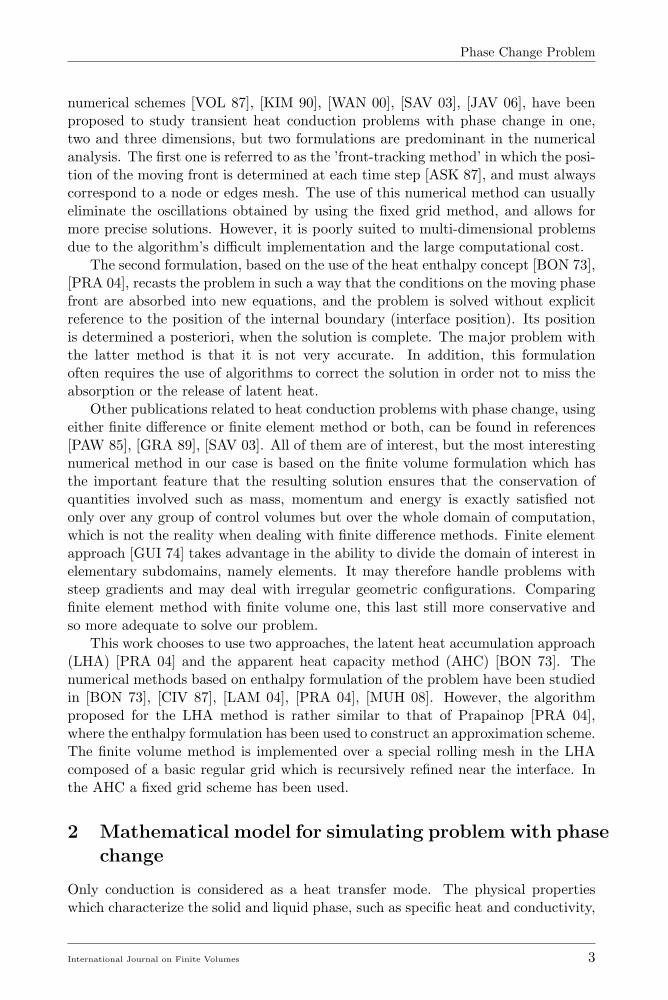
where Ti is the temperature of the control volume Vi.In Figure 15, we can see that there is a minimum for the quality factor corre-

sponding to an assumed value of ∆T . This minimum has been drawn as ∆x inFigure 17.




Figure 13: Nbasic = 300. ∆T = 0.1◦C. Analytical (red) and numerical (blue) solutions.


Figure 14: Nbasic = 300. ∆T = 0.5◦C. Analytical (red) and numerical (blue) solutions.

7 Comparison between the two methods

Practically in phase change situations, more than one phase change interface mayoccur or the interfaces may disappear entirely. Furthermore, the phase change usu-ally happens in a non-isothermal temperature range. In such cases, tracking thesolid-liquid interface may be difficult or even impossible. Calculation-wise, it isadvantageous that the problem is reformulated in such a way that the Stefan condi-tion is implicitly bounded up in a new form of the equations and that the equationsare applied over the whole fixed domain. This can be done by determining whatis known as the enthalpy function H(T ) and by using the AHC approach. TheLHA method has the great advantage which is the accuracy of the solution, butthis method suffers from fluctuations which are covered by a local refinement of thediscretization near the interface. The major problem of this method is that in nu-merical terms, we are using an explicit parabolic scheme, and this is very penalizingwhen used with adaptive refinement. For the moment, the problem is solved in 1-D.



0 0.2 0.4 0.6 0.8 10

0.5

1

1.5

2

2.5

∆ T

Qua

lity

Fac

tor

N = 81N = 161N = 321N = 601N=1241

Figure 15: Quality factor versus themagnitude of the assumed temperatureinterval for different number of nodes.

0 0.2 0.4 0.6 0.8 1

0

2

4

6

8

10

12

14

16

18

∆ T

CP

U T

ime

N = 81N = 161N = 321N = 601N=1241

Figure 16: CPU-Time versus the magni-tude of the assumed temperature intervalfor different number of nodes.

In 2 and 3 dimensions we can expect major difficulties in terms of implementation(in particular, the determination of the interface position) and cost (due to the useof an explicit scheme).

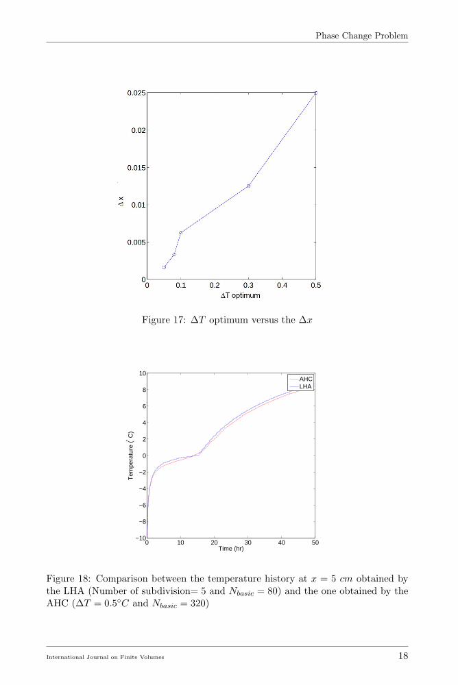
With the AHC approach, it is also possible to describe the non-isothermal phasechange. This proposed model is solved by using the method of lines with which thefluctuations found in the LHA approach can be avoided by choosing an appropriatevalue of ∆T . Otherwise, it is evident that the error and the order of precision ismore pronounced due to approximating the singularity (Dirac delta function) bya gradual change over a small temperature interval. Another observation is thatthe effect of distributing the latent heat over a temperature interval diminishes asthe ratio of temperature interval to the overall temperature variation of the systembecomes smaller. It is evident that the AHC method can produce accurate andsmooth solutions. Perhaps the biggest criticism to be lodged against this methodis that in its standard implementation it requires too much storage for each of theunknown quantities being computed. This would be quite excessive to the personinterested in solving a 3-D time dependent problem who is required to use onlyseveral locations per point in the problem. However, the presented approach forsolving non-linear heat conduction problems is very relevant and we can say thatwe are presenting one of the most efficient algorithms which takes into account thesimplicity of implementation and the desired accuracy. Examples have demonstratedthe accuracy reached. Figure 18, illustrates the temperature histories at x = 5 cmobtained by using the two presented approaches.



Figure 17: ∆T optimum versus the ∆x

0 10 20 30 40 50−10

−8

−6

−4

−2

0

2

4

6

8

10

Time (hr)

Tem

pera

ture

(° C)

AHCLHA

Figure 18: Comparison between the temperature history at x = 5 cm obtained bythe LHA (Number of subdivision= 5 and Nbasic = 80) and the one obtained by theAHC (∆T = 0.5◦C and Nbasic = 320)



8 Acknowledgement

This work has been done in the frame of ARPHYMAT1 collaboration, with a fi-nancial support from the “Ministere de l’Education Nationale et de la Recherche,France”.

9 Bibliography

[ASK 87] Askar H. G., (1987), “The front-tracking scheme for the one-dimensionalfreezing problem”, Int. J. of Num. Methods in Engng, Vol. 24, N. 5, pp 859-869.

[BEJ 03] Bejan A. and Kraus A. D.,(2003), Heat Transfer Handbook, Wiley.

[BON 73] Bonacina C., Comini G., Fasano A. and Primicerio M., (1973),“Numerical solution of phase-change problems”, Int. J. Heat Mass Transfer, Vol.16, N. 10, pp 1825-1832.

[BRE 89] Brenan K. E., Campbell S. L. and Petzold L. R., (1989), NumericalSolution of Initial-Value Problems in Differential-Algebraic Equations, Elsevier.http://www.netlib.org/slatec/index.html

[CAN 67] Cannon J. R. and Hill C. D., (1967), “Existence, uniqueness, stabilityand monotone dependence in a Stefan problem for the heat equation”, J. Math.Mech., Vol. 17, N. 1, pp 1-19.

[CAR 59] Carslaw H. S. and Jaeger J. C., (1959), Conduction of Heat in Solids,Oxford Clarendon Press.

[CIV 87] Civan F. and Sliepcevich C. M., (1987), “Limitation in the Apparentheat capacity formulation for heat transfer with phase change”, Proc. Okla. Acad.Sci., Vol. 67, 1987, pp 83-88.

[GRA 89] Grandi G. M. and Ferreri J. C., (1989), “On the solution of heatconduction problems involving heat sources via boundary-fitted grids”, Comm. inAppl. Num. Methods, Vol. 5, N. 1, pp 1-6.

[GUI 74] Comini G., Del Guidice S., Lewis R. W. and Zienkiewicz O. C.,(1974), “Finite Element Solution of Non-linear Heat Conduction Problems withSpecial Reference to Phase Change”, Int. J. Num. Methods in Engng, Vol. 8, N. 3,pp 613-624.

[HOM 95] Nicolas N., Arnoux-Guisse F. and Bonnin O., (1995), “Adaptivemeshing for 3D Finite Element Software”, in IX Int. Conf. on Finite Elements inFluids, Venice, Italy.https://www.code-aster.org/V2/outils/homard/index.en.html

[HUN 03] Hundsdorfer W. and Verwer J., (2003), Numerical Solution of Time-Dependent Advection-Diffusion-Reaction Equations, Springer.

1ARPHYMAT (ARchæology, PHYsics and MAThematics) is an interdisciplinary project involv-ing three laboratories (the two laboratories mentionned in the first page and the Institute of Physicsof Rennes, UMR 6251).


http://www.netlib.org/slatec/index.html

https://www.code-aster.org/V2/outils/homard/index.en.html


[JAV 06] Javierre E., Vuik C., Vermolen F. J. and van der Zwaag S.,(2006), “A comparison of numerical models for one-dimensional Stefan problems”,J. of Comput. and Applied Math., Vol. 192, N. 2, pp 445-459.

[KIM 90] Kim C.-J. and Kaviany M., (1990), “A numerical method for phase-change problems”, Int. J. Heat Mass Transfer, Vol. 33, N. 12, pp 2721-2734.

[KU 90] Ku J. Y. and Chan S. H., (1990), “A generalized Laplace transformtechnique for phase-change problems”, J. Heat Transfer, Vol. 112, N. 2, pp 495-497.

[LAM 04] Lamberg P., Lehliniemi R. and Henell A. M., (2004), “Numericaland experimental investigation of melting and freezing processes in phase changematerial storage”, Int. J. of Thermal Sciences, Vol. 43, N. 3, pp 277-287.

[LUI 68] Luikov A. V., (1968), Analytical heat Diffusion Theory, Academic Press.

[MAG 93] Magenes E. and Verdi C., (1993), “Time discretization schemes for theStefan problem in a concentrated capacity”, Meccanica, Vol. 28, N. 2, pp 121-128.

[MeR 00] Meriaux M. and Piperno S., (2000),“Methodes de Volumes Finis enmaillages variables pour des equations hyperboliques en une dimension”, Rapportde recherche N. 4042, Inria.

[MUE 65] Muehlbauer J. C. and Sunderland J. E., (1965), “Heat conductionwith freezing or melting”, Appl. Mech. Rev., Vol. 18, pp 951-959.

[MUH 08] Muhieddine M. and Canot E., (2008), “Recursive mesh refinement forvertex centered FVM applied to a 1-D phase-change problem”, in Proceedings of theFVCA5 Conference, Aussois, France, Hermes-Penton, pp 601-608.https://perso.univ-rennes1.fr/edouard.canot/zohour/

[PAT 80] Patankar S., (1980), Numerical Heat Transfer and Fluid Flow, Hemi-sphere Publishing Corp.

[PAW 85] Pawlow I., (1985), “Numerical solution of a multidimensional two-phaseStefan problem”, Num. Funct. Anal. and Optimiz., Vol. 8, pp 55-82.

[PRA 04] Prapainop R. and Maneeratana K., (2004), “Simulation of ice forma-tion by the Finite Volume method”, Songklanakarin J. Sci. Technol, Vol. 26, N. 1,pp 55-70.

[SAV 03] Savovic S. and Caldwell J., (2003), “Finite difference solution of one-dimensional Stefan problem with periodic boundary conditions”, Int. J. of Heat andMass Transfer, Vol. 46, N. 15, pp 2911-2916.

[VER 95] Versteeg H. K. and Malalasekera W., (1995), An introduction toCFD: the Finite Volume Method, Longman Scientific & Technical.

[VOL 87] Voller V. R., Cross M. and Markaios N. C., (1987), “An enthalpymethod for Convection/Diffusion phase change”, Int. J. Num. Methods in Engng,Vol. 24, pp 271-284.

[WAN 00] Wang X. F., Liang H. S., Li Q. and Deng Y. L., (2000), “Tracking ofa moving interface during a 2D melting or solidification process from measurementson the solid part only”, in Proceedings of the 3rd World Congress on IntelligentControl and Automation, Hefei, P. R. China, pp 2240-2243.


https://perso.univ-rennes1.fr/edouard.canot/zohour/

various approaches for solving problems in heat conduction

Documents