venkata silpa borra
TRANSCRIPT

Use of Dynamic Programming and Particle Swarm Optimization Techniques for
Solving Security and Unit Commitment Problems
Venkata Silpa Borra
A thesis submitted for the degree of Master by Research,
College of Engineering, Information Technology and Environment,
Charles Darwin University, Australia
2nd July 2019

i
Declaration
I hereby declare that this thesis has been composed solely by myself and that work has not
already been submitted for any professional qualification or other degrees in any university. I
declare that the work submitted towards the degree of Master by Research of the Charles
Darwin University is an original report of my research. I confirm that references have been
provided on all supporting work of other researchers have been indicated and acknowledged.
I also give my full consent in making it available for loan or photocopying and online via the
University’s Open Access repository eSpace, if accepted for the award of the Higher Degree
by Research.
Name: Venkata Silpa Borra
Signature:
Date: 02/07/2019

ii
Acknowledgements
I would like to express my sincere gratitude to my supervisor, mentor Debnath for providing
the right path, guidance, comments and suggestions throughout my research. He is not only
known for his profound knowledge, but also for his down to earth nature which always helps
the students under him to come out with flying colours. He always helped me to find the
answers to several questions during the period of my Master by Research candidature. His
encouragement and support have made me think beyond and above related to my research work
and thus, made my thesis unique from others.
I would like to thank my co-supervisors, Prof. Friso De Boer and Prof. Jai Singh, who were
truly supportive. They have always provided great insights for me and cared about me. I am so
glad to work with you, thank you both. I deeply appreciate the support I received from Balaji
Iyyaswamy. Many thanks to Jayashree Mamtora for assistance in library services.
This project was financially supported by the Research Training Program (RTP) Stipend
Scholarship from Charles Darwin University and the Australian Commonwealth Government.
Hence, I would like to thank Ms Elizabeth Bird and Ms Tanya Kalinowsky for providing me
with scholarship and support to pursue my Master by Research degree.
I especially thank my parents Prabhakar Borra, Kalyani, my sister Nithya Uha and my son
Karthikeya Mohan Komati also other family members Tirupathi Naidu Komati, Nagalakshmi,
Subbaratnamma Mandadi, Ekshitha and Dinesh Kumar who have been with me and supporting
me all the time. I am thankful to my best friend who have supported me over the years: Geetha
Konuku. Thank you so much for all the memorable moments you shared with me. I have
enjoyed many useful discussions with my friends and other faculty members at Charles Darwin
University. I would not have contemplated this road if not for my lovely husband, Mohan
Krishna Komati, who have supported and guided me with his unconditional love. He has been

iii
the best of friends along this journey. Thanks, my dearest for being part of my life. Once again,
I thank Dr Debnath and Charles Darwin University for giving me this wonderful opportunity.
iv
Abstract
Power system security and Unit Commitment are two important tasks in power system
operation. Power system security is the ability of the system to continue supplying power to
consumers in spite of faults and occasional breakdown of some equipment. Power systems are
designed with generation capacities larger than peak demands so that the total demand at any
time can be met even in the event of failure of one or two largest generating units. The
generating units have to run continuously to meet the load demand. Unit Commitment is the
task of selecting the best generating unit(s) to be committed. The committed units must satisfy
the fuel cost and CO2 emissions constraints. In this thesis, we considered a small power system
(microgrid) consisting of ten subsystems. Although, each subsystem contains Photovoltaic,
battery and Micro Gas Turbines, their capacities are not identical. A Microgrid Central Energy
Management System is utilised for solving the security and Unit Commitment problems. This
energy management system is a MATLAB program written for the purpose of solving the
above two problems. In the simulation, we first used Dynamic Programming for solving
security and Unit Commitment problems. A fault was applied to one of the subsystems causing
a loss of some generation. Dynamic Programming has been able to correctly identify the fault
and allocate the necessary amount of generation from another subsystem to compensate for the
lost power. Being cheap and environmentally friendly, Photovoltaic should be the primary
generation allocated even if they belong to a different subsystem. Unfortunately, the Dynamic
Programming allocated Micro Gas Turbines in some cases even though sufficient Photovoltaic
generation was available. This is due to the fact that the Dynamic Programming provides only
a local solution instead of a global solution.
Dynamic Programming is not, therefore, totally acceptable for solving the security and Unit
Commitment problems. Next, we resorted to a second technique i.e., Particle Swarm
v
Optimization. We applied a fault to a subsystem just as we did in the concept of Dynamic
Programming. This technique also correctly identified the fault and allocated the available
Photovoltaic generation from another subsystem to compensate for the lost generation. Particle
Swarm Optimization used Micro Gas Turbines only when all Photovoltaic generation from all
the subsystems has been used. This technique has satisfied both the security as well as Unit
Commitment problems in an acceptable manner. The Particle Swarm Optimization has also
been able to correctly identify the faults. When, we applied two random faults in the same or
different subsystems. This technique has also recommended necessary Photovoltaic generation
from another subsystem. It is obvious that the Particle Swarm Optimization was accurate and
more acceptable than the Dynamic Programming for solving security and Unit Commitment
problems.

vi
Table of Contents
Declaration………………………………………………………..………………....……...… i
Acknowledgments……………………………………………..……………………...…....… ii
Abstract………………………………………………………………………………………. iv
Table of contents…..…………………………………………...…………………….....….... vi
List of Acronyms…………………………………………………..…………………..…...... ix
List of symbols……………………………………………………...……...…….…..………. xi
List of figures………………………………………………………...…………….….……. xiii
List of tables……………………………………………………………………...…....…… xvii
List of publications……………………………………………………………………...… xviii
Chapter 1 Introduction…………………………………………….…………………..……. 1
1.1 Overview………………………………….…………...………………………..…...… 1
1.2 Literature review………………………………………...……………….……...….… 2
1.3 Research objectives……………………………………...……………….……...……. 4
1.4 Organization of the thesis………………………………...…………………....……… 5
Chapter 2 Renewable Energy Sources………………………………………………….….. 6
2.1 Introduction…………………………………………......…………………………...… 6
2.2 Solar Energy in Australia………………………………………..………...…….…..… 6
2.3 Wind Energy……………………………………………………………...…...………. 8
2.4 Hydroelectric Energy……………………………………………………..........……… 8
2.5 Geothermal Energy…………………………………...…………………...………..…. 9
2.6 Biomass Energy…………………………………………………...………...………… 9
2.7 Battery Storage……………………………………………......……………......….…. 10
2.8 Micro Gas Turbines………..……………………………………….…....…………… 10

vii
Chapter 3 Distributed Generation………………………………………..……………….. 12
3.1 Introduction……………………………………………………………..……..……… 12
3.2 Advantages of the Distributed Generation……………….…………………..…..….… 13
3.3 The Microgrid……………………………...……………….………………...…….… 13
3.4 Microgrid Central Energy Management System……………….………………...…… 14
Chapter 4 Unit Commitment……………………………………………………………… 17
4.1 Introduction…………………………..………………..……………………………… 17
4.2 Formulation of the Unit Commitment problem……………….………....………….… 18
4.3 Constraints ………………………………………………………..…………..……… 19
4.3.1 Power balance ………………………………………………....……..……… 20
4.3.2 Power generation limit……………………………………...……………...… 20
4.4 Unit Commitment algorithm……………...………………..….……………………… 21
Chapter 5 Optimization Techniques……………………………………………………… 22
5.1 Introduction……………………………………...…………………….....….…..…… 22
5.2 Dynamic Programming………………………………..................................…...…… 23
5.3 Simulation results……………………………………..………………......…….....…. 24
5.3.1 Generation data ………………………..………………………......…….…...… 24
5.3.2 Operation with no faults…………………...………………………..………..… 26
5.3.3 Operation with faults…………………………………………….…….......…… 32
5.4 Disadvantages of Dynamic Programming………………………………….....……… 45
Chapter 6 Particle Swarm Optimization…………………………………………………. 46
6.1 Introduction……………………………………………….…………….....….……… 46
6.1.1 Global best algorithm..…………………………………....….…….…..…….… 47
6.2 Parameters of Particle Swarm Optimization………………...…..…….......................... 48
6.2.1 Swarm size………………………………….…….……….......………..…….… 49
6.2.2 Velocity components……………………….…….………………..…….……… 49
6.2.3 Iteration………………………………………….…….……………………...… 49
viii
6.2.4 Acceleration coefficients………………………......…….……………………… 50
6.2.5 Neighbourhood topologies………………………..…......................................… 50
6.2.6 Inertia weight……………………………………………………………....…… 51
6.3 Advantages of the Particle Swarm Optimization……….………………………...…… 53
6.4 Micro Gas Turbines…………………………………….….…..............................…… 53
6.4.1 Fuel consumption……………………………….………………………………. 53
6.4.2 Carbon dioxide emissions………………………….….……………………...… 55
6.5 Simulation results………………………………………....………………………....… 55
6.5.1 Generation data…………………………………………………………………. 55
6.5.2 Operation with no fault……….….……………………………...….……...…… 57
6.5.3 Operation with fault…………………………………………………………….. 59
6.5.4 Case studies…………………………………………………………………….. 67
Chapter 7 Conclusions and future works……………………….……………………….. 83
7.1 Conclusions………………………………………………………………………….. 83
7.2 Future work.………………………...………………………….…………….…....… 84
References…………………………………………………………..…………………….… 86
Appendix ..………………………………………………………………………………….. 93

ix
List of acronyms
AREA Australian Renewable Energy Agency
CO2 Carbon Dioxide
CL Controllable Loads
DP Dynamic Programming
DG Distributed Generation
DSO Distribution System Operator
ELD Economic Load Dispatch
EP Evolutionary Programming
GHG Greenhouse Gas
GA Genetic Algorithm
IP Integer Point
LP Linear Programming
LC Local Controller
MGT Micro Gas Turbine
MCEMS Microgrid Central Energy Management System
NOx Nitrogen Oxide
NLP Non-linear Programming
NRES Non-renewable Energy Sources
PSO Particle Swarm Optimization
PV Photovoltaic
QP Quadratic Programming
RES Renewable Energy Sources
SO2 Sulphur Dioxide
SA Simulated Annealing

x
SM Smart Meter
UC Unit Commitment
UNFCCC United Nations Framework Convention on Climate Change

xi
List of symbols
am Cost coefficient of generating unit, m,
bm Cost coefficient for generating unit, m,
cm Cost coefficient for generating unit, m,
c1, c2 Acceleration constants
CGm,t Production cost of unit, m, at a certain time interval, t,
Dt Load demand at time interval, t,
EMGT_k Electrical energy output from MGT
gbest Global best
k Generating units
MUTm Minimum time up of unit m
MDTm Minimum time down of unit m
Ny Mass of exhaust gas
OCT Total operating cost
pbesti Best location of each agent, i,
PMGT_k Electrical power from MGT
Pm Power output for unit m
Pm,t Power output for unit, m, at time interval, t,
max
mP Maximum power generation limit for unit, m,
min
mP Minimum power generation limit for unit, m,
pbest Particle best
PCm Production cost for a unit, m,

xii
PMGT_K_MAX Rated power of MGT
r1, r2 Random numbers
Rk Fuel cost of MGT
SCm,t Start-up cost of unit, m, at time interval, t,
Toff Duration of time has been out of the operation
Toff_m Generating unit has been shut down
T Sum of start-up cost and production cost
TMGT_k Thermal energy from MGT
tmax Maximum number of iterations
um,t ON and OFF state of generating unit, m, at time interval, t,
t
ijv Velocity vector of an agent, i, in dimension, j, at time step, t,
wmax Maximum inertia weight
wmin Minimum inertia weight
t
ijx Location vector of agent, i, in dimension, j, at time step, t,
xi Location in the search space
Energy efficacy for load
m Cold start-up cost of a generator for a unit
Emission factor of gas
)/( electricy kWhmg Specific emission for, y, pollutant gas
m Start-up constant of each generator
m Time cost of unit, m,
Time interval for every one-hour interval

xiii
List of figures
3.1 DG with Renewable Energy Sources………………………………...……..….......... 12
3.2 Microgrid integrates with traditional grid and Renewable Energy Sources…….…… 14
3.3 The architecture of the Microgrid Central Energy Management System............……. 15
5.1 Flowchart showing the implementation of the Dynamic Programming…...………… 24
5.2 Load demand for a typical day starts from 8 AM onwards………………….….……. 26
5.3 Power generated in Subsystems 1 and 2 in the first hour (8 AM-9 AM)……...…..… 27
5.4 Power generated in Subsystems 1 and 2 in the second hour (9 AM-10 AM)………... 28
5.5 Power generated in Subsystems 1, 2 and 5 in the fifth hour (12 PM-1 PM)…..….… 29
5.6 Power generated in Subsystem 1, 2, 4 and 5 in the sixth hour (1 PM-2 PM)…...…… 32
5.7 Power generated in Subsystems 1, 2, 3, 4 and 5 in the seventh hour (2 PM-3 PM)..... 33
5.8 Power generated in Subsystems 1, 2, 3, 4 and 5 in the eight hour (3 PM-4 PM)......... 34
5.9 Power generated in Subsystems 1, 2, 3, 4, 5 and 6 in the ninth hour (4 PM-5 PM)…. 35
5.10 Power generated in Subsystems 1, 2, 3, 4, 5, 6 and 7 in the tenth hour (5PM-6 PM). 36
5.11 Power generated in Subsystems 1, 2, 3, 4, 5 and 6 in the fourteenth hour (9 PM-10 PM)
………………………………………………………………………………………. 37
5.12 Power generated in Subsystems 1, 2, 3, 4 and 5 in the fifteenth hour (10 PM-11 PM) 38
5.13 Power generated in Subsystems 1, 2, 4 and 5 in the sixteenth hour (11 PM-12 AM). 40
5.14 Power generated in Subsystems 1, 2, 4 and 5 in the seventeenth hour (12 AM-1 AM)
…………………………...………………………………………………………….. 41
5.15 Power generated in Subsystems 1, 2, 4 and 5 in the eighteenth hour (1 AM-2 AM)... 42
5.16 Power generated in Subsystems 1, 2, 3, 4 and 5 in the nineteenth hour (2 AM-3 AM)
………………………………………………………………………………………. 43
5.17 Power generated in Subsystems 1, 2, 3, 4, 5, 6 and 7 in the twentieth hour (3 AM-
4 AM)………………………………………………………………………………. 44

xiv
6.1 Generation data for PV, battery and MGTs in the subsystems……..……….…….… 56
6.2 Subsystems 1 and 2 are committed in the first hour (8 AM-9 AM)...………….……. 57
6.3 Subsystems 1 and 2 are committed in the second hour (9 AM-10 AM)……..….…… 58
6.4 Subsystems 1, 2, 3, 4, 5, 6 and 7 are committed in the tenth hour (5 PM-6 PM) before
the fault ……………………………………………………………………………... 59
6.5 Subsystems 7 and 8 have to generate their output to make up for the loss of generation
in Subsystem 6 in the tenth hour (5 PM-6 PM)………………….…………….……. 60
6.6 Subsystems 1, 2, 3, 4, 5 and 6 are committed in the fourteenth hour (9 PM-10 PM)
before the fault………………………………………………………………………. 61
6.7 Subsystems 7, 8 and 9 have to generate their output to make up for the loss of generation
in Subsystem 4 in the fourteenth hour (9 PM-10 PM) ….……..……………………. 62
6.8 Subsystems 1, 2, 3, 4 and 5 are committed in the seventeenth hour (12 AM-1 AM)
before the fault………………………………………………………………………. 63
6.9 Subsystems 3 has to increase its output to make up for the loss of generation in
Subsystem 5 in the seventeenth hour (12 AM-1 AM) ………………………………. 64
6.10 Subsystems 1, 2, 3, 4, 5 and 6 are committed in the twenty-first hour (4 AM-5 AM)
before the fault………………………….…………………………………………… 65
6.11 Subsystems 7, 8 and 9 have to generate their output to make up for the loss of generation
in Subsystem 3 in the twenty-first hour (4 AM-5 AM) …………..…………….…… 66
6.12 Subsystems 1, 2, 3, 4 and 5 are committed in the seventh hour (2 PM-3 PM) before
faults…….…………………………………………………………………………... 68
6.13 Subsystems 5, 6, 7, 8 and 9 have to generate their output to make up for the loss of
generation in Subsystems 3 and 4 in the seventh hour (2 PM-3 PM)….………...…... 69
6.14 Subsystems 1, 2, 3, 4, 5, 6 and 7 are committed in the thirteenth hour (8 PM-9 PM)
before faults…………………………………………………………………………. 70
xv
6.15 Subsystems 8, 9 and 10 have to generate their output to make up for the loss of
generation in Subsystems 6 and 7 in the thirteen hour (8 PM-9 PM) ……………….. 71
6.16 Subsystems 1, 2, 3, 4 and 5 are committed in the sixteenth hour (11 PM-12 AM) before
faults………………………………………………………………………...………. 72
6.17 Subsystems 6, 7, 8 and 9 have to generate their output to make up for the loss of
generation in Subsystems 3 and 5 in the sixteenth hour (11 PM-12 AM)................… 73
6.18 Subsystems 1, 2, 3, 4 and 5 are committed in the seventeenth hour (12 AM-1 AM)
before faults………………….……………………………………………...………. 74
6.19 Subsystems 3, 6 and 7 have to generate their output to make up for the loss of generation
in Subsystems 4 and 5 in the seventeenth hour (12 AM-1 AM) ….……………….… 75
6.20 Subsystems 1, 2, 3, 4 and 5 are committed in the twenty-second hour (5 AM-6 AM)
before faults…………………………………………………………………………. 76
6.21 Subsystems 7, 8 and 9 have to generate their output to make up for the loss of generation
in Subsystems 5 and 6 in the twenty-second hour (5 AM-6 AM)…...……………..... 77
6.22 Total cost of both generation…………………………………………..………….…. 78
A.1 Power generated in Subsystems 1 and 2 in the third hour (10 AM-11 AM)………… 93
A.2 Power generated in Subsystems 1, 2 and 5 in the fourth hour (11 AM-12 PM)…..…. 94
A.3 Power generated in Subsystems 1, 2, 3, 4, 5, 6, 7 and 8 in the eleventh hour (6 PM-
7 PM)…..……………………………………………………………………………. 94
A.4 Power generated in Subsystems 1, 2, 3, 4, 5, 6, 7, 8 and 9 in the twelfth hour (7 PM-
8 PM)……………………………………………………………………………..… 95
A.5 Power generated in Subsystems 1, 2, 3, 4, 5, 6 and 7 in the thirteenth hour (8 PM-
9 PM)……………………………………………………………………………..… 95
A.6 Power generated in Subsystems 1, 2, 3, 4, 5 and 6 in the twenty-first hour (4 AM-5 AM)
……………………………………………………………………………………...… 96

xvi
A.7 Power generated in Subsystems 1, 2, 3, 4 and 5 in the twenty-second hour (5 AM-6 AM)
……………………………………………………………………………………….. 96
A.8 Power generated in Subsystems 1, 2 and 5 in the twenty-third hour (6 AM-7 AM)…. 97
A.9 Power generated in Subsystems 1 and 2 in the twenty-fourth hour (7 AM-8 AM)…... 97
A.10 Power generated in Subsystems 1, 2 and 3 in the third hour (10 AM-11 AM)……..... 98
A.11 Power generated in Subsystems 1, 2, 3, 4 and 6 in the fourth hour (11 AM-12 PM)... 99
A.12 Power generated in Subsystems 1, 2, 3 and 5 in the fifth hour (12 PM-1 PM)…...….. 99
A.13 Power generated in Subsystems 1, 2, 3, 4 and 5 in the sixth hour (1 PM-2 PM)……. 100
A.14 Power generated in Subsystems 1, 2, 3, 4 and 5 in the eighth hour (3 PM-4 PM).… 100
A.15 Power generated in Subsystems 1, 2, 3, 4, 5, 6 and 7 in the ninth hour (4 PM-5 PM). 101
A.16 Power generated in Subsystems 1, 2, 3, 4, 5, 6 and 7 in the eleventh hour (6 PM-
7 PM)……………………………………………….…………………………..…... 101
A.17 Power generated in Subsystems 1, 2, 3, 4, 5, 6, 7, 8 and 9 in the twelfth hour (7 PM-
8 PM)……………………………………………….…………………..…………... 102
A.18 Power generated in Subsystems 1, 2, 3, 4 and 5 in the fifteenth hour (10 PM-11 PM).102
A.19 Power generated in Subsystems 1, 2, 3, 4 and 5 in the eighteenth hour (1 AM-2 AM)..103
A.20 Power generated in Subsystems 1, 2, 3, 4 and 5 in the nineteenth hour (2 AM-3 AM)..103
A.21 Power generated in Subsystems 1, 2, 3, 4, 5, 6 and 7 in the twentieth hour (3 AM-
4 AM)………………………………………………………………………………... 104
A.22 Power generated in Subsystems 1, 2 and 5 in the twenty-third hour (6 AM-7 AM)…. 104
A.23 Power generated in Subsystems 1 and 2 in the twenty-fourth hour (7 AM-8 AM)…. 105

xvii
List of tables
5.1 PV with a battery storage and MGT generation data………………………..………… 25
5.2 Operation with no fault conditions from first (8 AM-9 AM) to fifth hour (12 PM-1 PM)30
5.3 Operation with no fault conditions from tenth (5 PM-6 PM) to fifteenth hour (10 PM-
11 PM)…………...………………………………………..….……………………….. 31
5.4 Fault locations……………………………………………………………...….………. 45
6.1 Optimal parameter settings for the PSO…………………….………………………….. 52
6.2 Fault locations for a single fault……………………………….….....…………………. 67
6.3 Faults locations for various cases ………………………………...……………....……. 78
6.4 PSO performance results from first (8 AM-9 AM) to fifth hour (12 PM-1 PM)………. 80
6.5 PSO performance results from tenth (5 PM-6 PM) to fifteenth hour (10 PM-11 PM)… 81
A1 The DP performance results ………………..……..…………………………..……… 106
A2 The PSO performance results ………………………..…………….………………….. 107

xviii
List of publications
1. Venkata Silpa Borra and K. Debnath, “Dynamic programming for solving unit
commitment and security problems in microgrid systems,” IEEE International
Conference on Innovative Research Development, Thailand, pp. 1-6, 2018.
2. Venkata Silpa Borra and K. Debnath, “Solving unit commitment and security problems
by particle swarm optimization technique,” Proceedings of the 2019 IEEE PES GTD
Asia, Bangkok, pp. 735-740, May 2019.
3. Venkata Silpa Borra and K. Debnath, “Comparison between the dynamic programming
and particle swarm optimization for solving unit commitment problems,” 2019 IEEE
Jordan International Joint Conference on Electrical Engineering and Information
Technology, Jordan, pp. 395-400, May 2019.

1
Chapter 1
Introduction
1.1 Overview
The conventional energy sources are used for producing electrical energy are fossil
fuels in the form of coal, crude oil, natural gas and nuclear fuels. These fuels will run
out completely in future. In addition, the burning of fossil fuels poses environmental
effects like release of harmful Greenhouse Gas (GHG) into the atmosphere leading to
global warming and pollution etc. In addition, global warming leads to climate
changes affecting the growth of plants due to the lack of rainfall. The wellbeing of
animal species including human beings suffers due to contaminated food and polluted
air and water. Climate change has been the first and foremost concern to national
governments in recent years. In 1992, the United Nations Framework Convention on
Climate Change (UNFCCC) made an agreement to stabilize GHG concentrations in
the atmosphere [1]. These concentrations are mainly Carbon Dioxide (CO2), Sulphur
Dioxide (SO2) and Nitrogen Oxide (NOx) [2]. The power demand is likely to increase
further in the future, because of the quick growth of population and industrialization
in all parts of the world. Generating electricity by using Renewable Energy Sources
(RES) are the best way to minimize the above problems [3].
Renewable Energy Sources (RES) come in various forms such as solar energy, wind
energy, hydroelectric energy, tidal energy, geothermal energy, biomass energy, fuel
cells etc. All these sources are considered as green power because of their reduced or
no GHG emissions in the atmosphere. Many national governments have developed
renewable energy policies by giving incentives and bank loans to consumers and

2
manufacturers of green power equipment [4]. Small scale generation of electricity,
also known as Distributed Generation (DG) technologies can be utilised to generate
power from RES and situated close to the end users. This can also improve efficiency
due to the absence of transmission and distribution losses. The concept of the
microgrid can also be implemented in RES. Microgrids contain a cluster of loads
being served by power generation sources which are situated nearby. They can
operate in grid-connected or in island mode. Researches have integrated the DG and
microgrid for better utilization of the RES [5]. A microgrid can improve the reliability
of power supply to the remote areas and overcome the environmental issues.
1.2 Literature Review
The power industry around the world is almost certain to face severe problems in
future due to the shortage of fossil fuels. In addition, there are other associated
problems such as rapid growth in population, industrialization and environmental
issues. The last one can lead to climate changes resulting in crop failures. National
governments have been paying a lot of attention to environmental issues leading to
the UNFCCC agreement as mentioned before [1]. A lot of research has taken place
for integrating Distributed Generation, microgrid and RES like solar energy, wind
energy, tidal energy, hydroelectric energy, geothermal energy and biomass [4-10].
W. D. Haeseleer et. al. [24] surveyed the existing Distributed Generation technologies
and discussed the benefits and drawbacks of Distributed Generation. In recent years,
Distributed Generation technologies gained popularity due to their higher
efficiencies. Solar and wind power sources provide the best outcomes in Distributed
Generation technologies. These sources release no emissions and therefore minimize
the environmental issues. S. Auchariyamet and co-workers [26] introduced
3
Distributed Generation technologies in power distribution system. It has significantly
impacted the voltage conditions. These impacts may be either positive or negative
depending upon the Distributed Generation and power distribution system operating
characteristics. Distributed Generation technologies may have a significant role in
power distribution system because of their small sizes, low investment costs by
avoiding long distance high voltage transmission lines, improve power quality etc. N.
Hatziargyriou et al. [28- 30] discussed the microgrids are small-scale electrical
networks, capable of operating in grid-connected or island mode. The microgrid can
be designed for enhanced reliability, financial benefits, sustainability, power quality,
stable voltage, increased efficiency and an uninterruptable power supply for the local
customers. The microgrid can act as a controlled cell of power system for the utility.
Hristiyan Kanchev et al. [31] have implemented the Microgrid Central Energy
Management System. This energy management system consists of PV generation,
battery storage, MGTs and load demand. Batteries are used for back-up power supply.
The total load demand of a power system operation is not constant. It is crucial to
choose in advance which generating units must be committed or shut down. The
procedure for selecting the best generating units in advance is known as Unit
Commitment. The generating units must satisfy the necessary constraints. J. K. Wiley
and co-workers [33] have been dealing with UC problem in power system operation
for a long time. Various techniques have been introduced to solve this problem. They
used various techniques such as Linear Programming (LP), Non-linear Programming
(NLP), Integer Programming, Quadratic Programming, Dynamic Programming (DP),
Ant Colony Optimization, Evolutionary Programming (EP), Particle Swarm
Optimization (PSO) etc. Y. Z. Li [38] has proposed an adaptive robust technique and
reserve adjustment technique for solving Security Constraint Unit Commitment

4
problem in the system. They tested on the power system operated by the England .
G. Honderb et al. [39] presented another technique like DP for solving the UC
problem.
John C. Rayburn and co-workers [41] presented a technique (DP) for minimising the
number of combinations (generating units). They tested the technique on medium
sized utility. V. S. Pappala et al. [42] have proposed a new Adaptive Particle Swarm
Optimization (APSO) technique for solving the UC problem. This technique provided
solutions for the major drawbacks of PSO such as problem dependent penalty
functions, parameter tuning and selection of swarm size. They performed their
experiment on a test system consisting of ten subsystems.
1.3 Research objectives
The aim of this thesis is solving security and Unit Commitment (UC) problems in the
generation system. For this, we have used two separate algorithms. One is based on
DP and the other one on PSO. These algorithms will be tested on a small system
consisting of ten subsystems. Each subsystem consists of PV generation with a battery
storage and Micro Gas Turbines (MGT). Initially, a single fault will be applied to one
of the subsystems causing a loss of generation. Loss of generation in the faulty
subsystem leads to security and UC problems. It will be observed that the DP
technique can detect the fault and commit a suitable generating system to replace the
lost generation. Next, the Particle Swarm Optimization technique was used. we
applied a single fault to one of the subsystems at different hours similarly we did in
the concept of DP. Finally, we then applied two simultaneous random faults to the
same or different subsystems. It will be observed that two techniques can detect the

5
faults and commit suitable PV generation from another subsystem to compensate for
the loss of generation.
1.4 Organisation of the Thesis
The thesis is organised as follows: Chapter 1 presents the introduction, research
objectives and organization of the thesis. This chapter also contains a complete
literature review. Chapter 2 presents the descriptions of Renewable Energy Sources
(RES), battery storage and Micro Gas Turbines. Chapter 3 presents the introduction
of the Distributed Generation (DG) and its advantages. The concept of the microgrid
and Microgrid Central Energy Management System (MCEMS) are also introduced in
this chapter.
Chapter 4 presents the introduction of Unit Commitment (UC). An overview of the
mathematical formulation of the UC problem is discussed in this chapter. It also
presents constraints of the UC. Chapter 5 presents the performance of the DP in
identifying a single fault in the generation system and allocating a suitable subsystem.
Chapter 6 gives detail information about the PSO and its parameters. It presents the
performance of the PSO in identifying a single fault in the generation system and
allocate necessary generation from another subsystem. The PSO was used for solving
both the security and UC problems. This chapter also presents the performance of the
PSO in the case of two simultaneous faults applied randomly. Several case studies are
performed. This technique was used for solving security and UC problems following
two simultaneous faults. Chapter 7 is devoted to conclusions from the work and
presentation of future works.

6
Chapter 2
Renewable Energy Sources
2.1 Introduction
Renewable energy includes solar energy, wind energy, hydroelectric energy,
geothermal energy, tidal energy and biomass from agriculture and industries. National
governments pay a lot of attention in promoting the widespread use of Renewable
Energy Sources (RES). Renewable Energy Sources are particularly used in off-grid
and small-scale applications to generate power. The installed capacity of RES has
been increasing continuously around the world. According to the Global Status Report
of 2016 [6], the total renewable energy capacity was 665 GW in the year 2014. In
2015, the total capacity has increased to 785 GW, not including hydro energy. A brief
overview of Renewable Energy Sources is provided in the next section. But in this
research, only solar energy with battery storage is considered. In order to supplement
solar energy, some Micro Gas Turbines will also be considered.
2.2 Solar Energy in Australia
Solar energy is probably the best source for the generation of electricity among the
various Renewable Energy Sources. Solar energy can be converted directly into
electrical energy, without the need of any rotating equipment. It can be mentioned
here that solar energy can be utilised for its thermal energy to produce steam and run
steam turbines. But in this work of the thesis only photovoltaic (PV) panels will be
considered. It may be noted that PV cells produce direct current. Therefore, PV
systems require an inverter to convert direct current to alternating current. Optionally
a battery storage system may be used. The benefits of solar technologies are their low

7
maintenance, no fuel costs and long service life. They work noiselessly and do not
release CO2 into the atmosphere. On the negative side, the efficiency of conversion
to heat or electricity is about 15 to 20 per cent and lacking generation in night time.
Solar systems require high-capital investments.
The state governments, as well as Commonwealth of Australia, support solar power
plant projects for household, industries and power supply to remote locations.
Installation of a solar system is a growing industry in Australia [7-8]. The Renewable
Energy Target is an Australian Government scheme designed to minimize CO2
emissions in the electricity sector and encourage the generation of electricity from
renewable energy sources. This Renewable Energy Target has a limit for solar
generation in a resident to 4.5 kW. Later, this limit has been increased to 6.5 kW. In
2011, The first commercial-scale solar power plant is Uterne solar power station. It
was installed in Alice Springs, Northern Territory [9]. The capacity of this solar power
station is 1 MW and it supplies power to remote locations. The solar electricity
produced in Alice Springs is around 1 per cent of the total demand in the city of Alice
Springs. The Uterne solar power station can supply power to the annual consumption
of 270 average households. This power station produces 2300 MWh of electricity per
year. Epuron installed another power station, Uterne II, adjacent to the Uterne solar
power station. The capacity of the Uterne II is 3.1 MW, making the total solar
generation to 4.1 MW. The Uterne II solar power station can supply power to the
annual consumption of 840 average households. This power station produces
7230 MWh of electricity per year. In 2012, Greenough River solar farm installed a
solar plant of 10 MW in Walkway, Western Australia [10]. It was the country’s first
utility-scale solar farm until 2014. State governments, as well as Commonwealth of
Australia, support consumers with generous subsidies for homes and communities

8
who install solar system [11]. In 2018, the Queensland Government introduced
interest-free loans for PV panels and battery storage, in order to increase the usage of
solar energy in this state. Moreover, the Commonwealth of Australia and the Northern
Territory Government have funded small-scale stand-alone solar farms in remote
indigenous communities in the Territory. The Solar Energy Transformation Program
has provided electricity to 570 households in ten indigenous communities in Northern
Territory. This program is managed by Power and Water and funded by the Australian
Renewable Energy Agency (AREA) and the Northern Territory Government [12].
2.3 Wind Energy
The kinetic energy in the wind can be used for generation of electricity. Wind energy
requires no fuel cost and produces no emissions during operation. Unfortunately, this
type of energy is intermittent in nature. Australia has excellent wind resources in
many locations like South Australia, Western Victoria, Northern Tasmania,
Queensland, New South Wales etc. In 2010, the total wind farm generation capacity
in Australia was around 1,880 MW [13]. The total installed capacity of wind power
is expanding rapidly throughout the years. In 2017, Australia’s wind farms supplied
5.7 per cent of Australia’s total electricity and produced 33.8 per cent clean energy
[14]. In 2005, the Lake Bonney farm was installed in South Australia. The capacity
of the wind farm is 278.5 MW. A battery storage system has been installed at Lake
Bonney wind farm at a cost of $38 million in 2018. The total capacity of a battery is
25 MW/ 52 MWh supplied by Tesla [15].
2.4 Hydroelectric Energy
Hydroelectric energy uses the force of falling water for generating electricity. The
common type of hydroelectric energy plant uses a dam or reservoir on a river. China

9
is the largest producer of hydroelectric energy with 920 Terawatt hours of electricity
production in 2013 [16]. The Snowy Mountains Scheme is the largest hydro-electric
scheme in Australia. The Snowy Scheme contains 16 dams, 9 power stations and
145 kilometres of tunnels [17]. The Snowy Mountains Scheme were constructed
between 1949 to 1974 in New South Wales. The total capacity of this scheme is
1,650 MW. In Tasmania, the Gordon Power Station is the largest conventional
hydroelectric power station. This power station was constructed between 1974 to
1978. The installed capacity of this station is 432 to 450 MW.
2.5 Geothermal Energy
Geothermal energy is stored as heat in the Earth’s core. This heat has been generated
by the natural decay over millions of years of radiogenic elements like potassium,
thorium and uranium in the underground. Geothermal plants may be built on the edges
of tectonic plates where high-temperature resources are available near the surface of
the Earth. This energy is clean, sustainable, cost-effective and environmental friendly
[18]. It limits CO2 emissions and provides reliable power that can be used for baseload
operation. In 2013, the United States has the largest geothermal capacity just over
3.4 GW. Philippines is the next largest geothermal capacity is about 1.9 GW [19].
The geothermal energy in Australia is limited in all states and there is no commercial
production of this energy.
2.6 Biomass Energy
Biomass energy generates electricity by burning of any organic matter such as plants,
manure, crop residues, landfill gas, black liquor and organic components from the
forest, agriculture, municipal and industrial waste. Biomass includes various types of
plant sources like sugarcane, hemp, corn, native grasses, pine, blue gum, sorghum etc.
10
Forests cover around 31 per cent of the world’s land surface. Forests may supply
plants for generating electricity. Conventionally, woody biomass has been used to
generate electricity. However, most recent technologies have expanded the resources
to include oilseeds and agricultural residues. Biomass generates the same amount of
Carbon Dioxide as fossil fuels. But new plants consume Carbon Dioxide and thereby
reduce the Carbon Dioxide in the atmosphere [20]. The fast-growing grasses and trees
are suitable biomass feedstocks. These trees can be continuously replenished. The
Ironbridge is the largest pure biomass power plant in the world with a capacity of
740 MW in Severn Gorge, UK. This plant uses wood pellets for generating
electricity. In Australia, bioenergy industries use currently a range of biomass
resources. These resources are sugarcane, energy crops, municipal solid waste etc.
2.7 Battery Storage
The battery storage system is an important component of power plants for storing
electricity. Although, batteries can be of many types (lead-acid, nickel-metal hydride,
nickel cadmium and lithium-ion). The lithium-ion battery is most suitable for its low
maintenance and quick charging. The state of South Australia has recently installed
the world’s largest lithium-ion battery with a capacity of 100 MW/ 129 MWh supplied
by Tesla in 2017 [21]. The battery can supply power to 30,000 homes for an hour
when fully charged. This battery can be charged by using Hornsdale wind farm and
deliver power during peak hours [22]. In the case of blackouts, batteries will provide
emergency back-up power.
2.8 Micro gas turbines
Micro Gas Turbines are relatively modern technology last 10-15 years to generate
electricity in the field of the Distributed Generation. These turbines can be operated

11
by using liquid fuels like diesel or gasoline. Alternatively, they may also use gaseous
fuels produced from natural gas or landfill gas. These are more expensive than diesel
generators [23]. MGTs can operate in grid-connected or stand-alone or dual mode.
The efficiency of an MGT is around 30 per cent and this occurs at maximum output.
MGTs include base load operation and/or peak shaving. These produce a lower level
of CO2 emissions than diesel generators. They can operate continuously for longer
periods with less maintenance and high-speed operation. They can also provide back-
up power for remote and indigenous communities.

12
Chapter 3
Distributed Generation
3.1 Introduction
Distributed Generation (DG) is the name given to relatively small scale generated
energy from sources like solar power, wind power, biomass power, Micro Gas
Turbine etc and situated near to the consumers [24]. DGs are also known as
decentralised energy, on-site generation or embedded generation. They may contain
multiple generation sources and storage components as shown in Figure 3.1. In this
figure, it is shown that DGs can use Renewable Energy Sources (RES) as well as
Non- Renewable Energy Sources (NRES) to generate electricity.
Figure 3.1 DG with Renewable Energy Sources (RES).
(source: High west energy)

13
DGs can provide reliable power supply to consumers and reduce losses in
transmission and distribution lines. DGs are modular and can be connected to
microgrids. They can be operated in stand-alone mode in remote areas or may be
connected to a national grid, if available nearby [25]. It is expected that the number
of DGs will increase in future.
3.2 Advantages of the Distributed Generation
The advantages of the DG technologies as follows.
1. DGs can provide power supply in isolated locations in a stand-alone mode.
2. DGs can reduce utility bill to consumers because they use solar panels on
the roofs of the consumer buildings.
3. DGs reduce environmental problems with zero pollutant emissions
because they use mostly solar and wind power [26].
4. If any natural disaster occurs then DGs can provide a backup power supply
to the grid for public services.
5. DG technologies are less expensive to build rather than large power plants.
6. The conventional energy sources based on fossil fuels and Renewable
Energy Sources (large power plants) are expensive to build. That means
the utilities are slower to adapt to new technologies. But DGs can easily
adapt new technologies with small power plants. They are very flexible
than conventional energy sources [27].
7. The US Energy Information Administration reports that 7 per cent of the
electricity generated is lost in transmission and distribution lines. DGs can
reduce the loss of power in lines because they can generate power near to
consumers. This can improve the efficiency of the power system.
3.3 The Microgrid
A microgrid contains a cluster of interconnected loads and distributed energy
resources [28]. Microgrids can operate in grid-connected or island mode. If any
blackout or power system disturbance occurs in the national grid, then they can

14
disconnect from the grid and operate in an island mode. The changeover of microgrids
from island to grid-connected modes is very easy [29]. In Figure 3.2, it is shown that
Microgrids may act as a switch between the national grid and microgrid controller.
Microgrids can share information among themselves. Microgrids can improve
sustainability, reliability, power quality and financial benefits for consumers [30].
Figure 3.2 Microgrid integrates with traditional grid and RES.
(source: Green energy corporation in USA)
Microgrids may also contain a battery storage system for providing a reliable supply
to consumers. They can be augmented for performing weather forecasts in advance.
The microgrid controller chooses the least cost of generation units in the power
system operation. This controller can meet the operational goals like least cost of
generation, clean energy and reliable power supply.

15
3.4 Microgrid Central Energy Management System
In this thesis, the Microgrid Central Energy Management System (MCEMS) is used
to satisfy the load demand by using power generated from PV with a battery storage
and MGT generation. The PV generation will be used in its entirety whenever
possible. Any excess PV generation will be used for charging the battery.
Figure 3.3 The architecture of the Microgrid Central Energy Management System.
LC: Local Controller, PV: Photovoltaic, MGT: Micro Gas Turbines, SM: Smart Meter
We have considered a microgrid consisting of ten subsystems, each subsystem
containing PV, battery and MGT as mentioned in Chapter 1 [31]. Figure 3.3
represents the architecture of the Microgrid Central Energy Management System. A
smart grid is an electricity network based on digital technology. It can provide two
ways of communication between generation and consumers. The smart grid acts as a
Microgrid Central Energy Management System
Communication network
LC LC LC LC
PV MGT SM Battery
Loads

16
communication network between MCEMS and Local Controller (LC), improving the
security and efficiency of the system by using intelligence techniques. MCEMS
provides a link among MGTs, Smart Meter (SM), Local Controller (LC), PV and
battery. Both traditional meter and a smart meter measure the amount of electricity
and gas consumers used. A traditional meter requires an employee to take the readings
every month. But, a smart meter transmits its readings daily, hourly and monthly to
the utility. Smart meters can also automatically alert the utility company in the event
of electricity thefts and tampering. Because of these advantages of smart meters, we
used smart meters in MCEMS. Smart meters can measure the load demand, PV and
MGT generation. If the PV generation and battery together are insufficient to meet
the load demand then LC acts to switch ON one or more MGTs depends on the load
demand. The MCEMS performs various functions like energy storage in batteries,
calculate the fuel cost and CO2 emissions and power generation of the RES [32]. In
addition, the MCEMS maximizes the usage of Renewable Energy Sources rather than
Non-renewable Energy Sources.

17
Chapter 4
Unit Commitment
4.1 Introduction
The total load demand of a power system is never constant. Generating units must be
run continuously to satisfy whatever the load demand is. It is essential to decide in
advance which generating units must be committed or shut down as the load demand
varies. The procedure for selecting the generators in advance is known as Unit
Commitment (UC). The UC problem can be solved by using various types of
optimization techniques in power system operation [33]. In the UC problem, one of
our tasks is to determine which generating units have to commit with least total
operating cost in order to minimize CO2 emissions while satisfying the load demand.
The power industries around the world have experienced rapid growth in industrial,
commercial and residential power demands in recent years. This situation leads to
heavy burden on generation, transmission and distribution systems. A lot of effort has
been put into developing a secure, reliable and economic power supply in power
industries. The UC is crucial to achieve this goal, thus the quality of its solution is of
high importance. The UC problem plays an important role in the planning and
operation of power systems. The power industries utilize UC and Economic Load
dispatch for generation scheduling decisions. An optimal scheduling of the generating
units has the potential of saving millions of dollars per year around the world. The
UC problem has been addressed by many researchers using optimization techniques.
These techniques may result in a sub-optimal solutions in some cases.

18
In recent years, environmental issues have been receiving a lot of importance. The
burning of fossil fuels is associated with CO2 emissions which has a detrimental effect
on the environment as mentioned in chapter 1. This issue needs to be addressed by
minimizing the CO2 emissions. Some changes (security related and UC problems)
have occurred in power systems due to the incorporation of RES particularly wind
and solar energy [34]. These changes may affect the economic and reliable operation
of the power system. Because of these changes, security-related problems have also
occurred in the system.
The main aim of this thesis is to solve security and UC problems by using optimization
techniques while satisfying the necessary constraints. These constraints are fuel cost
and CO2 emissions. Fuel cost directly associated with the cost of the power system
operation. Apart from fuel cost, the total operational cost of a power system includes
start-up costs, shut down costs, running costs, maintenance costs etc.
4.2 Formulation of the Unit Commitment Problem
Generating units must be committed in order to ensure minimum operating cost while
satisfying some constraints [35]. The production cost, PCm, can be expressed for unit,
m, at a particular time interval as shown in Equation 4.1.
2
mmmmmm PcPbaPC ++= (4.1)
where
ma : cost coefficient of generating unit, m ,
mb : cost coefficient of generating unit, m ,
mc : cost coefficient of generating unit, m ,
mP : the power output of unit, m .

19
The start-up cost of a generator is proportional to a certain time interval as shown in
Equation 4.2
−−+=
m
moff
mmm
TSC
_exp1
(4.2)
where
m : the time cost of unit, m ,
m : the start-up constant of each generator,
m : the cold start-up cost of a generator for unit, m ,
offT : the duration of time has been out of the operation,
moffT _ : the generating unit has been shut down.
The total operating cost for scheduling time interval, t, and can be expressed as
follows,
tmtmtmtm
T
t
N
m
tmT uuSCuCGOC ,1,,,
1 1
, )1( −
= =
−+= (4.3)
where
tmu , : the ON and OFF state of unit, m , at a certain time interval, t ,
tmSC ,: the start-up cost of unit, m ,at a certain time interval, t ,
tOC : the sum of production cost and start-up cost at a certain time interval,
t ,
tmCG ,: the production cost of unit, m , at a certain time interval, t ,
T : time duration in hours,
N: number of subsystems,
1, =tmu : if generating unit, m , is committed at time interval, t ,
0, =tmu : if generating unit, m , is not committed at time interval, t .
4.3 Constraints
There are two constraints to be addressed for solving the UC problem. These
constraints are the power balance and power generation limit.

20
4.3.1 Power balance
In power system operation, the generator power at any time, t , must be equal to the
load demand plus line losses. But line losses are neglected in this case.
tm
N
m
tmt UPD ,
1
,=
=
(4.4)
where
tD : load demand at time interval, t ,
tmP , : the power output of unit, m , at time interval, t ,
tmu , : the ON and OFF state of generating unit, m , at time interval, t .
4.3.2 Power generation limit
All generating units have a maximum limit of generation of unit, m , at time interval,
t .
max
,
min
mtmm PPP (4.5)
where
max
mP : the maximum power generation limit of unit, m ,
tmP , : the power output of unit m at time interval, t ,
min
mP : the minimum power generation limit of unit, m .
The duration of time, T, for minimum up time limit or down time limit. The minimum
number of hours for which committed unit should be turned on. The minimum number
of hours for which shut down unit should be turned off.
m
off
tm
m
on
tm
MDTT
MUTT
,
,
(4.6)

21
Where
on
mT : the duration of time during, thm , generating unit is committed,
off
mT : the duration of time during, thm , generating unit is not committed,
mMUT : the minimum time up of unit, m ,
mMDT : the minimum time down of unit, m .
4.4 Unit Commitment algorithm
The basic algorithm for solving the UC problem is described below.
1. Choose the number of generating units, n.
2. According to the load demand, select the possible units to generate the
required amount of power.
3. Calculate the possible generating units with the least production cost.
4. Analyse the total cost of generation for all generating units.
5. Save the low-cost generating units.
6. Go to step 2 and repeat until optimal scheduling.

22
Chapter 5
Optimization Techniques
5.1 Introduction
Generally, optimization includes finding the optimal solution to a problem from all
the possible solutions. An optimization problem includes security related problems
such as Unit Commitment (UC) and some other. The UC problem can occur due to
the intermittent nature of PV generation, weather conditions or occurrence of faults.
These issues may cause a failure of generating units resulting in a disparity between
generation and load demand [36]. Several techniques have been proposed to solve
security and UC problems. These conventional optimization techniques include
Linear Programming (LP), Non-linear Programming (NLP), Integer Point (IP)
method, Quadratic Programming (QP) [37] etc. Likewise, heuristic optimization
techniques include Genetic Algorithm (GA), Dynamic Programming (DP),
Evolutionary Programming (EP), Simulated Annealing (SA), Particle Swarm
Optimization (PSO) etc.
Conventional optimization techniques use gradients for the search process to check
for an optimal solution. There are drawbacks of conventional optimization techniques.
The obtained solution may suffer from low dimensionality and local convergence
instead of looking for a global solution. Another drawback is that one method is
suitable for solving only one type of problem. Because of these drawbacks, heuristic
optimization techniques have been used instead of conventional optimization
techniques. In the work of the thesis, Dynamic Programming and Particle Swarm

23
Optimization techniques were chosen for solving security and UC problems [38-39].
The formulation of the UC problem has already been mentioned in chapter 4.
5.2 Dynamic Programming
The basics of the DP was proposed by Richard Bellman in the middle of the 20th
century [40]. DP splits a problem into a number of subproblems. These subproblems
can be solved for finding out the optimal solutions. The optimal solutions of the
subproblems are used to determine the overall solution of the whole problem. The
DP technique can search both in forward or backward directions in search space. The
DP schedules the operation of MGTs while satisfying fuel cost and emissions
constraints [41]. There is a three-step process for solving a problem by using the DP
technique.
1. DP breaks the problem into several smaller subproblems.
2. These subproblems are solved optimally.
3. The subproblems of the individual solutions obtained in Step 2 are used to
obtain the best solution for the entire problem.
The DP technique uses the following procedure for solving security and UC problems.
1. The number of PV and MGTs must able to satisfy the load demand is assumed.
2. A fault is applied to a subsystem in a particular hour. This fault will cause the
failure of some generation in the system. It is apparent that a generation fault
may take up to three hours to clear.
3. DP chooses the next highest generation available in another subsystem. If
sufficient PV and battery are unavailable in the remaining subsystems then
MGTs will be called upon to generate the required amount of power.
4. The DP program checks for the existence of the fault in the system. If it is not
yet cleared then the program continues to check.
5. If the fault is cleared then PV and MGTs can generate according to load
demand.

24
The implementation of the DP technique is given in the flow chart shown below.
Figure 5.1 Flowchart showing the implementation of the Dynamic Programming.
5.3 Simulation Results
5.3.1 Generation Data
If a fault occurs in the generation system, it must be detected while providing
customers with an uninterrupted power supply. As a result of the fault, some of the
START
Total production cost=Min [fuel cost+ start-
up cost+ running cost].
i=i+1
Feasible states for generating
units in interval.
Checking for possible solutions
for problems.
Minimizing
total cost:
Equation 4.3
STOP.
An optimal solution for the problem.
Yes No
25
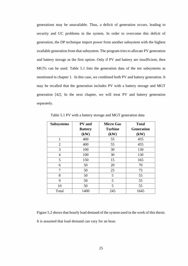
generations may be unavailable. Thus, a deficit of generation occurs, leading to
security and UC problems in the system. In order to overcome this deficit of
generation, the DP technique import power from another subsystem with the highest
available generation from that subsystem. The program tries to allocate PV generation
and battery storage as the first option. Only if PV and battery are insufficient, then
MGTs can be used. Table 5.1 lists the generation data of the ten subsystems as
mentioned in chapter 1. In this case, we combined both PV and battery generation. It
may be recalled that the generation includes PV with a battery storage and MGT
generation [42]. In the next chapter, we will treat PV and battery generation
separately.
Table 5.1 PV with a battery storage and MGT generation data
Subsystems PV and
Battery
(kW)
Micro Gas
Turbine
(kW)
Total
Generation
(kW)
1 400 55 455
2 400 55 455
3 100 30 130
4 100 30 130
5 150 15 165
6 50 20 70
7 50 25 75
8 50 5 55
9 50 5 55
10 50 5 55
Total 1400 245 1645
Figure 5.2 shows that hourly load demand of the system used in the work of this thesis.
It is assumed that load demand can vary for an hour.

26
Figure 5.2 Load demand for a typical day starts from 8 AM onwards.
5.3.2 Operation with no faults
In the system, generation scheduling plays an important role in day to day activity.
The Dynamic Programming schedules the operation of units while satisfying the
constraints. It controls the state of the units (ON or OFF) every hour. The cost of MGT
generation includes fuel cost. But, Photovoltaic generation is using sunlight to
generate electricity for free of cost. Dynamic Programming was used recursively to
look for the best out of all possible solutions by considering both PV and MGT
generation.

27
Figure 5.3 shows the generation of the subsystems in the first hour (8 AM - 9 AM).
The load demand of 700 kW in this hour. Subsystem 1 generates 400 kW of power
from PV. The remaining power must be supplied from the MGT 55 kW. Subsystem
2 generates only 245 kW of power from PV out of its capacity of 400 kW. The DP
technique allocates 55 kW of MGT in Subsystem 1 as shown in Figure 5.3. This is
unfortunate because another 155 kW of PV could be obtained from Subsystem 2. This
technique chooses the best solution by considering the cost of generation and fuel
cost.
Figure 5.3 Power generated in Subsystems 1 and 2 in the first hour (8 AM-9 AM).

28
Figure 5.4 shows the generation of the subsystems in the second hour (9 AM –
10 AM). The load demand increases from 700 kW to 750 kW in this hour.
Subsystem 1 generates 400 kW from PV and 55 kW from MGT. Subsystem 2 now
generates an additional 50 kW from PV totalling 295 kW as shown in Figure 5.4. The
DP technique allocates 55 kW of MGT in Subsystem 1 as before. This is unfortunate
because another 100 kW of PV could be obtained from Subsystem 2. The allocation
of 50 kW from Subsystem 2 is correct.
Figure 5.4 Power generated in Subsystems 1 and 2 in the second hour (9 AM-
10 AM).

29
Figure 5.5 shows the generation of the subsystems in the fifth hour (12 PM – 1 PM).
The load demand of 1000 kW in this hour. Each of Subsystems 1 and 2 generates
400 kW from PV and 55 kW from MGT. Subsystem 5 generates 90 kW from PV as
shown in Figure 5.5. The DP technique allocates 55 kW of MGT in both Subsystems
1 and 2. This is unfortunate because another 100 kW of PV could be obtained from
Subsystems 3 and 4. In spite of this weakness of DP, we continue to test the algorithm
for faulty situation.
Figure 5.5 Power generated in Subsystems 1, 2 and 5 in the fifth hour (12 PM- 1 PM).
Table 5.2 lists the operation with no fault conditions from the first hour (8 AM-9 AM)
to fifth hour (12 PM-1 PM) only. The DP is using MGTs whenever PV generation is
available in most hours such as first, second, third, fourth, fifth hour etc. Here, we

30
mentioned from first (8 AM-9 AM) to fifth hour (12 PM-1 PM) as shown in Table
5.2. In addition, we also mentioned peak load period from tenth (5 PM-6 PM) to
fifteenth hour (10 PM-11 PM) as shown in Table 5.3. The figures for the remaining
hours were presented in Table A.1. These results were obtained for solving the UC
problem by using the DP technique.
Table 5.2 Operation with no fault conditions from first (8 AM-9 AM) to fifth hour
(12 PM-1 PM)
Hour 1
(8 AM-
9 AM)
2
(9 AM-
10 AM)
3
(10 AM-
11 AM)
4
(11 AM-
12 PM)
5
(12 PM-
1 PM) Subsystems
(1-10)
1
PV 400 400 400 400 400
Bat 0 0 0 0 0
MGT 55 55 55 55 55
2
PV 245 295 395 400 400
Bat 0 0 0 0 0
MGT 0 0 0 55 55
3
PV 0 0 0 0 0
Bat 0 0 0 0 0
MGT 0 0 0 0 0
4
PV 0 0 0 0 0
Bat 0 0 0 0 0
MGT 0 0 0 0 0
5
PV 0 0 0 35 85
Bat 0 0 0 0 0
MGT 0 0 0 5 5
6-10
PV 0 0 0 0 0
Bat 0 0 0 0 0
MGT 0 0 0 0 0
Table 5.3 lists the operation with no fault conditions from tenth (5 PM-6 PM) to
fifteenth hour (10 PM-11 PM) which covers the peak load period. Note all that the
DP has allocated MGTs although PVs are available in some subsystems.

31
Table 5.3 Operation with no fault conditions from tenth (5 PM-6 PM) to fifteenth
hour (10 PM-11 PM)
Hour 10
(5 PM-
6 PM)
11
(6 PM-
7 PM)
12
(7 PM-
8 PM)
13
(8 PM-
9 PM)
14
(9 PM-
10 PM)
15
(10 PM-
11 PM) Subsystems
(1-10)
1
PV 100 400 0 0 0 0
Bat 300 0 400 400 400 400
MGT 55 55 55 55 55 55
2
PV 100 400 0 0 0 0
Bat 300 0 400 400 400 400
MGT 55 55 55 55 55 55
3
PV 50 50 0 0 0 0
Bat 50 50 100 100 100 100
MGT 30 30 30 30 30 30
4
PV 50 50 0 0 0 0
Bat 50 50 100 100 100 100
MGT 30 30 30 30 30 30
5
PV 50 0 0 0 0 0
Bat 100 150 150 150 110 30
MGT 15 15 15 15 0 0
6
PV 25 0 0 0 0 0
Bat 0 50 50 45 20 0
MGT 0 30 25 0 0 0
7
PV 0 0 0 0 0 0
Bat 0 25 25 20 0 0
MGT 0 0 0 0 0 0
8
PV 0 0 0 0 0 0
Bat 0 15 50 0 0 0
MGT 0 0 0 0 0 0
9
PV 0 0 0 0 0 0
Bat 0 0 15 0 0 0
MGT 0 0 0 0 0 0
10
PV 0 0 0 0 0 0
Bat 0 0 0 0 0 0
MGT 0 0 0 0 0 0

32
5.3.3 Operation with faults
A fault is applied in Subsystem 5 in the sixth hour (1 PM – 2 PM) when the load
demand is 1100 kW. Each of Subsystems 1 and 2 generates 400 kW of solar and
55 kW of MGT power. Before the fault, Subsystem 4 has been generating 25 kW of
MGT. Subsystem 5 has been generating 150 kW of solar and 15 kW of MGT power
as shown already in Table 5.1. The fault has reduced its PV generation from 150 kW
to 60 kW and MGT generation to 15 kW, the total lost generation being 105 kW.
Figure 5.6 Power generated in Subsystem 1, 2, 4 and 5 in the sixth hour (1 PM-
2 PM).
The DP should recommend adding the highest generation from another subsystem to
replace the lost generation. The power generation in a subsystem has to be generated
power in this order 1, 2, 5, 4, 3, 6, 7, 8, 9 and 10 according to the rating as shown in
Table 5.1. The order of the subsystem is based on the rating of photovoltaic generation

33
from highest to lowest. Since Subsystem 4 has the next highest power generation, it
will generate the remaining power 100 kW of PV and 5 kW of MGT as dictated by
DP as shown in Figure 5.6.
The fault in Subsystem 5 continues to the seventh hour (2 PM - 3 PM). The load
demand in this hour increases from 1100 kW to 1150 kW. Subsystem 1 generates
400 kW of solar and 55 kW of MGT as shown in Figure 5.7. Subsystem 2 generates
400 kW of solar and 5 kW of MGT. Subsystem 3 has been generating 100 kW of solar
and 25 kW of MGT. Subsystem 5 has been generating 150 kW of solar and 15 kW of
MGT power before the fault as shown already in Table 5.1.
Figure 5.7 Power generated in Subsystems 1, 2, 3, 4 and 5 in the seventh hour
(2 PM- 3 PM).
The fault has reduced its PV generation from 150 kW to 30 kW and MGT generation
to 15 kW, the total lost generation being 135 kW. The DP technique should suggest

34
adding Subsystems 3 and 4 to replace the lost generation. Since Subsystems 3 and 4
have the next highest power generation, these subsystems will generate 5 kW of MGT
from Subsystem 3 and 100 kW of PV also 30 kW of MGT from Subsystem 4.
The fault in Subsystem 5 persists in the eighth hour (3 PM- 4 PM). The load demand
increases from 1150 kW to 1200 kW. Each of Subsystems 1 and 2 generates 455 kW
from PV and MGT as shown in Figure 5.8. Subsystem 3 has been generating 100 kW
of solar and 25 kW of MGT. Subsystem 5 has been generating 150 kW of solar and
15 kW of MGT power before the fault. The fault has reduced its PV generation from
150 kW to 30 kW and MGT generation to 15 kW, the total lost generation being
135 kW.
Figure 5.8 Power generated in Subsystems 1, 2, 3, 4 and 5 in the eighth hour (3 PM- 4 PM).

35
To minimize this problem by using the DP technique. This technique should suggest
adding the highest generation from another subsystem to replace the lost generation.
Subsystems 3 and 4 have the next highest power generation. These subsystems will
generate remaining power 5 kW of MGT from Subsystem 3 and 100 kW of PV and
30 kW of MGT from Subsystem 4.
The fault in Subsystem 5 continues to the ninth hour (4 PM – 5 PM) as shown in
Figure 5.9. Each of Subsystems 1 and 2 generates 455 kW from PV and MGT as
before. The load demand increases from 1200 kW to 1300 kW in this hour.
Subsystem 3 has been generating 95 kW of solar power. Subsystem 5 has been
generating 150 kW of solar and 15 kW of MGT power before the fault.
Figure 5.9 Power generated in Subsystems 1, 2, 3, 4, 5 and 6 in the ninth hour
(4 PM- 5 PM).

36
The fault has reduced its PV generation from 150 kW to 105 kW and MGT generation
to 15 kW, the total lost generation being 60 kW. The DP should recommend adding
Subsystems 3 and 6 to replace the lost generation. These subsystems will generate
remaining power 5 kW of PV and 30 kW of MGT from Subsystem 3 also 25 kW of
PV from Subsystem 6.
The fault in Subsystem 5 continues for four hours (from sixth to ninth hour). The fault
is corrected in Subsystem 5 in the tenth hour (5 PM – 6 PM) by using the DP technique
as shown in Figure 5.10.
Figure 5.10 Power generated in Subsystems 1, 2, 3, 4, 5, 6 and 7 in the tenth hour
(5 PM- 6 PM).

37
The load demand in this hour increases from 1300 kW to 1400 kW. Subsystem 5
losses its generation because of fault in previous hours as shown in Figure 5.6 - 5.9.
In this hour, Subsystem 5 generates its maximum capability of 165 kW. Each of
Subsystems 1 and 2 generates 455 kW from PV and MGT. Each of Subsystems 3 and
4 generates 130 kW from PV and MGT. Each of Subsystems 6 and 7 generates 40
kW and 25 kW from PV generation.
Another fault is applied in the fourteenth hour (9 PM – 10 PM) to the same subsystem.
The fault till continues for six hours from the fourteenth hour to the nineteenth hour.
The load demand in this hour is 1300 kW. Each of Subsystems 1 and 2 generates
455 kW from PV and MGT as shown in Figure 5.11.
Figure 5.11 Power generated in Subsystems 1, 2, 3, 4, 5 and 6 in the fourteenth hour
(9 PM-10 PM).

38
Subsystem 4 generates 130 kW of power from PV and MGT. Before the fault,
Subsystem 3 has been generating 100 kW of solar power. Subsystem 5 has been
generating 150 kW of solar and 15 kW of MGT power as shown in Figure 5.10. The
fault has reduced its PV generation from 150 kW to 110 kW and MGT generation to
15 kW, the total lost generation being 55 kW. The DP should recommend adding the
highest available generation from another subsystem to replace the lost generation.
Since Subsystems 3 and 6 have the next highest power generation. These subsystems
will generate 30 kW of MGT from Subsystem 3 also 25 kW of PV from Subsystem 6
as dictated by DP.
The fault in Subsystem 5 continues to the fifteenth hour (10 PM – 11 PM) as shown
in Figure 5.12. The load demand in this hour decreases from 1300 kW to 1200 kW.
Figure 5.12 Power generated in Subsystems 1, 2, 3, 4 and 5 in the fifteenth hour
(10 PM-11 PM).

39
Each of Subsystems 1 and 2 generates 455 kW from PV and MGT. Subsystem 3 has
been generating 100 kW of solar and 25 kW of MGT power. Subsystem 5 has been
generating 150 kW of solar and 15 kW of MGT power before the fault as shown in
Figure 5.10. The fault has reduced its PV generation from 150 kW to 30 kW and MGT
generation to 15 kW, the total lost generation being 135 kW. The DP should suggest
adding the highest generation to replace the lost generation. Since Subsystems 3 and
4 have the next highest power generation. The total lost generation of 135 kW needs
to be replaced by additional generation from Subsystems 3 and 4. Subsystem 3 will
generate an extra 5 kW power from MGT and Subsystem 4 will generate 100 kW
from solar and 30 kW from MGT as dictated by DP.

40
The fault in Subsystem 5 continues to the sixteenth hour (11 PM – 12 AM) as shown
in Figure 5.13. The load demand in this hour decreases from 1200 kW to 1050 kW.
Subsystems 1 generates 455 kW of PV and MGT power. Subsystem 2 has been
generating 400 kW of PV and 30 kW of MGT power. Subsystem 5 has been
generating 150 kW of solar and 15 kW of MGT power before the fault as shown in
Figure 5.10. The fault has reduced its PV generation from 150 kW to 20 kW and
MGT generation to 15 kW, the total lost generation being 145 kW. The DP should
recommend adding the highest available generation from another subsystem to
replace the lost generation. Since Subsystems 2 and 4 have the next highest power
generation. These subsystems will generate 15 kW of MGT from Subsystem 2 and
100 kW of PV and 30 kW of MGT as dictated by DP.
Figure 5.13 Power generated in Subsystems 1, 2, 4 and 5 in the sixteenth hour
(11 PM-12 AM).

41
The fault in Subsystem 5 continues to the seventeenth hour (12 AM -1 AM) as shown
in Figure 5.14. The load demand in this hour decreases from 1050 kW to 1000 kW.
Subsystems 1 generates 455 kW from PV and MGT as before. Subsystem 2 has been
generating 380 kW of solar power. Subsystem 5 has been generating 150 kW of solar
and 15 kW of MGT power before the fault as shown in Figure 5.9. The fault has
reduced its PV generation from 150 kW to 20 kW and MGT generation to 15 kW, the
total lost generation being 145 kW. The DP should recommend adding the highest
available generation from another subsystem. Since Subsystems 2 and 4 have the next
highest power generation. These subsystems will generate 15 kW of solar from
Subsystem 2 and 100 kW of PV and 30 kW of MGT power from Subsystem 4 as
dictated by DP.
Figure 5.14 Power generated in Subsystems 1, 2, 4 and 5 in the seventeenth hour
(12 AM- 1 AM).

42
The fault in Subsystem 5 continues to the eighteenth hour (1 AM - 2 AM) as shown
in Figure 5.15. The load demand in this hour increases from 1000 kW to 1100 kW.
Each of Subsystems 1 and 2 generates 455 kW from PV and MGT. Subsystem 4 has
been generating 25 kW of MGT power. Subsystem 5 has been generating 150 kW of
solar and 15 kW of MGT power before the fault as shown already in Figure 5.10. The
fault has reduced its PV generation from 150 kW to 60 kW and MGT generation to
15 kW, the total lost generation being 105 kW. The DP should recommend adding the
highest available generation from another subsystem to replace the lost generation.
Since Subsystem 4 has the next highest power generation, it will generate 105 kW
from PV and MGT as dictated by DP.
Figure 5.15 Power generated in Subsystems 1, 2, 4 and 5 in the eighteenth hour
(1 AM-2 AM).
43
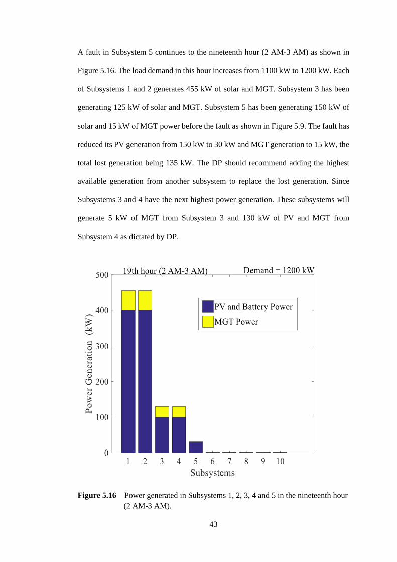
A fault in Subsystem 5 continues to the nineteenth hour (2 AM-3 AM) as shown in
Figure 5.16. The load demand in this hour increases from 1100 kW to 1200 kW. Each
of Subsystems 1 and 2 generates 455 kW of solar and MGT. Subsystem 3 has been
generating 125 kW of solar and MGT. Subsystem 5 has been generating 150 kW of
solar and 15 kW of MGT power before the fault as shown in Figure 5.9. The fault has
reduced its PV generation from 150 kW to 30 kW and MGT generation to 15 kW, the
total lost generation being 135 kW. The DP should recommend adding the highest
available generation from another subsystem to replace the lost generation. Since
Subsystems 3 and 4 have the next highest power generation. These subsystems will
generate 5 kW of MGT from Subsystem 3 and 130 kW of PV and MGT from
Subsystem 4 as dictated by DP.
Figure 5.16 Power generated in Subsystems 1, 2, 3, 4 and 5 in the nineteenth hour
(2 AM-3 AM).

44
A fault is corrected in Subsystem 5 in the twentieth hour (3 AM- 4 AM) by using the
DP technique as shown in Figure 5.17. The load demand in this hour increases from
1200 kW to 1400 kW. Subsystems 1, 2, 3, 4, 6 and 7 generate 455 kW, 455 kW,
130 kW, 130 kW, 45 kW and 20 kW respectively. Subsystem 5 losses its generation
because of fault in previous hours as shown in Figure 5.11-5.16. In this hour,
Subsystem 5 generates its maximum capability of 165 kW.
Figure 5.17 Power generated in Subsystems 1, 2, 3, 4, 5, 6 and 7 in the twentieth
hour (3 AM-4 AM).
There is no fault from the twenty-first hour to the twenty-fourth hour. All the
remaining mentioned hours are operated according to the demand. The fault locations
are detailly mentioned in Table 5.4.
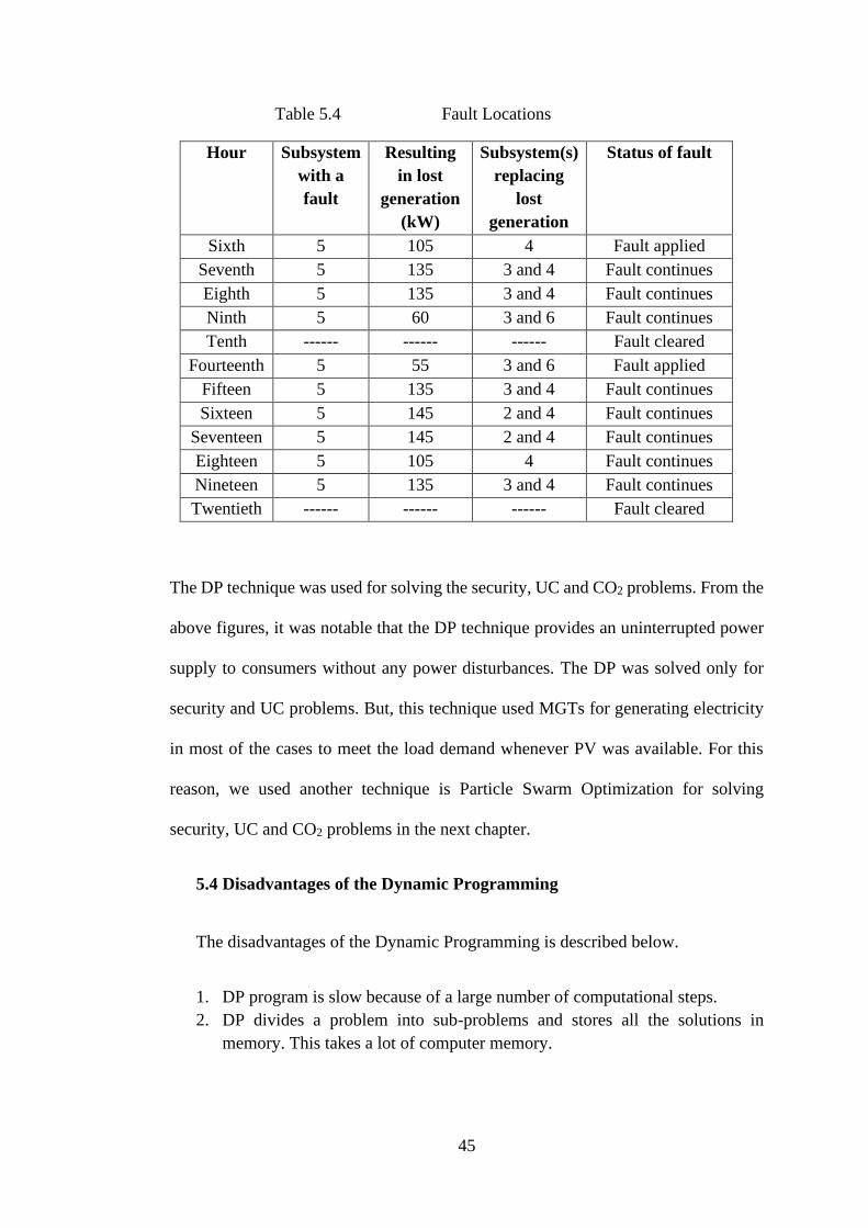
45
Table 5.4 Fault Locations
Hour Subsystem
with a
fault
Resulting
in lost
generation
(kW)
Subsystem(s)
replacing
lost
generation
Status of fault
Sixth 5 105 4 Fault applied
Seventh 5 135 3 and 4 Fault continues
Eighth 5 135 3 and 4 Fault continues
Ninth 5 60 3 and 6 Fault continues
Tenth ------ ------ ------ Fault cleared
Fourteenth 5 55 3 and 6 Fault applied
Fifteen 5 135 3 and 4 Fault continues
Sixteen 5 145 2 and 4 Fault continues
Seventeen 5 145 2 and 4 Fault continues
Eighteen 5 105 4 Fault continues
Nineteen 5 135 3 and 4 Fault continues
Twentieth ------ ------ ------ Fault cleared
The DP technique was used for solving the security, UC and CO2 problems. From the
above figures, it was notable that the DP technique provides an uninterrupted power
supply to consumers without any power disturbances. The DP was solved only for
security and UC problems. But, this technique used MGTs for generating electricity
in most of the cases to meet the load demand whenever PV was available. For this
reason, we used another technique is Particle Swarm Optimization for solving
security, UC and CO2 problems in the next chapter.
5.4 Disadvantages of the Dynamic Programming
The disadvantages of the Dynamic Programming is described below.
1. DP program is slow because of a large number of computational steps.
2. DP divides a problem into sub-problems and stores all the solutions in
memory. This takes a lot of computer memory.

46
Chapter 6
Particle Swarm Optimization
6.1 Introduction
Dynamic Programming (DP) technique can be used for solving security and Unit
Commitment (UC) problems with a single fault as mentioned in Chapter 5. But this
technique has a drawback. It does not consider minimizing the CO2 emissions. It
allocates MGTs even when PV generation is available thus increased the fuel cost.
This is due to the fact that this technique does not always reach a global solution.
Therefore, we should explore some other technique which can cater for security and
UC as well as fuel cost and CO2 emission problems. In addition, we wish to apply
multiple faults simultaneously. Particle Swarm Optimization (PSO) is a population-
based search technique. This technique has the ability to converge quickly for a global
solution. In addition, PSO is suitable for solving the non-differentiable, continues,
non-convex, non-linear, discrete type problems [43].
The PSO approach was first proposed by Russell C. Eberhart and James Kennedy
[44] in the year 1995. This method utilizes swarm intelligence theory which was
inspired by the social behaviour of animals like a school of fish or a flock of birds.
The members of the group communicate among them. For example, when a group of
birds looks for food in a distant location, the members of the group may know all the
possible ways to the probable location of the desired food. But all may not know the
best way to reach the location. If any member of the group can find out the best path
to follow, the remaining members in the group are intimated so that they can follow
swiftly to the desired location. Birds in the group communicate with each other with
their movements. Their movement consists of two behaviours like balancing and

47
opposing. In balancing behaviour, birds adjust their movements to try to reach the
food location and protect themselves from hunters. The birds need to avoid collisions
within the group due to opposing behaviour [45].
In this technique, each member of the population in the search space is called a
particle, individual or agent. Each agent has its own velocities and fitness values. The
PSO method is initialized with a group of agents moving in random directions to
search for the global solution for a problem. An agent can communicate with other
members in the same group to find out the best position of itself. The terms used to
explain the PSO are defined below:
1. Agent (particle, individual): Each member in the group (swarm);
2. Swarm: The group of the agents itself;
3. Position/Location: Each agent has n-dimensional coordinates, which
represents an accurate solution for the problem;
4. Generation: Every iteration of the optimization procedure.
5. Vmax : The maximum velocity value permitted in a direction;
6. Fitness Function: This function provides the interface between the physical
and optimization problems;
7. Particle Best: The location in the parameter space of the best fitness value
returned to an agent;
8. Global Best: The location in the parameter space of the best fitness value
returned to the swarm.
6.1.1 Global best algorithm
In this technique, each individual agent, i, has a current velocity, vi, best location,
pbesti, and a current location, xi. The global best location, gbest, is for the entire swarm.
In each iteration, the agent best and global best values are updated [46]. The algorithm
for updating their values are given in Equation 6.1 below.
=+1t
ipbest t
ipbest,
t
i
t
i pbestxf )( (6.1)
where

48
t
ipbest : the best agent location of each agent, i , at the time step, t ,
t
ix : current location of each agent, i at the time step, t .
The global best location at time step, t, is given by Equation 6.2.
}min{ t
ipbestgbest = (6.2)
PSO technique consists of one main operator in the velocity equation. Each agent also
carries a memory. The velocity provides the search directions for each agent and
needs to be updated for each iteration. Each agent tries to change its location by using
the following information: (1) current locations of agents, (2) distance between the
global best and current locations, (3) current velocities and (4) distance between the
agent best and current locations.
The velocity of an agent, i, can be modified by using Equation 6.3.
][][ 2211
1 t
ij
t
j
t
ij
t
i
t
j
t
ij
t
ij xgbestrcxpbestrcvv −+−+=+
(6.3)
Where
t
ijv : the velocity vector of an agent, i , in dimension, j , at time step, t ,
t
ipbest : the personal best position of an agent, i , at time step, t , already
mentioned in Equation 6.1,
t
ijx : the location vector of agent, i , in dimension, j , at time step, t ,
gbest : the global solution of the entire swarm already mentioned in
Equation 6.2,
21,cc : positive acceleration constants,
21,rr : random numbers in the range of [0,1].
6.2 Parameters of PSO
The PSO uses a few parameters in addition to the two (velocity, global best) we
mentioned above. These parameters and their values have a large impact on the

49
efficiency of the PSO in an optimization problem. The parameters are (1) swarm size,
(2) iterations, (3) velocity, (4) acceleration coefficients (5) neighbourhood topologies
and (6) inertia weight etc.
6.2.1 Swarm size
Swarm size is the number of agents in the swarm. A swarm generates more search
space to be enclosed per iteration. But swarm size may increase the required time and
the computational complexity of each iteration to find an optimization result. From a
number of studies, it was revealed that a swarm size of 20 to 60 is suitable for a global
solution in most cases.
6.2.2 Velocity components
Like other components, the velocity components are also updated for each agent.
There are three main terms for agent’s velocity in Equation 6.3. Such as inertia
component, cognitive component and social component.
1. The inertia component, t
ijv , gives detailed information of the previous
memory flight direction. This component prevents any change to the agents’
direction.
2. The cognitive component, ][ 111
t
j
t
i
t
j xpbestrc − , measures the agents’
performance related to past performance.
3. The social component, ][22
t
ij
t
j xgbestrc − , measures the agents’ performance
related to a swarm. This component affects each agents’ flight towards the
best location found by its neighbours.
6.2.3 Iteration
A low number of iterations can stop the search process prematurely, whereas a large
number of iterations will involve a long time and increased computational complexity

50
[47]. The number of iterations required for obtaining a good result depends on the
problem.
6.2.4 Acceleration coefficients
The acceleration coefficients, c1, and, c2, together with the random numbers, r1, and,
r2, maintain the influence of the social and cognitive components of the agents’
velocity. The constant, c1, expresses how much confidence an agent has in itself.
Similarly, the constant, c2 expresses how much confidence an agent has on its
neighbours. There are a few properties of the two constants, c1, and, c2.
1. When (c1 > 0) and (c2 = 0), all agents are independent. The velocity
Equation 6.3 now reduces to.
][11
1 t
ij
t
i
t
j
t
ij
t
ij xpbestrcvv −+=+ (6.4)
2. On the other hand, when (c1 = 0) and (c2 > 0), all agents are attached to a single
point in the swarm. The velocity equation can be updated as follows.
)(22
1 t
ij
t
j
t
ij
t
ij xgbestrcvv −+=+ (6.5)
3. When (c1 = c2 = 0), all agents are continuing their flying towards the current
location until they hit the space boundary. Hence, the velocity Equation 6.3 is
calculated as follows.
t
ij
t
ij vv =+1 (6.6)
4. When (c1 = c2), all agents are attached to the, pbestit, and, gbest.
5. When (c1 >> c2), each individual agent is influenced by its agent’s location
which results in wandering.
6. When (c2 >> c1), all agents are influenced by the swarm location, which causes
all agents to run continuously without stopping.
Generally, the wrong initialization of constants may lead to cyclic and divergent
behaviour. Researchers observed that the two constants must be c1 = c2 = 2 [48].
6.2.5 Neighbourhood topologies
The PSO has social interaction among the agents’ in the swarm. Agents communicate
with others by exchanging information (current location and velocity of an agent) to

51
obtain the global solution in the swarm [48]. It influences agents’ movement with this
information. If an agent in the swarm finds a global solution, remaining agents follow
this agent. The performance of the agents is determined by the agents’ neighbourhood.
A neighbourhood should be defined for each agent. This approach leads to faster
convergence because of the agent’s move towards a search space.
6.2.6 Inertia weight
The inertia weight, w, was introduced by Eberhart and Shi in the year 1999 [49]. The
inertia weight is multiplied by the velocity of the previous time step. Hence, the
velocity Equation 6.3 is modified as follows,
][][ 2211
1 t
ij
t
j
t
ij
t
i
t
j
t
ij
t
ij xgbestrcxpbestrcwvv −+−+=+ (6.7)
where
w : the inertia weight,
t
ijv , t
ipbest , t
ijx , gbest , 21,cc , 21,rr as defined in Equation 6.3.
If the inertia weight is much less than unity, rapid changes of direction occur. If inertia
weight is negligible, all agents will move without having the knowledge of the
previous velocity in each step. If inertia weight is greater than or equal to unity, the
velocities of agents’ increase and agents’ may change their direction to move back for
an optimal solution.
Generally, if inertia weight is high, all agents can move freely in the space at the initial
stage and minimize overall time. But, if inertia weight is low, agents have produced
good results for solving optimization problems. According to the velocity equation,
the inertia weight is set as follows [50].

52
tt
wwwwt
−−=+
max
minmaxmax
1
(6.8)
where
maxw : maximum values of inertia weight,
minw : minimum values of inertia weight,
t : the current number of iterations,
maxt : the maximum number of iterations.
The step by step procedure of using PSO algorithm for solving a problem is as
follows.
1. Initialize the agents by assigning a random position in the search space.
2. Find out the agent best position and evaluate the fitness function for each
agent.
3. For each agent, compare the agent’s fitness value with its agent best.
4. Identify the agent which has the best fitness value. The best fitness value is
identified as a global best.
5. Update the position and velocity of each agent using Equations (6.3) and (6.7).
6. Repeat steps 2-5 till to stop criteria is to meet (for example, when it reaches
the maximum number of iterations).
The PSO parameters used for the simulation are shown in Table 6.1 below.
Table 6.1 Optimal parameter settings for the PSO
Parameters Values
Population size 40
Number of iterations 100
Cognitive constant, c1 2
Social constant, c2 2
Inertia weight, w 0.3-0.95

53
6.3 Advantages of the Particle Swarm Optimization
The advantages of the PSO as follows [51].
1. PSO algorithm is easy to implement. It is a derivative-free algorithm.
2. PSO has a limited number of parameters compared to other traditional
methods.
3. PSO involves simple calculations.
4. PSO has less computational time.
5. This algorithm does not involve any mathematical derivations.
6.4 Micro Gas Turbines
The characteristics of MGT must be expressed by fuel consumption and CO2
emissions [52].
6.4.1 Fuel consumption
MGT fuel consumption can be formulated by using load characteristics [53]. The
efficiency between the output of electrical energy kMGTE _( in )electrickWh and thermal
energy is supplied to the combustion chamber of MGT kMGTT _( in )thermalkWh
mathematically expressed as:
kMGT
kMGT
kT
E
_
_=
(6.9)
where
kMGTE _ : the electrical energy output from MGT,
k : generating units,
kMGTT _ : thermal energy from MGT.
The efficiency of MGT is a non-linear function, which depends on the load ratio.

54
MAXkMGT
kMGT
kP
tPt
__
_ )()( =
(6.10)
where
kMGTP _ : generated electrical power by MGT,
: the energy efficiency for load,
MAXkMGTP __ : the rated power of MGT.
Based on Equations 6.9 and 6.10 the MGT fuel consumption is calculated for every
one-hour interval sec)3600( = with constant power output.
k
MAXkMGTk
kMGT
PttT
__
_
)()( = (6.11)
where
kMGTT _ : the MGT thermal energy,
: time interval for every one-hour interval.
The fuel cost of MGT is obtained from Equation 6.12 as a function of the electrical
power generation by using MGT, PMGT_k(t).
))(( _ tPfR kMGTk = (6.12)
where
kMGTP _ : the electrical power generation of MGT,
kR : the fuel cost of MGT.
6.4.2 Carbon dioxide emissions
The CO2 emissions are calculated by applying several weights to the pollutant gases.
The masses of three exhaust gases Carbon monoxide (CO), Nitrogen Oxide (NOx)

55
and Carbon Dioxide (CO2) are considered in g/kWh a mathematical function of
generated power by MGT [54]. By considering the emission factor, y , is equal to
202 g/kWh referred to the thermal energy, E, is generated by burning the fuel as input
to the MGT. This was applied to the CO2 emissions as follows,
MAXkMGTkykMGTyy PttEtN ___ )()()( == (6.13)
where
: emission factor (specific emission) of gas,
)/( electricy kWhmg : specific emission for y or CO2 pollutant gas,
yN : the mass of emissions,
: the energy efficiency for load,
: time interval for every one-hour.
In order to calculate the CO2 emissions, 298 grams of CO2 is equivalent to 1 gram of
NOx and 3 grams of CO2 to 1 gram of CO [55]. By using these Equations 6.11, 6.12
and 6.13, the efficiency of the MGT is calculated.
6.5 Simulation results
6.5.1 Generation data
In this thesis, a fault was applied, identified and cleared by the PSO. It was assumed
that a faulted subsystem will lose all its generation and the system will need to look
for generation from other healthy subsystems. Loss of generation in the faulted
subsystems leads to security and UC problems. Batteries can be used during night
time and if PVs are insufficient in day time also. The detailed information about
generating data of the ten subsystems and hourly load demand for a typical day was
mentioned in chapter 5.

56
Figure 6.1 Generation data for PV, battery and MGTs in the subsystems.
Figure 6.1 shows the generation data for PV, battery and MGTs data for ten
subsystems. It is shown in this figure that PV generation and battery have the same
power rating in all subsystems [41]. This information was already provided in
Table 5.1 before. Subsystems 1, 2, 3, 4 and 5 have considered the highest PV and
battery capacity. PVs are only available in the day time to supply the required amount
of power. But, batteries and MGTs are used at night time. It is also assumed that
batteries will be fully charged during day time.

57
6.5.2 Operation with no fault
Figure 6.2 shows the generation of the subsystems in the first hour (8 AM - 9 AM).
The load demand for this hour is 700 kW. Subsystems 1 and 2 are called upon to
generate power by using only PV systems. Subsystem 1 generates 395 kW of solar
power and obtains 5 kW from battery. Subsystem 2 generates 295 kW of solar power
and obtains 5 kW from battery.
Figure 6.2 Subsystems 1 and 2 are committed in the first hour (8 AM-9 AM).

58
Figure 6.3 shows the generation of the subsystems in the second hour (9 AM -
10 AM). The load demand for this hour is 750 kW. Subsystems 1 generates 395 kW
of solar power and obtains 5 kW from battery. Subsystem 2 generates 345 kW of solar
and obtains 5 kW from battery. The use of 5 kW from battery is an arbitrary one in
both subsystems. The larger amount of battery power can be utilised if necessary.
There is no fault in the first and second hours.
Figure 6.3 Subsystems 1 and 2 are committed in the second hour (9 AM-10 AM).

59
6.5.3 Operation with fault
Before the fault, each of Subsystems 1 and 2 supplies 200 kW of solar, 200 kW from
battery and 55 kW of MGT in the tenth hour (5 PM – 6 PM) when the load demand
is 1400 kW. Each of Subsystems 3 and 4 supplies 30 kW of solar, 70 kW from battery
and 30 kW of MGT. Subsystem 5 supplies 40 kW from solar and 110 kW from
battery. Subsystems 6 and 7 generate 50 kW and 30 kW of solar as shown in
Figure 6.4.
Figure 6.4 Subsystems 1, 2, 3, 4, 5, 6 and 7 are committed in the tenth hour (5 PM-
6 PM) before the fault.

60
A fault is applied in Subsystem 6 in the tenth hour. Before the fault, Subsystem 6
generates 50 kW of PV generation as shown in Figure 6.4. The fault has reduced its
generation from 50 kW to 0 kW, the total lost generation is 50 kW. The PSO should
recommend adding the next available generation from another subsystem to replace
the lost generation. Subsystems 7 and 8 have the next available generation. These
subsystems will generate 50 kW of solar power. Subsystem 7 has increased its PV
generation from 30 kW to 50 kW. Subsystem 8 generate 30 kW of solar power as
shown in Figure 6.5.
Figure 6.5 Subsystems 7 and 8 have to generate their output to make up for the loss
of generation in Subsystem 6 in the tenth hour (5 PM-6 PM).

61
Before the fault, each of Subsystems 1 and 2 supplies 400 kW from battery and
55 kW of MGT in the fourteenth hour (9 PM – 10 PM) when the load demand is
1300 kW. Subsystems 3 and 4 supply 100 kW from battery. Subsystems 5 and 6
obtain 150 kW and 40 kW from battery as shown in Figure 6.6.
Figure 6.6 Subsystems 1, 2, 3, 4, 5 and 6 are committed in the fourteenth hour
(9 PM-10 PM) before the fault.

62
Figure 6.7 shows that another different fault is applied in Subsystem 4 in the
fourteenth hour. Each of Subsystems 1 and 2 supplies 400 kW from battery and
55 kW of MGT. Subsystems 3, 5 and 6 obtain 100 kW, 150 kW and 50 kW from
battery. Before the fault, Subsystem 4 obtains 100 kW from battery as shown in
Figure 6.6. The fault has reduced its generation from 100 kW to 0 kW, the total lost
generation is 100 kW. The PSO should recommend adding the next available
generation from another subsystem to replace the lost generation. Subsystems 7, 8
and 9 have the next available generation. These subsystems will obtain 100 kW from
battery. Subsystems 7, 8 and 9 obtain 50 kW, 40 kW and 10 kW from battery.
Figure 6.7 Subsystems 7, 8 and 9 have to generate their output to make up for the
loss of generation in Subsystem 4 in the fourteenth hour (9 PM-10 PM).

63
Before the fault, each of Subsystems 1 and 2 obtains 400 kW from battery in the
seventeenth hour (12 AM – 1 AM) when the load demand is 1000 kW. Each of
Subsystems 3 and 5 obtains 50 kW from battery. Subsystem 4 supplies 100 kW from
battery as shown in Figure 6.8.
Figure 6.8 Subsystems 1, 2, 3, 4 and 5 are committed in the seventeenth hour
(12 AM-1 AM) before the fault.

64
Figure 6.9 shows that another different fault is applied in Subsystem 5 in the
seventeenth hour. Before the fault, Subsystem 5 obtains 50 kW from battery as shown
in Figure 6.8. The fault has reduced its generation from 50 kW to 0 kW, the total lost
generation is 50 kW. The PSO should recommend adding the next available
generation from another subsystem to replace the lost generation. Subsystem 3 has
the next available generation. Subsystem 3 has increased its battery from 50 kW to
100 kW from battery. For economic and environmental reasons, PV and battery
should be used as a first option. MGT will only be used when PV and battery fail to
generate adequate power.
Figure 6.9 Subsystem 3 has to increase its output to make up for the loss of
generation in Subsystem 5 in the seventeenth hour (12 AM-1 AM).

65
Before the fault, each of Subsystems 1 and 2 supplies 400 kW from battery and
55 kW of MGT in the twenty-first hour (4 AM – 5 AM) when the load demand is
1300 kW. Each of Subsystems 3 and 4 supplies 100 kW from battery. Subsystems 5
and 6 supply 150 kW and 40 kW from battery as shown in Figure 6.10.
Figure 6.10 Subsystems 1, 2, 3, 4, 5 and 6 are committed in the twenty-first hour
(4 AM-5 AM) before the fault.

66
Figure 6.11 shows that another different fault is applied in Subsystem 3. Each of
Subsystems 1 and 2 supplies 400 kW from battery and 55 kW from MGT. Subsystems
4, 5 and 6 supply 100 kW, 150 kW and 50 kW from battery. Before the fault,
Subsystem 3 supply 100 kW from battery as shown in Figure 6.10. The fault has
reduced its generation from 100 kW to 0 kW, the total lost generation is 100 kW. The
PSO should recommend adding the next available generation from another subsystem
to replace the lost generation. Subsystems 7, 8 and 9 have the next available
generation. These subsystems obtain 50 kW, 30 kW and 20 kW from battery.
Figure 6.11 Subsystems 7, 8 and 9 have to generate their output to make up for the
loss of generation in Subsystem 3 in the twenty-first hour (4 AM-
5 AM).

67
The fault locations are detailly mentioned in Table 6.2.
Table 6.2 Fault Locations for a single fault
Fault
Duration
Subsystem
with a
fault
Resulting
in lost
generation
(kW)
Subsystem(s)
replacing
lost
generation
Status of fault
5 PM-6 PM 6 50 7 and 8 Fault applied
9 PM-10 PM 4 100 7, 8 and 9 Fault applied
12 AM-1 AM 5 50 3 Fault applied
4 AM-5 AM 3 100 7, 8 and 9 Fault applied
The PSO technique was used for solving the security and UC problems. This
technique was effectively solved both problems and used only PV generation in most
of the cases than MGT generation. Next, we then applied two simultaneous random
faults in two different subsystems.
6.5.4 Case studies
In the studies for this project, the following cases were considered. The system will
be operated in stand-alone mode.
Case 1: Faults applied to Subsystems 3 and 4 in the seventh hour.
Case 2: Faults applied to Subsystems 6 and 7 in the thirteenth hour.
Case 3: Faults applied to Subsystems 3 and 5 in the sixteenth hour.
Case 4: Faults applied to Subsystems 4 and 5 in the seventeenth hour.
Case 5: Faults applied to Subsystems 5 and 6 in the twenty-second hour.
From 1 to 6 hours, all the subsystems are operating in normal condition. Note that we
did not apply faults in Subsystems 1 and 2. Because these subsystems contain the
highest PV generation and battery capacity. If a fault occurs in Subsystems 1 or 2 then
these subsystems will fail to generate power at all. The remaining subsystems did not
generate the required amount of power to replace the lost generation. Because

68
available subsystems did not have that much of capacity to generate power. The below
case studies are faulty subsystems.
Case 1: Before faults, Subsystem 1 supplies 395 kW of solar, 5 kW from battery and
55 kW of MGT power in the seventh hour (2 PM-3 PM). The load demand in this
hour is 1150 kW. Subsystem 2 supplies 395 kW of solar, 5 kW from battery and 5 kW
of MGT power. Subsystem 5 generates 90 kW of solar as shown in Figure 6.12.
Figure 6.12 Subsystems 1, 2, 3, 4 and 5 are committed in the seventh hour (2 PM-
3 PM) before faults.

69
Faults are applied randomly to the Subsystems 3 and 4 in the seventh hour. Before
faults, Each of Subsystems 3 and 4 generates 100 kW of PV generation as shown in
Figure 6.12. The faults have reduced their generation from 100 kW to 0 kW in two
subsystems, the total lost generation of two subsystems is 200 kW. This deficit of
power is compensated by other subsystems selected by the PSO as shown in
Figure 6.13. The PSO should suggest adding the next PV generation from another
healthy subsystem. Since Subsystems 5, 6, 7, 8 and 9 have the next available
generation. These subsystems will generate 200 kW of solar power as dictated by
PSO. Subsystem 5 has increased its PV generation from 90 kW to 150 kW. The
remaining subsystems will generate 50 kW, 50 kW, 25 kW and 15 kW respectively.
Figure 6.13 Subsystems 5, 6, 7, 8 and 9 have to generate their output to make up for
the loss of generation in Subsystems 3 and 4 in the seventh hour (2 PM-
3 PM).

70
Case 2: Before faults, Each of Subsystems 1 and 2 supplies 400 kW from battery and
55 kW of MGT power in the thirteenth hour (8 PM - 9 PM) during night time. The
load demand in this hour is 1400 kW. Each of Subsystems 3 and 4 supplies 100 kW
from battery and 30 kW of MGT. Subsystem 5 obtains 150 kW from battery as shown
in Figure 6.14. Note that the MGT is used in some of the Subsystems 1, 2, 3 and 4.
Because of PV and battery are not available to generate the required power then MGT
will be used in this hour.
Figure 6.14 Subsystems 1, 2, 3, 4, 5, 6 and 7 are committed in the thirteenth hour
(8 PM- 9 PM) before faults.
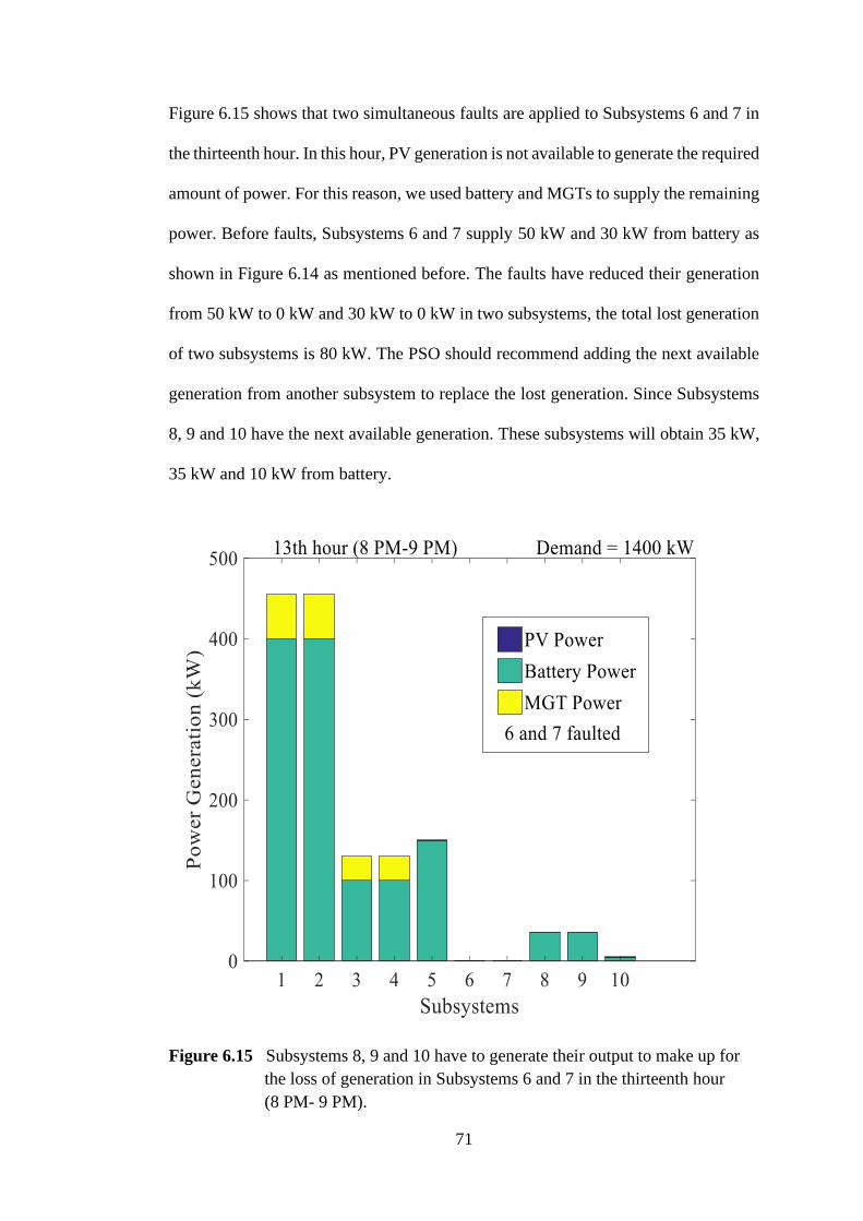
71
Figure 6.15 shows that two simultaneous faults are applied to Subsystems 6 and 7 in
the thirteenth hour. In this hour, PV generation is not available to generate the required
amount of power. For this reason, we used battery and MGTs to supply the remaining
power. Before faults, Subsystems 6 and 7 supply 50 kW and 30 kW from battery as
shown in Figure 6.14 as mentioned before. The faults have reduced their generation
from 50 kW to 0 kW and 30 kW to 0 kW in two subsystems, the total lost generation
of two subsystems is 80 kW. The PSO should recommend adding the next available
generation from another subsystem to replace the lost generation. Since Subsystems
8, 9 and 10 have the next available generation. These subsystems will obtain 35 kW,
35 kW and 10 kW from battery.
Figure 6.15 Subsystems 8, 9 and 10 have to generate their output to make up for
the loss of generation in Subsystems 6 and 7 in the thirteenth hour
(8 PM- 9 PM).
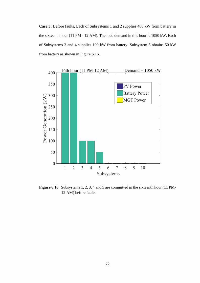
72
Case 3: Before faults, Each of Subsystems 1 and 2 supplies 400 kW from battery in
the sixteenth hour (11 PM - 12 AM). The load demand in this hour is 1050 kW. Each
of Subsystems 3 and 4 supplies 100 kW from battery. Subsystem 5 obtains 50 kW
from battery as shown in Figure 6.16.
Figure 6.16 Subsystems 1, 2, 3, 4 and 5 are committed in the sixteenth hour (11 PM-
12 AM) before faults.

73
Two simultaneous random faults are applied to Subsystems 3 and 5 in the sixteenth
hour. Subsystem 4 obtains 100 kW from battery. Before faults, Subsystems 3 and 5
obtain 100 kW and 50 kW from battery as shown in Figure 6.16. The faults have
reduced their generation from 100 kW to 0 kW and 50 kW to 0 kW in two subsystems,
the total lost generation of two subsystems is 150 kW. The PSO should recommend
adding the next available generation from another subsystem to replace the lost
generation. Since Subsystems 6, 7, 8 and 9 have the next available generation. These
subsystems will obtain 50 kW, 50 kW, 40 kW and 10 kW from battery as shown in
Figure 6.17.
Figure 6.17 Subsystems 6, 7, 8 and 9 have to generate their output to make up for
the loss of generation in Subsystems 3 and 5 in the sixteenth hour
(11 PM-12 AM).

74
Case 4: Before faults, Each of Subsystems 1 and 2 supplies 400 kW from battery in
the seventeenth hour (12 AM-1 AM). The load demand in this hour is 1000 kW. Each
of Subsystems 3 and 5 supplies 50 kW from battery. Subsystem 4 obtains 100 kW
from battery as shown in Figure 6.18.
Figure 6.18 Subsystems 1, 2, 3, 4 and 5 are committed in the seventeenth hour
(12 AM-1 AM) before faults.

75
Two different faults are applied to Subsystems 4 and 5 in the seventeenth hour as
shown in Figure 6.19. Before faults, Subsystems 4 and 5 obtain 100 kW and 50 kW
from battery as shown in Figure 6.18. The faults have reduced their generation from
100 kW to 0 kW and 50 kW to 0 kW in two subsystems, the total lost generation of
two subsystems is 150 kW. The PSO should recommend adding the next available
generation from another subsystem to replace the lost generation. Since
Subsystems 3, 6 and 7 have the next available generation. Subsystem 3 has increased
its generation from 50 kW to 100 kW. The remaining subsystems will supply 50 kW,
50 kW respectively.
Figure 6.19 Subsystems 3, 6 and 7 have to generate their output to make up for
the loss of generation in Subsystems 4 and 5 in the seventeenth hour
(12 AM-1 AM).

76
Case 5: Before faults, Each of Subsystems 1 and 2 supplies 400 kW from battery in
the twenty-second hour (5 AM-6 AM). The load demand in this hour is 1100 kW.
Each of Subsystems 3 and 4 supplies 100 kW from battery. Subsystem 5 obtains
100 kW from battery as shown in Figure 6.20.
Figure 6.20 Subsystems 1, 2, 3, 4 and 5 are committed in the twenty-second hour
(5 AM-6 AM) before faults.

77
Faults are applied to Subsystems 5 and 6 in the twenty-second hour as shown in
Figure 6.21. Before faults, Subsystems 5 and 6 obtain 100 kW and 0 kW from battery
as shown in Figure 6.20. In this figure, Subsystem 6 has not generated any power.
The faults have reduced their generation from 100 kW to 0 kW and 0 kW in two
subsystems, the total lost generation of two subsystems is 100 kW. The PSO should
recommend adding the next available generation from another subsystem to
compensate for a deficit power. Generally, Subsystem 6 has to generate loss of
generation but, this subsystem was faulted. For this reason, Subsystems 7, 8 and 9
have the next available generation. These subsystems will supply 50 kW, 40 kW and
10 kW from battery.
Figure 6.21 Subsystems 7, 8 and 9 have to generate their output to make up for
the loss of generation in Subsystems 5 and 6 in the twenty-second hour
(5 AM- 6 AM).

78
In the above-mentioned cases, the PSO technique was used for solving security and
UC problems. This technique used only for PV generation in most of the cases and
tried to avoid MGTs as much as possible in order to reduce CO2 emissions.
Table 6.3 represents the different fault locations and committed subsystems for
solving security and UC problems in the generation system.
Table 6.3 Faults locations for various cases
Cases Faulty
subsystem
Fault
duration
Generation
loss
(kW)
Subsystems
replacing lost
generation
1 3 and 4 2 PM-3 PM 200 5, 6, 7, 8 and 9
2 6 and 7 8 PM-9 PM 80 8, 9 and 10
3 3 and 5 11 PM-12 AM 150 6, 7, 8 and 9
4 4 and 5 12 AM-1 AM 150 3, 6 and 7
5 5 and 6 5 AM-6 AM 100 7, 8 and 9
Figure 6.22 Total cost of generation.

79
Note that PSO commits PV as long as available. Figure 6.22 shows the total cost
analysis of both PV and MGT generation for a typical day. It was assumed that the
cost of PV generation in Australia is 0.016 AUD per kWh and the cost of MGTs
generation is 0.024 AUD per kWh. By observing this graph, the DP technique was
utilised more MGTs generation than PV generation. For this reason, the total cost will
be high while considering the fuel cost in MGTs. The PSO technique was utilised
more PV generation than MGT generation. Because of this reason, the total cost will
be low.
Table 6.4 lists the PSO performance results from first (8 AM- 9 AM) to fifth hour
(12 PM-1 PM) only. If PV and battery are inadequate then MGTs will be used in
some hours such as ninth, tenth, eleventh, twelfth, thirteenth, fourteenth hour etc as
shown in Table 6.5. In these hours, PSO used available PV generation from other
subsystems on required. Here, we mentioned from the first hour (8 AM- 9 AM) to
fifth hour (12 PM-1 PM) as shown in Table 6.4. In addition, we also mentioned the
peak load period from the tenth hour (5 PM-6 PM) to fifteenth hour (10 PM-11 PM)
as shown in Table 6.5. The figures for the remaining hours were presented in
Table A.2. These results were obtained for solving the UC problem by using the PSO
technique.

80
Table 6.4 PSO performance results from first (8 AM- 9 AM) to fifth hour
(12 PM-1 PM)
Hour 1
(8 AM-
9 AM)
2
(9 AM-
10 AM)
3
(10 AM-
11 AM)
4
(11 AM-
12 PM)
5
(12 PM-
1 PM) Subsystems
(1-10)
1
PV 395 395 395 395 400
Bat 5 5 5 5 0
MGT 0 0 0 0 0
2
PV 295 345 395 395 400
Bat 5 5 5 5 0
MGT 0 0 0 0 0
3
PV 0 0 45 0 50
Bat 0 0 5 0 0
MGT 0 0 0 0 0
4
PV 0 0 0 100 0
Bat 0 0 0 0 0
MGT 0 0 0 0 0
5
PV 0 0 0 0 150
Bat 0 0 0 0 0
MGT 0 0 0 0 0
6-10
PV 0 0 0 50 0
Bat 0 0 0 0 0
MGT 0 0 0 0 0
Table 6.5 lists the PSO performance results which covers the peak load period from
the tenth hour (5 PM-6 PM) to the fifteenth hour (10 PM-11 PM).

81
Table 6.5 PSO performance results from tenth (5 PM-6 PM) to fifteenth hour
(10 PM-11 PM)
Hour 10
(5 PM-
6 PM)
11
(6 PM-
7 PM)
12
(7 PM-
8 PM)
13
(8 PM-
9 PM)
14
(9 PM-
10 PM)
15
(10 PM-
11 PM) Subsystems
(1-10)
1
PV 200 150 100 0 0 0
Bat 200 250 300 400 400 400
MGT 55 55 55 55 55 55
2
PV 200 150 100 0 0 0
Bat 200 250 300 400 400 400
MGT 55 55 55 55 55 55
3
PV 30 30 10 0 0 0
Bat 70 70 90 100 100 100
MGT 30 30 30 30 0 0
4
PV 30 30 10 0 0 0
Bat 70 70 90 100 100 100
MGT 30 30 30 30 0 0
5
PV 50 40 40 0 0 0
Bat 100 110 110 150 150 90
MGT 0 0 0 0 0 0
6
PV 50 20 20 0 0 0
Bat 0 30 30 50 40 0
MGT 0 0 0 0 0 0
7
PV 30 20 20 0 0 0
Bat 0 30 30 30 0 0
MGT 0 0 0 0 0 0
8
PV 0 30 20 0 0 0
Bat 0 0 30 0 0 0
MGT 0 0 0 0 0 0
9
PV 0 0 0 0 0 0
Bat 0 0 30 0 0 0
MGT 0 0 0 0 0 0
10
PV 0 0 0 0 0 0
Bat 0 0 0 0 0 0
MGT 0 0 0 0 0 0

82
The trend of finding the optimum solution is revealed in Table 6.4 - 6.5. The obtained
results demonstrate that the PSO technique was effectively solved the UC problem
than the DP technique.

83
Chapter 7
Conclusions and future works
Chapter 7
In this chapter, the conclusions of the work are presented. In addition, any scope of
future work in the area is discussed.
7.1 Conclusions
In this thesis, two optimization techniques viz, Dynamic Programming and Particle
Swarm Optimization were used for solving security and Unit Commitment problems
of a small isolated system. The system consisted of ten different subsystems each
containing a Renewable Energy Source (Photovoltaic) and a Non-Renewable Energy
Source (Micro Gas Turbine). A single fault was applied to one of the subsystems at
different hours of the day. The Dynamic Programming technique was used to the
system to identify the faulted subsystem and recommend commitment of adequate
generation from another subsystem in order to meet the load requirement of the
system. The Dynamic Programming was able to commit adequate generation from
another subsystem. Unfortunately, this technique committed Micro Gas Turbines
even though Photovoltaic generation was available in the healthy subsystems.
Although, this technique solved the security and Unit Commitment problems
satisfactorily, it failed to satisfy the CO2 emissions constraints because it used Micro
Gas Turbines.
Next, the Particle Swarm Optimization technique was used for solving the same
problem i.e. security and Unit Commitment problems after a fault. As with the

84
Dynamic Programming Technique, we applied a single fault to one of the subsystems,
this time randomly. This technique was also able to identify the faulted subsystem
and committed required amount of power from another subsystem. It is noted that this
technique committed Photovoltaic generation when available. We repeated this test
for different locations of the fault. In all the cases, this technique was successful in
identifying the fault location and committing the required amount of power from
another subsystem. The important thing is that the Particle Swarm Optimization
technique did not commit Micro Gas Turbines as long as Photovoltaic generation was
available. Then two random faults were applied to two different subsystems
simultaneously. We repeated this for a number of cases faults occurring at different
hours. In all the cases, the Particle Swarm Optimization technique correctly identified
both the faulted subsystems and recommended commitment of the Photovoltaic
generation when available. Micro Gas Turbines were committed only when all
available Photovoltaic generation and battery were already committed. Thus, both
techniques are good for solving security and Unit Commitment problems, but the
Dynamic Programming technique used Micro Gas Turbines unnecessarily involving
generation of CO2 emissions. We, therefore, conclude that the Particle Swarm
Optimization technique solved successfully both the security and Unit Commitment
problems along with minimization of the CO2 emissions. This is a clear advantage of
the Particle Swarm Optimization technique over the Dynamic Programming
technique.
7.2 Future Scope
The work reported in this thesis can be extended by incorporating the fuel cells instead
of MGTs, thus automatically minimizing CO2 emissions. The Particle Swarm

85
Optimization can be used for solving Unit Commitment and security problems in
larger systems as well. This work can also be extended to hybrid techniques such as
Simulated Annealing, Ant Colony Optimization, Harmony Search, Evolutionary
Computation etc. Moreover, this work can be applied to real-time systems.

86
REFERENCES:
1.“Status of Ratification of the Convention”, United Nations Framework Convention
on Climate Change Retrieved 10 May 2015.
2. Asumadu-Sarkodie and P. A. Owusu, “Carbon Dioxide Emissions, GDP, energy
use and Population Growth: A Multivariate and Causality Analysis for Ghana”
Environmental Science and Pollution Research International: doi: 10.1007/s 11356-
016-6511-x, 1971-2013.
3. Abu-Rub, O. Ellabban and F. Blaabjerg, “Renewable Energy Resources: Current
Status, Future Prospects and their Enabling Technology,” Renewable and Sustainable
Energy Reviews, 39, pp.748-764, 2014.
4. S. Erdogan, O. Comakh, K. Bilen and O. Ozyurt, “Energy production,
consumption, and environmental pollution for sustainable development: A case study
in Turkey,” Renewable and Sustainable Energy Reviews, vol.12, pp. 1529-1561,
2008.
5. Zaki Ahmed, Suhail Aftab, Manzar Ahmed and Uzma Amin, “Integration of
Renewable Energy Resources in Microgrid”, Scientific Research Energy and Power
Engineering, vol. 7, no. 1, 2015.
6. Renewables 2016 Global Status Report ren21. http://www.ren21.net/wp-
context/uploads/2016/06/GSR_2016_Full_report.pdf. Accessed:2017-01-15.
7. Solar Power in Australia. http://enwikipedia.org/wiki/Solar-power-in-Austraila.

87
8. C. R. Monroy and Kuwahata.R, “Market stimulation of renewable-based power
generation in Australia,” Renewable and Sustainable Energy Reviews, vol. 15, pp.
534-543, January 2011.
9. “Uterne Solar power station”. Alicesolarcity.com.au. Achieved from the original
on 25 January 2012.
10. Australia’s Greenough River Solar Farm Opens Amid Renewable Target Debate,
Reuters, Rebekah Kebede, Oct. 9, 2012.
11. D. Wilkinson and A. Macintosh, “Searching for public benefits in solar subsidies:
A case study on the Australian governments residential photovoltaic rebate program.
Energy Policy 39, pp. 3199-3209, 2011.
12.Solar Quotes Blog in Northern Territory remote solar.
Solarquotes.com.au/blog/Northern Territory remote solar for communities.
13.“World Wind Energy Report 2010” Report. World Wind Energy Association.
14.“Clean Energy Australia Council report 2017”.
https://cleanenergycouncil.org.au/resources/technologies/wind.
15. David, Washington (15 August 2018). “Another big battery to be built in SA”.in
daily. Retrieved 15 August 2018.
16.“http://www.ren21.net/wp/content/uploads/2016/06/GSR_2016_full_report_ren2
1.
17. “The Snowy Mountains Scheme” Culture and recreation portal. Department of
the Environment, Water, Heritage and the Arts (Australia). 2008. Archived from the
original on 30 August 2007. Retrieved 20 July 2008.
88
18. E. William and Glassley, “Geothermal Energy: Renewable Energy and the
Environment,” CRC Press, ISBN 9781420075700.
19. Geothermal Capacity/ about BP/BP Global, BP.com, archived from the original
on 2014-11-29, Retrieved 2014-11-15.
20. Jana, Doshi, Kosinkova, Zoran, Brown Richard, “Measuring the regional
availability of biomass for biofuels and the potential for microalgae”, Renewable and
Sustainable Energy Reviews. 49: pp. 1271-1285, Sep 2015.
21. Elon Musk, “Tesla completes its giant Australian Power pack battery on time”,
Retrieved 2018-08-07.
22. Neoen, “Hornsdale Wind Farm”, investment attraction South Australia,
Department of State Development, Government of South Australia. Retrieved 12 July
2017.
23. Energy Nexus Group, “Technology Characterization: Microturbines,”
[http://www.epa.gov/chp/pdf/microturbines.pdf], accessed July 31, 2006.
24. W. D. haeseleer, G. Pepermans, D. Haeseldonckx, R. Belmans and J. Driesen,
“Distributed Generation: definition, benefits and issues,” Energy Policy, vol. 33, no.
6, pp. 787- 798, Apr. 2005.
25. R. Bansal, Handbook of Distributed Generation. Springer International
Publishing, 2017.
26. S. Auchariyamet and N. Rugthaicharoencheep, “Technical and economic impacts
of distributed generation on distribution system”, World Academy of Science,

89
Engineering and Technology International Journal of Electrical and Computer
Engineering, vol. 6, no. 4, 2012.
27. Department of Trade and Industry; “Energy white paper: our energy future-
creating a low carbon economy”, Feb. 2003.
28. C. Marnay, R. Iravani, N. Hatziargyriou and H. Asano, “Microgrids”, IEEE Pow.
and Energy Magazine, 1540-7977/07, pp. 78-94, July-Aug. 2007.
29. E. Hayden, “Introduction to microgrids”, Securicon, Virginia USA, 2013.
30. Raul Gonzalez-Medina, Ivan Patrao, Gabriel Garcera and Emilio Figueres,
“Microgrid architectures for low voltage distributed generation”, Renewable and
Sustainable Energy Reviews 43, pp. 415-424, 2015.
31. B. Francois, F. colas, H. Kanchev, D. Lu and V. Lazarov, “Energy management
and operational planning of a microgrid with a PV-based active generator for smart
grid appliances,” IEEE Trans. Ind. Electron., vol. 58, no. 10, pp. 4583-4592, Oct.
2011.
32. A. Radwan and Y. A. Mohamed, “Hierarchical control system for robust microgrid
operation and seamless mode in active distribution systems,” IEEE Trans. Smart Grid,
vol. 2, no.2, pp. 352-362, June 2011.
33. J. K. Wiley, R. H. Kerr, A. J. Fontana and J. L. Scheidt, “Unit Commitment”, IEEE
Trans. on Power Apparatus and Systems. vol. PAS-85, no. 5, pp. 417-421, May 1966.
34. G. D. Nagel, K. D. Lee, R. H. Vierra and R. T. Jenkins, “Problems associated with
unit commitment in uncertainty”, IEEE Trans. on Power Apparatus and Syst., vol.
104, no. 8, pp. 2072-2078, Aug. 1985.

90
35. D. Srinivasan and T. Longenthiran, “Formulation of unit commitment problems
and analysis of methodologies used for solving the problems,” in Proc. IEEE Int.
Conf. Sustain. Energy Technology, Kandy, Srilanka, pp. 1-6, Dec. 2010.
36. X. A. Sun, T. Zheng and J. Zhao, “Adaptive robust optimization for the security
constrained UC problem”, IEEE Trans. Power Syst., vol. 28, no. 4, pp. 52-63, Feb.
2013.
37. A. L. Motto, J. M. Arroyo and F. D. Galiana, “A mixed integer Linear
Programming procedure for the analysis of electric grid security under disruptive
threat,” IEEE Trans. Power Syst., vol. 20, no. 3, pp. 1357-1365, Aug. 2005.
38. Y. Z. Li, “Adaptive robust optimization for the security constrained unit
commitment problem”, IEEE Trans. on Power Apparatus and Syst., vol. 29, no. 2, pp.
996, March 2014.
39. G. Honderd and P. J. Vanden Bosch, “A solution of the unit commitment problem
via decomposition and dynamic programming,” IEEE Trans. on Power Apparatus and
Syst., vol. 104, pp. 1684-1690, July 1985.
40. Bellman Richard Ernest, “On the theory of dynamic programming,” in Proc. of
the National Academy of sciences 38, pp. 716-719, 1952.
41. John C. Rayburn, Walter L. Snyder and H. David Powell, “Dynamic programming
approach to unit commitment,” IEEE Trans. on Power System, vol. 2, pp. 339-347,
May 1987.
42. I. Erlich and V. S. Pappala, “A new approach for solving the unit commitment
problem by adaptive particle swarm optimization,” in Proc. IEEE, pp. 1-6, 2008.

91
43. Venkata Silpa Borra and K. Debnath, “Dynamic programming for solving unit
commitment and security problems in microgrid systems,” IEEE International
Conference on Innovative Research Development, pp. 1-6, 2018.
44. V. C. Veera Reddy, M. Lakshmikantha Reddy and M. Ram prasad Reddy,
“Optimal power flow using particle swarm optimization,” Journal of Engineering
Sciences and Emerging Technologies, vol. 4, issue 1, pp. 116-124, Dec. 2012.
45. J. Kennedy and R. Eberhart, “Particle Swarm Optimization,” in Proc. of IEEE
Inter. Conf. on Neural Networks, vol. 4, pp. 1942-1948, Nov. 1995.
46. E. Shaw, “Schooling in birds: critique and review,” in development and evolution
of behaviour. W. H. Freeman and company, San Francisco, pp. 452-480, 1970.
47. F. Vanden Bergh and A. P. Engelbrecht, “A new locally convergent particle
swarm optimizer,” IEEE Conference on Systems, Man and Cybernetics, Tunisia,
2002.
48. A. P. Engelbrecht, “Computational Intelligence: an introduction:” John Wiley and
Sons, 2007, chapter 16, pp. 289-358.
49. El-Ghazali Talbi, Metaheuristics- from design to implementation: John Wiley and
Sons, 2009.
50. Singiresu S. Rao, Engineering Optimization theory and practice, 4th edition, Ed:
John Wiley and Sons, 2009.
51. Jong-Bae Park and Kwang Y. Lee, “Application of particle swarm optimization to
economic load dispatch problem: advantages and disadvantages,” IEEE, 2010.

92
52. Ingersoll-Rand, “MT250 Series Microturbine Spec Sheet,”
[http://energy.ingersollrand.com/downloads/pdfs/250_spec_026LTA.pdf], accessed
July 31, 2007.
53. P. Mancarella, G. Chicco and A. Boicea, “Optimal operation of a micro-turbine
cluster with partical-load efficiency and emission characterisation,” IEEE Power
Tech. Conf., Bucarella, Romania, pp. 1-8, 2009.
54. R. N. Sharma and P. K. Singhal, “Dynamic programming approach for solving
power generating unit commitment problem,” in Proc. 2nd Int. Conf. Compt.
Commun. Technology (ICCT’11), Allahabad, India, pp. 298-303, Sep. 15-17.
55. V. Lazarov, B. Francois and H. Kanchev, “Unit commitment by dynamic
programming for microgrid operational planning optimization and emission
reduction,” IEEE Acemp- Electomotion, pp. 502- 507, Turkey, Sep. 2011.

93
Appendix
A large number of case studies were performed as part of the work presented in this
thesis. The very important ones were presented in Chapter 5 (Figures 5.2 to 5.16).
These figures showed the generation of the subsystems in 1st to 2nd, 5th to 10th and 14th
to 20th hours. The figures for the remaining hours are presented in Appendix
(Figures A.1 to A.9) by using the Dynamic Programming technique.
Figure A.1 Power generated in Subsystems 1 and 2 in the third hour (10 AM-
11 AM).

94
Figure A.2 Power generated in Subsystems 1, 2 and 5 in the fourth hour (11 AM-
12 PM).
Figure A.3 Power generated in Subsystems 1, 2, 3, 4, 5, 6, 7 and 8 in the eleventh
hour (6 PM-7 PM).

95
Figure A.4 Power generated in Subsystems 1, 2, 3, 4, 5, 6, 7, 8 and 9 in the twelfth
hour (7 PM-8 PM).
Figure A.5 Power generated in Subsystems 1, 2, 3, 4, 5, 6 and 7 in the thirteenth
hour (8 PM-9 PM).

96
Figure A.6 Power generated in Subsystems 1, 2, 3, 4, 5 and 6 in the twenty-first
hour (4 AM-5 AM).
Figure A.7 Power generated in Subsystems 1, 2, 3, 4 and 5 in the twenty-second
hour (5 AM-6 AM).

97
Figure A.8 Power generated in Subsystems 1, 2 and 5 in the twenty-third
hour (6 AM-7 AM).
Figure A.9 Power generated in Subsystems 1 and 2 in the twenty-fourth
hour (7 AM-8 AM).
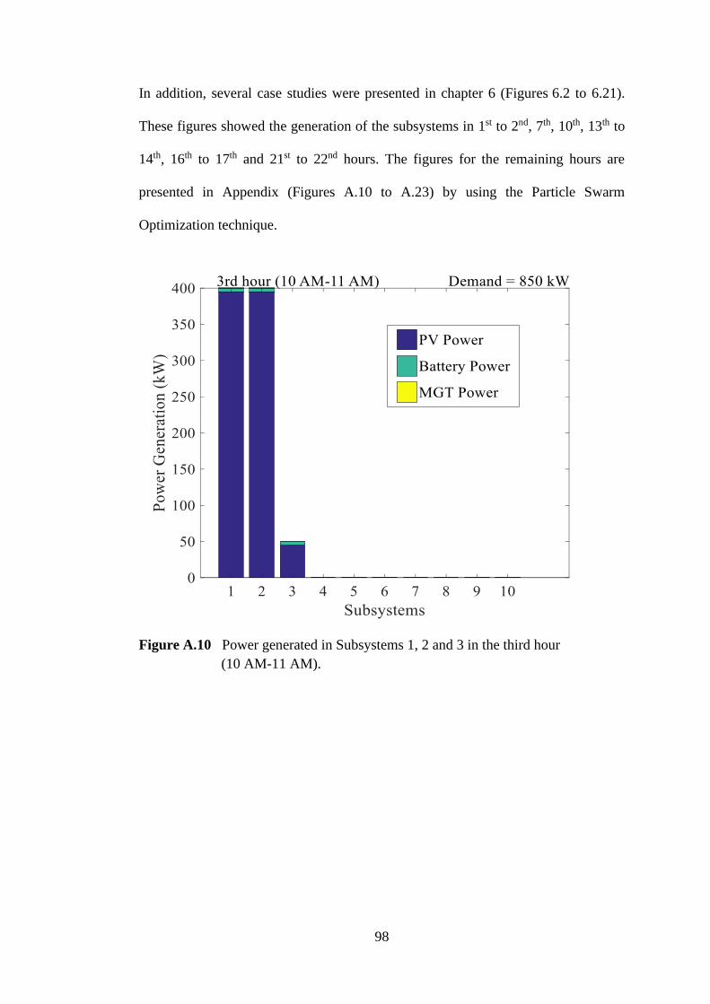
98
In addition, several case studies were presented in chapter 6 (Figures 6.2 to 6.21).
These figures showed the generation of the subsystems in 1st to 2nd, 7th, 10th, 13th to
14th, 16th to 17th and 21st to 22nd hours. The figures for the remaining hours are
presented in Appendix (Figures A.10 to A.23) by using the Particle Swarm
Optimization technique.
Figure A.10 Power generated in Subsystems 1, 2 and 3 in the third hour
(10 AM-11 AM).

99
Figure A.11 Power generated in Subsystems 1, 2, 4 and 6 in the fourth hour
(11 AM-12 PM).
Figure A.12 Power generated in Subsystems 1, 2, 3 and 5 in the fifth hour
(12 PM-1 PM).

100
Figure A.13 Power generated in Subsystems 1, 2, 3, 4 and 5 in the sixth hour
(1 PM-2 PM).
Figure A.14 Power generated in Subsystems 1, 2, 3, 4 and 5 in the eighth hour
(3 PM-4 PM).

101
Figure A.15 Power generated in Subsystems 1, 2, 3, 4, 5, 6 and 7 in the ninth hour
(4 PM-5 PM).
Figure A.16 Power generated in Subsystems 1, 2, 3, 4, 5, 6, 7 and 8 in the eleventh
hour (6 PM-7 PM).

102
Figure A.17 Power generated in Subsystems 1, 2, 3, 4, 5, 6, 7, 8 and 9 in the twelfth
hour (7 PM-8 PM).
Figure A.18 Power generated in Subsystems 1, 2, 3, 4 and 5 in the fifteenth hour
(10 PM-11 PM).

103
Figure A.19 Power generated in Subsystems 1, 2, 3, 4 and 5 in the eighteenth hour
(1 AM-2 AM).
Figure A.20 Power generated in Subsystems 1, 2, 3, 4 and 5 in the nineteenth hour
(2 AM-3 AM).

104
Figure A.21 Power generated in Subsystems 1, 2, 3, 4, 5, 6 and 7 in the twentieth
hour (3 AM-4 AM).
Figure A.22 Power generated in Subsystems 1, 2 and 5 in the twenty-third hour
(6 AM-7 AM).

105
Figure A.23 Power generated in Subsystems 1 and 2 in the twenty-fourth hour
(7 AM-8 AM).
Table A.1 lists the Dynamic Programming technique performance results for twenty-
four hours. Table A.2 lists the Particle Swarm Optimization technique performance
results for twenty-four hours as we did in the case of DP. These results were obtained
for solving only the Unit Commitment problems by using the DP and PSO techniques.
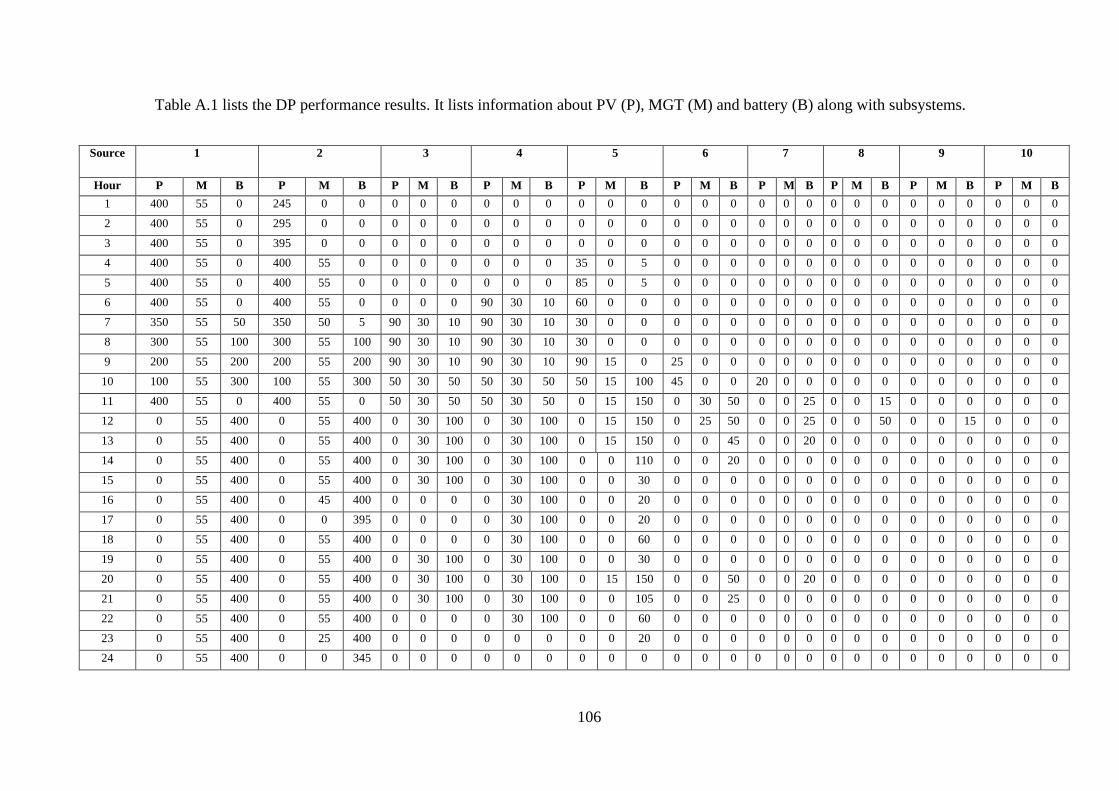
106
Table A.1 lists the DP performance results. It lists information about PV (P), MGT (M) and battery (B) along with subsystems.
Source
1 2 3 4 5 6 7 8 9 10
Hour P M B P M B P M B P M B P M B P M B P M B P M B P M B P M B
1 400 55 0 245 0 0 0 0 0 0 0 0 0 0 0 0 0 0 0 0 0 0 0 0 0 0 0 0 0 0
2 400 55 0 295 0 0 0 0 0 0 0 0 0 0 0 0 0 0 0 0 0 0 0 0 0 0 0 0 0 0
3 400 55 0 395 0 0 0 0 0 0 0 0 0 0 0 0 0 0 0 0 0 0 0 0 0 0 0 0 0 0
4 400 55 0 400 55 0 0 0 0 0 0 0 35 0 5 0 0 0 0 0 0 0 0 0 0 0 0 0 0 0
5 400 55 0 400 55 0 0 0 0 0 0 0 85 0 5 0 0 0 0 0 0 0 0 0 0 0 0 0 0 0
6 400 55 0 400 55 0 0 0 0 90 30 10 60 0 0 0 0 0 0 0 0 0 0 0 0 0 0 0 0 0
7 350 55 50 350 50 5 90 30 10 90 30 10 30 0 0 0 0 0 0 0 0 0 0 0 0 0 0 0 0 0
8 300 55 100 300 55 100 90 30 10 90 30 10 30 0 0 0 0 0 0 0 0 0 0 0 0 0 0 0 0 0
9 200 55 200 200 55 200 90 30 10 90 30 10 90 15 0 25 0 0 0 0 0 0 0 0 0 0 0 0 0 0
10 100 55 300 100 55 300 50 30 50 50 30 50 50 15 100 45 0 0 20 0 0 0 0 0 0 0 0 0 0 0
11 400 55 0 400 55 0 50 30 50 50 30 50 0 15 150 0 30 50 0 0 25 0 0 15 0 0 0 0 0 0
12 0 55 400 0 55 400 0 30 100 0 30 100 0 15 150 0 25 50 0 0 25 0 0 50 0 0 15 0 0 0
13 0 55 400 0 55 400 0 30 100 0 30 100 0 15 150 0 0 45 0 0 20 0 0 0 0 0 0 0 0 0
14 0 55 400 0 55 400 0 30 100 0 30 100 0 0 110 0 0 20 0 0 0 0 0 0 0 0 0 0 0 0
15 0 55 400 0 55 400 0 30 100 0 30 100 0 0 30 0 0 0 0 0 0 0 0 0 0 0 0 0 0 0
16 0 55 400 0 45 400 0 0 0 0 30 100 0 0 20 0 0 0 0 0 0 0 0 0 0 0 0 0 0 0
17 0 55 400 0 0 395 0 0 0 0 30 100 0 0 20 0 0 0 0 0 0 0 0 0 0 0 0 0 0 0
18 0 55 400 0 55 400 0 0 0 0 30 100 0 0 60 0 0 0 0 0 0 0 0 0 0 0 0 0 0 0
19 0 55 400 0 55 400 0 30 100 0 30 100 0 0 30 0 0 0 0 0 0 0 0 0 0 0 0 0 0 0
20 0 55 400 0 55 400 0 30 100 0 30 100 0 15 150 0 0 50 0 0 20 0 0 0 0 0 0 0 0 0
21 0 55 400 0 55 400 0 30 100 0 30 100 0 0 105 0 0 25 0 0 0 0 0 0 0 0 0 0 0 0
22 0 55 400 0 55 400 0 0 0 0 30 100 0 0 60 0 0 0 0 0 0 0 0 0 0 0 0 0 0 0
23 0 55 400 0 25 400 0 0 0 0 0 0 0 0 20 0 0 0 0 0 0 0 0 0 0 0 0 0 0 0
24 0 55 400 0 0 345 0 0 0 0 0 0 0 0 0 0 0 0 0 0 0 0 0 0 0 0 0 0 0 0

107
Table A.2 lists the PSO performance results. It lists information about PV (P), MGT (M) and battery (B) along with subsystems.
Source 1 2 3 4 5 6 7 8 9
10
Hour P M B P M B P M B P M B P M B P M B P M B P M B P M B P M B
1 395 0 5 295 0 5 0 0 0 0 0 0 0 0 0 0 0 0 0 0 0 0 0 0 0 0 0 0 0 0
2 395 0 5 345 0 5 0 0 0 0 0 0 0 0 0 0 0 0 0 0 0 0 0 0 0 0 0 0 0 0
3 395 0 5 395 0 5 45 0 5 0 0 0 0 0 0 0 0 0 0 0 0 0 0 0 0 0 0 0 0 0
4 395 0 5 395 0 5 0 0 0 100 0 0 0 0 0 50 0 0 0 0 0 0 0 0 0 0 0 0 0 0
5 400 0 0 400 0 0 50 0 0 0 0 0 150 0 0 0 0 0 0 0 0 0 0 0 0 0 0 0 0 0
6 395 0 5 395 0 5 90 0 5 90 0 5 90 0 5 0 0 0 0 0 0 0 0 0 0 0 0 0 0 0
7 395 55 5 395 5 5 100 0 0 100 0 0 90 0 0 0 0 0 0 0 0 0 0 0 0 0 0 0 0 0
8 395 55 5 395 55 5 100 0 0 100 0 0 90 0 0 0 0 0 0 0 0 0 0 0 0 0 0 0 0 0
9 370 55 30 370 55 30 80 0 20 80 0 20 100 0 0 50 0 0 10 0 0 0 0 0 0 0 0 0 0 0
10 200 55 200 200 55 200 30 30 70 30 30 70 50 0 100 50 0 0 30 0 0 0 0 0 0 0 0 0 0 0
11 150 55 250 150 55 250 30 30 70 30 30 70 40 0 110 20 0 30 20 0 30 30 0 0 0 0 0 0 0 0
12 100 55 300 100 55 300 10 30 90 10 30 90 40 0 110 20 0 30 20 0 30 20 0 30 0 0 30 0 0 0
13 0 55 400 0 55 400 0 30 100 0 30 100 0 0 150 0 0 50 0 0 30 0 0 0 0 0 0 0 0 0
14 0 55 400 0 55 400 0 0 100 0 0 100 0 0 150 0 0 40 0 0 0 0 0 0 0 0 0 0 0 0
15 0 55 400 0 55 400 0 0 100 0 0 100 0 0 90 0 0 0 0 0 0 0 0 0 0 0 0 0 0 0
16 0 0 400 0 0 400 0 0 100 0 0 100 0 0 50 0 0 0 0 0 0 0 0 0 0 0 0 0 0 0
17 0 0 400 0 0 400 0 0 50 0 0 100 0 0 50 0 0 0 0 0 0 0 0 0 0 0 0 0 0 0
18 0 0 400 0 0 400 0 0 100 0 0 100 0 0 100 0 0 0 0 0 0 0 0 0 0 0 0 0 0 0
19 0 55 400 0 55 400 0 0 100 0 0 100 0 0 90 0 0 0 0 0 0 0 0 0 0 0 0 0 0 0
20 0 55 400 0 55 400 0 30 100 0 30 100 0 0 150 0 0 50 0 0 30 0 0 0 0 0 0 0 0 0
21 0 55 400 0 55 400 0 0 100 0 0 100 0 0 150 0 0 40 0 0 0 0 0 0 0 0 0 0 0 0
22 0 0 400 0 0 400 0 0 100 0 0 100 0 0 100 0 0 0 0 0 0 0 0 0 0 0 0 0 0 0
23 0 0 400 0 0 400 0 0 0 0 0 0 0 0 100 0 0 0 0 0 0 0 0 0 0 0 0 0 0 0
24 0 0 400 0 0 400 0 0 0 0 0 0 0 0 0 0 0 0 0 0 0 0 0 0 0 0 0 0 0 0