waiting line management 7 - bangladesh open university · waiting line management ... because there...
TRANSCRIPT
Waiting Line
Management
Unit Introduction
The phenomena of waiting are common in business and industry. In most
business situations, the customers are the machines, not people, like trucks
waiting to be unloaded, ships waiting to dock, orders waiting to be filled, jobs
waiting to be processed. Waiting is annoying, but we do wait. Given time most of
the facilities can process more than they are called upon to process. The waiting
line theory or queue theory is commonly used in planning and analyzing service
capacity of a system. Based on type of the structure a specific queue model, from
innumerous models, is applied. The main characteristics under consideration are,
the arrival pattern of customers, queue discipline, length of the queue, queue
behavior etc. Because there are large number of possible models, a notation set
has been developed by D.G. Kendall that makes it easy to identify the model
applicable for a particular system. After finding out the values of different
measures of performance, the next is to determine the efficiency of the service
system. At the very beginning it should be remembered that all the measures of
performances are not required to determine the efficiency of the system.
Therefore this unit will include a discussion on introduction of the concept of
waiting line management, characteristics of waiting line, and the methodologies
of waiting line management.
7
School of Business
Unit- 7 Page- 166
Bangladesh Open University
Production Operations Management Page- 167
Lesson One: Introduction To Waiting Line Management
Lesson Objectives
After completing this lesson you will be able to:
� Explain the theories of satisfaction
� Discuss the quality factors affecting satisfaction
� Justify the customer’s reaction to delay
� Describe the methods of delay management
Many things in life are worth waiting for. We would not mind waiting for the
course completion to earn an MBA. We love to wait for good news from our dear
ones. Waiting in line is common in our day to day life. We wait in line to avail
buses, to deposit our money in the bank, to pay bills, to buy goods or to use lift.
The phenomena of waiting are also common in business and industry. We find
mechanics waiting for their tool cribs or standing idle for mechanics. Students
wait for photocopy of books. In most business situations, the customers are the
machines, not people, like trucks waiting to be unloaded, ships waiting to dock,
orders waiting to be filled, jobs waiting to be processed.
Waiting is annoying, but we do wait. It is estimated that we spend at least 10% of
our working moments waiting. Given time most of the facilities can process more
than they are called upon to process. But still, because of the random nature of
arrival of customers, waiting is bound to occur. The waiting line theory or queue
theory is commonly used in planning and analyzing service capacity of a system.
It is a mathematical approach not only to analyze waiting times, but also used in
large number of situations for example,
• to determine the number of beds in a hospital or required size of a
restaurant
• to determine the number of runways in an airport
• to determine the number of lifts in a building or the number of ATM
machines in a bank branch
• to determine the number of switches in a telephone box
• to schedule delivery of jobs.
Delay in service has a direct bearing on customer’s satisfaction. To reduce
delays, management needs to expand capacity. But it is expensive to increase
capacity. Managers have to weigh the cost of providing additional capacity
against potential decrease in delays in service. Therefore, management is
interested in finding the appropriate level of service that will ensure the customer
satisfaction.
Theories on Customer Satisfaction During and after consumption of goods and services, consumers develop a feeling about
the quality of the commodity. The feeling may be positive or negative. If the consumer
develops a positive feeling, we say that the consumer is satisfied with the service or
product. If the consumer develops a negative feeling we say that the consumer is
dissatisfied. Consumer satisfaction or dissatisfaction is a post-acquisition and post
consumption judgement of the quality of service or product. Consumer satisfaction
has been defined as “the overall attitude consumers have towards a good or
service after they have acquired or used it”1.
1 Robert A Westbrook and Richard L. Oliver, The Dimensionality of consumption Emotion Patterns and
Consumer Satisfaction, Journal of Consumer Research, Vol 18 (June 1991).
The waiting line theory
is a mathematical
approach not only to
analyze waiting times,
but also used in large
number of situations
Consumer satisfaction or
dissatisfaction is a post-
acquisition and post
consumption judgement
of the quality of service
or product.
School of Business
Unit- 7 Page- 168
From a managerial perspective, maintaining and enhancing customer satisfaction
is critical. Satisfied customers are important to companies because, on average,
approximately 70% of all sales are derived from repeated purchases. Firms can
no longer maintain volume or profits by seeking new customers. Attracting new
customers are expensive. It is much cheaper to keep the current customers happy
and satisfied. After the purchase and consumption of products or services,
customers compare their pre-purchase perception of the quality of the
product/service and their post-consumption perception of the quality of the
service/product. Depending how the actual performance measures against
expected performance, the customer will experience positive, negative or neutral
emotions. To understand how consumers develop satisfaction or dissatisfaction
regarding a service or a product, we will look into
1. Confirmation model
2. Disconfirmation model, and
3. Equity theory of satisfaction
1. The confirmation model: Early thinkers about consumer satisfaction
assumed it as meeting expectation of consumers. The confirmation model
describes the successful outcome as contentment. We are content when our
computer is working without problem or the photocopy machine does not get
jammed. This low arousal state is matched by discontent when negative
expectations are met. But poor satisfactions are ignored because of habit.
People put up with many troubles because they are used to them and no
longer notice them as a problem. For example, we are used to slow responses
of the salesmen, late arrival of buses, or congestion in roads. The tolerance of
deficiencies in services or products is explained by the “adaptation theory”.
This theory makes expectation relative to experience. As long as gap
between expectation and reality is small, the customers tend to be
accommodative. Only when the gap is too large and does affect the
adaptability of the customers it leads to discontentment.
2. The disconfirmation model: Unlike the Confirmation Model, the
Disconfirmation Model focuses on high arousal conditions. The model
attempts to explain satisfaction or dissatisfaction of consumers by explaining
the gap between expectation and reality. If the product or service has more
features than expected, the customer is surprised and is satisfied. On the
other hand, if the product or service contains fewer features than expected,
again the customer is surprised and is dissatisfied. The model recognizes that
people use standards of assessment to judge a product or service. According
to this model satisfaction is a cognitive state of a consumer of being
adequately or inadequately rewarded for the sacrifices he/she has made to
acquire and consume the service or product. In the disconfirmation model,
the degree of satisfaction or dissatisfaction depends on,
(i) the size of discrepancy between expectation and experience,
(ii) value of the product, and
(iii) the perception of consumer regarding the performance of the
service or product.
The larger the discrepancy between expectation and experience the more
aroused (positive or negative) we get. The more money we spend for a
service or product the higher the expectation. Finally, the higher the
expectation and the higher the resulting experience the higher is the
satisfaction.
Disconfirmation model
explain satisfaction or
dissatisfaction of
consumers by explaining
the gap between
expectation and reality.
Bangladesh Open University
Production Operations Management Page- 169
3. The equity theory: Another approach to explain consumer satisfaction is the
Equity Theory. The Equity Theory holds that the customer will analyze the
outcome of the transaction by comparing the value of the input he has put in
the effort and the value of input provided by the other party. If the consumer
feels that his input contribution is more than that of the other party he will
develop a feeling of inequity. According to this theory, the norm is that each
party to the exchange should be treated equitably. The ratios of outcomes and
inputs of both the parties should be equal. Equity theory holds that
satisfaction results from comparing one’s outcomes and inputs with that of
others. From the consumers perspective inputs are information, money, effort
and time spent to acquire the good or service. Outcome consists of receiving
the goods or services, performance of the product, and the feeling associated
with the use of the product or service.
Factors Affecting Customer Satisfaction
Consumer’s expectation of a product or service is derived from the perceived
quality of the commodity. Quality has multiple dimensions in the mind of the
customer, and applying them one or more at a time at any one time. Quality is
defined as customer’s overall evaluation of the excellence of the performance of
a good or service. Because of the difference between a product and a service,
they have different quality dimensions. Table 7.2.1 provides a summary of the
quality dimensions of products and services. They are discussed in detail below:
Table 7.2.1: Dimensions of quality
Dimensions Description
Quality of Products
Confirmation to
Specification
Degree to which the product meets industrial
standards
Fitness of Use Chances of failure or malfunction
Value Worth of the product in relation to similar products
After Sales Services Ease of repair, and timeliness of personnel
Psychological
Impression
The look, feel and sound of the product
Quality of Services
Tangibles Physical facilities, appearance and equipment
Reliability Dependability of employees
Responsiveness Prompt response
Assurance Ability and knowledge of employees
Empathy Individualized attention
Customer’s Response to Delay
Customers do not like to wait for services. But delay in delivery of service is a
perennial feature of service outlets. Customers have to wait to deposit or
withdraw money from bank; they have to join queues to post their letters; they
Equity theory analyze
the outcome of the
transaction by
comparing the value of
the input in effort and
the value of input
provided by other party.
Activity: Choose a service product of your choice and think why
you as a customer need better service for that product? Exchange
your views with any of your friend(s).
From the economic point of view waiting is wasteful nor is it productive.
School of Business
Unit- 7 Page- 170
have to wait to buy tickets for bus; they also have to wait for transport and get
held up in traffic jams. For the individuals it is frustrating to wait. For the
economy it is wasteful because people waiting for service is neither consuming
nor they are producing. But the service providers are unable to remove delays in
their system. Even if they plan for peak demand they still end up with queues in
their system. Waiting for service is a result of the random arrival of the
customers. Customers arrive for service at random, creating localized peaks and
valleys in demand pattern. In most service outlets arrival of customers cannot be
programmed or scheduled. Researches show that, on average, people wait for
more than half an hour each day for different services and appointments.
a) Evaluation of service: Organizations that create delay by poor design of
their service facilities do so at their own peril. The customers consider
waiting a punishment, and they associate it with the whole service
experience. The longer the delay the lower is the evaluation of the whole
system. Many of our local organizations, specially the nationalized
institutions like banks, do not notice the irritations caused by delay.
b) Difference in Perception: There is a perpetual difference in opinion regarding the length of delays between the provider of service and the
customer. Customers always perceive to have waited long where as on the
other side the employees feel that the customers did not have to wait long.
Research found that when a customer at a bank thought the average delay
was 5.6 minutes the staff perception was 3.2 minutes and the actual delay
was 4.7 minutes.
c) Type of Dissatisfaction associated with delay: There are two types of
dissatisfaction associated with delay. A low involvement discontents when
delay is predicted and a high involvement affects when delay is not
predictable. As delays become more common and impose a more frequent
time-cost, people find it easier to put up with it.
d) Reasons for delay: If people are informed in advance as to the reason for
delay, they are less irritated and are patient in their waiting. The provision
of delay information is now standard among the transport operator, such as
airlines. Such information seems to be much appreciated despite the fact
that it does nothing to reduce waiting time.
e) Entertainment during Delay: People are less dissatisfied by delays if they can fill in their waiting time. For example, ANZ Grindlays Bank at their
Dhanmondi branch provides TV entertainment to their customers waiting
in queue; another is the provision of mirror in places where people have to
wait, e.g., at lifts in buildings. Additional examples are places where
waiting is very frequent, to provide the latest newspapers and magazines
for the customers to read. Research has shown that many of those waiting
do not even realize that they had been held up.
f) Control on delay: People become more irritated when they believe that the
service provider has control over the situation. If delays are beyond the
control of the providers, the customers are more tolerant to delays. For
example, airplane delayed due to inclemental weather does not create
negative impression about the provider. But on the other hand if the
customer believe that the delay is a result of slow check-in at the counter it
is bound to create negative feeling about the provider.
Customers perceive to
waited long to get service
where as employees feel
that customers did not
wait long.
Bangladesh Open University
Production Operations Management Page- 171
g) Delay at the beginning or end of the process: When delay occurs at the
beginning or at the end of the process it is evaluated more negatively than
when it occurs at the mid-process. It is better to impose delays in the
middle of the process, rather than at the end or beginning. In a restaurant it
is more appropriate to impose delay in providing food, but not to keep the
customers waiting before taking orders.
h) Value of exchange: People expect that their cost of waiting to be
compensated by appropriate rewards. This implies that those receiving
benefits in an exchange would be more tolerant to delays than those
incurring costs. For this reason, in a bank, those are in queue to pay bills
complain more than those waiting to encash their cheques.
Delay Management
Among the many quality dimensions that contribute to satisfaction or
dissatisfaction of customers, delay is one of the major and immediate
contributors to dissatisfaction. This is amply clear from the discussion in the
previous section. Management of service organizations should attempt to reduce
delay in providing services. There are three approaches that managers can adopt
to reduce delays:
1. Operations management
2. Influencing demand
3. Perception management
1. Operations management: Wherever feasible, management should try to
avoid delays by increasing service supply. This they can do by increasing
number of counter at peak hour and reduce it at off peak hours. Or they can
use experienced and quick workers during peak hours. This is easy to say but
very difficult to maintain. It is very expensive to provide additional facilities.
To plan for peak demand situation will result in under utilization at non-peak
hours. Because of the random nature of customer arrival, even if
management decides to provide for peak demand, they still will face delays
in their services. Some make use of part-time workers, others train their non-
service workers to assist the service workers during peak periods, and still
others use fast automatic machines.
2. Influencing demand: The second approach is to regulate demand or
influence demand to occur at specific time. Scheduling appointments, as
done by doctors for non-emergency patients, is one good example of
regulating demand for service. Providing incentive is another method of
regulating demand. For example, using differential price to shift demand to
particular period, e.g., Mondays are cheap days at the cinema in Britain.
Some even segment their customers according to the nature of service
required. If a group of customers need something that can be done very
quickly, they are given special line so they do not have to wait for the slower
customers. For example, at some departmental stores the customers with less
than five items have a fast channel to check out, whereas, customers with
more than five items have to pass through a slow line.
3. Perception management: The third approach is to try to ensure that the customers see the delay in a favorable way. By supplying delay information
customers can be made more tolerant to delays. By providing diversions can
the customers be made less dissatisfied to delays, like providing
Management of service
organizations should
attempt to reduce delay in
providing services.
Queuing ticket system
allows the customer to
conduct other business
while waiting.
Providing incentive is
another method of
regulating demand.
School of Business
Unit- 7 Page- 172
entertainment as they wait for service. Another way is the queuing ticket
system that allows the customer to conduct other business while waiting. For
example, in banks, the customers can sit down and read instead of standing in
line. But this approach implies that delay is normal and management is only
interested in alleviating the discomfort of waiting, not in eliminating it.
Employees that are not part of service should be kept out of sight. Nothing is
more frustrating to someone waiting in line to see employees, who potentially
could be serving those in line, doing nothing or working on other activities.
Greeting the customers by name, or providing some other special attention, can
go a long way toward overcoming the negative feeling of a long wait.
Psychologists suggest that the workers should invoke friendly actions such as
smiling when greeting or serving. Test result shows significant increase in
perceived friendliness of the servers in the eyes of the customers when the
servers smile while dealing with customers.
Activity: Think you as a bank manager in Bangladesh. Now why and
how you will manage your customers when you find that due to some
unavoidable circumstances they are waiting long for a service. Justify
your answer.
Bangladesh Open University
Production Operations Management Page- 173
Discussion questions
1. Describe the different theories of consumer satisfaction.
2. Describe the factors that influence consumers’ satisfaction?
3. How do consumers respond to delay?
4. What should management do to manage delays?
School of Business
Unit- 7 Page- 174
Lesson Two: Waiting Line Queuing System
Lesson Objectives
After completing this lesson you will be able to:
� Describe the major characteristics of waiting line
� Explain the arrival pattern
� Discuss the service pattern
Characteristics of the Queuing system
Analysis of waiting line problem starts with a description of the structure of the
service system. Based on type of the structure a specific queue model, of
innumerous models, is applied. The main characteristics under consideration are:
a) The calling population or population source
b) The arrival pattern of customers
c) The distribution of customer arrival
d) The service pattern or number of servers
e) The service time distribution
f) The queue discipline
g) The length of the queue
h) The queue behavior
i) The exit of customer from the system
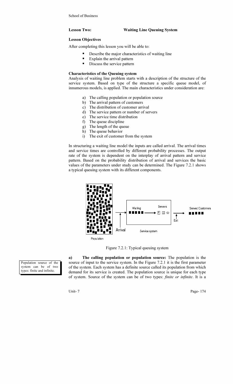
In structuring a waiting line model the inputs are called arrival. The arrival times
and service times are controlled by different probability processes. The output
rate of the system is dependent on the interplay of arrival pattern and service
pattern. Based on the probability distribution of arrival and services the basic
values of the parameters under study can be determined. The Figure 7.2.1 shows
a typical queuing system with its different components.
Figure 7.2.1: Typical queuing system
a) The calling population or population source: The population is the
source of input to the service system. In the Figure 7.2.1 it is the first parameter
of the system. Each system has a definite source called its population from which
demand for its service is created. The population source is unique for each type
of system. Source of the system can be of two types: finite or infinite. It is a
Population source of the
system can be of two
types: finite and infinite.
Bangladesh Open University
Production Operations Management Page- 175
major concern for the analyst to determine whether the source for potential
customer is finite or infinite. A finite population source refers to the limited size
customer pool that will use the service. If the source is finite, and a customer
leaves the population and joins the system for service, the population gets
reduced which, in turn, reduces the probability of creation of next demand for
service. For example, a photocopy machine in an office has a finite population
source. Demand for its use can arise from among that office employees, no one
outside the office can use the machine. So if an employee uses the machine, the
chance of another using it is very small. If the population source is too small it
may even affect the probability of an arrival.
Alternatively, an infinite population is one in which the number of customers in
the system doesn't affect the rate at which the population generates new arrivals.
For example, the photocopy machines at Nilket, New Market at Dhaka have an
infinite population source. Its customers are all living in and around Nilket area.
Because the customer population is large and only a small fraction is at any one
time demanding its service, the number of new arrivals it generates is not
affected by the number who is using or has already used its service. Such
population is called infinite population.
b) The arrival pattern of customers: Arrival pattern is also an important
issue to the analysts. The arrival into a service system can be scheduled or
unscheduled. When customers arrive at service centers by appointment it is
called scheduled arrival. For example, general patients can consult specialist
doctors only by appointment. Unscheduled arrivals are common in many service
centers like retail outlets or restaurants. Unscheduled arrivals are random in
nature and are also called random arrivals. Random arrivals are more common
than scheduled arrivals.
Arrivals can also be controlled or uncontrolled. The arrivals at a system are more
controlled than is generally recognized. Barbers may decrease their Friday
arrivals by charging more than other weekdays, or a doctor, in a private clinic,
not seeing more than a fixed number of patients a day. The simplest of all arrival-
control devices is having fixed business hours. But some service demands are
clearly uncontrollable, like hospital emergencies. Controlled arrivals are more
common than uncontrolled.
Arrivals can also be single or in batches. Customers can arrive in batches, such as
the arrival of family to a restaurant or garment factories receive orders for a
particular item in batches. When customers arrive individually or singly it is
called single arrival. For example, a housewife going for shopping at 1-Stop
Mall; a student going for class; or a person waiting to use the lift in a building.
c) The distribution of customer arrival: The arrival of customers for
services can be described as either average arrival rate or as average inter-
arrival time. Average arrival rate means the average number of arrivals per a
given time and average inter-arrival time means the average time between
arrivals, that is, the time between one arrival and the next. In case of scheduled
arrivals, the arrival rate is relatively predetermined, while that in unscheduled it
is a random variable and therefore we have to find its average time and also need
to find out its frequency distribution.
An infinite population is
one in which the
probability of future
arrival is not affected by
the number of customer
already in avenue.
Arrival pattern of customer can be classified as scheduled and unscheduled, or controlled and uncontrolled or even single and in batches.
Arrival of customers for
services can be described
by either average arrival
rate or by the average
inter-arrival time.
School of Business
Unit- 7 Page- 176
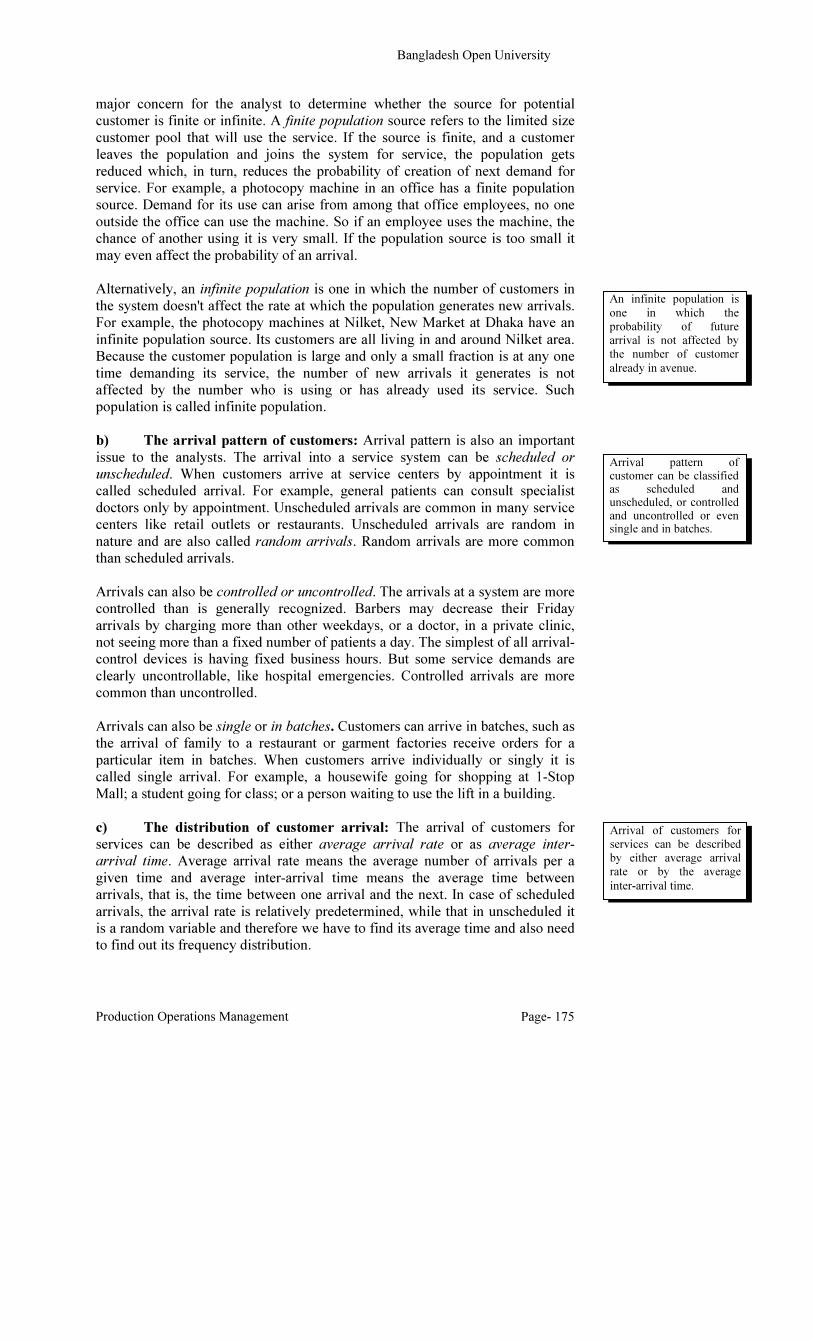
In scheduled arrival the arrival distribution is generally constant with exactly the
same time period between successive arrivals, as shown in the Figure: 7.2.1. It
would have same inter-arrival time (t) and with variance zero (0). But in case of
random arrivals, the time between arrivals would vary and would have a positive
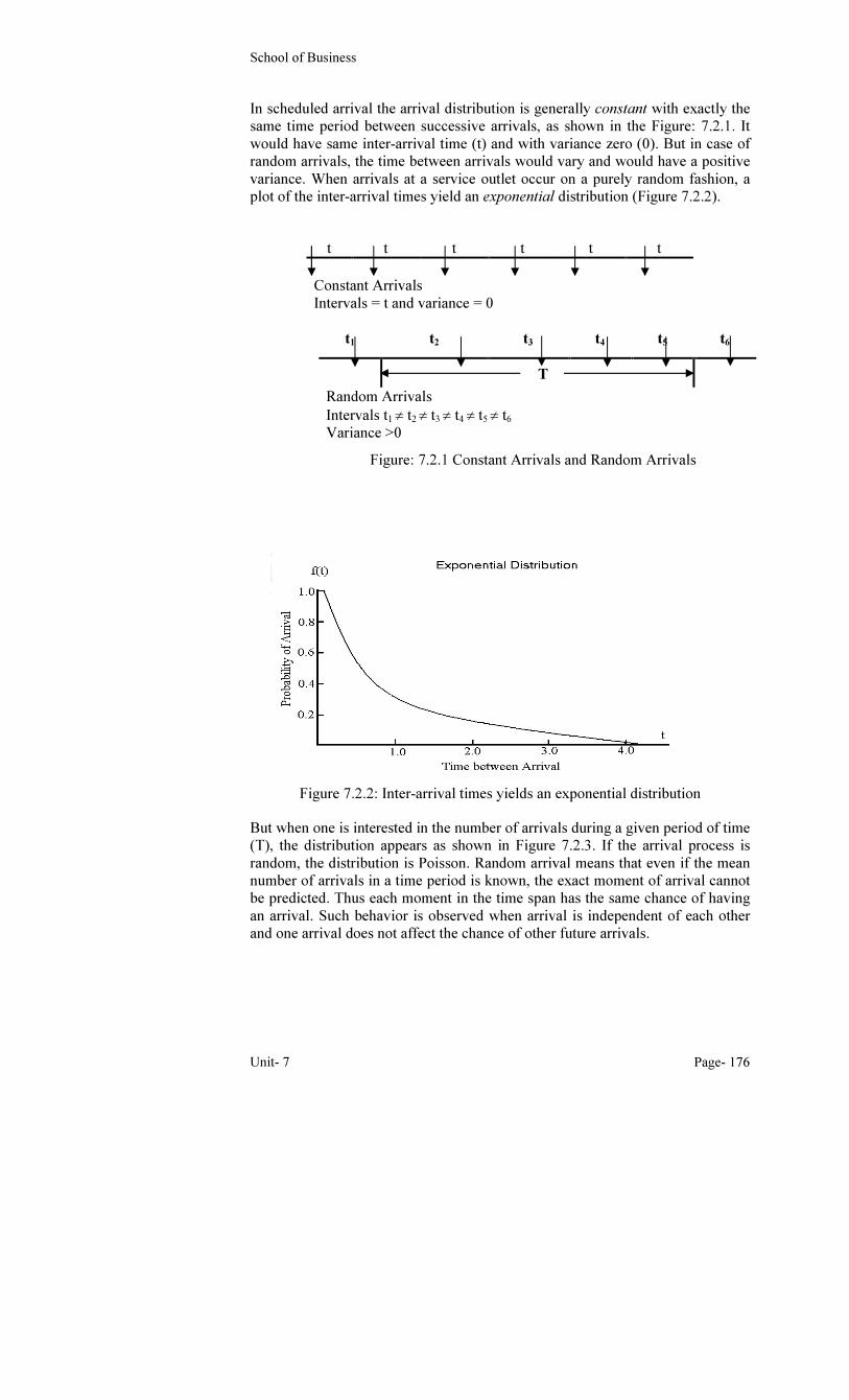
variance. When arrivals at a service outlet occur on a purely random fashion, a
plot of the inter-arrival times yield an exponential distribution (Figure 7.2.2).
t t t t t t
Constant Arrivals
Intervals = t and variance = 0
t1 t2 t3 t4 t5 t6
T
Random Arrivals
Intervals t1 ≠ t2 ≠ t3 ≠ t4 ≠ t5 ≠ t6
Variance >0
Figure 7.2.2: Inter-arrival times yields an exponential distribution
But when one is interested in the number of arrivals during a given period of time
(T), the distribution appears as shown in Figure 7.2.3. If the arrival process is
random, the distribution is Poisson. Random arrival means that even if the mean
number of arrivals in a time period is known, the exact moment of arrival cannot
be predicted. Thus each moment in the time span has the same chance of having
an arrival. Such behavior is observed when arrival is independent of each other
and one arrival does not affect the chance of other future arrivals.
Figure: 7.2.1 Constant Arrivals and Random Arrivals

Bangladesh Open University
Production Operations Management Page- 177
Figure 7.2.3: Interested number of arrivals in a given period
Poisson distribution is commonly observed in average arrival rate and
exponential distribution for inter-arrival time. Other distributions observed in
queuing situation are hyperexponential, hyperpoisson, and erlang distribution
with k parameter. The average arrival rate is usually designated by the Greek
letter lambda, λ and interarrival time, which is reciprocal of average rate, is 1/λ.
d) The service pattern or number of servers: The capacity of a service
system is a function of the capacity of each server and the number of servers
being used. The terms server and channel are synonymous, and it is generally
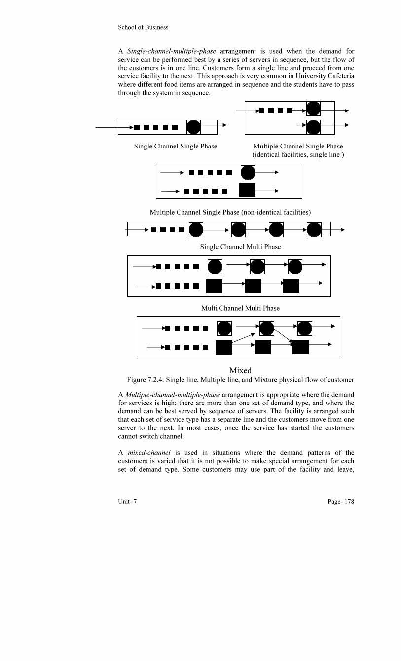
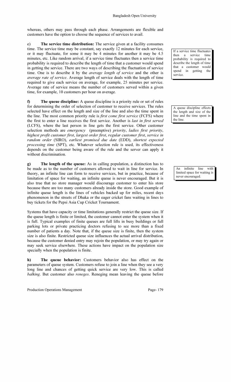
assumed that each channel can handle one customer at a time. The physical flow
of customers through the facility can be in single line or in multiple line, or
mixture of both. The format of flow depends on the nature of service demanded
and the pattern of service offered.
A Single-channel-single-phase flow is the simplest of all waiting line formats.
When all the services demanded by the customer can be performed by a single
server the facility is arranged such that customers form a single line and go
through the service facility one at a time. Examples are checkout counter at retail
stores and machine that must process several batches of parts.
A Multiple-channel-single-phase (identical service) approach is used where the
demand for services are identical but is very high to warrant use of more than one
server for the same type of service. Depending on the design of the system,
customers may form separate lines in front of each server or they may form a
single line but separate into different lines at the point of service. This approach
is also known as snake-line queue. It is commonly seen in service centers with
high service demand but low in waiting space, like Standard Chartered Grindlays
Bank office at Dhanmondi, Dhaka.
A Multiple-channel-single-phase (non-identical service) is a format used when
different set of customers has different type of service requirement. Service
desired by customers are not identical. Each demand set is passed through the
system in separate lines, but for each line a single server performs the desired
services. For example, we observe in bank separate counters for deposits and
encashment of cheques.
The physical flow of
customers through the
facility can be in single
line or in multiple line, or
mixture of both.
School of Business
Unit- 7 Page- 178
A Single-channel-multiple-phase arrangement is used when the demand for
service can be performed best by a series of servers in sequence, but the flow of
the customers is in one line. Customers form a single line and proceed from one
service facility to the next. This approach is very common in University Cafeteria
where different food items are arranged in sequence and the students have to pass
through the system in sequence.
Single Channel Single Phase
Multiple Channel Single Phase
(identical facilities, single line )
Multiple Channel Single Phase (non-identical facilities)
Single Channel Multi Phase
Multi Channel Multi Phase
Mixed
Figure 7.2.4: Single line, Multiple line, and Mixture physical flow of customer
A Multiple-channel-multiple-phase arrangement is appropriate where the demand
for services is high; there are more than one set of demand type, and where the
demand can be best served by sequence of servers. The facility is arranged such
that each set of service type has a separate line and the customers move from one
server to the next. In most cases, once the service has started the customers
cannot switch channel.
A mixed-channel is used in situations where the demand patterns of the
customers is varied that it is not possible to make special arrangement for each
set of demand type. Some customers may use part of the facility and leave,
Bangladesh Open University
Production Operations Management Page- 179
whereas, others may pass through each phase. Arrangements are flexible and
customers have the option to choose the sequence of services to avail.
e) The service time distribution: The service given at a facility consumes
time. The service time may be constant, say exactly 12 minutes for each service,
or it may fluctuate, for some it may be 4 minutes for another it may be 4.5
minutes, etc. Like random arrival, if a service time fluctuates then a service time
probability is required to describe the length of time that a customer would spend
in getting the service. There are two ways of describing the fluctuation of service
time. One is to describe it by the average length of service and the other is
average rate of service. Average length of service deals with the length of time
required to give each service on average, for example, 25 minutes per service.
Average rate of service means the number of customers served within a given
time, for example, 10 customers per hour on average.
f) The queue discipline: A queue discipline is a priority rule or set of rules
for determining the order of selection of customer to receive services. The rules
selected have effect on the length and size of the line and also the time spent in
the line. The most common priority rule is first come first service (FCFS) where
the first to enter a line receives the first service. Another is last in first served
(LCFS), where the last person in line gets the first service. Other customer
selection methods are emergency (preemptive) priority, ladies first priority,
highest profit customer first, largest order first, regular customer first, service in
random order (SIRO), earliest promised due date (EDD), shortest expected
processing time (SPT), etc. Whatever selection rule is used, its effectiveness
depends on the customer being aware of the rule and the server can apply it
without discrimination.
g) The length of the queue: As in calling population, a distinction has to
be made as to the number of customers allowed to wait in line for service. In
theory, an infinite line can form to receive services, but in practice, because of
limitation of space for waiting, an infinite queue is never encouraged. But it is
also true that no store manager would discourage customer to enter his store
because there are too many customers already inside the store. Good example of
infinite queue length is the lines of vehicles backed up for miles, recent days
phenomenon in the streets of Dhaka or the eager cricket fans waiting in lines to
buy tickets for the Pepsi Asia Cup Cricket Tournament.
Systems that have capacity or time limitations generally restrict the queue size. If
the queue length is finite or limited, the customer cannot enter the system when it
is full. Typical examples of finite queues are full lifts in busy buildings or full
parking lots or private practicing doctors refusing to see more than a fixed
number of patients a day. Note that, if the queue size is finite, then the system
size is also finite. Restricted queue size influences the actual arrival distribution,
because the customer denied entry may rejoin the population, or may try again or
may seek service elsewhere. These actions have impact on the population size
specially when the population is finite.
h) The queue behavior: Customers behavior also has effect on the
parameters of queue system. Customers refuse to join a line when they see a very
long line and chances of getting quick service are very low. This is called
balking. But customer also reneges. Reneging mean leaving the queue before
If a service time fluctuates
then a service time
probability is required to
describe the length of time
that a customer would
spend in getting the
service.
A queue discipline effects
the length and size of the
line and the time spent in
the line.
An infinite line with
limited space for waiting is
never encouraged.
School of Business
Unit- 7 Page- 180
getting served. Customers waiting in line are either impatient or patient. Those
who renege or bulk are called impatient customers. Patient customers are those
who enter the system and do not leave till served. But patient customer, while
waiting for service, seeing a shorter line may switch between lines. This is called
jockeying. Customers also recycle by returning to the queue immediately after
obtaining service. This phenomenon is commonly observed when the authority
restricts the number of tickets that an individual can buy as in Pepsi Asia Cup
Tournament.
i) The exit of customer from the system: Once the customer is served,
two exit fates are possible: (a) the customer may return to the population source
and immediately become candidate for re-arrival, or (b) the customer exits the
system but does not return to the calling population. The first case can be
illustrated by the customer who patronage the same restaurant for every meal or
the machine in a factory that has been repaired and has joined production line. In
the second case, the served customer has a zero probability of returning for re-
service. For example, a patient who had an appendectomy operation will never
require a second similar operation. If the population is finite the non-return of
served customer to the population will modify the population structure and will
also modify the arrival rate for service.
Customers refuse to join a
line when they see a very
long line and chances of
getting quick service are
very low.
Bangladesh Open University
Production Operations Management Page- 181
Discussion questions
1. Explain how the source population can affect arrival rate.
2. What do you mean by arrival pattern?
3. Describe the common service system structure in use.
4. What do you mean by single-channel-multi-phase queue?
5. Describe, in brief, the different components of a service system.
School of Business
Unit- 7 Page- 182
Lesson Three: Waiting Line Methodology (i)
Lesson Objectives
After completing this lesson you will be able to:
� Explain the managerial problems in waiting line situation
� Describe the methodology of queue analysis
The Managerial Problems in Waiting Line
The central problem in every waiting line situation is a trade-off decision. There
are two basic categories of cost in queuing situation. The first is the cost of
providing service. The greater the service level, the higher the cost of providing
service. The second cost is related to customer waiting. Waiting cost decreases as
the capacity to provide service increases.
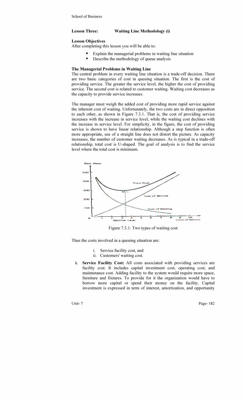
The manager must weigh the added cost of providing more rapid service against
the inherent cost of waiting. Unfortunately, the two costs are in direct opposition
to each other, as shown in Figure 7.3.1. That is, the cost of providing service
increases with the increase in service level, while the waiting cost declines with
the increase in service level. For simplicity, in the figure, the cost of providing
service is shown to have linear relationship. Although a step function is often
more appropriate, use of a straight line does not distort the picture. As capacity
increases, the number of customer waiting decreases. As is typical in a trade-off
relationship, total cost is U-shaped. The goal of analysis is to find the service
level where the total cost is minimum.
Figure 7.3.1: Two types of waiting cost
Thus the costs involved in a queuing situation are:
i. Service facility cost, and
ii. Customers' waiting cost.
i. Service Facility Cost: All costs associated with providing services are
facility cost. It includes capital investment cost, operating cost, and
maintenance cost. Adding facility to the system would require more space,
furniture and fixtures. To provide for it the organization would have to
borrow more capital or spend their money on the facility. Capital
investment is expressed in term of interest, amortization, and opportunity
Bangladesh Open University
Production Operations Management Page- 183
costs. Thus, cost of capital increases with the increase in facility or service
level. Operating cost includes cost of labor, energy, and materials required
for the additional facility. Additional facility would require additional
maintenance, repair, insurance, taxes, rental of space, and other fixed costs.
ii. Waiting Cost of Customers: Customers waiting for service also incur
cost. A customer who is waiting is not producing. The longer they wait the
longer the time they waste in non-productive activity. In some cases, it is
easy to assess the cost of waiting. When the customer belongs to the same
organization as those providing services, the cost of waiting is the wage
wasted while waiting. For example, if a worker has to wait in line to use a
computer, his waiting cost is the wage for the period he has to wait for the
computer.
In other situations, the cost of waiting cannot be determined so easily. For
example, if the customer were external to the organization providing service,
then what would be the cost of waiting? When the same organization have
different levels of customers how do we assess their lost wages? Other questions
that arise are, is the cost directly proportional to the waiting time? What is the
cost of ill will resulting from long waiting? What is the cost of lost sales, when
customers get impatient and leave? etc. Answers to such questions are not
simple, because they raise questions on personal values, social priorities, and
other qualitative factors.
Therefore, the total cost (TC) of a queue system are equal to the sum of cost of
providing service (CF) and the cost of waiting (CW). That is,
TC = CF + CW
Where,
TC = Total cost of the system
CF = Cost of providing service
CW = Customers' cost of waiting for service
The cost of waiting (CW) per unit time for the queuing system as a whole is given
by:
CW = WλC = LC
Where,
CW = Total cost of waiting
W = Average time waiting in the system
λ = Customer rate of arrival
C = Waiting cost per customer
L = Average number of customer in the system
The management may have the objective of minimizing total cost of services
(both facility and waiting cost) or achieving a specific level of services or both.
Longer the people wait the
longer the time they waste
in non-productive activity.
Activity: As a manager of a nationalized bank branch, how would you
identify the cost of waiting of your customers? Justify.
School of Business
Unit- 7 Page- 184
i. Cost minimization: Where both the facility cost and waiting cost can be
assessed easily, management would try to provide a service level that
would minimize total cost of the system.
ii. Specific service level: As a policy matter management may try to
achieve a specific level of service, disregarding the cost of service. For
example, a fast food restaurant advertise that customer does not have to
wait for more than three minutes for a burger, or a private mobile
telephone company promise to provide new connection within 24 hours,
or a service facility should be in use at least 75 percent of the time.
Determining the best level of service is a matter of organization policy
and is influenced by external factors as competition and consumer
pressures, etc.
Methodology of queuing analysis
Queuing can be analyzed by either mathematical process or by simulation. Here
we will describe the mathematical procedure. The method is basically a
descriptive tool of analysis. Unlike most other mathematical procedure it does
not provide any optimum solution rather it only describes the parameter of the
queue system. The major objective of this method is to predict the behavior of
the system to reflect its operating characteristics or measures of performance.
Management needs this set of information to determine the appropriate service
level of the system. Although queuing theory is basically descriptive, it can be
used to determine the optimum number of servers or optimum speed of service,
but such applications are very limited. The entire process of analyzing a queuing
system involves the following three steps:
1. Establish the performance criteria to measure.
2. Compute the measures of performance.
3. Analyze the situation and take action, if required.
1. Establish the performance criteria to measure: An operations manager’s
main aim is to improve the efficiency of the system and also balance the cost
involved. Typically the operations manager looks at the following measures
to evaluate the existing or proposed service system:
i. Queue Length: The queue length or the number of customer in the
line reflects one of two conditions. Short line means either a very
good customer service or it means the system has too much service
capacity. Similarly, a long queue may indicate poor service or the
need to increase capacity. For these reasons, the first parameter that
any operations manager looks for is the line size.
ii. Number of customers in the system: There is a major difference
between number of customer in line and number of customer in the
system. Number of customer in line implies those customer who are
waiting in line but are not being served, but number in the system
means not only those waiting in line but also those who are being
served. This measure reflects service efficiency and capacity. A large
number of customers in the system can create congestion and
overcrowding resulting in dissatisfaction, unless capacity for waiting
is increased. This criterion mainly indicates the need to increase
space where customers can wait. As for example, after checking in at
The major objective of queuing method is to predict the behavior of the system to reflect its operating characteristics or measures of performance.
A long queue may indicate poor service or the need to increase capacity.
Bangladesh Open University
Production Operations Management Page- 185
the airport but before availing flight out of the city the passengers
need space where they can wait.
iii. Waiting time in line: Short lines do not always mean a good service
level neither a long line implies a bad service level. Efficient system
can service large number of customers in short period whereas
inefficient system may take long to do so. So it is important for the
operations manager to know, on average, how long do the customers
have to wait in line. If they have to wait too long the customers
would perceive the service as poor.
iv. Total time in the system: Total elapsed time in the system is also
important from operations point of view. If customers spend too long
a time in the system it either indicates the need to change customers'
behavior or the capacity needs to be increased.
v. Utilization rate of the facility: On the surface, it might seem that the
operations manager would want to seek 100 percent utilization.
However, too little idle time indicates under capacity. Increase in
system's utilization can be achieved only at the expense of long
waiting and long queues for the customers. Management's goal is to
maintain high utilization rate without adversely affecting other
performance criteria.
vi. Probability that an arriving customer must wait for service and number of customers in the system: This criteria gives indication of
the chance of a particular number of customer in the system. If the
probability is high then the operations manager has to ensure
facilities for the expected number of customers. But if it low he may
have to reduce waiting space capacity.
vii. Implied cost related to the level of service: The manager also would
like to know the cost associated with different service levels and the
justification behind such cost. If the return against investment is not
right, even if the capacity is under staffed, the manager may not opt
for high investment in the facility. But placing taka value to service
level is not easy. In such situation, the operations manager must
weigh the cost of alternative arrangements and use subjective
assessment to select the best alternative.
2. Compute the measures of performance: Once the performance criteria
have been selected the next step is to apply appropriate queue model to
define the parameters of the system. Based on the characteristics of the
system, different mathematical models are available. Determining the
appropriate model would require a thorough understanding about the basic
characteristics of the system under study. How to compute the performance
parameters is described, in detail, in the next lesson.
Too little idle time indicate under capacity.
Activity: Do you think for every purpose the manager should
establish the performance criteria to measure the quality of every
individual or material performance? Why or why not? Discuss.
School of Business
Unit- 7 Page- 186
3. Analyze the situation and take action, if required: Operations manager
first of all identifies a set of alternatives and then selects the one that best
suits his requirement, either in term of service level or in term of cost. In
queue analysis, there are only a few alternatives to evaluate. For example, an
MBA computer course teacher has to set up computer in a classroom of 10
by 10 feet. Assuming each student needs ten square feet of space, including
space for movement, 10 computers would be a realistic consideration, but not
100 computers. The number of feasible alternatives is usually small because
of technical and physical constraints. In this particular example the teacher
may have additional options like type of computers, whether to network them
or not, whether to have server, etc. But still, the total alternatives cannot be
too large. Once the alternatives have been identified, the analyst has to
measure performance parameters for each of the alternatives. Based on these
measures the analyst would select the best alternative that either meets his
desired service effectiveness or meets the overall cost-benefit consideration.
Once the alternatives have been identified, the analyst has to measure performance parameters for each alternatives.
Bangladesh Open University
Production Operations Management Page- 187
Discussion Questions
1. What are the main objectives of analyzing a queue system?
2. Describe the different costs associated with a queue system.
3. Describe the procedure of analyzing a queue system.
4. Describe the relation, with the help of a graph, between different components
of a queue system.
5. Describe the important factors taken into consideration in measuring
performance of a system.
School of Business
Unit- 7 Page- 188
Lesson Four: Waiting Line Methodology (ii)
Lesson Objectives
After completing this lesson you will be able to:
� Read Kendall's notations
� Describe the parameters of a single server model
� Make comparative analysis of a single server system
The Kendall's Notations Used in Queue Analysis
A queue or waiting line forms because the short-run demand rate for service
exceeds the short-run rate of providing service; that is, a queue forms whenever
an arrival occurs and finds the server busy. Many analytical waiting-line models
exist; each is based on certain unique assumptions about the nature of arrivals,
service times, and other characteristics of the service system. Because there are
large number of possible models, a notation set has been developed by D.G.
Kendall that makes it easy to identify the model applicable for a particular
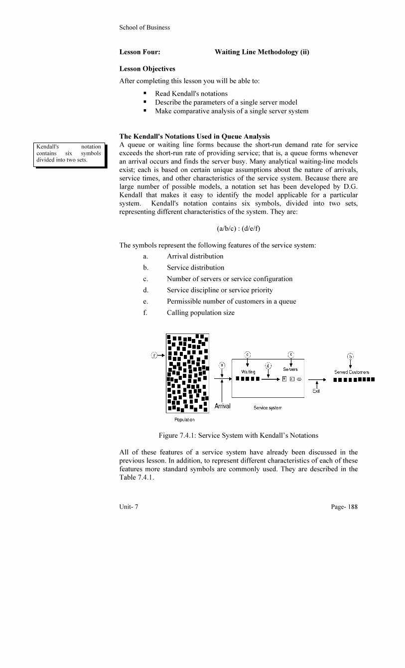
system. Kendall's notation contains six symbols, divided into two sets,
representing different characteristics of the system. They are:
(a/b/c) : (d/e/f)
The symbols represent the following features of the service system:
a. Arrival distribution
b. Service distribution
c. Number of servers or service configuration
d. Service discipline or service priority
e. Permissible number of customers in a queue
f. Calling population size
Figure 7.4.1: Service System with Kendall’s Notations
All of these features of a service system have already been discussed in the
previous lesson. In addition, to represent different characteristics of each of these
features more standard symbols are commonly used. They are described in the
Table 7.4.1.
Kendall's notation contains six symbols divided into two sets.
Bangladesh Open University
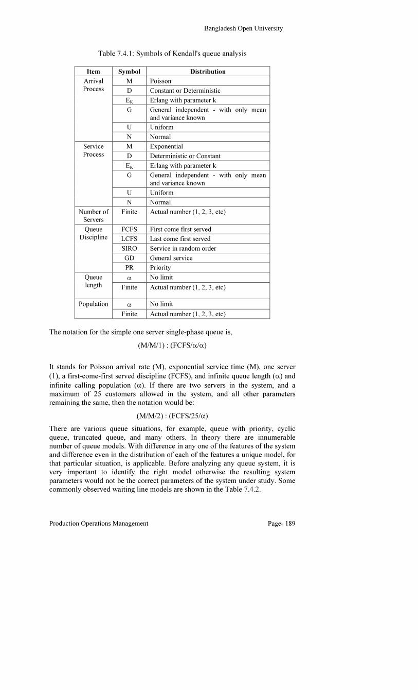
Production Operations Management Page- 189
Table 7.4.1: Symbols of Kendall's queue analysis
Item Symbol Distribution
Arrival
Process
M Poisson
D Constant or Deterministic
EK Erlang with parameter k
G General independent - with only mean
and variance known
U Uniform
N Normal
Service
Process
M Exponential
D Deterministic or Constant
EK Erlang with parameter k
G General independent - with only mean
and variance known
U Uniform
N Normal
Number of
Servers
Finite Actual number (1, 2, 3, etc)
Queue
Discipline
FCFS First come first served
LCFS Last come first served
SIRO Service in random order
GD General service
PR Priority
Queue
length
α No limit
Finite Actual number (1, 2, 3, etc)
Population
α No limit
Finite Actual number (1, 2, 3, etc)
The notation for the simple one server single-phase queue is,
(M/M/1) : (FCFS/α/α)
It stands for Poisson arrival rate (M), exponential service time (M), one server
(1), a first-come-first served discipline (FCFS), and infinite queue length (α) and
infinite calling population (α). If there are two servers in the system, and a
maximum of 25 customers allowed in the system, and all other parameters
remaining the same, then the notation would be:
(M/M/2) : (FCFS/25/α)
There are various queue situations, for example, queue with priority, cyclic
queue, truncated queue, and many others. In theory there are innumerable
number of queue models. With difference in any one of the features of the system
and difference even in the distribution of each of the features a unique model, for
that particular situation, is applicable. Before analyzing any queue system, it is
very important to identify the right model otherwise the resulting system
parameters would not be the correct parameters of the system under study. Some
commonly observed waiting line models are shown in the Table 7.4.2.
School of Business
Unit- 7 Page- 190
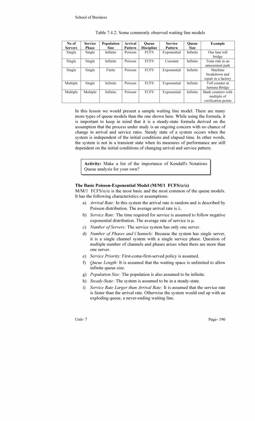
Table 7.4.2: Some commonly observed waiting line models
No of
Servers
Service
Phase
Population
Size
Arrival
Pattern
Queue
Discipline
Service
Pattern
Queue
Size
Example
Single Single Infinite Poisson FCFS Exponential Infinite One lane toll
bridge
Single Single Infinite Poisson FCFS Constant Infinite Train ride in an
amusement park
Single Single Finite Poisson FCFS Exponential Infinite Machine
breakdown and
repair in a factory
Multiple Single Infinite Poisson FCFS Exponential Infinite Toll counter at
Jamuna Bridge
Multiple Multiple Infinite Poisson FCFS Exponential Infinite Bank counters with
multiple of
verification points
In this lesson we would present a sample waiting line model. There are many
more types of queue models than the one shown here. While using the formula, it
is important to keep in mind that it is a steady-state formula derived on the
assumption that the process under study is an ongoing concern with no chance of
change in arrival and service rates. Steady state of a system occurs when the
system is independent of the initial conditions and elapsed time. In other words,
the system is not in a transient state when its measures of performance are still
dependent on the initial conditions of changing arrival and service pattern.
The Basic Poisson-Exponential Model (M/M/1 FCFS/α/α)
M/M/1 FCFS/α/α is the most basic and the most common of the queue models.
It has the following characteristics or assumptions:
a) Arrival Rate: In this system the arrival rate is random and is described by
Poisson distribution. The average arrival rate is λ.
b) Service Rate: The time required for service is assumed to follow negative
exponential distribution. The average rate of service is µ.
c) Number of Servers: The service system has only one server.
d) Number of Phases and Channels: Because the system has single server,
it is a single channel system with a single service phase. Question of
multiple number of channels and phases arises when there are more than
one server.
e) Service Priority: First-come-first-served policy is assumed.
f) Queue Length: It is assumed that the waiting space is unlimited to allow
infinite queue size.
g) Population Size: The population is also assumed to be infinite.
h) Steady-State: The system is assumed to be in a steady-state.
i) Service Rate Larger than Arrival Rate: It is assumed that the service rate
is faster than the arrival rate. Otherwise the system would end up with an
exploding queue, a never-ending waiting line.
Activity: Make a list of the importance of Kendall's Notations
Queue analysis for your own?
Bangladesh Open University
Production Operations Management Page- 191
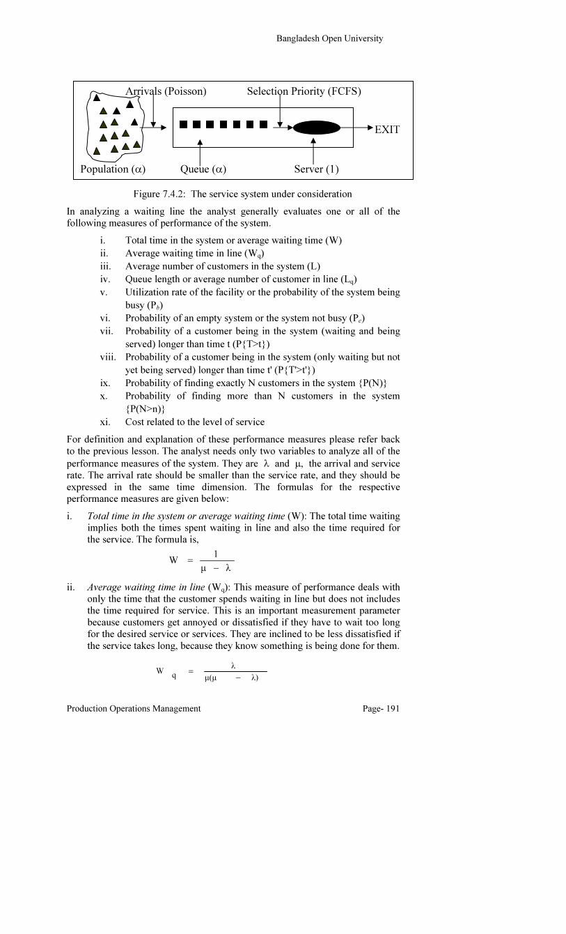
Figure 7.4.2: The service system under consideration
In analyzing a waiting line the analyst generally evaluates one or all of the
following measures of performance of the system.
i. Total time in the system or average waiting time (W)
ii. Average waiting time in line (Wq)
iii. Average number of customers in the system (L)
iv. Queue length or average number of customer in line (Lq)
v. Utilization rate of the facility or the probability of the system being
busy (Pb)
vi. Probability of an empty system or the system not busy (Pe)
vii. Probability of a customer being in the system (waiting and being
served) longer than time t (P{T>t})
viii. Probability of a customer being in the system (only waiting but not
yet being served) longer than time t' (P{T'>t'})
ix. Probability of finding exactly N customers in the system {P(N)}
x. Probability of finding more than N customers in the system
{P(N>n)}
xi. Cost related to the level of service
For definition and explanation of these performance measures please refer back
to the previous lesson. The analyst needs only two variables to analyze all of the
performance measures of the system. They are λ and µ, the arrival and service
rate. The arrival rate should be smaller than the service rate, and they should be
expressed in the same time dimension. The formulas for the respective
performance measures are given below:
i. Total time in the system or average waiting time (W): The total time waiting
implies both the times spent waiting in line and also the time required for
the service. The formula is,
ii. Average waiting time in line (Wq): This measure of performance deals with
only the time that the customer spends waiting in line but does not includes
the time required for service. This is an important measurement parameter
because customers get annoyed or dissatisfied if they have to wait too long
for the desired service or services. They are inclined to be less dissatisfied if
the service takes long, because they know something is being done for them.
λµ
1W
−
=
λ)µ(µ
λq
W−
=
Arrivals (Poisson) Selection Priority (FCFS)
EXIT
Population (α) Queue (α) Server (1)
School of Business
Unit- 7 Page- 192
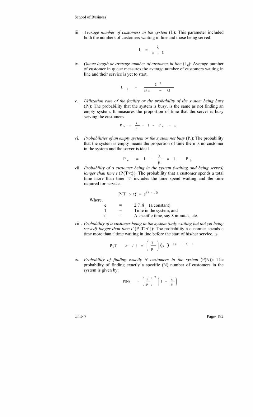
iii. Average number of customers in the system (L): This parameter included
both the numbers of customers waiting in line and those being served.
iv. Queue length or average number of customer in line (Lq): Average number
of customer in queue measures the average number of customers waiting in
line and their service is yet to start.
v. Utilization rate of the facility or the probability of the system being busy
(Pb): The probability that the system is busy, is the same as not finding an
empty system. It measures the proportion of time that the server is busy
serving the customers.
vi. Probabilities of an empty system or the system not busy (Pe): The probability
that the system is empty means the proportion of time there is no customer
in the system and the server is ideal.
vii. Probability of a customer being in the system (waiting and being served) longer than time t (P{T>t}): The probability that a customer spends a total
time more than time "t" includes the time spend waiting and the time
required for service.
Where,
e = 2.718 (a constant)
T = Time in the system, and
t = A specific time, say 8 minutes, etc.
viii. Probability of a customer being in the system (only waiting but not yet being served) longer than time t' (P{T'>t'}): The probability a customer spends a
time more than t' time waiting in line before the start of his/her service, is
ix. Probability of finding exactly N customers in the system (P(N)): The
probability of finding exactly a specific (N) number of customers in the
system is given by:
λ-µ
λL =
λ)µ(µ
λL
2
q−
=
ρP1µ
λP eb =−==
be P1µ
λ1P −=−=
( )tµ-λet}P{T =>
( ) t'λ)( µe
µ
λ}t'P{T'
−−
=>
−
=
µ
λ1
µ
λP(N)
N
Bangladesh Open University
Production Operations Management Page- 193
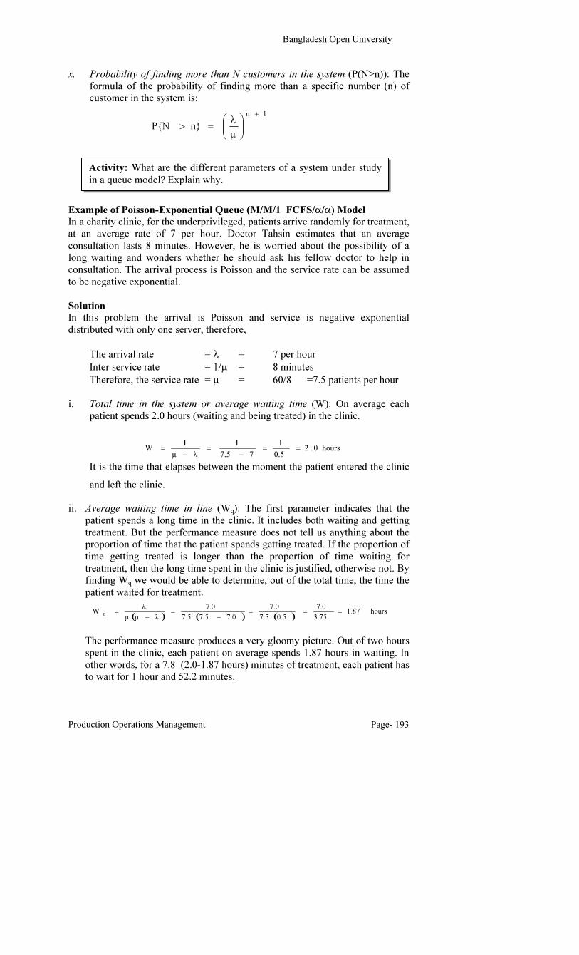
x. Probability of finding more than N customers in the system (P(N>n)): The
formula of the probability of finding more than a specific number (n) of
customer in the system is:
Example of Poisson-Exponential Queue (M/M/1 FCFS/α/α) Model
In a charity clinic, for the underprivileged, patients arrive randomly for treatment,
at an average rate of 7 per hour. Doctor Tahsin estimates that an average
consultation lasts 8 minutes. However, he is worried about the possibility of a
long waiting and wonders whether he should ask his fellow doctor to help in
consultation. The arrival process is Poisson and the service rate can be assumed
to be negative exponential.
Solution
In this problem the arrival is Poisson and service is negative exponential
distributed with only one server, therefore,
The arrival rate = λ = 7 per hour
Inter service rate = 1/µ = 8 minutes
Therefore, the service rate = µ = 60/8 =7.5 patients per hour
i. Total time in the system or average waiting time (W): On average each
patient spends 2.0 hours (waiting and being treated) in the clinic.
It is the time that elapses between the moment the patient entered the clinic
and left the clinic.
ii. Average waiting time in line (Wq): The first parameter indicates that the
patient spends a long time in the clinic. It includes both waiting and getting
treatment. But the performance measure does not tell us anything about the
proportion of time that the patient spends getting treated. If the proportion of
time getting treated is longer than the proportion of time waiting for
treatment, then the long time spent in the clinic is justified, otherwise not. By
finding Wq we would be able to determine, out of the total time, the time the
patient waited for treatment.
The performance measure produces a very gloomy picture. Out of two hours
spent in the clinic, each patient on average spends 1.87 hours in waiting. In
other words, for a 7.8 (2.0-1.87 hours) minutes of treatment, each patient has
to wait for 1 hour and 52.2 minutes.
1n
µ
λn}P{N
+
=>
hours 0.20.5
1
77.5
1
λµ
1W ==
−
=
−
=
( ) ( ) ( )hours1.87
3.75
7.0
0.57.5
7.0
7.07.57.5
7.0
λµµ
λW
q===
−
=
−
=
Activity: What are the different parameters of a system under study
in a queue model? Explain why.
School of Business
Unit- 7 Page- 194
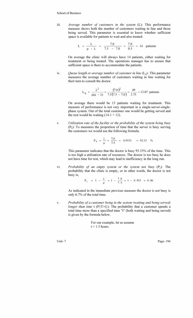
iii. Average number of customers in the system (L): This performance
measure shows both the number of customers waiting in line and those
being served. This parameter is essential to know whether sufficient
space is available for patients to wait and also treated.
On average the clinic will always have 14 patients, either waiting for
treatment or being treated. The operations manager has to ensure that
sufficient space is there to accommodate the patients.
iv. Queue length or average number of customer in line (Lq): This parameter
measures the average number of customers waiting in line waiting for
their turn to consult the doctor.
On average there would be 13 patients waiting for treatment. This
measure of performance is not very important in a single-server-single-
phase system. Out of the total customer one would be getting served and
the rest would be waiting (14-1 = 13).
v. Utilization rate of the facility or the probability of the system being busy
(Pb): To measures the proportion of time that the server is busy serving
the customers we would use the following formula.
This parameter indicates that the doctor is busy 93.33% of the time. This
is too high a utilization rate of resources. The doctor is too busy he does
not have time for rest, which may lead to inefficiency in the long run.
vi. Probability of an empty system or the system not busy (Pe): The
probability that the clinic is empty, or in other words, the doctor is not
busy is,
As indicated in the immediate previous measure the doctor is not busy is
only 6.7% of the total time.
v. Probability of a customer being in the system (waiting and being served)
longer than time t (P{T>t}): The probability that a customer spends a
total time more than a specified time "t" (both waiting and being served)
is given by the formula below.
For our example, let us assume
t = 1.5 hours
patients140.5
7.0
7.07.5
7.0
λ-µ
λL ==
−
==
( )( )
patients13.073.75
49
7.07.57.5
7.0
λ)µ(µ
λL
22
q ==
−
=
−
=
%93.330.93337.5
7.0
µ
λP b ====
06.0933.015.7
0.711P
e=−=−=−=
µ
λ
Bangladesh Open University
Production Operations Management Page- 195
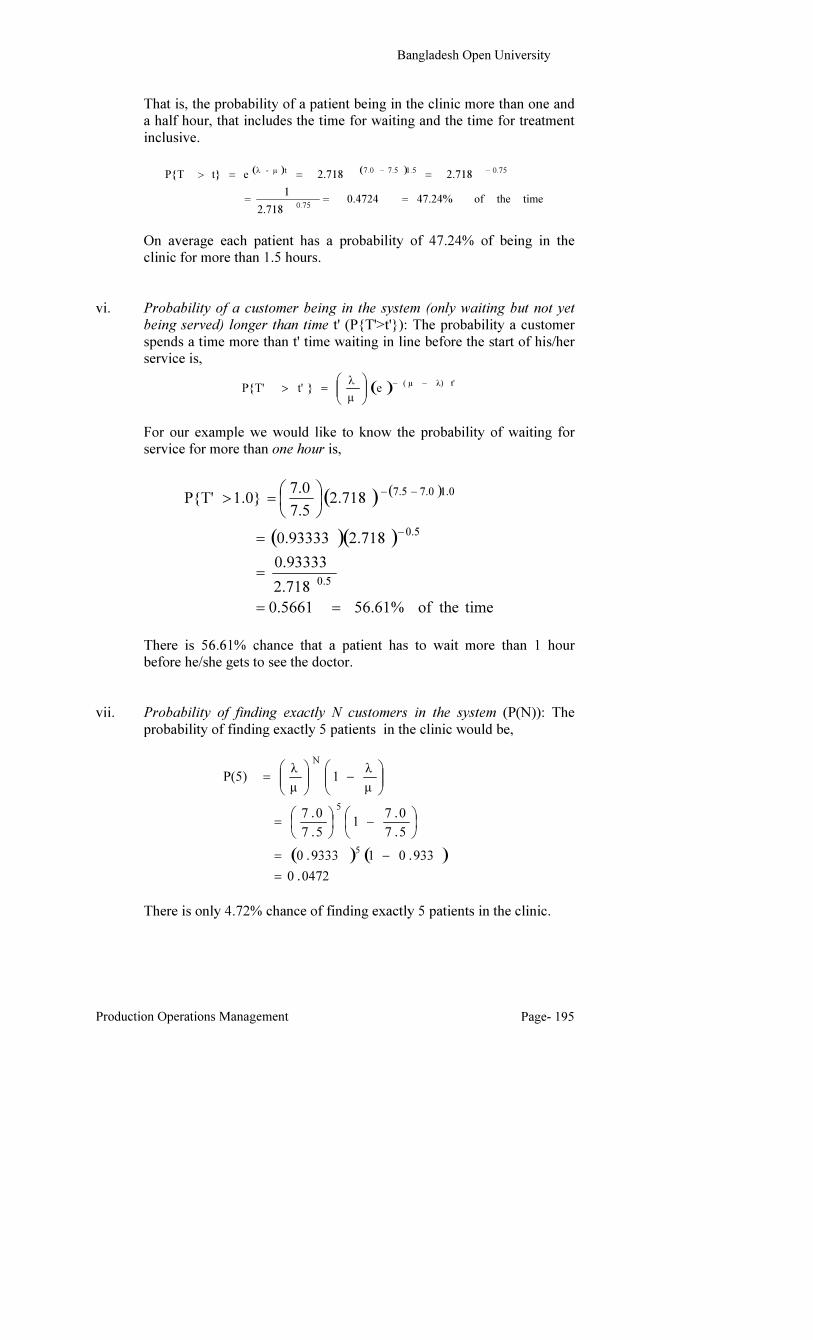
That is, the probability of a patient being in the clinic more than one and
a half hour, that includes the time for waiting and the time for treatment
inclusive.
On average each patient has a probability of 47.24% of being in the
clinic for more than 1.5 hours.
vi. Probability of a customer being in the system (only waiting but not yet
being served) longer than time t' (P{T'>t'}): The probability a customer
spends a time more than t' time waiting in line before the start of his/her
service is,
For our example we would like to know the probability of waiting for
service for more than one hour is,
There is 56.61% chance that a patient has to wait more than 1 hour
before he/she gets to see the doctor.
vii. Probability of finding exactly N customers in the system (P(N)): The
probability of finding exactly 5 patients in the clinic would be,
There is only 4.72% chance of finding exactly 5 patients in the clinic.
( ) ( )
timetheof47.24%0.47242.718
1
2.7182.718et}P{T
0.75
0.751.57.57.0tµ-λ
===
===>−−
( ) t'λ)( µe
µ
λ}t'P{T'
−−
=>
( ) ( )
0472.0
933.019333.0
5.7
0.71
5.7
0.7
µ
λ1
µ
λP(5)
5
5
N
=
−=
−
=
−
=
( ) ( )
( )( )
timetheof56.61%0.5661
2.718
0.93333
2.7180.93333
2.7187.5
7.01.0} P{T'
0.5
0.5
1.07.07.5
==
=
=
=>
−
−−
School of Business
Unit- 7 Page- 196
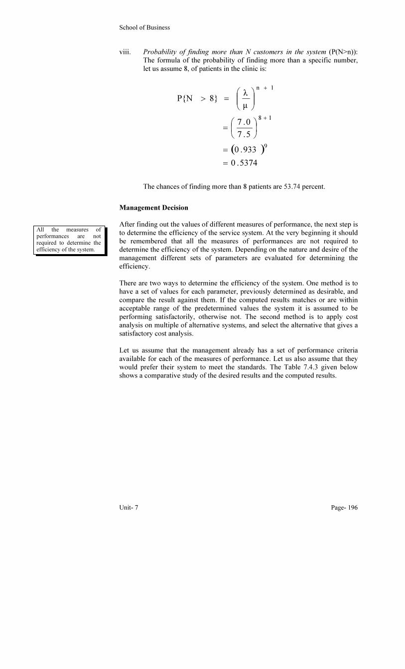
viii. Probability of finding more than N customers in the system (P(N>n)):
The formula of the probability of finding more than a specific number,
let us assume 8, of patients in the clinic is:
The chances of finding more than 8 patients are 53.74 percent.
Management Decision
After finding out the values of different measures of performance, the next step is
to determine the efficiency of the service system. At the very beginning it should
be remembered that all the measures of performances are not required to
determine the efficiency of the system. Depending on the nature and desire of the
management different sets of parameters are evaluated for determining the
efficiency.
There are two ways to determine the efficiency of the system. One method is to
have a set of values for each parameter, previously determined as desirable, and
compare the result against them. If the computed results matches or are within
acceptable range of the predetermined values the system it is assumed to be
performing satisfactorily, otherwise not. The second method is to apply cost
analysis on multiple of alternative systems, and select the alternative that gives a
satisfactory cost analysis.
Let us assume that the management already has a set of performance criteria
available for each of the measures of performance. Let us also assume that they
would prefer their system to meet the standards. The Table 7.4.3 given below
shows a comparative study of the desired results and the computed results.
( )
5374.0
933.0
5.7
0.7
µ
λ8}P{N
9
18
1n
=
=
=
=>
+
+
All the measures of performances are not required to determine the efficiency of the system.
Bangladesh Open University
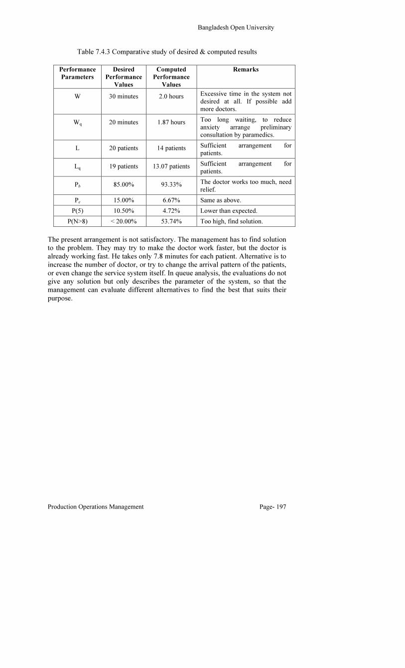
Production Operations Management Page- 197
Table 7.4.3 Comparative study of desired & computed results
Performance
Parameters
Desired
Performance
Values
Computed
Performance
Values
Remarks
W 30 minutes 2.0 hours Excessive time in the system not
desired at all. If possible add
more doctors.
Wq 20 minutes 1.87 hours Too long waiting, to reduce
anxiety arrange preliminary
consultation by paramedics.
L 20 patients 14 patients Sufficient arrangement for
patients.
Lq 19 patients 13.07 patients Sufficient arrangement for
patients.
Pb 85.00% 93.33% The doctor works too much, need
relief.
Pe 15.00% 6.67% Same as above.
P(5) 10.50% 4.72% Lower than expected.
P(N>8) < 20.00% 53.74% Too high, find solution.
The present arrangement is not satisfactory. The management has to find solution
to the problem. They may try to make the doctor work faster, but the doctor is
already working fast. He takes only 7.8 minutes for each patient. Alternative is to
increase the number of doctor, or try to change the arrival pattern of the patients,
or even change the service system itself. In queue analysis, the evaluations do not
give any solution but only describes the parameter of the system, so that the
management can evaluate different alternatives to find the best that suits their
purpose.
School of Business
Unit- 7 Page- 198
Discussion Questions
1. Describe the different symbols of Kendall’s notation.
2. During the height of the construction season in Rajshahi, trucks arrive at a
brick-field according to Poisson distribution at the rate of 26 trucks per hour.
The present capacity of the brick-field permits loading of 32 trucks per hour.
The service rate has exponential density function. Find
a) The average length of time a truck would be in the brick-field.
b) The proportion of time the brick-field is empty of trucks.
c) The probability of waiting more than 15 minutes.
d) The probability of finding more than 6 trucks in the brick-field.
e) If the service capacity decreases to 30 trucks per hour what would be
its effect on the average waiting time for each truck.
3. The manager of a neighborhood store is interested in providing good service
to the customers of his store. Presently, the store has a checkout counter for
the customers. On average, 30 customers arrive at the counter every hour,
according to Poisson distribution, and are served at an average rate of 35
customers per hour, with exponential service time. Find the following
averages:
a) Utilization of the checkout clerk.
b) Number of customers in the system.
c) Number of customers in line.
d) Time spent by the customer in store.
e) Waiting time in line.
4. A plant distributes its products by trucks. The average loading time is 20
minutes per truck. Trucks arrive at an average rate of two each hour.
Management feels that the existing loading facility is more than adequate.
However, the drivers complain that they have to wait too long. Analyze the
situation and find how much money the company can save by speeding up
loading if the waiting time of a truck is figured at Taka 250 per hour and the
plant operates eight hour each day.
Bangladesh Open University
Production Operations Management Page- 199
Conquering Those Killer Queues
By: N. R. Kleinfeld
Lines are one of Richard Larson’s odd fascinations. He is a steadfastly gleeful
professor of electrical engineering and computer science at the Massachusetts
Institute of Technology, and something of an expert on waiting. Thus the Zayre
Corporation, whose discount prices make it something of an expert on making
people wait, has hired him to come up with fresh ideas to combat that
immemorial bagaboo – customer lines.
Eugene Fram, a professor of marketing and management at the Rochester
Institute of Technology, feels that businesses are recognizing that by keeping
customers waiting they become “time bandits.” They are finding that people will
pick one establishment over another because of shorter lines. All this means more
pressure on companies – from bank to restaurants, supermarkets to airlines – to
solve the waiting problem. There are quick cures: spend more money and provide
more service. But most businesses cannot afford to – or do not want to – and so
they have been trying harder to find imaginative methods to curtail waiting or at
least make it less repugnant.
Those who wrestle with waiting often contact someone like Richard Larson.
More and more researchers and consultants are studying lines and, in their efforts
to demystify and quantify them, have produced a mathematical discipline.
Queuing theory makes heavy use of probability theory and gets into abstruse
mathematical equations that gauge such things as how many people will arrive at
a drugstore to buy dental floss during the noon hour.
The father of queuing theory is A. K. Erlang, a Danish telephone engineer who,
in 1908, began to study congestion in the telephone service of the Copenhagen
Telephone Company. A few years later, he arrived at a mathematical approach to
assist in designing telephone switches. Queuing theory has grown far more
sophisticated. While it continues to have its chief application in
telecommunications and computer design, it has seeped elsewhere.
Ideas about lines matter to the people at Zayre, because they have tried to
differentiate their store from competitors I part by how swiftly they take
customers’ money. For years, Zayre has had a policy that if more than three
people are lined up at a checkout register, another register will open.
The system, Zayre admits, has its flaws. Lines do occasionally swell to four or
five customers when no one is free to handle another register. At times, every
register is open and yet the lines are four deep. “We found the system was
difficult to manage, because it was hard to predict when customers would arrive,:
said Frank Capek, Zayre’s manager of operations planning.
Years of listening to howling customers have also taught the airlines some
baggage-retrieval lessons. When American designed its baggage-claim area in
Dallas-Fort Worth Airport, it put it close to the gates, so disembarking passengers
would not have to trudge too far. But even though passengers reach the area
quickly, they must wait for their luggage. At Los Angeles International Airport,
passengers have to walk quite some distance to the claim area, but when they
Case
Analysis
School of Business
Unit- 7 Page- 200
arrive, their suitcases are usually there. Even though the Los Angeles travelers
spend more total time picking up their baggage, American has found they do not
grouse as much about baggage delays as do the Dallas passengers.
Few businesses have taken more hard shots about bad management of lines than
banks. “Our research indicates that people don’t like to spend time in bank
branches,” said David Mooney, senior vice president of Chemical Bank. “It’s
probably second in their disdain to waiting to see the dentist.”
To reduce lines, most banks have installed automatic teller machines and tried to
persuade employers to alter their check distribution or to directly deposit payroll
checks in the bank. The lines, however, persist.
One way to take some of the stings out of waiting is to entertain customers. Since
1959, the Manhattan Savings Bank has offered live entertainment during the
frenzied noontime hours. In 13 branches, a pianist performs and one branch has
an organ player (Willard Denton, the former Chemical chairman who dreamed up
the idea, liked organs, though present management thinks they are a trifle loud
for a bank). Occasionally, to make line-waiting even more wonderful, Manhattan
Savings has scheduled events such as a fancy-cat exhibit, a purebred dog show
and a boat show.
Because of all this, Manhattan Savings believes customers endure long waits
better than those who go to banks where the only music is the person in front of
you grinding his teeth. “At very hectic times, we get very few complaints,” said
Jean Madsen, a senior vice president.
At hotels and office buildings, mirrors affixed to elevator doors make people less
maniacal during waits. Instead of deciding whom to kill, they can comb their
hair. A study done by Russel Ackoff showed that hotels that had mirrors received
far less grumbling about elevator delays than ones without mirrors.
Just telling people how long they have to wait often cheers them up. Disneyland
is sensitive to waiting, since the line for a hot attraction like Star Tours can run to
1800 people. Like many amusement parks, Disney employs entertainment for
waiters, but it is also big on feedback. At various spots along lines, signs give
estimated delays from those points. Queuing experts say nothing is worse than
the blind waiting familiar to people at bus stops, who don’t know if the next bus
is one minute or 15 minutes away. Disney’s feedback permits parents to weigh
odd options: Is it wiser to wait 25 minutes fo rMr. Toad’s Wild Ride or 30
minutes for Dumbo?
Peter Kolesar, a professor of operations research at the Columbia University
Business School, thinks there ought to be more efforts to shift demand by altering
pricing. Some rail lines, for example, charge less for off-peak trains and
restaurants offer early-bird discounts.
During a whimsical moment, Dick Larson speculated that if the average
American waited hald an hour a day in one line or another, then the population
expended 37 billion hours a year in lines. It strikes him, he said, that businesses
ought to consider merchandising products to idle waiters to take their minds off
Bangladesh Open University
Production Operations Management Page- 201
pulling out their hair. “Like those flower peddlers outside tunnels and bridges,”
he said. “They are very shrewd.”
Case questions
1. What options might a chain store such as Zayre employ to increase
capacity? To influence demand? 2. What techniques can be employed to make a wait seem more pleasant
(besides the ones mentioned here)?
3. What products could be realistically merchandised?
Source: Excerpted from New York Times (Sunday, September 25, 1988)
Mentioned in the book “Service Operations Management” by Robert, G.
Murdick, Barry Render, and Roberta S. Russell, Prentice Hall, pages 344-345.