washington university sever institute of …jst/studenttheses/sshi... · the ip multicast solution...
TRANSCRIPT

WASHINGTON UNIVERSITY
SEVER INSTITUTE OF TECHNOLOGY
DEPARTMENT OF COMPUTER SCIENCE
DESIGN OF OVERLAY NETWORKS FOR INTERNET MULTICAST
by
Yunxi Sherlia Shi
Prepared under the direction of Professor Jonathan S. Turner
A dissertation presented to the Sever Institute of
Washington University in partial fulfillment
of the requirements for the degree of
Doctor of Science
August, 2002
Saint Louis, Missouri

WASHINGTON UNIVERSITY
SEVER INSTITUTE OF TECHNOLOGY
DEPARTMENT OF COMPUTER SCIENCE
ABSTRACT
DESIGN OF OVERLAY NETWORKS FOR INTERNET MULTICAST
by Yunxi Sherlia Shi
ADVISOR: Professor Jonathan S. Turner
August, 2002
Saint Louis, Missouri
Multicast is an efficient transmission scheme for supporting group communication
in networks. Contrasted with unicast, where multiple point-to-point connections must be
used to support communications among a group of users, multicast is more efficient be-
cause each data packet is replicated in the network – at the branching points leading to dis-
tinguished destinations, thus reducing the transmission load on the data sources and traffic
load on the network links. To implement multicast, networks need to incorporate new rout-
ing and forwarding mechanisms in addition to the existing unicast methods. Unfortunately,
the necessary functions needed to realize multicast are not adequately supported in the cur-
rent networks. The IP multicast solution has serious scaling and deployment limitations,
and cannot be easily extended to provide more enhanced data services. Furthermore, and

perhaps most importantly, IP multicast has ignored the economic nature of the problem,
lacking incentives for service providers to deploy the service in wide area networks.
Overlay multicast holds promise for the realization of large scale Internet multicast
services. An overlay network is a virtual topology constructed on top of the Internet infras-
tructure. The concept of overlay networks enables multicast to be deployed as a service
network rather than a network primitive mechanism, allowing deployment over heteroge-
neous networks without the need of universal network support. This dissertation addresses
the network design aspects of overlay networks to provide scalable multicast services in
the Internet. The resources and the network cost in the context of overlay networks are dif-
ferent from that in conventional networks, presenting new challenges and new problems to
solve. Our design goals are the maximization of network utility and improved service qual-
ity. As the overall network design problem is extremely complex, we divide the problem
into three components: the efficient management of session traffic (multicast routing), the
provisioning of overlay network resources (bandwidth dimensioning) and overlay topol-
ogy optimization (service placement). The combined solution provides a comprehensive
procedure for planning and managing an overlay multicast network.
We also consider a complementary form of overlay multicast called application-
level multicast (ALMI). ALMI allows end systems to directly create an overlay multicast
session among themselves. This gives applications the flexibility to communicate without
relying on service providers. The tradeoff is that users do not have direct control on the
topology and data paths taken by the session flows and will typically get lower quality of
service due to the best effort nature of the Internet environment. ALMI is therefore suitable
for sessions of small size or sessions where all members are well connected to the network.
Furthermore, the ALMI framework allows us to experiment with application specific com-
ponents such as data reliability, in order to identify a useful set of communication semantics
for enhanced data services.

To my grandmother

Contents
List of Tables . . . . . . . . . . . . . . . . . . . . . . . . . . . . . . . . . . . . vii
List of Figures . . . . . . . . . . . . . . . . . . . . . . . . . . . . . . . . . . . viii
Acknowledgments . . . . . . . . . . . . . . . . . . . . . . . . . . . . . . . . . x
1 Introduction . . . . . . . . . . . . . . . . . . . . . . . . . . . . . . . . . . . 1
1.1 Group Communications . . . . . . . . . . . . . . . . . . . . . . . . . . . . 1
1.2 A Brief History of Internet Multicast . . . . . . . . . . . . . . . . . . . . . 4
1.3 Why Overlay? . . . . . . . . . . . . . . . . . . . . . . . . . . . . . . . . . 6
1.4 Contributions . . . . . . . . . . . . . . . . . . . . . . . . . . . . . . . . . 8
1.5 Outline . . . . . . . . . . . . . . . . . . . . . . . . . . . . . . . . . . . . 10
2 Architecture of Overlay Multicast Networks . . . . . . . . . . . . . . . . . 11
2.1 Background on Internet Architecture . . . . . . . . . . . . . . . . . . . . . 11
2.2 Overview of Overlay Multicast Networks . . . . . . . . . . . . . . . . . . 16
2.3 Benefits of Overlay Multicast Networks . . . . . . . . . . . . . . . . . . . 20
2.4 Cost of Overlay Multicast Networks . . . . . . . . . . . . . . . . . . . . . 22
2.4.1 Evaluation Methodology . . . . . . . . . . . . . . . . . . . . . . . 26
2.4.2 Comparisons with Network Multicast Trees . . . . . . . . . . . . . 28
2.5 Overview of Design Issues . . . . . . . . . . . . . . . . . . . . . . . . . . 34
2.6 Related Work . . . . . . . . . . . . . . . . . . . . . . . . . . . . . . . . . 37
2.7 Summary . . . . . . . . . . . . . . . . . . . . . . . . . . . . . . . . . . . 39
3 Multicast Routing in Overlay Networks . . . . . . . . . . . . . . . . . . . . 40
3.1 Problem Definitions . . . . . . . . . . . . . . . . . . . . . . . . . . . . . . 42
3.2 Routing Algorithms: Greedy Approach . . . . . . . . . . . . . . . . . . . 45
3.2.1 The Compact Tree Algorithm . . . . . . . . . . . . . . . . . . . . 46
iv

3.2.2 The Balanced Compact Tree Algorithm . . . . . . . . . . . . . . . 49
3.3 Routing Algorithms: Balanced Degree Allocation . . . . . . . . . . . . . . 50
3.3.1 The Degree Allocation Problem . . . . . . . . . . . . . . . . . . . 52
3.3.2 Algorithms Based On Balanced Degree Allocation . . . . . . . . . 53
3.4 Cost of Overlay Trees Revisited . . . . . . . . . . . . . . . . . . . . . . . 57
3.4.1 Overlay Cost on Disk Configuration . . . . . . . . . . . . . . . . . 58
3.4.2 Overlay Cost on Metro Configuration . . . . . . . . . . . . . . . . 59
3.5 Related Work . . . . . . . . . . . . . . . . . . . . . . . . . . . . . . . . . 63
3.6 Summary . . . . . . . . . . . . . . . . . . . . . . . . . . . . . . . . . . . 64
4 Link Dimensioning and Evaluation of Routing Algorithms . . . . . . . . . 66
4.1 Access Bandwidth Dimensioning . . . . . . . . . . . . . . . . . . . . . . . 67
4.1.1 Baseline Dimensioning . . . . . . . . . . . . . . . . . . . . . . . . 68
4.1.2 Iterative Dimensioning . . . . . . . . . . . . . . . . . . . . . . . . 70
4.2 Evaluation of the Routing Algorithms . . . . . . . . . . . . . . . . . . . . 71
4.2.1 Simulation Setup . . . . . . . . . . . . . . . . . . . . . . . . . . . 71
4.2.2 Comparison of Tree Building Techniques . . . . . . . . . . . . . . 73
4.2.3 Performance Comparison on Session Rejection Rate . . . . . . . . 75
4.2.4 Performance Comparison on Multicast Tree Diameter . . . . . . . 78
4.3 Handling Dynamic Sessions . . . . . . . . . . . . . . . . . . . . . . . . . 79
4.4 A Hybrid Scheme To Reduce Complexity . . . . . . . . . . . . . . . . . . 84
4.5 Implementation Cost . . . . . . . . . . . . . . . . . . . . . . . . . . . . . 85
4.6 Summary . . . . . . . . . . . . . . . . . . . . . . . . . . . . . . . . . . . 87
5 Placing Servers in Overlay Networks . . . . . . . . . . . . . . . . . . . . . 89
5.1 Formal definitions and the Algorithms . . . . . . . . . . . . . . . . . . . . 92
5.1.1 LP Relaxation-based Methods . . . . . . . . . . . . . . . . . . . . 93
5.1.2 Greedy Heuristics . . . . . . . . . . . . . . . . . . . . . . . . . . . 95
5.1.3 Comparison of the FR, IR and the Greedy Algorithms . . . . . . . 95
5.2 Network Models . . . . . . . . . . . . . . . . . . . . . . . . . . . . . . . 96
5.3 Simulation Results . . . . . . . . . . . . . . . . . . . . . . . . . . . . . . 100
5.3.1 Single Network . . . . . . . . . . . . . . . . . . . . . . . . . . . . 100
5.3.2 Multiple Networks . . . . . . . . . . . . . . . . . . . . . . . . . . 103
5.3.3 Server Load . . . . . . . . . . . . . . . . . . . . . . . . . . . . . . 106
5.4 Related Work . . . . . . . . . . . . . . . . . . . . . . . . . . . . . . . . . 107
v

5.5 Summary . . . . . . . . . . . . . . . . . . . . . . . . . . . . . . . . . . . 109
6 Multicast Service in End-systems . . . . . . . . . . . . . . . . . . . . . . . 110
6.1 Architecture Overview . . . . . . . . . . . . . . . . . . . . . . . . . . . . 112
6.2 Protocols and Operations . . . . . . . . . . . . . . . . . . . . . . . . . . . 114
6.2.1 Session Membership Operations . . . . . . . . . . . . . . . . . . . 118
6.2.2 Multicast Tree Management . . . . . . . . . . . . . . . . . . . . . 120
6.3 Application-Specific Components . . . . . . . . . . . . . . . . . . . . . . 122
6.3.1 End to End Data Reliability . . . . . . . . . . . . . . . . . . . . . 122
6.3.2 Data Naming . . . . . . . . . . . . . . . . . . . . . . . . . . . . . 125
6.3.3 Other Components . . . . . . . . . . . . . . . . . . . . . . . . . . 126
6.4 Experimental Evaluation . . . . . . . . . . . . . . . . . . . . . . . . . . . 126
6.4.1 Experiment Over WAN . . . . . . . . . . . . . . . . . . . . . . . . 127
6.4.2 Experiment Over LAN . . . . . . . . . . . . . . . . . . . . . . . . 129
6.5 Related Work . . . . . . . . . . . . . . . . . . . . . . . . . . . . . . . . . 130
6.6 Summary . . . . . . . . . . . . . . . . . . . . . . . . . . . . . . . . . . . 131
7 Conclusion . . . . . . . . . . . . . . . . . . . . . . . . . . . . . . . . . . . 133
7.1 Contributions . . . . . . . . . . . . . . . . . . . . . . . . . . . . . . . . . 133
7.2 Future Work . . . . . . . . . . . . . . . . . . . . . . . . . . . . . . . . . . 136
7.3 Final Remarks . . . . . . . . . . . . . . . . . . . . . . . . . . . . . . . . . 137
References . . . . . . . . . . . . . . . . . . . . . . . . . . . . . . . . . . . . . 138
Vita . . . . . . . . . . . . . . . . . . . . . . . . . . . . . . . . . . . . . . . . . 147
vi

List of Tables
1.1 Application Characteristics for Group Communication . . . . . . . . . . . 3
3.1 Summary of the Overlay Multicast Trees . . . . . . . . . . . . . . . . . . . 57
5.1 Parameters for Generating Network Graphs . . . . . . . . . . . . . . . . . 97
5.2 Average Client to Server distance . . . . . . . . . . . . . . . . . . . . . . . 103
5.3 Number of Peering Links In Use . . . . . . . . . . . . . . . . . . . . . . . 103
6.1 Experiment of ALMI Forwarding Delay in End Systems . . . . . . . . . . 129
vii

List of Figures
2.1 Route Trace of Peering between Southwestern Bell Network and Verio Net-
work . . . . . . . . . . . . . . . . . . . . . . . . . . . . . . . . . . . . . . 14
2.2 Efficient Routes Enabled by Direct Network Peerings . . . . . . . . . . . . 15
2.3 Overview of AMcast Architecture . . . . . . . . . . . . . . . . . . . . . . 17
2.4 An Example of the Mapping between Network Topology and AMcast Vir-
tual Tree Topology . . . . . . . . . . . . . . . . . . . . . . . . . . . . . . 23
2.5 Disk and Metro Network Topology . . . . . . . . . . . . . . . . . . . . . . 27
2.6 Tree Comparison on Disk Configuration . . . . . . . . . . . . . . . . . . . 30
2.7 Tree Comparison on Metro Configuration . . . . . . . . . . . . . . . . . . 33
3.1 Trade-off Of Multicast Routing Parameters: End-to-end Delay and Access
Bandwidth. . . . . . . . . . . . . . . . . . . . . . . . . . . . . . . . . . . 41
3.2 An Example of the Compact Tree Algorithm . . . . . . . . . . . . . . . . . 47
3.3 The CT Heuristic Algorithm for MDDL . . . . . . . . . . . . . . . . . . . 48
3.4 An Example of the ICT Algorithm with Degree Adjustment . . . . . . . . . 56
3.5 Comparison of Overlay and Network Multicast Trees Over Disk Configu-
ration . . . . . . . . . . . . . . . . . . . . . . . . . . . . . . . . . . . . . 58
3.6 Comparison of Overlay and Network Multicast Trees Over Metro Config-
uration . . . . . . . . . . . . . . . . . . . . . . . . . . . . . . . . . . . . . 60
3.7 Pairwise Delay Performance of Overlay Trees . . . . . . . . . . . . . . . . 61
4.1 Dimension of Server Access Bandwidth . . . . . . . . . . . . . . . . . . . 69
4.2 Convergence of Iterative Bandwidth Dimensioning . . . . . . . . . . . . . 71
4.3 Effect of Total Dimensioned Bandwidth . . . . . . . . . . . . . . . . . . . 71
4.4 Overlay Network Configurations . . . . . . . . . . . . . . . . . . . . . . . 72
4.5 Sensitivity to Diameter Bound . . . . . . . . . . . . . . . . . . . . . . . . 74
4.6 Sensitivity to Degree Adjustment Round . . . . . . . . . . . . . . . . . . . 74
viii

4.7 Rejection Fraction Comparison . . . . . . . . . . . . . . . . . . . . . . . . 76
4.8 Routing Performance over Differently Dimensioned Networks . . . . . . . 77
4.9 End-to-end Delay performance . . . . . . . . . . . . . . . . . . . . . . . . 79
4.10 Performance with Even Number of Join and Leave Requests . . . . . . . . 81
4.11 Effect of Dynamic Join Requests . . . . . . . . . . . . . . . . . . . . . . . 82
4.12 Effect of Dynamic Leave Requests . . . . . . . . . . . . . . . . . . . . . . 82
4.13 Performance with Tree Re-arrangement . . . . . . . . . . . . . . . . . . . 83
4.14 Computation Complexity of the ICT Algorithm . . . . . . . . . . . . . . . 84
4.15 Performance of the hybrid CP and CT Algorithms . . . . . . . . . . . . . . 85
4.16 Trade-off between Network Operating Load and Routing Update Frequency. 86
4.17 Percentage of Re-routed Sessions . . . . . . . . . . . . . . . . . . . . . . . 86
5.1 Performance Comparison of the FR and IR Algorithms . . . . . . . . . . . 96
5.2 Variation on Server Service Range . . . . . . . . . . . . . . . . . . . . . . 101
5.3 Variation on Different Service Requirement . . . . . . . . . . . . . . . . . 102
5.4 Variation on Network Peering Density . . . . . . . . . . . . . . . . . . . . 104
5.5 Relative Performance Ratio Against Lower Bound . . . . . . . . . . . . . . 105
5.6 Characteristics of Server Load . . . . . . . . . . . . . . . . . . . . . . . . 106
6.1 ALMI Architecture Overview . . . . . . . . . . . . . . . . . . . . . . . . 112
6.2 ALMI Packet Header Format . . . . . . . . . . . . . . . . . . . . . . . . . 115
6.3 ALMI Components Architecture . . . . . . . . . . . . . . . . . . . . . . . 117
6.4 ALMI Naming and Error Control . . . . . . . . . . . . . . . . . . . . . . . 123
6.5 Example WAN Topology (Path delay measured from traceroute) . . . . . . 127
6.6 Evaluation of ALMI MST in WAN Test . . . . . . . . . . . . . . . . . . . 128
ix

Acknowledgments
My foremost thank goes to my thesis adviser Dr. Jonathan Turner. Without him, this dis-sertation would not have been possible. I thank him for his patience and encouragementthat carried me on through difficult times, and for his insights and suggestions that helpedto shape my research skills. His valuable feedback contributed greatly to this dissertation.
I am grateful to my former adviser Dr. Guru Parulkar, who introduced and helpedme to start my graduate student life in Computer Science. His visionary thoughts andenergetic working style have influenced me greatly as a computer scientist.
I also thank Dr. Marcel Waldvogel, who advised me and helped me in various as-pects of my research. He is the one that I can always count on to discuss the tiniest detailsof a problem, and that knows all the computer tools inside-out and has the longest .emacsfile I have ever seen.
I thank the rest of my thesis committee members: Dr. Roger Chamberlain, Dr. KenGoldman, and Dr. Weixiong Zhang. Their valuable feedback helped me to improve thedissertation in many ways.
I thank all the students and staffs in ARL and the Computer Science department,whose presences and fun-loving spirits made the otherwise grueling experience tolerable.They are: Sumi Choi, John Dehart, Anshul Kantawala, Fred Kuhns, Qingfeng Huang, Sam-phel Norden, Prashanth Pappu, Ruibiao Qiu, Jai Ramamirtham, Ed Spitznagel, David Tay-lor, Tilman Wolf, Ken Wong and Yan Zhou. I also thank the former g-troup members:Milind Buddhikot, Girish Chandranmenon, Chuck Cranor, Dan Decasper, Zubin Dittia,R. Gopal and Christos Papadopoulos. I enjoyed all the vivid discussions we had on varioustopics and had lots of fun being a member of this fantastic group.
Last but not least, I thank my grandmother, my parents and my sister for alwaysbeing there when I needed them most, and for supporting me through all these years.
Sherlia Shi
Washington University in Saint LouisAugust 2002
x

1
Chapter 1
Introduction
This dissertation presents a new service network architecture for providing multicast ser-
vices in the Internet and offers comprehensive solutions to the issues of designing the ser-
vice network from a service provider’s perspective. The premise of this work is that mul-
ticast services, as a fundamental communication model of human interactions, ought to be
implemented at a higher service layer, not as a network primitive. This allows the multicast
service to be provided over diversified networks, and allows more flexibility in the service
models, as they can be tailored to the needs of applications.
1.1 Group Communications
With the enormous advances in network computing and communication technologies, the
Internet has become essential for information exchange in many parts of the world today.
Yet, today’s web and email based networking is just the beginning of an upcoming in-
formation age, with the ultimate technology wave still preparing its entrance. The next
generation of the Internet will ride on the vast progress on network infrastructure, which
enables two important advances. First, it enables high speed real-time multimedia appli-
cations to be carried over the commodity Internet; Second, broadband access reaches to
millions of households enabling person-to-person network communications in a cheaper
and better way.

Chapter 1. Introduction 2
However, today’s computer-supported communication is largely limited to data ex-
change between two computers, or point-to-point communications. Group communication,
on the other hand, is minimally supported, even though it is an equally important and natu-
ral model of communication in people’s day-to-day experiences. Students going to classes,
professionals going to staff meetings, friends getting together watching a game, are all dif-
ferent forms of group communication. Unfortunately, most of these applications are still
little developed or are only supported in very limited scales. This lack of support coin-
cides with the limited and expensive network infrastructure we have today, but as stated
earlier, this will change shortly and the availability of rich-media network communication
and high-speed network access for households and business corporations, with the appro-
priate development of applications, will drive the demand for system and network support
for group communications.
Multicast is an efficient transmission mechanism that supports group communica-
tion semantics. In contrast to point-to-point transmission, or unicast, in which a data source
sends a copy of data to each of the receivers, a multicast data source only sends one copy
of data which is replicated as necessary when propagating in the network towards the re-
ceivers. This is extremely helpful for small and less capable devices to disseminate data
to a large set of receivers, since the intelligence in the network helps the source to reduce
the load on both its CPU and its access link. Scalability is another reason for interest in
multicast, as it reduces the amount of total traffic injected into the network by each mul-
ticast session. This allows multicast to scale to very large group sizes and enables group
communication without traffic explosion in the network as in the case of unicast.
There is a diverse range of applications that inherently require group communica-
tion and collaboration: video conferencing, distance learning, distributed databases, data
replication, multi-party games and distributed simulation, network broadcast services and
many others. The diversity of these applications demands versatile support from the un-
derlying system in many dimensions. Examples of these dimensions include the amount
of data that needs to be delivered (bandwidth requirement), the timeliness of their delivery

Chapter 1. Introduction 3
(latency requirement), the reliability of their delivery (reliability requirement), the num-
ber of participants that send data (multi-source requirement), the number of recipients to
be reached (scalability requirement), and the frequency of members joining or leaving the
group (dynamics requirement). Table 1.1 summarizes the individual characteristics of sev-
eral next-generation applications.
Table 1.1: Application Characteristics for Group CommunicationMulti-source Scalability Dynamics Bandwidth Latency Reliability
VideoConference
all small low medium critical no
DistanceLearning
one or few medium low medium critical no
DistributedCache Update
few or all medium low high non-critical
yes
Multi-partyGames
all large high low critical yes
DistributedSimulation
all large low high depends yes
Peer-to-peer few huge high low non-critical
yes
InternetTV/Broadcast
one huge high high critical no
Supporting these applications has imposed a serious challenge to our current com-
munication systems. Due to the prevalence of underlying point-to-point connectivities,
communication systems are quickly reaching their limit. A typical example is that requests
to a popular web server usually experience long response time due to server overload since
it has to establish individual connections for each incoming data request, even for requests
for the same objects. The inadequacy of unicast-only systems is more significant for these
forward-looking applications, especially in distributed systems where data needs to be con-
stantly updated and synchronized.

Chapter 1. Introduction 4
1.2 A Brief History of Internet Multicast
In the early 80s, multicast was mostly restricted to the LAN environment, as it is well
supported by most local area network technologies, such as Ethernet and Token Rings.
On the other hand, extended LANs interconnected with bridges and inter-networks did
not support multicast data delivery. Although multicast addressing was designed from the
beginning as a separate address class in the IP address family, there were no standard ways
to use it. It was not until the late 80s that Deering introduced multicast extensions to
the unicast routing mechanisms across datagram-based inter-networks [19], marking the
beginning of IP multicast.
Following Deering’s work, the Multicast Backbone (MBone) [21] was born and
marked the first widespread use of multicast in the Internet. The MBone consists of tunnels
whose end points are workstations that implement the Distance Vector Multicast Routing
Protocol (DVMRP) [4] and are able to process unicast-encapsulated multicast packets and
then forward the packets to the appropriate outgoing interfaces computed by the routing
protocol. In March 1992, the MBone carried its first event with 20 sites worldwide received
multicast audio streams from a meeting of the Internet Engineering Task Force (IETF) in
San Diego.
However, DVMRP is inherently unscalable due to its “flood and prune” mechanism
for building the multicast tree. In DVMRP, each router discovers the existence of group
members by periodically issuing Internet Group Management Protocol (IGMP) queries.
Upon receiving the query, a leaf router will send a prune message indicating that it does not
have directly attached group members. An intermediate router forwards the prune message
towards the source if it receives prune messages on all its interfaces except the interface
towards the source. Such a mechanism requires that every router that supports multicast to
keep state for each existing multicast group, regardless if the router itself actually belongs
to the group tree or not. Thus DVMRP is also referred to as the dense mode protocol, as it
assumes the dense spreading of group members where pruning is scarce.

Chapter 1. Introduction 5
With the growth of MBone and the appearance of native mode multicast, i.e. routers
directly support multicast, the inefficiency of dense mode multicast routing protocols has to
be addressed. This motivates a new class of multicast routing protocols – the sparse mode
multicast routing protocols. The most widely implemented sparse mode protocol is the
Protocol Independent Multicast Sparse Mode (PIM-SM) [22]. Although PIM-SM avoids
some complexity of DVMRP, it also introduces many other issues that, to this date, are not
adequately solved [1].
Furthermore, in spite of the rigorous efforts of a generation of researchers, there
remains many unresolved issues in the IP multicast model that hinder the development and
deployment of IP multicast and multicast applications. The most prominent issues are the
lack of a multicast address allocation scheme, the lack of access control and the lack of an
inter-domain multicast routing protocol. A flexible and scalable address allocation scheme
is critical to the development of any multicast applications as it allows the quick discovery
of an multicast address available for immediate use. However, such scheme is not easily
devisable in a flat multicast address space, where each IP multicast address is a 32-bit
number (in the range of 224.0.0.0 to 239.255.255.255) with no geographical or topological
meaning. Consequently, most multicast applications randomly pick a multicast address and
hope that it is not currently in use. The possibility of address conflicts increases with the
number of multicast groups and complicates the applications unnecessarily.
Second, the lack of access control raises increasing concerns with the recent wave
of Distributed Denial of Service (DDOS) attacks [47]. In the IP multicast model, any ma-
chine can send to a multicast address without registering itself with the group. Until the
IGMPv3 [8], a multicast receiver had no means of selecting the data sources to receive
packets from; by default, all packets sent to a multicast address are forwarded to all re-
ceivers. In IGMPv3, source filters are added to allow receivers to specify the sources they
wish to listen to or specify all but those they don’t wish to listen to, provided that receivers
know in advance who the sources are. The IGMPv3 protocol suite so far has not been
widely implemented in host operating systems and its scalability is still unclear.

Chapter 1. Introduction 6
Last, an inter-domain multicast routing protocol is vital to whether multicast tech-
nology would truly be universally deployed or not. An inter-domain routing protocol pro-
vides means for setting up policy based and aggregated routes between Autonomous Sys-
tems (AS). This allows service providers to connect their networks to each other without
exposing their network topology. Additionally, route aggregation reduces the size of the
routing tables and is essential to the scaling of the Internet. Unfortunately, the equivalent
inter-domain multicast protocols proposed so far are unsatisfactorily complex and ineffec-
tual [1].
To reduce the complexities, a new generation of multicast protocols emerged to
support a subclass of multicast applications – single source multicast applications. Ex-
press [37] and Source Specific Multicast (SSM) [36] are among such protocols. By re-
stricting to single source multicast applications, a multicast group, which is also called a
channel, is indicated by a pair of source and group addresses. This allows sources to se-
lect a locally unique group address which together with the source’s own IP address, will
uniquely identify the multicast channel. Thus, SSM solves some of the above mentioned is-
sues such as the address allocation problems and the control of the data sources. This single
source model argues that at least in the near future, large scale Internet broadcast service
will dominate the multicast service market. Whether such belief stands or not, there are a
range of other interesting applications that are not single-sourced and cannot be easily con-
verted to multiple single-source data streams. It is not yet known if these new protocols are
flexible enough to be extended to support these other types of applications. If not, solutions
for supporting a wider range of multicast applications still need to be pursued.
1.3 Why Overlay?
Today, the communication subsystem of the Internet has evolved into stability: the TCP/IP
network stack dominates the communication protocol domain and the router software plat-
form has also stabilized to support a few standard routing protocols. While new functions
are continuously added to this subsystem, they are mostly general purpose functions, such

Chapter 1. Introduction 7
as buffer management, routing load balancing, etc., that are relevant to the health of the
network rather than functions supporting a specific application type. The functionalities of
multicast protocols, on the other hand, are largely application dependent and as illustrated
in Table 1.1, are hard to abstract into a small and well defined set suitable for implementing
on general purpose router platforms.
While the core of the networks has evolved into an environment whose primary
function is to transmit binary bits over distance reliably, new intelligence emerges at the
network edges. By network edges, we refer to access routers or gateways and in-house
servers that have direct connections to the core networks. IP services such as quality-
of-services, VPNs, etc., have been deployed on edge routers, and back end server-based
solutions, such as content caching and delivery, and network storage services are emerg-
ing. The current state of the art single-chip technologies allow access routers to perform
multiple functions on each packet at wire speed, contrarily, the same processing power does
not exist in the core networks where data rates and the number of flows are much higher
than in the access due to flow aggregations.
In the broadest sense, we define an Overlay Network as a set of “tunnels” formed
among network edges to support a common packet processing function other than the ones
supported in the conventional network. These tunnels are unicast connections setup among
the service nodes on top of the general network infrastructure. The primary advantage of
the overlay network architecture is that it does not require universal network support (which
has become increasingly hard to achieve) to be useful. This enables faster deployment of
desired network functions and adds flexibility to the service infrastructure, as it allows
the co-existence of multiple overlay networks each supporting a different set of service
functions. An Overlay Multicast Network is one type of overlay network that provides
multicast services to end users on top of the general Internet unicast infrastructure.
While one may argue that overlay networks are only an intermediate solution for
service deployment, we think otherwise. With Internet traffic volume doubling every year,
router processing capacities are barely keeping up with this speed of traffic growth. Even
with Moore’s Law’s prediction that processing speeds double every 18 months, it still falls

Chapter 1. Introduction 8
short of the speed that bandwidth capacity is growing at. So not only it is not cost-effective
to add new software to router platforms in order to meet new application demands, the
limited processing power available at core routers also leaves little room for additional
processing functions. Thus, overlay networks will be the key infrastructure for new service
deployment and will have a continuing role in preserving the flexibility and diversity of the
Internet.
1.4 Contributions
The main contribution of this dissertation is to offer a viable solution that enables the pro-
vision of multicast services in the Internet. It is the first to address issues pertaining to the
multicast routing and provisioning aspects in the overlay network design space.
Overlay multicast network architecture (AMcast). We design the overlay network ar-
chitecture by leveraging the existing unicast-based network technologies and define
it as a service-level infrastructure rather than a network primitive mechanism. This
allows faster and flexible service deployment without the need of universal network
support.
Link dimensioning in overlay networks. We develop an iterative approach to assign ca-
pacity to individual service nodes in the overlay network. Using simulation, we show
the relation between the network configuration and the projected traffic distribution,
and their implications on the sensitivity of routing performance to the traffic distri-
bution.
Multicast routing in overlay networks. Resource management in overlay networks is dif-
ferent from traditional networks. Additionally, as a service infrastructure, application
constraints on the selected routing path must be met. We design new multicast rout-
ing algorithms that manage these resources efficiently while also satisfying the delay
constraint set by the applications. As the exact solution to the routing problem is

Chapter 1. Introduction 9
NP-hard, we design several heuristic approximation algorithms and evaluate their
performance.
Placement of service nodes in overlay networks. In order to provision the service net-
work, service providers must first know where to locate their servers. We formulate
the placement problem as an integer programming problem and show how to solve
it using linear programming (LP) relaxation methods. Although LP-based solution
is more complex than the conventional greedy approach, we show that the added
complexity is worthwhile yielding an additional 10% - 15% cost reduction.
Quantitative evaluation of overlay multicast networks. We quantify the bandwidth trade-
off of overlay networks and compare it with an optimal network level approach as
well as with the IP multicast model. We show that overlay multicast trees not only are
more cost-efficient than the source-based shortest path tree approach, the overhead
on a per-link basis is also minimal.
Geographic based network topology modeling. Up until now, most network topology
modeling does not consider the geographic locations of network nodes. With the
emergence of co-location service providers, who provide high-speed network access
to servers at various regional facilities and provide connectivities to multiple national
backbones simultaneously, geographic location becomes the dominant factor in net-
work delays. We introduce network topology modeling with several geographic va-
rieties and use them as a basis for the evaluation of both our routing algorithms and
placement algorithms.
Middleware for application-layer multicast (ALMI). For small and non-time-critical ap-
plications, a spontaneous mechanism that involves only the participating hosts to set
up a multicast group can be an attractive solution. We designed and implemented
such a middleware system, called ALMI, which was one of the first few schemes that
explores the feasibility of end-system only multicast mechanisms.

Chapter 1. Introduction 10
1.5 Outline
This dissertation is organized as follows. Chapter 2 introduces the AMcast overlay network
architecture and shows how it can be best incorporated into the current Internet architecture
and how to provide multicast service to a variety of applications. We also quantify the cost
benefit and evaluate other network and application performance metrics to further justify
the use of overlay multicast service networks. Last, we present the main design issues for
overlay networks: the multicast routing problem, the link dimensioning problem and the
node placement problem; each of these is then studied in the subsequent chapters. Chap-
ter 3 studies the routing problem. We first formalize the multicast routing problem in a
graph and analyze its complexity. Then we introduce approximation schemes for two for-
mulations of the routing problem and study their performance analytically. In Chapter 4,
we first study the link dimensioning problem and describe a simulation-based approach
for dimensioning link capacity subject to a total fixed cost. This serves as the basis for
network configurations, on which we evaluate the routing algorithms. With extensive sim-
ulations over a variety of network topologies and traffic configurations, we show that the
routing algorithms can achieve high network utilization while at the same time satisfying
the application constraints. Chapter 5 studies the placement problem of overlay service
nodes. This problem is posed as an integer-programming problem and we present two
approximation schemes: one based on linear-programming relaxation and the other on a
greedy approach. The performance of these approximation schemes are then compared on
a variety of network models. Last, in Chapter 6, we describe an additional approach of mul-
ticasting that targets small-group applications. We introduce ALMI, a middleware package
for end-systems, and present its control and data protocols for supporting self-organized
multicast trees. We also describe experiments carried out over the Internet to evaluate its
performance. Finally, we conclude in Chapter 7 with a discussion of future work.

11
Chapter 2
Architecture of Overlay Multicast
Networks
In this chapter, we first discuss the necessary background on the current Internet architec-
ture so as to provide a basic understanding of the existing bottlenecks of the network, as
well as the emerging technologies and trends that are overcoming these limitations. We
then describe the overlay network architecture and show how it takes advantage of the new
technology trends and benefits both network service providers and the targeted multicast
applications. We also quantify the cost related to providing the overlay network services
and justify the feasibility of the technology. Last, we describe issues in designing overlay
networks which serves as a prelude for the subsequent chapters.
2.1 Background on Internet Architecture
The Internet has evolved from its early days as a flat network to a three-level hierarchy con-
sisting of individual administrative domains. At the bottom of this hierarchy are end users
including home users and small business corporations, where the most common technolo-
gies to connect to the Internet are: dial-up connections, asynchronous digital subscriber
Chapter 2. Architecture of Overlay Multicast Networks 12
lines (ADSL), cable, and dedicated T1 or T3 lines;1 The second layer of the hierarchy
consists of small ISPs that directly provide network connectivity to end users. There are
many hundreds of these so called second tier ISPs.2 Some of them have their own regional
networks, others use leased lines and only operate their own routers; The top layer of the
hierarchy consists of large ISPs that are sometimes referred to as tier one ISPs. These ISPs
typically own physical networks that span the continent or the globe. Their main business
is to provide network transit for the smaller ISPs to connect to each other, with the addition
of providing network services to large business corporations. The number of tier one ISPs
is relatively small, about one or two dozen including most of the telecommunication carri-
ers. Currently, the typical network backbone consist of transmission lines in the capacity
range of OC-3 (155 Mb/s) to OC-192 (10 Gb/s).
Internally from the ingress routers to the egress routers, an ISP network is engi-
neered to carry traffic with paths dimensioned in proportion to their traffic load. As traffic
grows, they are accommodated by more engineering efforts, e.g. route traffic through the
links that are less loaded. When these efforts fail to meet the growing demands, more band-
width must be added to avoid congestion. Since a service provider has full knowledge of
the traffic demand matrix and full control of route selections within its own network, the
internal networks are typically well provisioned and routed, and congestion rarely occurs
except for equipment or software failures.
However, as network traffic continues to grow, bottlenecks can arise at the inter-
connections between ISP networks. There are two types of interconnections: transit and
peering.
Transit The transit relation refers to a unilateral relation in which smaller ISPs, for exam-
ple an ISP A that only has regional coverage, buy bandwidth capacity from larger
ISPs (typically backbone network providers), to connect to the rest of the Internet.1The latter two are mostly offered by ISPs to business or campus networks, operated at 1.5Mb/s and
45Mb/s respectively.2The terms, tier one and tier two ISPs, are not technically well defined terms. They are roughly used to
distinguish backbone ISPs from the others and we merely borrow them for simplified reference.

Chapter 2. Architecture of Overlay Multicast Networks 13
The backbone network in this case announces to the rest of its interconnected net-
works that it connects to ISP A, and provides transition routes for all traffic in and out
of ISP A’s network. The cost of buying this chunk of link capacity is typically quite
high: the price for leasing an OC-3 line is about $100,000 per month in the year of
2001 [53], and in some cases, the charge can also be usage based, for example based
on the 95 percentile of the traffic volume.
Peering The peering relation on the other hand refers to a bi-lateral relation between two
ISPs, in which each provides accessibility to its own network for customers of the
other. However, the peering relation is non-transitive, so if ISPs A and C have a peer-
ing agreement, neither of them will announce this network peering to their neighbors.
Therefore, no traffic that originates outside of network A will pass through network
C to reach a destination in a third ISPs network. The cost of peering is typically
low or zero. Under the circumstances of asymmetric traffic, peering can be charged
proportional to the ratio of the asymmetric traffic volume.
Although peering reduces ISP cost and provides better routes for the traffic, not
all ISPs are able to peer with each other directly. Since backbone ISPs earn substantial
revenues by selling transit connections to the small ISPs, they are reluctant to peer directly
with smaller ISPs. This has two major impacts on network performance. One is that in
order for the smaller ISPs to keep operating profitably, they can only afford a few transit
links to carry all the traffic in and out of their networks. As a result, congestion often
happens on these transit links. Second, due to the lack of direct peering of two networks,
the routes from one ISP to another are often suboptimal as neither of them has the control of
route selections within the backbone transit network. Additionally, the speed and location
of the network access points (NAP) or exchange points (EP), which are routers or switches
that serve as traffic exchange points between networks, have great influence on the network
performance. In the current network, the sparse locations of the NAPs often require ISPs to
setup detoured routes in order to reach one of the NAPs where they have points of presence.

Chapter 2. Architecture of Overlay Multicast Networks 14
sherlia@solo /home/sherlia> traceroute trinity.arl.wustl.edu
traceroute to trinity.arl.wustl.edu (128.252.153.152), 30 hops max, 38 byte packets
1 adsl-208-190-223-254.dsl.stlsmo.swbell.net (208.190.223.254) 57.840 ms 59.472 ms 59.710
ms
2 dist1-vlan10.stlsmo.swbell.net (151.164.14.2) 59.723 ms 59.541 ms 60.819 ms
3 bb1-g1-0.stlsmo.swbell.net (151.164.14.225) 59.730 ms 58.465 ms 59.721 ms
4 206.205.233.5 (206.205.233.5) 64.092 ms 60.704 ms 59.726 ms
5 stl3-core1-pos1-3.atlas.algx.net (165.117.60.210) 59.739 ms 67.168 ms 68.425 ms
6 dfw3-core1-pos5-0.atlas.algx.net (165.117.50.245) 76.059 ms 72.621 ms 76.272 ms
7 dfw3-core3-pos7-0.atlas.algx.net (165.117.48.129) 75.801 ms 80.228 ms 80.398 ms
8 atl1-core5-pos5-0.atlas.algx.net (165.117.48.21) 99.966 ms 95.423 ms 92.571 ms
9 atl1-core3-pos7-0.atlas.algx.net (165.117.48.146) 95.390 ms 95.423 ms 99.958 ms
10 dca6-core3-pos5-0.atlas.algx.net (165.117.48.62) 116.284 ms 107.490 ms 106.393 ms
11 dca6-core2-pos6-0.atlas.algx.net (165.117.48.109) 105.396 ms 108.490 ms 103.211 ms
12 p1-0-1.r01.stngva01.us.bb.verio.net (129.250.9.149) 108.659 ms 105.181 ms 110.832 ms
13 p4-1-0-0.r02.stngva01.us.bb.verio.net (129.250.4.186) 108.664 ms 106.290 ms 111.894 ms
14 p16-0-0-0.r01.chcgil01.us.bb.verio.net (129.250.5.102) 132.571 ms 129.106 ms 132.577 ms
15 p4-0-3-0.r01.stlsmo01.us.bb.verio.net (129.250.4.45) 143.459 ms 143.233 ms 143.458 ms
16 ge-1-2-0.a01.stlsmo01.us.ra.verio.net (129.250.29.180) 144.542 ms 145.404 ms 143.454 ms
17 d3-6-1-0.a00.stlsmo03.us.ra.verio.net (129.250.125.74) 144.544 ms 141.064 ms 143.454 ms
18 brookings-verio.wustl.edu (128.252.1.249) 140.194 ms 147.619 ms 143.452 ms
19 ncrc-eng1.wustl.edu (128.252.1.50) 147.805 ms 142.319 ms 143.460 ms
20 trinity.arl.wustl.edu (128.252.153.152) 147.791 ms 148.694 ms 151.060 ms
Figure 2.1: Route Trace of Peering between Southwestern Bell Network and Verio Network
To illustrate the existing inefficiency of network peering and transit, Figure 2.1
shows an excerpt of route traces, from a DSL host on Southwestern Bell’s network in St
Louis to an end host in Washington University which is a customer of Verio; the physical
distance between the two desktops is about 9 miles apart. The network delay between the
two hosts, however, is more than enough to travel from coast to coast across the entire US
continent. A closer look at the trace reveals the following routing paths: swbell transits
their traffic through algx.net (Allegiance Telecom, Inc.), which only peers with Verio at
one of the largest NAPs – MAE-East in the Washington, DC. area, and Verio then routes
the traffic back through Chicago to WashU. Geographically, the actual route goes from St
Louis, MO (stl) → Dallas-Fort Worth, TX (dfw, hops 6 - 7) → Atlanta, GA (atl, hops 8 -
9) → Washington, DC (dca, hops 10 - 13) → Chicago, IL (chcgil, hop 14) and back to St
Louis. The jumps in the delay measurements are evident as traffic goes through one city
to another. A trace on the reverse routing path shows the same geographical routing path
Chapter 2. Architecture of Overlay Multicast Networks 15
with similar delay measurements, although the actual network paths are through different
ingress and egress routers.
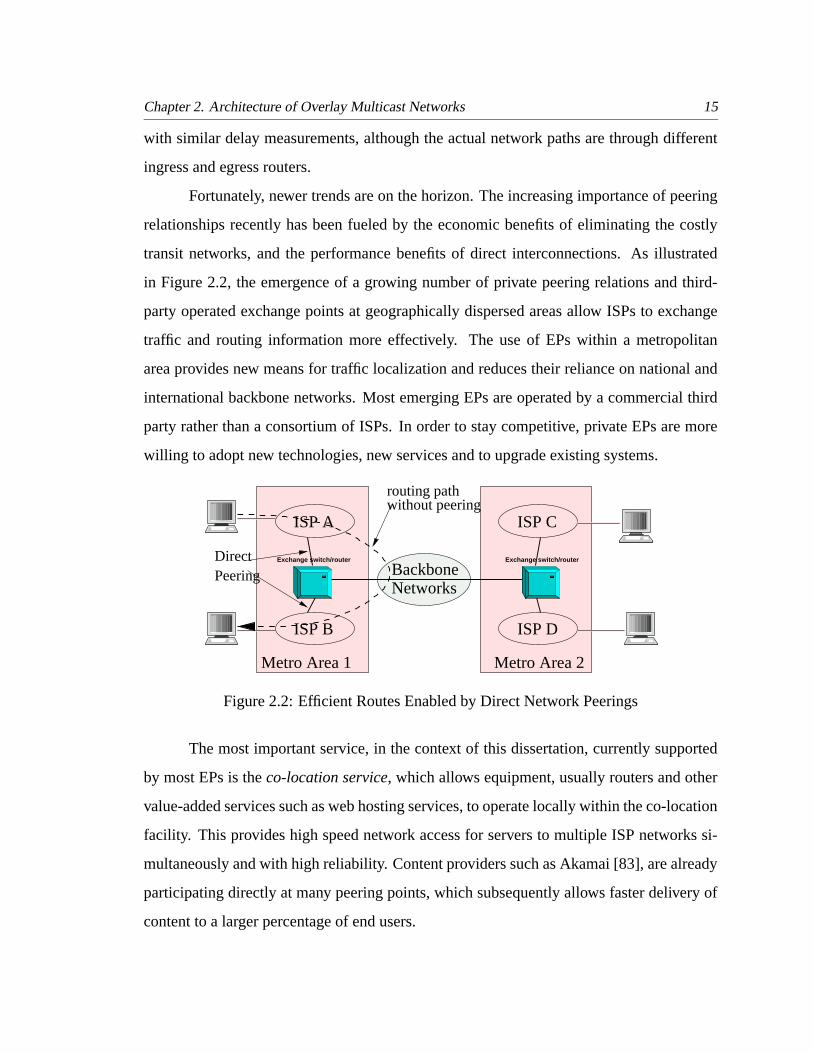
Fortunately, newer trends are on the horizon. The increasing importance of peering
relationships recently has been fueled by the economic benefits of eliminating the costly
transit networks, and the performance benefits of direct interconnections. As illustrated
in Figure 2.2, the emergence of a growing number of private peering relations and third-
party operated exchange points at geographically dispersed areas allow ISPs to exchange
traffic and routing information more effectively. The use of EPs within a metropolitan
area provides new means for traffic localization and reduces their reliance on national and
international backbone networks. Most emerging EPs are operated by a commercial third
party rather than a consortium of ISPs. In order to stay competitive, private EPs are more
willing to adopt new technologies, new services and to upgrade existing systems.
BackboneNetworks
without peeringrouting path
Metro Area 2Metro Area 1
Direct Peering
ISP A
ISP B ISP D
ISP C
Exchange switch/routerExchange switch/router
Figure 2.2: Efficient Routes Enabled by Direct Network Peerings
The most important service, in the context of this dissertation, currently supported
by most EPs is the co-location service, which allows equipment, usually routers and other
value-added services such as web hosting services, to operate locally within the co-location
facility. This provides high speed network access for servers to multiple ISP networks si-
multaneously and with high reliability. Content providers such as Akamai [83], are already
participating directly at many peering points, which subsequently allows faster delivery of
content to a larger percentage of end users.

Chapter 2. Architecture of Overlay Multicast Networks 16
The co-location service trends provide a foundation for the overlay network model.
The overlay service nodes, when co-located at EPs, can connect directly with end users of
different ISPs, overcoming the bottleneck of network interconnections. As the tier one ISPs
are likely to have presences at the EPs, the overlay service provider can select one of them
as its backbone network provider and route the aggregated local traffic directly to other
locations. As backbone networks have plenty of bandwidth capacity, an overlay service
provider can setup service level agreements with the backbone provider and be assured of
the path quality through the backbone. Therefore, the availability of broadband network
access from end users, the prevalence of network peering and exchanges, and the large
availability of backbone bandwidth give rise to opportunities for the overlay service model
for many next generation multicast applications.
2.2 Overview of Overlay Multicast Networks
We recall that an overlay network is a collection of data tunnels connecting network edge
routers or access routers, supporting the same processing functions. With the notion of
co-location services, the definition of network edges can be expanded to include servers
deployed within co-location facilities. The choice of providing network services by imple-
menting additional functions directly on the edge router platforms or by re-directing data
flows to the co-located servers depends on the type of services and the processing require-
ment for these services. For example, services such as DiffServ [6] and network security
can be implemented as processing functions on the access router platforms that apply to all
flows but require only small amounts of additional state; while services such as content dis-
tribution or network storage are more likely to use processing servers, since these services
only apply to a fraction of flows but require more managed resources. For the purpose of
this dissertation, we will not distinguish between these two alternatives but refer to them as
overlay networks in general.
Figure 2.3 illustrates a multicast service architecture using overlay networks. An
overlay multicast network provides services through a set of distributed Multicast Service

Chapter 2. Architecture of Overlay Multicast Networks 17
Nodes (MSN), which communicate with hosts and with each other using standard unicast
mechanisms. The MSNs act as proxies that forward and replicate data packets on behalf
of the senders. The data paths among MSNs within a session form a virtual multicast
tree, where each tree branch is a unicast connection. The association between a client and
its delegated MSN is decided by their relative locations, i.e. the MSN within the smallest
network distance of a client is selected as its proxy. We refer to this generic advanced
multicast model as AMcast.
ISP A
Internet
Content Server
End Users
End Users
End UsersMSN
ISP B
ISP C
multi-way conferencing
Figure 2.3: Overview of AMcast Architecture
Although the underlying data transmissions are over unicast connections, the AM-
cast network still supports the two advantages of multicast over unicast: a) it reduces the
transmission overhead on the senders; and b) it reduces the overhead on the network and the
time taken for all destinations to receive the data. The first advantage is clear since a sender
only needs to transmit one packet to its designated MSN instead of one copy to each group
member. The second advantage has been shown in several previous works [10, 13, 58, 91]
through simulations over various network topologies and a wide range of different multicast
trees.3
3To be more precise, all of these work study the problem under the condition that the MSNs are themselvesa subset of group members and vary with the groups; in [10], the network overhead is only measured onthe links among MSNs. Nevertheless, we will show that by placing the MSNs at strategic locations, thetransmission cost from group members to MSNs only adds a constant to the total cost, which validates theclaim.

Chapter 2. Architecture of Overlay Multicast Networks 18
We briefly describe the service model provided in AMcast and show how it over-
comes most of the issues existing in the IP multicast model.
Client and Session Identifications
Multicast address allocation has been a major source of inconvenience in the IP multicast
model due to the lack of scalable mechanisms to allocate a globally unique address in a
limited address space. The AMcast model solves this by identifying a session as a pair of
<host MSN, session id>, where the host MSN is the IP address of the MSN where
the session is initialized and session id is a locally unique number to the host MSN. Since
each MSN has a unique IP address, the session identifier is globally unique. The client
identifier is a similar pair: <MSN, client id>, where MSN is the proxy MSN for the
client. This is in spirit similar to the address allocation scheme in the EXPRESS [37] and
SSM [36] model.
Session Initialization
An AMcast session owner is typically the session initializer or the content provider. A
session owner has the right to specify the membership of the session. An AMcast session
can be established as a pre-established channel or on demand. A pre-established chan-
nel is suitable for Content Distribution Network (CDN) applications where the customers
subscribe to content channels through which data can be downloaded or pre-casted. The
session ID in this case can be embedded in the application which automatically downloads
the content once activated. On the other hand, a conferencing application can start the ses-
sion in an on-demand mode. The session owner obtains a session ID from its proxy MSN
and announces it through off-line methods such as email or web pages.
Data Forwarding
For each session that an MSN is a member of, it knows all other MSNs in the session and
all local clients in the session. The host MSN is responsible for computing the multicast

Chapter 2. Architecture of Overlay Multicast Networks 19
tree for the session and distributes the routing information to individual MSNs. A session
routing entry at an MSN points to its neighboring MSNs in the tree, as well as a local entry
pointing to its local clients in the session; these client entries are added or removed via
direct requests from the clients and are not propagated to other MSNs4. When receiving
data, an MSN forwards the data to all neighbors except where the packet is received from.
Additionally, it forwards packets to its local clients.
Access Control
An MSN does not have knowledge of all the existing sessions. When a session is requested,
the associated host MSN can be inferred from the requested session ID, and is consulted
to admit the new client. For conferencing applications, such consultation happens on the
fly by message exchanges between the proxy MSN of the new client to the host MSN
or directly to the session owner; and if admitted, the new client is added to the session
member list at it proxy MSN. For CDN applications and pre-established channels, the
session member list can be specified a priori and the MSN only needs to consult its local
database for client admission.
If the MSN does not participate in the session at the time of the client request, the
host MSN directs it to connect to an existing node in the tree; otherwise if the MSN is
already a member of the session, it only needs to activate its connection to the client. Such
localized control reduces the overhead for dynamic client joins and leaves.
Traffic Control
An MSN implements queue management on its outgoing interfaces for each session. A
buffer overflow at an outgoing interface indicates the session is sending more traffic than
the receivers’ capacity. This could indicate that either the sources are sending data too fast,
or some receivers (downstream of this interface) are too slow for the rest of the session.
To avoid performance penalties, sessions are forced to implement application-level rate4When access control is used, the client requests may be forwarded to the host MSN or the session owner
for admission. See discussion on access control.
Chapter 2. Architecture of Overlay Multicast Networks 20
control mechanisms. References [68, 87] propose ways for controlling rates for multicast
applications. The queuing mechanisms are ultimately necessary to prevent malicious or
irresponsible sources from abusing the overlay services. Fair queuing mechanisms such as
Deficit Round Robin [79] can achieve fair bandwidth usage with very little extra state at the
MSNs.
For some CDN channels, it may be desirable to have an open channel, which every-
body is allowed to join. Such an open channel is subject to source control: except when
specified by the session owner, a member can only receive but not send data to the channel.
The source control mechanism prevents possible DDOS attacks.
2.3 Benefits of Overlay Multicast Networks
The most prominent benefit of AMcast is that it does not require any network support ex-
cept the network unicast capabilities. This allows service diversities, as well as accelerated
service deployment. As a service infrastructure, service providers also have a greater level
of flexibility to provision and engineer their own networks to best meet the requirements of
the target applications, which is a goal that cannot be easily accomplished when multicast
is implemented as a network level mechanism due to the heterogeneity of the networks
and the heterogeneity of the applications. To demonstrate these latter benefits, we compare
AMcast with the IP multicast backbone – Mbone [21], which reflects the original attempt
by the network community to implement multicast in the wide area networks.
Mbone is an IP level overlay network in which packets belonging to a multicast
stream carry a class D IP address. Since the support of IP multicast is not turned on at
all routers, those routers that support the multicast delivery set up direct routes to each
other using the DVMRP routing algorithm. The IP packet forwarding engine examines
each packet’s destination address to see if it is a multicast packet or not. If it is, the packet
is duplicated and forwarded to the appropriate interfaces set up by the multicast routing
daemon. The Mbone has demonstrated the following problems, which AMcast is able to
overcome:

Chapter 2. Architecture of Overlay Multicast Networks 21
Routing Scalability:
By scalability of a multicast scheme, we mean the amount of routing information required
to deliver a multicast packet. In the case of Mbone, every router keeps routing information
for each multicast group and for each source of the group. This large amount of information
is not sustainable as the number of groups grows and especially the number of multi-source
applications, such as conferencing, grows. To make matters worse, the IP multicast address
space is flat and contains neither topological or geographical meaning; therefore the meth-
ods of address aggregation and hierarchical routing which make unicast able to sustain the
growth of the network, cannot be applied.
In AMcast, on the other hand, an MSN only needs to maintain routing information
for the groups that it is a member of. No source information is necessary since the AMcast
tree is a shared tree. An MSN does maintain information for all the end users that it serves
as a proxy, however, updates to this user information remains local to each MSN, and does
not incur global message exchanges.
Topology Manageability:
The Mbone has no central management, instead, it relies on individual sites that are mul-
ticast capable to build tunnels to connect to each other. The choice of a tunnel is largely
based on availability. Overall, the Mbone topology is not optimized and grows randomly.
It is also prone to mis-configurations and consequently to service disruptions.
The AMcast network, on the other hand, explicitly manages its topology: the MSN
locations are selected so as to best serve all user demands. They are direct peers with the
backbone routers, allowing optimization of overlay routes with respect to the underlying
network topology. The access links from MSNs to the routers are dimensioned in pro-
portion to traffic demand and the routing algorithm implements load balancing to avoid
congestion on any of these access links or overloading any of the MSNs. In short, the
AMcast network is a service network that can be routinely managed and upgraded, and
consequently, it can provide more reliable service to users.

Chapter 2. Architecture of Overlay Multicast Networks 22
Deployment Complexity:
The consequence of trying to implement multicast as a network primitive requires routers
to support native mode multicast; this is hard because the IP multicast model is very open
and uncontrolled, and the IP multicast routing protocols regard the network as a large, flat
topology rather than one that is hierarchical and consists of multiple independent adminis-
trative domains. To this date, there is no truly inter-domain multicast routing protocol that
is mature enough to be deployed.
The AMcast model takes a very different approach: it offers multicast as a service
level infrastructure and requires no support from the underlying network other than the
unicast capability. The deployment of an AMcast network is therefore solely decided by
the service provider, driven by the application demands.
2.4 Cost of Overlay Multicast Networks
In this section, we consider how overlay multicast compares to native multicast, in terms
of its efficiency in the use of the underlying networks. Since packets in an overlay network
cannot be replicated at the exact branching points in the physical network, there are du-
plicate packets transmitted on some of the links. Figure 2.4 shows an example of how an
overlay multicast session can use more than the ideal amount of network resources.
The network topology, in this example, consists of three MSN nodes (filled circles)
and three router nodes on a grid map. The MSN nodes are routers with co-located MSNs.
For simplicity, we assume all nodes have directly attached users of the multicast session,
so every node is a member of the multicast group. Figure 2.4(b) shows an optimal cost
network multicast tree, which is also a minimum spanning tree where tree cost is propor-
tional to the inter-node distance. Figure 2.4(c) shows an AMcast virtual multicast tree. The
connection between routers to the MSNs assumes all users and consequently their attached
routers are assigned to their closest MSNs. Since each tree branch is a unicast connec-
tion, each of them takes the network shortest path. Figure 2.4(d) shows the mapping of the

Chapter 2. Architecture of Overlay Multicast Networks 23
A B C
D
GF
(a) Network topology: the filled nodes indicate theco-location with routers where MSNs are available;the unfilled nodes indicate where end users sub-scribing to the multicast group are attached.
A B C
D
GF
(b) An optimal cost multicast tree at the networklevel: a minimum spanning tree.
A B C
D
GF
(c) An AMcast multicast overlay tree including treebranches between MSNs as well as tree leaves froman MSN to its end users, assuming end users arealways assigned to the closest MSN.
C
GF
A
D
B
(d) The mapping of the AMcast overlay tree to theactual network path for each tree branch. The ar-rows indicate the direction of the packet flow if Ais a data source.
Figure 2.4: An Example of the Mapping between Network Topology and AMcast VirtualTree Topology
overlay multicast tree to the actual data flow path. Clearly, the overlay multicast tree is sub-
optimal in two aspects: (a) the total cost of the tree is higher than the minimum spanning
tree since the unicast paths overlap on some of the edges; (b) the overlapping of network
paths causes additional load on the overlapped edges, which may unnecessarily result in
network congestion. Contrarily, any edge in a network-level multicast tree carries exactly
one copy of each packet.
So does overlay multicast make excessive use of network resources? In the rest of
this section, we answer this question in the negative by performing a systematic evaluation

Chapter 2. Architecture of Overlay Multicast Networks 24
on a range of overlay multicast trees and investigate their influences on the underlying net-
work topology and on the application performance. The comparison of the characteristics
of overlay multicast trees is made against other network level multicast trees; we do not
compare directly with unicast schemes as the latter become exorbitantly expensive with
increased size of multicast sessions, making any multicast scheme attractive.
As we will show in Chapter 3, the creation of overlay multicast trees poses NP-hard
problems if we try to optimize the MSN resource usage and the network delay simultane-
ously. The resulting trees therefore do not guarantee the characteristics of the trees that
affect the performance of the underlying network and the performance perceived by the
applications. Without going through the details of the routing algorithms, we will use the
minimum spanning overlay tree as an example to evaluate the overlay tree model for the
time being, and we will revisit these evaluations on more specific overlay trees in Chapter 3.
We use two network level multicast trees for comparison, one optimized for tree
cost, the other optimized for end-to-end delay. Steiner tree – A Steiner tree is the optimal
multicast tree in terms of the total cost. Formally, the network Steiner problem is: given an
edge-weighted graph and a subset of vertices S, find a minimal tree spanning all vertices
in S. The Steiner tree problem is NP-complete [26]. We will use the MST heuristic [27] to
approximate the optimal Steiner tree. The MST heuristic has an approximation ratio of 2,
which is very close, but with much less complexity than the best known approximation ratio
of 11/6 given by Zelikovsky [90]. Shortest path tree – The shortest path tree is widely
used in IP multicast and in some of the application-level multicast routing algorithms [10,
13]. A shortest path tree is a rooted tree such that the distance between any vertices in the
tree to the root vertex is minimum; this is the best tree to minimize the network delay. Due
to asymmetric network paths, shortest path trees are source-rooted. In multicast sessions
with multiple sources, each of the sources transmits over a separate shortest path tree. In
many multicast applications, each session member is potentially a source, therefore, we
will use the average cost of all shortest path trees, rooted at individual members, as its tree
cost. These alternatives for implementing multicast are evaluated using three criteria:

Chapter 2. Architecture of Overlay Multicast Networks 25
Transmission Cost:
The transmission cost measures the average network cost of sending a packet from one
group member to the rest of the group. In the case of an overlay multicast tree, the trans-
mission cost includes the edge cost along the unicast paths from each multicast client to
its designated MSN and the path cost of the multicast tree among the participating MSNs.
This also includes the cost of multiple traversals on some of the network links. For network
level multicast trees, the transmission cost is the sum of costs for all edges in the tree.
Link Stress:
The stress of the link measures the number of duplicate packets on a single network link.
When an MSN follows unicast paths to forward packets to its users and to other MSNs, it
may receive and send data over the same network interface, causing duplicate packets on
links close to the MSN. The stress, therefore measures the additional load on a network link.
As we assume that MSNs co-locate with routers, the stress measures all but the duplicates
on links from MSNs to their directly peered routers, since these only incur cost to service
providers – the cost of obtaining more bandwidth capacity at the MSN access links. The
stress for any network level multicast tree is one.
Relative Delay Penalty:
The RDP measures the ratio of delay between a pair of members along the overlay tree and
the delay over their network shortest path. For an instance, in Figure 2.4(d), the shortest
path between node A and B is one hop distance away, however, when propagating along
the overlay multicast tree, a packet will take three hops from A→D→A→B, resulting in a
RDP of three. The RDP measurements, therefore, show the relative detour of each packet
when sent over a multicast tree. A shortest path tree has an RDP of one, and a Steiner tree
has an RDP greater than one but typically less than that of the overlay tree.

Chapter 2. Architecture of Overlay Multicast Networks 26
Session Delay Penalty:
The SDP is an alternative (and arguably more relevant) measure of application delay per-
formance. The SDP is the ratio of the maximum delay on the tree path between two nodes
in a multicast session to the maximum network delay between any pair of nodes in the
session. This measures how much worse the worst tree path is to the worst intrinsic delay
among the nodes in the session. In our example, the maximum network delay among ses-
sion nodes is the path between C to G of length 5.25; the maximum delay on the tree path is
B to G where the sum of the underlying network paths (BCBADG) is 6.25 in length. This
results in an SDP of 1.19.
2.4.1 Evaluation Methodology
It is generally hard to construct a network topology that is representative to the current
Internet. Popular topology generators such as GT-ITM [89] assume certain network hier-
archies and generates random graph for each network layer. Recently the University of
Oregon Route Views Project [69] has provided many researchers the accessibility to part
of the global routing table exported from about 40 different Autonomous System domains,
and which constructs an AS-level network map.
Unfortunately, neither of them can model the geographical properties of the Internet.
As bandwidth becomes more abundant and network inter-connectivities become richer, the
cost and delay of the network are largely determined by geographical distances. For this
reason, we construct our network topology taking geographic considerations into account.
Specifically, both link delay and link cost are assumed to be proportional to geographic
distance.
Node Distribution
Figure 2.5 depicts the two topologies that we used in the simulation: one configuration in-
cludes 500 nodes randomly distributed over a disk space (the disk topology); and the other,
called the metro topology, contains backbone routers at each of the 50 largest metropolitan
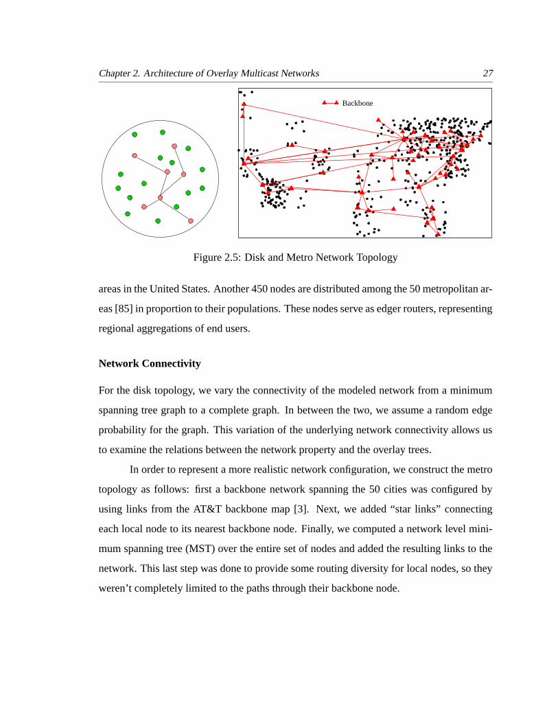
Chapter 2. Architecture of Overlay Multicast Networks 27
Backbone
Figure 2.5: Disk and Metro Network Topology
areas in the United States. Another 450 nodes are distributed among the 50 metropolitan ar-
eas [85] in proportion to their populations. These nodes serve as edger routers, representing
regional aggregations of end users.
Network Connectivity
For the disk topology, we vary the connectivity of the modeled network from a minimum
spanning tree graph to a complete graph. In between the two, we assume a random edge
probability for the graph. This variation of the underlying network connectivity allows us
to examine the relations between the network property and the overlay trees.
In order to represent a more realistic network configuration, we construct the metro
topology as follows: first a backbone network spanning the 50 cities was configured by
using links from the AT&T backbone map [3]. Next, we added “star links” connecting
each local node to its nearest backbone node. Finally, we computed a network level mini-
mum spanning tree (MST) over the entire set of nodes and added the resulting links to the
network. This last step was done to provide some routing diversity for local nodes, so they
weren’t completely limited to the paths through their backbone node.

Chapter 2. Architecture of Overlay Multicast Networks 28
Client and Server Placement
Given a network configuration, we want to place a specified number of servers in the net-
work so as to minimize the connection cost from all possible clients to servers. This maps to
the k-median problem, which finds k server locations such that the total cost of connecting
each client to its nearest server is minimized.
The k-median problem, however, is NP-complete [16]. In [34], Hochbaum intro-
duced a greedy heuristic algorithm that gives an O(log n) approximation ratio, where n is
the number of nodes in the graph. The O(log n) ratio is by far the best known approxima-
tion ratio for the k-median problem. We will use this greedy heuristic when placing servers
in the random graph. Although the k-median approach gives the best placement of servers,
a realistic configuration in the metro topology is likely to limit the location of the servers
to coincide with large cities due to the availability of local resources. We therefore only
allow the placement of a server in one of the 50 largest cities with respect to the objective
of minimizing the total cost from clients to servers.
In each simulation, we randomly select a number of multicast clients among all
nodes. A client then is assigned to its closest server and only those servers that have at-
tached clients will participate in the multicast session.
2.4.2 Comparisons with Network Multicast Trees
Disk Configuration:
Figure 2.6 shows the comparison of the minimum spanning overlay multicast tree with
network multicast trees on the disk configuration. Unless otherwise mentioned, the default
parameters used in these simulations are: each session includes 100 randomly selected
nodes, the number of MSNs placed is 50, the edge probability for the disk topology p =
0.005, and the disk radius is one unit. In Figure 2.6(a) , the cost of the trees is measured as
the total distance of sending one packet to the multicast session. Figure 2.6(a) shows the
cost trend of the three multicast trees with varied network connectivity from a sparse graph

Chapter 2. Architecture of Overlay Multicast Networks 29
to a complete graph; the x-axis shows the varied edge probability of the underlying random
graph. All plots are an average over 10 simulation runs.
0.001 0.01 0.1 1Edge Probability
0
20
40
60
80
100
Avg
. Dis
tanc
e / P
acke
t Tra
vel
Approx. Steiner TreeShortest Path TreeMinimum Spanning Overlay (S20)Minimum Spanning Overlay (S50)
50 100 150 200Session Size
10
20
30
40
50
60
Avg
. Dis
tanc
e / P
acke
t Tra
vel
Shortest Path Tree
Minimum Spanning Overlay (S20)
Minimum Spnanning Overlay (S50)
Approx. Steiner Tree
(a) Overlay Tree Cost
0.001 0.01 0.1 1Edge Probability
0
2
4
6
8
Dep
licat
e P
acke
ts P
er L
ink
20 Servers50 Servers
Max Stress
Avg. Stress
50 100 150 200Session Size
0
2
4
6
8
10
12D
eplic
ate
Pac
kets
Per
Lin
k
20 Servers50 Servers
Avg. Stress
Max Stress
(b) Link Stress
Both the cost of the approximate Steiner tree and the overlay tree decreases with the
increase of network connectivity, indicating a better utilization of the network resources.
The shortest path tree, on the other hand, sees an increase of its cost with a better connected
network. This is because the shortest path tree always concentrates on minimizing the
delay, and with the increase of available edges, each source is more likely to use a different
path to reach each destination. In particular, if the underlying network assumes a complete
graph, a shortest path tree is equivalent to the source using unicast to reach each destination.
As most IP multicast protocols continue to use the shortest path tree approach and as the
backbone network becomes more richly connected, the inefficiency of the shortest path tree

Chapter 2. Architecture of Overlay Multicast Networks 30
0.001 0.01 0.1 1Edge Probability
1
1.5
2
2.5
3
3.5
4
4.5
5
Rel
ativ
e D
elay
Pen
alty
(R
DP
)
Approx. Steiner TreeMinimum Spanning Overlay
90% RDP
Avg. RDP
50 100 150 200Session Size
1
2
3
4
5
Rel
ativ
e D
elay
Pen
alty
(R
DP
)
Minimum Spanning OverlayApprox. Steiner Tree
90% RDP
Avg. RDP
(c) Relative Delay Penalty
0.001 0.01 0.1 1Edge Probability
1
2
3
4
Tre
e D
iam
eter
/ M
ax S
essi
on D
elay
S50
Approx. Steiner Tree
Minimum Spanning Overlay
S20
50 100 150 200Session Size
1
2
3
4
Tre
e D
iam
eter
/ M
ax S
essi
on D
elay
S50
Approx. Steiner Tree
Minimum Spanning Overlay
S20
(d) Session Delay Penalty
Figure 2.6: Tree Comparison on Disk Configuration
becomes worse. Figure 2.6(a) shows that with the increase of session size, the cost of the
shortest path trees also remains higher than the overlay tree.
Figure 2.6(b) shows the stress measurement on the network links with the overlay
multicast tree. The network multicast trees always have a stress of one. We only measure
the stress at the interface links of the MSNs, since these are the places where most duplicate
packets occur. The average stress would be lower if we average the number of duplicate
packets over all network links used in a session. The duplicate packets occur when an MSN
sends the packet over the same interface where the packet is received from. On average,
this occurs once per interface as the average stress is measured at around two. There are

Chapter 2. Architecture of Overlay Multicast Networks 31
some links, however, that may sustain a higher stress, shown by the maximum stress. This
is further exacerbated if the number of MSNs in the network is small.
The relative delay penalty in Figure 2.6(c) shows the overlay multicast tree performs
slightly worse than the approximate Steiner tree. With a network of multiple paths, there
is no single tree that can minimize the delay between all pairs of members. The shortest
path trees achieve an RDP of one since it utilizes one tree for each source. The RDP for
the overlay multicast tree has an average of 2 to 2.5 and a 90 percentile of 3.5 to 4.5. We
observe that the large RDP values are more likely to occur between clients having small
network delay; this makes the denominator smaller, yet the absolute maximum end-to-end
delay along the overlay multicast tree is bounded at 6 unit of distance.
Figure 2.6(d) shows the session delay penalty with varied network connectivities
and session sizes. The curves for the overlay spanning tree and for the approximate Steiner
tree are quite close to each other, with the overlay tree outperforming slightly the approxi-
mate Steiner tree. The case when there are 20 MSNs (labeled as S20) in the overlay network
outperforms the case of having 50 MSNs (S50), since the latter has more MSNs involved
in a session, leading to longer tree paths. However, having more available MSNs in the
network generally gives better performance as indicated by the cost and the stress metrics.
Metro Configuration:
Figure 2.7 shows a similar set of tree comparisons performed on the metro configuration.
Here, we show the transmission cost as the relative cost ratio over the approximate Steiner
tree cost.
The metro configuration differs from the disk configuration in that it attempts to
model the network with a two-level hierarchy: the top level is the backbone network con-
necting 50 largest cities in US and the bottom level consists of regional routers directly
connecting to the backbone. This implies that the overlay multicast tree is likely to align
with the backbone network, with each tree branch corresponding to one or more backbone
links. This topology alignment should help the overlay multicast tree to reduce the stress

Chapter 2. Architecture of Overlay Multicast Networks 32
and the RDP. Figure 2.7(c) and 2.7(d) shows that, as compared with the disk configuration,
both measurements reduce significantly.
Figure 2.7(a) shows the relative tree cost with varied session size for 20 and 50
MSNs, as well as the relative cost of the shortest path tree. While the overlay multicast
tree with 50 MSNs again outperforms the shortest path tree, it shows that both overlay
multicast trees have an increased cost with the growth of the session size, while the shortest
path tree cost holds constant. Dissecting the overlay multicast tree composition, we find
that the increase of cost can be mainly attributed to the point-to-point connection cost from
clients to the MSNs. Recall that in the metro configuration, the paths from regional routers
to the backbone consist of links that form a star and links that form an MST. While the
shortest path tree and the Steiner tree are able to aggregate the paths from regional routers
to the backbone by using the MST links, the overlay multicast tree always selects the star
links. With larger session size, this part of the connection cost dominates the total overlay
multicast tree cost. Figure 2.7(b) shows this effect further. With larger numbers of MSNs,
MSNs are placed closer to clients, reducing the overall overlay multicast tree cost. On
the other hand, with smaller numbers of MSNs, although the tree cost among the MSNs
reduces, the overall cost becomes higher.
We observe in Figure 2.7(c), that the maximum stress holds constant at 2 with 50
MSN. This is clearly a benefit of aligning the overlay topology with the network topology
so that the backbone links are better utilized with fewer duplicated packets. Figure 2.7(d)
shows that this alignment also helps the overlay multicast tree to achieve better RDP per-
formance than the approximate Steiner tree.
Figure 2.7(e) shows the session delay penalty for the minimum spanning overlay
tree with 20 and 50 MSNs, compared with the approximate Steiner tree. All curves are quite
close to each other. The crossover of the two curves for the 20 and 50 MSNs is because a
session node always selects the closest MSN as its proxy, so more MSNs are involved in a
session if there are more of them available in the network. For smaller sessions, the larger
number of MSNs results in longer tree paths; while for larger sessions, this is compensated
by the smaller distances from the clients to the MSNs.

Chapter 2. Architecture of Overlay Multicast Networks 33
50 100 150 200Session Size
1
1.5
2
2.5C
ost R
atio
Ove
r S
tein
er T
ree
Shortest Path TreeMinimum Spanning Overlay (s20)Minimum Spanning Overlay (s50)
(a) Relative tree cost with varied session size.
10 20 30 40 50Number of Servers
1.2
1.4
1.6
1.8
2
2.2
Cos
t Rat
io O
ver
Ste
iner
Tre
e
Shortest Path TreeMinimu Spanning Overlay
(b) Relative tree cost with varied number of MSNs.
50 100 150 200Session Size
1
2
3
4
5
6
Dep
licat
e P
acke
ts P
er L
ink 20 Servers
50 Servers
Avg. Stress
Max Stress
(c) Link Stress
50 100 150 200Session Size
1
1.5
2
2.5
Rel
ativ
e D
elay
Pen
alty
(R
DP
)
Minimum Spanning OverlayApprox. Steiner Tree
90% RDP
Avg. RDP
(d) Relative Delay Penalty
50 100 150 200Session Size
1
1.5
2
2.5
Tre
e D
iam
eter
/ M
ax S
essi
on D
elay
Approx. Steiner Tree
Minimum Spanning Overlay
S20
S50
(e) Session Delay Penalty
Figure 2.7: Tree Comparison on Metro Configuration

Chapter 2. Architecture of Overlay Multicast Networks 34
We conclude from these simulation results that it is possible to build overlay mul-
ticast trees to utilize network resources efficiently without straining the end-to-end delay
performance. Especially when the placement of the MSNs aligns well with the underlying
network topology, the overlay multicast tree not only incurs very little overhead on network
links, it also produces better delay performance than the optimal network level multicast
tree.
2.5 Overview of Design Issues
A service provider that wishes to deploy and operate an overlay network faces the problem
of constructing a least-cost network that will meet the needs of network users. Although
not an easy task, a service provider needs to make certain assumptions on the geographical
distribution of the potential clients and to estimate the probable traffic distributions. Then,
the service provider must answer the following questions in order to construct the network:
Where should the service nodes be deployed to best serve all the clients? How much ca-
pacity should be assigned to each service node? How should session requests be routed
to satisfy application requirements while ensuring that the collective routing choices result
in high network utilization? Each of these critical questions leads to a subproblem in the
overall network design problem. The coupling and interaction of these problems results in
a complex network design problem that typically cannot be solved exactly. For the most
part of this dissertation, we study each of the subproblems independently, and combine the
solutions to provide an overall solution to the overlay network design problem. Here, we
first outline the main issues in the design problem and explain how they differ from the
traditional network design problem.
Traffic Assumptions
The traffic assumptions that serve as the premise of any network design problem, merit
some considerations itself. Most of the previous work [43, 70] assumes a known matrix on
the inter-node traffic flows, and consequently focuses on the problem of how to best fit this

Chapter 2. Architecture of Overlay Multicast Networks 35
traffic into the network links and routing paths. By the Law of Large Numbers, it is fairly
safe to assume that the aggregation of traffic flows from a large population behaves in a pre-
dictable fashion, and the average point-to-point traffic demand therefore can be estimated
in advance. However, complications arise in the context of multi-point communications,
where the number of nodes involved with each flow varies. This makes it prohibitively ex-
pensive, if at all possible given the lack of evidence on the distribution of multicast session
sizes, to obtain the traffic matrix. With this reason, we are forced to use simulations to
generate and compute traffic load with statistical models on the more primitive parameters.
This gives an estimation of the traffic load at individual sites under a fixed total network
offered load and the computed load will then be used to determine the amount of bandwidth
necessary at the individual sites.
Topology Design
The topology design problem is to find the placement of network nodes – routers in the
conventional network context, and MSNs in the overlay network context, and to decide
how to connect these nodes with respect to some network reliability and link capacity
constraints. With overlay networks, the second part of the problem does not exist since
the connectivity among MSNs is a full-mesh with each connection a unicast path through
the physical networks. The topology design problem therefore concentrates on finding the
placement of the MSNs, given the geographical locations of network clients.
With the economy of scale, it may be worthwhile to argue that a single node with
extremely large capacity, directly servicing all potential clients, is the cheapest design with
respect to the total cost of acquiring the amount of capacity and the cost of maintaining
the data centers. Indeed, this is the strategy adopted by service giants like America On-
line (AOL) for servicing their 34 million dial-up customers [84]. However, such a model
is not suitable for next generation applications with their increased data rates and the re-
quirements for small response times. In the single node design, the response time between
two clients on the same coast of the US may amount to the time required to traverse the

Chapter 2. Architecture of Overlay Multicast Networks 36
continent. Thus, solving the placement problem in overlay networks has to take these new
application requirements into consideration.
Capacity Assignment
Once the network topology and the traffic load are known, we can assign link capacities for
a specific routing algorithm subject to a total fixed cost. In the case of overlay networks, this
refers to dimensioning the access link bandwidth at each MSN site, and interchangeably
we call it the link dimensioning process in the later chapters. The capacity assignment in
overlay networks differs fundamentally from the conventional approach, where the objec-
tive in the latter case is to minimize the average network delay by assigning link capacity in
relation to its traffic load [43]. Here, we want to reduce the likelihood of blocking a session
request by assigning more capacity to interface links that have higher traffic load. A ses-
sion request is blocked if one of the session nodes does not have enough bandwidth left to
support the session traffic originating, transiting and terminating at the node. In Chapter 4,
we show that the total capacity required in an overlay network is fixed for a given traffic
load and is so regardless of the routing strategies. Therefore, the hard part of the capacity
assignment problem is to find the appropriate distribution of this total amount to individual
nodes, and this distribution indeed depends entirely on the routing strategy in use.
Routing
The overlay multicast routing presents a few different aspects from traditional multicast
routing. Here, the primary resource for an overlay network is the access bandwidth to the
Internet at the MSNs’ interfaces. This interface bandwidth represents a major cost, and is
typically the resource that constraints the number of simultaneous multicast sessions that an
overlay network can support. Hence, the routing algorithms should seek to optimize its use.
Additionally, a multicast routing algorithm should ensure that it does not select routes that
contain excessively long paths, as such paths can lead to excessively long packet delays.
However, the objective of limiting delay can often conflict with the objective of optimizing
the access bandwidth usage. The problems of optimizing one parameter while treating the

Chapter 2. Architecture of Overlay Multicast Networks 37
other as a constraint are both NP-hard. In the next chapter, we introduce several heuristic
algorithms to approximate the constraint-based multicast routing problems.
2.6 Related Work
The overlay network has emerged as a powerful technology in the context of many applica-
tions such as content distribution networks (CDN) [10,15,83], distributed caching [59,63],
distributed service lookup [80], large scale network storage systems [45], fault-resilient net-
work routing [2], and many others. The primary function of the overlay network, however,
differs largely in these applications, and roughly can be categorized into two divisions: one
type of applications use the overlay network to provide persistent data flows between end
points, such as in AMcast and CDN applications; the other uses the overlay network as a
virtual storage, such as in caching, service lookup, and network storage systems. For the
latter type of applications, the routing in the overlay network is directed towards the loca-
tion of the requested data and the main issues in these applications are the management of
the data storage and to devise a scalable hashing scheme that maps the data to the service
node where it is stored.
The development of CDN services are largely from commercial vendors and thus
we do not know the methodologies they use to construct and provision their networks.
In [10], the author proposed Scattercast, an architecture for Internet broadcast distribution
as an infrastructure service. In Scattercast, strategically placed service agents dynami-
cally organize into a source-based distribution tree. Since most CDNs are single-source
applications, a source-based multicast tree fits them well, however, we have shown that
source-based multicast trees are not suitable for multi-source applications and that their
performance degrades with increases in network connectivity. Another focus of Scattercast
is the application transport layer that provides reliability and adapts to meet individual ap-
plication constraints. Although AMcast shares the same view point as Scattercast in that
they both view multicast implemented at a service layer than as a network primitive, the
focus of our work is more on the network design aspects of the overlay network while

Chapter 2. Architecture of Overlay Multicast Networks 38
theirs on the operational and functional issues of the overlay network. There are also many
application-level multicast schemes in the literature targeted at small multicast groups. We
defer their discussion to the related work section in chapter 6, where we introduce ALMI as
an application-level multicast scheme that compliments the AMcast services.
The X-Bone [82] is a system for the dynamic deployment and management of In-
ternet overlay networks. It uses a two-layer tunneling mechanism to create overlays with
automatic resource discovery and overlay configurations. The focus in [82] is the compo-
nents and features of the X-Bone architecture, yet if X-Bone is to be deployed as an open
platform service network, it faces the same network provisioning tasks as discussed in this
section.
The pioneering work on network design can be traced back to the early 60s and
70s by Kleinrock [43] and Schwartz [70], among several others. They investigated a much
broader design problem relating to the topological design, capacity allocation, routing and
flow control aspects of computer networks in a point-to-point communication environment.
In their network model, a traffic matrix is known in advance and the cost of the network
relates to the number of network links and link capacities. The goal is to find the least
cost network that minimizes the average message delay time or limits the maximum mes-
sage delay time between any pair of nodes. By applying queuing theory, they allocate the
optimal capacity to each link and compute the total network cost. The least cost network
among a set of varied network topology is then chosen. The fundamental difficulty in ap-
plying a similar principle to overlay multicast network design, is the complexity involved
in computing the related parameters in a multicast fashion. Particularly, there are nn−2
ways of establishing a multicast tree for a session size of n, making it impossible to com-
pute the traffic statistics on any of the paths. Moreover, the multicast traffic also depends
on parameters such as the size of the sessions, the set of nodes involved in each session,
etc, which are not present in a unicast environment. These added complexities ultimately
result in our simulation-based approach to solve the combined dimensioning and multicast
routing problem.

Chapter 2. Architecture of Overlay Multicast Networks 39
2.7 Summary
In this section, we introduced the overlay network model for providing multicast services
and argued that this overlay model is well-suited for the emerging trends in the Internet
architecture. We also investigated the feasibility of the overlay model by evaluating the
network cost associated with overlay multicast networks and comparing with network-
layer multicast schemes. Our results show that although overlay multicast is not as optimal
as the best possible network-layer scheme, it comes close in all of the evaluation param-
eters. Particularly, it appears that overlay multicast is more efficient in utilizing network
resources than the current IP multicast model. Convinced that overlay multicast is viable,
we proceeded to discuss the main issues related in designing and provisioning such a ser-
vice network from a service provider’s point of view. The next three chapters provide
detailed studies for each of these main issues.

40
Chapter 3
Multicast Routing in Overlay Networks
The problem of multicast routing in overlay networks is: given a set of MSN sites, each
with a specified amount of available interface bandwidth, how can we route multicast ses-
sions to make the best use of the available network resources, so as to accommodate the
maximum number of sessions, with acceptable application performance. Because overlay
multicast networks are built on top of a general Internet unicast infrastructure, rather than
point-to-point links, the problem of managing their resource usage is somewhat different
than in networks that have their own links, leading to differences in how they are best
configured and operated. The main differences are:
• Network reachability: The overlay network is a fully meshed network, as each node
is able to reach everybody else in the network via unicast connections. Therefore, un-
like in IP multicast where a path from one router to another is defined by its physical
connectivity, an n-node overlay multicast session could have nn−2 different spanning
trees [9], leading to a larger design space and more design complexity.
• Network cost: Historically, the cost of a network is determined largely by the sum
of the individual link costs. This is certainly true for network providers who have to
physically deploy the links or lease them from others. However, from an application
service provider’s point of view, the cost associated with provisioning an overlay
network is the total amount paid to gain access bandwidth at each server site to the
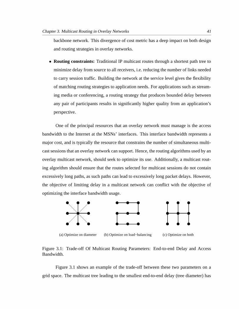
Chapter 3. Multicast Routing in Overlay Networks 41
backbone network. This divergence of cost metric has a deep impact on both design
and routing strategies in overlay networks.
• Routing constraints: Traditional IP multicast routes through a shortest path tree to
minimize delay from source to all receivers, i.e. reducing the number of links needed
to carry session traffic. Building the network at the service level gives the flexibility
of matching routing strategies to application needs. For applications such as stream-
ing media or conferencing, a routing strategy that produces bounded delay between
any pair of participants results in significantly higher quality from an application’s
perspective.
One of the principal resources that an overlay network must manage is the access
bandwidth to the Internet at the MSNs’ interfaces. This interface bandwidth represents a
major cost, and is typically the resource that constrains the number of simultaneous multi-
cast sessions that an overlay network can support. Hence, the routing algorithms used by an
overlay multicast network, should seek to optimize its use. Additionally, a multicast rout-
ing algorithm should ensure that the routes selected for multicast sessions do not contain
excessively long paths, as such paths can lead to excessively long packet delays. However,
the objective of limiting delay in a multicast network can conflict with the objective of
optimizing the interface bandwidth usage.
(a) Optimize on diameter (c) Optimize on both
(b) Optimize on load−balancing
Figure 3.1: Trade-off Of Multicast Routing Parameters: End-to-end Delay and AccessBandwidth.
Figure 3.1 shows an example of the trade-off between these two parameters on a
grid space. The multicast tree leading to the smallest end-to-end delay (tree diameter) has
Chapter 3. Multicast Routing in Overlay Networks 42
high traffic concentration on the center node; while the tree with most balanced access
bandwidth usage has an exceptionally long path. Thus, a multicast routing algorithm must
seek an appropriate balance between the optimization of these two parameters.
3.1 Problem Definitions
An overlay multicast network can be modeled as a complete graph since there exists a
unicast path between each pair of MSNs. For each multicast session, we create a shared
overlay multicast tree spanning all MSNs serving participants of a session, with each tree
edge corresponding to a unicast path in the underlying physical network. The degree of
an MSN node in the multicast tree represents the amount of access bandwidth in use to
support the multicast session and the total amount of available interface bandwidth at an
MSN imposes a constraint on the maximum degree of that node in the multicast tree. We
let dmax(v) denote this degree constraint at node v.
There are two natural formulations of the overlay multicast routing problem: the
first seeks to minimize the multicast tree diameter while respecting the degree constraints
at individual nodes; and the other optimizes the interface bandwidth usage to reduce the
likelihood of bottleneck nodes and constructs the tree satisfying an upper bound on the tree
diameter. We formalize the problems as follows.
Definition 3.1 Minimum diameter, degree-limited spanning tree problem (MDDL)
Given an undirected complete graph G = (V,E), a degree bound dmax(v) ∈ N for
each vertex v ∈ V and a cost c(e) ∈ Z+ for each edge e ∈ E; find a spanning tree T of G
of minimum diameter, subject to the constraint that dT (v) ≤ dmax(v) for all v ∈ T .
The second formulation of the overlay multicast routing problem seeks the “most
balanced” tree, that satisfies an upper bound on the tree diameter. To explain what is meant
by “most balanced”, we first define the residual degree at node v with respect to a tree T as
resT (v) = dmax(v)− dT (v), where dT (v) is the degree of v in T . To reduce the likelihood
of blocking a future multicast session request, we should choose trees that maximize the

Chapter 3. Multicast Routing in Overlay Networks 43
smallest residual degree. Since the sum of the degrees of all multicast trees is the same,
this strategy works to “balance” the residual degrees of different vertices. Any tree that
maximizes the smallest residual degree is a “most balanced” tree.
Definition 3.2 Limited diameter, residual-balanced spanning tree problem (LDRB )
Given an undirected complete graph G = (V,E), a degree bound dmax(v) for each
v ∈ V , a cost c(e) ∈ Z+ for each e ∈ E and a bound B ∈ Z+; find a spanning tree
T of G with diameter ≤ B that maximizes minv∈V resT (v), subject to the constraint that
dT (v) ≤ dmax(v), for all v ∈ V .
Both the MDDL and LDRB problems are NP-complete, since they contain the special
case in which every node has a degree of two, corresponding to the optimization and the
decision version of the Traveling Salesman Problem (TSP) [26], respectively.
Previous research has studied several related problems. In [32], Ho et al. proved that
in geometric space, there exists a minimum diameter spanning tree in which there are at
most two interior points (non-leaf nodes) and the optimal tree can be found in O(n3) time.
Hassin and Tamir established in [31], that for a general graph, a minimum diameter span-
ning tree problem is identical to the absolute 1-center problem introduced by Hakimi [29]
and as such, a solution can be found in O(mn + n2 log n), where n is the number of nodes
and m the number of edges. In [32] and [65] respectively, they prove that minimum diam-
eter, minimum spanning tree and minimum maximum degree, minimum spanning tree are
both NP-complete.
Although the special case of MDDL when all nodes have degree of two is hard to
solve, the problem might conceivably be less difficult when nodes have larger degree con-
straints. In the extreme case where all nodes have dmax(v) ≥ |V | − 1, there are no con-
straints on the nodes’ degree since the maximum possible degree for any node in a tree is
|V | − 1. In this case, the MDDL problem is polynomially solvable, since a minimum diam-
eter tree can be found by computing a shortest path tree rooted at each vertex and picking
the one with the smallest diameter. Next, we prove that even if all the degree constraints
are much larger than two, the problem remains NP-hard.

Chapter 3. Multicast Routing in Overlay Networks 44
We define MDDLk to be the MDDL problem restricted to instances for which dmax(v) =
k for all vertices in V .
Theorem 3.1 The decision version of MDDLk – finding a spanning tree with diameter
bound B and a degree constraint k for each vertex, is NP-complete, for integer k > 1.
Proof: Clearly, the problem is in NP, since we can verify in polynomial time if a candidate
solution satisfies both the diameter and degree constraints. Let G = (V,E) be the graph
of a TSP instance with a bound of B on path length. We transform an instance of TSP on
G to an instance of MDDLk on G′ = (V ′, E ′). We add k − 2 vertices u1, . . . , uk−2 to each
v ∈ V . We join each of these new vertices ui to v with an edge length of 0. Additional
edges of length B + 1 are added to G′ to make it a complete graph. There are a total of
|V |(k − 1) vertices in the MDDLk instance. Now, since any MDDLk solution must use the
k − 2 zero length edge to connect ui to v, and therefore, can only use two original edges at
each vertex. So the MDDLk instance in G′ has a spanning tree of diameter B if and only if
the TSP instance has a path of length B that includes all the vertices in G.
This result can be extended to handle values of k that are almost as large as the vertex
set of the graph. Given any TSP instance on m vertices, we can choose k = mr where r is
any fixed positive integer and apply the transformation used in the above proof to obtain an
MDDLk instance with k approximately equal to n1−1/(r+1), where n = m(k − 1) is the size
of the vertex set of the MDDLk instance. Since the MDDLk instance is only polynomially
larger than the original TSP instance, any algorithm to solve MDDLk optimally for such
large values of k, gives us a polynomial-time algorithm for TSP.
It is known that the TSP problem on a graph is MAX-SNP-hard even if edge
weights are restricted to 1 and 2 [55]. Since TSP is a special case for the MDDL problem,
the MDDL problem therefore cannot be approximated arbitrarily well unless P = NP . At
this time, we do not know the approximability of the MDDL problem in general. However,
we prove that there is no polynomial approximation scheme that can achieve a performance
ratio within any constant factor of the optimal, unless P = NP .

Chapter 3. Multicast Routing in Overlay Networks 45
Theorem 3.2 For the MDDLk problem, there is no polynomial approximation algorithm
that can achieve a performance ratio of C, for any fixed C.
Proof: We show that if there is such a polynomial approximation algorithm, then we can
solve the Hamiltonian path problem [26] in polynomial time. The proof contains a similar
construction to the one in Theorem 3.1. For any Hamiltonian path instance G = (V,E),
we construct an instance of MDDLk by filling out each node v with edges to the nodes
u1, . . . , ui, . . . , uk−2. These edges have zero weights. Let all edge weights be 1 in G′ and
assign weights C ∗ |V | to all other new edges. So we have edge weights
c(x, y) =
1 if x, y ∈ V
0 if x ∈ V, y /∈ V
C ∗ |V | otherwise
Then if G has a Hamiltonian path, the optimal solution to MDDLk has length |V |−1;
if we can find a solution to the MDDLk instance with diameter < C ∗ (|V | − 1), there must
be a Hamiltonian path in G.
In the next two sections, we first present two greedy heuristic algorithms for the
MDDL and LDRB problems; then we introduce a new algorithmic strategy for the LDRB
problem that takes a more direct approach to optimizing the MSN interface bandwidth.
Based on the second approach, we describe several specific tree-building techniques. These
algorithms are evaluated using simulation in chapter 4.
3.2 Routing Algorithms: Greedy Approach
In overlay multicast routing, we assume that there is a designated MSN (interchangeably a
host MSN) in each session which computes the multicast tree for the session. The desig-
nated MSN has full knowledge of other MSNs in the session, and computes the multicast
tree according to its current snapshot of the available bandwidth at these MSNs. State

Chapter 3. Multicast Routing in Overlay Networks 46
updates occur periodically via broadcasting among all MSNs. For the time being, we as-
sume that the designated MSN always has the most up-to-date information regarding other
MSNs, although in practice, it is likely that updates will occur less frequently than session
requests and that the routing performance may be reduced due to “stale” routing infor-
mation. We will examine this trade-off between the frequency of updates and the routing
performance in the next chapter.
The choice of the centralized route computation is to increase routing efficiency and
reduce message complexity by eliminating the many message exchanges required to co-
ordinate a distributed computation. We should point out that the centralized version does
not create a single point of failure or even a performance bottleneck, as each session may
select a different delegate to perform the tree computation. During periods of heavy net-
work load, we can expect there to be lots of session routing computations being performed
concurrently. This means that the overall computational load can be effectively distributed
by having different MSNs do the computation for different sessions. We believe that the
greater efficiency of this approach, relative to a distributed routing computation for each
session, will more than compensate for any inequalities in the load distribution that are
likely to arise in practice.
3.2.1 The Compact Tree Algorithm
The Compact Tree (CT) algorithm for the MDDL problem is a greedy algorithm, which like
Prim’s algorithm for Minimum Spanning Tree [14], builds a spanning tree incrementally.
For each vertex u in the partial spanning tree T constructed so far, let δ(u) denote the length
of the longest path from vertex u to any other node in T . For each vertex v that is not yet in
the partial tree T constructed so far, we maintain an edge λ(v) = {u, v} to a vertex u in the
tree; u is chosen to minimize δ(v) = c(λ(v))+δ(u). At each step, we select a vertex v with
the smallest value of δ(v) and add it and the edge λ(v) to the tree. Then, for each vertex
v, not yet in the tree, we update λ(v). This process is repeated for each vertex. Figure 3.2
illustrates an example and Figure 3.3 gives a detailed description.

Chapter 3. Multicast Routing in Overlay Networks 47
A B C
D
5
1 1
332
21
2
3
C
D
A B
5
1
3
21
2
3(a) A graph of 4 nodes, the numbers on thelines indicate the edge length and the num-bers around the nodes indicate the degreeconstraints.
(b) Start with node A as the root.λ(B) = {A, B}, δ(B) = 1λ(C) = {A, C}, δ(C) = 5λ(D) = {A, D}, δ(D) = 3Add node B to the tree.
C
D
A B
5
1
3
21
2
3
CA B
D
1
33
21
2
3
(c) Node B has reached its constraint, soλ(C) = {A, C}, δ(C) = 6λ(D) = {A, D}, δ(D) = 4Add node D to the tree.
(d) Update λ(C) = {C, D}, δ(C) = 7
A B
D
C1
33
21
2
3(e) The final tree. Note: If start with node D
as the root, we can construct a smaller diam-eter tree of length 6.
Figure 3.2: An Example of the Compact Tree Algorithm

Chapter 3. Multicast Routing in Overlay Networks 48
Input:G = (V, E)Edge cost c(u, v), for u, v ∈ V
Degree constraints dmax(v)Output: tree T
foreach r ∈ V doforeach v ∈ V do
δ(v) = c(r, v);λ(v) = {r, v};
T = (W = {r}, L = {}); D = dmax(r);while (W 6= V ) dolet u ∈ V − W be the vertex with smallest δ(u)and if |W | < |V | − 1, D + dmax(u) > 2;W = W
⋃
{u}; L = L⋃
{λ(u)}; D = D + dmax(u) − 2;foreach v ∈ W − {u} do
δ(v) = max{δ(v), distT (u, v)};foreach v ∈ V − W do
δ(v) = ∞;foreach q ∈ W doif degree(q) < dmax(q) and c(v, q) + δ(q) < δ(v) then
δ(v) = c(v, q) + δ(q);λ(v) = {v, q};
Figure 3.3: The CT Heuristic Algorithm for MDDL
The algorithm fails when it finishes with some vertices having δ(v) = ∞, meaning
that we cannot build a spanning tree with the specified set of degree constraints. There
are two cases where this can happen. One is that a session request may arrive at a set of
MSNs whose total available bandwidth (the sum of the degree constraints) is less than the
minimum required degree, 2∗(|V |−1), for a session spanning tree. In this case, the session
request is simply rejected. The other case is that during the progression of the algorithm, a
vertex with a degree constraint of one is added to the tree, when the sum of the spare degrees
of the tree vertices is also one. Such addition leaves the newly formed tree component with
zero spare degree and we cannot add any more nodes to the tree. To remedy this, we add a
count of the spare degrees of the tree component and defer the addition of a leaf node if it
reduces the count to zero.

Chapter 3. Multicast Routing in Overlay Networks 49
We have shown that there can be no polynomial algorithm that approximates the
MDDL problem to within a constant ratio. The CT algorithm, on the other hand, gives an
O(log n) approximation ratio with bounded edge weights. Let λCT and λ∗ denote the tree
diameter constructed by the greedy CT algorithm and an optimal solution, respectively.
And let d = min(dmax(u)) and D = max(dmax(u)).
Theorem 3.3 If the ratio of edge weights is bounded by ε ∈ Z+, and the degree constraints
satisfy 2 < d ≤ D < |V | − 1, then λCT < O(k)λ∗, where k = ε logd D.
Proof: Without loss of generality, let the smallest edge weight be 1 and the largest edge
weight ε. The optimal solution can do no better than λ∗ > 2 logD n. Now, let’s assume a
naıve algorithm A for constructing a spanning tree: at each step, A adds a new node with
the smallest degree constraint to an existing node in the tree whose degree constraint has
not been met. By keep adding nodes to an existing node as long as its degree constraint
allows, it results in a tree height of at most logd n. In the worst case, each selected edge has
weight of ε, so λA < 2ε(logd n). We observe that λCT ≤ λA. Because if all intermediate
nodes in tree T constructed by the CT algorithm are at their degree constraints, then λCT
cannot be worse than λA; If there is an intermediate node X in T that has not met its degree
constraint, then moving one of the leaf node that resides on the longest path in T to X
would increase the diameter of T . Therefore, λCT < kλ∗, where k = ε logd D.
3.2.2 The Balanced Compact Tree Algorithm
The Balanced Compact Tree (BCT) algorithm is a heuristic for the LDRB problem and
can be viewed as a generalization of the CT algorithm. Like the CT algorithm, it builds
the tree incrementally. However, at each step it first finds the M vertices that have the
smallest values of δ(v) and from this set, it selects a vertex v with λ(v) = {u, v}, that
maximizes the smaller of resT (u) and resT (v), where T is the current partial tree. The
parameter M may be varied to trade-off the goals of residual degree balancing and diameter
minimization. Specifically, when M = 1, it is equivalent to the CT algorithm; and when M
is equal to the number of vertices in the multicast session, BCT concentrates on balancing
Chapter 3. Multicast Routing in Overlay Networks 50
the residual degrees. Simulation studies have shown that fairly small values of M are
effective in achieving good balance, without violating the diameter bound.
In Chapter 4, we evaluate overlay multicast routing algorithms using a simulation in
which new multicast sessions are dynamically generated as a Poisson process. The primary
performance metric is the fraction of sessions that are rejected because no multicast route
can be found, either due to the failure to satisfy the diameter bound or due to the exhaustion
of interface bandwidth of at least one MSN. We also obtain a lower bound on the rejection
probability using a simulation in which a multicast session is rejected only if the MSN in-
terface bandwidth required by the session exceeds the total unused interface bandwidth at
all MSNs (including those not involved in the session). Results from the simulations show
that by distributing the load more evenly across servers, the BCT algorithm rejects substan-
tially fewer multicast sessions than the CT algorithm on the same network configuration.
At the mean time, there remains a significant gap between the achieved performance and
the potential suggested by the lower bound. While the bound was not expected to be tight,
the size of the gap suggested that there was room for improvement. In the next section,
we introduce a new strategy for overlay multicast routing that leads to an algorithm with
uniformly better performance.
3.3 Routing Algorithms: Balanced Degree Allocation
In the BCT algorithm, a new node is always attached to the tree at the point that yields
the smallest diameter in the resulting tree. Although the algorithm changes the sequence
of node selection by first selecting nodes with larger residual degrees, it does not guaran-
tee the use of these nodes as intermediate nodes in the tree, i.e. nodes with higher degree
fanout. This prevents the BCT algorithm from achieving the best-possible residual degree
balance. Naturally, we can think of an alternative strategy that approaches the problem in
a different way by first allocating the ideal degree of each node in the multicast session
and then constructing a multicast tree with respect to this pre-determined set of degree con-
straints. The ideal degree of each node is determined such that for a sequence of multicast

Chapter 3. Multicast Routing in Overlay Networks 51
session requests, the degree allocation scheme maximizes the number of sessions that can
be accepted.
Conceivably, we may consider an admission scheme in addition to the degree allo-
cation scheme that decides the set of requests to be accepted. An optimal algorithm for
routing a sequence of multicast session requests therefore, makes two decisions: first, it
decides if a session should be admitted or not; and second, if the session is admitted, it
allocates the appropriate degree for individual session nodes. The combined solution max-
imizes the total number of accepted sessions. However, the session admission problem
alone, regardless of the degree allocation scheme, is NP-complete. We define a session to
be admissible if upon its arrival, the nodes involved in the session satisfy the following two
conditions:
∑
v
dmax(v) ≥ 2(k − 1) and dmax(v) > 0 for all V
where k is the session size, or interchangeably session fanout. We now prove that even if
we know the sequence of session requests in advance, it is still hard to selectively accept
sessions in order to maximize the number of sessions that can be accepted.
Definition 3.3 Multicast session admission problem (MSA)
Given a set of network nodes V, n = |V |, each with a capacity ci ∈ N+, a set of
requests σ1 . . . σm, each consisting of k nodes in V , find the largest set of requests that can
be accepted.
Theorem 3.4 The MSA problem is NP-hard.
Proof: We reduce from the exact cover by 3-Sets(X3C) problem [26]. An instance of X3C
consists of a collection C of 3-element subsets (triples) of the base set X and has a solution
if and only if the given collection contains an exact cover of X that is a subset of C with
exactly |X|/3 triples whose union is X . We transform the X3C instance to an instance of
the MSA problem as follows: for each element define a network node. Next, we construct a
series of session requests with k = 4. Each of them includes the three nodes corresponding

Chapter 3. Multicast Routing in Overlay Networks 52
to a triple in the X3C instance plus an additional node Ai. We assign one unit of capacity to
each of the three nodes and capacity of 3 to the additional node; therefore the only way to
construct a multicast tree for a request is to create a star centered at Ai which then connects
to each of the three nodes. There are n + m network nodes in the MSA instance, where n
is the number of base set elements and m is the number of subsets. If the X3C instance has
an exact cover of size K, then K is the maximum number of sessions that can be accepted
since we have used all the available capacity at all nodes in V \A (where A is the union of
the additional nodes Ai). Conversely, if MSA can admit a maximum number of sessions
and since it can only select each node in V \A exactly once, we can decide if there is an
exact cover of X .
3.3.1 The Degree Allocation Problem
It is common in practice for a routing algorithm to accept a session as long as there are
available resources to support it, since future sessions and the possible gains from accepting
future sessions are unknown at the present. With this admission policy, we define a degree
allocation dA to be a function from the vertices of a multicast session to the positive integers
that satisfies two properties: (1)∑
v dA(v) = 2(k−1), where k is the number of participants
in the multicast session; and (2) there are at least two vertices u and v with dA(u) =
dA(v) = 1. A partial degree allocation is a similar function in which the first property is
replaced with∑
v dA(v) ≤ 2(k − 1). Now, define the residual capacity of a vertex with
respect to a partial degree allocation dA as resA(v) = dmax(v) − dA(v).
In the case of permanent sessions, where sessions have infinite durations, there can
be no degree allocation scheme that is more than 2(k − 1) times worse than the optimal.
We can make a simple argument for this: Let d∗(v) denote the degree of node v in a session
tree constructed by an optimal algorithm. The total capacity required for each session is
2(k−1) units for any algorithm. Therefore, if a session is rejected by the optimal algorithm
but accepted by a degree allocation algorithm A, the total amount of capacity in use that
could block future sessions, is 2(k − 1). On the other hand, if a session is accepted by

Chapter 3. Multicast Routing in Overlay Networks 53
both algorithms, consider only those nodes which have degree allocations greater than
their allocations by the optimal algorithm, the sum of degree differences of these nodes
is∑
i dA(v) − d∗(v) < k − 1. In the worst case, each one unit capacity in difference
can prevent one session accepted by the optimal algorithm from being accepted by the
algorithm A, therefore the worst case bound is 2(k − 1).
Although it seems hard to provide any worse case performance guarantee across
all possible request sequences, we still want to allocate nodes’ degrees in a way that re-
duces the likelihood of blocking future sessions. The Balanced Degree Allocation (BDA)
is a strategy that allocates degree more evenly among session nodes with respect to their
dmax(v), i.e it allocates a larger degree to a node with relatively large value of dmax(v) to
reduce the probability of having bottleneck nodes that could cause later session rejections.
In order to avoid bottleneck nodes, we need to maximize the smallest residual degree of
any node in the session. We can compute a degree allocation that maximizes the smallest
residual degree as follows.
• For each vertex v in the multicast session, initialize dA(v) to 1.
• While∑
v dA(v) < 2(k − 1) select a vertex v that maximizes resA(v) and increment
dA(v).
This procedure actually does more than maximize the smallest residual degree. It
produces the most balanced possible set of residual degrees, by seeking to “level” the resid-
ual capacities as much as possible, such that it minimizes, maxv(resA(v))−minv(resA(v)),
the difference between the largest and the smallest residual degree for all nodes in a session.
3.3.2 Algorithms Based On Balanced Degree Allocation
Given a degree allocation for a tree, we would like to construct a tree in which the vertices
have the assigned degrees and which satisfies the limit on the diameter. There is a general
procedure for generating a tree with a given degree allocation, which is described below.
The procedure builds a tree by selecting eligible pairs of vertices, and adding the
edge joining them to a set of edges F that, when complete, will define the tree. The spare

Chapter 3. Multicast Routing in Overlay Networks 54
degree of a vertex v, is its allocated degree dA(v) minus the number of edges in F that are
incident to vertex v. At any point in the algorithm, the edges in F define a set of connected
components. A pair of vertices {u, v} is an eligible pair if the following conditions are
satisfied.
• u, v are not in the same component;
• both u, v have spare degree ≥ 1;
• either, there are only two components remaining, or the sum of the spare degrees of
the vertices in the components containing u and v is greater than 2.
The last condition above is included to ensure that each newly formed component
has a spare degree of at least one, so that it can still be connected to other components in
later steps. Of course, this condition is not needed in the last step.
This process is guaranteed to produce a tree with the given degree allocation, and
all trees with the given degree allocation are possible outcomes of the process. We can get
different specific tree construction algorithms by providing different rules for selecting the
vertices u and v.
One simple and natural rule is to select the closest pair u and v. Call this the Closest
Pair (CP) algorithm. Since the CP algorithm does nothing to directly address the objective
of diameter minimization, it may not produce a tree that meets the diameter bound. An
alternative selection rule is to select the pair {u, v} that results in the smallest diameter
component in the collection of components constructed as the algorithm progresses. This
algorithm is referred to as the Compact Component (CC) algorithm.
One can also use a selection rule that builds a single tree incrementally. In this rule,
we consider all eligible pairs of vertices u and v, for which either u is in the tree built so
far, or v is in the tree, but not both. Among all such pairs, we pick the one that results in the
smallest diameter tree. This procedure is repeated for every choice of initial vertex, and the
smallest diameter tree is kept. This algorithm is the same as the CT algorithm described
before, but with the original input degree constraint dmax replaced with the much tighter
degree allocation dA.

Chapter 3. Multicast Routing in Overlay Networks 55
Any of the selection rules described will produce a tree with the desired degree
allocation. However, the resulting tree may not satisfy the bound on diameter. We can
reduce the diameter of the trees by using a less balanced degree allocation. To reduce
the diameter, we can increase the degree allocation of “central vertices” while decreas-
ing the degree allocation of “peripheral vertices”, where central and peripheral are de-
fined relative to vertex locations. A vertex u is more central than a vertex v if its radius
maxwc({u,w}) < maxwc({v, w}). Unfortunately, we have found that natural strategies
for adjusting degree allocations lead to only marginal improvement in the diameters of the
resulting trees. It appears difficult to find good degree allocations, independently of the tree
building process. We have found that a more productive approach is to use a “loose degree
allocation” and allow the tree-building process to construct a suitable tree satisfying the
degree limits imposed by the loose allocation. Loose degree allocations are derived from
the most balanced allocation by allowing small increases in the degrees of vertices.
By combining the tree building procedure, with a specific rule for selecting eligible
pairs and a procedure for “loosening” a degree allocation, we can define iterative algorithms
for the overlay multicast routing problem. We start with a balanced degree allocation and
build a tree using that allocation. If the resulting tree satisfies the diameter bound, we stop.
Otherwise we loosen the degree allocation and build a new tree. We continue this process
until we find a tree with small enough diameter, or until a decision is made to terminate the
process and give up.
The degree loosening procedure increases by 1, the degree allocation of up to b ver-
tices, where b is a parameter. The first application of the procedure adds 1 to the degree
allocation of the b most central vertices. If incrementing the degree allocation for a vertex
v would cause its degree allocation to exceed the degree bound for v, then v’s degree al-
location is left unchanged. The second round of the procedure adds 1 to the next b most
central vertices (again, so long as this would not cause their degree bounds to be exceeded).
Subsequent applications affect the degree bounds of successive groups of b vertices, and
the process wraps around to the most central vertices, after all vertices have been consid-
ered. The process can be stopped after some specified number of applications of the degree

Chapter 3. Multicast Routing in Overlay Networks 56
loosening procedure, or after all degree allocations have been increased to the smaller of
their degree bounds and k − 1 where k is the session fanout.
If we select eligible pairs for which the connecting edge has minimum cost, the re-
sulting algorithm is called Iterative Closest Pair (ICP) algorithm. If we select eligible pairs
so as to minimize the diameter of the resulting component, the algorithm is called Iterative
Compact Component (ICC) algorithm. In the Iterative Compact Tree (ICT) algorithm, we
select eligible pairs, with one vertex of each pair in a single tree being constructed, and the
other selected to minimize the tree diameter. This procedure is repeated for all possible
initial vertices.
An example execution of the ICT algorithm appears in Figure 3.4. For simplicity, we
used geographical distance as routing cost and a diameter bound of 8000 km. Initially, the
BDA output dictates the creation of a star topology with New York City as the center with
degree of 7; this exceeds the diameter bound. In the second round, the degree allocation of
three nodes with small radius, Las Vegas, Phoenix, Louisville, is loosened by 1; this results
in a tree satisfying the diameter bound. We observe that the actual degree allocation is still
close to the balanced degree allocation at most vertices.
Las Vegas (1)
New York City (7)
Washington D. C. (1)
Portland (1)
St. Petersburg (1)
Louisville (1)
Phoenix (1)
Miami (1)
(a) Longest Path: Portland → New York →Phoenix; Length = 9416.67 km
New York City (7)
Washington D. C. (1)
Portland (1)
St. Petersburg (1)
Louisville (2)
Phoenix (2)
Las Vegas (2)
Miami (1)
(b) Longest Path: Portland → Las Vegas →Phoenix → Louisville → New York → St. Pe-tersburg; Length = 7823.64 km
Figure 3.4: An Example of the ICT Algorithm with Degree Adjustment

Chapter 3. Multicast Routing in Overlay Networks 57
3.4 Cost of Overlay Trees Revisited
In section 2.4, we used the minimum spanning overlay multicast tree to study the cost and
other metrics of overlay trees, and showed that overlays are efficient in utilizing the network
resources as well as providing bounded end-to-end delay performance. By now, we have
established that the creation of the overlay multicast tree poses NP-hard problems when we
try to optimize on resource usage and application delay performance simultaneously. The
resulting trees therefore do not conform to a single characteristic; depending on resource
availability, they can range from a path to a star. In order to properly represent the variety,
we select the opposite ends of the spectrum and evaluate the cost of two types of overlay
trees: the minimum diameter overlay tree and the furthest chain overlay tree. The minimum
diameter overlay tree minimizes the longest simple path in the tree, and is the best to reduce
the end-to-end delay; The furthest chain overlay tree is a chain rooted at two nodes that are
furthest away from each other. A chain is the most load-balanced overlay tree, since each
node has a degree of either one or two. The computation of the furthest chain is equivalent
to the TSP problem and is NP-complete. We use the nearest insertion heuristic [33] to
approximate it. Each of these trees is ideal for one of the evaluation parameters but may be
very poor for the other. For instance, the minimum diameter tree is the best for reducing
network delay but typically results in a tree of high cost, and often contains nodes of high
fanout, resulting in high stress. Table 3.1 summarizes the trees and their corresponding
ideal and pathological scenarios. We use the same configuration as those described in
section 2.4.
Table 3.1: Summary of the Overlay Multicast TreesMetrics Ideal Scenario Pathological ScenarioTransmission cost Minimum spanning tree Minimum diameter treeLink Stress Furthest chain (with two furthest
MSNs as end points)Minimum diameter tree
Delay Penalty Minimum diameter tree Furthest chain

Chapter 3. Multicast Routing in Overlay Networks 58
3.4.1 Overlay Cost on Disk Configuration
0.001 0.01 0.1 1Edge Probability
0
20
40
60
80
100
Avg
. Dis
tanc
e / P
acke
t Tra
vel
Approx. Steiner TreeShortest Path TreeMinimum Spanning OverlayMinimum Diameter OverlayFurthest Chain
(a) Tree costs with varied underlying network con-nectivities. Session size is 100. The radius of thedisk is 1 distance unit. Number of MSNs is 50.
50 100 150 200Session Size
10
20
30
40
50
60
Avg
. Dis
tanc
e / P
acke
t Tra
vel
Approx. Steiner Tree
Minimum Diameter Overlay
Minimum Spanning Overlay
Shortest Path Tree
Furthest Chain Overlay
(b) Tree cost with varied multicast session size.Number of placed MSNs is 50, underlying networkedge probability p = 0.005.
50 100 150 200Session Size
0
5
10
15
20
25
Dep
licat
e P
acke
ts P
er L
ink
Minimum DiameterFurthest Chain
Average Stress
Maximum Stress
(c) Average and maximum link stress of the over-lay trees with varied number of clients. The edgeprobability is 0.05.
0.001 0.01 0.1 1Edge Probability
0
5
10
15
Rel
ativ
e D
elay
Pen
alty
(R
DP
)
Minimum Diameter TreeFurthest Chain
Max RDP
Avg. RDP
(d) Relative delay penalty with varied networkconnectivities and 100 clients.
Figure 3.5: Comparison of Overlay and Network Multicast Trees Over Disk Configuration
The disk topology models the network as a flat network. Figure 3.5(a) shows the
multicast tree costs with varying edge probabilities for the underlying network. In this
simulation setting, there are 100 clients. We observe that both the minimum spanning
overlay and the furthest chain remain relatively low cost through the entire graph. The cost

Chapter 3. Multicast Routing in Overlay Networks 59
of the minimum spanning tree is about 1.5 times that of the approximate Steiner tree. The
cost of the minimum diameter tree is slightly higher, but drops with the increase of network
connectivities to about 3.5 times of the approximate Steiner tree. The shortest path tree, on
the other hand, increases its cost with the increase of the network connectivity because it
always routes through the most direct links between a pair of members. In the extreme case
of a complete graph, i.e. when the edge probability equals 1, the shortest path tree forms a
star centered at the source; this is highly inefficient in terms of resource usage.
Any network level multicast tree has link stress of 1. The overlay multicast tree,
on the other hand, will have multiple packet traversals of the same link since the overlay
tree branching points do not align perfectly with the underlying network branching points.
Figure 3.5(c) shows the average and maximum link stress for the minimum diameter and
the furthest chain overlay trees with varied numbers of clients. On the average, the link
stress stays relatively low at around 2 for both trees. However, the maximum stress of the
minimum diameter overlay can be as high as over 20. This is because a minimum diameter
overlay can often result in a star topology. Consequently, links near the center of the star
have very high stress.
The shortest path trees have RDP of 1, however in any general topology, no single
tree can optimize on the delay between every pair of members due to the existence of
alternate routing paths. Figure 3.5(d) shows the average and maximum RDP between all
pairs of members. The minimum diameter overlay tree achieves an RDP ratio of 2 across
all network connectivities; this is better than the RDP of the approximate Steiner tree. The
furthest chain overlay has a relatively high average RDP of between 5.5 and 7.
3.4.2 Overlay Cost on Metro Configuration
The metro topology models the network as a two level hierarchy. The map obtained on the
AT&T backbone contains 68 backbone links interconnecting 50 backbone sites. We restrict
the placement of MSNs to be co-located with the backbone sites. Figure 3.6(a) shows the
relative tree cost over the Steiner tree cost with varied session sizes. Both the minimum

Chapter 3. Multicast Routing in Overlay Networks 60
spanning overlay and the furthest chain perform consistently better than the shortest path
tree, but the minimum diameter overlay tree has a relatively high cost. Since the cost of
connecting end users to the MSNs is the same for all overlay trees, the high cost of mini-
mum diameter overlay suggests that it tends to use more backbone links. Since backbone
links are more precious resources, the minimum diameter overlay tree is not very efficient
in this respect.
50 100 150 200Session Size
1
2
3
4
5
Cos
t Rat
io O
ver
Ste
iner
Tre
e
Shortest Path TreeMinimum Spanning OverlayMinimum Diameter OverlayFurthest Chain
(a) Relative tree cost with varied session size.Number of MSNs placed is 50.
10 20 30 40 50Number of Servers
1
2
3
4
Cos
t Rat
io O
ver
Ste
iner
Tre
e
Shortest Path TreeMinimum Spanning OverlayMinimum Diameter OverlayFurthest Chain
(b) Relative tree cost with varied number of serversand 100 clients.
50 100 150 200Session Size
0
5
10
15
20
Dep
licat
e P
acke
ts P
er L
ink
Minimum DiameterFurthest Chain
Max StressAvg. Stress
(c) Average and maximum link stress of the over-lay trees with varied number of clients.
50 100 150 200Session Size
1
2
3
4
5
Ave
rage
RD
P
Minimum Diameter Overlay
Furthest Chain
Approx. Steiner Tree
Minimum Spanning Overlay
(d) Relative delay penalty with varied number ofclients. The worst case RDP among all overlaymulticast trees is 7.5 of the furthest chain overlay.
Figure 3.6: Comparison of Overlay and Network Multicast Trees Over Metro Configuration

Chapter 3. Multicast Routing in Overlay Networks 61
Figure 3.6(b) shows the relative tree cost over the Steiner tree cost for a varied
number of MSNs with 100 clients. The average cost of shortest path trees holds constantly
at about 1.8 times the Steiner tree cost. For the minimum spanning overlay, the more the
number of MSNs, the lower the total transmission cost. Although increasing the number
of MSNs will increase the cost of the minimum spanning overlay among MSNs, it allows
MSNs to be placed closer to the clients which reduces the total cost of regional access links.
Again, both the minimum spanning overlay and the furthest chain outperform the shortest
path tree. On the other hand, the minimum diameter overlay performs rather poorly: its
cost goes up with the increase in MSNs. This is because the minimum diameter overlay
often creates a star topology which is not very efficient in aggregating flows and uses as
many direct paths as possible, hence the higher cost.
Figure 3.6(c) shows the link stress of the minimum diameter and the furthest chain
overlay on the metro topology. In this case, we only show the stress on the backbone links
since they are more expensive. Both of the trees have a low average stress of about 2.5,
which remains low with the increase in clients. The maximum link stress of the furthest
chain is also very small in this case, while the minimum diameter overlay has a higher
stress measurement. These patterns are consistent with those in the disk configuration.
0 2000 4000 6000 8000Physical Network Delay (km)
0
2000
4000
6000
8000
Ove
rlay
Net
wor
k D
elay
(km
)
Avg. RDP = 2.65
90% RDP = 5.63
y = 7500 kmlarge RDPs
Figure 3.7: Pairwise Delay Performance of Overlay Trees
Chapter 3. Multicast Routing in Overlay Networks 62
The RDP plot in Figure 3.6(d) shows that all three trees have relatively constant de-
lay performances. We observed that the large RDP values mostly occur between members
that have small network delay but relatively larger delay along the overlay tree. Figure 3.7
shows the delay for every pair of nodes in the session. The top left corner plot are pairs of
large RDPs. Since the largest RDPs (ratio of y value to x value) are for node pairs that are
close in the physical network, the true impact of this is much smaller than the RDP values
suggest. The absolute delay is bounded at 7500 km, which is reasonably good given that
the longest end-to-end delay in the metro configuration delay is a little over 6000 km.
We did not show a graph for the SDP measurement here, since the SDP value is
directly influenced by the diameter bound specified to the routing algorithms. Any trees
that fail to meet the diameter bound are rejected by the routing algorithm, so the average
SDP value is less than the ratio of the diameter bound against the maximum network delay.
The diversity of trees evaluated in this section bounds the worse case behavior of an
overlay tree as a result of our routing algorithms in all three metrics. From these measure-
ments, we conclude that with the exception of minimum diameter overlay, the overlay trees
are almost as efficient as the optimal network-level multicast schemes. With the use of the
BDA strategy, the chance is small to create minimum diameter trees for a large number
of sessions since BDA tends to even out the interface bandwidth usage at each MSN. The
RDP performance, on the other hand, is somewhat less encouraging. One particular con-
cern is that two locally close clients cannot take advantage of their proximity in the overlay
model. Although for most applications, it is not critical to have the smallest delay possible
as long as the maximum can be bounded, for applications that can take advantage of this
partial speedup within a group, it is conceivable to have some form of multicast gateway
services that bridge the native multicast in local networks to the overlay multicast session.
We will leave this as future work.

Chapter 3. Multicast Routing in Overlay Networks 63
3.5 Related Work
The existing IP multicast protocols: DVMRP [4], MOSPF [52], CBT [5], PIM [22] and
SSM [36], all create shortest path trees (SPT) for data dissemination. Both DVMRP and
MOSPF create a per-source based shortest path tree, CBT and PIM-SM create a shared
shortest path tree rooted at the “core” or the Rendezvous Point (RP),1 and SSM is a single-
source multicast protocol. The advantage of SPT is that it is easy to compute and can be
implemented in a distributed fashion efficiently. The main disadvantage of using per-source
SPT is its limited scalability with large numbers of sources and that it is not cost efficient
in a network with rich connectivity as we have shown in section 3.4.
The Steiner Minimal Tree (SMT) has been studied in a variety of papers [86, 88].
SMT provides the optimal cost multicast tree, however, its computation is NP-complete [27].
The problem of delay-constrained SMT has been studied in [44,50]. Although many heuris-
tic algorithms exist and provide good approximation of SMT to within a small constant
factor [90], no existing SMT algorithms has been implemented for large scale networks.
In the case of overlay networks, there is rarely any incentive to use Steiner tree as the data
dissemination tree, since from the overlay perspective, the network is fully connected, and
the addition of non-member participants to the tree uses more interface bandwidth than
necessary.
In the context of application-level multicast, there is a variety of application mech-
anisms that use different application-specific metrics to build multicast trees. In [10, 12],
each application node monitors its delay to other group members and creates per-source
shortest path trees. In [58], a minimum spanning tree is created with similar delay mon-
itoring mechanisms. In [13, 39], the application prefers bandwidth capacity over latency
and selects the paths with the greatest available bandwidth; the path latency is then used to
break ties between paths of equal bandwidth. In [64,91], each application node is assigned
a hash identifier and a session is routed based on the bit differences in the node identifiers.
The rational behind these Distributed Hash Table (DHT) approaches are that they are able1PIM-SM also provides a mechanism that switches the shared tree to a source-based SPT.
Chapter 3. Multicast Routing in Overlay Networks 64
to scale to groups of very large size with each group member keeping a relatively small
amount of neighbor information. In AMcast, we have defined interface bandwidth as our
primary routing metric. The path selection policies seek to optimize the usage of interface
bandwidth of MSNs while satisfying the end-to-end delay performance requirements of
individual sessions. As a result, our routing algorithms differ fundamentally from all of the
above.
Reference [49] is perhaps the one that relates most closely to our work. The authors
studied the problem of having mixed end-systems and proxies in the multicast tree, under
three conditions: (1) end-systems are constrained by their access bandwidth; (2) the use of
proxies should be minimized since they charge users on a per-data copy basis; and (3) the
maximum delay is bounded. They proposed a heuristic algorithm that seeks to minimize
the cost of a delay-bounded, fanout-constrained multicast tree. This is indeed the LDRB
problem. Their solution is a greedy algorithm similar to the BCT algorithm. It uses a tun-
able parameter α that trades off the fanout constraint against the delay constraint. The main
difference is that they use α to compute a combined value of delay and fanout constraint for
each edge, while in BCT, the parameter M varies the size of potential candidates for node
selections. Furthermore, their greedy approach also employs a proxy budget that limits the
maximum fanout that can be used at all proxies. The goal of their work is therefore not to
balance the use of access bandwidth for a dynamic collection of multicast sessions, but to
optimize the use of proxies for individual sessions.
3.6 Summary
In this chapter, we studied constrained multicast routing problems in overlay networks.
We first formalized the problems with respect to two constraints: the degree of tree nodes
and the multicast tree diameter. We showed that both optimization problems are NP-hard.
We then described two greedy heuristic algorithms, the compact tree algorithm and the
balanced compact tree algorithm, to approximate each optimization problem. Addition-
ally, we showed a balanced degree allocation approach that aims to minimize the session

Chapter 3. Multicast Routing in Overlay Networks 65
blocking probability for a sequence of session requests. We showed that the problem of
minimizing session blocking probability is NP-complete and that BDA is the best strategy
for balancing the access bandwidth usage. Based on the BDA strategy, we introduced sev-
eral tree construction algorithms. Finally, we studied the cost of overlay trees and showed
that the overhead associated with the overlay multicast trees is small, relative to the optimal
network-level multicast trees.

66
Chapter 4
Link Dimensioning and Evaluation of
Routing Algorithms
In this chapter, we introduce the link dimensioning process that assigns access bandwidth to
individual MSNs so as to maximize the number of sessions that can be served. The process
allocates bandwidth subject to a bound on the total access bandwidth, reflecting practical
cost constraints. The resulting network is a configured network that provides a suitable
context for detailed simulations in order to compare and evaluate the routing algorithms.
The problem of link dimensioning interacts closely with the routing strategy. Knowledge of
the routing algorithm allows the dimensioning process to allocate bandwidth to the MSNs
in a way that best serves the routing algorithm’s needs. On the other hand, the performance
of a routing algorithm is significantly affected by the difference between the bandwidth
assignment in the underlying network and the actual traffic load.
Once we have a configured network, we perform a series of simulations to compare
the performance of the routing algorithms presented in the previous chapter. We demon-
strate the following results from simulations over a variety of networks and traffic configu-
rations.

Chapter 4. Link Dimensioning and Evaluation of Routing Algorithms 67
• An iterative dimensioning procedure that adjusts bandwidth assignment based on a
specific routing algorithm improves routing performance and converges within a few
rounds.
• The ICT algorithm is superior to all other algorithms in achieving high network uti-
lization of within 10% of its lower bound.
• The BCT algorithm is better in producing small diameter trees and achieves the clos-
est utilization ratio to the ICT algorithm. However, in some configurations, the BCT
algorithm rejects as much as 20% more sessions than the ICT algorithm.
• Routing performance on network topologies that exhibit geographic centrality, is
more sensitive to the difference between the actual traffic distribution and the pro-
jected traffic distribution used in dimensioning the network, especially when the av-
erage session size is smaller than the projected distribution.
• In sessions where nodes are allowed to join and leave dynamically, the number of
nodes requesting leaving a session adversely affects the routing performance. How-
ever, by allowing local rearrangement in the multicast tree, the performance can be
improved.
• A hybrid algorithm of ICP and ICT can reduce the computational complexity for
large sessions while achieving similar overlay utilization.
• The cost of implementing the algorithm in terms of the frequency of synchronizing
the state (residual bandwidth of each MSN) can be reduced to 20% of the session
arrival rate while still achieving network utilization close to when states are updated
for every newly routed session.
4.1 Access Bandwidth Dimensioning
The goal of the link dimensioning process is to minimize the session rejection rate (or
blocking probability) of the network subject to three input parameters: a projected traffic

Chapter 4. Link Dimensioning and Evaluation of Routing Algorithms 68
distribution, a specific routing algorithm, and a total fixed cost. The last cost parameter
translates to a fixed total access bandwidth capacity under the assumption of linear band-
width cost. In the overlay network model, the cost or the total capacity for a non-blocking
network is fixed for a given traffic distribution, since a session of size k consumes exactly
2(k−1) units of bandwidth. For a sequence of session arrivals and departures, we can com-
pute a lower bound on the total capacity required for a low blocking probability network
by simulating a single birth-death process.
But how to distribute the total capacity among all MSNs? Moreover, if this amount
exceeds the fixed budget, how to scale down the distribution at each MSN? The simplest but
not correct way is to distribute the capacity in proportion to the traffic generated locally at
each MSN. However, the total traffic load at each MSN is determined not only by the local
traffic but also by the amount of traffic that transits through the node. This amount of transit
traffic is determined by the degree of an MSN in the multicast trees that it participates in
simultaneously. The amount of transit traffic depends solely on the routing strategy. For
an adaptive routing strategy such as the BDA-based routing algorithms, it becomes very
complex to analyze the behavior mathematically. Therefore, our strategy for dimensioning
the access bandwidth involves running traffic simulations, in which multicast sessions are
created, routed and destroyed. The results of such simulations allow us to determine which
MSNs are most limited by their access bandwidth and which have bandwidth to spare. This
can be used to determine a better bandwidth assignment in an iterative manner.
4.1.1 Baseline Dimensioning
Since our routing algorithms use degree constraints implied by the bandwidth assignment
to drive their route selections, we need an initial assignment in order to initiate this iterative
dimensioning process. The approach we take is to perform a baseline simulation in which
multicast routes are chosen with the objective of minimizing the diameter, without regard
to degree constraints. In this simulation, a multicast session is rejected only if accepting it
would cause the total access bandwidth in use to exceed the bound on the total bandwidth

Chapter 4. Link Dimensioning and Evaluation of Routing Algorithms 69
0 10 20 30 40 500
200
400
600
800
Ban
dwid
th U
nits
Chi
cago
Dal
las
St.
Loui
s
Kan
sas
City
Indi
anap
olis
Col
umbu
sC
harlo
tte
New
Yor
kLo
s A
ngel
es
Was
hing
ton
D.C
.S
an F
ranc
isco
Phi
lade
lphi
aB
osto
nD
etro
it
Hou
ston
Atla
nta
Mia
mi
Sea
ttle
Pho
enix
Cle
vela
ndM
inne
apol
isS
an D
iego
Den
ver
Pitt
sbur
ghS
t. P
eter
sbur
gP
ortla
ndC
inci
nnat
i
Sac
ram
ento
Milw
auke
eV
irgin
ia B
each
San
Ant
onio
Orla
ndo
Las
Veg
asN
ew O
rlean
sS
alt L
ake
City
Nas
hvill
eB
uffa
loH
artfo
rdP
rovi
denc
eA
ustin
Mem
phis
Roc
hest
erR
alei
ghJa
ckso
nvill
eO
klah
oma
City
Gra
nd R
apid
sW
est P
alm
Bea
chLo
uisv
ille
Ric
hmon
d
Figure 4.1: Dimension of Server Access Bandwidth
capacity. To setup the route for a session, we compute a minimum diameter spanning tree
among the nodes participating in the session. As the baseline simulation is carried out,
the average access bandwidth used at each MSN is recorded. In the resulting assignment,
bandwidth is divided among the MSNs in proportion to their average bandwidth use in the
dimensioning process.
Figure 4.1 shows an example result of this baseline dimensioning process. For this
example, MSNs were placed in each of the 50 largest metropolitan areas in US and the
geographic distances between cities were used as link costs. The metropolitan areas are
sorted according to their populations on the x-axis. The session arrival process is Poisson
and the holding time follows a Pareto distribution. The session fanout follows a binomial
distribution with a mean of 10. The probability that a given MSN participates in a particular
multicast session is proportional to the population of the metropolitan area that it serves.
Each branch of a multicast session is assumed to require one unit of bandwidth and the total
access bandwidth is 10,000 units, leading to an average bandwidth assignment per MSN of
200 units.

Chapter 4. Link Dimensioning and Evaluation of Routing Algorithms 70
The bandwidth assignment is driven by two factors: the number of sessions dif-
ferent MSNs participate in and their locations. Centrally located MSNs serve as natural
branch points for multicast sessions and so get larger bandwidth assignment than cities of
comparable size that are further from the center of the country. This effect is apparent in
Figure 4.1. In the figure, the cities are ordered by population on the x-axis, making the ef-
fects of location on the bandwidth assignments apparent in the “spikes” in the distribution.
For example, the Chicago area has about 43% of New York’s population but receives 1.3
times more bandwidth.
4.1.2 Iterative Dimensioning
Given a baseline assignment, we can perform another traffic simulation using a specific
routing algorithm of interest. The results from this simulation can be used to determine
a new assignment, which we expect to be a better match for our routing algorithm. By
iterating this process, we can refine the assignment further. To make this precise, let C ji be
the capacity assigned to MSNi in step j of the dimensioning process. We reassign access
bandwidth by letting the new bandwidth C j+1i = Lj
i + (1/n)∑
Rji , where n is the num-
ber of MSNs, Lji is the average access bandwidth usage of MSNi during the simulation
and Rji = Cj
i − Lji is the average unused bandwidth of MSNi in step j. Intuitively, the
algorithm converges since the routing algorithm tries to equalize the residual degrees by
configuring multicast sessions to branch at nodes with the most unused capacity. The di-
mensioning process also reduces the excess capacities of big nodes and adds them to those
where bandwidth is less abundant. Figure 4.2 shows the convergence of bandwidth assign-
ment to each MSN. The y-axis shows (1/n)∑
i |Cj+1i − Cj
i |, the average differences of
assigned bandwidth in step j +1 and j along with the maximum and minimum differences.
After the third iteration, the average difference remains small and the rejection rate (not
shown) remains constant throughout the rest of the simulation steps.
Figure 4.3 shows the effect of the total capacity on the routing performance. Here,
we use the BCT algorithm to illustrate the effect. Each curve is labeled by the amount of

Chapter 4. Link Dimensioning and Evaluation of Routing Algorithms 71
0 2 4 6 8 10Iterative Steps
0
10
20
30
40
50
60
70
Diff
eren
ces
in B
andw
idth
(un
it)
Avg. bw per node = 200
Figure 4.2: Convergence of IterativeBandwidth Dimensioning
0.6 0.7 0.8 0.9 1 1.1Offered Load
10−4
10−3
10−2
10−1
100
Rej
ectio
n R
ate
US Metro Map, fanout = 10
5 K
10 K
20 K
Figure 4.3: Effect of Total DimensionedBandwidth
total bandwidth used to dimension the network. As expected, the more the total capacity,
the better the performance. In the next section when we evaluate the routing algorithms, we
will fix the total capacity at 10K units in order to show the desired performance variations.
4.2 Evaluation of the Routing Algorithms
This section reports simulation results for the overlay multicast routing algorithms de-
scribed in Chapter 3. We report results for three network topologies and a range of multicast
session sizes. The principal performance metric is the multicast session rejection rate.
4.2.1 Simulation Setup
We have selected three overlay network configurations for evaluation purposes. The metro
configuration, similar to the one used in chapter 2, has one MSN at each of the 50 largest
metropolitan areas in the United States. The “traffic density” at each node is proportional to
the population of the metropolitan area it serves. We use a Poisson session arrival process
and the session holding times follow a Pareto distribution. Session fanout follows a trun-
cated binomial distribution with a minimum of 2 and maximum of 50, and means varied
in different result sets. In the rest of the section, when we refer to a session fanout as k,
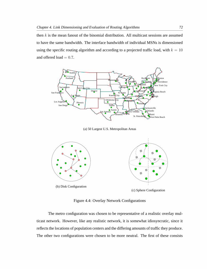
Chapter 4. Link Dimensioning and Evaluation of Routing Algorithms 72
then k is the mean fanout of the binomial distribution. All multicast sessions are assumed
to have the same bandwidth. The interface bandwidth of individual MSNs is dimensioned
using the specific routing algorithm and according to a projected traffic load, with k = 10
and offered load = 0.7.
San Francisco
Seattle
Portland
Los Angeles
San Diego
Chicago
Dallas
Houston
AtlantaPhoenix
DetroitCleveland
Minneapolis
Denver
St. Petersburg
CincinnatiSt. Louis
Kansas City
Sacramento
Virginia Beach
San Antonio OrlandoNew Orleans
Las Vegas
Salt Lake City
Boston
Charlotte
Buffalo
Austin
Memphis
Raleigh
Jacksonville
Oklahoma City
MiamiWest Palm Beach
New York City
Providence
Nashville
Rochester
(a) 50 Largest U.S. Metropolitan Areas
(b) Disk Configuration(c) Sphere Configuration
Figure 4.4: Overlay Network Configurations
The metro configuration was chosen to be representative of a realistic overlay mul-
ticast network. However, like any realistic network, it is somewhat idiosyncratic, since it
reflects the locations of population centers and the differing amounts of traffic they produce.
The other two configurations were chosen to be more neutral. The first of these consists

Chapter 4. Link Dimensioning and Evaluation of Routing Algorithms 73
of 100 randomly distributed nodes on a disk and the second consists of 100 randomly dis-
tributed nodes on the surface of a sphere. In both cases, all nodes are assumed to have
equal traffic densities. In the disk, as in the metro configuration, the MSN interface band-
widths must be dimensioned, but in this case it is just a node’s location that determines its
interface bandwidth. In the sphere configuration, all nodes are assigned the same interface
bandwidth, since there is no node that is more central than any other.
The three network configurations are illustrated in Figure 4.4. In all configurations,
the geographical distance between two nodes is taken as the cost of including an edge
between those nodes in the multicast session tree.
4.2.2 Comparison of Tree Building Techniques
In the previous chapter, we suggested three basic tree building techniques: selecting the
closest pair (CP), selecting the pair that minimizes the component diameter (CC), and se-
lecting the pair that minimizes the single tree diameter (CT). The iterative versions of these
algorithms, namely ICP, ICC and ICT, seek to satisfy the diameter bound by loosening
the degree assignment produced by BDA. In this section, we examine their performance
sensitivities to different diameter bounds and to the number of rounds allowed for degree
adjustment. The simulation uses the metro configuration as the network topology and a
session fanout of 10.
Figure 4.5 shows the session rejection rates versus the ratio of the diameter bound
to the maximum inter-city delay (5500 km). In this simulation, we allow each algorithm to
loosen the degree assignment as many rounds as possible, until it reaches the smaller of the
nodes’ degree bounds or k−1. The horizontal line labeled as BDA, shows the rejection rate
using the balanced degree assignment strategy, but ignoring the diameter of the resulting
tree.
As most of the large cities in this map are along the coastal areas, the majority of
the sessions will span across the continent. Therefore, it is difficult to find a multicast
tree for these sessions when the diameter bound is tight, resulting in very high rejection

Chapter 4. Link Dimensioning and Evaluation of Routing Algorithms 74
1 1.2 1.4 1.6 1.8 2Diameter Bound / Maximum Inter−city Distance
10−5
10−4
10−3
10−2
10−1
100
Rej
ectio
n R
ate
Offered Load = 0.75
ICPICCBCTICT
BDA
Figure 4.5: Sensitivity to DiameterBound
0 2 4 6 8 10Maximum Degree Adjustment Round
10−4
10−3
10−2
10−1
100
Rej
ectio
n R
ate
Offered Load = 0.75
ICPICCICT
Figure 4.6: Sensitivity to Degree Adjust-ment Round
rates for all algorithms. However, as the diameter bound is relaxed, the rejection rate
improves for all the algorithms, with the iterative algorithms all achieving essentially the
same performance for diameter bounds of more than 1.8 times the maximum inter-city
distance. At intermediate diameter bounds, the ICT and BCT algorithm performs better
than the ICC and ICP algorithms. This suggests that building from a single tree, as both
ICT and BCT do, is more effective in minimizing the tree diameter. The BCT algorithm
does not allocate its node degree before building the tree; rather, it seeks to maximize the
residual bandwidth as the algorithm progresses. For large diameter bounds, BCT is not
able to reduce its rejection rate as much as the algorithms using balanced degree allocation.
Figure 4.6 shows the rejection ratio versus the maximum number of degree adjust-
ment rounds allowed in ICP, ICC and ICT. The diameter bound is fixed at 8000 km for
this simulation. In each degree adjustment round, the number of vertices being adjusted
is 3. Generally, the ICP and ICC algorithms only benefit from the very first few rounds
of degree adjustment, which allows nearby nodes to be joined together to form collections
of small forests. The additional rounds of degree adjustment have no effect on them and
the rejection rates remain relatively high. Contrarily, the ICT algorithm benefits greatly
from the additional rounds of degree adjustment. It is able to utilize the increased degree
allocation at the centrally located nodes and form smaller diameter trees.

Chapter 4. Link Dimensioning and Evaluation of Routing Algorithms 75
We conclude in this subsection that the ICT algorithm, when combined with the
degree loosening procedure, is more effective at producing small diameter trees than ICP
and ICC when the diameter bounds are tight. In the rest of this paper, we will focus our
evaluation mainly on the ICT algorithm. However, ICT’s greater effectiveness comes with
a cost of added complexity, as it iterates through each possible starting vertex in order to
find the best tree. We will analyze the computational cost of the ICT algorithm later in the
section.
4.2.3 Performance Comparison on Session Rejection Rate
Figure 4.7 shows the session rejection rates versus offered load for a subset of the overlay
multicast routing algorithms presented earlier. The charts also include a lower bound on the
rejection fraction that was obtained by running a simulation in which a session is rejected
only if the sum of the degree bounds at all nodes in the network is less than 2(k − 1).
The lower bound curves are labeled LB. The results, labeled BDA, are obtained using the
balanced degree allocation strategy, and ignoring the diameter of the resulting tree. We
conjecture that this also represents a lower bound on the best possible rejection fraction
that can be obtained by any on-line routing algorithm. It is certainly a lower bound for
algorithms based on the balanced degree allocation strategy.
For these charts, the diameter bound for the metro configuration is 8000 km which
is approximately 1.5 times the maximum distance between nodes. For the disk and sphere
topology, the bound is two times the disk diameter and three times the sphere diameter;
each is about twice the maximum distance between any two nodes. The total interface
bandwidth for all MSNs is 10,000 times the bandwidth consumed by a single edge of a
multicast session tree. So, in the sphere, each MSN can support a total of 100 multicast
session edges and for the metro configuration, the average number is 200.
Overall, the results show that the algorithms that seek to balance the residual degree
usually perform much better than the CT algorithm, which merely seeks to minimize the
diameter subject to a constraint on the maximum degree bound of a node. The performance
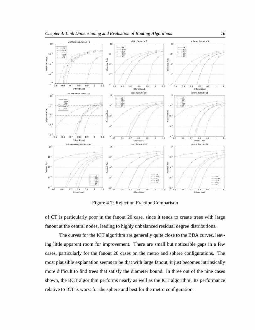
Chapter 4. Link Dimensioning and Evaluation of Routing Algorithms 76
0.5 0.6 0.7 0.8 0.9 1 1.1Offered Load
10−4
10−3
10−2
10−1
100
Rej
ectio
n R
ate
US Metro Map, fanout = 5
LBBDAICTBCTCT
0.5 0.6 0.7 0.8 0.9 1 1.1Offered Load
10−4
10−3
10−2
10−1
100
Rej
ectio
n R
ate
disk, fanout = 5
LBBDAICTBCTCT
0.5 0.6 0.7 0.8 0.9 1 1.1Offered Load
10−4
10−3
10−2
10−1
100
Rej
ectio
n R
ate
sphere, fanout = 5
LBBDAICTBCTCT
0.5 0.6 0.7 0.8 0.9 1 1.1Offered Load
10−4
10−3
10−2
10−1
100
Rej
ectio
n R
ate
US Metro Map, fanout = 10
LBBDAICTBCTCT
0.5 0.6 0.7 0.8 0.9 1 1.1Offered Load
10−4
10−3
10−2
10−1
100
Rej
ectio
n R
ate
disk, fanout = 10
LBBDAICTBCTCT
0.5 0.6 0.7 0.8 0.9 1 1.1Offered Load
10−4
10−3
10−2
10−1
100
Rej
ectio
n R
ate
sphere, fanout = 10
LBBDAICTBCTCT
0.5 0.6 0.7 0.8 0.9 1 1.1Offered Load
10−4
10−3
10−2
10−1
100
Rej
ectio
n R
ate
US Metro Map, fanout = 20
LBBDAICTBCTCT
0.5 0.6 0.7 0.8 0.9 1 1.1Offered Load
10−4
10−3
10−2
10−1
100
Rej
ectio
n R
ate
disk, fanout = 20
LBBDAICTBCTCT
0.5 0.6 0.7 0.8 0.9 1 1.1Offered Load
10−4
10−3
10−2
10−1
100
Rej
ectio
n R
ate
sphere, fanout = 20
LBBDAICTBCTCT
Figure 4.7: Rejection Fraction Comparison
of CT is particularly poor in the fanout 20 case, since it tends to create trees with large
fanout at the central nodes, leading to highly unbalanced residual degree distributions.
The curves for the ICT algorithm are generally quite close to the BDA curves, leav-
ing little apparent room for improvement. There are small but noticeable gaps in a few
cases, particularly for the fanout 20 cases on the metro and sphere configurations. The
most plausible explanation seems to be that with large fanout, it just becomes intrinsically
more difficult to find trees that satisfy the diameter bound. In three out of the nine cases
shown, the BCT algorithm performs nearly as well as the ICT algorithm. Its performance
relative to ICT is worst for the sphere and best for the metro configuration.

Chapter 4. Link Dimensioning and Evaluation of Routing Algorithms 77
Looking down each column, we see that the lower bound increases with the fanout.
This simply reflects the fact that each session consumes a larger fraction of the total in-
terface bandwidth. For the sphere, the rejection fraction also increases with fanout for the
BDA curve. This makes sense intuitively, since as the fanout grows, one expects it to be
more difficult to find balanced trees with small enough diameter. In the disk and metro con-
figurations, it is less clear why the BDA curve changes with fanout as it does. Part of the
explanation for the observed behavior is that the network dimensioning process is based on
an assumed traffic load, and in particular, an assumed multicast session fanout of 10. When
the simulated traffic has the same fanout distribution as the one used to dimension the net-
work, we get smaller rejection rates. However, there is a somewhat surprising deterioration
of the rejection rate for small fanout, particularly in the metro network case. The apparent
explanation for this is that with small fanout, we often get sessions involving MSNs near
the east and west coasts, but none in the center of the country. Such sessions are unable
to exploit the ample unused bandwidth designed into the more central MSNs, based on a
larger average fanout. A similar effect is observed with the disk, but it is more extreme in
the metro configuration because of the greater population densities on the coasts, and also
the smaller ratio of the diameter bound to the maximum inter-MSN distance (1.5 vs. 2).
0 5 10 15 20Routed Traffic Mean Fanout
10−4
10−3
10−2
10−1
100
Rej
ectio
n R
ate
20
3
5
10
15
Figure 4.8: Routing Performance over Differently Dimensioned Networks

Chapter 4. Link Dimensioning and Evaluation of Routing Algorithms 78
To further illustrate the effects of the traffic distribution used in network dimension-
ing on the routing performance, we ran a series of simulations on network configurations
that were dimensioned with different session fanout. In Figure 4.8, the x-axis shows the
mean fanout of the actual traffic and each curve is labeled by the mean session fanout used
during the dimensioning procedure. We used the BCT algorithms to route the sessions
here, but expect all algorithms to exhibit similar trends.
Figure 4.8 clearly shows that the best performance on each network configuration is
achieved when using the same fanout distribution for dimensioning and for routing, and that
the performance degrades when the session fanout deviates from the dimensioned fanout
in both directions. Since in reality, there may not be a single distribution that the session
fanout will follow, the best choice for dimensioning is to select the distribution that will
produce the widest range of small session rejection rate. Our choice of mean fanout of 10
is thus justified by coincidence.
4.2.4 Performance Comparison on Multicast Tree Diameter
Next, we investigate the performance of these algorithms in terms of the diameter of the
trees they created. Figure 4.9 shows the cumulative distribution of the tree diameter scaled
to the diameter bound used in the algorithms. The fanout used here is 10 per session. Also,
we show in a table the mean and variance of the tree diameter using unscaled values.
We observe that the diameter performance of the BCT algorithm is as good as that
of the CT algorithm; the difference is almost indiscernible. The ICT algorithm does, how-
ever, show a performance degradation on the tree diameter. Especially in the sphere, ICT
generates trees with diameters about 20% larger than those generated by the other two
algorithms. This is because traffic load tends to be more evenly distributed in the sphere
configuration and BDA is so effective at equalizing the available capacity at each MSN, that
it tends to produce degree allocations with large numbers of vertices of degree 2, resulting
in long paths.
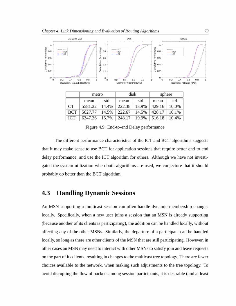
Chapter 4. Link Dimensioning and Evaluation of Routing Algorithms 79
0 0.2 0.4 0.6 0.8 1Diameter / Bound (8000km)
0
0.2
0.4
0.6
0.8
1C
umul
ativ
e P
erce
ntag
e
US Metro Map
ICTBCTCT
0 0.2 0.4 0.6 0.8 1Diameter / Bound (2*D)
0
0.2
0.4
0.6
0.8
1
Cum
ulat
ive
Per
cent
age
Disk
ICTBCTCT
0 0.2 0.4 0.6 0.8 1Diameter / Bound (3*D)
0
0.2
0.4
0.6
0.8
1
Cum
ulat
ive
Per
cent
age
Sphere
ICTBCTCT
metro disk sphere
mean std. mean std. mean std.CT 5581.22 14.4% 222.38 13.9% 429.16 10.0%BCT 5627.77 14.5% 222.67 14.5% 428.17 10.1%ICT 6347.36 15.7% 248.17 19.9% 516.18 10.4%
Figure 4.9: End-to-end Delay performance
The different performance characteristics of the ICT and BCT algorithms suggests
that it may make sense to use BCT for application sessions that require better end-to-end
delay performance, and use the ICT algorithm for others. Although we have not investi-
gated the system utilization when both algorithms are used, we conjecture that it should
probably do better than the BCT algorithm.
4.3 Handling Dynamic Sessions
An MSN supporting a multicast session can often handle dynamic membership changes
locally. Specifically, when a new user joins a session that an MSN is already supporting
(because another of its clients is participating), the addition can be handled locally, without
affecting any of the other MSNs. Similarly, the departure of a participant can be handled
locally, so long as there are other clients of the MSN that are still participating. However, in
other cases an MSN may need to interact with other MSNs to satisfy join and leave requests
on the part of its clients, resulting in changes to the multicast tree topology. There are fewer
choices available to the network, when making such adjustments to the tree topology. To
avoid disrupting the flow of packets among session participants, it is desirable (and at least

Chapter 4. Link Dimensioning and Evaluation of Routing Algorithms 80
for some applications necessary) to avoid large-scale changes to the tree topology. The
least disruptive approach is to add a new MSN, by just adding a connection between it
and another MSN that is already supporting the session. Similarly, a departing MSN is
removed from the tree when it no longer has any clients participating in the session, and it
is a leaf in the multicast tree. This approach ensures that packet flows are not disturbed by
membership changes. The requirement that an MSN with no clients, remain in a multicast
tree if it is not a leaf, is important for session continuity, but does have a negative impact on
overall network performance. This effect is quantified by the results presented below. We
also show that a significant improvement in performance can be obtained if an MSN with
no clients is permitted to drop out of a multicast tree if its degree in the tree drops to two.
For this case, we can make a simple adjustment to the tree topology that permits packet
flow continuity to be maintained, using special procedures for packet handling during the
transition.
When adding a new member to an existing multicast tree, we apply the same strategy
as the ICT algorithm. We first identify the set of nodes in the tree at which the addition of
an edge to the new MSN would not violate the diameter bound. We then add a connecting
edge at the node in this set with the largest residual degree. Ties are broken by selecting
the node that results in the smallest diameter tree.
We evaluate the performance of the ICT algorithm with dynamic sessions. The be-
havior of dynamic sessions depends largely on the applications. For example, a conferenc-
ing application may have a large number of members joining the session at the beginning
and staying throughout the session; while an on-line chat room may constantly have mem-
bers joining and leaving the session. Instead of conjecturing any specific models, we simply
start each session with a random initial session fanout selected from a binomial distribu-
tion and generate a number of join and leave requests uniformly distributed throughout the
session life time. In order to isolate the influence of session dynamics, we keep the average
session fanout constant at 10, which is the binomial mean that the network is dimensioned
with, by varying the mean of the initial session fanout distribution with linear projection of
the join and leave request rates. We use the tuple (initial fanout, number of join requests,

Chapter 4. Link Dimensioning and Evaluation of Routing Algorithms 81
0.5 0.6 0.7 0.8 0.9 1 1.1Offered Load
10−4
10−3
10−2
10−1
100
Ses
sion
Rej
ectio
n R
ate
US Metro Map
(10,0,0)(10,2,2)(10,4,4)(10,6,6)(10,8,8)(10,10,10)
0.4 0.6 0.8 1Offered Load
0
0.02
0.04
0.06
Fai
led
Join
Req
uest
s (10,2,2)(10,4,4)(10,6,6)(10,8,8)(10,10,10)
0.3
0.35
0.4
0.45
0.5
Def
erre
d Le
ave
Req
uest
s
Figure 4.10: Performance with Even Number of Join and Leave Requests
number of leave requests) to annotate each plot; the numbers for join and leave requests are
for each session.
Figure 4.10 shows the performance of the ICT algorithm with an equal number of
join and leave requests in each session. The plot shown in the left figure includes only the
fraction of sessions that are rejected at initialization; the fraction of rejected join requests is
shown separately in the right side bottom figure. As expected, the more dynamic addition
and deletion of tree branches there are, the worse the routing performance. The number
of failed join requests increases with the offered load, since at high load, join requests are
likely to arrive at nodes that are out of capacity. There are about 0.5% − 1% failed join
requests at the lightest traffic load for each session configuration. This is because a new
node, regardless of its location, always joins the tree as a leaf node. When a session is
initialized with nodes on both coasts only, a node in the more central location joining the
session tree is likely to add more distance to the tree diameter and to violate the diameter
bound (8000km). Regardless of the offered load, there are a small fraction of sessions that
have such configurations, resulting in the flat tails for all curves.
Overall, the fraction of failed join attempts remains small: with offered load equal
to 70%, there are no more than 1.5% failures. The top figure on the right side shows the
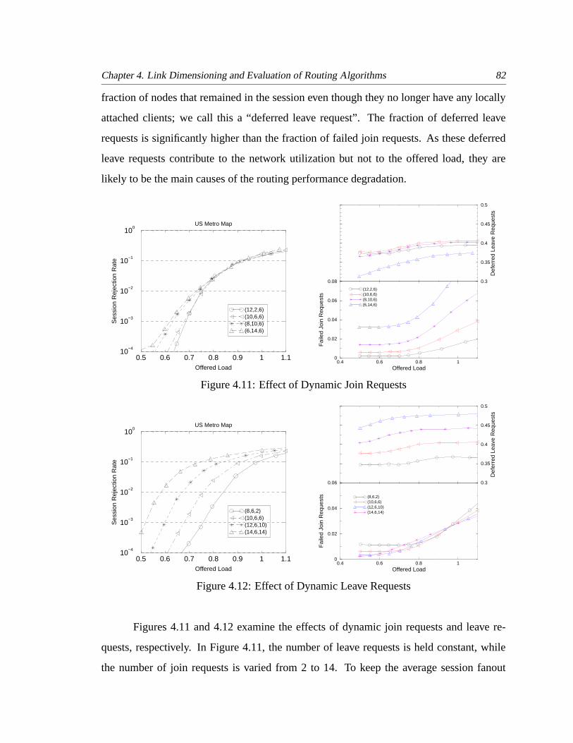
Chapter 4. Link Dimensioning and Evaluation of Routing Algorithms 82
fraction of nodes that remained in the session even though they no longer have any locally
attached clients; we call this a “deferred leave request”. The fraction of deferred leave
requests is significantly higher than the fraction of failed join requests. As these deferred
leave requests contribute to the network utilization but not to the offered load, they are
likely to be the main causes of the routing performance degradation.
0.5 0.6 0.7 0.8 0.9 1 1.1Offered Load
10−4
10−3
10−2
10−1
100
Ses
sion
Rej
ectio
n R
ate
US Metro Map
(12,2,6)(10,6,6)(8,10,6)(6,14,6)
0.4 0.6 0.8 1Offered Load
0
0.02
0.04
0.06
0.08
Fai
led
Join
Req
uest
s
(12,2,6)(10,6,6)(8,10,6)(6,14,6)
0.3
0.35
0.4
0.45
0.5
Def
erre
d Le
ave
Req
uest
s
Figure 4.11: Effect of Dynamic Join Requests
0.5 0.6 0.7 0.8 0.9 1 1.1Offered Load
10−4
10−3
10−2
10−1
100
Ses
sion
Rej
ectio
n R
ate
US Metro Map
(8,6,2)(10,6,6)(12,6,10)(14,6,14)
0.4 0.6 0.8 1Offered Load
0
0.02
0.04
0.06
Fai
led
Join
Req
uest
s (8,6,2)(10,6,6)(12,6,10)(14,6,14)
0.3
0.35
0.4
0.45
0.5
Def
erre
d Le
ave
Req
uest
s
Figure 4.12: Effect of Dynamic Leave Requests
Figures 4.11 and 4.12 examine the effects of dynamic join requests and leave re-
quests, respectively. In Figure 4.11, the number of leave requests is held constant, while
the number of join requests is varied from 2 to 14. To keep the average session fanout

Chapter 4. Link Dimensioning and Evaluation of Routing Algorithms 83
0.5 0.6 0.7 0.8 0.9 1 1.1Offered Load
10−4
10−3
10−2
10−1
100
Rej
ectio
n R
ate
US Metro Map (10,10,10)
with re−arrangementno re−arrangement
0.4 0.6 0.8 1Offered Load
0
0.02
0.04
0.06
Fai
led
Join
Req
uest
s with re−arrangementno re−arrangement
0.1
0.2
0.3
0.4
0.5
Def
erre
d Le
ave
Req
uest
s
Figure 4.13: Performance with Tree Re-arrangement
fixed, the initial fanout is varied. (Without this adjustment to the initial session fanout,
the average fanout would vary, clouding the meaning of the results, since the average ses-
sion fanout itself, has a significant effect on performance.) Similarly, in Figure 4.12, we
vary the number of leave requests from 2 to 14 while holding the number of join requests
fixed. Comparing Figure 4.11 and 4.12, we clearly observe that the performance degrada-
tion caused by the leave requests is much larger than that caused by the join requests. This
suggests two things. One is that the ICT algorithm can tolerate the less balanced bandwidth
usage caused by the incremental joins quite well. The other is that the restriction of only
allowing leaf nodes to drop out of a tree has a big effect on the overall performance. The
top curve in Figure 4.12 shows that nearly 50% of nodes remained in the session even when
they were no longer supporting any local clients. This suggests that it may be important to
allow some limited rearrangement following leaves.
Figure 4.13 shows how the performance changes when MSNs with no clients are
permitted to drop out of a multicast tree when their degree drops to two. The utilization at
which the session blocking probability is equal to 1% increases from about 65% to about
75%, suggesting that a network that allows limited rearrangement can carry about 15%
more traffic than a network that does not (assuming a target session rejection rate of no
more than 1%).

Chapter 4. Link Dimensioning and Evaluation of Routing Algorithms 84
4.4 A Hybrid Scheme To Reduce Complexity
Although the ICT algorithm gives superior performance on the overall system utilization
and can satisfy the diameter bound in most cases, it potentially has the disadvantage of
higher computational complexity. This is especially true with a more stringent diameter
bound, since in this case the algorithm continues to loosen the nodes’ degree allocation
over several rounds in order to find an appropriate tree.
0
0.1
0.2
0.3
Fra
ctio
n of
ses
sion
s fo
r re
laxa
tion
Computation Complexityfanout = 10, offered load = 0.75
1.5 1.6 1.7 1.8 1.9 2Diameter bound / Disk diameter
0
1
2
3
4
5
Ave
rage
rou
nd o
f rel
axat
ion
Figure 4.14: Computation Complexity of the ICT Algorithm
In Figure 4.14, we plot the computation requirement for the ICT algorithm on a disk
topology with session fanout equal to 10. The top half of the figure shows the percentage
of sessions that require degree adjustment; and the bottom half shows the average number
of rounds required for these sessions. We observe that the actual number of additional
rounds is reasonably low. For instance, if the diameter bound is 1.7 times the disk diameter,
10% of the sessions require an average of 2 rounds of degree adjustment. However, if the
diameter bound is too stringent, the extra rounds of degree adjustment do not help much in
reducing the session rejection rate (not shown). Therefore, it is important to pick a suitable
diameter bound for a topology so that the algorithm can operate more efficiently and more
effectively. From our experience, a bound of twice the maximum distance between all node
pairs is a good choice in all three network configurations.

Chapter 4. Link Dimensioning and Evaluation of Routing Algorithms 85
In order to reduce the computational complexity, we investigate a hybrid scheme
that combines the simplicity of CP and the ability of CT to find small diameter trees. The
hybrid scheme starts the same as CP, joining closest eligible pairs into components with
respect to the output of the BDA strategy. When there are g components left, the hybrid
scheme switch to the CT algorithm, joining the components by minimizing the multicast
tree diameter. The complexity of joining g components using the CT algorithm, is O(g2n2),
including the iteration of each component as the initial component. As before, the process
is repeated with rounds of degree loosening, until we find a multicast tree that satisfies the
diameter constraint.
0.5 0.6 0.7 0.8 0.9 1 1.1Offered Load
10−4
10−3
10−2
10−1
100
Rej
ectio
n R
ate
US Metro Map, fanout = 20
BDAICT hybrid, g = 4hybrid, g = 6hybrid, g = 10
0.5 0.6 0.7 0.8 0.9 1 1.1Offered Load
10−4
10−3
10−2
10−1
100
Rej
ectio
n R
ate
disk, fanout = 20
BDAICThybrid, g = 4hybrid, g = 6hybrid, g = 10
0.5 0.6 0.7 0.8 0.9 1 1.1Offered Load
10−4
10−3
10−2
10−1
100
Rej
ectio
n R
ate
sphere, fanout = 20
BDAICThybrid, g = 4hybrid, g = 6hybrid, g = 10
Figure 4.15: Performance of the hybrid CP and CT Algorithms
Figure 4.15 shows the performance of the hybrid scheme on three network topolo-
gies, with session size equal to 20. When g is small, the hybrid scheme inherits the same
problem as the ICP algorithm, and often fails to satisfy the diameter constraint. This is
especially true for the sphere configuration, where ICP tends to produce trees with many
nodes of degree 2, resulting in long paths in the tree. However, by increasing g, the hybrid
scheme gains quickly in its ability in finding a smaller diameter tree and brings down the
total rejection rate.
4.5 Implementation Cost
The computation of the ICT algorithm requires the global knowledge of the current residual
bandwidth of the participating MSNs. This information has to be updated periodically as

Chapter 4. Link Dimensioning and Evaluation of Routing Algorithms 86
each MSN participates in different sessions. In order to reduce the periodic broadcasting
of messages for state updates, we can use a larger update interval. However, this causes the
MSNs to route sessions based on imprecise information which consequently could cause
suboptimal routing and eventually reduce the total network utilization. Figure 4.16 shows
the trade-off between the routing update frequency and the network operational load for a
given rejection rate. The network configuration here is the metro topology and the session
fanout distribution has a mean of 10. The x-axis shows the ratio between the update fre-
quency versus the session arrival rate; the y-axis shows the maximum acceptable operating
load of the network for different target rejection rates. For instance, if the service provider
can tolerate a rejection rate of one every thousand sessions, we can operate at 75% of the
network capacity by sending updates at less than one tenth of the session arrival rate. As
expected, the operational load increases with the increase of the update frequency. Assum-
ing the overlay network accepts 100 sessions every minute, it will need to update routing
information every 6 seconds in order to operate at the 75% capacity. A state update mes-
sage contains the IP address of an MSN, its current residual bandwidth and a time stamp(or
sequence number) for a total of 12 bytes. The MSNs can have a separate multicast control
channel that includes all MSNs. Therefore, for 50 MSNs, the total message overhead is
12 ∗ 50 = 600 bytes for every 6 seconds.
0.01 0.1 1 = update frequency / arrival rate
0.2
0.4
0.6
0.8
1
Thr
esho
ld o
f Offe
red
Load 10
1010
−2
−3
−4
rejection rate
ε
no re−routingre−routing
target
Figure 4.16: Trade-off between NetworkOperating Load and Routing Update Fre-quency.
0.01 0.1 1 = update frequency / arrival rate
10
1
0.1
0.01
0.001
Re−
route
Sess
ions
(%)
10
10
10
−2
−3
−4
rejection rate
ε
Figure 4.17: Percentage of Re-routedSessions

Chapter 4. Link Dimensioning and Evaluation of Routing Algorithms 87
Imprecise routing information can cause routing sub-optimality as well as routing
failures. The host MSN can generate a multicast tree that exceeds another MSN’s residual
bandwidth, which results in session rejection. Straightforwardly, the MSNs can piggyback
their current residual bandwidth with their acknowledgment or rejection of a session, and
the host MSN can try to re-route the session based on this new information. The dashed line
curves in Figure 4.16 shows the network utilization with the re-routing attempt. For small
update frequencies, the re-routing helps to improve the operational load by as much 10%,
but is less successful for higher update frequencies. Figure 4.17 shows the corresponding
percentage of sessions that are routed the second time including both successful and failed
re-route attempts. There are at most one percent sessions that attempt to re-route, which
suggests that the majority of rejected sessions failed at the first routing attempt due to the
accumulated effects of routing based on imprecise information. As part of the future work,
we are looking into other update mechanisms to improve routing performance with smaller
update overhead.
4.6 Summary
In this chapter, we first introduced the dimensioning procedure which assigns bandwidth
capacity to individual MSNs according to their traffic load. The computation of the traffic
load requires three parameters: (1) a network topology; (2) a specific routing algorithm;
and (3) an assumed traffic distribution. By iteratively adjusting the bandwidth assignments,
the resulting configuration can achieve better routing performance. Based on this con-
figuration method, we evaluated the multicast routing algorithms over a variety of traffic
distributions and network topologies. We showed that ICT is the best algorithm for achiev-
ing the smallest session rejection rate and BCT is good at producing small diameter trees
and is the closest to ICT in achieving high overlay network utilization. Yet it can reject as
much as 20% more sessions than ICT in some network configurations. We also quantified
the ICT performance with dynamic session configurations and showed that in order to pre-
vent flow disruptions in dynamic sessions, the overlay utilization has to be sacrificed since

Chapter 4. Link Dimensioning and Evaluation of Routing Algorithms 88
some nodes that no longer have active local users, have to remain in the tree to support
the multicast session. Last, we investigated a hybrid scheme that can reduce computational
complexity for large sessions and achieves good overlay utilization.

89
Chapter 5
Placing Servers in Overlay Networks
In this chapter, we study another subproblem of the overlay network design problem: the
placement of the MSNs with constraints on the client to server paths, reflecting the quality
of service within the regional access networks. We envision that this imposition of service
quality constraints on server to client paths is essential for the newer network services to
achieve better service quality in order to attract and retain customers. While the server-
to-server paths can be explicitly provisioned in order to ensure available bandwidth and
routed to satisfy a delay constraint, this approach is generally not cost-effective on the
more numerous client access paths. Consequently, the quality of the service is determined
largely by network locations of the deployed servers. However, operating and maintaining
these distributed servers represents a major cost for service providers and limits the number
of servers that can be deployed.
To examine the trade-off between service quality and network cost, we ask the fol-
lowing question: Given multiple networks and their estimated service parameters, how
many servers are needed and where should an overlay service provider locate them to en-
sure a desired service quality to all its clients. The measure of quality of service can vary
from application to application: it can be delay for real-time applications, or bandwidth for
content distribution applications, or a combination of both. The connection from a client to
its designated MSN can stay within an ISP domain or may cross multiple domains. With the
emergence of co-location services in major metropolitan areas, we expect that fewer clients

Chapter 5. Placing Servers in Overlay Networks 90
would need to be routed through multiple ISPs to reach their designated MSNs. Within an
ISP network, the service provider can estimate these service quality parameters for a given
client to a potential server location based on the client’s network access technology and
the capacities of the internal routing paths. Across the ISP domains, such estimation is
also possible if the peering path between networks is explicitly indicated or if both net-
works guarantee a service level agreement from which we can infer the service parameters.
Therefore, we assume that we can decide in advance whether or not placing an MSN at a
specific location can provide a given client with the desired level of service quality. In the
rest of this chapter, we use regional routers from different ISP networks to represent the
aggregation of clients and use the network distance between a regional router and an MSN
as the service parameter, however, our methods can apply to any generic metrics.
To answer the above question, we transform the placement problem to the set cover
problem [14] and solve it using both linear programming (LP) relaxation and greedy heuris-
tics. An instance of the set cover problem is that given a base set of elements and a family of
sets that are subsets of this base set, find the minimum number of sets such that their union
includes all elements in the base set. The server placement maps to the set cover problem
as follows: an element corresponds to the network location of an edge router, which repre-
sents the aggregation of regional clients in an ISP network; The base element set contains
all the network locations of edge routers; A set represents a potential server placement at
one of the network locations; Each set includes all the network locations that are within the
service range from the server location represented by the same set. By solving the set cover
problem, we find the minimum number of servers and their locations, that will cover all
clients within the service range. We will only consider the uncapacitated version of the set
cover problem, where the servers do not have capacity limits and can serve as many clients
as possible. We think this uncapacitated version is adequate since it is typically cheaper to
buy more bandwidth at one location than to install a separate server. The set cover problem
is NP-Hard [42] and has approximation ratio of O(log n) [23,66]. We introduce a rounding
technique to solve the integer-programming formulation of the set cover problem based
on linear programming (LP) relaxation methods. The super-optimality of the LP problem

Chapter 5. Placing Servers in Overlay Networks 91
provides a lower bound to the IP formulation of the set cover problem. Using simulation,
we show that this rounding technique approaches the lower bound very closely; in fact, it
reaches the lower bound for a number of network configurations. Meanwhile, the greedy
heuristic also provides good performance in all instances with significantly less computa-
tion complexity.
One contribution of our approach is that we have investigated several variations of
the placement strategy and their associated costs. For example, what is the cost if each
client should be served by a backup MSN as well as a primary MSN? What is the cost if
backup MSNs are allowed to be placed at twice the range of the primary? What is the cost
saving if service range can be relaxed? Or if we can compromise the service quality of
some non-premier clients? Answers to these questions offers guidance to service providers
on the economy of their planned services. These different placement strategies can be
mapped to different node inclusion criteria when constructing a set, and we can then solve
the resulting set cover instances with the same algorithms.
Another important aspect of our study is the network modeling used in our simula-
tion. Existing network modeling tools, such as GT-ITM [89] and Tiers [20], can generate
hierarchical network graphs with probabilistic network interconnections, however, they do
not explicitly model the geographical locations of the network elements. In our model, we
consider the potential of co-located servers which can access multiple networks from the
same geographical location; this mirrors the behavior of co-location service providers in
the current Internet. Therefore, when two network nodes of different networks are within
a geographical vicinity, a server placed at this location can service clients who are within
the service range in both networks. We show that these co-locations can greatly reduce
the number of required servers, since they avoid long indirect paths through the network
peering points by providing shortcuts from one network to another.
The rest of the chapter is organized as follows: we introduce the formal problem
definitions and the algorithms in Section 5.1; we then describe the network models used
in our simulations in Section 5.2; Section 5.3 presents simulation results; Section 5.4 dis-
cusses some of the related work; and in Section 5.5, we summarize our results.

Chapter 5. Placing Servers in Overlay Networks 92
5.1 Formal definitions and the Algorithms
The transformation of the placement problem to the set cover problem assumes that we are
given a set of networks and their interconnections, as well as a specific routing policy that
allows us to compute an end-to-end path for every pair of nodes in the networks. Typically,
shortest path routing algorithm is used in intra-domain routing and for inter-domain traffic,
packet flows are routed towards the nearest peering point between two networks (also called
the “hot-potato” routing). With this routing policy, we can compute a routing table for each
node ni and the cost of each routing path c(ni, nj), which is the sum of the hop distances
along the path. For each node ni, we compute a set S which includes all the nodes reachable
from ni within the routing cost of C. This is to say that if a server is placed at the location
of node ni, then all the nodes within this set can be serviced by this server. If ni has
co-location nodes, then the set S also includes all nodes reachable from each of these co-
location nodes within the cost of C. By varying the criteria of including a node in a set, for
example varying the cost C changes the service range of a server, we can explore different
placement policies while using the same algorithms to find a solution for the set cover
problem.
Let S1, S2, . . . , Sm be all the sets computed. The LP formulation of the set cover
problem is:
Objective: minimizej=m∑
j=1
xj (5.1)
Subject to:j=m∑
j=1
aijxj ≥ 1 for i = 1 . . . n (5.2)
xj ∈ {0, 1}
where xj is the selection variable of Sj , aij is 1 if ni ∈ Sj and 0 otherwise.
A variation of the problem is to allow one primary and one backup server to cover
each node. A backup server can cover twice the distance of the primary server. Let

Chapter 5. Placing Servers in Overlay Networks 93
T1, T2, . . . , Tm be all the backup sets, and bij = 1 if ni ∈ Tj and 0 otherwise. The objective
here is still to minimize the number of selected sets but with the additional constraints of:
j=m∑
j=1
bijxj ≥ 2 for i = 1 . . . n (5.3)
Since all nodes in the primary set are also in the backup set centered at the same
server, bij = 1 if aij = 1; but we can not have a primary server also service the same node
as the backup server — the constraint in (5.3) ensures the selection of a different server as
the backup.
5.1.1 LP Relaxation-based Methods
The above formulation can be approximated by first solving the LP relaxation of the prob-
lem optimally and then rounding the fractional values to integers. The LP relaxation of the
problem is to allow the selection variables xj to take fractional values between [0, 1]. The
LP relaxation can be solved in polynomial time and the rounding can be done in O(n). Ref-
erence [33] introduced a rounding algorithm which is a p-approximation algorithm, where
p = maxi{∑
j aij} is the maximum number of sets covering an element. Although this
worst case result is not very promising, we are more interested in the average case perfor-
mance. We refer to the rounding algorithm in [33] as the fixed-rounding (FR) algorithm:
Step 0: Solve the LP relaxation of the problem
and let {x∗
j} be the optimal solution;
Step 1: Output sets = {j|x∗
j ≥1p}.
The intermediate solution for the LP relaxation naturally provides a lower bound
=∑
j x∗
j for the set cover problem, since the fractional solution is an optimal solution and
the LP relaxation is a super set of the set cover problem. We will use this lower bound to
evaluate the quality of the solutions produced by our algorithms.
We have also devised an incremental-rounding (IR) algorithm that imposes more
restricted rules while selecting sets based on the value of x∗
j . Whenever we select a set,
we remove all the elements that satisfy the covering constraint in (5.2) due to the newly

Chapter 5. Placing Servers in Overlay Networks 94
selected set. Let M denote the union of all elements covered after each step. For the
remaining uncovered elements in a set Sj , we compute pj = maxi{∑
j aij} for i ∈ Sj\M .
Among all the sets that have selection variables greater than the inverse of pj , we choose
the set that has the largest number of nodes that have not been covered.
Step 1: Solve the LP relaxation of the problem
and let {x∗
j} be the optimal solution;
Step 2: Select set Sj such that :
2(a) Sj has the largest number of uncovered element;
2(b) x∗
j ≥1pj
;
Step 3: Repeat step 2 until all elements are covered.
The correctness of the algorithm holds: for each uncovered node, at least one set
has x∗
j ≥ 1∑
jaij
and pj ≥∑
j aij . By selecting all sets whose values satisfy 2(b), we are
guaranteed to cover all the nodes. Further more, since pj is non-increasing in each repeti-
tion and pj ≤ p, the set selection criterion is more restrictive than that in the FR algorithm,
which in turn reduces the number of sets selected. Although the worst case bound is the
same for both algorithms, we observe from our simulations that the IR algorithm typically
performs much better than the FR algorithm.
An alternative to rule 2(a) is to select the set with the greatest x∗
j value, since the
larger the value of the selection variable, the more “essential” the set may be. For example,
if a node is covered by a single set, then the selection variable of this set must be 1 and
the set must be selected. However, most of our simulations show that rule 2(a) generally
performs better than this alternative rule. One plausible explanation is that rule 2(a) is
more objective in attempting to include as many uncovered nodes as possible, while the
alternative rule first selects those more “essential” sets, which may not contain many nodes.
It is easy to see that both of the algorithms can still have redundant sets in the final
solution. To prune these unnecessary extra sets, we use a simple pruning algorithm as the
final step to complete the set selection:

Chapter 5. Placing Servers in Overlay Networks 95
Step 1: Sort all selected sets in increasing order of set size;
Step 2: Starting from the smallest set, check if it can be removed
without leaving any of its nodes uncovered.
Step 3: Repeat Step 2 until all sets are checked.
5.1.2 Greedy Heuristics
A greedy algorithm is usually attractive due to its simplicity. In [41, 48], Johnson and
Lovasz introduced a greedy algorithm for the set cover problem with an O(log n) approxi-
mation ratio. The basic greedy attribute of the algorithm is to select a set at every step that
contains the maximum number of uncovered elements. For the backup problem variant,
we extend the algorithm by treating any node that has not satisfied the constraints of (5.2)
and (5.3) as equally uncovered. At each step, we select a set that has the largest number of
remaining uncovered nodes and repeat till there are no more uncovered nodes.
5.1.3 Comparison of the FR, IR and the Greedy Algorithms
We first compare our incremental rounding (IR) algorithm with the fixed rounding (FR)
algorithm proposed in [33] and with the greedy algorithm. The results are further compared
with the lower bound obtained as the optimal solution from the LP method. The LP solver
we used, is called PCx [18] which is an interior-point based linear programming package.
We use a simple setup to investigate the relative performance of these algorithms.
The underlying network graph is a single graph of randomly distributed nodes on a 100 by
100 unit length map. The service range of a server is 20 units. Ideally, if nodes are perfectly
positioned, this will give a solution of d 10040e × d100
40e = 9 selected servers regardless of the
node density. The lower bound we obtained is indeed not far from the ideal and stays
constant with increasing node density as shown in Figure 5.1.
We show the performance of the rounding algorithms with and without the prun-
ing routine in Figure 5.1. As expected, the FR algorithm performs badly with increasing
node density, since the largest number of sets covering a node p, also increases with node

Chapter 5. Placing Servers in Overlay Networks 96
0 200 400 600 800 1000Number of Nodes
0
20
40
60
80
Num
ber
of S
erve
rslower boundIRFRGreedy
(a) Performance without the pruning routine
0 200 400 600 800 1000Number of Nodes
0
5
10
15
20
Num
ber
of S
erve
rs
lower boundIRFRGreedy
(b) Performance with the pruning routine
Figure 5.1: Performance Comparison of the FR and IR Algorithms
density which makes the selection criterion less strict. On the other hand, the IR algo-
rithm is always the closest to the lower bound. The FR algorithm does benefit greatly from
the pruning routine, achieving performance closer to the lower bound, and is only slightly
worse than the IR algorithm, but better than the greedy algorithm. This relative perfor-
mance holds for other settings we have tried as well. In the rest of the Chapter, we will
mainly focus on the IR algorithm to evaluate the placement methods in more complicated
network configurations.
5.2 Network Models
We model the networks using two types of graphs: random graphs and geographic graphs.
The latter consists of network nodes within each of the 50 largest US metropolitan areas.
For inter-domain network connectivities, we specify a set of parameters to determine the
location and density of network peering points. For intra-domain network connectivities, as
ISPs are not willing to disclose fully their network topology, we assume that they are able
to engineer and operate their own networks with little or no congestion internally so that the
delays between the routers are dominated by the link propagation delay. Consequently, we

Chapter 5. Placing Servers in Overlay Networks 97
model the intra-domain network as a complete graph. We assume the “hot-potato” routing
policy at the inter-domain level, which minimizes the number of network domains crossed.
Hence, traffic destined to another domain is always sent to the nearest peering points from
the originator towards the destination domain. Although such policy does not result in
the best global routes, it is widely used by the current inter-domain routing protocol: the
Border Gateway Protocol (BGP) [67].
Our modeling choices do not correspond directly to the current Internet since the in-
formation needed to model geographically at the AS-level and the router-level networks is
not generally available. The Netgeo tool [81] from CAIDA is probably the best mechanism
available for capturing such data. It extracts information from the whois [30] database and
attempts to map Internet hosts according to their domain names. However, the accuracy
of this method is not at all clear since large IP address blocks can be assigned to a single
network entity, and there is the possibility of inconsistency among whois databases. Addi-
tionally, it is not possible to determine all the locations of network peering points as many
ISPs have private peering links in addition to their point of presence at the public peering
points such as the MAEs and NAPs. We detail our parameter choices for the two models
below and summarize the parameters in Table 5.1.
Table 5.1: Parameters for Generating Network GraphsParameters Meanings
n network size as # of nodesscale size of the network graphNp probability of a city in a networkTXp interconnection probability between two networksTXscope scope of a region possible for interconnectionTXds interconnection densityvicinity vicinity feasible for nodes co-location
Random Graph
In the random graph model, nodes are randomly distributed over a plane of size scale x
scale. The number of nodes in each network is uniformly drawn from the interval on [min,

Chapter 5. Placing Servers in Overlay Networks 98
max]. We divide the plane into fixed size regions according to the parameter TXscope. The
interconnection probability TXp decides if a pair of networks interconnect; we choose TXp
based on the size of the two networks:
TXp = αeβ√
n1n2
max
where n1 and n2 are the number of nodes in the two networks, α and β determine the scale
and shape parameters of the probability distribution, respectively. So, two large networks
are more likely to interconnect than two smaller networks.
If two networks interconnect, we randomly select a number of regions to intercon-
nect according to the interconnection density TXds. If there are multiple nodes from each
network in the same region, we select the closest pair of nodes; if a region is selected, but
one of the network does not have any node in that region, we choose another region until we
meet the peering density criterion, or we have considered all regions. We allow co-location
if nodes from different networks are within a geometric distance (the vicinity parameter)
of each other. A server placed at a co-location can send traffic to all these networks with
no additional cost.
Geographic Graph
In the geographic model, we use the 50 largest metropolitan areas as node locations. We
then divide the US continent into 5 regions, namely northeast, northcentral, southeast,
southcentral and west, and categorize nodes into regions with a certain amount of over-
lap. Unlike the random graph model where all networks share the same geometric space,
the geographic model consists of two types of networks: regional networks and national
networks. Each city joins the network with probability Np: the selection of nodes for a
regional network considers only nodes that belong to that region; while a national network
considers all 50 cities. As before, we interconnect two networks with probability TXp. The
values of TXp may be different depending on the types of the two networks. For example,
two national networks will have TXp = 1, since they are almost always interconnected;

Chapter 5. Placing Servers in Overlay Networks 99
while two regional networks are less likely to peer with each other directly but to transit
through a national network. We allow interconnections only if two network nodes are in
the same city and use TXds to decide the number of peering points of two networks.
Geographic Categorization of Metropolitan Areas
Region north central[17] = ”Chicago, IL”, ”Detroit, MI”, ”Cleveland, OH”,
”Minneapolis, MN”, ”St. Louis, MO”, ”Denver, CO”,
”Cincinnati, OH”, ”Kansas City, MO”, ”Milwaukee, WI”,
”Indianapolis, IN”, ”Columbus, OH”, ”Salt Lake City, UT”,
”Nashville, TN”, ”Memphis, TN”, ”Oklahoma City, OK”,
”Grand Rapids, MI”, ”Louisville, KY” ;
Region north east[21] = ”New York, NY”, ”Chicago, IL”, ”Washington, DC”,
”Philadelphia, PA”, ”Boston, MA”, ”Detroit, MI”,
”Cleveland, OH”, ”Pittsburgh, PA”, ”Cincinnati, OH”
”Milwaukee, WI”, ”Virginia Beach, VA” ”Indianapolis, IN”,
”Columbus, OH”, ”Charlotte, NC”, ”Greensboro, NC”,
”Buffalo, NY”, ”Hartford, CT”, ”Providence, RI”,
”Rochester, NY”, ”Raleigh, NC”, ”Richmond, VA” ;
Region west[10] = ”Los Angeles, CA”, ”San Francisco, CA”, ”Seattle, WA”,
”Phoenix, AZ”, ”San Diego, CA”, ”Denver, CO”,
”Portland, OR”, ”Sacramento, CA”, ”Las Vegas, NV”,
”Salt Lake City, UT”;
Region south central[12] = ”Dallas, TX”, ”Houston, TX”, ”Atlanta, GA”,
”Phoenix, AZ”, ”St. Louis, MO”, ”Kansas City, MO”,
”San Antonio, TX”, ”New Orleans, LA”, ”Nashville, TN”,
”Austin, TX”, ”Memphis, TN”, ”Oklahoma City, OK”;
Region south east[15] = ”Atlanta, GA”, ”Miami, FL”, ”St. Petersburg, FL”,
”Virginia Beach, VA”, ”Orlando, FL”, ”Charlotte, NC”,
”New Orleans, LA”, ”Greensboro, NC”, ”Nashville, TN”,
”Memphis, TN”, ”Raleigh, NC”, ”Jacksonville, FL”,
”West Palm Beach, FL”, ”Louisville, KY”, ”Richmond, VA”;

Chapter 5. Placing Servers in Overlay Networks 100
5.3 Simulation Results
It is challenging to select a representative set of simulations that demonstrate the relation-
ships between the methodologies, the configurations and the results, given the vast number
of parameters. In order to concentrate on a few aspects which we considered interesting,
we have mostly used small and uniform settings in the simulations presented in this sec-
tion. We do not claim our network models capture all the fundamental characteristics of
the Internet, but we believe that the combination of random networks and the geographic
networks provides a wide enough spectrum to give us some confidence in the general utility
of the methods. Throughout the section, readers are referred to Table 5.1 for the definitions
of the parameters. Unless otherwise mentioned, we use the following default parameter
values: the random graph scale is 100 by 100 units; the probability of network interconnec-
tion is 1.0 for both network configurations; the region size is 10 units and the co-location
vicinity is two units in the random graph; the probability of including cities in the regional
networks is 0.6 and 0.8 for national networks in the geographic networks.
5.3.1 Single Network
We first present results on a single network for both the random graph and the geographical
graph. Each result for the random graph is averaged over 10 runs, while the result for the
geographic graph is from a single run, since the node locations are all fixed.
Figure 5.2 shows the number of required servers when varying service range. In
general, both the IR and the greedy algorithm performs closely with the lower bound. With
increasing service range, the number of servers needed drops significantly. In most cases,
the IR algorithm outperforms the greedy algorithm.
Figure 5.3 shows the performance against the different service requirements. We
perform simulations on the following three scenarios: (a) k = 1, with only one primary
server required to cover each node; (b) k = 1 and requiring one backup server; (c) k = 1
with relaxation on the server to client distance. The last scenario allows a compromise on

Chapter 5. Placing Servers in Overlay Networks 101
0
10
20
30
40
10 20 50Service Range (unit)
Nu
mb
er o
f S
erve
rs
Lower Bound
LP (IR)
Greedy
(a) Single Random Network: n = 100, scale = 100, k = 1
0
4
8
12
16
20
400 800 1200
Service Range (km)
Nu
mb
er o
f S
erve
rs
Lower Bound LP (IR) Greedy
(b) Single Geographical Network: n = 50, k = 1
Figure 5.2: Variation on Server Service Range
the service standard for a limited number of clients. This allows service providers to be
more cost effective and not to install servers just for a few remotely located nodes. The
backup server range is twice that of the primary server for both networks. The relaxation
is done by including every node in at least l server sets, even if it is not within the range of
l servers. That is, if a node is in the range of l′ < l servers, we add it to the sets for the next
l − l′ servers that it is closest to.
Figure 5.3 shows that the addition of the backup servers only increases the number
of total servers slightly. The service range relaxation is also effective in reducing number
of servers to about 75% and 55% of the original number, with l = 3 and l = 5 respectively.
However, the relaxation is useful only when the service range is small. In Figure 5.3,

Chapter 5. Placing Servers in Overlay Networks 102
0
10
20
30
40
k = 1 k = 1, w/backup k = 1, l = 3 k = 1, l = 5
Nu
mb
er o
f S
erve
rs
Lower BoundLP (IR)Greedy
(a) Single Random Network: n = 100, scale = 100, range = 10
0
5
10
15
20
25
k = 1 k = 1, w/ backup k = 1, l = 3 k = 1, l = 5
Nu
mb
er o
f S
erve
rs
Lower Bound LP (IR) Greedy
(b) Single Geographical Network: n = 50, range = 400 km
Figure 5.3: Variation on Different Service Requirement
the service range is 10 units and 400 km in the two network configurations, which covers
about 7% and 8% of the maximum distance in their respective networks. If we double the
service range, we find that the relaxation becomes irrelevant since each node is likely to be
included in multiple sets already. Table 5.2 shows the average node to server distance with
and without the service range relaxation. Since there may be multiple servers covering a
node, we select the closest server when computing the distance. The result for the random
graph are the worst case among 10 runs. These results quantifies the compromises made to
service quality in order to reduce the server cost.

Chapter 5. Placing Servers in Overlay Networks 103
Table 5.2: Average Client to Server distanceRandom Graph (unit) Geographic Graph (km)
range = 10 range = 400 kmmean std. max mean std. max
l = 0 4.94 3.74 9.83 167.49 140.11 398.79l = 3 6.30 4.47 14.82 259.78 222.65 1013.42l = 5 8.45 5.56 25.36 304.69 238.59 1114.78
5.3.2 Multiple Networks
In this section, we study the relationships between server placement and the density of
network peering links. By “peering links”, we mean both the peering and transit relation-
ship between two ISPs. As these links aggregate and transport traffic from one domain
to another, their limited capacities contribute significantly to the user experienced network
congestion. Additionally, these network exchange points maybe located off the optimal
path, resulting in longer and more circuitous routes. One way to circumvent these conges-
tion points is to use co-location services, where servers can access multiple networks and
can route traffic directly to these networks without going through the exchange points. We
demonstrate the relative performance with and without server co-location in Figure 5.4.
Table 5.3: Number of Peering Links In UseRandom Network Geographic Network
Density 5 networkss, 100 nodes per network 5 regional, 1 national network, total 96 nodestotal links co-location no co-location total links co-location no co-location
0.2 83.05 22.16% 38.77% 11.6 17.24% 80.17%0.4 158.05 23.28% 37.52% 18.9 10.05% 82.54%0.6 238.60 21.42% 38.98% 27.4 6.20% 82.48%0.8 317.75 22.19% 35.22% 36.3 8.82% 90.36%1.0 410.1 21.24% 35.94% 45.2 7.30% 96.90%
For this simulation, we use two network configurations: one is constructed from 5
random graphs, the other is constructed from 5 regional networks and 1 national network in
the geographic model. Hereafter, we will use the term m-n to denote geographic networks
consisting of m regional networks and n national networks. We use TXp = 1, so every
pair of networks is always interconnected, unless they do not have any common presences

Chapter 5. Placing Servers in Overlay Networks 104
0
10
20
30
40
50
60
0.2 0.4 0.6 0.8 1Peering Density
Nu
mb
er o
f S
erve
rs
LB with co-location IR with co-location IR no col-location
(a) Random Network: 5 networks, 100 nodes per network, range = 20,TXscope = 10, vicinity = 2
0
5
10
15
20
0.2 0.4 0.6 0.8 1
Peering Density
Nu
mb
er o
f S
erve
rs
LB with co-location IR with co-loation IR no co-location
(b) Geographic Networks: 5 regional networks, 1 national networks, totalnodes = 96, range = 800 km
Figure 5.4: Variation on Network Peering Density
in any of the peering regions. The peering density in Figure 5.4 determines the number of
peering points of two networks.
Figure 5.4 shows the number of required servers for the lower bound with co-
location and the IR algorithm with and without co-location. The co-location service re-
duces the number of required servers by as much as 50% when peering is sparse. The
geographic graph appears to be more sensitive to the peering density, as the performance of
IR with no collocation approaches the lower bound when the peering density approaches 1.

Chapter 5. Placing Servers in Overlay Networks 105
This is because the peering link is “cheaper” in a geographic network than in a random net-
work. In the geographic network, two networks peer only if they both have presences in the
same metropolitan area, which results in the delay on the peering link being zero. Contrar-
ily, the peering link has a positive delay in the random graphs which adds to the server to
client delay. Additionally, the “hot-potato” routing policy always selects the closest peering
link rather than the one with the lowest delay. These combined effect determines that the
increased peering density in random networks does not help much in reducing the server
cost. Table 5.3 summarizes the number of links used in the two scenarios. In the random
graph, the percentage of peering links in use stays almost constant; even more of them are
available with increasing peering density. On the other hand, large percentages of peering
links are in use in the geographic network when no co-location is allowed. The results for
the case of co-location show that only a very small number of peering links are needed if
servers are able to access multiple metropolitan area networks.
0.2 0.4 0.6 0.8 1Peering Density
1
1.5
2
2.5
Per
form
ance
Rat
io
net 2net 5net 10
no colocation
colocation
(a) Random Network: range = 20, vicinity =2, 100 nodes per network.
0.2 0.4 0.6 0.8 1Peering Density
0.5
1
1.5
2
2.5
Per
form
ance
Rat
io
net 5−1, colocnet 5−1, no colocnet 0−2, colocnet 0−2, no coloc
(b) Geographic Networks: range = 800 km.
Figure 5.5: Relative Performance Ratio Against Lower Bound
Figure 5.5 shows the relative performance ratio of the IR algorithm, with and with-
out co-location, against the lower bound. This is the same measure as those in Figure 5.4
but with more varieties on the network configuratons. We varied the number of random
networks as 2, 5 and 10 and used two configurations for the geographic networks: 5-1 and

Chapter 5. Placing Servers in Overlay Networks 106
0-2. The results are mostly consistent with that in Figure 5.4. Additionally, it suggests that
the performance of non co-located servers can degrade greatly with the larger number of
networks.
5.3.3 Server Load
Throughout this chapter, we assumed that the cost of installing and operating a separate
server far out weights the cost of buying more bandwidth at a location. We are also in-
terested in the distribution of load among the servers, particularly the minimum load on a
server, since it is not very cost-effective to install a server only to operate under very small
load.
Figure 5.6 shows the average and minimum server load distribution under the IR
algorithm with co-location. As expected, the average server load increases with the increase
of service range. The load distribution is more even on the random networks than on the
geographic networks due to the different node distribution: the geographic networks have
significantly higher population density on both coastal areas which creates higher load for
servers.
10 15 20 25 30Service Range (unit)
0
0.02
0.04
0.06
Fra
ctio
n of
Clie
nts
l = 0, average loadl = 0, minimal loadl = 5, average loadl = 5, minimal load
(a) Random Network, 5 nets, 100 nodes pernetwork, peering density = 0.4.
400 600 800 1000 1200Service Range (km)
0
0.1
0.2
0.3
0.4
Fra
ctio
n of
Clie
nts
l = 0, average loadl = 0, minimal loadl = 5, average loadl = 5, minimal load
(b) Geographic Networks, 5-1 nets, total 96nodes, peering density = 0.4.
Figure 5.6: Characteristics of Server Load

Chapter 5. Placing Servers in Overlay Networks 107
However, the minimal load does not lift as much for both networks. It is easier to
understand this effect in the geographic networks, since a few metropolitan areas, such as
Seattle and Portland, are more segregated from the rest of the areas. Consequently, it takes
at least one server to cover and only cover these two areas. Although it is less obvious
in the random networks, it seems that there are always a small number of nodes that are
particularly far away from the rest of the group. The curves labeled l = 5 indicate the
average and minimal fraction of clients served by a single server when we enforce each
node to be included in at least 5 server sets. The increase of the minimal server load from
the relaxation is more visible in the geographic networks than in the random networks.
5.4 Related Work
The application of the set cover problem in network design has two variants: the facility
location problem and the k-median problem. The facility location problem minimizes the
joint cost of server installation and the cost of connecting each client to its designated
server. This problem has been applied to designing and placing network concentrators. The
k-median problem minimizes the cost of connections between clients and servers under the
constraint that no more than k servers can be used. Both problems are NP-Hard. The best
known approximation algorithms can achieve constant ratio [28, 38, 78], if the connection
cost is symmetric and satisfies the triangle inequality. For arbitrary cost, the worst case
bound is O(log n). However, neither of the problems can be applied directly to the design of
overlay networks, since in the overlay model the communication channels between clients
and servers are over the commodity Internet and do not incur any cost to service providers.
Rather, the major cost is the number of servers needed to service all clients and the access
bandwidth required at each server’s network interface.
Our model of server placement more closely resembles the set cover problem. The
classic greedy algorithm for solving the set cover problem [41, 48] achieves an O(log n)
performance ratio. In geometric spaces, the problem is easier. In [35], Hochbaum proposed

Chapter 5. Placing Servers in Overlay Networks 108
a shifting strategy that gives an O(1 + ε) performance ratio. Unfortunately, the intercon-
nections between networks dictate that the network propagation delay no longer exhibits
the geometric properties of distance.
References [60,61] studied the problem of placing cache replicas in the network and
formulated it as the k-median problem: given a specific number of servers, what is the best
placement that achieves the highest average service level to clients, where service level is
indicated by access delay from a client to its nearest replica. In [60], Qiu et al. proposed
several placement strategies including: a greedy strategy that incrementally places replicas
to achieve highest service quality; a hot-spot strategy that places replicas near the clients
that generate the greatest load. In [61], the authors also proposed a max degree strategy by
placing replicas in decreasing order of nodes’ degrees. By simulating over several synthetic
and real network graphs, they concluded that the greedy strategy performs remarkably well,
achieving within 1.1 to 1.5 of the lower bound.
Our approach to network design is from a different angle. we are more interested
in examining the necessary cost, in this case the number of servers, if we want to provide
all clients the guaranteed service. This gives service providers insight into the relation of
network cost and the achievable service quality. Then, they can make adjustments to reflect
their revenue stream, such as eliminating servers that are only serving small numbers of
clients. Contrarily, the work in [60, 61] measures the average service quality which masks
the number of unhappy customers. Additionally, the performance of our approach, which is
the number of required servers, is not susceptible to the cost metric of connections, since we
only use it to categorize clients as serviceable or not by a server; while theirs is achieved for
a specific cost metric, namely the access delay. Since the connection cost metric depends
heavily on the application, it is not known if the same ratio could be achieved.
Another difference is that we model the network geographically and consider server
co-locations. As networks overlap geographically, the number of potential server locations
is much fewer in number than the number of network nodes that need to be considered.
In [60,61], they used network graphs consisting of tens of thousands nodes for router-level
graphs and thousands of nodes for AS-level graphs. Consequently, the optimal algorithm

Chapter 5. Placing Servers in Overlay Networks 109
based on LP relaxation is too expensive for their models. We think considering the ge-
ographical locations of servers is important and corresponds to the current trend in the
Internet, where servers are typically located in data centers in different geographic areas.
This reduces the problem size and enables us to solve it more optimally. In Section 5.3, we
compare the performance of our algorithm both with co-location and without, and show
that with co-location we can reduce the number of required servers to approximately half
of that with no network co-locations.
5.5 Summary
We have presented a server placement method in overlay networks as an application of the
set cover problem. The placement satisfies constraints on the server to client paths, which
indicate the achievable service quality along the path. We expect that network provisioning
for quality of service will become more common as the Internet continues to grow; and
such an automated methodology is useful for service providers to analyze the potential cost
of network provisioning.
We solved the set cover problem using methods based on linear programming re-
laxation as well as greedy heuristics. We also presented an incremental integer rounding
algorithm for the LP-relaxation based method. Our network settings model explicitly the
presence of co-location services, which have become increasingly popular for business cor-
porations to out source their data servers. Our results indicate co-location can save up to
50% of the server installation cost. We also presented variants of the simple set cover
problem to allow backup servers and to allow distance relaxation. These variances brings
opportunities to provide more cost effective services. Through simulation, we studied the
behavior of the algorithms under various network settings and observed the implication of
network peering density and the characteristics of server load distributions. Although, LP-
relaxation based methods are traditionally considered as too expensive and complex to use
in more time-critical contexts, we found that it is suitable and effective for overlay network
design where the solution quality is more important than the running time.

110
Chapter 6
Multicast Service in End-systems
The AMcast concept seeks to provide a global service network that can provide perfor-
mance improvements to group communication applications. These benefits are most sig-
nificant for applications that transmit at high data rates or have a large number of partic-
ipants. Consequently, it can be worthwhile for customers to pay their service providers
for obtaining these multicast services. There are, however, some circumstances where the
benefit of an AMcast service may not justify its cost to the users. These occasions occur
when an application only involves a small number of group members or operates within
a high bandwidth subnet, such as a campus network or corporate network. For example,
if a multi-player game session within a campus network were to use AMcast, each packet
would have to traverse back and forth on the link between the campus network to the ISP
network where the closest MSN is located. This creates additional bandwidth usage on the
access links where resource availability is often most limited. Another example is a set of
distributed cache servers that periodically require cache synchronization and update. As
these caches are likely to be geographically dispersed and have high speed network access
just as the MSNs do, the potential benefits of having the MSNs to tunnel traffic among
them in a timely manner diminishes in these respects. On the other hand, these applica-
tions can still benefit greatly from having multicast capabilities although the gains may not
be so much in reducing the network overhead from the unicast mechanisms, but in that

Chapter 6. Multicast Service in End-systems 111
the multicast mechanism can help the data sources to reduce the transmission load on their
CPUs and on their interfaces.
The potential of having thousands of such small group multicast applications exist-
ing simultaneously is not well-suited for the IP multicast model. The need for global IP
multicast addresses and the lack of a scalable address allocation scheme makes it unlikely
that IP multicast will be adopted by these applications. Therefore, we need a solution for
multi-sender multicast communication which scales for a large number of communication
groups with small numbers of members, and does not depend on multicast support in the
routers. In this chapter, we introduce an application level multicast infrastructure (ALMI)
that addresses these concerns. This solution provides a multicast middleware which is
implemented within the end systems and is capable of organizing the participants of a mul-
ticast session into a virtual multicast tree, i.e. a tree that consists of unicast connections
between end hosts. The tree is formed as a Minimum Spanning Tree (MST), where the cost
of each link is an application specific metric. Application level multicast offers acceler-
ated deployment, simplified configuration and better access control at the cost of slightly
higher traffic load in the network than native multicast. Since application level multicast is
implemented in user space, it allows more flexibility for customizing certain aspects, e.g.
data transcoding, error recovery, flow control, scheduling, differentiated message handling
or security, on an application-specific basis.
The rest of the chapter is organized as follows: section 6.1 presents the architecture
of the multicast middleware; section 6.2 presents operations that manages session member-
ship and the multicast tree; in section 6.3, we discuss several application-specific compo-
nents in ALMI; in section 6.4, we present the implementation of a Java based middleware
package and the results of some performance experiments conducted over a local area net-
work as well as over the Internet.

Chapter 6. Multicast Service in End-systems 112
6.1 Architecture Overview
An ALMI session consists of a session controller and multiple session members, shown in
Figure 6.1. The session controller is a program instance, located at a place that is easily
accessible by all members. It may be co-located with one of the session members, typ-
ically the session initializer, or it could reside on a special purpose server or a multicast
proxy installed within a corporate or an ISP network. Session members are organized into
a multicast tree. A link in the multicast tree (solid line) represents a unicast connection
between two members. Session data is disseminated along this multicast tree, while con-
trol messages are unicast between each member and the controller. The multicast tree is a
shared-tree amongst members with bi-directional links. In order to avoid loops, two mem-
bers incident on a link receive a designation of parent and child. This parent-child relation
distinguishes the two member for control purposed, as we will explain later in the section;
it does not indicate the direction of a data flow.
Member
Virtual
Multicast
Tree
ControllerSession
Figure 6.1: ALMI Architecture Overview
The session controller handles member registration and maintains the multicast tree.
In order to achieve the latter, the controller performs two important functions:
• It ensures connectivity of the multicast tree when members join and/or leave the
session and when network or host failures occur.

Chapter 6. Multicast Service in End-systems 113
• It ensures the efficiency of the multicast tree by periodically calculating a minimum
spanning tree based on the measurement updates received from all members. To
collect measurements the controller essentially instructs each member to monitor a
set of other members.
A session member receives and sends data as it would in an IP multicast session; in
addition, it also forwards data to designated adjacent neighbors. Data eventually reaches
all session members through this relaying process in a cooperative fashion. Besides for-
warding data on the data plane, a session member also monitors the performance of unicast
paths to and from a subset of other session members. This is achieved by periodically
sending probes to these members and measuring an application level performance metric;
in the current implementation the roundtrip response delay. Delay measurements are then
reported to the controller and serve as the costs used to calculate a Minimum Spanning
Tree.
Depending on the application, data transfer between two adjacent members can be
reliable or unreliable by deploying TCP (e.g. data replication services) or UDP (e.g. stream-
based applications), respectively. There are clear advantages in being able to use existing,
widely deployed protocols: first, it reduces system administration and configuration cost;
and second, use of TCP and its associated congestion mechanism offers hop-by-hop reli-
ability and provides compatibility in bandwidth sharing with regular flows. We stress that
the last property is rather convenient since multicast congestion control is an extremely hard
problem especially with respect to deployment viability. Additionally, applying TCP on a
hop-by-hop basis implicitly creates back pressure for the source to slow down, resulting in
end-to-end, albeit simplistic, congestion management.
ALMI takes the centralized control approach to maintaining tree consistency and
efficiency. This design choice was made for better reliability and reduced overhead during
a change of membership or a recovery from node (i.e. end system) failure. On the other
hand, the session controller operates only in the control path, and does not obstruct high
data rate transmissions among session members. We believe this centralized approach is
adequate and efficient for a large range of multicast applications. However, a centralized

Chapter 6. Multicast Service in End-systems 114
controller architecture has obvious implications in control plane reliability and fault toler-
ance. Clearly, a single controller would constitute a single point of failure for all control
operations related to the group. Two points should be made in this respect. First, the
centralized session controller could be augmented with multiple back-up controllers, op-
erating in “stand-by” mode, with addresses that are well known to all session members.
In this case, the “stand-by” controllers periodically receive state from the primary con-
troller, which would include recent measurements, tree topology and current membership
information. Second, even in the event that no control operation is possible, the existing
ALMI tree, and hence data path, will remain unaffected and will continue operation until a
membership change or a critical failure occurs. Therefore a transient controller (or its net-
work) failure can be tolerated. In summary, we believe the benefit of simplicity offered by
the centralized controller approach far outweigh any negative implications from the fault
tolerance perspective.
6.2 Protocols and Operations
An ALMI controller is identified by its IP address and a port number known to the ses-
sion members. For each new session, a controller randomly selects a session ID that is
locally unique. This session ID is used to demultiplex control flows received from different
sessions.
A session member is identified by its network address and the port number which
it uses to send control messages. The data path and control path at a session member is
separated by using different port numbers. Different session instances on an end system
use different port numbers for their session traffic. No further demultiplexing is necessary
once the ports are bound to the sessions.
A common packet format used to carry both data and control packets is shown in
Figure 6.2.

Chapter 6. Multicast Service in End-systems 115
Protocol Version FlagsTree Incarnation
Source ID
ALMI Session ID
Sequence Number
0 7 15 31
20 bytes
Payload Data Length
Figure 6.2: ALMI Packet Header Format
The content of this packet header is rather straight forward. The Session ID and
Source ID are generated by the controller and are guaranteed to be locally unique. The flag
field in the header defines various types of operational messages, including:
• Registration messages addressed from members to the controller. These messages
allow members to join, leave and re-join a session.
• Connection request and acknowledgment between parent and child. This message
exchanges parent and child data port information for establishing data connections.
• Performance monitoring messages reported from members to the session controller,
such as pairwise delay measurements between group members. These messages are
used by the controller to compute the session multicast tree.
• Distribution tree messages, generated by the controller, are used to inform members
of their peering points in the data distribution tree. This message informs members
of the IDs of their new parent and children. It typically occurs after detection of
network or system errors, or after a tree transition.
• Neighbor monitoring update messages, which are sent by the controller to members
to inform them of a new list of neighbors they need to monitor. This message is
triggered if the controller detects that the number of current monitoring pairs has
dropped below a threshold due to accumulated network errors.

Chapter 6. Multicast Service in End-systems 116
• Departure messages, are sent from group members to the controller and their current
parent and children. If a child member receives such a message from its parent, it
needs to contact the controller again to rejoin the group.
The Tree Incarnation field is to prevent loops and partitions in the multicast tree.
Since a session multicast tree is calculated centrally by the controller, assuming correct
controller operation, a loop free topology will always be generated. However, since tree
update messages are independently disseminated to all members, there is always a possibil-
ity that some messages might be lost or received out-of-order by different groups members.
In addition members might act on update messages with varying delay. All of these events
could result in loops and/or tree partition. In order to avoid these transient phenomena,
the controller assigns a monotonically increasing version number to each newly generated
multicast tree. To avoid loops, a source generating packets includes its latest tree incarna-
tion in the packet header. In order to guarantee tree consistency and ensure the delivery
of most packets while the tree is being reconfigured, each ALMI node maintains a small
cache of recent multicast tree incarnations. Thus, an ALMI node simultaneously keeps
state about multiple trees, each with the corresponding list of adjacent nodes. The number
of cache entries is configurable. When receiving a packet with a tree version contained in
the cache, the receiving node forwards it across the interfaces corresponding to this tree
version. Packets with old tree versions not contained in the cache are discarded. On the
other hand, if a member receives a data packet with a newer tree version, it detects that its
information is not up to date and therefore re-registers itself with the controller to receive
the new tree information.
Components Software Architecture
Figure 6.3 illustrates the system architecture for an ALMI controller and an ALMI member.
A controller receives control messages from session members through its well-known UDP
port. It maintains a hash table for quick lookups of session IDs and demultiplexes packets to
the session object for tasks like adding and deleting a member, or updating the connection

Chapter 6. Multicast Service in End-systems 117
Session 1 Session 2 Session n
Session
Timer
TableHas
htab
leS
essi
on ID ALMI
Controller
lookup() expire()
......
UDP Port
recv() send()
Datagram Socket
(a) Controller Architecture
receive()
setReliable()
send()ALMI Member API
Buffer
ForwardList
Data
Monitor ListNeighbor
Datagram Socket
TableEvent
ALMI Member
Receiver Thread
UDP Control TCP Listener
Receiver Thread Group
UDP Data
Receiver ThreadThreadTCP Data
CO
NT
RO
L
DA
TA
init()join()
leave()
Datagram socket Sever Socket Sockets
(b) Member Architecture
Figure 6.3: ALMI Components Architecture
monitoring statistics. Each session is associated with a timer which expires upon events
such as the periodic computation of the multicast tree and the detection of member failures.
An ALMI member has separate paths for data and control messages, and each path
binds with a separate port. A member maintains two lists: the neighbor monitoring list and
the packet forwarding list. The neighbor monitoring list consists of all other members that
are actively monitored by this node, which contains all or a subset of all session members.
The forwarding list consists of the adjacent members in the multicast tree where the packets
are to be forwarded. The event table triggers events such as sending out ping messages to
monitor connection performance, and other error recovery events which we will describe
later. An ALMI node maintains a data buffer that allows asynchronous data reception at the
application layer. When a node receives a data packet, it appends the packet in the buffer
and notifies the application. The buffer is cleared when a recv() call is initiated by the
application. If the buffer is full, the receiving thread will block and wait for the application
to clear the buffer.
There is an issue as to whether blocking at one application node should affect the
forwarding of data downstream from this node; in other words, whether the node should
stop forwarding or continue forwarding data when the application fails to clear the buffer
at its current pace. For adaptive applications, where the data source adapts its data rate

Chapter 6. Multicast Service in End-systems 118
to the slowest receiver rate, suspension of data forwarding could create “back pressure”
towards the source and allows the source to detect the congestion faster. On the other hand,
streaming applications may find it unacceptable to block due to a single slow node. The
problem of how to coordinate the data rate in a multicast session remains an open issue at
this point.
Next, we describe the main operations in an ALMI session. These operations han-
dle tasks related to membership management, performance monitoring and multicast tree
construction and update. ALMI uses UDP for messages exchanges on the control paths.
Since UDP does not guarantee to deliver the packets reliably, higher level mechanisms are
used to detect packet losses typically by the use of timers.
6.2.1 Session Membership Operations
Joining a session
A session member locates the session controller and obtains session information including
the session ID, the controller’s address and port number through offline channels such as a
URL, a directory service or an email message. It then opens a local UDP port for sending
session control messages. The first message it sends out, is a JOIN message to the controller
which indicates the session it wishes to join and includes its IP address and the control port
number. The controller finds the session information from its session table and creates a
new entry for the member. It then selects an existing member as the parent of the newly
joined member and returns a JOIN ACK to the member including the identification of the
parent member.
Establishing data connections
Next, the session member attempts to establish the data connection with its parent. To do
this, it sends a GRAFT message to the parent, which includes its own identification (IP
address and control port number) as well as the data port number. Depending on which
transport protocol is used in the session, the data port could be a UDP port (if UDP is

Chapter 6. Multicast Service in End-systems 119
in use) or a TCP listen port (the port that TCP uses to accept connections). The parent
member receives the message and creates a new entry in its neighboring list for monitoring
the connection performance and in its routing table for forwarding future data packets. It
then returns a GRAFT ACK containing its own information and the child creates similar
entries in its local tables.
When TCP is used, a connection has to be established between two adjacent nodes
with one end initiating and the other end accepting the connection. Therefore, the ALMI
controller assigns parent and child labels to two adjacent nodes: a TCP connection is always
initialized in the direction from a child to the parent. An additional step is then taken by the
child member to send a TCP SYN packet to the parent. Once the connection is established,
each member forwards data to all adjacent members, including all children and the parent,
except the one from which data is received.
Leaving a session
A member may leave any time during a session, voluntarily or involuntarily. When the
application decides to leave the session, a LEAVE message is sent to the controller, and to
its parent and all children nodes. The controller then switches the children nodes, if any, to
be the children of the parent of the leaving node. Or if the leaving node is the root of the
tree, one of the children nodes is selected as the new root and the rest, its new children. If
a member is involuntarily leaving the session, i.e. under the condition of a network failure,
the controller and its adjacent nodes detect the failure through timeouts and reconstruct
the tree with the same rules as if the member had left the session voluntarily. The re-
establishment of data connections between the new parent and child is the same as that in
the join procedure.
Since ALMI uses centralized control to construct the multicast tree, access control
modules can be easily integrated into the current software structure. The controller will
hold the ultimate authority as whether a node is allowed in the session or not by including
or excluding the node during the tree computation.

Chapter 6. Multicast Service in End-systems 120
6.2.2 Multicast Tree Management
We now turn to the computation of the ALMI distribution tree. A session multicast tree
is formed as a virtual Minimum Spanning Tree that connects all members. The minimum
spanning tree calculation is performed at the session controller and results are communi-
cated to all members in the form of a (parent, children) list. Link costs are representative of
an application specific performance metric which is computed by members in a distributed
fashion and reported to the controller periodically. In our current implementation, we use
roundtrip delay, measured at the ALMI layer, as the metric because latency is important
to most applications and is also relatively easy to monitor. However, some applications
may find other metrics, such as available link bandwidth, more appropriate. For example,
a bandwidth intensive application may prefer a high bandwidth, high delay link to a low
delay, low bandwidth link to carry its traffic. While the current version of ALMI does not
include the more sophisticated tools needed to measure available bandwidth, it is structured
to allow such tools to be easily inserted, so that alternative metrics can be used. In the rest
of this section, we will simply use delay as the default performance metric.
End-system Monitoring
In order to obtain monitoring results, ALMI connects all group members into a monitoring
graph. Members send ping messages to measure round trip delay to their neighbors in the
graph. For small groups, it is possible to create a mesh and have O(n2) message exchanges
to compute the best multicast tree. However, as group size grows, it becomes unscalable
to have a large number of message exchanges since the monitoring process is periodic and
continuous through the whole multicast session. To reduce control overhead, we limit the
degree of each node in the graph, i.e. the number of neighbors monitored by a member, to
be constant so as to reduce the number of message exchanges to O(n). The consequent
spanner graph results in sub-optimal multicast tree since it does not have a complete view
of all possible paths and its set of edges may not be a super set of all edges in MST. Such
sub-optimality is reduced, however, by occasionally purging the currently known bad edges

Chapter 6. Multicast Service in End-systems 121
from the graph and updating it with edges currently not in the graph. Over time, the graph
converges to include all edges in the optimal degree-bounded spanning tree. Likewise, in
a dynamic environment, the graph updates to trace the better set of edges and to produce a
more favorable multicast tree.
Multicast Tree Update
Once members start to report monitoring results to their session controller, ALMI is able
to improve the multicast tree from its initial random tree.1 As the underlying graph used to
create the multicast tree is degree-bounded, the ALMI tree is therefore a degree-bounded
spanning tree. Since most end hosts tend to be on access links rather than in the network
core, it is desirable to confine the number of packet copies traversing through access links
to be small, i.e a small degree bound. On the other hand, if servers use ALMI to construct
a multicast session and they have access to a high speed network, the degree bound can be
correspondingly configured higher.
As part of the evolving tree dynamics, a session member might be required to switch
to a new parent. Such an event can be initiated by either the controller (“push”) or the
member (“pull”). In the former case, the controller instructs the member to switch to a
new parent because a substantially better MST has been computed. In the latter case, the
member detects through the monitoring process that its parent is not responding or receives
a LEAVE message from the parent. It then issues a REJOIN message to the controller,
repeating the steps used when joining an ALMI group. In both cases, determination of a
new parent is made by the controller.
Issues in Stability
A more crucial issue is how to achieve stability of the multicast tree since a change of tree
configuration has an associated operational cost. Moreover, data packets may be lost or
duplicated during a tree transition, and the recovery process can be expensive, for it incurs1By default, the set of neighbors in the multicast tree is a subset of neighbors in the monitoring graph, so
a re-computation can only result in performance improvement.

Chapter 6. Multicast Service in End-systems 122
additional delay and data buffering at the application. Therefore, we limit the frequency
of tree re-configuration to prevent rapid oscillations that might occur during network in-
stabilities. The controller calculates the overall performance gain of the new multicast tree
and switches the tree only if the overall gain exceeds a threshold. Both the frequency and
threshold of tree switching are user configurable parameters.
6.3 Application-Specific Components
Previous sections presented the architecture of control and data planes in ALMI. One of the
advantages of ALMI is its ability to support value-added features for applications, such as
end-to-end reliability, data integrity and authentication, and quality of service. A complete
design of such features is outside the scope of this dissertation. This section discusses
briefly the major design issues that must be addressed to support some of these features
and in particular, we present a design for a reliable data distribution service which we have
implemented.
6.3.1 End to End Data Reliability
Content distribution applications typically require data consistency and reliability. TCP has
successfully satisfied these requirements for unicast connectivity; a TCP-equivalent reliable
transport protocol for multicast communication has been the subject of active research in
recent years [54]. In an ALMI multicast group, the end-to-end reliability problem still
exists; however, the key issues differ greatly from those arise with IP multicast. In ALMI,
unicast TCP connections provide data reliability on a hop-by-hop basis, which implies that
packet losses due to network congestion and transmission errors are eliminated. Instead,
the main reasons for packet losses in ALMI are multicast tree transitions, transient network
link failures, or node failures. Packet losses under these conditions cannot be recovered
through the TCP mechanisms, so ALMI implements additional service functions to provide
end-to-end reliability.

Chapter 6. Multicast Service in End-systems 123
detect(src,seq)recv(nack, ack, rdata)send(nack, ack, rdata)
Data
Channel
ADU
Mapping Table
<source, seq, interfaces, timeout>
Request Table
. . . .
. . . .
recover(src,seq)
Naming Interface
ALMI
reset(src, seq)
ALMI Error Control
numbersequence
Application
Figure 6.4: ALMI Naming and Error Control
The classic problems in designing a reliable multicast protocol are request implo-
sion and retransmission exposure control. The request implosion problem occurs when
individual members send retransmission requests to data source upon detecting a packet
loss. Since the packet may have been lost high up in the tree, if these requests are not
effectively aggregated, the source will have to repeatedly transmit the same packet. On the
other hand, if the source reacts to a loss request by re-multicasting the packet, then mem-
bers who did not lose the packet will receive it too, wasting its local resources to process
the redundant packet. The problem of retransmitting packets only to those who have lost
the packets, is called the exposure control problem.
In ALMI, implosion and exposure control happens naturally, since an ALMI node
can efficiently aggregate requests and retransmit data without the need for router support or
knowledge of session topology. Upon loss detection, a session member sends a request onto
the interface where data is received from. When the upstream node receives the request,

Chapter 6. Multicast Service in End-systems 124
it does one of the three things: a) if it has the data buffered locally, it simply sends it
back; b) if it has lost the same packet and has already sent a request upstream, it marks the
local interface where the request is received and will forward the retransmitted packet to
that interface; c) if it does not have the buffered data and does not have any outstanding
state of an ongoing recovery process for the packet, it sends a NODATA packet back to the
requester. The requester then initiates an out-of-band connection directly to the source, and
subsequent request and retransmissions are conducted over this out-of-band connection.
In both local and out-of-band retransmission, upon receiving retransmitted packets, the
requester forwards them to downstream requesters. The out-of-band connection is torn
down after fulfilling the request.
The choice of out-of-band request versus relaying request and retransmissions hop-
by-hop, as typically done by most reliable multicast protocols, is because of ALMI’s loss
characteristics: they are infrequent but usually happen in bulk. Since ALMI leverages the
TCP connections to provide hop-by-hop reliable transmissions, packet losses occur only
during node or link failures. Typically, once a node loses its connection, it takes about
3 round trip times to re-connect to the multicast tree and detect packet losses. Although
relaying request all the way up to the source can sometime aggregate more independent
loss requests at higher up the tree, i.e. two independent links may lose the same packet
and if their requests overlap at an intermediate node, they can be aggregated. However,
this adds per-hop processing and transmission delay for each request and retransmission
packet, and also disrupts the normal data distribution process. On the other hand, an out-of-
band connection separates data distribution from retransmissions and incurs much smaller
processing delay.
Additionally, ALMI also deploys ACKs to synchronize data reception states at mem-
bers. This is necessary for applications that require total reliability but have limited buffer
space. Before resetting their buffers, data sources need to ensure all packets in buffer
are correctly received by all members. An ACK is a list of <source, sequence number>
pairs, where sequence number is the highest contiguous sequence number transmitted by a

Chapter 6. Multicast Service in End-systems 125
source. Initiated from leaf nodes, ACKs are sent upstream towards the tree root. At each in-
termediate node, once a member received ACKs from all its children, it forwards upstream
an ACK containing the minimum of sequence numbers for each source. When the ACK
reaches the root, it is multicasted back downstream and resets every nodes’ state to their
common minimum. A member is then free to clear up all packet buffers with sequence
number less than the minimum. The frequency of the ACK process depends on both the
data rate and the smallest buffer space at a member application.
6.3.2 Data Naming
An important question related to error recovery is that of data naming. Applications and
ALMI require a commonly understood naming convention so that they can communicate
which data is requested. Since losses in an ALMI group are more likely to occur in batches
over dispersed time intervals rather than isolated packets on regular time intervals, sequence
numbers as used by TCP, are insufficient to specify a member’s data reception state and
could hinder a members’ ability to request and retransmit data efficiently. Furthermore, an
application may decide to ignore certain packets, for example, packets containing out-of-
date information, and only recover others. A data naming component is thus more desirable
since it allows flexibility in tailoring the protocol’s behavior to the application reliability
semantics.
In ALMI’s data naming interface, an application can specify the mapping between
its application data units and ALMI packet sequence numbers. An ADU is solely defined
by the application protocol, for example, for some database applications, it can be an ob-
ject ID; or for a ftp application, a tuple containing <file name, offset, length>. Other
more sophisticated mechanisms such as hierarchical data naming schemes [17, 62] can be
incorporated as well, to achieve better flexibility and efficiency.
In summary, ALMI provides a flexible service for data reliability in that it allows
applications to specify their reliability requirements: total data reliability or only recovering
useful data as wanted. The former is ensured by the use of ACKs to synchronize the buffer

Chapter 6. Multicast Service in End-systems 126
space among members so that at least the data source will keep the data till every member
receives it; and the latter is provided through the naming mechanism so that applications
can explicitly specify the range of data units to recover. At this point, ALMI does not
guarantee the message ordering received at the application, and therefore, it is left to the
application to synchronize the data stream as desired. Future work can be conducted to
determine the necessary functions and the complexity of providing totally ordered message
delivery.
6.3.3 Other Components
There are many other functionalities that could be incorporated into ALMI, such as delay
constraints for real-time sessions, access control for private multicast sessions and etc.
In ALMI, an application delay bounds can be achieved by constraining the diameter of
the computer MST tree. Similarly, the multicast tree can be computed with constraints
on the degree of session members, in order to achieve better load balancing. Regarding
access control, the session controller is naturally capable of controlling which members are
allowed to join; furthermore, the controller can act as a key distribution center, distributing
symmetric keys to encrypt the data, as well as certificates and signed public keys that should
be used for data authentication.
6.4 Experimental Evaluation
We have implemented ALMI as a Java-based middleware package using JDK1.2 [40]. In
the two experiment sets described below, we evaluate the performance of an actual oper-
ational group of ALMI nodes over both a WAN and a LAN. These two scenarios have
fundamental differences; in a LAN environment most of the delay between two ALMI
nodes is due to host processing while over a wide area network, delay is mostly due to
transmission, propagation and queuing delay over the network.

Chapter 6. Multicast Service in End-systems 127
6.4.1 Experiment Over WAN
130.207.8.68
128.252.169.100
198.81.209.246
132.239.17.113
131.179.96.19
128.125.3.175
66 ms
8 ms
66 ms
36 ms
3 ms
34 ms
142 ms
50 ms
129.132.66.33
128.252.153.149
193.55.114.63
Figure 6.5: Example WAN Topology (Path delay measured from traceroute)
Over a wide area network, ALMI has to cope with the dynamics of network paths,
such as distortion of delay measurements and transient link failures. ALMI needs to prevent
the multicast tree from diverging from an efficient construction. To demonstrate that ALMI
is able to achieve a cost-efficient tree, we have conducted experiments over 9 sites scattered
in both the US and Europe.
The experiment was run as follows. We started ALMI at all 9 sites and configured
the ALMI controller to re-calculate the multicast tree every 5 minutes. Simultaneously, we
ran traceroute from each site to every other site periodically, every 5 minutes. The output
from traceroute provides us with a benchmark of the network delay experienced between
nodes during our experiment. We then compared the total delay of an MST computed
from the traceroute measurements to that of the ALMI multicast tree computed by the
ALMI controller. The number of monitored neighbors at each node is fixed at 5. For this
experiment, we used the traceroute measured delay as the ALMI tree link cost in order to
achieve a fair comparison. In other words, the comparison reflects only the difference of
tree composition, excluding the distortion caused by delay measurements at the application
level.

Chapter 6. Multicast Service in End-systems 128
10 20 30 40 50Time ( unit = 10 minutes)
0
500
1000
1500
Tot
al D
elay
of M
ultic
ast T
ree
(ms)
MST from TracerouteALMI MST
Figure 6.6: Evaluation of ALMI MST in WAN Test
Figure 6.6 shows the result of a six hour test run of a single multicast session. Ini-
tially, the cost of the ALMI multicast tree is very high, since the ALMI controller does
not have a priori topological knowledge about group members and randomly connects
members to each other at the beginning of the session. However, the ALMI tree cost was
quickly brought down at the next re-calculation of the tree and stays close to the real MST
cost, as the controller periodically gathers measurement reports from group members and
updates the ALMI MST. There are two spikes in the ALMI MST, at time units 22 and
36 respectively. Analyzing the traces, we found that both points are caused by transient
network failures. In the first case, one of a pair of two nodes, who are very close to each
other, detects the other end as unreachable and connects to a much higher cost neighbor.
In the second case, one node experiences temporary network failure and is timed out at the
controller. The network recovers after approximately 15 minutes and the node re-joins the
group but is randomly assigned a new parent. The presence of a new member, either at the
session beginning or during the session, always introduces sub-optimality of the tree since
they are randomly connected to the rest of the ALMI multicast tree. A more intelligent
controller may be able to use one of the Internet services such as in [25, 57, 71] to estimate
the topological information of a new member and initialize its connection more efficiently.

Chapter 6. Multicast Service in End-systems 129
We conclude from this experiment that ALMI is able to use application perceived delay to
construct an efficient multicast distribution tree in a dynamic network environment.
6.4.2 Experiment Over LAN
In this experiment, we test a scenario where network bandwidth is higher than what end-
systems can consume, and test the forwarding processing delay caused by ALMI process-
ing. We used a Sun Ultra-1 attached to a 10Mb/s Ethernet network as a source sending data
to several Pentium III - class PCs connected over a 100 Mb/s LAN. We vary the number
of intermediate data relaying hops and measure the throughput at the last hop. In this ex-
periment, we use TCP connections between nodes and confine the controller to connecting
members as a chain in order to capture the effect of ALMI member node forwarding.
Table 6.1: Experiment of ALMI Forwarding Delay in End Systemspacket size Zero Hop (KB/S) One Hop (KB/S) Two Hops (KB/S)
64 156.83 154.83 153.994128 278.57 209.98 190.56256 489.26 439.19 422.69512 657.81 642.83 609.131024 752.47 732.85 769.742048 800.55 797.33 788.634096 813.84 813.18 836.82
From Table 6.1, we observe that the throughput achieved in all cases remains stable
regardless of the number of intermediate hops. This shows that ALMI processing delay
does not increase with the higher number of data relaying hops. From a scalability point
of view, this means that the overall TCP throughput achieved in a session is decided by
the slowest network path or intermediate hop, but is not affected by the aggregation of
bottlenecks if there are multiple. On the other hand, if we look at Table 6.1 vertically, we
see that the processing delay associated with each packet is relatively high, especially for
small size packets. This is due to the fact that the Java virtual machine is still comparably
slow even in the presence of JIT. However, we believe this gap will be reduced in the near
future with the advances in better compilers and faster CPUs.

Chapter 6. Multicast Service in End-systems 130
6.5 Related Work
Challenging the conventional wisdom of IP multicast, ALMI explores an alternative ar-
chitecture for multicast in the Internet. There are two closely related projects, emerging
independently which have very similar objectives to ALMI. Yallcast [24], aims to extend
the Internet multicast architecture and defines a set of protocols for host-based content dis-
tribution either through tunneled unicast connections or IP multicast wherever available. It
uses a rendezvous host to bootstrap group members into the multicast tree. The functional-
ity of the rendezvous host is similar to ALMI’s group controller; it is only used to inform
new members about several current members in the tree and is not connected to the multi-
cast data paths. Yallcast creates a shared multicast tree using a distributed routing protocol.
It also maintains a mesh topology among group members to ensure that the multicast group
is not partitioned. Overall, Yallcast envisions the deployment of IP multicast into small
and disjoint network islands and provides a rudimentary architecture for global multicast.
In contrast to Yallcast, Endsystem Multicast [12] is more similar to ALMI in aiming to-
wards small and sparse group communication applications. In Endsystem Multicast, group
members are self-organized into multicast trees using a DVMRP [4] like routing protocol
which creates source-based multicast trees. It require members to periodically broadcast
refresh messages to keep the multicast tree partition free. A companion protocol of Endsys-
tem Multicast is called Narada, which focuses on optimizing the efficiency of the overlay, in
terms of delay bounds, based on end-to-end measurements. Although, Yallcast and Endsys-
tem Multicast have similar end goals to ALMI, the tree construction algorithms are very
different in all three protocols. Both Yallcast and Endsystem Multicast try to leverage the
existing multicast routing protocols and re-apply them at the application level. However,
we argue that one of the fundamental problems with IP multicast is its routing protocols.
Although, at the application level, the severity of these problems is greatly reduced since
the number of nodes involved is much less than the number of routers in the Internet, the
problems of excessive control overheads and poor reliability remain to be issues. A central-
ized control protocol like the one in ALMI, with careful design of redundancy, can simplify

Chapter 6. Multicast Service in End-systems 131
the problem greatly and provides a more reliable mechanism to prevent tree partitions and
routing loops.
There are other relevant projects that also deploy multicast at the application level,
with more emphasis on each specific applications. RMX [11] is a project that installs mul-
ticast proxies to connect islands of IP multicast with co-located homogeneous receivers.
Besides relaying data, an RMX proxy also adapts to the heterogeneous environment using
detailed application knowledge. For example, an RMX proxy can act as a transcoder to ac-
commodate low bandwidth receivers. The tree configuration among RMX proxies is static
right now and there is no self-configuration and adaptation aspects to the multicast overlay,
as of this writing. AMRoute [7] is a protocol for host-based multicast over mobile wireless
networks. It assumes the existence of an underlying broadcast mechanism for configuration
purposes. AMRoute continuously creates a mesh of bidirectional tunnels between pairs of
group members. Additionally, each multicast group has a core node which is responsible
for the initial signaling and tree creation. The AMRoute core uses a source routing ap-
proach, where the source is the core node itself, and selects a subset of the available virtual
mesh links to form a multicast distribution tree. The core can also migrate dynamically
according to group membership and network connectivity. Both of these projects bear sim-
ilarities to ALMI, yet ALMI is defined as a more general infrastructure for a wide range of
applications rather than for a specific application or environment.
6.6 Summary
We presented ALMI, an application level multicast infrastructure, that has been designed
and built to provide a solution for multi-sender multicast communication which scales to
a large number of communication groups with small numbers of members, and does not
depend on multicast support at the IP layer. This solution provides a multicast middleware
which is implemented above the sockets layer. Application level multicast offers accel-
erated deployment, simplified configuration and better access control. Since application
level multicast is implemented in user space, it allows more flexibility in customizing some

Chapter 6. Multicast Service in End-systems 132
application related modules, e.g. data transcoding, error recovery, flow control, scheduling,
differentiated message handling and security. The initial experimentation results showed
that the ALMI multicast tree is able to track the underlying network dynamics and adapts
well to changes in the network.

133
Chapter 7
Conclusion
This dissertation proposed a new paradigm for providing multicast service in the Internet
with the use of overlay networks and addressed the design issues in supporting the service
model from a network service provider’s perspective. The context for our study is on the
continued, phenomenal yet uneven, growth of the Internet on backbone networks versus
on the so called last-mile transmission capabilities. The capability of the connections from
homes to the network has grown from 56 Kb/s modems to 1.5 Mb/s DSL or cable lines,
which is far less spectacular than the exponential expansion of backbone network capaci-
ties, and is likely to continue to be so for the next few years. Multicast can ease the tension
of capacity limits on the last-mile links and provide group communication capability to
end users, however, the IP multicast model is flawed and has failed to gain traction in the
Internet. The overlay network strategy provides an alternative approach that is incremental
deployable, efficient and potentially economically beneficial to service providers.
7.1 Contributions
AMcast provides a service network model for multicast as opposed to the traditional view
of supporting multicast as a network primitive. This paradigm shift is inevitable because
the enormous diversity of new applications and their heterogeneous service demands are
far too complex and burdensome for any single network to support. On the other hand,

Chapter 7. Conclusion 134
service based network models, where each network targets one or a subset of these new
applications, have the flexibility and the efficiency, with proper network provisioning and
routing strategies, to accommodate these new application demands.
The primary problems that we addressed in this dissertation are the network design
perspectives of an overlay service network that include the placement of the multicast ser-
vice nodes, the access link dimensioning for each of the service nodes and the constraint
based routing strategies. We addressed these issues with the objective of providing quality
of service to end users. In the current Internet, providing QoS with multicast faces two
difficulties: a) the lack of intelligent route control in a global context; b) the limitation of
the access technologies that imposes relatively longer delay for the actual network distance.
The AMcast model overcomes these difficulties by manifesting itself as a virtual topology
that is globally available to users from multiple physical networks, reducing the number of
data copies sent through the last-mile links; and as a single network, with full control of
the selected routes. The combined design problem, however, is far too complex to solve
in its entirety, so we addressed each of the subproblems independently of the others. It
turned out that none of the subproblems can be solved exactly, and we therefore proposed
heuristic algorithms and evaluated their performance through simulations. We list below
the main findings and conclusions for each of the subproblems.
The Placement Problem
We have studied the problem of placing MSNs in an AMcast network with the objective
of providing quality of service to end users. We use a network model that reflects the ge-
ographic and network locations of users and the peering relations among networks. By
placing distance constraints on the MSN to user paths, the AMcast network is designed to
provide assured services to users. Additional conditions are added to allow the modeling of
real-world situations, such as achieving service reliability with backup servers, and reduc-
ing service cost by relaxing the distance constraints for a few remotely-located clients. We
showed that this problem can be transformed to the classic set cover problem and solved

Chapter 7. Conclusion 135
as an integer programming problem. The solution offers service providers insight on the
network cost associated with the service infrastructure and the desired service quality.
The Dimensioning Problem
We have developed a link dimensioning procedure that assigns access bandwidth to MSNs
for a specific routing protocol. The goal of the dimensioning process is to allocate access
link capacity that can best carry the network traffic subject to a fixed total cost. We showed
that how the network is dimensioned is critical to the performance of the routing algorithm.
Specifically, the dimensioning procedure needs to account for the local traffic intensity at
individual MSNs as well as the locations of those MSNS that serve lots of transit traffic.
We therefore developed an iterative procedure that accounts for both factors. The limitation
of this procedure is that it is sensitive to the traffic load used during the dimensioning,
so if the actual routing traffic deviates from the projected load, the provisioned network
is suboptimal in terms of the number of sessions that can be supported. However, there
is no easy way to circumvent this sub-optimality unless the network can be dynamically
provisioned to reflect its load patterns.
The Routing Problem
We have developed several heuristic algorithms for multicast routing in overlay networks.
These algorithms trade-off between two goals: one is to minimize the end-to-end delay
within a session; the other is to accept and route as many sessions as the overall network
could possibly support. One of the algorithms, the ICT algorithm, shows promise in finding
the best balance between the two objectives. One novel feature of the ICT algorithm is that
it tries to maximize the number of accepted sessions for a continuous sequence of requests;
such optimizing strategy is typically not exhibited by most conventional routing algorithms.
By evaluating over a variety of network topologies, session and traffic configurations, we
showed the performance of the ICT algorithm is robust and is typically close to the optimal.
We also proposed ALMI, an end-system based multicast middleware, as comple-
mentary mechanism that offers a lightweight solution for the occasions when AMcast is

Chapter 7. Conclusion 136
not the most efficient way of providing multicast services. ALMI provides an effective
mechanism that allows small multicast sessions to self-organize into dynamic multicast
trees, without relying on any services offered by other providers. As one of the first few
application-level multicast schemes, we designed and implemented the control operations
and data protocols as a java-based middleware package. This provides a set of well defined
interfaces for applications to organize, monitor and manage the multicast tree. Addition-
ally, we addressed the reliability issue for a type of multicast applications and implemented
the relevant error control functions as application-specific components in ALMI. These
functions are subsequently demonstrated by a PGP key server synchronization application
integrated on top of ALMI [51].
7.2 Future Work
One future research direction is the design and prototyping of an AMcast service network,
encompassing the development of control protocols that provide generic functions to man-
age multicast sessions and users, the design and development of transport mechanisms that
enhance specific application performance measures, as well as the design of a high perfor-
mance MSN platform capable of supporting hundreds of thousands of AMcast sessions.
This requires a scalable software architecture that integrates the data service functions,
the session control functions and the application-specific transport functions, as well as
a scalable system architecture with dynamic packet processing and flow classifications,
that is capable of forwarding data at very high speed. The Dynamically Extensible Router
project [46] conducted at the Applied Research Lab in Washington University provides one
ideal platform for implementing a high performance MSN.
Another interesting direction is to design and develop real applications that can in-
terface with the AMcast service network and provide better performance for users than that
delivered by existing networks. Key contributions can be made to identify useful service
functions for specific applications and to integrate these functions in an MSN platform. For
example, a video conferencing application can benefit from the service of prioritizing the

Chapter 7. Conclusion 137
transmission of video images of the active speaker over others to accommodate receivers
with insufficient bandwidth. Service abstractions of this kind are crucial to delivering suc-
cessful applications.
7.3 Final Remarks
While the IP network has emerged as the integrated network that promises the convergence
of voice, data and video applications, the actual delivery of these applications is limited and
complicated by the current network infrastructure and operation model. Inevitably, future
networks will accommodate more diversified applications, such as multi-point, mobile and
real-time interactive applications, operating on numerous devices at various locations. For
the Internet to continue its success in supporting emerging applications, a shift of paradigm
is needed to create service infrastructures, capable of providing high quality services and
utilizing the network resource efficiently. The overlay network approach is one promising
strategy for deployment of advanced network services. We have taken a first step in study-
ing an overlay network model that provides multi-point communication capabilities to end
users. While the path leading to a successful and profitable overlay network venue is hard
to foresee, research in this direction has great practical importance as well as theoretical
interest.

138
References
[1] K. C. Almeroth. The Evolution of Multicast: From the MBone to Inter-Domain
Multicast to Internet2 Deployment. IEEE Network Magazine, Special Issue on Mul-
ticasting, January/February 2000.
[2] D. G. Andersen, H. Balakrishnan, M. F. Kaashoek, and R. Morris. Resilient Overlay
Networks. In Proc. of the 8th Annual Workshop on Hot Topics in Operating Systems
(HotOS-VIII), May 2001.
[3] AT&T U.S. Network Map. http://www.ipservices.att.com/backbone.
[4] F. Baker. Distance Vector Multicast Routing Protocol - DVMRP. RFC 1812, June
1995.
[5] A. Ballardie. Core Based Trees (CBT version 2) Multicast Routing - Protocol Speci-
fication. RFC 2189, September 1997.
[6] S. Blake, D. Black, M. Carlson, E. Davies, Z. Wang, and W. Weiss. An Architecture
for Differentiated Services. IETF RFC 2475, December 1998.
[7] E. Bommaiah, L. Mingyan, A. Mcauley, and R. Talpade. Amroute: Adhoc multicast
routing protocol. Internet Draft, August 1998.
[8] B. Cain, S. Deering, B. Fenner, I. Kouvelas, and A. Thyagarajan. Internet Group
Management Protocol, Version 3. IETF draft, draft-ietf-idmr-igmp-v3-06.txt, January
2001.

139
[9] A. Cayley. On the Theory of Analytical Forms Called Trees. Philosophy Magazine,
13, 1857.
[10] Y. Chawathe. Scattercast: An Architecture for Internet Broadcast Distribution as an
Infrastructure Service. PhD thesis, University of California, Berkeley, August 2000.
[11] Y. Chawathe, S. McCanne, and E. Brewer. RMX: Reliable Multicast in Heteroge-
neous Networks. In Proc. of IEEE INFOCOM, Tel Aviv, Israel, March 2000.
[12] Y. Chu, S. Rao, and H. Zhang. A Case For EndSystem Multicast. In Proceedings of
ACM Sigmetrics, Santa Clara, CA, June 2000.
[13] Y. Chu, S. G. Rao, S. Seshan, and H. Zhang. Enabling Conferencing Applications
on the Internet Using an Overlay Multicast Architecture. In Proc. ACM SIGCOMM
2001, San Diego, CA, August 2001.
[14] T. H. Cormen, C. E. Leiserson, and R. L. Rivest. Introduction to Algorithms. MIT
Press, 1990.
[15] I. Corp. The Inktomi Overlay Solution for Streaming Media Broadcasts. Technical
White Paper, 2001.
[16] P. Crescenzi and viggo Kann, editors. A Compendium of NP Optimization Problems.
http://www.nada.kth.se/ viggo/wwwcompendium/wwwcompendium.html, 2000.
[17] J. Crowcroft, Z. Wang, A. Gosh, and C. Diot. RMFP: A Reliable Multicast Framing
Protocol. Internet Draft, March 1997.
[18] J. Czyzyk, S. Mehrotra, M. Wagner, and S. Wright. PCx User Guide, http://www-
fp.mcs.anl.gov/otc/Tools/PCx/.
[19] S. Deering. Multicast Routing in Datagram Inter-network. PhD thesis, Stanford
University, December 1991.

140
[20] M. B. Doar. A Better Model For Generating Test Networks. In Proc. of Globecom’96,
Novemeber 1996.
[21] H. Erikson. MBONE: The Multicast Backbone. Communication of the ACM, pages
54–60, August 1994.
[22] D. Estrin, V. Jacobson, D. Farinacci, L. Wei, S. Deering, M. Handley, D. Thaler,
C. Liu, S. P., and A. Helmy. Protocol Independent Multicast-Sparse Mode (PIM-
SM): Motivation and Architecture. Internet Engineering Task Force, August 1998.
[23] U. Feige. A Threshold of O(ln n) for Approximating Set Cover. In Proc. of the
Twenty-Eighth Annual ACM Symposium on the Theory of Computing, pages 314–318,
Philadelphia, Pennsylvania, May 1996.
[24] P. Francis. Yallcast: Extending the Internet Multicast Architecture.
http://www.yallcast.com, September 1999.
[25] P. Francis, S. Jamin, V. Paxson, L. Zhang, D. Gryniewicz, and Y. Jin. An Architecture
for a Global Internet Host Distance Estimation Service. In Proc. of IEEE INFOCOM,
1999.
[26] M. R. Garey and D. S. Johnson. Computers and Intractability : A Guide to the Theory
of NP-Completeness. San Francisco : W. H. Freeman, 1979.
[27] E. N. Gilbert and H. O. Pollak. Steiner Minimal Trees. SIAM Journal on Applied
Mathematics, 16(1):1-29, 1968.
[28] S. Guha and S. Khuller. Greedy strikes back: Improved Facility Location Algorithms.
In Proc. of the 9th Annual ACM-SIAM Symposium on Discrete Algorithms, 1998.
[29] S. Hakimi. Optimal Locations of Switching Centers and Medians of A Graph. Oper-
ations Research, 12:450–459, 1964.
[30] K. Harrenstien, M. Stahl, and E. Feinler. NICKNAME/WHOIS. IETF RFC-954,
Octorber 1993.

141
[31] R. Hassin and A. Tamir. On the Minimum Diameter Spanning Tree Problem. Infor-
mation Processing Letters, 53(2):109–111, 1995.
[32] J. Ho, D. Lee, C. Chang, and C. Wong. Minimum Diameter Spanning Trees and
Related Problems. SIAM J.Comput., 20(5):987–997, 1991.
[33] D. Hochbaum. Approximation Algorihtms for NP-Hard Problems. Brooks/Cole Pub-
lishing Co., 1996.
[34] D. S. HochBaum. Heuristics for the Fixed Cost Median Problem. Mathmatical Pro-
gramming, 222:148–162, 1982.
[35] D. S. HochBaum and W. Maass. Approximation Schemes for Covering and Packing
Problems in Image Processing and VLSI. Journal of the Association for Computing
Machinery, 32(1):130–136, January 1985.
[36] H. Holbrook and B. Cain. Source Specific Multicast. IETF draft, draft-holbrook-ssm-
00.txt, March 2000.
[37] H. Holbrook and D. Cheriton. IP Multicast Channels: EXPRESS Support for Large-
scale Single Source Applications. In Proc. of ACM SIGCOMM, Boston, MA, Septem-
ber 1999.
[38] K. Jain and V. Vazirani. Primal-dual Approximation Algorithms for Metric Facility
Location and k-median Problems. In Proc. of the 40th IEEE Symposium on Founda-
tions of Computer Science, 1999.
[39] J. Jannotti, D. K. Gifford, K. L. Johnson, M. F. Kaashoek, and J. W. O. Jr. Overcast:
Reliable Multicasting with an Overlay Network. In Proc. OSDI’01, 2000.
[40] Java 2 Platform. http://www.javasoft.com.
[41] D. S. Johnson. Approximation Algorithms for Combinatorial Problems. Journal of
Computer and System Sciences, 9:256–278, 1974.
142
[42] R. M. Karp. Reducibility Among Combinatorial Problems. Complexity of Computer
Computations, pages 85–103, 1972.
[43] L. Kleinrock. Communication Nets: Stochastic Message Flow and Delay. McGraw-
Hill, New York, 1964.
[44] V. P. Kompella, J. C. Pasquale, and G. C. Polyzos. Multicast Routing for Multimedia
Communication. IEEE/ACM Transactions on Networking, 1(3):286–292, 1993.
[45] J. Kubiatowicz, D. Bindel, Y. Chen, S. Czerwinski, P. Eaton, D. Geels, R. Gum-
madi, S. Rhea, H. Weatherspoon, W. Weimer, C. Wells, and B. Zhao. OceanStore:
An Architecture for Global-Scale Persistent Storage. In Proc. of the Ninth Interna-
tional Conference on Architectural Support for Programming Languages and Oper-
ating Systems (ASPLOS), November 2000.
[46] F. Kuhns, J. DeHart, A. Kantawala, R. Keller, J. Lockwood, P. Pappu, D. Richard,
D. Taylor, J. Parwatikar, E. Spitznagel, J. Turner, and K. Wong. Design and Evaluation
of a High-Performance Dynamically Extensible Router. In Proc. of DARPA Active
Networks Conference & Expositions (DANCE), May 2002.
[47] F. Lau, S. H. Rubin, M. H. Smith, and L. Trajovic. Distributed denial of service
attacks. In IEEE International Conference on Systems, Man, and Cybernetics, pages
2275–2280, Nashville, TN, USA, Oct. 2000.
[48] L. Lovasa. On the Ratio of Optimal Integral and Fractional Covers. Discrete Mathe-
matics, 13:383–390, 1975.
[49] N. M. Malouch, Z. Liu, D. Rubenstein, and S. Sahu. A Graph Theoretic Approach
to Bounding Delay in Proxy-Assisted, End-System Multicast. In 12th International
Workshop on Network and Operating System Support for Digital Audio and Video
(NOSSDAV’02), May 2002.

143
[50] Q. Z. Mehrdad Parsa and J. J. Garcia-Luna-Aceves. An Iterative Algorithm for Delay-
constrained Minimum-cost Multicasting. IEEE/ACM Transactions on Networking,
6(4):461–474, 1998.
[51] R. Mohandas, M. Waldvogel, and S. Shi. EKA: Efficient Keyserver using ALMI. In
proc. of IEEE Workshop in Enterprise Security (WET ICE 2001), June 2001.
[52] J. Moy. Mulitcast Extensions to OSPF. RFC 1584, March 1994.
[53] W. B. Norton. Internet Service Providers and Peering. Technical White Paper, Equinix
Inc., 2001.
[54] K. Obraczka. Multicast Transport Mechanisms: A Survey and Taxonomy. In IEEE
Communications Magazine, January 1998.
[55] C. Papadimitriou and M. Yannakakis. The Traveling Salesman Problem with Dis-
tances One and Two. Mathematics of Operations Research, 18:1–11, 1993.
[56] C. Papadopoulos, S. Shi, G. Parulkar, and G. Varghese. Performance Comparison of
LMS and PGM Using Simulation. In Reliable Multicast Research Group (RMRG),
London, England, July 1998.
[57] V. Paxson, J. Mahdavi, A. Adams, and M. Mathis. An Architecture for Large-Scale
Internet Measurement. IEEE Communications, 36:48–54, August 1998.
[58] D. Pendarakis, S. Shi, D. Verma, and M. Waldvogel. ALMI: An Application Level
Multicast Infrastructure. In 3rd Usenix Symposium on Internet Technologies and
Systems (USITS’01), San Francisco, CA, March 2001.
[59] C. Plaxton, R. Rajaraman, and A. Richa. Accessing Nearby Copies of Replicated
Objects in a Distributed Environment. In Proc. of ACM SPAA, pages 311–320, June
1997.
[60] L. Qiu, V. N. Padmanabhan, and G. M. Voelker. On the Placement of Web Server
Replicas. In Proc. of IEEE INFOCOM, 2001.

144
[61] P. Radoslavov, R. Govindan, and D. Estrin. Topology-Informed Internet Replica
Placement. In Proc. of Sixth International Workshop on Web Caching and Content
Distribution (WCW’01), June 2001.
[62] S. Raman and S. McCanne. Scalable Data Naming for Application Level Framing in
Reliable Multicast. In Proc. of ACM Multimedia ’98, Bristol, UK, September 1998.
[63] S. Ratnasamy, P. Francis, M. Handley, R. Karp, and S. Shenker. A Scalable Content-
addressable Network. In Proc. of ACM SIGCOMM, August 2001.
[64] S. Ratnasamy, M. Handley, R. Karp, and S. Shenker. Application-level Multicast
using Content-Addressable Networks. In Proc. 3rd International Workshop on Net-
worked Group Communication (NGC), November 2001.
[65] R. Ravi, M. Marathe, S. Ravi, D. Rosenkrantz, and H. H. III. Many birds with one
stone: Multi-objective approximation algorithms. In Proc. of the 25th ACM Sympo-
sium on Theory of Computing, 1993.
[66] R. Raz and S. Safra. A Sub-Constant Error-Probability Low-Degree Test, and a Sub-
Constant Error-Probability PCP Characterization of NP. In ACM Symposium on The-
ory of Computing, pages 475–484, 1997.
[67] Y. Rekhter and T. Li. A Border Gateway Protocol 4 (BGP-4). Internet Engineering
Task Force, RFC 1771, March 1995.
[68] L. Rizzo. pgmcc: a TCP-friendly single-rate multicast. In Proc. of ACM SIGCOMM,
pages 17–28, 2000.
[69] University of Oregon Route Views Project. http://www.routeviews.org.
[70] M. Schwartz. Computer-Communication Network Design and Analysis. Prentice
Hall, 1977.

145
[71] S. Seshan, M. Stemm, and R. Katz. SPAND: Shared Passive Network Performance
Discovery. In Proc 1st Usenix Symposium on Internet Technologies and Systems
(USITS ’97), Monterey, CA, December 1997.
[72] S. Shi and J. Turner. Multicast Routing and Bandwidth Dimensioning in Overlay
Networks. Journal on Selected Areas in Communications, 2002.
[73] S. Shi and J. Turner. Placing Servers in Overlay Networks. In International Sym-
posium on Performance Evaluation of Computer and Telecommunication Systems
(SPETS), July 2002.
[74] S. Shi and J. Turner. Routing in Overlay Multicast Networks. In Proc. of IEEE
INFOCOM’02, June 2002.
[75] S. Shi and J. Turner. Issues in Overlay Multicast Networks: Dynamic Routing and
Communication Cost. Technical Report WUCS-02-14, Departement of Computer
Science, Washington University in St. Louis, May 2002.
[76] S. Shi, J. Turner, and M. Waldvogel. Dimension Server Access Bandwidth and Mul-
ticast Routing in Overlay Networks. In 11th International Workshop on Network and
Operating System Support for Digital Audio and Video (NOSSDAV’01), June 2001.
[77] S. Shi and M. Waldvogel. A Rate-based End-to-end Multicast Congestion Control
Protocol. In Proc. of IEEE Workshop in Enterprise Security (WETICE), MIT, USA,
June 2001.
[78] D. B. Shmoys, Eva Tardos, and K. Aardal. Approximation Algorithms for Facility
Location Problems. In Proc. of the 29th ACM Symposium on Theory of Computing,
1997.
[79] M. Shreedhar and G. Varghese. Efficient Fair Queuing using Deficit Round Robin. In
Proc. of ACM SIGCOMM, 1995.

146
[80] I. Stoica, R. Morris, D. Karger, M. F. Kaashoek, and H. Balakrishnan. Chord: A
Scalable Peer-to-peer Lookup Service for Internet Applications. In Proc. of ACM
SIGCOMM, August 2001.
[81] The Internet Geographic Database. http://www.caida.org/tools/utilities/netgeo.
[82] J. Touch. Dynamic Internet Overlay Deployment and Management Using the X-Bone.
Computer Networks, 36, July 2001.
[83] Akamai Technologies, Inc. http://www.akamai.com.
[84] American On-line. http://www.corp.aol.com.
[85] U.S. Census Bureau. http://www.census.gov/population/www/estimates/
metropop.html.
[86] B. Waxman. Evaluation of Algorithms for Multipoint Routing. PhD thesis, Washing-
ton University in St. Louis, August 1989.
[87] J. Widmer and M. Handley. Extending Equation-Based Congestion Control to Multi-
cast Applications. In Proc. of ACM SIGCOMM, 2001.
[88] P. Winter. Steiner Problem in Networks: A Survey. Networks, 17(2):129–167, 1987.
[89] E. W. Zegura, K. Calvert, and S. Bhattacharjee. How to Model an Internetwork. In
Proc. of IEEE INFOCOM, San Francisco, CA, 1996.
[90] A. Zelikovsky. An 11/6-approximation Algorithm for the Network Steiner Problem.
Algorithmica, 9:463–470, 1993.
[91] S. Zhuang, B. Zhao, A. D. Joseph, R. H. Katz, and J. Kubiatowicz. Bayeux: An Ar-
chitecture for Wide-Area, Fault-Tolerant Data Dissemination. In Proc. NOSSDAV’01,
June 2001.

147
VitaYunxi Sherlia Shi
Date of Birth Oct. 23, 1973
Place of Birth Shanghai, China
Education B.S. Electrical Engineering, May 1995M.S. Electrical Engineering, May 1997M.S. Computer Science, December 1998D.Sc. Computer Science, August 2002
Publications S. Shi and J. Turner. Multicast Routing and Bandwidth Di-mensioning in Overlay Networks. Journal on Selected Areasin Communications, 2002.
S. Shi and J. Turner. Placing Servers in Overlay Networks. InInternational Symposium on Performance Evaluation of Com-puter and Telecommunication Systems (SPETS), July 2002.
S. Shi and J. Turner. Routing in Overlay Multicast Networks.In Proc. of IEEE INFOCOM’02, June 2002.
S. Shi, J. Turner, and M. Waldvogel. Dimension Server AccessBandwidth and Multicast Routing in Overlay Networks. In11th International Workshop on Network and Operating Sys-tem Support for Digital Audio and Video (NOSSDAV’01), June2001.
D. Pendarakis, S. Shi, D. Verma, and M. Waldvogel. ALMI:An Application Level Multicast Infrastructure. In 3rd UsenixSymposium on Internet Technologies and Systems (USITS’01),San Francisco, CA, March 2001.
R. Mohandas, M. Waldvogel, and S. Shi. EKA: Efficient Key-server using ALMI. In proc. of IEEE Workshop in EnterpriseSecurity (WET ICE 2001), June 2001.

148
S. Shi and M. Waldvogel, “A Rate-based End-to-end MulticastCongestion Control Protocol. In Proceedings of IEEE Sympo-sium on Computer and Communications (ISCC), July 2000.
C. Papadopoulos, S. Shi, G. Parulkar and G. Varghese. Perfor-mance Comparison of LMS and PGM using Simulation. Pre-sented at Reliable Multicast Research Group (RMRG), Lon-don, England, July, 1998.
S. Shi, G. Parulkar and R. Gopalakrishnan. A TCP/IP Im-plementation with Endsystem QoS, WUCS-TR 98-10, Depart-ment of Computer Science, Washington University in St. Louis,1998.
ProfessionalSocieties
Association for Computing MachinesInstitute of Electrical and Electronics Engineers
August 2002