water quality modeling in an untreated effluent dominated

Water quality modeling in an untreated

effluent dominated urban river

Submitted in partial fulfillment of the requirements for the degree of

DOCTOR OF PHILOSOPHY

By

Girija.T.R

Department of Civil Engineering

Indian Institute of Technology Guwahati

March 2008

CERTIFICATE

It is certified that the work contained in the thesis entitled “Water Quality Modeling in

an Untreated Effluent Dominated Urban River”, by Girija.T.R (Registration No. 0161

0401), is an original piece of work carried out under my supervision and that this work

has not been submitted elsewhere for any degree.

Date: _______________________

(C. Mahanta)

Associate Professor

Department of Civil Engineering

Indian Institute of Technology Guwahati

TH-492_01610401

In memory of my parents

TH-492_01610401

i

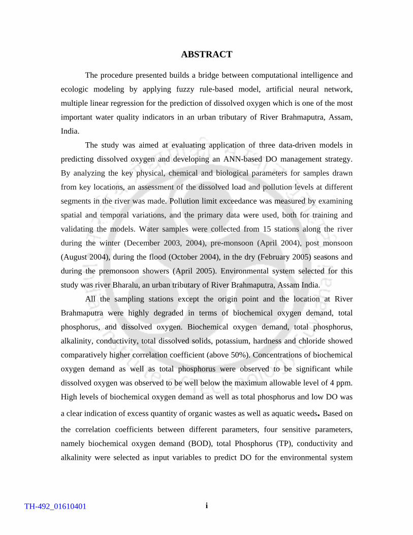
ABSTRACT

The procedure presented builds a bridge between computational intelligence and

ecologic modeling by applying fuzzy rule-based model, artificial neural network,

multiple linear regression for the prediction of dissolved oxygen which is one of the most

important water quality indicators in an urban tributary of River Brahmaputra, Assam,

India.

The study was aimed at evaluating application of three data-driven models in

predicting dissolved oxygen and developing an ANN-based DO management strategy.

By analyzing the key physical, chemical and biological parameters for samples drawn

from key locations, an assessment of the dissolved load and pollution levels at different

segments in the river was made. Pollution limit exceedance was measured by examining

spatial and temporal variations, and the primary data were used, both for training and

validating the models. Water samples were collected from 15 stations along the river

during the winter (December 2003, 2004), pre-monsoon (April 2004), post monsoon

(August 2004), during the flood (October 2004), in the dry (February 2005) seasons and

during the premonsoon showers (April 2005). Environmental system selected for this

study was river Bharalu, an urban tributary of River Brahmaputra, Assam India.

All the sampling stations except the origin point and the location at River

Brahmaputra were highly degraded in terms of biochemical oxygen demand, total

phosphorus, and dissolved oxygen. Biochemical oxygen demand, total phosphorus,

alkalinity, conductivity, total dissolved solids, potassium, hardness and chloride showed

comparatively higher correlation coefficient (above 50%). Concentrations of biochemical

oxygen demand as well as total phosphorus were observed to be significant while

dissolved oxygen was observed to be well below the maximum allowable level of 4 ppm.

High levels of biochemical oxygen demand as well as total phosphorus and low DO was

a clear indication of excess quantity of organic wastes as well as aquatic weeds. Based on

the correlation coefficients between different parameters, four sensitive parameters,

namely biochemical oxygen demand (BOD), total Phosphorus (TP), conductivity and

alkalinity were selected as input variables to predict DO for the environmental system

TH-492_01610401

ii

under study to develop a fuzzy rule based model and an artificial neural net work model.

A multiple linear regression model was also developed for comparison.

Out of the generated primary data sets 59 data sets were used for developing

fuzzy rule based model. A three- layer feed forward artificial neural network (ANN)

model having four input neurons, one output neuron and seven hidden neurons with

tansig and logsig as transfer functions gave satisfactory results in terms of root mean

square error and Nash efficiency. A multiple linear regression model was also developed

using the same input and output variables to have a comparison with the performance of

the best-fit ANN model. Of the three models developed ANN was observed to be the

best.

Sensitivity analysis was carried out with the best-fit simulated model using partial

derivative method to find the contribution of single variable as well as the interaction of

the variable. Interaction of variable is proved to have meaning than finding the

contribution of single variable for ecological modeling. Contour plots prepared using

parameters of the simulated neural network can successfully optimize the parameters for

the environmental system studied and can be used as an effective tool for the decision

makers to get an idea about combination of parameters, which can maintain the system

under study within the acceptable or the desirable level.

TH-492_01610401

iii

ACKNOWLEDGEMENTS

I would like to express my gratitude to all those who gave me the possibility to

complete this thesis. I want to thank the Department of Civil Engineering for giving me

permission to do the necessary research work

I am deeply indebted to my supervisor Dr.Chandan Mahanta for his continuous

support in the Ph.D program. His help, stimulating suggestions and encouragement

helped me in all the time of research and for writing of this thesis. He was always there to

meet and talk about my ideas, to proofread and mark up my papers and chapters, and to

ask me good questions to help me think through my problems.

A special thanks goes to Dr.Chandramouli who was my co-advisor during the

intial stage, for providing valuable insight as well for making me a better modeler and for

reviewing a part of this work.

Besides my advisors, I would like to thank the rest of my thesis committee

Dr.Talukdar, Prof.Arun Chatopadhyaya, Dr.Arup Sharma and Dr.Saswati Chakravarty

for their advice, suggestions and encouragement during the course of this research.

Let me also say ‘thank you’ to Mr.P.Pathak, (junior technician) of Dept of civil

engineering for lending a helping hand during my analysis in the lab. My heartful thanks

to Mr.Arun Borsokia, Jonali Saikia, Alok Mazumdar, Mrs. Juri Jyoti Hazarika and all

others for their timely help during the course of this work. I must thank all my fellow

research scholars for their lively discussions and cooperation.

I have to acknowledge and present my heartedly and highly appreciation to my

husband Prof.P.S.Robi for all the encouragement and support through out the tough time

that made the completion of this work possible. Special thanks to my daughters Parvathi

and Gayatri for their lovely spirits, which sweeps away my stress.

I feel a deep sense of gratitude for my late parents for educating me with aspects

from both arts and sciences, for unconditional support and encouragement to pursue my

interests. I am grateful to all my family members, for the encouragements and for

listening to my complaints and frustrations, and for believing in me.

Last but not least, thanks be to God for my life through all tests in the past years.

You have made my life more bountiful.

TH-492_01610401

iv

CONTENTS

ABSTRACT . . . . . . . . . . . . . . . . . . . . . . . . . . . . . . . . . . . . . . . . . . . . . . . . . . . . . . . . . . . i

ACKNOWLEDGEMENTS . . . . . . . . . . . . . . . . . . . . . . . . . . . . . . . . . . . . . . . . . . . . . . . iii

LIST OF TABLES . . . . . . . . . . . . . . . . . . . . . . . . . . . . . . . . . . . . . . . . . . . . . . . . . . . . viii

LIST OF FIGURES . . . . . . . . . . . . . . . . . . . . . . . . . . . . . . . . . . . . . . . . . . . . . . . . . . . . ix

LIST OF NOTATIONS . . . . . . . . . . . . . . . . . . . . . . . . . . . . . . . . . . . . . . . . . . . . . . . . . .xii

LIST OF ABBREVIATIONS . . . . . . . . . . . . . . . . . . . . . . . . . . . . . . . . . . . . . . . . . . . .xiii

CHAPTER 1 INTRODUCTION . . . . . . . . . . . . . . . . . . . . . . . . . . . . . . . . . . . . . 1

1.1 THE CONTEXT . . . . . . . . . . . . . . . . . . . . . . . . . . . . . . . . . . . . . . . . . . . . . . . . . . 1 1.2 NEED FOR MODELING . . . . . . . . . . . . . . . . . . . . . . . . . . . . . . . . . . . . . . . . . . . 1

1.3 DATA DRIVEN MODELS . . . . . . . . . . . . . . . . . . . . . . . . . . . . . . . . . . . . . . . . . . 2

1.3.1 Rule based models. . . . . . . . . . . . . . . . . . . . . . . . . . . . . . . . . . . . . . . . . . . . .2

1.3.2 Artificial neural network model . . . . . . . . . . . . . . . . . . . . . . . . . . . . . . . . . . 2

1.3.3 Multiple linear regression model . . . . . . . . . . . . . . . . . . . . . . . . . . . . . . . . . .3

1.4 THE PRESENT STUDY . . . . . . . . . . . . . . . . . . . . . . . . . . . . . . . . . . . . . . . . . . . . 3

1.5 OBJECTIVES OF THE PRESENT STUDY . . . . . . . . . . . . . . . . . . . . . . . . . . . . .3

1.6 THE APPROACH . . . . . . . . . . . . . . . . . . . . . . . . . . . . . . . . . . . . . . . . . . . . . . . . .4

CHAPTER 2 LITERATURE REVIEW . . . . . . . . . . . . . . . . . . . . . . . . . . . . . . . . . . . . 7

2.1 INTROUCTION . . . . . . . . . . . . . . . . . . . . . . . . . . . . . . . . . . . . . . . . . . . . . . .7

2.2 STUDIES ON WATER QUALITY ASSESSMENT. . . . . . . . . . . . . . . . . . . . . . . 7

2.3.ECOLOGICAL MODELING . . . . . . . . . . . . . . . . . . . . . . . . . . . . . . . . . . . . . . . .12

2.3.1 Mathematical models . . . . . . . . . . . . . . . . . . . . . . . . . . . . . . . . . . . . . . . . 12

2.3.2.Fuzzy models . . . . . . . . . . . . . . . . . . . . . . . . . . . . . . . . . . . . . . . . . . . . . . . .14

2.3.3 Artificial neural network models . . . . . . . . . . . . . . . . . . . . . . . . . . . . . . . . .26

2.4 PARAMETRIC STUDIES . . . . . . . . . . . . . . . . . . . . . . . . . . . . . . . . . . . . . . . . . .42 2.5 CONCLUSIONS . . . . . . . . . . . . . . . . . . . . . . . . . . . . . . . . . . . . . . . . . . . . . . . . . 43

CHAPTER 3 WATER QUALITY ANALYSIS AND LAND USE

CLASSIFICATION . . . . . . . . . . . . . . . . . . . . . . . . . . . . . . . . . . . . . . . 44

TH-492_01610401

v

3.1 THE ENVIRONMENTAL SYSTEM CONSIDERED FOR THE STUDY . . . . 44

3.2 MATERIALS AND METHODS . . . . . . . . . . . . . . . . . . . . . . . . . . . . . . . . . . . . 46

3.2.1 Analytical methods and instruments . . . . . . . . . . . . . . . . . . . . . . . . . . . . . . 47

3.2.2 Recommended water quality criteria . . . . . . . . . . . . . . . . . . . . . . . . . . . . . .47 3.2.3 Calculation of correlation coefficient . . . . . . . . . . . . . . . . . . . . . . . . . . . . . 48 3.3 LAND USE CLASSIFICATION . . . . . . . . . . . . . . . . . . . . . . . . . . . . . . . . . . . . 49

3.3.1 Geometric correction . . . . . . . . . . . . . . . . . . . . . . . . . . . . . . . . . . . . . . . . . 50

3.3.2 Image enhancement . . . . . . . . . . . . . . . . . . . . . . . . . . . . . . . . . . . . . . . . . . 50

3.3.3 Image classification . . . . . . . . . . . . . . . . . . . . . . . . . . . . . . . . . . . . . . . . . . .50

3.3.4 Field verification . . . . . . . . . . . . . . . . . . . . . . . . . . . . . . . . . . . . . . . . . . . . . 51

3.3.5 GIS model developed. . . . . . . . . . . . . . . . . . . . . . . . . . . . . . . . . . . . . . . . . . 51

3.4 SUMMARY . . . . . . . . . . . . . . . . . . . . . . . . . . . . . . . . . . . . . . . . . . . . . . . . . . . . .51

CHAPTER 4 RESULTS AND DISCUSSION ON WATER

QUALITY ANALYSIS . . . . . . . . . . . . . . . . . . . . . . . . . . . . . . . . . . . . . .54

4.1 WATER QUALITY ANALYSIS . . . . . . . . . . . . . . . . . . . . . . . . . . . . . . . . . . . . .54

4.2 DESCRIPTION OF THE MOST POLLUTED STATION . . . . . . . . . . . . . .. . 88

4.3 CORRELATION COEFFICIENTS OF PARAMETERS . . . . . . . . . . . . . . . . . 89

4.3.1 Correlation matrix . . . . . . . . . . . . . . . . . . . . . . . . . . . . . . . . . . . . . . . . . . . 89

4.4 CONCLUSION . . . . . . . . . . . . . . . . . . . . . . . . . . . . . . . . . . . . . . . . . . . . . . . . . . 94

CHAPTER 5 MODELING METHODOLOGY . . . . . . . . . . . . . . . . . . . . . . . . . . . 96 5.1 INPUTS AND OUTPUT VARIABLE . . . . . . . . . . . . . . . . . . . . . . . . . . . . . . . . 96

5.2 FUZZY RULE BASED MODEL . . . . . . . . . . . . . . . . . . . . . . . . . . . . . . . . . . . . 97

5.2.1 Description of fuzzy regions . . . . . . . . . . . . . . . . . . . . . . . . . . . . . . . . . . . 98

Fuzzy subsets for BOD ………………………. . . . . . . . . . . . . .100

Fuzzy subsets for total phosphorus . . . . . . . . . . . . . . . . . . . . . . .102

Fuzzy subsets for conductivity . . . . . . . . . . . . . . . . . . . . . . . . . . 104

Fuzzy subsets for alkalinity . . . . . . . . . . . . . . . . . . . . . . . . . . . . 106

Fuzzy subsets for dissolved oxygen . . . . . . . . . . . . . . . . . . . . . 108

5.2.2 Defuzzification . . . . . . . . . . . . . . . . . . . . . . . . . . . . . . . . . . . . . . . . . . . . . 113

5.2.3 Performance of the model . . . . . . . . . . . . . . . . . . . . . . . . . . . . . . . . . . . 113

5.3 ARTIFICIAL NEURAL NETWORK MODEL . . . . . . . . . . . . . . . . . . . . . . . . 114

TH-492_01610401

vi

5.3.1 Data normalization . . . . . . . . . . . . . . . . . . . . . . . . . . . . . . . . . . . . . . . . . . .114

5.3.2 Training algirithm used . . . . . . . . . . . . . . . . . . . . . . . . . . . . . . . . . . . . . . . 115

5.3.3 Generalization. . . . . . . . . . . . . . . . . . . . . . . . . . . . . . . . . . . . . . . . . . . . . . .116

5.4 MULTIPLE LINEAR REGRESSION MODEL . . . . . . . . . . . . . . . . . . . . . . . . 118

5.5 USE OF ANN FOR PARAMETRIC STUDIES . . . . . . . . . . . . . . . . . . . . . . . . 119

5.5.1 Assessment of contribution of input variables . . . . . . . . . . . . . . . . . . . . . .119

5.5.2 Variable optimization using contour plots . . . . . . . . . . . . . . . . . . . . . . . . .121

5.6 SUMMARY . . . . . . . . . . . . . . . . . . . . . . . . . . . . . . . . . . . . . . . . . . . . . . . . . . . .122

CHAPTER 6 PERFOMANCE STUDIES OF THE MODELS AND

PARAMETRIC STUDIES . . . . . . . . . . . . . . . . . . . . . . . . . . . . . . . . . .123

6.1 RESULTS OF FUZZY RULE BASED MODELING . . . . . . . . . . . . . . . . . . . .123

6.1.1 Conclusions. . . . . . . . . . . . . . . . . . . . . . . . . . . . . . . . . . . . . . . . . . . . . . . . .128

6.2 ARTIFICIAL NEURAL NETWORK MODEL PERFORMANCE . . . . . . . . . 129

6.3 DO PREDICTION USING MULTIPLE LINEAR REGRESSION MODEL . .131

6.4 CONCLUSIONS ON MODEL PERFORMANCE . . . . . . . . . . . . . . . . . . . . . 136

6.5 CONRIBUTION OF VARIABLES USING SIMULATED NEURAL

NETWORK . . . . . . . . . . . . . . . . . . . . . . . . . . . . . . . . . . . . . . . . . . . . . . . . . . . . 138

6.5.1 Conclusions . . . . . . . . . . . . . . . . . . . . . . . . . . . . . . . . . . . . . . . . . . . . . . . .144 6.6 OPTIMIZATION OF VARIABLES USING CONTOUR PLOTS . . . . . . . . . .144

6.6.1 Comparison of inference of the contour plots with

experimental data . . . . . . . . . . . . . . . . . . . . . . . . . . . . . . . . . . . . . . . . . . . 150

6.6.2 Conclusions on contour plots. . . . . . . . . . . . . . . . . . . . . . . . . . . . . . . . . . . 163

CHAPTER 7 MAJOR CONCLUSIONS . . . . . . . . . . . . . . . . . . . . . . . . . . . . . . . . . 164

SCOPE FOR FUTURE RESEARCH . . . . . . . . . . . . . . . . . . . . . . . . . . . . . . . . . . . . .166

REFERENCES . . . . . . . . . . . . . . . . . . . . . . . . . . . . . . . . . . . . . . . . . . . . . . . . . . . . . . 167

LIST OF PUBLICATIONS . . . . . . . . . . . . . . . . . . . . . . . . . . . . . . . . . . . . . . . . . . . . .176

TH-492_01610401

vii

LIST OF TABLES

Table 3.1 Description of sampling locations . . . . . . . . . . . . . . . . . . . . . . . . . . . . . . . . . 46

Table 3.2 Acceptable levels of surface water pollutants . . . . . . . . . . . . . . . . . . . . . . . . .49

Table 3.3 Details of catchment area of sampling points from GIS model and remote

sensing area . . . . . . . . . . . . . . . . . . . . . . . . . . . . . . . . . . . . . . . . . . . . . . . . . . . 53

Table 4.1 Correlation matrix generated from the analysis results . . . . . . . . . . . . . . . . 90

Table 5.1 Input (P) and output (T) parameters for modeling . . . . . . . . . . . . . . . . . . . . 97

Table 5.2 Description of fuzzy sets for BOD . . . . . . . . . . . . . . . . . . . . . . . . . . . . . . . .100

Table 5.3 Description of fuzzy sets for TP . . . . . . . . . . . . . . . . . . . . . . . . . . . . . . . . . . 102

Table 5.4 Description of fuzzy sets for conductivity . . . . . . . . . . . . . . . . . . . . . . . . . . .104

Table 5.5 Description of fuzzy sets for alkalinity . . . . . . . . . . . . . . . . . . . . . . . . . . . . . 106

Table 5.6 Descriptions of fuzzy sets for dissolved oxygen . . . . . . . . . . . . . . . . . . . . . 108

Table 5.7 Fuzzy rule base based on experimental data . . . . . . . . . . . . . . . . . . . . . . . . 111

Table 6.1 Inferences from the contour plots . . . . . . . . . . . . . . . . . . . . . . . . . . . . . . . . .150

Table 6.2 Data sets with DO above 6 mg/L . . . . . . . . . . . . . . . . . . . . . . . . . . . . . . . . . 151

Table 6.3 Comparisons of the original data with results from contour plots . . . . . . . . 163

TH-492_01610401

viii

LIST OF FIGURES

Figure 1 Environmental system selected for the study . . . . . . . . . . . . . . . . . . . . . . . .6

Figure 3.1. Guwahati city drainage . . . . . . . . . . . . . . . . . . . . . . . . . . . . . . . . . . . . . . . . .45

Figure 3.2 Land use pattern map. . . . . . . . . . . . . . . . . . . . . . . . . . . . . . . . . . . . . . . . . . .52

Figure 4.1 Pollution level of location 1 based on the standardized value of the

concentration of parameters . . . . . . . . . . . . . . . . . . . . . . . . . . . . . . . . . . . . . 55




concentartion of parameters . . . . . . . . . . . . . . . . . . . . . . . . . . . . . . . . . . . . . .60

Figure 4.4 Pollution level of location 4a based on the standardized value of the

concentration of parameters . . . . . . . . . . . . . . . . . . . . . . . . . . . . . . . . . . . . . .63

Figure 4.5 Pollution level of location 4b based on the standardized value of the


Figure 4.6 Pollution level of location 4m based on the standardized value of the






Figure 4.9 Pollution level of location 7a based on the standardized value of the


Figure 4.10 Pollution level of location 7b based on the standardized value of the

concentration of parameters . . . . . . . . . . . . . . . . . . . . . . . . . . . . . . . . . . . . .77

Figure 4.11 Pollution level of location 7m based on the standardized value of the

concentration of parameters . . . . . . . . . . . . . . . . . . . . . . . . . . . . . . . . . . . . 79





TH-492_01610401

ix





Figure 4.16 Variation of DO with respect to tp and bod . . . . . . . . . . . . . . . . . . . . . . . . 89

Figure 4.17 Correlation coefficients of parameters with respect to dissolved oxygen . .91

Figure 4.18 Average values of parameters having correlation coefficient above 50% . 93

Figure 5.1 Fuzzy subsets for BOD based on concentration. . . . . . . . . . . . . . . . . . . . .101

Figure 5.2 Fuzzy subsets for total phosphorus based on concentration. . . . . . . . . . . .103

Figure 5.3 Fuzzy subsets for conductivity based on concentration. . . . . . . . . . . . . . ..105

Figure 5.4 Fuzzy subsets for alkalinity based on concentration. . . . . . . . . . . . . . . . . . 107

Figure 5.5 Fuzzy subsets for DO based on concentration. . . . . . . . . . . . . . . . . . . . . . .109

Figure 5.6 Fuzzy system with 4 inputs and 1 input used in the study . . . . . . . . . . . . . 110

Figure 5.7 Neural network topology used in the study . . . . . . . . . . . . . . . . . . . . . . . . 117

Figure 6.1 Results of fuzzy model for training data . . . . . . . . . . . . . . . . . . . . . . . . . . .124

Figure 6.2 Performance of fuzzy model for training data . . . . . . . . . . . . . . . . . . . . . . 125

Figure 6.3 Results of fuzzy model for validation data . . . . . . . . . . . . . . . . . . . . . . . . . 126

Figure 6.4 Performance of fuzzy model for validation data . . . . . . . . . . . . . . . . . . . . .127

Figure 6.5 Plot of rmse against hidden layer neurons . . . . . . . . . . . . . . . . . . . . . . . . . 130

Figure 6.6 Results of MLR using simple linear equation . . . . . . . . . . . . . . . . . . . . . . .132

Figure 6.7 Results of (i) ANN and (ii) MLR simulations for training data . . . . . . . . 133

Figure 6.8 Results of (i) ANN and (ii) MLR simulations for testing data . . . . . . . .134

Figure 6.9 Results of (i) ANN and (ii) MLR simulations for validation data . . . . . . .135

Figure 6.10 Comparison of ANN and MLR results . . . . . . . . . . . . . . . . . . . . . . . . . . . 137

Figure 6.11 Partial derivatives of the ANN model response (DO) with respect to each

independent variable . . . . . . . . . . . . . . . . . . . . . . . . . . . . . . . . . . . . . . . . . . 139

Figure 6.12 Results of partial derivative method showing

relative contribution of each input variable . . . . . . . . . . . . . . . . . . . . . . . . .140

Figure 6.13 Partial deriative of DO-3D graph for two way

interaction . . . . . . . . . . . . . . . . . . . . . . . . . . . . . . . . . . . . . . . . . . . . . . . . . . 142

Figure 6.14 Results of PaD method for two-way interaction . . . . . . . . . . . . . . . . . . . . .143

TH-492_01610401

x

Figure 6.15 Contour plots for DO concentration vs TP &

BOD, when conductivity =50 µS/cm, alkalinity = 25 mg/L . . . . . . . . . . . .146

Figure 6.16 Contour plots for DO concentration vs TP &

BOD, when conductivity = 300 µS/cm, alkalinity = 150 mg/L . . . . . . . . .146

Figure 6.17 Contour plots for DO concentration vs

conductivity & alkalinity, when BOD = 0 mg/L, TP = 0.03 mg/L . . . . . . .147


conductivity & alkalinity, when BOD = 10 mg/L & TP = 1 mg/L . . . . . . 147


conductivity & BOD, when alkalinity = 25 mg/L, TP = 0.04 mg/L . . . . . .148


conductivity & BOD,when alkalinity = 180 mg/L, TP = 1 mg/L. . . . . . . .148


conductivity &TP, when BOD = 0 mg/L, alkalinity = 25 mg/L . . . . . . . . 149


conductivity & TP, when BOD = 8 mg/L, alkalinity = 200 mg/L . . . . . . .149

Figure 6.23 Contour plots for DO concentration vs BOD & TP, when

conductivity = 80 µ S/cm, alkalinity = 80 ppm . . . . . . . . . . . . . . . . . . . . . 152


conductivity &alkalinity, when BOD = 6 ppm & TP = 0.5 mg/L . . . . . . . 153

Figure 6.25 Contour plots for DO concentration vs BOD & TP, when

conductivity = 175 µS/cm, alkalinity = 150 mg/L . . . . . . . . . . . . . . . . . . . .154

Figure 6.26 Contour plots for do concentration vs

conductivity &alkalinity, when BOD = 1 mg/L, TP = 0.2 mg/L . . . . . . . .155


conductivity &alkalinity, when BOD = 0.2 mg/L, TP = 0.6 mg/L . . . . . . 156

Figure 6.28 Contour plots for DO concentration vs BOD &TP, when

conductivity = 80 µS/cm, alkalinity = 30 mg/L . . . . . . . . . . . . . . . . . . . . . 157

Figure 6.29 Contour plots for DO concentration vs TP & BOD,when

conductivity = 50 µS/cm, alkalinity = 30 mg/L . . . . . . . . . . . . . . . . . . . . . .158

Figure 6.30 Contour plots for DO concentration vs TP &BOD, when

TH-492_01610401

xi

conductivity = 175 µS/cm, alkalinity = 75 mg/L . . . . . . . . . . . . . . . . . . . . 159

Figure 6.31 Contour plots of DO vs conductivity & alkalinity, when

BOD = 3 mg/L, TP = 0.5 mg/L . . . . . . . . . . . . . . . . . . . . . . . . . . . . . . . . . .160

Figure 6.32 Contour plots of DO vs TP & alkalinity, when

conductivity = 260 µS/cm, alkalinity = 100 mg/L . . . . . . . . . . . . . . . . . . .161

Figure 6.33 Contour plots of DO vs conductivity & alkalinity, when

BOD = 3 mg/L, TP = 0.9 mg/ L . . . . . . . . . . . . . . . . . . . . . . . . . . . . . . . . . 162

TH-492_01610401

xii

NOTATIONS

b1 Bias matrix connecting input layer and hidden layer

b2 Bias matrix connecting hidden layer and output layer

Dj Derivative of output with respect to its input

dji Partial derivative of ith input of jth observation

K Regression coefficient

µ Membership function

nPi Normalized value of ith input variable

nt Normalized value of output variable

Pi Input value of ith data set

Pmax Maximum value of input variable

Pmin Minimum value of input variable

r Correlation coefficient

R2 Coefficient of determination

RMSE Root mean square error value

SSDi Sum of the squared partial derivative for ith

input

ti Output value of the ith data set

W1 Weight matrix connecting the input layer and the hidden layer

W2 Weight matrix connecting the hidden layer and the output layer

TH-492_01610401

xiii

ABBREVIATIONS

ANN Artificial neural network

GIS Geographical Information System

BIS Bureau of Indian Standards

BOD Biochemical oxygen demand

COA Center of area

COG Center of gravity

COS Center of sums

DO Dissolved oxygen

EDTA Ethylene diamine tetra acetic acid

LOGSIG Logarithmic sigmoid function

MLR Multiple linear regression model

MOM Means of maxima

PaD Partial derivative

SVM Support vector machine TDS Total dissolved solids

TI Total iron

TP Total phosphorus

TS Total solids

TANSIG Tangent sigmoid function

USPH United States public health

WHO World health organization

TH-492_01610401

111

CHAPTER ONE INTRODUCTION

1.1 THE CONTEXT

The growing problem of degradation of our river ecosystems has necessitated

the monitoring of water quality of various rivers to evaluate their primary production

capacity, utility potential and to plan restorative measures. As opined by Gorchev,

(1996), in the third world countries, 80% of all diseases are directly related to poor

drinking water and unsanitary conditions. The industrial units located at the outskirts

of cities, intensive agricultural practices, and indiscriminate disposal of domestic and

municipal wastes are the sources of contamination for the river water and

groundwater. Thus, constant monitoring of river water and groundwater quality is

needed so as to record any alteration in the quality and outbreak of health disorders as

well as for water quality management (Olajire & Imeokaparia, 2001). Because of the

complexity of environmental data sets, in particular, with regard to the ecosystem functioning, decision makers need reliable support on the effects of the management

options they eventually consider.

1.2 NEED FOR MODELING

Prediction models are considered useful for river basin management and are

used to predict behaviour of water quality with respect to changes in pollution loads

and hydrological conditions. Models allow us to simulate changes in our ecosystem

due to changes in population, land use or pollution management. These simulations

allow us to predict changes, negative or positive, within our ecosystem due to

management actions such as improved sewage treatment, reduced fertilizer or manure

application on agricultural land, or controlling urban growth. In order to maintain

water quality with in the standards, various computational tools are being used.

Ecosystem management combines the structuring and understanding of ecological

information to facilitate the decision making in order to meet the society goals. Water

quality predictive models include both mathematical expressions and expert scientific

judgement. They include process-based models and data based models. Modeling is

TH-492_01610401

222

the linkage between pollution source and the instream water quality of a given water

body.

1.3 DATA DRIVEN MODELS

Models used in ecosystem management have to deal with a large number of

uncertainties exist due to the complex physical and biochemical processes involved in

these systems. Traditional modeling of physical processes is often named physically

based modeling (or knowledge based modeling) because it tries to explain underlying

processes. Those models require preparation of extensive input data sets and a time

consuming calibration and verification process that is often too expensive for small

utilities and municipalities. On the contrary, the so called data driven models borrow

heavily from artificial intelligence techniques are based on a limited knowledge of the

modeling process and rely on the data describing input and output characteristics.

Hence such models are suited for modeling ecosystems to deal with uncertainties

arising out of limitation of knowledge of underlying processes. The predictive

methods used for forecasting different environmental variables employs connectionist

method like neural networks, SVMs, fuzzy rule based systems etc.

1.3.1.RULE BASED MODELS

Rule-based models often deal with the linguistic aspect. The linguistic aspect

could be based on two different approaches in ecosystem management: (1) expert

knowledge and/or ecological (monitoring) data are available in a linguistic format and

because of the imprecision of the natural language, we are dealing with linguistic

uncertainty; (2) ecosystem managers want the models developed for decision support

to be interpretable and transparent. Rule based models can also work with epistemic

uncertainty, integrating imprecision and variability inherent to ecological data.

(Adriaenssens et al., 2004). Because of these aspects, approaching ecosystem

management by reasoning according to the principles of ‘fuzzy logic’, in particular by

means of fuzzy-rule based models, are found to be appropriate. 1.3.2.ARTIFICIAL NEURAL NETWORK MODEL

The use of ANN is particularly useful when the physical world is not fully

defined, when the model has many uncertainties in terms of model coefficients and/or

TH-492_01610401

333

input parameters, and when there is extensive data for training the network. This is

essentially a non-linear `black-box' approach, which assumes a set of prescribed

intermediate relations that enables the output(s) to be predicted from a number of

input parameters. The parameters of these relations (the network) can be obtained by

`training' the network using past data; the success of the prediction is then tested

against future data or known data sets that were not used in the training set.

1.3.3.MULTIPLE LINEAR REGRESSION MODEL

Linear regression model is a simple example of a data driven model.

Coefficients of the regression equation are trained on the basis of the available

existing data and then for a new value of independent (input) variable it gives an

approximation of an output variable value. When it is required to model the

relationship between two or more explanatory variables and a response variable

multiple liner regression is used. Every value of the independent variable x is

associated with a dependant variable y.

1.4 THE PRESENT STUDY

In the present study, water quality analysis of river Bharalu, a tributary of the

river Brahmaputra in Assam, was carried out for modeling and prediction. After

careful consideration of the possible attributes, parameters analyzed were pH,

dissolved oxygen, biochemical oxygen demand, hardness, alkalinity, total dissolved

solids, total solids, chloride, total phosphorus, total iron, sodium, potassium, and

calcium. Based on the analysis results, assessment of the dissolved load and pollution

levels at different segments of the river was made and pollution limit exceedance was

measured by examining spatial and temporal variations. All these parameters were

found to influence the water quality to different degree, and the data generated was

used for training, and validating the models. Enironmental system selected for the

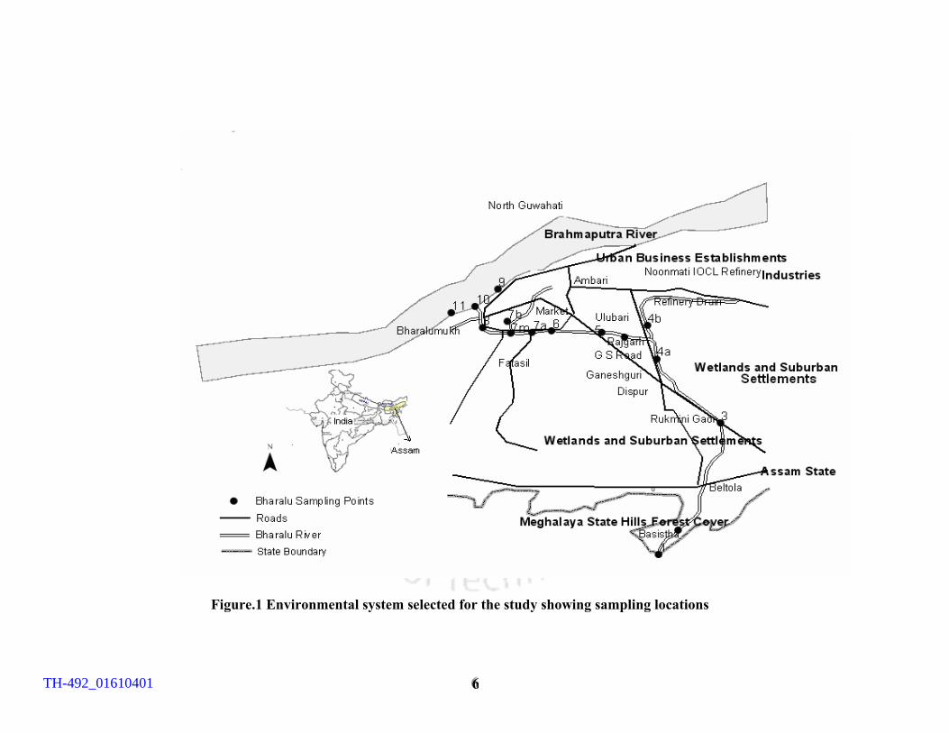
study and of the sampling locations is shown in Figure 1.

1.5 OBJECTIVES OF THE PRESENT STUDY

Dissolved oxygen is only one of the vital characteristics of an open

watercourse and it has traditionally been used as a variable of water quality. This

selection is based on the relationship observed between its concentration decrease and

its non-desirable effects on the water column. If the dissolved oxygen concentration

TH-492_01610401

444

in a particular environmental system could be predicted only from data that are

collected in real time, then river managers would be better able to manage the river’s

water quality. The river’s dissolved oxygen is influenced greatly by physical and

meteorological factors, but whether the concentration of dissolved oxygen

concentration can be predicted from such factors with any accuracy was unknown.

The purpose of this study was to determine the extent to which the dissolved oxygen

concentration in the Bharalu river can be predicted solely from, the selected sensitive

parameters that are having comparatively higher correlation with dissolved oxygen

using fuzzy rule base, multiple linear regression and artificial neural network

modeling techniques and to have a comparison among different methods. Sensitivity

analysis was carried out for evaluating the contribution of single input as well two-

way interaction by using partial derivative method and the most influencing input

variable and the pair of variables were identified. Contour plots were drawn keeping

the values of two parameters fixed and giving increments to the other two parameters.

This enables the decision makers to decide on which parameter level should be

controlled and to what extend.

1.6 THE APPROACH

Rigorous laboratory analysis of samples was carried out to find the seasonal

variation of the water quality of River Bharalu. Three data driven models namely the

fuzzy rule based model, artificial neural network, and multiple linear regression were

developed and their performance were studied and compared. Parametric studies were

carried out with the best-fit simulated model to assess the contribution of each

variable as well as by interaction and to investigate optimized region of the variables

to be maintained for the environmental system under study with good ecological

status.

A thorough literature review was undertaken that covered studies on water

quality monitoring, analysis and use of different ecological models for water quality

prediction. This review is reported in Chapter 2. Methodology adopted to carry out

the analysis of water samples, documenting the results and land use characteristics of

the system studied are explained in chapter 3. Results and interpretation of analysis of

the water samples are detailed in chapter 4. The approaches selected for the three data

TH-492_01610401

555

driven models viz, fuzzy rule based model, artificial neural network model and the

multiple linear regression model and parametric studies are presented in chapter 5.

Chapter 6 deals with the performance of the models studied and interpretation of the

results. Finally major conclusions of the study are presented in chapter 7.

TH-492_01610401

666

Figure.1 Environmental system selected for the study showing sampling locations

TH-492_01610401

777

CHAPTER TWO

LITERATURE REVIEW

2.1 INTROUCTION

Environmental pollution, mainly of water resources, has become of public

interest. Not only the developed countries have been affected by environmental

problems, but also the developing nations suffer the impact of pollution, due to

disordered economic growth associated with the exploration of virgin natural

resources (Gibbs, 1972). Dissolved oxygen is an important indicator describing the

general health of water bodies, and it can be used to estimate community metabolism

of a stream in terms of gross photosynthesis and respiration rates. Different land use

may alter the relative importance of photosynthesis and respiration in streams.

Fluctuation of DO near saturation, with diurnal variation due to temperature and

metabolism, implies relatively healthy waters. A marked depression of DO below

saturation indicates the stream receiving untreated wastewater or an excessive amount

of nutrients from non-point source pollution (Wilcock, 1986, Wang et al., 2003).

2.2 STUDIES ON WATER QUALITY ASSESSMENT\

Investigation on New Zealand’s surface water quality by Smith and Maasdam,

1994 revealed that vast majority samples were within the acceptable standards and

criteria for a variety of river water uses and the waters can be classed as being of

relatively low ionic strength. Relatively high conductance in very few locations,

which was due to the geo thermal, input of high BOD5 in one location as a

consequence of industrial wastewater discharge was observed.

Water quality and reaeration aspects of Whangamaire stream (North Island,

New Zealand) were studied by Wilcock et al., (1995) to explain the observed DO

levels. Studies showed that respiration was dominant in the lower reach where

photosynthetic activity was inhibited by shade. It was opined in the study that better

riparian management and reduced nutrient inputs are likely to improve stream water

quality.

TH-492_01610401

888

Studies conducted on Epic creek which is a distributary of the Nun River the

in Niger delta by Izonfuo and Bariweni, (2001) recommended proper management of

wastes and controlling and monitoring of other human activities to ensure that the

runoff would have a minimum effect on the creek. Concentrations of chloride,

sulphate, phosphate, nitrate and ammonia were found to increase during the rainy

season, which means that runoff water contributes a significant proportion of these

constituents into the Epic creek. Human activities were found to be the cause of

higher levels of several parameters in the creek than that in the upstream.

Silva and Sacomani, (2001) carried out a study to determine the water quality

in the Pardo River located in Botucatu region in Brazil, with certain chemical

physical indicators, coliforms and chemical species of samples taken monthly.

Principal component analysis (PCA) was applied to normalize data to assess

association between variables and has achieved meaningful classification of hydro

chemical variables and of river water samples based on seasonal and spatial criteria.

The application of multivariate statistical techniques to the data collected in this study

showed that the Pardo River water quality is changed because it received water with

high salt content causing damage and degradation. Diffuse pollution was identified as

a cause of water quality degradation in the Pardo River. Other parameters, such as

geology, land use, topography, storm flow, weather, etc., can control or increase the

amount of nutrients released by the drainage basin throughout the length of the Pardo

River.

Patterns of historical watershed nutrient inputs were compared by Stow et al.,

(2001) with in-river nutrient loads for the Neuse River. Studies showed that there was

a substantial increase in the nitrogen and phosphorus inputs as a result of intensified

animal production, but this increase was not reflected in changes in river loadings. It

was concluded that it could be due to the terrestrial storage in ground water or

riparian zones preventing or slowing the transport of nutrients from an on-land source

to the river channel or denitrification and volatilization in agricultural and riparian

soils that remove nitrogen from watershed before it enters the river. Smith, (2001) presented a case study of storm water and sediment analysis for

conventional pollutants in flood control sumps of the city of Dallas, along the Trinity

TH-492_01610401

999

River, which is channelized and leveed through most of the city. Pollutant analysis at

both pumping station and sump outfall suggested that rigorous sampling is needed to

obtain reliable results and collection of storm water samples in the vicinity of the

sump pumping station and selected outfalls as a function of time would enable

estimation of pollutant loads to and discharged from the sump, and estimation of

pollutant removal in the sump by settling and other physical- chemical processes.

Study on pollution assessment in the Keiskamma River and in the

impoundment downstream was carried out by Fatoki et al., (2003) over a one-year

period by using standard physico chemical method. Significant pollution of the river

and the impoundment from the Keiskammahoek Sewage Treatment Plant (KSTP)

was indicated for electrical conductivity, nutrients and oxygen-demanding substances.

The use of the WQI (water quality index) and the dissolved oxygen deficit

(D) as simple indicators of a watershed pollution was investigated and compared in

the Municipality of Las Rozas (north-west of Madrid, Spain) by Sanchez et al.,

(2006). The quality of the water in Guadarrama and Manzanares rivers and Paris Park

ponds, the main watersheds of this area was investigated during 2 years (from

September 2001 to September 2003). The monitoring of the Las Rozas watersheds

demonstrated that water quality of Guadarrama watershed was slightly affected in the

section of the river within this town. It was found that the WQI was very useful for

the classification of the waters monitored. A high linear relationship between the

WQI and the oxygen deficit (D) of the samples was found. The classifications of

water based on the two methods coincided in 93% of the samples studied. This

allowed the determination of WQI based on the values of the oxygen deficit. It was

found that water quality was influenced by the climatic conditions, the highest

qualities being observed during the winter.

A study was carried out by Woli et al., (2004) to evaluate the quality of river

water by analysis of land use in drainage basins and by estimating the N budgets in

the drainage basins of Shibetsu River (Shibetsu area) and Bekkanbeushi River

(Akkeshi area) in eastern Hokkaido, Japan. The evaluation of water quality was up-

scaled to the regional level in Hokkaido by using the Arcviewy GIS and statistical

information. The linear regression results showed that the correlation between NO –N

TH-492_01610401

111000

concentration and the proportion of upland in the drainage basins was highly and

positively significant for both the areas. Study results indicated that the impact factors

were highest for intensive livestock farming areas; medium for mixed agriculture and

livestock farming, and the lowest for grassland-based dairy cattle and horse farming

areas. The results of a simple regression analysis showed that the impact factors had a

significant positive correlation with the cropland surplus N (r=0.93, P<0.01),

chemical fertilizer N (r=0.82, P<0.05), and manure fertilizer N (r=0.76, P<0.05),

which were estimated by using the N budget approach. Using the best-correlated

regression model, impact factors for all cities, towns and villages of the Hokkaido

region were estimated. The regression analysis indicated that the predicted NO–N

concentrations were significantly correlated (r=0.62, P<0.001, n=203) with the

measured NO –N concentrations, reported previously. It was concluded that by

estimating the proportions of upland fields in drainage basins, and calculating

cropland surplus N it is possible to predict river water quality with respect to NO–N

concentration.

The application of a battery of toxicity and genotoxicity tests on pore water in

parallel and in combination with physico-chemical analyses and benthic macro

invertebrate community investigations is discussed by Isidori et al,(2004) to assess

the environmental quality of the Volturno River in South Italy. Toxicity testing was

performed on the rotifer Brachionus calyciflorus and the crustacean Daphnia magna.

Genotoxicity was determined by the SOS chromotest and Mutatox system. The

physico-chemical characterization of the surface waters showed a declining trend

from up-river to down-river for dissolved oxygen and conductivity. Also, chemical

variables showed a worsening along the river axis showing an increase in ammonium,

phosphates, sulfates, and heavy metals. The assessment of macro invertebrates

reflected the general ecological deterioration occurring to chemical as well as toxic

and genotoxic pollution. A strong correlation was observed between the benthic

community composition and the sediment contamination of toxic and genotoxic

substances.

Taebi and Droste, (2004) conducted an analysis to investigate the pollution

loads in urban runoff compared to point source loads as a first prerequisite for

TH-492_01610401

111111

planning and management of receiving water quality. Unit loads were estimated in

storm water runoff, raw sanitary wastewater and secondary treatment effluents in

Isfahan, Iran. Results indicated that the annual pollution load in urban runoff is lower

than the annual pollution load in sanitary wastewater in areas with low precipitation

but it is higher in areas with high precipitation. Two options, namely, advanced

treatment (in lieu of secondary treatment) of sanitary wastewater and urban runoff

quality control systems (such as detention ponds) were investigated as controlling systems for pollution discharges into receiving waters. The results revealed that for

Isfahan, as a low precipitation urban area, advanced treatment is a more suitable

option, but for high precipitation urban areas, urban surface runoff quality control

installations were more effective for suspended solids and oxygen-demanding matter

controls, and that advanced treatment is the more effective option for nutrient control.

Judova and Jansky, (2005) evaluated the water quality in rural areas in the

Czech part of Labe River catchment using the example of Slapanka River catchment.

This river drains a typical landscape of Ceskomoravska Highland. It was observed that agriculture and production of municipal wastewater resulting in increased

eutrophication caused increased amount of organic substances and nutrients.

Identifying the type of the pollution source is helped by regression analysis using data

from the public monitoring network. Eleven sampling sites were selected for

evaluating the water quality. Physical and chemical analyses of the samples collected

during the field monitoring in the years 2001–2003 revealed that in long-term

development water quality has improved in all monitored parameters during the last

15 years. Least significant improvement was found with the concentration of nitrate

nitrogen. The water quality within the whole catchment area still remained low. To

reduce the influence of pollution sources, it was recommended that the sanitation of

diffuse sources of pollution from small settlements with less than 2000 inhabitants,

and a successive change from agricultural management and intensive mass

production to extensive ways, especially in mountain and sub-mountain areas.

Castane et al., (2006) presented the results of the evaluation of the surface

water quality of Reconquista River through a multivariate analysis of physico

chemical parameters determined in a monitoring campaign carried out in 1995.It was

TH-492_01610401

111222

observed that nitrites, phenols and +− 4NHN exceed the allowed limits in all stations

and an DO content in an acute depressed level in the downstream. PCA (principal

component analysis) was in the ordination of the samples (sites, season and physico

chemical parameters) an observed that the first principal component showed positive

correlation with +− 4NHN ,,, conductivity, orthophosphate, BOD5, COD and alkalinity

and negative correlation with DO. The results suggested that the anthropogenic

contamination was the major source for the predominance of contamination

parameters and that did not change significantly with time.

Runoff carries a variety of ions, some introduced from the atmosphere, some

from land surface, and some from man-made sources. The ions and other substances

carried into the streams or rivers in higher concentrations may result in pollution. (de

Vlaming et al., 2004; Izonfuo and Bariweni, 2001; Tsiouris et al., 2002). Martin et al.,

(1998) reported pollution of water bodies due to pollutant transport through runoff

along with uncontrolled discharge of untreated and partially treated sewage, and

identified effects of runoff on water bodies including nutrient enrichment,

deterioration of water quality, destruction of spawning grounds for aquatic life and

general fish kill.

2.3 ECOLOGICAL MODELING

A number of water quality management models have been developed in the

past for the allocation of assimilative capacity of a river system. Model results help in

setting the amount of waste that can be disposed in to, the river from various point

and non point sources with out violating the water quality standards. The intended

purpose of these models is to provide economic and technologically feasible solutions

acceptable to both the pollution control agency and the dischargers.

2.3.1 MATHEMATICAL MODELS

Water quality of river Sava, Slovenia was investigated by Drolc and Koncan,

(1996) and a surface water quality model, QUAL2E was applied to estimate the

impact of discharged wastewater on quality of the river. On the basis of model

predictions it was estimated that wastewater should be treated to reach BOD value

below 30 mg/L during low flow period to maintain the dissolved oxygen level above

5 mg/L.This model was limited to the simulation of time periods with constant stream

TH-492_01610401

111333

flow and waste loads. Freitas et al.,(1997) developed a steady- an unsteady state

models based on QWASI fugacity approach an describing chemical fate in high arctic

lakes and it was applied to Amituk and Char lakes on Cornwallis island, NWT,

Canada, focusing on ΣDDT. Model results indicated that the Arctic lake act as

conduits not sinks for chemicals. Most loadings were from snowmelt that entered

through stream inflow an most is exported from the lake. Low suspended particle due

to low productivity in the lake resulted in conveyance of minimal chemical to the

sediments. Study also revealed that harsh climatic conditions that freezes the system

for most of the year, thereby limiting the hydrological and limnological processes and

biological productivity which resulted in the relatively high mobility of contaminants

in the study area. The accuracy of the calculations rests on the water column and

sediment volumes of the two lakes, the estimates of which are relatively uncertain.

A root zone water quality model (RZWQM) was designed by Hanson et al.,

(1999) to predict hydrologic and chemical response, including potential for ground

water contamination of agricultural management systems. Maximum N uptake rate,

plant respiration, specific leaf area and the effect of age at the time of propagule

development and senescence were used to calibrate the plant production and yield

component. Predictions matched the observed data in most cases but discrepancies

occurred in predicting N uptake, particularly for the Missouri no – till management

system resulting in larger discrepancies in predicted crop biomass and yield. Hence

further work is required to improve the definition of N mineralization pool.

One dimensional water quality model to asses the long –term fate of 2-3-7-8-

tetra chlorodibenzo-p-dioxin (TCDD) in three compartments (water sediment, fish) of

a river was developed by Giri et al., (2001) using the literature data on various model

parameters. The impact of uncertainty in several model parameters was studied by means of Monte Carlo simulations assuming that the uncertain parameters are

uncorrelated and can be modeled by three probability distributions. The study

indicated that predictions based on a purely deterministic approach may be

significantly (10%-70%) off the target in presence of uncertainty in model parameters

and it was difficult to model accurately the true nature of randomness in a model

TH-492_01610401

111444

parameter. The study also showed that the nature of the uncertainty, in addition to its

magnitude could also significantly affect the model results.

It is understood from the review of literature on mathematical models that the

common feature of most of the models is the use of rate parameters to describe processes occurring in the water body. The reliability of the model is a function of

among other things, how well these parameters reflect the processes they are intended to describe. Water quality management problems are characterized by

various types of uncertainties at different stages of the decision making process to

arrive at the optimal allocation of the assimilative capacity of the river system. The

type of uncertainties that has received much attention is that due to randomness

associated with various components of a water quality system. Two major

components considered for randomness are river flow and effluent flow. Another type

of uncertainty prominent in the management of water quality system is the

uncertainty due to randomness associated with describing the goals related to water

quality and pollutant abatement. Desirable and permissible water quality criteria and

minimal pollutant treatment levels are set up depending on the environmental

objectives. In such cases intelligent approaches are more suitable to predict water

quality, which has many virtues such as high estimating precision, automatic

parameter amendment. In a majority of cases, establishing the limits is not precise but

rather contains an element of vagueness. Thus the multiple objectives in a water

quality system are not only conflicting but are also vague to some extent. Multiple

and conflicting objectives that are vague can be mathematically quantified and

incorporated in to the management models using principles of fuzzy decision –

making.With fuzzy modeling we can represent imprecise data and produce imprecise

output in the form of fuzzy numbers, with minimal input data requirements and

without the need of a large number of computations.

2.3.2 FUZZY MODELS

A fuzzy rule based model was developed by Shresta et al., (1996) for

developing reservoir operation rules and the methodology was illustrated using a case

study of Tenkiller Lake on Oklahoma, USA. The premises were total storage of the

reservoir, incoming flow, forecast demand states and time of the year. The

TH-492_01610401

111555

consequence is the actual volume released to meet the demands. Studies showed that

the construction of the fuzzy rules only necessitated the definition of premises and

consequences as fuzzy sets and the selection of DOF threshold ε, a training set was

used with a simple algorithm. Model set was transparent and easy to understand due

to its rule-based structure, which mimics the human way of thinking, even when

preset release rules are not applied.

In a study done by Menzl et al., (1996), a self-adaptive computer based pH

measurement and controlling system was developed and tested. This system was

found to be very efficient since it was able to control the pH value more effectively

and with a very short response time in comparison with a common PID (proportional

integral derivative) controller. Using the self adaptive fuzzy controller it was also

possible to control the pH value of systems with an extremely small buffer capacity,

even using acids and bases of high concentrations. The response time of the fuzzy

controller was dependent on the grade of adaptation of the configuration to the

conditions. Their applications were the pH control of fermentation processes and the

neutralization of wastewater streams. The adaptability of the controller predetermines

its use in systems with frequently changing conditions. As the rule-base of the fuzzy

controller could easily be increased, it was possible to adapt and optimize the system

to specialized use by including further expert know how.

A fuzzy waste- load allocation model, FWLAM was developed by Sasikumar

and Mujumdar, (1998) for water quality management of a river system using fuzzy

multiple-objective optimization. The model could incorporate the aspirations and

conflicting objectives of the pollution control agency and dischargers. The vagueness

associated with specifying the water quality criteria and fraction removal levels is

modeled in a fuzzy framework. The goals related to pollution control agency and

dischargers are expressed as fuzzy sets. The membership functions of these fuzzy sets

were considered to represent the variation of satisfaction levels of the pollution

control agency and dischargers in attaining their respective goals. The, MAX-MIN

and MAX-BIAS formulations were proposed for FWLAM. This model provided the

flexibility for the pollution control agency and dischargers to specify their aspirations

independently and the waste treatment cost curves could be eliminated. It was

TH-492_01610401

111666

concluded that FWLAM could be used for water quality management of a water body

by giving appropriate transfer function.

A decision analysis based model (DAPS 1.0, Decision Analysis of

Polluted Sites) was developed by Mohamed and Cote, (1999) to evaluate risks that

polluted sites might pose to human health. In the developed model, pathways are

simulated via transport models (i.e. groundwater transport model, runoff erosion

model, air diffusion model, and sediment diffusion, and resuspension model in water

bodies). Quantitative estimates of risks are calculated for both carcinogenic and non-

carcinogenic pollutants. Being very heterogeneous, soil and sediment systems are

characterized by uncertain parameters. An inference model using fuzzy logic has been

constructed for reasoning in the decision analysis. The developed programme, was

unique in its kind because it contained four transport models namely a groundwater

transport model (PC_CTIS), a runoff And erosion model (GLEAMS 2.10), a soil air

diffusion and dispersion model, and a sediment diffusion and resuspension model and

also it used certain concepts of fuzzy set theory to model uncertainty in the risk

analysis. The predicted pollutant concentrations, calculated via the transport models,

are then used as inputs to the health risk assessment model. Depending on the

exposure scenario, the model calculated pollutant intake through different media. It,

then, assesses the toxicity by calculating carcinogenic and/or non-carcinogenic risk

factors for each pollutant. For the investigated case study, the results indicated that

the site does not pose a serious threat to human health and therefore, does not need to

be remediated.

Water quality management of a river system was addressed in a fuzzy and

probabilistic framework by Sasikumar and Mujumdar, (2000). In this study two types

of uncertainty, namely randomness and vagueness, were treated simultaneously in the

management problem. A fuzzy set based definition that is more general case of

existing crisp –set – based definition of low water quality was introduced. The event

of low water quality at a checkpoint in the river system was considered as a fuzzy

event. The risk of low water quality was then defined as the probability of fuzzy event

of low water quality. A fuzzy set of low risk that considered a range of risk levels

with appropriate membership values was introduced. Different goals associated with

TH-492_01610401

111777

the management problem were expressed as fuzzy sets and the resulting management

problem was formulated as a fuzzy multi objective optimization problem. The model

was applied to hypothetical river system to illustrate the fuzzy probabilistic modeling

in the water quality management of a river system. This model was expected to act as

an aid to decision making for water quality management of a river system.

Silvert, (2000) illustrated the fuzzy methodology by examples based on

research to evaluate of the effects of finfish mariculture on coastal zone water quality.

Four fuzzy sets were defined representing nil, moderate, severe and extreme impacts.

To make the interpretation easy, the four memberships were combined to produce a

simple comprehensive score, which represents an overall measure of the

environmental quality. Study concluded that fuzzy logic could be applied to the

development of environmental indices in a way that resolves problems like

incompatible observations and implicit value judgement. It could deal with differing

perceptions of environmental risks as different weights could be assigned to different

types of observations.

Abebe et al., (2000) described a fuzzy rule-based approach applied for

reconstruction of missing precipitation events. The working rules are formulated

from a set of past observations using an adaptive algorithm. A case study was carried

out using the data from three precipitation stations in Northern Italy. The performance of this approach was compared with an artificial neural network and a

traditional statistical approach. The results indicate that within the parameter sub-

space where its rules are trained, the fuzzy rule-based model provided solutions with

low mean square error between observations and predictions. The problems that have

yet to be addressed are over fitting and applicability outside the range of training data.

A method based on fuzzy set theory was applied by Buzas, (2001) to

get more reliable information about water system from scarce databases. Monitored

daily flow and water quality data of the medium size Zala River in Hungary were

considered as elements of fuzzy sets. Fuzzy rules were generated from data pairs

(flow, suspended solids concentration, water temperature, and phosphorus load as

inputs and output, respectively) from which combined rule bases were setup. These

rule bases can be considered as a tool of mapping from the input space to the output

TH-492_01610401

111888

space using defuzzification procedure. This method, which is trainable and can learn

from observations, is capable to generate daily phosphorus loads and annual balance

with acceptable accuracy when it is trained only by weekly, biweekly or monthly data

pairs. This tool was found to be well suited to utilize better the information content of

scarce observations. Monitoring costs could be considerably decreased without

substantial information loss since sampling of expensive and labour intensive

parameters could be reduced.

Foundations of an expert system to map landscape features related to salinity,

based in a South American case study was presented by Metternicht, (2001). Three

rule-based expert systems using fuzzy sets and fuzzy linguistic rules to formalize the

expert knowledge about the actual possibility of changes to occur were designed and

implemented within a geographical information system (GIS). The outputs of the

fuzzy knowledge-based system were three maps representing ‘likelihood of changes’,

‘nature of changes’ and ‘magnitude of changes’. These maps were then combined

with landscape information and analysis of the spatial association among these

variables, represented in different GIS layers, is undertaken to derive an exploratory

hazard prediction model. Because the classification model differentiated among saline

and alkaline areas, it was possible to evaluate the nature of the salinity changes, i.e.

whether an area may become more saline, alkaline, or saline–alkaline which were

important information for decision-makers and land planners, because different

reclamation measures could be adopted according to the salinity type. The approach

provided a fast way of assessing the likely extent of salinity at regional level,

enabling the integration of a variety of data sources and knowledge. This monitoring

model could help to evaluate the effectiveness of salinity control and management

action plans. The fuzzy expert system offered great flexibility, as experts could re-

define fuzzy rules to adapt the knowledge-based system to different local conditions.

In areas where soil reclamation or salinity action plans were implemented, a decrease

by one degree in salinity over a certain period of time could be considered as a likely

change, such an expert system would enable to detect and account for the

effectiveness of soil reclamation measures.

TH-492_01610401

111999

Fuzzy optimization model was developed for seasonal water quality

management of a river system by Mujumdar and Sasikumar, (2002), which addressed

the uncertainty in a water quality system in a fuzzy probability framework.

Randomness associated with the water quality indicator is linked to the occurrence of

low water quality (fuzzy event) using the concept of probability of a fuzzy event.

Here, two levels of uncertainty, one that is associated with low water quality and the

other with low risk are quantified and included in the model. Seasonal variations of

the river flow were taken in to account to find out the seasonal fraction removal for

the pollutants. The membership functions of fuzzy sets of low water quality

represents the degree of low water quality associated with the discrete states of water

quality in a season. Using the membership function for low water quality and steady

state probability distribution for the water quality states, the fuzzy risk of low water

quality is evaluated. Fuzzy risk forms the argument of the membership function of the

fuzzy goals of the pollution control agency. Considering the goals of the pollution

control agency and dischargers as fuzzy goals with appropriate membership

functions, the water quality management model is formulated as a fuzzy optimization

model.

Utilizing the rainfall intensity, and slope data, a fuzzy logic algorithm was

developed to estimate sediment loads from bare soil surfaces, in a study done by

Tayfur et al., (2003). Considering slope and rainfall as input variables, the variables

were fuzzified into fuzzy subsets with triangular membership functions. The relations

among rainfall intensity, slope, and sediment transport were represented by a set of

fuzzy rules. The fuzzy rules relating input variables to the output variable of sediment

discharge were laid out in the IF-THEN format. The commonly used weighted

average method was employed for the defuzzification procedure. The sediment load

predicted by the fuzzy model was in satisfactory agreement with the measured

sediment load data. The results revealed that the fuzzy model performed better than

ANN and other physically based model under very high rainfall intensities over

different slopes and over very steep slopes under different rainfall intensities. This

was closely related to the selection of the shape and frequency of the fuzzy

membership functions in the fuzzy model.

TH-492_01610401

222000

An indicator model for evaluating trends in river quality using a two

stage fuzzy set theory to condense efficiently monitoring data is proposed by Meyliou

et al., (2003). This candidate data reduction method used fuzzy set theory in two

analysis stages and constructed two different kinds of membership degree functions

to produce an aggregate indicator of water quality. First, membership functions of the

standard. River pollution index (RPI) indicators, DO, BOD5, SS, and NH3-N were

constructed as piecewise linear distributions on the interval [0,1]. The extension of

the convergence of the fuzzy c-means (FCM) methodology was then used to construct

a second membership set from the same normalized variables as used in the RPI

estimations. Weighted sums of the similarity degrees derived from the extensions of

FCM are used to construct an alternate overall index, the River quality index (RQI).

The RQI provides for more logical analysis of disparate surveillance data than the

RPI, resulting in a more systematic, less ambiguous approach to data integration and

interpretation. In addition, this proposed alternative provided a more sensitive

indication of changes in quality than the RPI. A case study of the Keeling River was

presented to illustrate the application and advantages of the RQI. Fuzzy theory

provided a method that permitted an investigator to determine how much a particular

set of monitoring measures represented elements of good quality as well as elements

of bad quality. The model proposed in this research was a new creative idea in

environmental evaluation index. It provides a less subjective, more sensitive, and

more efficient model for evaluating quality and changes in quality.

A fuzzy logic (FL) model was developed by Chen and Mynett, (2003) to

predict algal biomass concentration in the eutrophic Taihu Lake, China. In this fuzzy

model, a method combining data mining techniques with heuristic knowledge is

developed. It used (PCA) principal component analysis to identify the major abiotic

driving factors and to reduce dimensionality. Self-organising feature map (SOFM)

technique and empirical knowledge were applied jointly to define the membership

functions and to induce inference rules. As indicated by the results, the fuzzy model

successfully demonstrated the potentials of exploring “embedded information” by

combining data mining techniques with heuristic knowledge. The developed method

had also been introduced to the European Commission project Harmful Algal Bloom

TH-492_01610401

222111

Expert System (HABES). SOFM was successfully used to search for suitable fuzzy

set definitions and inference rules directly from data. Heuristic knowledge was

incorporated when there was no data available about other important factors. The

method has proved to be promising as indicated by the results of modeling algal

biomass (Chl-a) concentration in the eutrophic Taihu Lake. Applications of fuzzy logic for decision support in ecosystem management are

reviewed and assessed by Adriaenssens et al., (2004) with an emphasis on rule-based

models. In particular, the identification, optimization, validation, the interpretability

and uncertainty aspects of fuzzy rule-based models for decision support in ecosystem

management are discussed. The application of fuzzy logic seemed to be very

promising in domains such as sustainability, environmental assessment and predictive

models. It was opined by the authors that hybrid techniques would be used in future

to overcome problems such as input variable selection and optimization of rules and

membership functions within the fuzzy rule-based models and more stringent

methodologies and reliable results would be required to convince managers and

policy makers to apply fuzzy models in practice.

A fuzzy logic model was developed by Soyupak and Chen, (2004) to

estimate pseudo steady state chlorophyll-a concentrations in a very large and deep

dam reservoir, namely Keban Dam Reservoir (Turkey), which is also highly spatial

and temporal variable. The estimation power of the developed fuzzy logic model was

tested by comparing its performance with that from the classical multiple regression

model. The data included chlorophyll-a concentrations in Keban lake as a response

variable, as well as several water quality variables such as PO4 phosphorus, NO3

nitrogen, alkalinity, suspended solids concentration, pH, water temperature, electrical

conductivity, dissolved oxygen concentration and Secchi depth as independent

environmental variables. The model was found to be capable of empirically

approximating the underlying non-linear relationship and could provide a crisp and

simple functional relationship among the input and output according to the rules.

Once developed the model could be beneficially used during monitoring activities.

Svoray et.al., (2004) presented a model to assess herbaceous plant habitats in

a basaltic stony environment in a Mediterranean region. The model is based on GIS

TH-492_01610401

222222

(geographic information systems), remote sensing and fuzzy logic, while four indirect

variables, which represent major characteristics of herbaceous habitats, are modeled:

rock cover fraction; wetness index (WI); soil depth; and slope orientation (aspect). A

linear unmixing model was used to measure rock cover on a per pixel basis using a

Landsat TM summer image. The wetness index and local aspect were determined

from digital elevation data with 25m ×25m-pixel resolutions, while soil data were

gathered in a field survey. The modeling approach adopted assumed that water

availability played a crucial role in determining herbaceous plant production in

Mediterranean and semi-arid environments. The model rules were based on fuzzy

logic and are written based on the hypothesized water requirements of the herbaceous

vegetation. The results showed that on a polygon basis there was positive agreement

between the model proposed and previous mapping of the herbaceous habitats carried

out in the field using traditional methods. Intrapolygon tests showed that the use of a

continuous raster data model and fuzzy logic principles provide an added value to

traditional mapping. The model could also be used to study the relationship between

water availability and ecosystem productivity on a regional scale.

A model for a Wildfire Destruction Danger Index has been proposed by

Kaloudis et al., (2005) as a tool for effective fire management planning which made

use of fuzzy set theory for the representation and management of uncertainty. Based

on the theories of fuzzy sets and support logic, conceptual system architecture and an

implementation of a prototype WFDDI-DSS was described. It provided information

about the future level of fire risk and facilitates the determination of the appropriate

measures that should be applied, appropriate equipment, the organization of fire

fighting forces, the scheduling of related educational activities and of campaigns that

aim at increasing the population awareness.

Lee and Chang, (2005) applied an interactive fuzzy approach to develop a

water quality management plan in a river basin for solving multi-objective

optimization problems involving vague and imprecise information related to data,

model formulation, and the decision maker’s preferences. This approach was

presented as a sustainable water quality management strategy in which the decision

makers and the environmental analysts put forward their views on three major

TH-492_01610401

222333

economic and environmental factors: river water quality, assimilative capacity, and treatment cost of wastewater. This methodology is illustrated in a case study of multi-

objective water quality management in the Tou-Chen River Basin in northern Taiwan.

For an economic an environmental balance in a river system, the study indicated that

for the constraint of the same equitable removal levels a higher water quality level

may be achieved at the monitoring stations.

A grey fuzzy optimization model is developed by Karmakar and Mujumdar,

(2006) for water quality management of river system to address uncertainty involved

in fixing the membership functions for different goals of Pollution Control Agency

(PCA) and dischargers. The developed model, Grey Fuzzy Waste Load Allocation

Model (GFWLAM), had the capability to incorporate the conflicting goals of PCA

and dischargers in a deterministic framework. The imprecision associated with

specifying the water quality criteria and fractional removal levels are modeled in a

fuzzy mathematical framework. To address the imprecision in fixing the lower and

upper bounds of membership functions, the membership functions themselves are

treated as fuzzy in the model and the membership parameters are expressed as

interval grey numbers, a closed and bounded interval with known lower and upper

bounds but unknown distribution information. The model provided flexibility for

PCA and dischargers to specify their aspirations independently, as the membership

parameters for different membership functions, specified for different imprecise goals

are interval grey numbers in place of a deterministic real number. In the final solution

optimal fractional removal levels of the pollutants were obtained in the form of

interval grey numbers thus enhancing the flexibility and applicability in decision-

making, as the decision-maker gets a range of optimal solutions for fixing the final

decision scheme considering technical and economic feasibility of the pollutant

treatment levels. Application of the model was illustrated with case study of the

Tunga–Bhadra river system in India.

In a study conducted by Adriaensseas et al., (2006), fuzzy knowledge-based

models were constructed for the prediction of abundance levels of the

macroinvertebrate taxa Asellus and Gammarus in river basins in Flanders (Belgium)

and the results were validated by means of empirical data from the Zwalm river basin.

TH-492_01610401

222444

Although the fuzzy models are based on a small set of input variables and the

inference system is relatively simple, their performance was observed to be

comparable to that of other modeling techniques, such as classification trees. In

comparison to other predictive modeling techniques (ANN, multivariate analysis),

fuzzy models have the advantage to be simple (relations between input and output

variables can be explained in a linguistic-based rule base) and robust (performance is

not depending on training and new input variables and rules can be easily added). The

developed fuzzy models for the prediction of Gammarus and Asellus in rivers seemed

to perform well and can have practical application in the decision support related to

water management. They can be improved, mainly through the implementation of

habitat characteristics and by the hybridization of fuzzy logic with data-based

modeling techniques, which ease the optimization of the models.

In a work done by Marchini and Marchini, (2006) the conversion of

qualitative scheme of lagoon of Venice into a fuzzy logic model, which considered

four input variables namely abundance of marine species; abundance of lagoon

species; abundance of oligohaline species and total abundance of the sessile

macrozoobenthos was presented. Three fuzzy sets describe abundance levels (low,

medium, high) for each one of the four variables; the 81 (34) resulting combinations were associated to the six ecological sectors, for a total of 486 “if . . . then” rules.

Two different interpretations of the inference process, and combined their results with

the “crisp weighting” technique to obtain the fuzzy membership grades to the six

ecological sectors were used. The results are in agreement with the literature

information. Since all the methods suggested in literature depend on the subjective

knowledge of the experts, this model claimed to represent the first proposal of an

objective procedure to identify ecological sectors using the biocoenosis living on hard

bottoms. The fuzzy logic approach had shown to be a useful tool to deal with

subjective classifications and to model human experience and knowledge, so its

application in this kind of problems is to be recommended.

Time series based neural network and fuzzy logic models were developed for

fish recruitment analysis using fish stock–recruitment data incorporating

environmental information in a study done by Chen and Harel, (2006). Data from the

TH-492_01610401

222555

Pacific halibut stock with the Pacific Decadal Oscillation (PDO) index as the

environmental variable was used for the model development. The neural network

model was developed based on the multi-layer feed-forward neural network model

with back propagation learning algorithm. The fuzzy logic model was developed

based on the fuzzi-fication of the PDO index into two fuzzy sets denoted as “positive”

and “negative” regimes. It was demonstrated that the fuzzy logic model outperformed

the traditional Ricker stock–recruitment model, the Ricker model with PDO as

covariate and the neural network model as measured by several diagnostic criteria. In

addition, the simple Ricker stock–recruitment model corrected with the

autoregressive time series residuals outperformed the Ricker model with PDO as

covariate, neural network model and fuzzy logic model ignoring the time series

residuals.

Broekhoven et al., (2006) applied a fuzzy rule based approach to a

microinvertbrate habitat suitability-modeling problem. Fuzzy classifiers were applied

to a modeling problem concerning the habitat suitability of river sites along spring to

small rivers in the central and western plains of Europe for 86 micro invertebrate

species. Four models were developed for each species including ‘ammonium

concentration’, ‘nitrate concentration’,’ phosphate concentration’ or ‘electrical

conductivity’ as third input variable in addition to the primary two input variables

‘stream width’ and ‘stream velocity’ and four value between 0 and 1 as output

indicating the degree to which the river site is concerned ‘not suitable’ respectively

‘lowly’, ‘moderately’ and ‘highly’ suitable for the species to establish a population. It

was concluded that the fuzzy rule based modeling approach showed to hold valuable

properties when developing habitat suitability models meant to support river

management.

Takagi Sugeno fuzzy method was presented by Altunkanayk et al., (2005) for

predicting future monthly water consumption values of Istanbul city in Turkey from

three antecedent water consumption amounts, which are considered as independent

variables. Mean square error (MSE) values for different model configurations are

obtained, and the most effective model is selected. . The TS fuzzy model did not have

restrictive assumptions such as the stationarity and ergodicity, which are primary

TH-492_01610401

222666

requirements for the stochastic modeling. . In the prediction procedure only lag one

was considered. It is observed that the TS fuzzy model preserved the statistical

properties. This model also helped to make predictions with less than 10% relative

error.

Three data-driven water level forecasting models were presented and

discussed by Alvisi et al., (2006) in which one is based on the artificial neural

networks approach, while the other two are based on the Mamdani and the Takagi-

Sugeno fuzzy logic approaches, respectively. All of them were parameterized with

reference to flood events alone, where water levels were higher than a selected

threshold. The analysis of the three models was performed by using the same input

and output variables. However, in order to evaluate their capability to deal with

different levels of information, two different input sets were considered. The analysis

was made with great attention to the reliability and accuracy of each model, with

reference to the Reno river at Casalecchio di Reno (Bologna, Italy). It was shown that

the two models based on the fuzzy logic approaches performed better when the

physical phenomena considered were synthesized by both a limited number of

variables and IF-THEN logic statements, while the ANN approach increased its

performance when more detailed information was used. As regards the reliability

aspect, it was shown that the models based on the fuzzy logic approaches might fail

unexpectedly to forecast the water levels, in the sense that in the testing phase, some

input combinations were not recognized by the rule system and thus no forecasting

was performed. This problem does not occur in the ANN approach.

The development of fuzzy models for use in ecosystem management,

however, is still in the explorative stadium. Most of the applications based on fuzzy

modeling have been set up by trial and error, and are mainly limited to the domain of

environmental assessment.

2.3.3 ARTIFICIAL NEURAL NETWORK MODELS

Artificial neural networks were introduced and applied as a new, promising

model type by Recknagel et al., (1997) for modeling and prediction of algal blooms.

The neural network applications were developed and validated by limnological time-

series from four different freshwater systems. The water-specific time-series

TH-492_01610401

222777

comprised cell numbers or biomass of the ten dominating algae species as observed

over up to twelve years and the measured environmental driving variables. The

resulting predictions on succession, timing and magnitudes of algal species indicated

that artificial neural networks could fit the complexity and nonlinearity of ecological

phenomena apparently to a high degree. Artificial neural networks (ANNs) are non-

linear mapping structures based on the function of the human brain. They had been

shown to be universal and highly flexible function approximators for any data. These

make powerful tools for models, especially when the underlying data relationships are

unknown (Esquerre et al., 2004).

Maier and Dandy, (1997) used ANN to model the incidence of a specific

genus of cyanobacteria (Anabaena sp.) in the River Murray at Morgan (Australia),

with the dual objectives of forecasting algal concentrations to give prior warning of

impending blooms and to identify the factors that affect the blooms of Anabaena. The

model inputs included weekly values of turbidity, colour, temperature, flow and the

concentrations of total nitrogen, as well as soluble and total phosphorus. The results

obtained were very promising as the model was able to forecast most major variations

in Anabaena concentrations (timing and magnitude) for an eight-year period two

weeks in advance. A sensitivity analysis carried out on the model inputs indicated that

all input variables are important, with no one variable being dominant. The artificial

neural network model was able to successfully forecast concentrations of Anabaena,

two weeks in advance. The relative magnitude and timing of the forecasts were very

good. Using lagged inputs significantly improved the performance of the model. A

sensitivity analysis of the model inputs revealed a complex relationship between the

input variables and concentrations of Anabaena. No one variable was found to be

dominant, with all input variables contributing. There appeared to be a strong inverse

relationship between Anabaena concentrations and colour and turbidity and a strong

positive relationship between Anabaena concentrations and temperature. It was

concluded that the reason for not observing a clear cut relationship between Anabaena

and nutrient levels was probably the high absolute nutrient levels which do not limit

algal growth and advection of algae from lagoons into the main channel of the river

TH-492_01610401

222888

could be the reason for the appearance of algal blooms on the falling limbs of the

flood hydrograph.

The artificial neural network (ANN) modeling technique was used by Zhang

and Stanley, (1997) to establish a model for forecasting the raw-water colouring in a

large river. A general ANN modeling scheme was also recommended for the rest of

the raw-water parameters. Some optimization issues involved in the modeling phases

and the potential applications of ANN in the water treatment industry were also

discussed. Results indicate that the ANN modeling scheme showed much promise for

water quality modeling and process control in water treatment. The ANN modeling

approach seemed promising and it is a fast and flexible way to incorporate multiple

input parameters and target parameters into one model. Lek et al., (1999) described the development and validation of an artificial

neural network (ANN) for the purpose of estimating inorganic and total nitrogen

concentrations in streams The model had eight independent input variables of

watershed parameters consisting of five on land use features (the percentage of sub

watershed areas under forest, agriculture, urban, wetland and other categories), mean

annual precipitation, animal unit density and mean stream flow) and two dependent

output variables (total and inorganic nitrogen concentrations in the stream). The

predictive quality of ANN models was judged with “hold-out'' validation procedures.

After ANN learning with the training set of data, a correlation coefficient R of about

0.85 in the testing set was obtained. Thus, ANNs were found to be capable of learning

the relationships between drainage area characteristics and nitrogen levels in streams,

and showed a high ability to predict from the new data set. On the basis of the

sensitivity analyses the relationship between nitrogen concentration and the eight

environmental variables was established.

Development of a neural network model for estimating primary production of

phytoplankton was studied by Scardi and Harding Jr, (1999). Data from the enriched

estuary in the eastern United States, Chesapeake Bay were used to train, validate and

test the model. Error back propagation multiplayer perceptron was used for training

an observed to outperform the conventional models. Sensitivity analysis revealed that

total chlorophyll in the photic zone is the most influential input parameter and the

TH-492_01610401

222999

least influential variable was salinity. Classical multilayer perceptron model (MLP)

was used in this study. River discharge and solar radiation variables are used as inputs

to the MLP model. The choice of these variables is dictated by what are perceived to

be the predominant processes that control pH in the Middle Loire River, which was

typically eutrophic during the low-flow summer period. The influence of the previous

day’s flows and radiation was evaluated in the calibration and verification test. The

best network found to simulate pH was one with two input nodes and three hidden

nodes. The inputs were: daily discharge and a variable called ‘Index of anterior

radiation’, i.e. calculated as an exponential smoothing of the daily radiation variable.

When calibrated over 4 years of data and tested (i.e. verified) for a one-year

independent set of data, the model proved satisfactory on pH simulations, with

accuracies in the order of 86%. After elaborating the pH model, the Student test and

the cumulative Page–Hinkley test were applied for automatic detection of changes in

the mean of the residuals from the ANN pH model. This analysis had shown that such

tests are capable of detecting a measurement error occurring over a short period of

time (1–4 days). The results presented in this paper indicated that ANN clearly gave

satisfactory responses in the modeling of pH as a function of hydro meteorological

data such as discharge and solar radiation

A three layer Levenberg–Marquardt feed forward learning algorithm was used

to model the eutrophication process in three water bodies of Turkey (Keban Dam

Reservoir, Mogan and Eymir Lakes) by Karul et al., (2000). Despite the very

complex and peculiar nature of Keban Dam, a relatively good correlation was

observed between the measured and calculated values. For Mogan and Eymir, which

are much smaller and more homogenous lakes compared to Keban Dam Reservoir,

correlation values as high as 0.95 were achieved between the measured and calculated

values. Neural network models were able to model non-linear behavior in

eutrophication process reasonably well and could successfully estimate some extreme

values from validation and test data sets which were not used in training the neural

network Chlorophyll-a was the most successfully estimated parameter by the neural

network model. Both the results of Keban Dam Reservoir and Mogan and Eymir

lakes were reasonably well. For cases where phytoplankton species were used as

TH-492_01610401

333000

output parameters, the model was not as successful as in chlorophyll-a models, which

was primarily due to the amount and nature of the available phytoplankton data. This

study showed that non-linear relationships in the eutrophication phenomenon could

be modeled reasonably well and the behavior of eutrophication in Mogan and Eymir

lakes was more successfully estimated due to their smaller sizes and more

homogenous structures. It was also proved from the study that a neural network

model could estimate values that lie outside the boundaries of the training set, i.e.

never introduced to the system before. It was concluded that along with the

chlorophyll-a concentrations, neural network models can also be used to estimate the

densities of certain species as functions of environmental parameters and when

coupled with temporal models that can estimate environmental conditions these

models can be used as algal bloom estimators.

Artificial Neural Network (ANN) approach that can be used to forecast the

future pollutant concentrations and hydraulic heads of a groundwater source was

described by Gumrah et al., (2000). In order to check the validity of the approach, a

hypothetical field data as a case study were produced by using groundwater simulator

(MOC). The future chlorine concentrations and hydraulic heads were estimated by

applying both the long-term and the short-term ANN predictions. An approach to

overcome the effects of using the data of a single well was proposed by favoring the

use of data set for a neighbour well. The higher errors for the long-term ANN

predictions were obtained at the observation wells, which were away from an

injection well. In order to minimize the difference between the results of long-term

ANN approach and flow simulation runs; the short-term prediction was applied. The

use of short-term prediction for the wells away from an injection well was found to

give highly acceptable results when the long-term prediction fails.

A model to quantify the interaction between abiotic factors and algal genera in

Lake Kasumigaura, Japan was developed by Wei et al., (2001) using artificial neural

network technology. Proliferation of algal blooms of Microsystis, Phormidium and

Synedra could be successfully predicted and validated using the ANN model.

Sensitivity analysis showed that pH is one of the key factors limiting the growth of

Phormodium in Lake Kasumigaura.An approach of quantifying the biotic response to

TH-492_01610401

333111

combinations of different changes of four abiotic factors (COD, pH , T-P, and T-N)

was developed based on the orthogonal design. The simulated output indicated that

the dominant genera Microcystis, Phormidium, Oscillatoria and Synedra were

alkalophilic.

In a study done by Lischeid., (2001), artificial neural networks were applied to

investigate the SO4 dynamics in the runoff of a small-forested catchment susceptible

to SO4 deposition.. The model was used to investigate long-term trends in sub-regions

of the phase space spanned by the identified input variables. According to the model,

decreasing emissions had a significant effect on runoff SO4 concentration only during

the first severe storms at the end of the vegetation period. This suggested to focus on

these events as indicators for recovery of the topsoil layers. The results of the study

presented here demonstrated the potential of artificial neural networks to analyze

hydro chemical time series. They allowed for investigating the driving forces of the

SO4 dynamics in a small catchment’s runoff and its response to long-term changes of

one of the driving forces. In the catchments studied, a recovery of stream water due to

decreasing sulfate emissions was clearly visible only in a certain sub-region of the

phase space. The changing soil chemical status was most clearly reflected during the

first discharge peaks at the end of the vegetation period. The conceptual model

developed based on these results was consistent with additional data from a

comprehensive monitoring measurement program. It was recommended to focus on

these events in order to assess beginning long-term changes of a catchment’s

geochemical status. Efficient empirical data analysis techniques like artificial neural

networks were recommended for the analysis of long-term time series. It was felt that

assessing the catchment’s future hydro chemical development focusing on these data

might be a strategy superior to conventional trend analysis.

Artificial neural network models were developed to simulate daily mean and

hourly DO concentrations in the Tualatin River at the Oswego Dam by Rounds,

(2002). The DO at that site was affected by its solubility as well as biological

processes such as algal photosynthesis and respiration, sediment oxygen demand,

biochemical oxygen demand, and ammonia nitrification. The effects of these

biological processes were hypothesized to be constrained by a small set of physical

TH-492_01610401

333222

and meteorological factors: stream flow, air temperature, solar radiation, and rainfall.

Neural network and regression models were built to test this hypothesis, using data

from May-October of 1991-2000. Neural network models, however, were successful

in predicting patterns in the DO data on daily, weekly, and seasonal time scales where

as multiple linear regression models produced poorly correlated results. ANN model

performance was good and the predictions often were better than those from a USGS

process-based model of the Tualatin River. The process-based model was found to be

most useful for providing insight into how the river works, identifying important

processes, and testing the effects of point sources and management strategies. Thus it

was concluded that the ANN model has tremendous potential as a forecasting tool,

but yields less insight into the specifics of riverine processes.

Haejin Ha and Stenstrom, (2003) proposed a neural network approach to

examine the relationship between storm water quality and various types of land use.

The neural model used a Bayesian network and has 10 water quality input variables,

four neurons in the hidden layer, and five land-use target variables (commercial,

industrial, residential, transportation, and vacant). Using this model 92.3 percent of

correct classification and 0.157 root-mean-squared error on test files could be

obtained. Based on the neural model, simulations were performed to predict the land-

use type of a known data set, and the simulation accurately described the behavior of

the new data set thus demonstrating that a neural network could be effectively used to

produce land-use type classification with water quality data. An approach for

identifying opportunities for water quality improvement could be developed using

this concept. Such information could provide opportunities for better management to

control storm water pollution.

Sharma et al., (2003) developed two artificial neural network (ANN) models,

a trainable fast back-propagation (FBP) network and a self-organizing radial basis

function (RBF) network, for simulation of subsurface drain outflow and nitrate-

nitrogen concentration in tile effluent ... The available field data were divided into

training and testing scenarios, with the training file consisting of eight inputs and two

outputs. A sensitivity analysis was performed by varying the network parameters to

minimize the prediction error and determine the optimum network configuration. The

TH-492_01610401

333333

best architecture for the FBP model comprised of 20 neurons in the hidden layer and

a learning rate of 0.02, while the RBF network with a tolerance of 20 and a receptive

field of 15 yielded 547 neurons in the hidden layer. Overall, the performance of the

RBF neural network was superior to the FBP model in predicting the concentration of

nitrate-nitrogen in drain outflow due to the application of manure and/or fertilizer.

This information, in turn, could be used for proper fertilizer management; thereby,

reducing not only the loss of valuable nitrogen fertilizer but also the potential for

pollution of subsurface water by nitrate.

Artificial neural network models were used to model alum dosing of southern

Australian surface waters by Maier et al., (2004). Two process models and a process

inverse model were developed. Model 1 used the values of a selection of raw water

quality parameters and that of the applied alum dose to predict the turbidity, colour

and UVA-254 of the treated water. Model 2 used the values of a selection of raw

water quality parameters, the desired values of treated water turbidity, colour and

UVA-254 and the applied alum dose as model inputs. Model 3 was a process inverse

model which used the values of a selection of raw water quality parameters and the

desired values of treated water turbidity, colour and UVA-254 as model inputs, while

predicting the optimal applied alum dose. The model outputs were the residual

aluminum concentration and pH of the treated water. The performance of the models

is found to be very good, with correlation (R2) values ranging from 0.90 to 0.98 for

the process model 1 and that of Model 2, with R2 values of 0.96 and 0.85. An R2

value of 0.94 is obtained for the process inverse model used to predict optimum alum

doses. Two simulation tools, Sim TTP and Sim WT, were developed to enable

operators to obtain optimum alum doses easily and to control the alum dosing rate

automatically. Both simulation tools provided a graphical user interface that makes it

easy for operators to determine the optimal alum dose or to gain a better

understanding of the relationship between raw water qualities, applied alum dose and

treated water quality.

Multilayer perceptron (MLP) and functional-link neural networks (FLN) were

developed by Esquerre et al., (2004) to predict inlet and outlet biochemical oxygen

demand (BOD) of an aerated lagoon operated by International Paper of Brazil. In Part

TH-492_01610401

333444

I, predictive models for both inlet and outlet BOD for the aerated lagoon were

developed using linear multivariate regression techniques. Second part provided a

novel approach for developing PLS–FLN model structures. Comparing the FLN and

MLP approaches with the approaches proposed in this study, PLS–FLN and PLS–

MLP, respectively, when a considerable number of samples is available (data set 1), it

was observed that, although PLS did not improve the MLP nonlinear mapping, it did

improve the second-order FLN for both outlet and inlet BOD prediction. No

significant differences were observed between FLN and PLS–FLN results using first-

order monomers. One of the biggest challenges of this research was to deal with the

high incidence of missing values in the recorded data, a common situation for

industrial data records. When only a small number of data are available (data set 2),

the combined use of PLS and neural networks had shown to provide prediction results

that have statistical parameters significantly higher than those obtained using these

techniques separately. For this case study, the PLS–MLP approach was the best of

any method evaluated, but there still appeared to be room for improvement. The

results reported in this paper showed the improvement in modeling capabilities

achieved on using MLP neural networks instead of just the linear multivariate

regression techniques. Improvements in outlet BOD prediction using dynamic instead

of steady state modeling, as opposed to the inlet BOD prediction, is clearly observed.

These results agreed with those obtained by the linear multivariate regression

techniques. Caution was required when neural networks models (or any other

empirical models) were extrapolated beyond the range of the data analyzed or to other

systems, because microbial activities and most wastewater quality parameters of

biological treatment systems are site-specific variables.

Application of neural networks to model complex relationship between soil

parameters loading conditions and collapse potential was investigated by Basma and

Kallas, (2004). Back propagation neural network was used to assess collapse potential

and it was trained using experimental data. Input variables were soil coefficient of

uniformity, initial water content, compaction unit weight, applied pressure at wetting,

percent sand and percent clay. 82 data sets were used to train the network and the

model consisting of 8 hidden neurons was observed to be the most successful.

TH-492_01610401

333555

Simulated results with testing data and validation data proved that the neural

networks are very efficient in assessing the complex behaviour collapsible soil using

minimal processing of data.

An ANN was developed by Riad et al., (2004), and used to model the rainfall-

runoff relationship, in a catchment located in a semiarid climate in Morocco. The

multilayer perceptron (MLP) neural network was chosen for use in the current study.

The results and comparative study indicate that the artificial neural network method is

more suitable to predict river runoff than classical regression model. The results

obtained showed clearly that the artificial neural networks were capable of model

rainfall-runoff relationship in the arid and semiarid regions in which the rainfall and

runoff are very irregular, thus, confirming the general enhancement achieved by using

neural networks in many other hydrological fields.

In a study done by Daliakopoulosa et al., (2005), the performance of different

neural networks in a groundwater level forecasting is examined in order to identify an

optimal ANN architecture that can simulate the decreasing trend of the groundwater

level and provide acceptable predictions up to 18 months ahead. Messara Valley in

Crete (Greece) was chosen as the study area as its groundwater resources have being

overexploited during the last fifteen years and the groundwater level has been

decreasing steadily. Seven different types of network architectures and training

algorithms were investigated and compared in terms of model prediction efficiency

and accuracy. The different experiment results showed that accurate predictions could

be achieved with a standard feedforward neural network trained with the Levenberg–

Marquardt algorithm providing the best results for up to 18 months forecasts. By

means of trial and error, an optimum network and parameter configuration for all

three networks was derived. During calibration, the values that correlated better with

all networks where those of a 5-month moving window through the data series.

Neural networks have proven to be an extremely useful method of empirical

forecasting of hydrological variables. An attempt was made to identify the most

stable and efficient neural network configuration for predicting groundwater level in

the Messara Valley. The groundwater in the area has been steadily decreasing since

the late 1980s due to overexploitation due to intensive irrigation. A total of seven

TH-492_01610401

333666

different ANN configurations were tested in terms of optimum results for a prediction

horizon of 18 months. The most suitable configuration for this task proved to be a 20-

3-1 feed forward network trained with the Levenberg– Marquardt method as it

showed the most accurate predictions of the decreasing groundwater levels. From the

results of the study it can also be inferred that the Levenberg–Marquardt algorithm

was found to be more appropriate for this problem since the RNN also performs well

when trained with this method. Moreover, combining two or more methods of

prediction should also be considered as in our case the FNN-LM method tended to

underestimate events when the rest of the methods overestimated them. In general,

the results of the case study are satisfactory and demonstrate that neural networks can

be a useful prediction tool in the area of groundwater hydrology.

Almasril et al., (2005) proposed a methodology using modular neural

networks (MNN) to simulate the nitrate concentrations in an agriculture-dominated

aquifer. This MNN-based model was applied to the Sumas-Blaine aquifer; a heavily

agricultural area in northwest Washington State. The methodology relied on

geographic information system (GIS) tools in the preparation and processing of the

MNN input output data. The basic premise followed in developing the MNN

input/output response patterns was to designate the optimal radius of a specified

circular-buffered zone centered by the nitrate receptor so that the input parameters at

the upgradient areas correlate with nitrate concentrations in ground water. A three-

step approach that integrates the on-ground nitrogen loadings, soil nitrogen dynamics,

and fate and transport in ground water was described and the critical parameters to

predict nitrate concentration using MNN were selected. The sensitivity of MNN

performance to different MNN architecture was assessed. The applicability of MNN

was considered for the Sumas-Blaine aquifer of Washington State using two

scenarios corresponding to current land use practices and a proposed protection

alternative. The results of MNN were further analyzed and compared to those

obtained from a physically based fate and transport model to evaluate the overall

applicability of MNN. The physical and chemical processes that impact nitrate

occurrences in ground water were studied to designate the input output response

patterns. In order to achieve the optimal MNN performance, MNN was developed for

TH-492_01610401

333777

different combinations of internal parameters. The MNN-based approach was found

to be simple, economical and utilizes the available data from local agencies and

different studies and reports. The development of MNN did not require the entire

input space of the influential parameters. A sub vector of this input space was

sufficient for MNN to efficiently predict the distribution of nitrate concentration. The

approach followed throughout this paper was in the utilization of non-uniform

optimal well zone radii as opposed to a uniform radius produced better MNN

performance. MNN performance proved to be superior when considering the

upgradient contributing areas of nitrate receptors in formulating the input output

response patterns. The use of both upgradient and down gradient areas gave inferior

predictions. The performance of MNN deteriorated with noisy data indicating that

MNN is sensitive to errors in the input data. ANN was less accurate than MNN in

predicting the spatial distribution of nitrate concentration. It should be kept in mind

that this conclusion cannot be generalized since the performance of ANN or MNN

relies mainly on the physical phenomenon in hand and the input parameters that were

considered in the formulation of the training and testing sets. Long-term simulations

performed by MNN to assess the effectiveness of future management alternatives

rationally predicted the areas of potentially high nitrate concentrations. Although

MNN performed less robustly compared to the simulations of a classical fate and

transport model, the results showed that MNN is promising for a complex physical

system analyzed here and future work should focus on including more subsurface-

specific parameters to improve MNN performance.

Relationship between sewage odour and BOD were determined by Engin et

al., (2005) using ANN model. An electronic nose was used for the purpose of

characterizing sewage odours. Samples collected at different locations of a

wastewater treatment plant were classified using an Artificial Neural Network (ANN)

trained with a back-propagation algorithm. Additionally, the same method was used

to determine the relation between sewage sample odours and their related

biochemical oxygen demand (BOD) values. The overall results have indicated that

ANNs can be used to classify the sewage samples collected from different locations

of a wastewater treatment plant. Moreover, the electronic nose output could be used

TH-492_01610401

333888

as an indicator in monitoring the biochemical activities of wastewaters. In this study,

an electronic nose was used to characterize sewage odours. The nose produced 12

outputs from its sensor array at each sampling. The nose, exposed to sewage samples

collected from different locations (inlet works, settlement tank, activated sludge and

final effluent) of a wastewater treatment plant, produced outputs consisting of 12

elements each from its corresponding sensor. These data were then analyzed using

neural networks in order to evaluate the ability of the electronic nose in responding to

sewage samples. Additionally, the relationship between sewage odours and BOD was investigated. It was seen that ANNs as a pattern recognition technique offers a

valuable method for sewage classification and on-line BOD detection. This method is

quite rapid to apply and reproducible to monitor the biological content of sewage

compared to conventional BOD analysis. One problem here was the inherent

variability of the product under examination. Sewage odours are not easily

characterized or quantified and therefore represent a particular problem in sewage

treatment plant operation. Especially in a treatment plant treating wastewater of

domestic and light industrial origin, with frequently changing loads, it was difficult to

produce a correlation between sewage odour and BOD. It was believed that with

more data points, better results could be achieved. However, even with a limited

amount of data, the results with ANNs were quite satisfactory. The correlation of

sewage odours and their corresponding BOD values was over 90%, and for the classification of sewage samples, the correlation was as high as 99%. It may be

concluded that an electronic nose could be used to classify different sewage samples

and, moreover, can be used as a detector for BOD.

An artificial neural network (ANN) technique was used by Velver de

Ramirez et al., (2005) to construct a nonlinear mapping between output data from a

regional ETA model ran at the Center for Weather Forecasts and Climate

Studies/National Institute for Space Research/Brazil, and surface rainfall data for the

region of Sa˜o Paulo State, Brazil. The objective was to generate site-specific

quantitative forecasts of daily rainfall. The test was performed for six locations in

Sa˜o Paulo State during the austral summer and winter of the 1997–2002 period. The

analysis was made using a feed forward neural network and resilient propagation-

TH-492_01610401

333999

learning algorithm. Meteorological variables from the ETA model (potential

temperature, vertical component of the wind, specific humidity, air temperature,

precipitable water, relative vorticity and moisture divergence flux) are used as input

data to the trained networks, which generate rainfall forecast for the next time step.

Additionally, predictions with a multiple linear regression model were compared to

those of ANN. In order to evaluate the rainfall forecast skill over the studied region a

statistical analysis was performed. The results showed that ANN forecasts were

superior to the ones obtained by the linear regression model thus revealing a great

potential for an operational suite. An analysis of two statistical models developed for

rainfall forecast in the Sa˜o Paulo State, Brazil, showed that an ANN had a better

performance than an MLR model and being a nonlinear mapping tool, was more

suitable for rain (nonlinear physics) forecasts. The analyzed study cases suggested

that ANN provided better results than the ETA model regarding the statistical criteria

used, although it should be borne in mind that the comparison has been done between

point forecasts (ANN) against areal predictions (ETA model), which is certainly not

as much accurate. However, the comparison is reasonable since the aim of this study

is to obtain a more specific rainfall forecast using NWP available data. The final

results suggested that the ANN model could be an important tool for local rain

forecasting, although not replacing the forecasters’ experience, but complementing it

with extra information (in addition to output model, satellite images, etc.) thus

rendering his (her) task less arduous.

A study was done by Wang et al., (2005), that links ArcIMS, a Web-based

Geographic Information System (GIS) software to ROUT, a national and regional

scale river model which evolved from the US Environmental Protection Agency’s

Water Use Improvement and Impairment Model, to create a WWW-GIS-based river

simulation model called GIS-ROUT. GIS-ROUT to predict chemical concentrations

in perennially flowing rivers throughout the continental United States that receive

discharges from more than 10,000 publicly owned wastewater treatment plants

(WWTPs). The WWTP chemical loadings were calculated from per capita per day

disposal of product ingredients and the population served by each plant. Each

WWTP, containing data on treatment type and influent and effluent flows, was

TH-492_01610401

444000

spatially associated with a specific receiving river segment. Based on user defined

treatment-type removal rates for a particular chemical, an effluent concentration for

each WWTP was calculated and used as input to the river model. Over 360,000 km of

rivers are modeled, incorporating dilution and first order loss of the chemical in each

river segment. The addition of WWW and GIS to ROUT represents an integration of

the latest developments in digital databases, the Internet, GIS and simulation

modeling. One important advantage of the GISROUT is that the system components

are integrated and at the same time, independent from each other. While the database

was the centerpiece of the system, it was developed independent of the simulation

model. Separate modules were used to execute the model and view the results,

however, those modules were linked through a graphic user interface (GUI). The

separate yet linked functions provide flexibility for maintaining, updating, and using

the system. With the use of GIS it was possible to access and provide a wide range of

spatial analytical functions to prepare data for river modeling. The identification of upstream to downstream relationships of river segments, finding the discharge

location of WWTPs on rivers, and grouping rivers by major drainage basins are some

of the examples. This model is the user-friendly Internet-based interface and the

interface provides access to all functions via buttons and interactive user input

screens, thereby increasing the usability of such a sophisticated model. Sharing data

and simulation results was another advantage of the GIS-ROUT. An easy access to

modeling results provides a platform for a user to define simulation scenarios, such as

the area (national or regional), parameters (chemical and physical characteristics), and

loadings (consumer population and per capita consumption). Using the GIS-Rout

model does not require high computing power of the client computers. In addition, it

brings a complicated model to its users (who are not necessarily modelers) with easily

understandable terms, maps and tables. The user-friendly display and query

capabilities allow dynamic manipulation of model output and a two-way

communication between the system and its user. The relationships between WWTP

discharge and receiving river concentrations can be evaluated in addition to the

identification of ‘hot-spots’, where environmental concentrations are expected to be

high. The GIS-Rout model introduces the loading factors by market region, which

TH-492_01610401

444111

provides an opportunity to model the effect of different per capita usages of an

ingredient based on different consumer preferences and life styles. This was a

significant step forward from the original Rout model, which assumes a uniform

consumer behavior throughout the country. The regionalized loading factors, in

conjunction with the population served by WWTPs in the regions, can provide more

realistic estimates of consumer ingredients entering rivers in different geographic

areas of the country. The capability of incorporating market region into river

modeling in GIS-Rout is expected to promote further research on regional consumer.

An artificial neural network model and a multivariate logistic

regression model were used by Brion et al., (2005) for predicting PCR-identified

human adenovirus (ADV), Norwalk-like virus (NLV), and enterovirus (EV) presence

or absence in shellfish harvested from diverse countries in Europe. The results of this

analysis showed that ANN models predicted all types of viral presence and absence in

shellfish with better precision than MLR models for a multicountry database. For

overall presence/absence classification accuracy, ANN modeling had a performance

rate of 95.9%, 98.9%, and 95.7% versus 60.5%, 75.0%, and 64.6% for the MLR for

ADV, NLV, and EV, respectively. ANN models were able to illuminate site-specific

relationships between microbial indicators chosen as model inputs and human virus

presence. A validation study on ADV demonstrated that the MLR and ANN models

differed in sensitivity and selectivity, with the ANN model correctly identifying ADV

presence with greater precision.

Relative performance of artificial neural networks and the conceptual model

SALTMOD was studied by Sarangi et al (2006) in simulating subsurface drainage

effluent and root zone soil salinity in the coastal rice fields of Andhra Pradesh, India.

Three ANN models namely, Back Propagation Neural Network (BPNN), General

Regression Neural Network (GRNN), and Radial Basis Function Neural Network

(RBFNN) were developed and observed that BPNN performed better than

SALTMOD in predicting salinity of drainage effluent from salt affected subsurface

drained rice fields.

Various different networks of the multilayer perceptron MLP type of ANN

were developed by Schimid and Koskiaho, (2006) in modeling near-bottom

TH-492_01610401

444222

concentrations of dissolved oxygen in the Finnish free water surface wetland at

Hovi.The study concluded that this class of models showed adequate predictive

abilities in a very complex ambient with processes evolving at a wide range of spatio

temporal scales and the models were able to learn and generalize the mechanism of convective oxygen transport in the wetland pond studied.

The current state-of-the-art of the integration of artificial intelligence in to

water quality modeling was reviewed by Chau, (2006) in which algorithm and

methods studied include knowledge based system, genetic algorithm, artificial neural

network, and fuzzy inference system. It was opined that most of the studies in ANN

employed almost all possible environmental parameters as input variable without

considering the optimal choice amongst them.

The literature revealed that data driven models could provide a very useful

and accurate tool to solve problems in water resources studies and management.

2.4 PARAMETRIC STUDIES

Generalization ability of the network is related to the sensitivity of the output

of the multilayer perceptron to small input changes. Dimopoulos et al., (1995)

proposed a new index and presented a way of improving these sensitivity criteria and

this methodology was adopted by Gevrey et al., (2003) in the study, which reviewed

seven methods that can give the relative contribution and/or the contribution profile

of the input factors were compared. The methods studied were the ‘PaD’ (for Partial

Derivatives) method, the ‘Weights’ method, the ‘Perturb’ method, the ‘Profile’

method, the ‘classical stepwise’ method, ‘Improved stepwise, ‘Improved stepwise b’.

The data tested in this study concerns the prediction of the density of brown trout

spawning redds using habitat characteristics. The PaD method was found to be the

most useful as it gave the most complete results, followed by the profile method that

gave the contribution profile of the input variables. The Perturb method allowed a

good classification of the input parameters as well as the Weights method that has

been simplified but these two methods lack stability. Next came the two improved

stepwise methods (a and b) that both gave exactly the same result but the

contributions were not sufficiently expressed. Finally, the classical stepwise methods

gave the poorest results.

TH-492_01610401

444333

A modification of partial derivative method PaD2 was implemented by

Gevrey et al (2006) to analyse the contribution of all possible pair wise contributions

of input variables taking in to account the two way interactions between the variables

using simulated ANN model for an ecological data. Model was developed to predict

the density of brown trout spawning redds using 10 habitat characteristics namely the

wetted width, area with suitable spawning gravel, for trout per linear meter of river,

surface velocity, water gradient, flow/width, mean depth, standard deviation of depth,

bottom velocity, standard deviation of bottom velocity, mean speed/mean depth.

Multilayer feed forward neural network with a back propagation algorithm was used

for modeling and PaD2 was applied to study the two-way interactions of the input

variables. From the contribution profile patterns, it was seen that the predicted density

of the redds closely correspond to ecological reality. Contribution of the variables

which were not significantly differentiated with the PaD were revealed with the

PaD2.

2.5 CONCLUSIONS

It is clear from the literature that data driven models are more suitable to

predict water quality, which has many virtues such as high estimating precision and

automatic parameter amendment. Capability of fuzzy rule based model to capture the

information under the form of premises and rules is also proved. The model is

transparent and easy to understand due to its rule-based structure, which mimics the

human way of thinking. Artificial neural networks are also non-linear mapping

structures based on the function of the human brain. They are proved to be universal

and highly flexible function approximators for any data, which makes powerful tools

for models, especially when the underlying data relationships are unknown. Beyond

the predictive realm of ANN, sensitivity studies revealed that it is possible to quantify

the explanatory contribution of the predictor variables in the network. Adding new

methods to ANNs allowing the analysis of the contributions of the different variables

will help in understanding the ecological phenomenon and finally in finding solution

to act on it, restore it and improve the environmental conditions for life.

TH-492_01610401

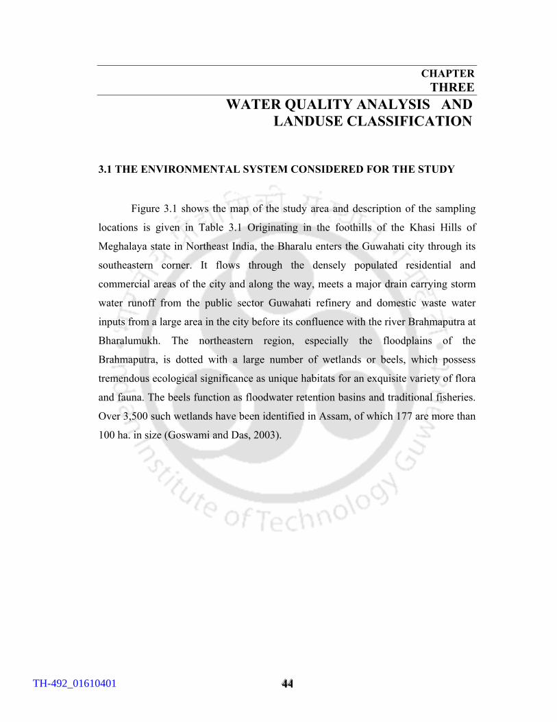
444444

CHAPTER THREE WATER QUALITY ANALYSIS AND LANDUSE CLASSIFICATION 3.1 THE ENVIRONMENTAL SYSTEM CONSIDERED FOR THE STUDY

Figure 3.1 shows the map of the study area and description of the sampling

locations is given in Table 3.1 Originating in the foothills of the Khasi Hills of

Meghalaya state in Northeast India, the Bharalu enters the Guwahati city through its

southeastern corner. It flows through the densely populated residential and

commercial areas of the city and along the way, meets a major drain carrying storm

water runoff from the public sector Guwahati refinery and domestic waste water

inputs from a large area in the city before its confluence with the river Brahmaputra at

Bharalumukh. The northeastern region, especially the floodplains of the

Brahmaputra, is dotted with a large number of wetlands or beels, which possess

tremendous ecological significance as unique habitats for an exquisite variety of flora

and fauna. The beels function as floodwater retention basins and traditional fisheries.

Over 3,500 such wetlands have been identified in Assam, of which 177 are more than

100 ha. in size (Goswami and Das, 2003).

TH-492_01610401

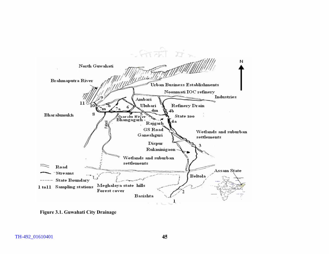
444555

Figure 3.1. Guwahati City Drainage

TH-492_01610401

444666

Table 3.1 Description of the sampling locations

Sample location No

Description

1 Basistha upstream area (hilly watershed).

2 Bifurcation point of Basistha and Bahini (opposite to a military office).

3 Rukmini Gaon (populated residential area).

4a Opposite to the Neelamani Phukan Park (commercial area).

4b Near RGB Road East Bye lane 8 (residential area).

4m Opposite to Jonali Path (adjoining urban traffic zone)

5 Bhangagarh bridge (busy street crossing )

6 Nepali Mandir-Rehabari (commercial area)

7a Chabipool –Natun Basti (residential commercial area)

7b Near Guwahati Koborosthan Masjid-Fatasil (busy Market area)

7m Meeting point of 7A &7B at Fatasil (drainage confluence)

8 Bharalu sluice gate (500m before discharge point to the main river)

9 Brahmaputra river (before the confluence of Bharalu).

10 Bharalu river (just before joining Brahmaputra).

11 Downstream of Brahmaputra (after confluence of Bharalu).

(Also refer to Figure 3.1 for graphical location of sampling points). 3.2 MATERIALS AND METHODS

Bharalu river was sampled for the period from December 2003 to April 2005

(December ’03, April ’04, August ’04, October’04, December’04, February ’05, April

’05) from, the above15 stations. For convenience of discussion, the sampling periods

have been classified as:

December: Winter

February : Dry

April : Pre monsoon

August : Receding monsoon

October : Post monsoon.

TH-492_01610401

444777

Sampling points were selected considering the following points:

• The origin of the watershed where no pollutants are expected

• The intermediate points which serve as the major drainage points of wastes as

inputs

• Confluence with the main river

Samples of 5 liters each were collected manually in pre-cleaned polyethylene bottles

3.2.1 ANALYTICAL METHODS AND INSTRUMENTS

pH, Conductivity and Total Dissolved Solids were measured soon after the

collection of the samples using digital meters. Total alkalinity was determined by

titrating the sample with 0.02 N H2SO4 using methyl orange as indicator and hardness

by EDTA titrimetric method. Concentration of chloride was obtained by

Argentometric method. DO was determined by the modified wrinkler method and

BOD by BOD method. Determination of other chemical components was carried out

by spectrophotometric method as follows: total phosphorus by digestion and

measurement with molybdophosphoric reagent; total iron measurement with o-

phenanthrolene reagent, aluminum using erichrome cyanine-R and sulphate by

turbidimetry with barium chloride reagent. Concentrations of sodium, potassium and

calcium were determined by flame photometer and total solids were determined by

gravimetric method. All the parameters were determined following recommended

analytical methods of APHA 1998. Hardness, Chloride, DO and BOD were analyzed

following the titration methods discussed in the Standard methods (APHA, 1998). 3.2.2 RECOMMENDEDWATER QUALITY CRITERIA

Standards of acceptable limits of surface water pollutants are presented in

Table 3.2. Desirable level is the requirement for the cleanest water, which can be used

for drinking purpose, and maximum permissible level is that needed for irrigation

purpose. Above the maximum permissible level is the objectionable level.

After analysis pollutant concentrations were tabulated and presented

graphically. Values were standardized between 0 and 1 in such a way that maximum

permissible limit corresponds to a value of 1 and desirable limit corresponds to a

value of 0. This representation was done to produce the levels of pollutants of each

location in one single plot. The level above 1 corresponds to the objectionable level.

TH-492_01610401

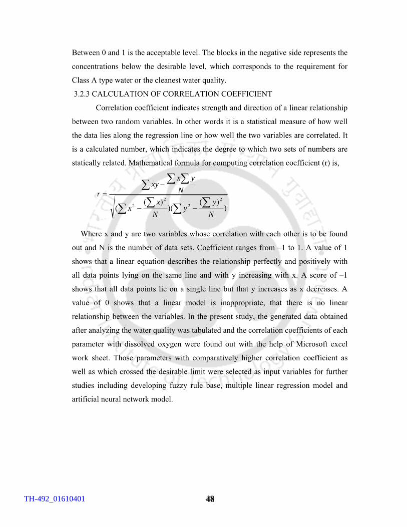
444888

Between 0 and 1 is the acceptable level. The blocks in the negative side represents the

concentrations below the desirable level, which corresponds to the requirement for

Class A type water or the cleanest water quality.

3.2.3 CALCULATION OF CORRELATION COEFFICIENT

Correlation coefficient indicates strength and direction of a linear relationship

between two random variables. In other words it is a statistical measure of how well

the data lies along the regression line or how well the two variables are correlated. It

is a calculated number, which indicates the degree to which two sets of numbers are

statically related. Mathematical formula for computing correlation coefficient (r) is,

∑ ∑ ∑∑∑ ∑ ∑

−−

−=

))(

)()(

(2

22

2

Ny

yN

xx

Nyx

xyr

Where x and y are two variables whose correlation with each other is to be found

out and N is the number of data sets. Coefficient ranges from –1 to 1. A value of 1

shows that a linear equation describes the relationship perfectly and positively with

all data points lying on the same line and with y increasing with x. A score of –1

shows that all data points lie on a single line but that y increases as x decreases. A

value of 0 shows that a linear model is inappropriate, that there is no linear

relationship between the variables. In the present study, the generated data obtained

after analyzing the water quality was tabulated and the correlation coefficients of each

parameter with dissolved oxygen were found out with the help of Microsoft excel

work sheet. Those parameters with comparatively higher correlation coefficient as

well as which crossed the desirable limit were selected as input variables for further

studies including developing fuzzy rule base, multiple linear regression model and

artificial neural network model.

TH-492_01610401

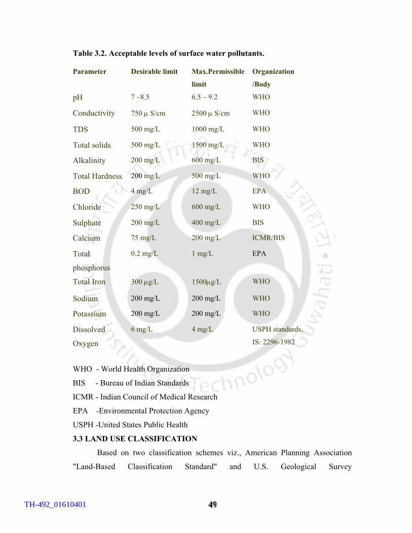
444999

Table 3.2. Acceptable levels of surface water pollutants.

WHO - World Health Organization

BIS - Bureau of Indian Standards

ICMR - Indian Council of Medical Research

EPA -Environmental Protection Agency

USPH -United States Public Health

3.3 LAND USE CLASSIFICATION

Based on two classification schemes viz., American Planning Association

"Land-Based Classification Standard" and U.S. Geological Survey

Parameter Desirable limit Max.Permissible

limit

Organization

/Body

pH 7 –8.5 6.5 – 9.2 WHO

Conductivity 750 µ S/cm 2500 µ S/cm WHO

TDS 500 mg/L 1000 mg/L WHO

Total solids 500 mg/L 1500 mg/L WHO

Alkalinity 200 mg/L 600 mg/L BIS

Total Hardness 200 mg/L 500 mg/L WHO

BOD 4 mg/L 12 mg/L EPA

Chloride 250 mg/L 600 mg/L WHO

Sulphate 200 mg/L 400 mg/L BIS

Calcium 75 mg/L 200 mg/L ICMR/BIS

Total

phosphorus

0.2 mg/L 1 mg/L EPA

Total Iron 300 µg/L 1500µg/L WHO

Sodium 200 mg/L 200 mg/L WHO

Potassium 200 mg/L 200 mg/L WHO

Dissolved

Oxygen

6 mg/L 4 mg/L USPH standards,

IS: 2296-1982

TH-492_01610401

555000

"Land-Use/Land-Cover Classification System for Use with Remotely Sensed Data",

the USGS scheme was adopted for the study with slight modifications in level II

classification of the various land uses. This scheme is resources based and not just

area based which provides scope for effective watershed model development.

Procedure adopted for urban land use classification

3.3.1 GEOMETRIC CORRECTION

The LISS – 3 image purchased from NRSA was geometrically registered to

Polyconic/Everest projection system with Toposheets No. N 78/12 and N 78/16 and

GPS navigational survey.

3.3 2 IMAGE ENHANCEMENT

Nonlinear contrast enhancement technique, also known as uniform distribution stretch

is adopted to make features like vegetation, land, water, and habitation. This type of

stretching applies the greatest contrast enhancement to the range of DNs occurring

most frequently in the reflectance histogram, resulting in a loss of information in the

white and black ranges, the loss being not so severe as in the case of a linear contrast

stretch. Non-linear stretch is applied to standard FCC of the image. Conventionally,

three primary colours, viz., blue, green, and red, are used in the green, red, and

infrared bands, respectively, to generate a standard FCC.

3.3.3 IMAGE CLASSIFICATION

A Multispectral classification is performed in FCC image of Guwahati area by

supervised classification method. The spectral reflectance data is extracted to define

the different land-use classes. More than 25 training sample were collected for each

class to get the proper spectral signature. The data derived from these training

samples are utilized as the basis for classification.

ERDAS spectral profile was extensively used to identify the correct spectral

signature for different classes. Supervised classification was performed with

MAXIMUM LIKELYHOOD algorithm. The spectral separability and contingency of

those training areas chosen are analyzed. Overall Accuracy was assessed using error

matrix. Classified map data of overall accuracy 95.8% in terms of geographic and

spectral similarity with ground truth is accepted as standard for the Guwahati city.

TH-492_01610401

555111

3.3.4 FIELD VERIFICATION

The standard classified map generated from IRS LISS-3 was further verified and

compared in the following ways: IRS LISS-III image of 23.5m resolutions was

merged with IRS PAN of 5.8m resolutions and land-use/land-cover feature was

compared. Classified data of year 2003 as found from LISS 3 imagery were compared

with 2000 and 1998 of LISS III imageries. Field survey was carried out with GPS

handset to collect critical location to verify those points.

3.3.5 GIS MODEL DEVELOPED

Geo Graphical information system developed for this study using ARC GIS

platform has four layers of information. The soil layer, land use pattern map (Figure

3.2) derived from remote sensing imageries, river and road network, contours using

topo sheets are embedded in different layers. Using GIS, the catchment is delineated

into sub catchments for each node of observations and the details are presented in

Table 3.3 (Wang and Hjelmfelt 1998). Different layers are used to study the influence

of catchment characteristics over the water quality data.

3.5 SUMMARY

Laboratory analysis was carried for the water samples collected from selected

locations of River Bharalu for assessing its pollution status. This was also aimed to

identify the sensitive parameters that adversely affect the system studied and also to

identify the sensitive locations. Correlation coefficients of the parameters were found

out to get an idea about the highly correlated parameters and also to decide the input

parameters to be selected for dissolved oxygen prediction modeling.

TH-492_01610401

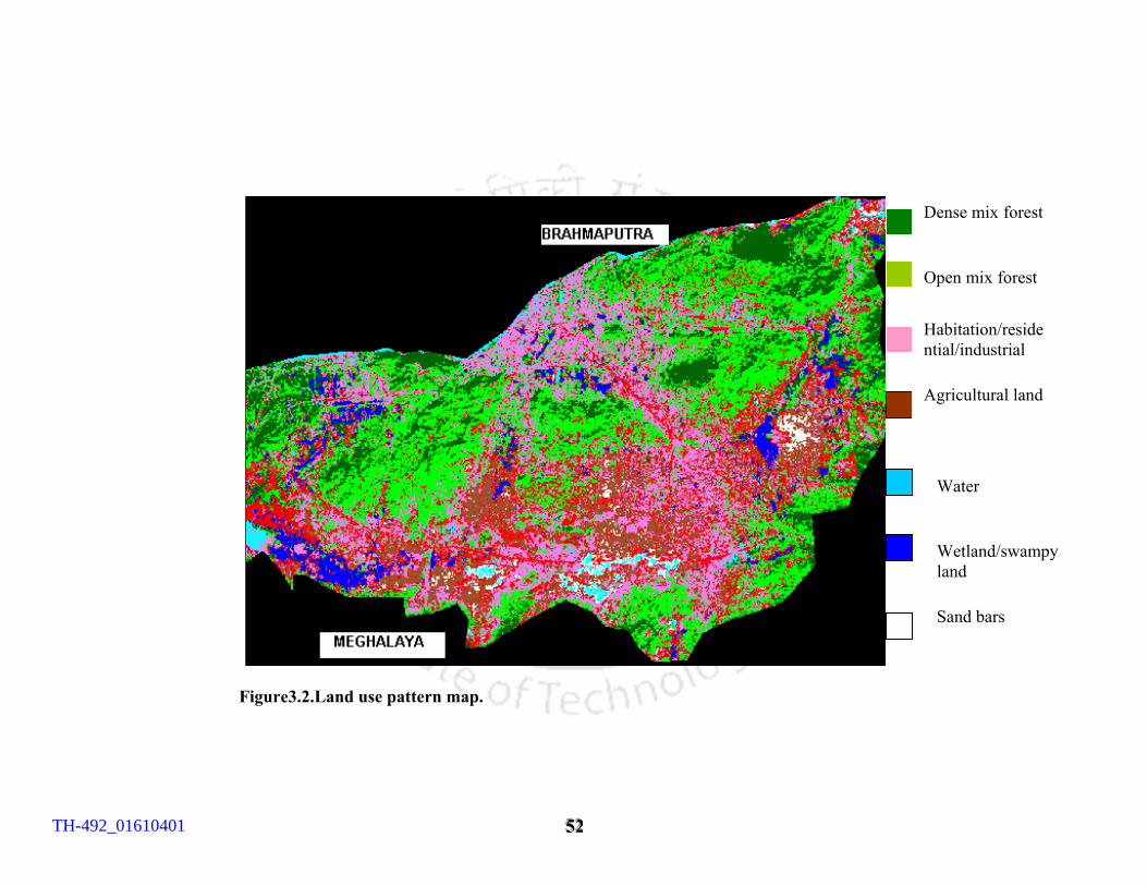
555222

Figure3.2.Land use pattern map.

Dense mix forest

Open mix forest

Habitation/residential/industrial

Agricultural land

Water

Wetland/swampy land

Sand bars

TH-492_01610401

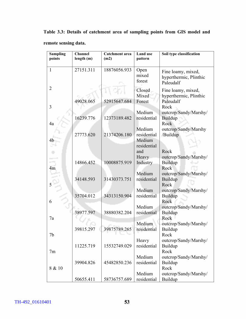
555333

Table 3.3: Details of catchment area of sampling points from GIS model and

remote sensing data.

Sampling points

Channel length (m)

Catchment area (m2)

Land use pattern

Soil type classification

1 27151.311 18876056.933 Open mixed forest

Fine loamy, mixed, hyperthermic, Plinthic Paleudalf

2

49028.065 52915647.684

Closed Mixed Forest

Fine loamy, mixed, hyperthermic, Plinthic Paleudalf

3

16239.776 12373189.482 Medium residential

Rock outcrop/Sandy/Marshy/ Buildup

4a


Rock outcrop/Sandy/Marshy /Buildup

4b

14866.452 10008875.919

Medium residential and Heavy Industry


4m



5



6



7a



7b

11225.719 15532749.029 Heavy residential


7m



8 & 10



TH-492_01610401

555444

CHAPTER FOUR RESULTS AND DISCUSSION ON WATER QUALITY ANALYSIS 4.1 WATER QUALITY ANALYSIS

Location1 is the origin of River Bharalu ahead of Basistha with a catchment

area of 20 km2 of hilly watershed with open mixed forest and fine loamy soil.

Location 1 meets the requirements for class A type quality (Figure 4.1) except for

total phosphorus, total iron, and chemical oxygen demand during the summer season

after 3 days of heavy rain. The pH of all the samples were within the permissible

levels with a range of (6.84 – 7.68), the minimum value being for the samples

collected during April’04 after the premonsoon shower with maximum value of 7.68

during December’04. Dissolution of CO2 from the atmosphere during the

premonsoon shower could be the reason for comparatively lower values of pH than

the dry season. Values of conductivity ranged from 44 µS/cm to 104 µS/cm which are

well within the desirable level of 750 µS/cm. High ionic concentrations (104 mg/L)

during premonsoon shower indicates dissolution of ion rich runoff water from the

catchment area, followed by dilution during monsoon season, and getting

concentrated during the low flow period. Increasing trend during the low flow

indicates the presence of subsurface flow, which is rich in ion via rock dissolution

also. Concentration of total dissolved solids varied from 22mg/L to 67 mg/L, which

showed similar trend as conductivity. TS (Total solids) varied from 52mg/l during the

driest season in February’05 to 450 mg/L during the monsoon season in August’05.

Elevated levels during the monsoon season show the effect of turbulence caused by

the flow. Alkalinities were in the range of 22 mg/L as CaCO3 in August’04 to 83

mg/L as CaCO3 during the premonsoon shower. Values of hardness varied from 8

mg/L during the winter season to 32 mg/L during the premonsoon shower.

Comparatively higher levels in conductivity, TDS (total dissolved solids), alkalinity

and hardness during the premonsoon shower indicate presence of dissolved salts

TH-492_01610401

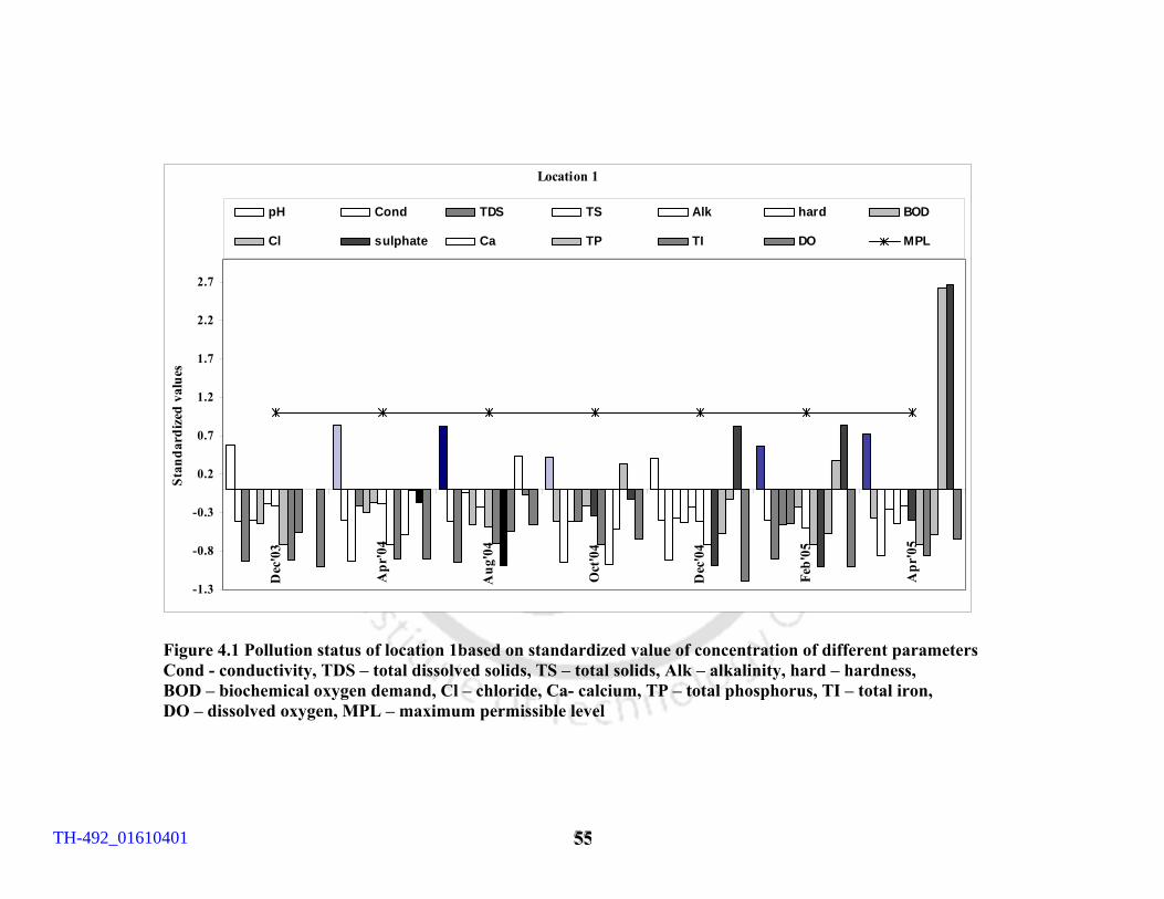
555555

Location 1

-1.3

-0.8

-0.3

0.2

0.7

1.2

1.7

2.2

2.7D

ec'0

3

Apr

'04

Aug

'04

Oct

'04

Dec

'04

Feb'

05

Apr

'05

Stan

dard

ized

val

ues

pH Cond TDS TS Alk hard BOD

Cl sulphate Ca TP TI DO MPL

Figure 4.1 Pollution status of location 1based on standardized value of concentration of different parameters Cond - conductivity, TDS – total dissolved solids, TS – total solids, Alk – alkalinity, hard – hardness, BOD – biochemical oxygen demand, Cl – chloride, Ca- calcium, TP – total phosphorus, TI – total iron, DO – dissolved oxygen, MPL – maximum permissible level

TH-492_01610401

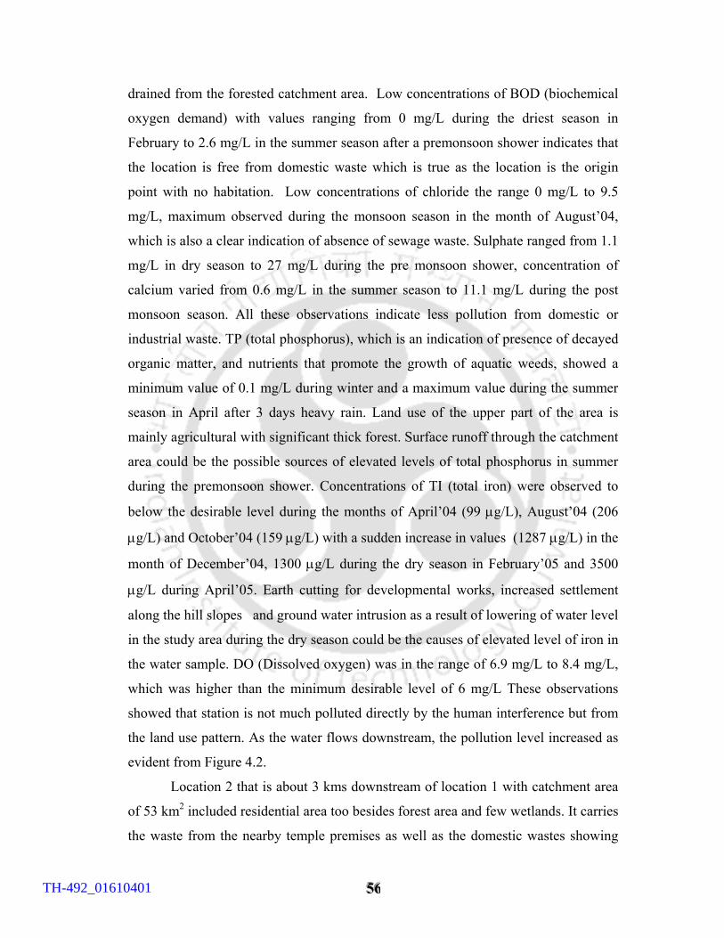
555666

drained from the forested catchment area. Low concentrations of BOD (biochemical

oxygen demand) with values ranging from 0 mg/L during the driest season in

February to 2.6 mg/L in the summer season after a premonsoon shower indicates that

the location is free from domestic waste which is true as the location is the origin

point with no habitation. Low concentrations of chloride the range 0 mg/L to 9.5

mg/L, maximum observed during the monsoon season in the month of August’04,

which is also a clear indication of absence of sewage waste. Sulphate ranged from 1.1

mg/L in dry season to 27 mg/L during the pre monsoon shower, concentration of

calcium varied from 0.6 mg/L in the summer season to 11.1 mg/L during the post

monsoon season. All these observations indicate less pollution from domestic or

industrial waste. TP (total phosphorus), which is an indication of presence of decayed

organic matter, and nutrients that promote the growth of aquatic weeds, showed a

minimum value of 0.1 mg/L during winter and a maximum value during the summer

season in April after 3 days heavy rain. Land use of the upper part of the area is

mainly agricultural with significant thick forest. Surface runoff through the catchment

area could be the possible sources of elevated levels of total phosphorus in summer

during the premonsoon shower. Concentrations of TI (total iron) were observed to

below the desirable level during the months of April’04 (99 µg/L), August’04 (206

µg/L) and October’04 (159 µg/L) with a sudden increase in values (1287 µg/L) in the

month of December’04, 1300 µg/L during the dry season in February’05 and 3500

µg/L during April’05. Earth cutting for developmental works, increased settlement

along the hill slopes and ground water intrusion as a result of lowering of water level

in the study area during the dry season could be the causes of elevated level of iron in

the water sample. DO (Dissolved oxygen) was in the range of 6.9 mg/L to 8.4 mg/L,

which was higher than the minimum desirable level of 6 mg/L These observations

showed that station is not much polluted directly by the human interference but from

the land use pattern. As the water flows downstream, the pollution level increased as

evident from Figure 4.2.

Location 2 that is about 3 kms downstream of location 1 with catchment area

of 53 km2 included residential area too besides forest area and few wetlands. It carries

the waste from the nearby temple premises as well as the domestic wastes showing

TH-492_01610401

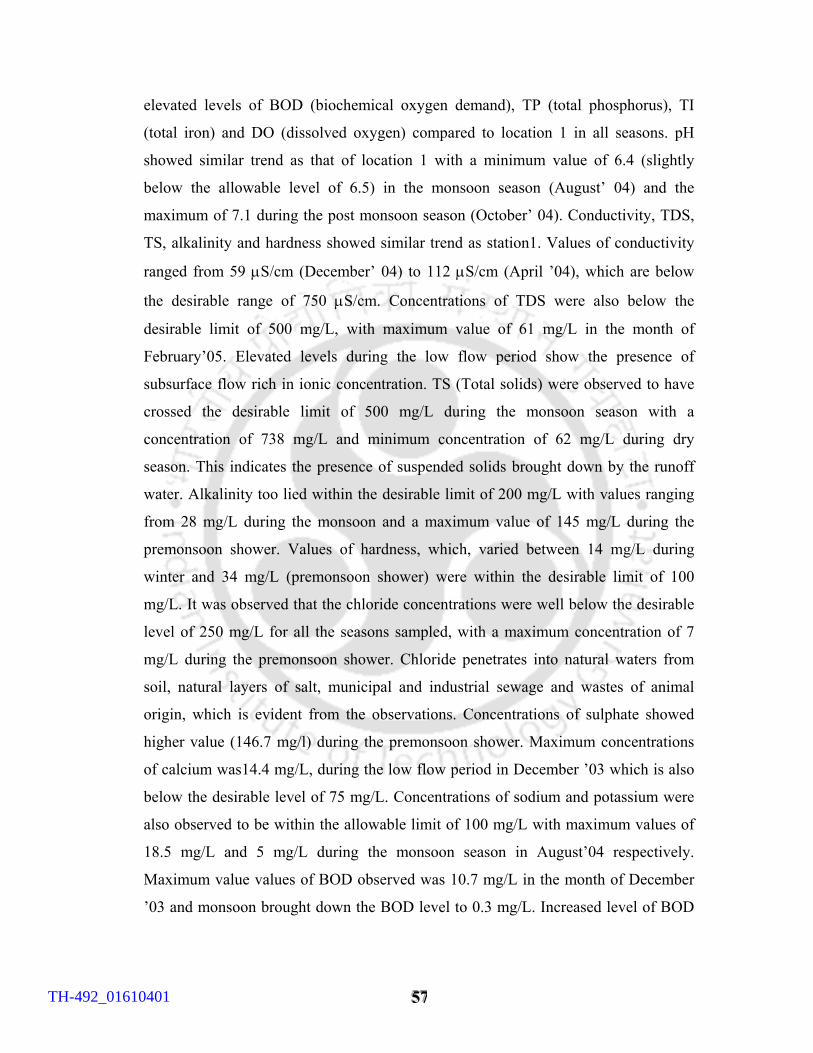
555777

elevated levels of BOD (biochemical oxygen demand), TP (total phosphorus), TI

(total iron) and DO (dissolved oxygen) compared to location 1 in all seasons. pH

showed similar trend as that of location 1 with a minimum value of 6.4 (slightly

below the allowable level of 6.5) in the monsoon season (August’ 04) and the

maximum of 7.1 during the post monsoon season (October’ 04). Conductivity, TDS,

TS, alkalinity and hardness showed similar trend as station1. Values of conductivity

ranged from 59 µS/cm (December’ 04) to 112 µS/cm (April ’04), which are below

the desirable range of 750 µS/cm. Concentrations of TDS were also below the

desirable limit of 500 mg/L, with maximum value of 61 mg/L in the month of

February’05. Elevated levels during the low flow period show the presence of

subsurface flow rich in ionic concentration. TS (Total solids) were observed to have

crossed the desirable limit of 500 mg/L during the monsoon season with a

concentration of 738 mg/L and minimum concentration of 62 mg/L during dry

season. This indicates the presence of suspended solids brought down by the runoff

water. Alkalinity too lied within the desirable limit of 200 mg/L with values ranging

from 28 mg/L during the monsoon and a maximum value of 145 mg/L during the

premonsoon shower. Values of hardness, which, varied between 14 mg/L during

winter and 34 mg/L (premonsoon shower) were within the desirable limit of 100

mg/L. It was observed that the chloride concentrations were well below the desirable

level of 250 mg/L for all the seasons sampled, with a maximum concentration of 7

mg/L during the premonsoon shower. Chloride penetrates into natural waters from

soil, natural layers of salt, municipal and industrial sewage and wastes of animal

origin, which is evident from the observations. Concentrations of sulphate showed

higher value (146.7 mg/l) during the premonsoon shower. Maximum concentrations

of calcium was14.4 mg/L, during the low flow period in December ’03 which is also

below the desirable level of 75 mg/L. Concentrations of sodium and potassium were

also observed to be within the allowable limit of 100 mg/L with maximum values of

18.5 mg/L and 5 mg/L during the monsoon season in August’04 respectively.

Maximum value values of BOD observed was 10.7 mg/L in the month of December

’03 and monsoon brought down the BOD level to 0.3 mg/L. Increased level of BOD

TH-492_01610401

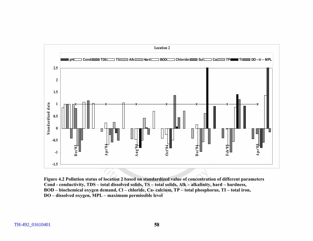
555888

Location 2

-1.5

-1

-0.5

0

0.5

1

1.5

2

2.5

Dec

'03

Apr

'04

Aug

'04

Oct

'04

Dec

'04

Feb'

05

Apr

'05

Stan

dard

ized

dat

a

pH Cond TDS TS Alk Hard BOD Chloride Sul Ca TP TI DO MPL

Figure 4.2 Pollution status of location 2 based on standardized value of concentration of different parameters Cond - conductivity, TDS – total dissolved solids, TS – total solids, Alk – alkalinity, hard – hardness,

BOD – biochemical oxygen demand, Cl – chloride, Ca- calcium, TP – total phosphorus, TI – total iron, DO – dissolved oxygen, MPL – maximum permissible level

TH-492_01610401

555999

indicates increased level of organic waste with time and lack of dilution during low

flow period. Concentrations of TP exceeded the maximum allowable limit during the

flood in October ’04 (1.3 mg/L) and during the summer season (1.3 mg/L) after 3

days heavy rain. An elevated level of total phosphorus in December ’03 reflects the

presence of aquatic weeds in the location. Water passing through the wetlands and the

agricultural area might have increased the total phosphorus level during the flood in

October’04 and the premonsoon shower in April ‘05. Total iron seemed to be higher

than the maximum permissible level during the month of December’04 (7260 µg/L)

February’05 (2000 µg/L), and April’05 (8900 µg/L). Frequent earth cutting and

ground water intrusion (base flow) during the dry season could be the possible causes

of increased levels of total iron. Dissolved oxygen did not meet the minimum

allowable requirement of 4 mg/L during the low periods in December’03 (3.7 mg/L)

and in February’05 (3.6 mg/L) At other times of sampling, DO varied from 5.1 mg/L

to 7.3 mg/L.

Trend of increasing pollution with time and distance can be evident from

Figure 4.3 for location 3. This location with catchment area of about 12 km2 is

surrounded by residential as well as industrial area and the river receives the

industrial waste as well as the domestic waste without any treatment resulting in

increased level of BOD and TP beyond the maximum permissible limit and low

values of DO below the minimum permissible limit of 4 mg/L.The pH values were

found to be in the acidic range during the monsoon season in August’04 with a value

of 3.45 and with the values of 6.65 and 6.62 during the premonsoon showers in

April’04 an April ’05 respectively. Alkalinity was observed to be very low in the

monsoon season in August ’04 (11 mg/L) with a maximum concentration during the

premonsoon shower in April ’04 (328 mg/L), which crossed the desirable level of 200 mg/L. Alkalinity is important for fish and aquatic life as it buffers against rapid pH

changes. Minimum required buffering capacity for the protection of aquatic life is 20

mg/L. Location 3 did not meet this requirement in the month of August and the low

alkalinity indicated corrosive water. Precipitation of CaCO3, decomposition of plant materials and the acidic nature of rainfall caused by atmospheric carbon dioxide and

TH-492_01610401

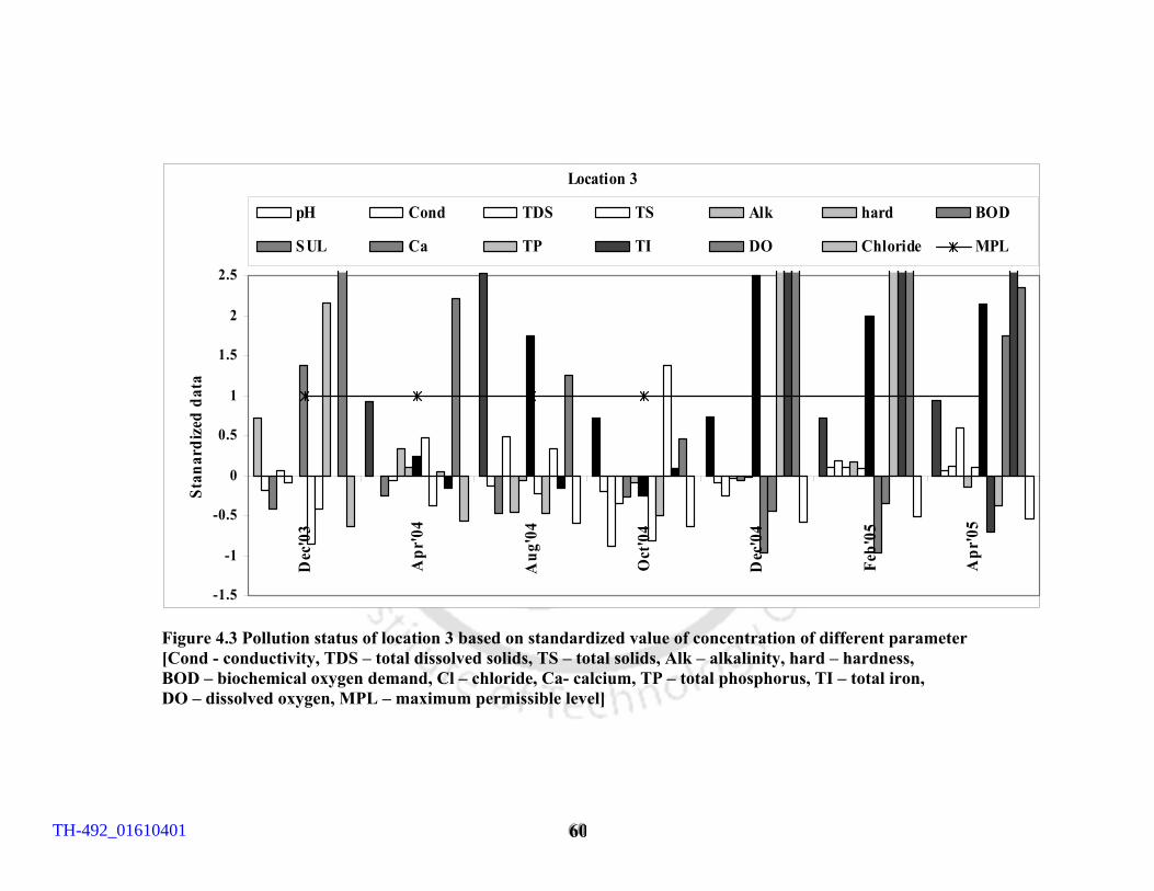
666000

Location 3

-1.5

-1

-0.5

0

0.5

1

1.5

2

2.5

Dec

'03

Apr

'04

Aug

'04

Oct

'04

Dec

'04

Feb'

05

Apr

'05

Stan

ardi

zed

data

pH Cond TDS TS Alk hard BOD

SUL Ca TP TI DO Chloride MPL

Figure 4.3 Pollution status of location 3 based on standardized value of concentration of different parameter

[Cond - conductivity, TDS – total dissolved solids, TS – total solids, Alk – alkalinity, hard – hardness, BOD – biochemical oxygen demand, Cl – chloride, Ca- calcium, TP – total phosphorus, TI – total iron, DO – dissolved oxygen, MPL – maximum permissible level]

TH-492_01610401

666111

other airborne pollutants especially oxide gases of sulphur and nitrogen could be the

causes of low alkalinity (Hairstone, 1995). In this case the low alkalinity

accompanied by the drop in pH value confirms that the precipitation of CaCO3 could

be the cause. Maximum conductivity was observed during the dry season in

February’ 05 with a value of 909 µS/cm. Total dissolved solids showed the similar

trend as conductivity with values ranging from 54 mg/l during October’ 04 to dry

592mg/L during the season in February’ 05 which indicates the presence of ion rich

subsurface flow during low flow period. Total solids were least (136 mg/L) during the

post monsoon season in February’05 and maximum (1093 mg/L) during the

premonsoon shower in April’ 05 which is the clear indication of presence suspended

solids brought down by runoff. Values of hardness were found to be above the

desirable limit of 100 mg/L during the summer seasons in April ‘04 and April ’05

(140 mg/L each) and in February ’05 (130 mg/L). Hardness was observed to be the

least during the flood in October ’04 with a concentration of 64 mg/L, which could be

due to the natural attenuation. BOD was observed to be least in October ’04 (2 mg/L)

and for all other seasons it was observed to be high with concentrations ranging from

12 mg/l to 24 mg/l with highest concentration during the low flow period in

December’ 04.This indicates the presence of organic mater due to the domestic as

well as industrial wastes. Concentration of chloride was below the desirable limit of

250 mg/L for all seasons with maximum value of 69 mg/L during the low flow period

in February’05. This indicates lack of dilution during the low flow period. Sulphate

was observed to surpass the desirable level of 200 mg/L during the premonsoon

shower in April ’04 with a value of 292 mg/L. Concentration was the least (6.52

mg/l) during the low flow period in December ’04. Elevated levels of sulphates

during the rain after the dry spell could be due to fertilizers and refuse leachates.

Concentration of calcium was with in the desirable level of 75 mg/L for all the

seasons with highest concentration 30 mg/L in the month of February ’05 (low flow

period). It was observed that concentrations of total phosphorus was above the

desirable level of 0.2 mg/L for all seasons with maximum concentration of 3.8 mg/L

in February ’05 and minimum concentration of 0.23 mg/L in April ’04. Runoffs

besides the aquatic weeds are the source of higher concentration of total phosphorus

TH-492_01610401

666222

during the flood. It was observed that after the flood, the concentrations of total iron

increased above the maximum permissible limit with values of 390 µg/L in August

‘04, 15000 µg/L in October ’04, 3400 µg/L in February ’05 and 9000 µg/L in April

’05. These elevated levels are likely to be due to ground water seepage. Water table

rises after the flood and in winter the predominant natural source of water in the study

area is the base flow. A rise in the concentration from 3400 µg/L in the month of

February ‘05 to 9000 µg/L in April ’05 was observed which could be due to the

frequent earth cutting in the nearby area followed by pre monsoon shower.

Concentration of sodium was observed to be within the safe limit of 50 mg/L in all

seasons except during the dry season in February ’05 when the concentration was

59.6 mg/L. Potassium was observed to be below the desirable limit with values

ranging from 8.5 mg/L during the monsoon season in August ’04 to 29 mg/L during

the dry season in February ’05. Dissolved oxygen didn’t meet the requirement for

minimum allowable level of 4 mg/L except in October ’04 (5.1 mg/L) with values

ranging from 0.1 mg/L in the month of December ‘04 to 3.5 mg/L in August

’04.Although the reaeration could replenish the DO during the rainy season to some

extent it could not bring it to a level more than 5.1 mg/L.

Similar to location 3, location 4(a) that receives the drainage from industries

as well as residential developments showed concentrations above the maximum

permissible limit for BOD, TP and TI while DO was below the minimum permissible

limit (Figure 4.4) TP and DO showed concentration beyond the permissible level

during the post monsoon season. pH value was in the acidic range during the

monsoon (August ’04) with a value of 5.9. For all other seasons, the pH values were

within the desirable level with values ranging from 6.7 to 7.1. Conductivity values

were with in the desirable level with a maximum value of 727 µS/cm in February ’05.

Total dissolved solids also lied within the desirable range of 500 mg/L with values

ranging from 172 mg/L (October’ 04) to 473 mg/L (February ’05). Total solids were

found to be the least (200 mg/L) during the post monsoon season in October ‘04 and

highest (612 mg/L) during the pre monsoon shower in April’05. Maximum value of

alkalinity (318 mg/L) was observed during the premonsoon shower in April ‘04,

TH-492_01610401

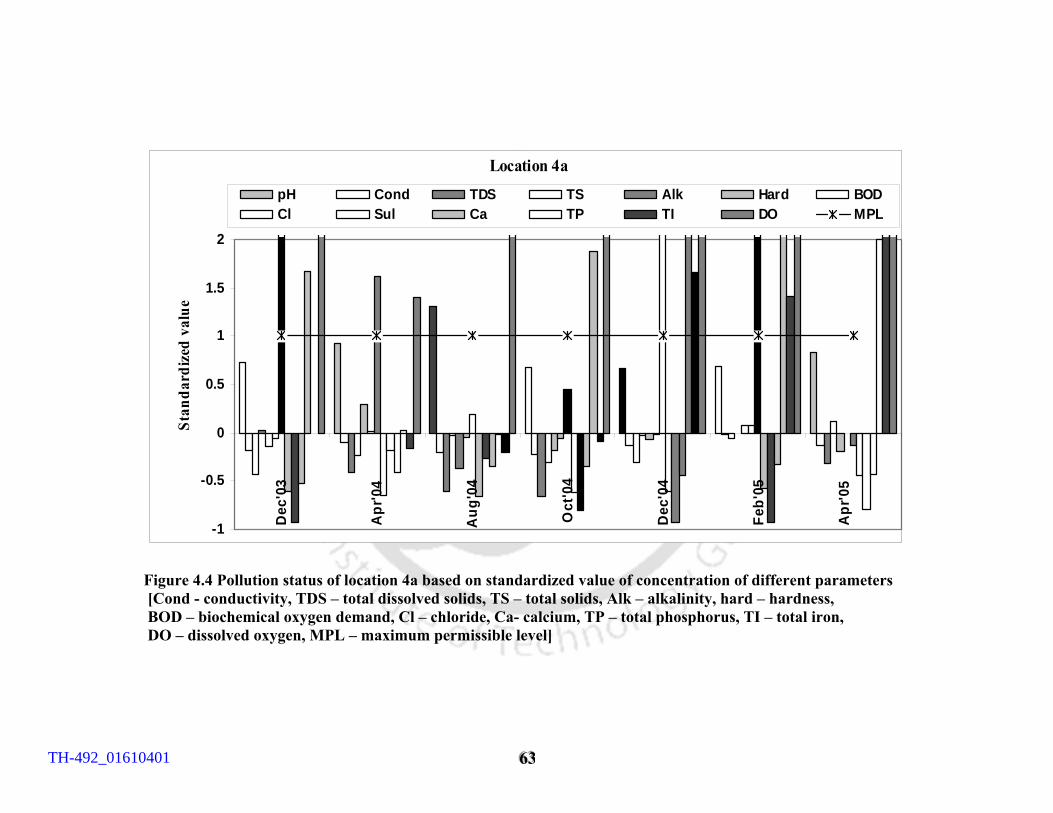
666333

Location 4a

-1

-0.5

0

0.5

1

1.5

2

Dec

'03

Apr

'04

Aug

'04

Oct

'04

Dec

'04

Feb'

05

Apr

'05

Stan

dard

ized

val

uepH Cond TDS TS Alk Hard BODCl Sul Ca TP TI DO MPL

Figure 4.4 Pollution status of location 4a based on standardized value of concentration of different parameters [Cond - conductivity, TDS – total dissolved solids, TS – total solids, Alk – alkalinity, hard – hardness,

BOD – biochemical oxygen demand, Cl – chloride, Ca- calcium, TP – total phosphorus, TI – total iron, DO – dissolved oxygen, MPL – maximum permissible level]

TH-492_01610401

666444

which crossed, the desirable level of 200 mg/L. Hardness was found to maximum

value in February ’05 (130 mg/L). BOD was maximum values (23.2 mg/L) in

December’ 04.concentrations beyond the permissible level, except during the

premonsoon shower in April’05 with a concentration of 3 mg/L.Natural attenuation is

observed to be the cause of reduction in BOD. Chloride concentrations were below

the desirable level of 250 mg/L with values ranging from 21 mg/L during the

monsoon in August ’04 to 94 mg/L in April ’05 which indicates that the sudden

downpour during the summer season might have washed down the refuse leachates as

the catchment area of the location is mainly residential. Sulphate also showed the

same trend as chloride for this location maximum concentrations of 165 mg/L during

the premonsoon shower in April’ 04. Calcium was also found to be below the

desirable level with maximum concentration of 34 mg/L in February ’05 with out

much seasonal variation in concentration. Concentrations of total phosphorus were

above the desirable level and even above the maximum allowable level for all seasons

except April ’04 (0.2 mg/L) and August ’04 (0.18 mg/L) with maximum value of 3.3

mg/L in February ‘05, which indicates the presence of aquatic weeds. Lower levels in

the monsoon season is the clear indication that there is no contribution from

catchment area and it is clear from the land use pattern that it is a residential area.

The concentrations of total iron was observed to be 2294 µg/L in December ‘04, 2000

µg/L in February ’05 and 3800 µg/L in April ’05. Subsurface flow could be the

source of increased level of total iron during the winter season in December and the

dry season in February ... Frequent hill cutting for the developmental activities also

might have contributed to the elevated levels of total iron in the month of April in the

summer season compared to the levels in December and February. Sodium was below

the desirable limit for all seasons with maximum concentration of 44.5 mg/L in

February ’05. Potassium was within the desirable limit with maximum 16.2 mg/L in

February ’05. DO concentration didn’t meet the minimum allowable level for any of

the seasons with values ranging from 0 mg/L in August ’04 3.2 mg/L in April ’04. As

in the case of location 3 the runoff combined with the aquatic weeds might have

increased the phosphorus concentration, which in turn increased the stress on the

TH-492_01610401

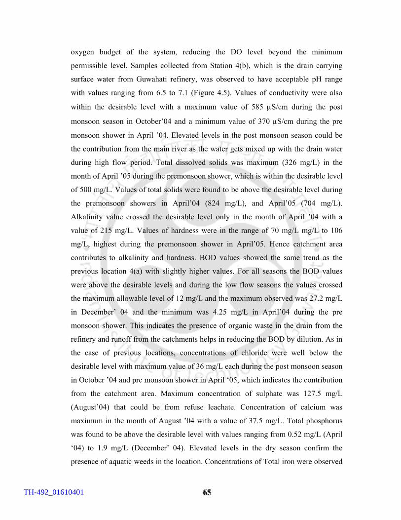
666555

oxygen budget of the system, reducing the DO level beyond the minimum

permissible level. Samples collected from Station 4(b), which is the drain carrying

surface water from Guwahati refinery, was observed to have acceptable pH range

with values ranging from 6.5 to 7.1 (Figure 4.5). Values of conductivity were also

within the desirable level with a maximum value of 585 µS/cm during the post

monsoon season in October’04 and a minimum value of 370 µS/cm during the pre

monsoon shower in April ’04. Elevated levels in the post monsoon season could be

the contribution from the main river as the water gets mixed up with the drain water

during high flow period. Total dissolved solids was maximum (326 mg/L) in the

month of April ’05 during the premonsoon shower, which is within the desirable level

of 500 mg/L. Values of total solids were found to be above the desirable level during

the premonsoon showers in April’04 (824 mg/L), and April’05 (704 mg/L).

Alkalinity value crossed the desirable level only in the month of April ’04 with a

value of 215 mg/L. Values of hardness were in the range of 70 mg/L mg/L to 106

mg/L, highest during the premonsoon shower in April’05. Hence catchment area

contributes to alkalinity and hardness. BOD values showed the same trend as the

previous location 4(a) with slightly higher values. For all seasons the BOD values

were above the desirable levels and during the low flow seasons the values crossed

the maximum allowable level of 12 mg/L and the maximum observed was 27.2 mg/L

in December’ 04 and the minimum was 4.25 mg/L in April’04 during the pre

monsoon shower. This indicates the presence of organic waste in the drain from the

refinery and runoff from the catchments helps in reducing the BOD by dilution. As in

the case of previous locations, concentrations of chloride were well below the

desirable level with maximum value of 36 mg/L each during the post monsoon season

in October ’04 and pre monsoon shower in April ‘05, which indicates the contribution

from the catchment area. Maximum concentration of sulphate was 127.5 mg/L

(August’04) that could be from refuse leachate. Concentration of calcium was

maximum in the month of August ’04 with a value of 37.5 mg/L. Total phosphorus

was found to be above the desirable level with values ranging from 0.52 mg/L (April

‘04) to 1.9 mg/L (December’ 04). Elevated levels in the dry season confirm the

presence of aquatic weeds in the location. Concentrations of Total iron were observed

TH-492_01610401

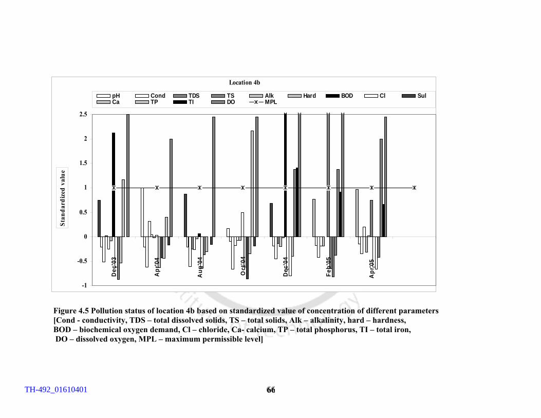
666666

Location 4b

-1

-0.5

0

0.5

1

1.5

2

2.5D

ec'0

3

Apr

'04

Aug

'04

Oct

'04

Dec

'04

Feb'

05

Apr

'05

Stan

dard

ized

val

ue

pH Cond TDS TS Alk Hard BOD Cl SulCa TP TI DO MPL

Figure 4.5 Pollution status of location 4b based on standardized value of concentration of different parameters [Cond - conductivity, TDS – total dissolved solids, TS – total solids, Alk – alkalinity, hard – hardness, BOD – biochemical oxygen demand, Cl – chloride, Ca- calcium, TP – total phosphorus, TI – total iron, DO – dissolved oxygen, MPL – maximum permissible level]

TH-492_01610401

666777

to have crossed the desirable level in December’ 04 (1996 µg/L), February ’05 (1400

µg/L) and April ’05 (1100 µg/L). Elevated concentrations of iron indicate ground

water seepage during the low flow season. But the concentrations are lower than that

of the previous locations, which could be due to the dilution with iron free wastewater

from the refinery. Very small concentrations of sodium and potassium were observed

with a maximum value of 20.6 mg/L in August ’04 and 11.9 mg/L in April ’05

respectively. Very low concentration dissolved oxygen (0.1 mg/L to 1.1 mg/l) was

observed. Presence of organic waste as well as the aquatic weeds increased the levels

of BOD and the total phosphorus, which in turn reduced the concentration of DO.

Increase in waste load can be evident from the observations (Figure 4.6) for

location 4m. Dissolved oxygen seemed to be below 4 mg/L throughout the year.

Except during the monsoon and the post monsoon, concentrations of parameters like

BOD, COD and TP were observed to be very high and found to be well above the

maximum permissible limits.pH values were within the range 6.15 (August ’04) to

7.25 (October ’04). During the monsoon season pH seemed to be in the acidic range

which could be due to the presence of humic substances. That indicates the

dissolution of CO2 of the atmosphere with the rainwater, which makes it acidic.

Values of conductivity and total dissolved solids were observed to be below the

permissible range with maximum values of 520 µS/cm and 338 mg/L in the month of

April ‘05.here also contribution from the catchment area is evident. Total solids was

observed to be above the desirable level in the months of December ‘03, August ’04

and April, 05 with concentrations of 700 mg/L, 1206 mg/L and 744 mg/L

respectively. For other seasons values were within the desirable level. Alkalinity was

found to be below the desirable level for all seasons except in April ’04 with a value

of 233 mg/L, which is possibly from the catchment, minimum value of 65 mg/L being

during the monsoon season in August ‘04, which could be due to dilution. Hardness

was observed to be maximum (102 mg/L) during the low flow in February ‘04, which

can be from subsurface flow as well as from the waste. BOD values were with in the

range of 3.5 mg/L in the month of August ’04 to 26.4 mg/L in the month of

December ’04 which is a clear indication of organic matter in the water samples.

TH-492_01610401

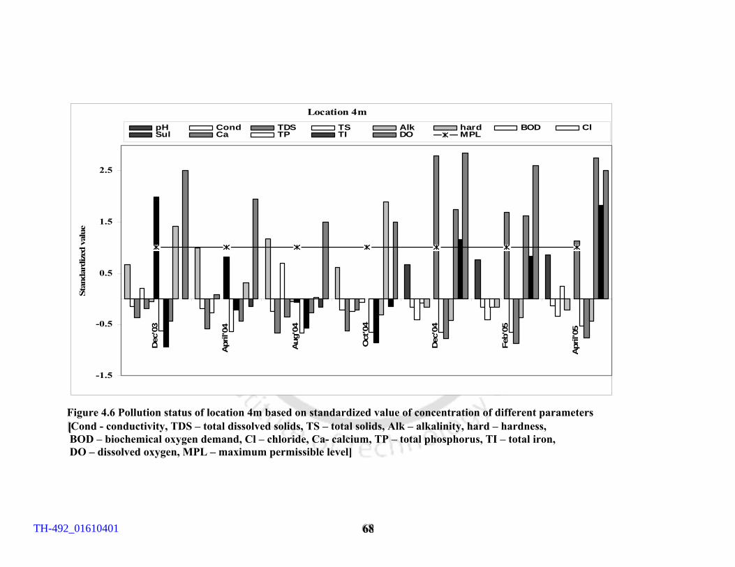
666888

Location 4m

-1.5

-0.5

0.5

1.5

2.5

Dec

'03

Apr

il'04

Aug

'04

Oct

'04

Dec

'04

Feb'

05

Apr

il'05

Stan

dard

ized

val

ue

pH Cond TDS TS Alk hard BOD ClSul Ca TP TI DO MPL

Figure 4.6 Pollution status of location 4m based on standardized value of concentration of different parameters [[[Cond - conductivity, TDS – total dissolved solids, TS – total solids, Alk – alkalinity, hard – hardness, BOD – biochemical oxygen demand, Cl – chloride, Ca- calcium, TP – total phosphorus, TI – total iron, DO – dissolved oxygen, MPL – maximum permissible level]

TH-492_01610401

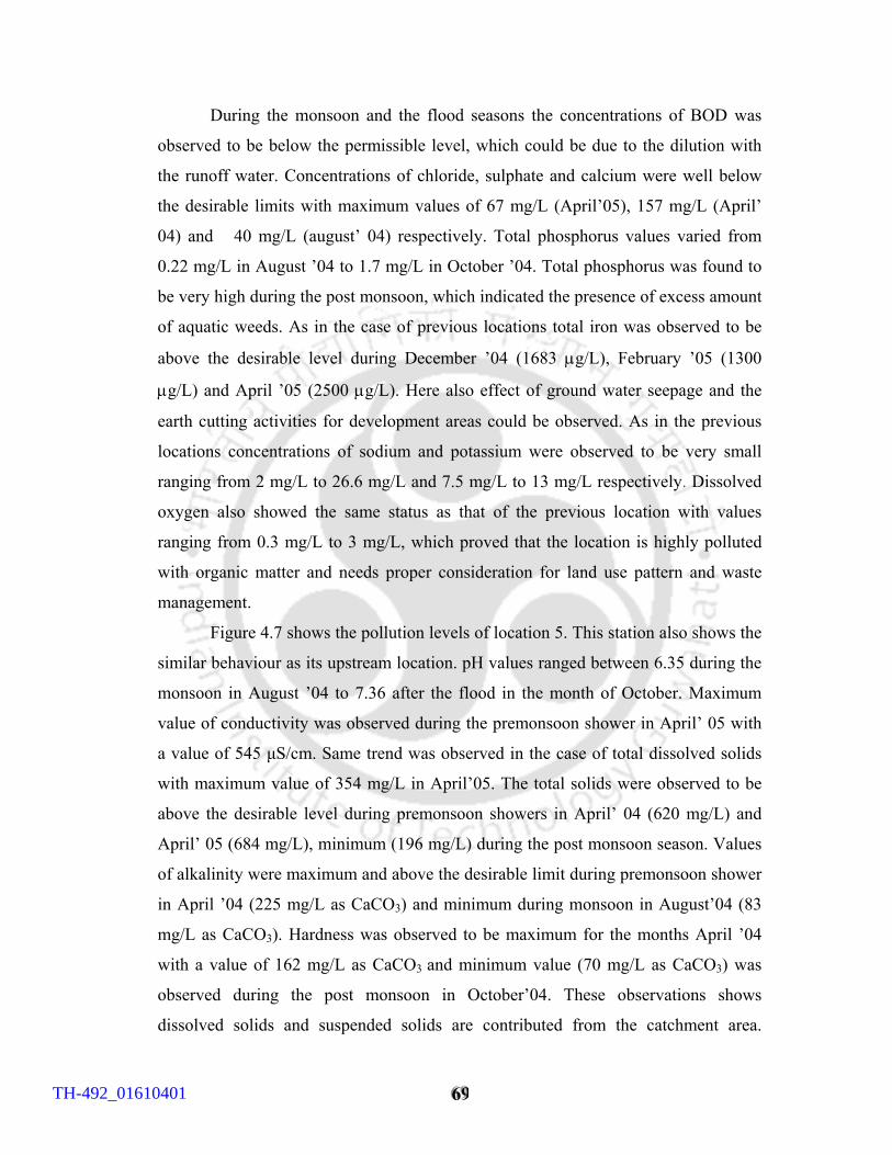
666999

During the monsoon and the flood seasons the concentrations of BOD was

observed to be below the permissible level, which could be due to the dilution with

the runoff water. Concentrations of chloride, sulphate and calcium were well below

the desirable limits with maximum values of 67 mg/L (April’05), 157 mg/L (April’

04) and 40 mg/L (august’ 04) respectively. Total phosphorus values varied from

0.22 mg/L in August ’04 to 1.7 mg/L in October ’04. Total phosphorus was found to

be very high during the post monsoon, which indicated the presence of excess amount

of aquatic weeds. As in the case of previous locations total iron was observed to be

above the desirable level during December ’04 (1683 µg/L), February ’05 (1300

µg/L) and April ’05 (2500 µg/L). Here also effect of ground water seepage and the

earth cutting activities for development areas could be observed. As in the previous

locations concentrations of sodium and potassium were observed to be very small

ranging from 2 mg/L to 26.6 mg/L and 7.5 mg/L to 13 mg/L respectively. Dissolved

oxygen also showed the same status as that of the previous location with values

ranging from 0.3 mg/L to 3 mg/L, which proved that the location is highly polluted

with organic matter and needs proper consideration for land use pattern and waste

management.

Figure 4.7 shows the pollution levels of location 5. This station also shows the

similar behaviour as its upstream location. pH values ranged between 6.35 during the

monsoon in August ’04 to 7.36 after the flood in the month of October. Maximum

value of conductivity was observed during the premonsoon shower in April’ 05 with

a value of 545 µS/cm. Same trend was observed in the case of total dissolved solids

with maximum value of 354 mg/L in April’05. The total solids were observed to be

above the desirable level during premonsoon showers in April’ 04 (620 mg/L) and

April’ 05 (684 mg/L), minimum (196 mg/L) during the post monsoon season. Values

of alkalinity were maximum and above the desirable limit during premonsoon shower

in April ’04 (225 mg/L as CaCO3) and minimum during monsoon in August’04 (83

mg/L as CaCO3). Hardness was observed to be maximum for the months April ’04

with a value of 162 mg/L as CaCO3 and minimum value (70 mg/L as CaCO3) was

observed during the post monsoon in October’04. These observations shows

dissolved solids and suspended solids are contributed from the catchment area.

TH-492_01610401

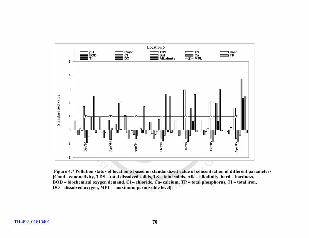
777000

Location 5

-2

-1

0

1

2

3

4

5

Dec

'03

Apr

'04

Aug

'04

Oct

'04

Dec

'04

Feb'

05

Apr

'05

Stan

dard

ized

val

uepH Cond TDS TS HardBOD Cl Sul Ca TPTI DO Alkalinity MPL

Figure 4.7 Pollution status of location 5 based on standardized value of concentration of different parameters [Cond - conductivity, TDS – total dissolved solids, TS – total solids, Alk – alkalinity, hard – hardness, BOD – biochemical oxygen demand, Cl – chloride, Ca- calcium, TP – total phosphorus, TI – total iron, DO – dissolved oxygen, MPL – maximum permissible level]

TH-492_01610401

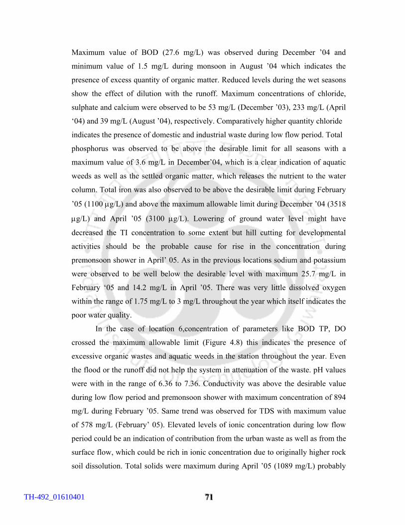
777111

Maximum value of BOD (27.6 mg/L) was observed during December ’04 and

minimum value of 1.5 mg/L during monsoon in August ’04 which indicates the

presence of excess quantity of organic matter. Reduced levels during the wet seasons

show the effect of dilution with the runoff. Maximum concentrations of chloride,

sulphate and calcium were observed to be 53 mg/L (December ’03), 233 mg/L (April

‘04) and 39 mg/L (August ’04), respectively. Comparatively higher quantity chloride

indicates the presence of domestic and industrial waste during low flow period. Total

phosphorus was observed to be above the desirable limit for all seasons with a

maximum value of 3.6 mg/L in December’04, which is a clear indication of aquatic

weeds as well as the settled organic matter, which releases the nutrient to the water

column. Total iron was also observed to be above the desirable limit during February

’05 (1100 µg/L) and above the maximum allowable limit during December ’04 (3518

µg/L) and April ’05 (3100 µg/L). Lowering of ground water level might have

decreased the TI concentration to some extent but hill cutting for developmental

activities should be the probable cause for rise in the concentration during

premonsoon shower in April’ 05. As in the previous locations sodium and potassium

were observed to be well below the desirable level with maximum 25.7 mg/L in

February ‘05 and 14.2 mg/L in April ’05. There was very little dissolved oxygen

within the range of 1.75 mg/L to 3 mg/L throughout the year which itself indicates the

poor water quality.

In the case of location 6,concentration of parameters like BOD TP, DO

crossed the maximum allowable limit (Figure 4.8) this indicates the presence of

excessive organic wastes and aquatic weeds in the station throughout the year. Even

the flood or the runoff did not help the system in attenuation of the waste. pH values

were with in the range of 6.36 to 7.36. Conductivity was above the desirable value

during low flow period and premonsoon shower with maximum concentration of 894

mg/L during February ’05. Same trend was observed for TDS with maximum value

of 578 mg/L (February’ 05). Elevated levels of ionic concentration during low flow

period could be an indication of contribution from the urban waste as well as from the

surface flow, which could be rich in ionic concentration due to originally higher rock

soil dissolution. Total solids were maximum during April ’05 (1089 mg/L) probably

TH-492_01610401

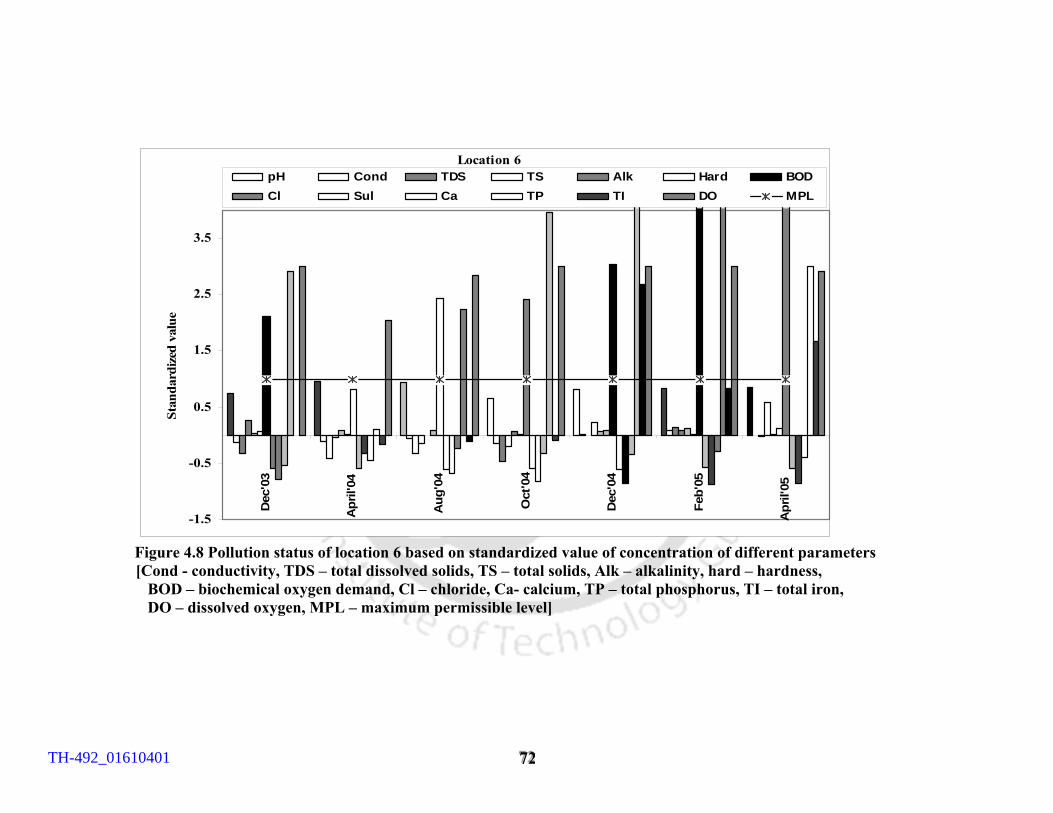
777222

Location 6

-1.5

-0.5

0.5

1.5

2.5

3.5

Dec

'03

Apr

il'04

Aug

'04

Oct

'04

Dec

'04

Feb'

05

Apr

il'05

Stan

dard

ized

val

uepH Cond TDS TS Alk Hard BODCl Sul Ca TP TI DO MPL


TH-492_01610401

777333

contributed from the catchment area. Alkalinity values were above the desirable level

except during August ’04 (199 mg/L) with maximum concentration of 248 mg/L in

February’ 05. Additional drainages from local industries and residential development

without any treatment contribute to elevated levels in alkalinity during low flow

period. Hardness values were above the desirable level for all seasons with maximum

value of 152 mg/L (April ’05), which indicates the contribution from land. BOD was

high throughout the seasons with values ranging from 10.5 mg/L (April’04) to 70

mg/L (February ’05). It was observed from land use pattern that location 6 is close to

industrial and railway establishments surrounded by large swamps. Higher values of

BOD in this location could be from the settled animal and human wastes carried by

the urban runoff during rain from streets and side walks, nutrients from leaves and

papers from residential areas, as well as the decayed organic matter. Maximum

concentrations of chloride, sulphate and calcium were, 51 mg/L (February ’05), 136

mg/L (April ’04) and 46 mg/L (October ’04) respectively. There was not much

seasonal variation for the concentration of chloride for this location. Increased

pollution is apparent from the increased level of concentration compared to the

previous stations. Higher concentration of sulphate during the premonsoon shower

indicates the contribution from land. Total phosphorus was found to be above the

maximum permissible level for all the seasons except during April ’04 (0.3 mg/L).

The values ranged from 1.98 mg/L (August ‘04) to 4.4 mg/L (February ’05). Sources

of elevated concentration could be the fertilizer runoff, human and animal waste,

domestic wastes with the use of detergents and industrial wastes. Elevated level of TP

during low flow indicates the presence of settled organic waste also due to the excess

growth of aquatic weeds. Like the previous stations concentration of TI seemed to be

very high during the low flow period in December’04 with a concentration of 3518

µg/L.During the low flow period in February’ 05 decrease in the concentration is

noticed (1300 µg/L) followed by a raise in the concentration during the pre monsoon

shower in April’05 (2300 µg/L). Here also the ground water seepage as well as the

developmental activities could be the probable cause for the increased level of Total

iron. Sodium and potassium were found to be below the desirable value with values

with maximum values of 43.3 mg/L during the dry season and 17.4 mg/L during

TH-492_01610401

777444

April ’05 respectively. Dissolved oxygen was found to be nil during low flow period

and very small quantities of dissolved oxygen were observed with values 1.9 mg/L

during April ’04, 0.3 mg/L in August ’04 and 0.2 mg/L in April ’05 as a result of

combined effect of aquatic weeds and organic matter.

Location 7(a) also showed the similar trend as station 6 for the parameters

BOD DO, total Phosphorus, and total Iron (Figure 4.9). All other parameters were

within the acceptable limit. Land use of this location covers partly agricultural lands,

residential complexes and huge medical campus facilities. The pH was within the

maximum allowable range with values varying from 6.73 (August ‘04) to 7.33 (April

’04). Maximum values of conductivity and TDS were 838 µS/cm (February ’05) and

546 mg/L (February ’04) respectively. Elevated levels during the low flow period

settled increased quantity of settled wastes. Maximum alkalinity was found to be 593

mg/L (April ’04). Hardness values were above the desirable level with maximum

value of 162 mg/L (April ’04). These observation shows that alkalinity and hardness

were contribute by the catchment area. Low flow period in February’05 was observed

to have highest BOD (51 mg/L), which is a clear indication of settle organic matter.

elevated levels during December ’04, February ’05 and April ’05 with values of

1287.4 µg/L, 1300 µg/L and 3500 µg/L respectively. Sodium and potassium were

within the allowable limit with maximum concentrations of 41.8 mg/L (February ’05)

and 14.5 mg/L (April ’05). Dissolved oxygen was nil during December ’03,

October’04, February ’05 and April ’05 with very low in concentration during April

’04 (1.7 mg/L), August ’04 (1.1 mg/L) and December ’04 (0.1 mg/L).

TH-492_01610401

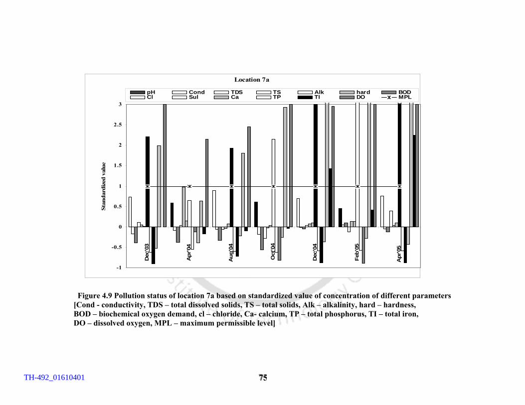
777555

Location 7a

-1

-0.5

0

0.5

1

1.5

2

2.5

3

Dec

'03

Apr

'04

Aug

'04

Oct

'04

Dec

'04

Feb'

05

Apr

'05

Stan

dard

ized

val

ue

pH Cond TDS TS Alk hard BODCl Sul Ca TP TI DO MPL

Figure 4.9 Pollution status of location 7a based on standardized value of concentration of different parameters [Cond - conductivity, TDS – total dissolved solids, TS – total solids, Alk – alkalinity, hard – hardness,

BOD – biochemical oxygen demand, cl – chloride, Ca- calcium, TP – total phosphorus, TI – total iron, DO – dissolved oxygen, MPL – maximum permissible level]

TH-492_01610401

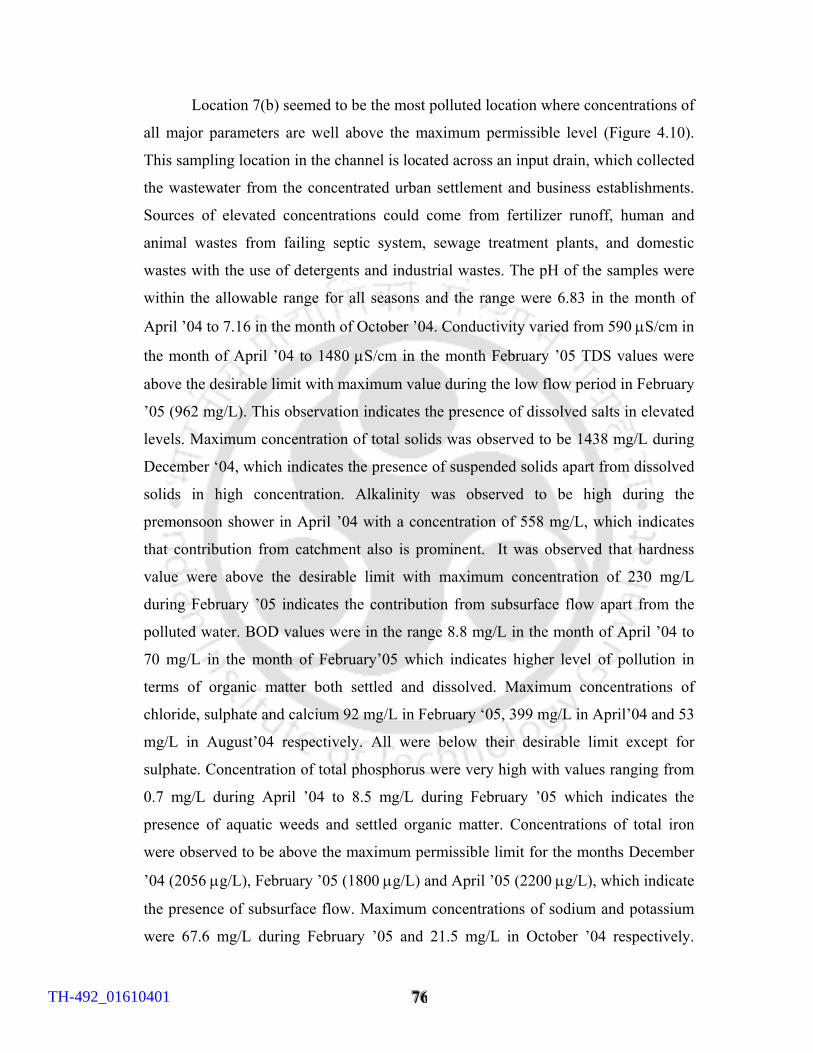
777666

Location 7(b) seemed to be the most polluted location where concentrations of

all major parameters are well above the maximum permissible level (Figure 4.10).

This sampling location in the channel is located across an input drain, which collected

the wastewater from the concentrated urban settlement and business establishments.

Sources of elevated concentrations could come from fertilizer runoff, human and

animal wastes from failing septic system, sewage treatment plants, and domestic

wastes with the use of detergents and industrial wastes. The pH of the samples were

within the allowable range for all seasons and the range were 6.83 in the month of

April ’04 to 7.16 in the month of October ’04. Conductivity varied from 590 µS/cm in

the month of April ’04 to 1480 µS/cm in the month February ’05 TDS values were

above the desirable limit with maximum value during the low flow period in February

’05 (962 mg/L). This observation indicates the presence of dissolved salts in elevated

levels. Maximum concentration of total solids was observed to be 1438 mg/L during

December ‘04, which indicates the presence of suspended solids apart from dissolved

solids in high concentration. Alkalinity was observed to be high during the

premonsoon shower in April ’04 with a concentration of 558 mg/L, which indicates

that contribution from catchment also is prominent. It was observed that hardness

value were above the desirable limit with maximum concentration of 230 mg/L

during February ’05 indicates the contribution from subsurface flow apart from the

polluted water. BOD values were in the range 8.8 mg/L in the month of April ’04 to

70 mg/L in the month of February’05 which indicates higher level of pollution in

terms of organic matter both settled and dissolved. Maximum concentrations of

chloride, sulphate and calcium 92 mg/L in February ‘05, 399 mg/L in April’04 and 53

mg/L in August’04 respectively. All were below their desirable limit except for

sulphate. Concentration of total phosphorus were very high with values ranging from

0.7 mg/L during April ’04 to 8.5 mg/L during February ’05 which indicates the

presence of aquatic weeds and settled organic matter. Concentrations of total iron

were observed to be above the maximum permissible limit for the months December

’04 (2056 µg/L), February ’05 (1800 µg/L) and April ’05 (2200 µg/L), which indicate

the presence of subsurface flow. Maximum concentrations of sodium and potassium

were 67.6 mg/L during February ’05 and 21.5 mg/L in October ’04 respectively.

TH-492_01610401

777777

Location 7b

-1.5

-1

-0.5

0

0.5

1

1.5

2

2.5

3

Dec

'03

Apr

'04

Aug

'04

Oct

'04

Dec

'04

Feb'

05

Apr

'05

Stan

dard

ized

val

uepH Cond TDS TS Alk hard BODCl Sul Ca TP TI DO MPL

Figure 4.10. Pollution status of location 7b based on standardized value of concentration of different parameters [Cond - conductivity, TDS – total dissolved solids, TS – total solids, Alk – alkalinity, hard – hardness, BOD – biochemical oxygen demand, Cl – chloride, Ca- calcium, TP – total phosphorus, TI – total iron, DO – dissolved oxygen, MPL – maximum permissible level]

TH-492_01610401

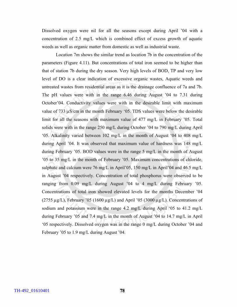
777888

Dissolved oxygen were nil for all the seasons except during April ’04 with a

concentration of 2.5 mg/L which is combined effect of excess growth of aquatic

weeds as well as organic matter from domestic as well as industrial waste.

Location 7m shows the similar trend as location 7b in the concentration of the

parameters (Figure 4.11). But concentrations of total iron seemed to be higher than

that of station 7b during the dry season. Very high levels of BOD, TP and very low

level of DO is a clear indication of excessive organic wastes, Aquatic weeds and

untreated wastes from residential areas as it is the drainage confluence of 7a and 7b.

The pH values were with in the range 6.46 during August ’04 to 7.31 during

October’04. Conductivity values were with in the desirable limit with maximum

value of 733 µS/cm in the month February ‘05. TDS values were below the desirable

limit for all the seasons with maximum value of 477 mg/L in February ’05. Total

solids were with in the range 250 mg/L during October ’04 to 790 mg/L during April

‘05. Alkalinity varied between 102 mg/L in the month of August ‘04 to 408 mg/L

during April ’04. It was observed that maximum value of hardness was 148 mg/L

during February ’05. BOD values were in the range 5 mg/L in the month of August

’05 to 35 mg/L in the month of February ’05. Maximum concentrations of chloride,

sulphate and calcium were 76 mg/L in April’05, 150 mg/L in April’04 and 46.5 mg/L

in August ’04 respectively. Concentration of total phosphorus were observed to be

ranging from 0.09 mg/L during August ’04 to 4 mg/L during February ’05.

Concentrations of total iron showed elevated levels for the months December ’04

(2755 µg/L), February ’05 (1600 µg/L) and April ’05 (3000 µg/L). Concentrations of

sodium and potassium were in the range 4.2 mg/L during April ‘05 to 41.2 mg/L

during February ’05 and 7.4 mg/L in the month of August ’04 to 14.7 mg/L in April

‘05 respectively. Dissolved oxygen was in the range 0 mg/L during October ’04 and

February ’05 to 1.9 mg/L during August ’04.

TH-492_01610401

777999

Location 7m

-1.2

-0.2

0.8

1.8

2.8

3.8

Dec

'03

Apr

'04

Aug

'04

Oct

'04

Dec

'04

Feb'

05

Apr

'05

Stan

dari

zed

valu

e

pH Cond TDS TS Alk hard BO D Cl

Sul Ca TP TI DO MPL

Figure 4.11 Pollution status of location 7m based on standardized value of concentration of different parameters

[[[Cond - conductivity, TDS – total dissolved solids, TS – total solids, Alk – alkalinity, hard – hardness, BOD – biochemical oxygen demand, Cl – chloride, Ca- calcium, TP – total phosphorus, TI – total iron, DO – dissolved oxygen, MPL – maximum permissible level]

TH-492_01610401

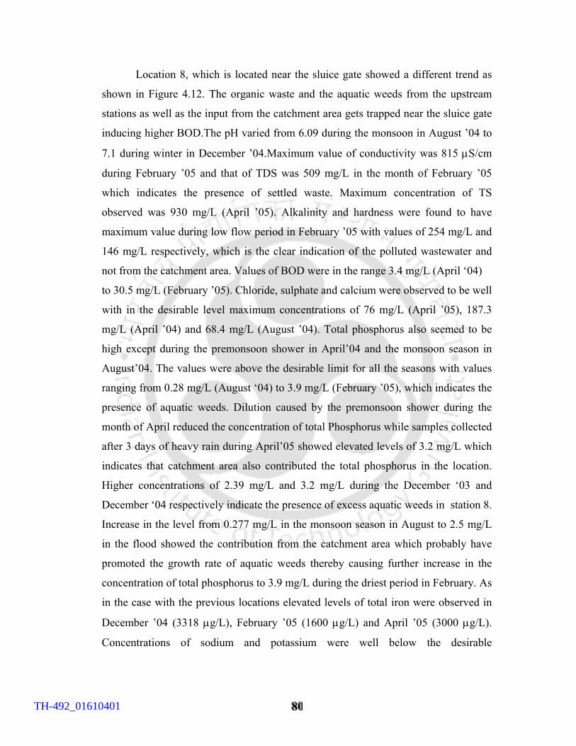
888000

Location 8, which is located near the sluice gate showed a different trend as

shown in Figure 4.12. The organic waste and the aquatic weeds from the upstream

stations as well as the input from the catchment area gets trapped near the sluice gate

inducing higher BOD.The pH varied from 6.09 during the monsoon in August ’04 to

7.1 during winter in December ’04.Maximum value of conductivity was 815 µS/cm

during February ’05 and that of TDS was 509 mg/L in the month of February ’05

which indicates the presence of settled waste. Maximum concentration of TS

observed was 930 mg/L (April ’05). Alkalinity and hardness were found to have

maximum value during low flow period in February ’05 with values of 254 mg/L and

146 mg/L respectively, which is the clear indication of the polluted wastewater and

not from the catchment area. Values of BOD were in the range 3.4 mg/L (April ‘04)

to 30.5 mg/L (February ’05). Chloride, sulphate and calcium were observed to be well

with in the desirable level maximum concentrations of 76 mg/L (April ’05), 187.3

mg/L (April ’04) and 68.4 mg/L (August ’04). Total phosphorus also seemed to be

high except during the premonsoon shower in April’04 and the monsoon season in

August’04. The values were above the desirable limit for all the seasons with values

ranging from 0.28 mg/L (August ‘04) to 3.9 mg/L (February ’05), which indicates the

presence of aquatic weeds. Dilution caused by the premonsoon shower during the

month of April reduced the concentration of total Phosphorus while samples collected

after 3 days of heavy rain during April’05 showed elevated levels of 3.2 mg/L which

indicates that catchment area also contributed the total phosphorus in the location.

Higher concentrations of 2.39 mg/L and 3.2 mg/L during the December ‘03 and

December ‘04 respectively indicate the presence of excess aquatic weeds in station 8.

Increase in the level from 0.277 mg/L in the monsoon season in August to 2.5 mg/L

in the flood showed the contribution from the catchment area which probably have

promoted the growth rate of aquatic weeds thereby causing further increase in the

concentration of total phosphorus to 3.9 mg/L during the driest period in February. As

in the case with the previous locations elevated levels of total iron were observed in

December ’04 (3318 µg/L), February ’05 (1600 µg/L) and April ’05 (3000 µg/L).

Concentrations of sodium and potassium were well below the desirable

TH-492_01610401

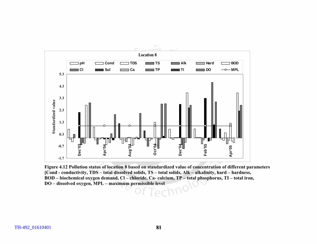
888111

Location 8

-1.7

-0.7

0.3

1.3

2.3

3.3

4.3

5.3D

ec'0

3

Apr

'04

Aug

'04

Oct

'04

Dec

'04

Feb'

05

Apr

'05

Stan

dard

ized

val

ue

pH Cond TDS TS Alk Hard BODCl Sul Ca TP TI DO MPL

Figure 4.12 Pollution status of location 8 based on standardized value of concentration of different parameters

[Cond - conductivity, TDS – total dissolved solids, TS – total solids, Alk – alkalinity, hard – hardness, BOD – biochemical oxygen demand, Cl – chloride, Ca- calcium, TP – total phosphorus, TI – total iron, DO – dissolved oxygen, MPL – maximum permissible level

TH-492_01610401

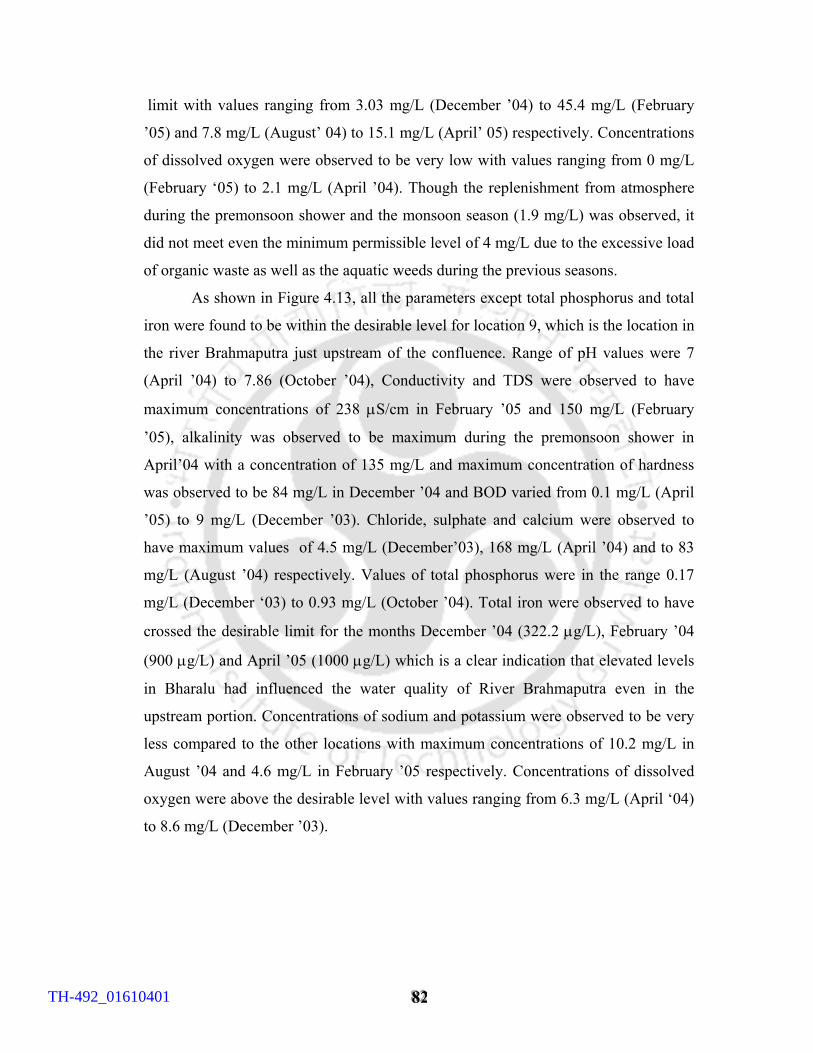
888222

limit with values ranging from 3.03 mg/L (December ’04) to 45.4 mg/L (February

’05) and 7.8 mg/L (August’ 04) to 15.1 mg/L (April’ 05) respectively. Concentrations

of dissolved oxygen were observed to be very low with values ranging from 0 mg/L

(February ‘05) to 2.1 mg/L (April ’04). Though the replenishment from atmosphere

during the premonsoon shower and the monsoon season (1.9 mg/L) was observed, it

did not meet even the minimum permissible level of 4 mg/L due to the excessive load

of organic waste as well as the aquatic weeds during the previous seasons.

As shown in Figure 4.13, all the parameters except total phosphorus and total

iron were found to be within the desirable level for location 9, which is the location in

the river Brahmaputra just upstream of the confluence. Range of pH values were 7

(April ’04) to 7.86 (October ’04), Conductivity and TDS were observed to have

maximum concentrations of 238 µS/cm in February ’05 and 150 mg/L (February

’05), alkalinity was observed to be maximum during the premonsoon shower in

April’04 with a concentration of 135 mg/L and maximum concentration of hardness

was observed to be 84 mg/L in December ’04 and BOD varied from 0.1 mg/L (April

’05) to 9 mg/L (December ’03). Chloride, sulphate and calcium were observed to

have maximum values of 4.5 mg/L (December’03), 168 mg/L (April ’04) and to 83

mg/L (August ’04) respectively. Values of total phosphorus were in the range 0.17

mg/L (December ‘03) to 0.93 mg/L (October ’04). Total iron were observed to have

crossed the desirable limit for the months December ’04 (322.2 µg/L), February ’04

(900 µg/L) and April ’05 (1000 µg/L) which is a clear indication that elevated levels

in Bharalu had influenced the water quality of River Brahmaputra even in the

upstream portion. Concentrations of sodium and potassium were observed to be very

less compared to the other locations with maximum concentrations of 10.2 mg/L in

August ’04 and 4.6 mg/L in February ’05 respectively. Concentrations of dissolved

oxygen were above the desirable level with values ranging from 6.3 mg/L (April ‘04)

to 8.6 mg/L (December ’03).

TH-492_01610401

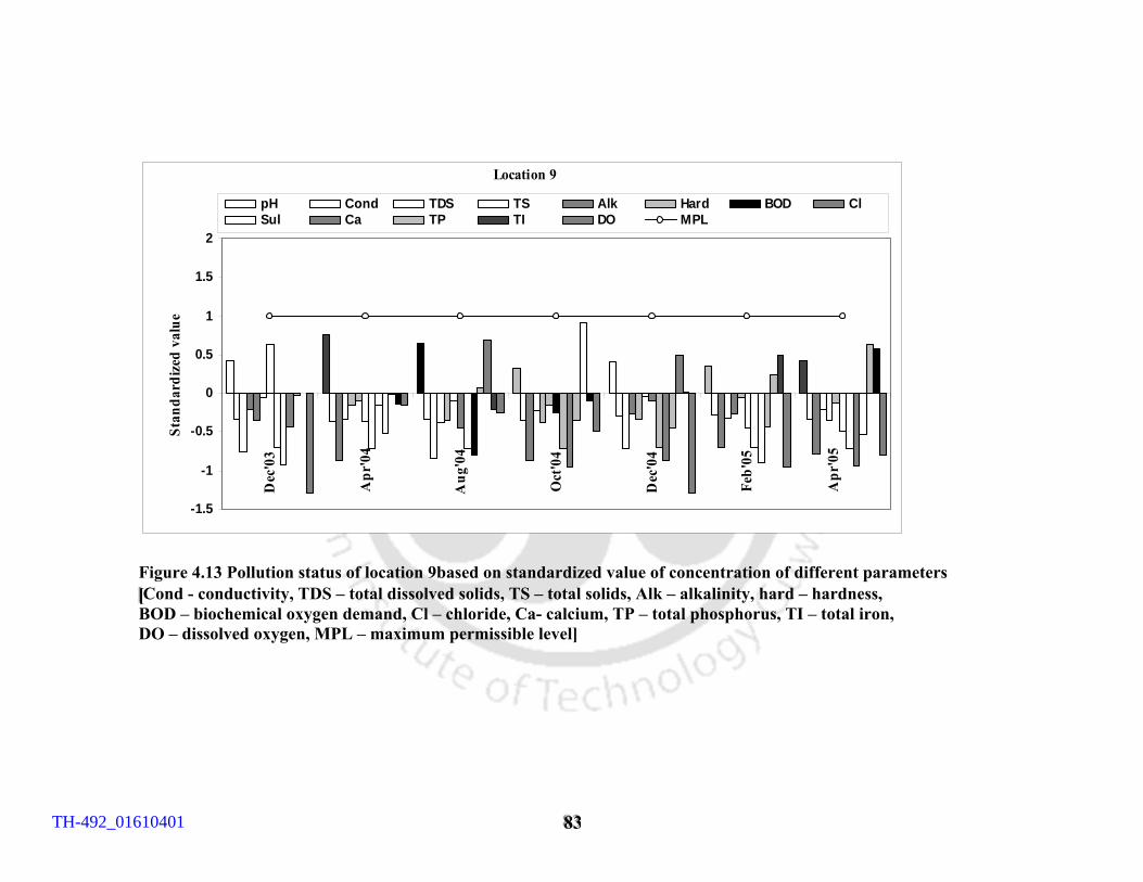
888333

Location 9

-1.5

-1

-0.5

0

0.5

1

1.5

2

Dec

'03

Apr

'04

Aug

'04

Oct

'04

Dec

'04

Feb'

05

Apr

'05

Stan

dard

ized

val

ue

pH Cond TDS TS Alk Hard BOD ClSul Ca TP TI DO MPL

Figure 4.13 Pollution status of location 9based on standardized value of concentration of different parameters [[[Cond - conductivity, TDS – total dissolved solids, TS – total solids, Alk – alkalinity, hard – hardness, BOD – biochemical oxygen demand, Cl – chloride, Ca- calcium, TP – total phosphorus, TI – total iron, DO – dissolved oxygen, MPL – maximum permissible level]

TH-492_01610401

888444

Location 10 is the point on river Bharalu just before it meets River Brahmaputra

near Bharalumukh .pH varied between 6.14 during August ’04 and 7.26 during October

’04 (Figure 4.14). Maximum value of conductivity was within the desirable level with a

value of 733 µS/cm in the month of February ’05. TDS and TS were in the range 208

mg/L (October ’04) to 470.6 mg/L (December ’04) and 248 mg/L (October ’04) to 520

mg/L (December ‘03) respectively. Elevated levels during the low flow periods indicate

the dissolved as well as suspended solids carried down from the upstream as well as the

subsurface flow. Alkalinity values were higher than the desirable range with maximum

value during April ’04 (375 mg/L). Hardness was maximum in April’ 04 (154 mg/L).

This indicates that alkalinity and hardness were induced by the run off through the

catchment. BOD were below the desirable value during April ’04 with a value of 1.9

mg/L and for all other seasons values were above the desirable level with a maximum

value of 32 mg/L during February ’05 which indicates the settled organic waste.

Maximum concentrations of Chloride, sulphate and calcium were observed to be 50 mg/L

(February ’05), 261 mg/L (April ’04) and 54 mg/L (August ’04) respectively. Chloride in

comparatively higher concentration confirms the presence of settled wastes. All values

were with in the desirable limit except for sulphate during April’04 and refuse leachates

carried down by the surface run off could be the probable cause. Concentrations of total

phosphorus and total iron varied from 0.04 mg/L (April ‘04) to 1.622 mg/L (October ’04)

and 0.83 µg/L (August ’04) to 4607.8 µg/L (December ’04) respectively. Elevated levels

of total phosphorus indicate the excess growth of aquatic weeds in the location and that

of total iron in the dry season is the clear indication that subsurface flow is prominent.

Sodium and potassium were very low for all the seasons with maximum concentrations

of 48.9 mg/L (February ’05) and 12.8 mg/L (April ’05) respectively. Dissolved oxygen is

very low with values ranging from 0 mg/L (February ’05) to 2 mg/L (August ’04) which

is the indication of excess aquatic weeds as well as organic wastes due to the pollution

from land as well as water.

TH-492_01610401

888555

Location 10

-1

-0.5

0

0.5

1

1.5

Dec

'03

Apr

'04

Aug

'04

Oct

'04

Dec

'04

Feb'

05

Apr

'05

Stan

dard

ized

val

ue

pH Cond TDS TS Alkn Hard BODCl Sulphate Ca TP TI DO MPL


TH-492_01610401

888666

Location 11 is the location on River Brahmaputra about 1.5 kms down stream of

the confluence. Sampling of this location was carried out to check whether there is any

change in the quality compared to that of the location 9 of river Brahmaputra. pH values

were in the range 6.44 (April ‘04) to 7.4 (February ’05), which is slightly less than that of

location 9. Slight Increase in all other parameters was observed for this location (Figure

4.15). Conductivities were observed to have a maximum concentration of 306 µS/cm

(October ’04). TDS also showed the same trend with maximum concentration of 198

mg/L (October ’04). Higher levels of dissolved salts in the post monsoon season indicate

presence of settled wastes brought down to the river from the tributary during the

monsoon season. Maximum values of alkalinity and hardness observed were 153 mg/L

(April ’04) and 86 mg/L (December ’04) respectively that are with in the desirable levels.

Elevated levels of alkalinity during the pre monsoon shower indicate the contribution

from the adjoining land and subsurface flow and waste from the tributary is the probable

source of hardness during the dry period. Maximum value of BOD (11.33 mg/L) during

the winter season in December ’03 indicates the presence of settled organic waste.

Chloride, sulphate and calcium were observed to have maximum concentration of 15.5

mg/L (October ’04), 161.3 mg/L (April ’04) and 51.6 mg/L (August ’04) respectively.

Concentrations of total phosphorus varied from 0.03 mg/L (April ‘04) to 1.348 mg/L

(October ’04) and that of total iron was in the range 0 µg/L (August ‘04) to 1800 µg/L

(April ’05). These observations show that the pollutants were carried down from the

polluted tributary to the main river. Sodium and potassium were observed to have

maximum concentrations of 12.7 mg/L (October ’04) 6.1 mg/L (August ’04),

respectively. Decline in dissolved oxygen was also observed for this location with

concentration ranging from 3.6 mg/L (December ’03) to 7.3 mg/L (December ’04).

TH-492_01610401

888777

Location 11

-1

-0.5

0

0.5

1

1.5

2

Dec

'03

Apr

'04

Aug

'04

Oct

'04

Dec

'04

Feb'

05

Apr

'05

Stan

ariz

ed v

alue

pH Cond TDS TS Alk Hard BOD Cl SulCa TP TI DO MPL

Figure 4.15 Pollution status of location 11 based on standardized value of concentration of different parameters [Cond - conductivity, TDS – total dissolved solids, TS – total solids, Alk – alkalinity, hard – hardness,

BOD – biochemical oxygen demand, cl – chloride, Ca- calcium, TP – total phosphorus, TI – total iron, DO – dissolved oxygen, MPL – maximum permissible level].

TH-492_01610401

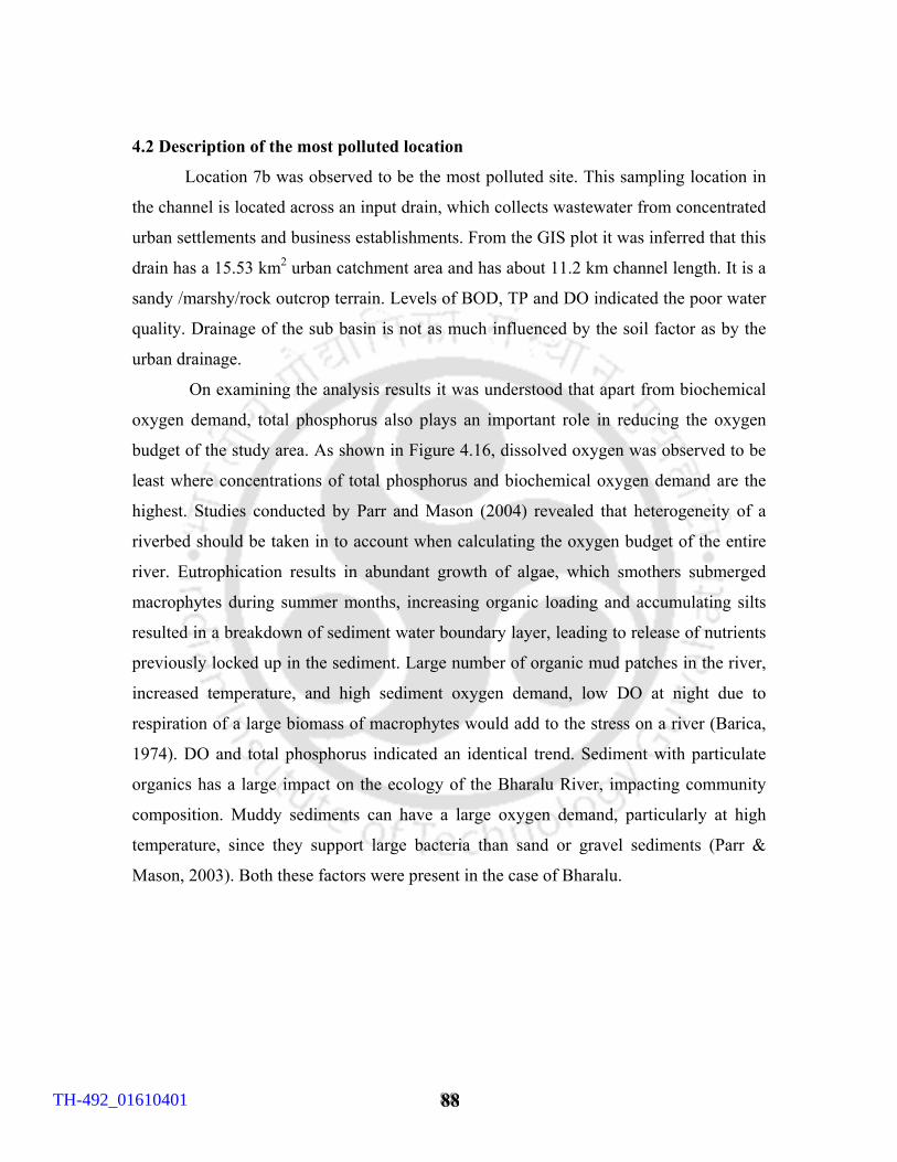
888888

4.2 Description of the most polluted location

Location 7b was observed to be the most polluted site. This sampling location in

the channel is located across an input drain, which collects wastewater from concentrated

urban settlements and business establishments. From the GIS plot it was inferred that this

drain has a 15.53 km2 urban catchment area and has about 11.2 km channel length. It is a

sandy /marshy/rock outcrop terrain. Levels of BOD, TP and DO indicated the poor water

quality. Drainage of the sub basin is not as much influenced by the soil factor as by the

urban drainage.

On examining the analysis results it was understood that apart from biochemical

oxygen demand, total phosphorus also plays an important role in reducing the oxygen

budget of the study area. As shown in Figure 4.16, dissolved oxygen was observed to be

least where concentrations of total phosphorus and biochemical oxygen demand are the

highest. Studies conducted by Parr and Mason (2004) revealed that heterogeneity of a

riverbed should be taken in to account when calculating the oxygen budget of the entire

river. Eutrophication results in abundant growth of algae, which smothers submerged

macrophytes during summer months, increasing organic loading and accumulating silts

resulted in a breakdown of sediment water boundary layer, leading to release of nutrients

previously locked up in the sediment. Large number of organic mud patches in the river,

increased temperature, and high sediment oxygen demand, low DO at night due to

respiration of a large biomass of macrophytes would add to the stress on a river (Barica,

1974). DO and total phosphorus indicated an identical trend. Sediment with particulate

organics has a large impact on the ecology of the Bharalu River, impacting community

composition. Muddy sediments can have a large oxygen demand, particularly at high

temperature, since they support large bacteria than sand or gravel sediments (Parr &

Mason, 2003). Both these factors were present in the case of Bharalu.

TH-492_01610401

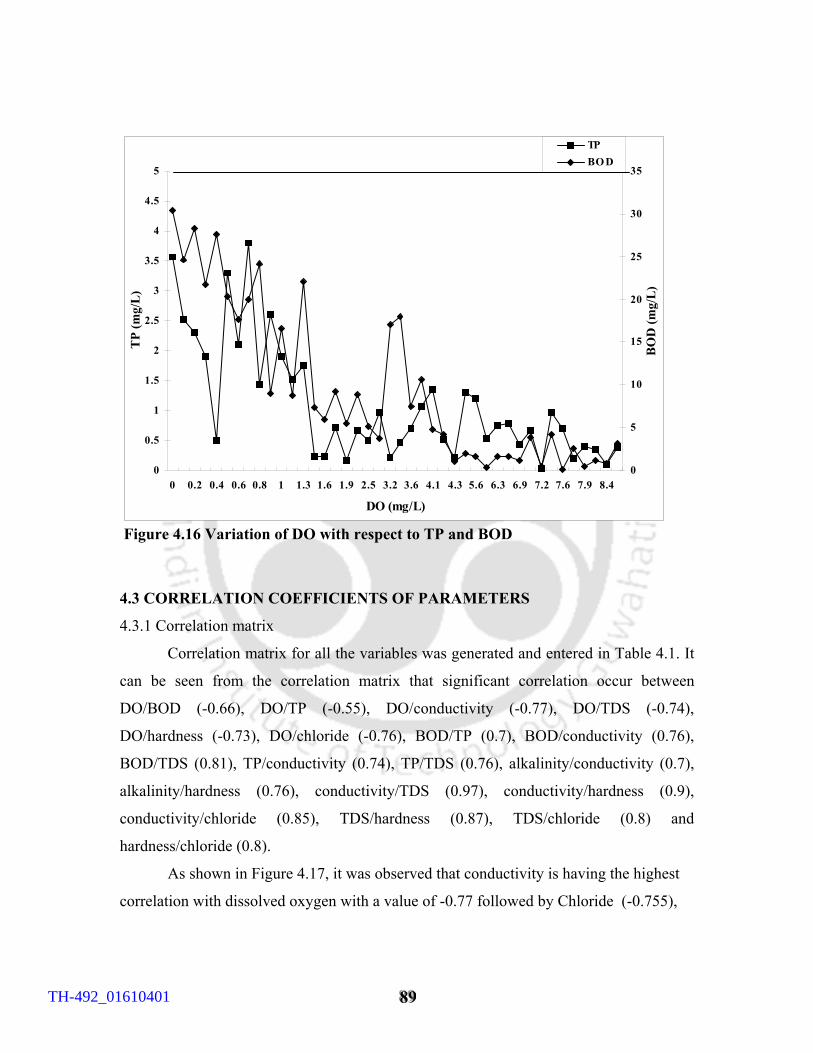
888999

Figure 4.16 Variation of DO with respect to TP and BOD

4.3 CORRELATION COEFFICIENTS OF PARAMETERS

4.3.1 Correlation matrix

Correlation matrix for all the variables was generated and entered in Table 4.1. It

can be seen from the correlation matrix that significant correlation occur between

DO/BOD (-0.66), DO/TP (-0.55), DO/conductivity (-0.77), DO/TDS (-0.74),

DO/hardness (-0.73), DO/chloride (-0.76), BOD/TP (0.7), BOD/conductivity (0.76),

BOD/TDS (0.81), TP/conductivity (0.74), TP/TDS (0.76), alkalinity/conductivity (0.7),

alkalinity/hardness (0.76), conductivity/TDS (0.97), conductivity/hardness (0.9),

conductivity/chloride (0.85), TDS/hardness (0.87), TDS/chloride (0.8) and

hardness/chloride (0.8).

As shown in Figure 4.17, it was observed that conductivity is having the highest

correlation with dissolved oxygen with a value of -0.77 followed by Chloride (-0.755),

0

0.5

1

1.5

2

2.5

3

3.5

4

4.5

5

0 0.2 0.4 0.6 0.8 1 1.3 1.6 1.9 2.5 3.2 3.6 4.1 4.3 5.6 6.3 6.9 7.2 7.6 7.9 8.4

DO (mg/L)

TP

(mg/

L)

0

5

10

15

20

25

30

35

BO

D (m

g/L

)

TPBO D

TH-492_01610401

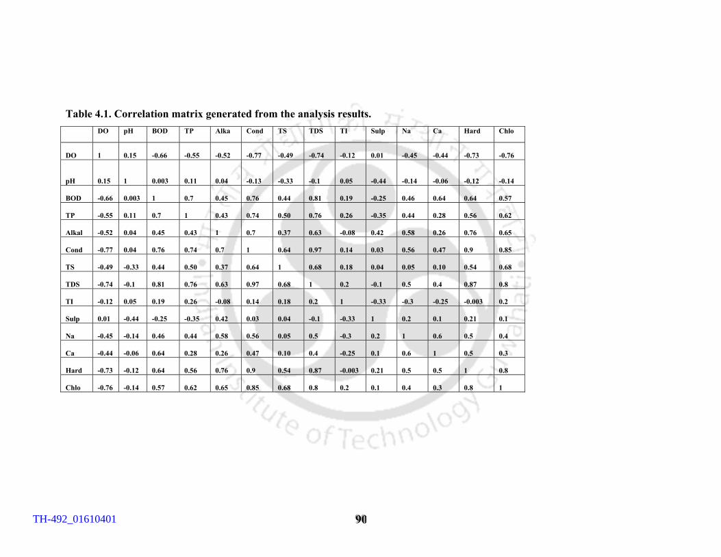
999000

Table 4.1. Correlation matrix generated from the analysis results. DO pH BOD TP Alka Cond TS TDS TI Sulp Na Ca Hard Chlo

DO

1

0.15

-0.66

-0.55

-0.52

-0.77

-0.49

-0.74

-0.12

0.01

-0.45

-0.44

-0.73

-0.76

pH

0.15

1

0.003

0.11

0.04 -0.13 -0.33 -0.1 0.05 -0.44 -0.14 -0.06 -0.12 -0.14

BOD

-0.66

0.003

1 0.7 0.45 0.76 0.44 0.81 0.19 -0.25 0.46 0.64 0.64 0.57

TP

-0.55

0.11

0.7 1 0.43 0.74 0.50 0.76 0.26 -0.35 0.44 0.28 0.56 0.62

Alkal

-0.52

0.04

0.45 0.43

1 0.7 0.37 0.63 -0.08 0.42 0.58 0.26 0.76 0.65

Cond

-0.77

0.04

0.76 0.74 0.7 1 0.64 0.97 0.14 0.03 0.56 0.47 0.9 0.85

TS

-0.49

-0.33

0.44 0.50 0.37 0.64 1 0.68 0.18 0.04 0.05 0.10 0.54 0.68

TDS

-0.74

-0.1

0.81 0.76 0.63 0.97 0.68 1 0.2 -0.1 0.5 0.4 0.87 0.8

TI

-0.12

0.05

0.19 0.26 -0.08 0.14 0.18 0.2 1 -0.33 -0.3 -0.25 -0.003 0.2

Sulp

0.01

-0.44

-0.25 -0.35 0.42 0.03 0.04 -0.1 -0.33 1 0.2 0.1 0.21 0.1

Na

-0.45

-0.14

0.46 0.44 0.58 0.56 0.05 0.5 -0.3 0.2 1 0.6 0.5 0.4

Ca

-0.44

-0.06

0.64 0.28 0.26 0.47 0.10 0.4 -0.25 0.1 0.6 1 0.5 0.3

Hard

-0.73

-0.12

0.64 0.56

0.76 0.9 0.54 0.87 -0.003 0.21 0.5 0.5 1 0.8

Chlo

-0.76

-0.14

0.57 0.62 0.65 0.85 0.68 0.8 0.2 0.1 0.4 0.3 0.8 1

TH-492_01610401

999111

total dissolved solids (-0.735), hardness (-0.731), potassium (-0.663), bio chemical

oxygen demand (-0.656), total phosphorus (-0.554), alkalinity (-0.552), total solids (-

0.486), sodium (-0.445), calcium (-0.435), pH (0.152), sulphate (0.013). Negative value

for a parameter indicates that dissolved oxygen decreases with increase in concentration

of that particular parameter and positive value indicates that dissolved oxygen increases

with increase in the concentration of the parameter. Here all the parameters except pH

and sulphate showed negative correlation.

-1

-0.8

-0.6

-0.4

-0.2

0

0.2

pH

B O

D T P

Alk

alin

ity

Con

duct

ivity T S

T D

S TI

Sulp

hate

Pota

ssiu

m

Sodi

um

Cal

cium

Har

dnes

s

Chl

orid

eParameter

Cor

rela

tion

coef

ficie

nt

Figure 4.17. Correlation coefficients of parameters with respect to dissolved oxygen

The graphical representation of average concentrations of parameters with

comparatively higher correlation (above 50%) with dissolved oxygen is shown in Figure

4.18. All the sampling stations except the origin at Basista and the location at River

Brahmaputra were highly contaminated in terms of biochemical oxygen demand, total phosphorus and dissolved oxygen biochemical oxygen demand, total phosphorus,

TH-492_01610401

999222

alkalinity, conductivity, total dissolved solids, potassium, hardness and chloride are

having comparatively higher correlation coefficient (above 50%). Average concentrations

of BOD varied from 3.9 mg/L to 31 mg/L, total phosphorus varied from 0.62 mg/L to

5.16 mg/L, alkalinity varied from 37.2 mg/L to 354 mg/L, conductivity varied from 63.3

µS/cm to 982 µS/cm, total dissolved solids from 36.5 mg/L to 587 mg/L, potassium from

2.7 mg/L to 16.7 mg/L, hardness from 17 mg/L to 169 mg/L and chloride from 1.8 mg/L

to 64.4 mg/L. Among these parameters, the concentrations of potassium, hardness and

chloride are well below the permissible limits of 100 mg/L, 500 mg/L, and 600 mg/L and

even below the desirable limits of 100 mg/L, 200 mg/L and 200 mg/L, respectively.

Concentration of total dissolved solids is well below the maximum permissible limit of

1500 mg/L but it was observed to be above the desirable level of 500 mg/L during the dry

season. Maximum average value of conductivity was found to be above the desirable

limit but concentrations were well below the maximum permissible limit of 2500 µS/cm.

Same trend was observed for alkalinity also. Concentrations of biochemical oxygen

demand as well as total phosphorus were observed to be very high. Dissolved oxygen

was observed to be well below the maximum allowable level of 4 mg/L with average

concentrations ranging from 0.34 mg/L to 7.7 mg/L. High level of biochemical oxygen

demand as well as total phosphorus and low DO is the clear indication of excess quantity

of organic wastes as well as aquatic weeds.

Chloride is found in most natural waters and is not of concern at low levels.

Analysis results revealed that maximum concentration of chloride was 92 mg/L that is

well below the desirable limit of 250 mg/L that was observed at 7b, the most

contaminated location. Chloride ions (Cl-) contribute to total salt content (electrical

conductivity) of the water, which is also evident from the high correlation (0.85) between

conductivity and chloride. Hardness is a measure of the amount of calcium, magnesium,

and iron dissolved in water. Hardness showed strong correlations with alkalinity (0.76),

conductivity (0.9) and total dissolved solids (0.87).

TH-492_01610401

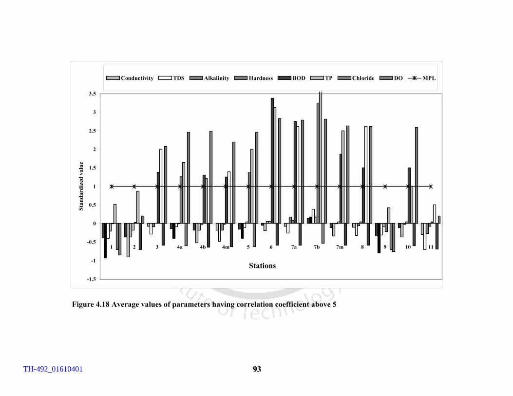
999333

-1.5

-1

-0.5

0

0.5

1

1.5

2

2.5

3

3.5

1 2 3 4a 4b 4m 5 6 7a 7b 7m 8 9 10 11

Stations

Stan

dard

ized

val

ueConductivity TDS Alkalinity Hardness BOD TP Chloride DO MPL

Figure 4.18 Average values of parameters having correlation coefficient above 5

TH-492_01610401

999444

4.4 CONCLUSIONS

For the Bharalu catchment and the stream, the water quality was found to be

generally poor, with significant seasonal and spatial variations. Dissolved oxygen, which

is a major water quality indicator, was observed to be either absent or very low in several

locations irrespective of the season. Following conclusions can be drawn based on the

water quality evaluation.

• Urban runoff was observed to have predominant influence on alkalinity.

Maximum values of alkalinity were observed in all locations during the

premonsoon shower. Maximum value of 592 mg/L was observed in location 7a

with catchment area of 40 km2, which covers agricultural land, residential

complexes and a large medical campus. The premonsoon shower after a after a

long spell of dry season was observed to increase the alkalinity which could be

due to the contribution from the catchment area. But this increase in value is only

for a short period as the observation obtained from the samples collected during

the monsoon season indicated reduction in alkalinity due to dilution.

• Elevated levels of conductivity during the low flow period indicate the presence

of subsurface flow in the middle reaches. Higher levels in the points of origin

during premonsoon shower indicate the contribution from the catchment area,

which is free from human interference.

• No significant seasonal variation was observed for chloride concentration.

Increasing concentration towards the down stream is a clear indication of

increasing pollution and comparatively higher concentration during the low flow

period indicates the wastes getting concentrated due to lack of dilution as well as

the presence of ion rich subsurface flow which is the case for conductivity also.

• Concentrations of sulphate showed pronounced seasonal variation, and elevated

levels in the wet season indicate land use pattern plays a major role in sulphate

concentration irrespective of the catchment area. This is evident from the

observation in station 7b.

• Total phosphorus was high in all the locations promoting excessive growth of

weeds and inducing more stress on DO of the water channel. Very high

concentration of TP indicates the decayed organic waste in the bed apart from excess

TH-492_01610401

999555

growth of aquatic weeds which results in release of nutrients from the sediment water

interface

• Combined effect of total phosphorus and organic matter brought down the DO

well below the permissible level. The drains from the urban area and the market

place carried dead water without any dissolved oxygen at all.

• BOD and total phosphorus were found to be the crucial parameters to be managed

to improve the quality of the system studied.

• The locations in the middle reaches, especially location 7b, were the most affected

location due to expanding urban growth. This underlines the need of a proper

waste management scheme for the whole city and that of a treatment plant before

the wastewater of the Bharalu tributary is discharged into the river Brahmaputra.

TH-492_01610401

999666

CHAPTER FIVE MODELING METHODOLOGY 5.1 INPUT AND OUTPUT VARIABLES

One of the main causes of oxygen depletion or sinks is the oxidation of organic

matter and other reduced matter in the water column (Cox, 2003). Hence BOD was taken

as one of the input parameters for modeling. Phosphorus and nitrogen are nutrients,

which are most important for the growth of blue green algae that imparts discoloration,

odor, and formation of unsightly, smelly scums on the water surface (Maier & Dandy,

1997). These were exactly the characteristics of the study area. Of the two nutrients

nitrogen and phosphorus, phosphorus is regarded as the limiting nutrient. When there is

too much phosphorus in water, eutrophication can be speeded up that result in depletion

in dissolved oxygen. Phosphorus gets into water in both urban and agricultural settings

and it tends to attach to soil particles and thus moves into surface water bodies from run

off. Rapid growth of aquatic vegetation as a result of excess phosphorus lowers the

dissolved oxygen as the vegetation dies and decays and uses up oxygen. Considering this

fact and comparatively higher correlation coefficient obtained from the data generated

from laboratory analysis, it was decided to take total phosphorus as the second input

parameter. Experimental data showed that conductivity showed highest correlation with

dissolved oxygen. Electrical conductivity estimates the amount of total dissolved salts.

Bacterial metabolism in the nutrient rich river bed consumes oxygen and release

CO2.This CO2 rapidly dissolves in water to form carbonic acid, bicarbonate ions and

carbonate ions and the new ions increase the TDS and therefore the conductivity. Hence

increase in conductivity can also be correlated to dissolved oxygen depletion. Hence it

was selected as the third input parameter. Alkalinity was included as the fourth input

parameter to simulate the chemical properties of the habitat. The input and output

parameters are given in Table 5.1 with their minimum and maximum values.

TH-492_01610401

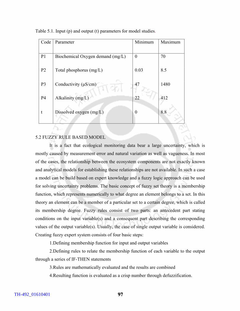
999777

Table 5.1. Input (p) and output (t) parameters for model studies.

Code Parameter Minimum Maximum

P1 Biochemical Oxygen demand (mg/L) 0 70

P2 Total phosphorus (mg/L) 0.03 8.5

P3 Conductivity (µS/cm) 47 1480

P4 Alkalinity (mg/L) 22 412

t Dissolved oxygen (mg/L) 0 8.8

5.2 FUZZY RULE BASED MODEL

It is a fact that ecological monitoring data bear a large uncertainty, which is

mostly caused by measurement error and natural variation as well as vagueness. In most

of the cases, the relationship between the ecosystem components are not exactly known

and analytical models for establishing these relationships are not available. In such a case

a model can be build based on expert knowledge and a fuzzy logic approach can be used

for solving uncertainty problems. The basic concept of fuzzy set theory is a membership

function, which represents numerically to what degree an element belongs to a set. In this

theory an element can be a member of a particular set to a certain degree, which is called

its membership degree. Fuzzy rules consist of two parts: an antecedent part stating

conditions on the input variable(s) and a consequent part describing the corresponding

values of the output variable(s). Usually, the case of single output variable is considered.

Creating fuzzy expert system consists of four basic steps:

1.Defining membership function for input and output variables

2.Defining rules to relate the membership function of each variable to the output

through a series of IF-THEN statements

3.Rules are mathematically evaluated and the results are combined

4.Resulting function is evaluated as a crisp number through defuzzification.

TH-492_01610401

999888

On examining the generated data, the domain of each input variable was

partitioned into number of fuzzy sets or linguistic variables. A fuzzy rule base system

was constructed that connects the input variables to the output variable by means of IF-

THEN rules. Given particular values of the input variables degree of fulfillment of the

rule is obtained by aggregating the membership degrees of these input values into the

respective fuzzy sets. Fuzzy output was determined by the degrees of fulfillment and the

consequent parts of the rules. In this study the famous Mamdani method with the help of

math work’s MATLAB fuzzy logic toolbox editor (version 6.0.0.88 Release 12) was used

to develop the prediction model. According to this method, being the kth crisp input

variable defined as ak, Ai, j, k, its corresponding jth fuzzy input number considered in the ith

rule Bi,l is the lth fuzzy output number relevant to the ith rule , the Mamdani rule is

IF a1 is A i,j,1 AND a2 is A i,j,2 AND...AND aK is A i,j,k THEN B i,l

Fuzzy operator ‘minimum’ was applied as the variables are combined using ‘AND’ and

the aggregation was performed with the ‘maximum’ function. The centrioid or center of

gravity method was applied as a means of defuzzification of the output membership

function to determine a crisp set.

5.2.1 DESCRIPTION OF FUZZY REGIONS

Based on the correlation coefficients four sensitive parameters namely the

biochemical oxygen demand (BOD), total phosphorus (TP), conductivity and alkalinity

were selected as the input variables and dissolved oxygen as the output variables. Taking

the experimental data into consideration these parameters were fuzzified into fuzzy

subsets as shown in Tables 5.2 to 5.6 and Figures 5.1 to 5.5. Membership functions of

input and output variables were created using fuzzy logic tool box editor.

Trapizoidal fuzzy number A is defined by the membership function

TH-492_01610401

999999

1

11

1

aaax−

− for a1 ≤ x ≤ 1

1a

µ = 1 for a11 ≤ x ≤ a 1

2

2

12

2

aa

ax

−

− for a1

2 ≤ x ≤ a2

0 Otherwise,

Where [a1, a2] is the supporting interval and 11a and a1

2 are the values at the highest

level of the trapezoidal region.

11a a 1

2

a1 x a2

Triangular fuzzy number A is defined by the membership function aM

1

1aa

ax

M −−

for a1 ≤ x ≤ Ma a a aM M aaa

µ = 2

2aa

ax

M −−

for aM ≤ x ≤ 2a µ

000 otherwise

aaa111 a2

TH-492_01610401

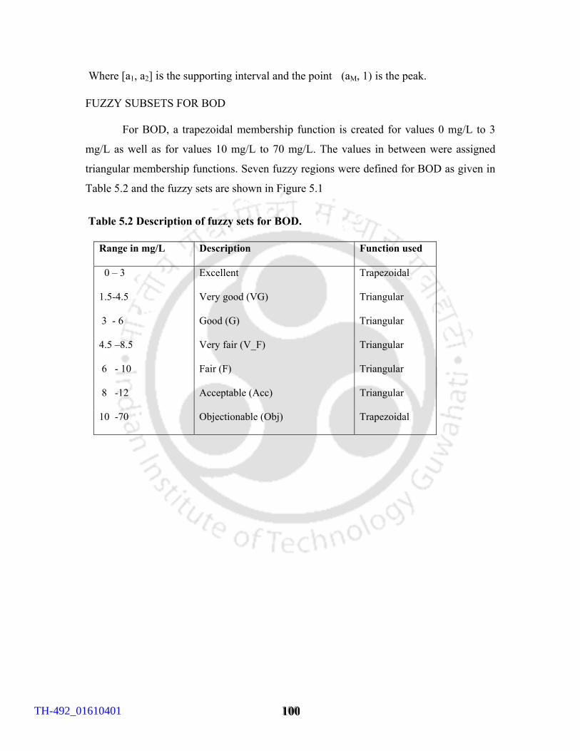
111000000

Where [a1, a2] is the supporting interval and the point (aM, 1) is the peak.

FUZZY SUBSETS FOR BOD

For BOD, a trapezoidal membership function is created for values 0 mg/L to 3

mg/L as well as for values 10 mg/L to 70 mg/L. The values in between were assigned

triangular membership functions. Seven fuzzy regions were defined for BOD as given in

Table 5.2 and the fuzzy sets are shown in Figure 5.1

Table 5.2 Description of fuzzy sets for BOD.

Range in mg/L Description Function used

0 – 3 Excellent Trapezoidal

1.5-4.5 Very good (VG)

Triangular

3 - 6 Good (G) Triangular

4.5 –8.5 Very fair (V_F)

Triangular

6 - 10 Fair (F) Triangular

8 -12 Acceptable (Acc) Triangular

10 -70 Objectionable (Obj)

Trapezoidal

TH-492_01610401

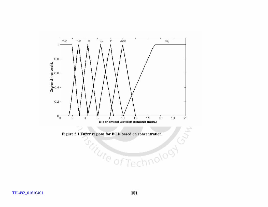
111000111

Figure 5.1 Fuzzy regions for BOD based on concentration

TH-492_01610401

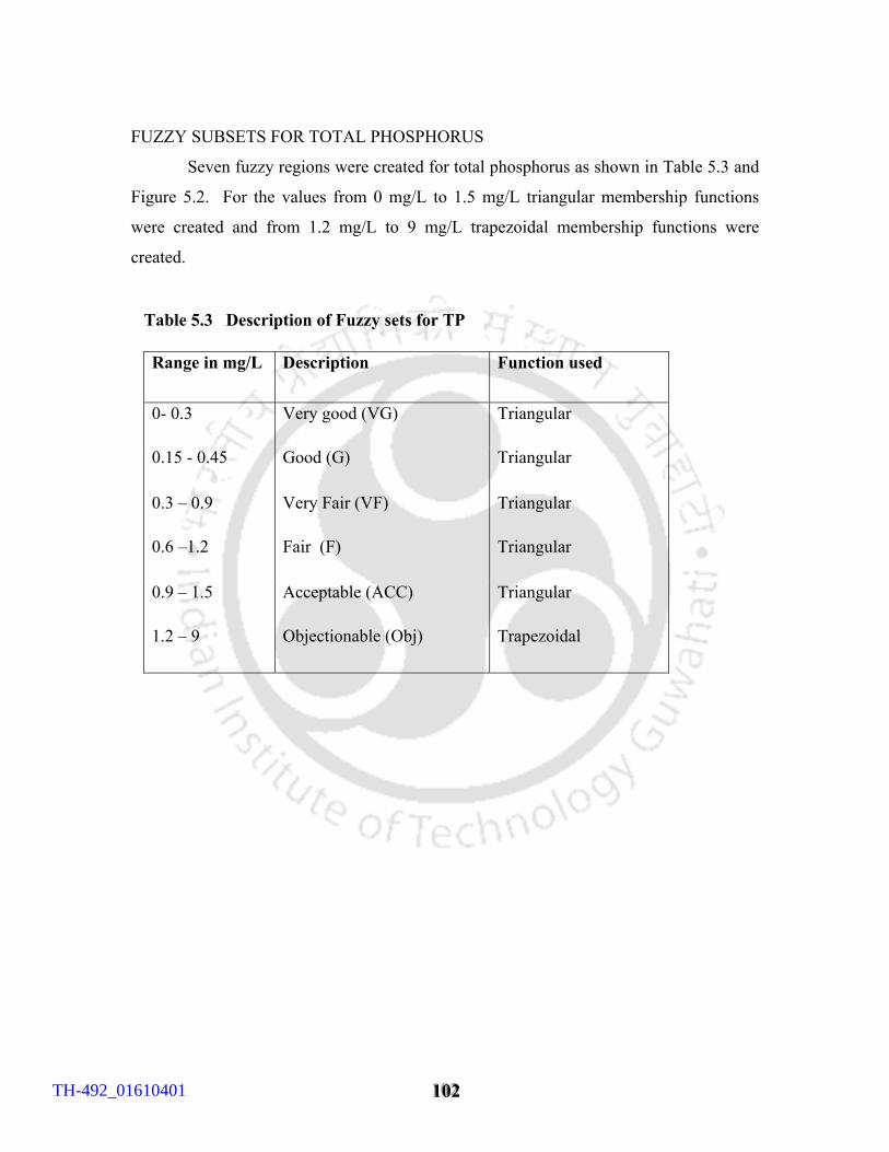
111000222

FUZZY SUBSETS FOR TOTAL PHOSPHORUS

Seven fuzzy regions were created for total phosphorus as shown in Table 5.3 and

Figure 5.2. For the values from 0 mg/L to 1.5 mg/L triangular membership functions

were created and from 1.2 mg/L to 9 mg/L trapezoidal membership functions were

created.

Table 5.3 Description of Fuzzy sets for TP


0- 0.3 Very good (VG) Triangular

0.15 - 0.45 Good (G) Triangular

0.3 – 0.9 Very Fair (VF) Triangular

0.6 –1.2 Fair (F) Triangular

0.9 – 1.5 Acceptable (ACC) Triangular

1.2 – 9 Objectionable (Obj) Trapezoidal

TH-492_01610401

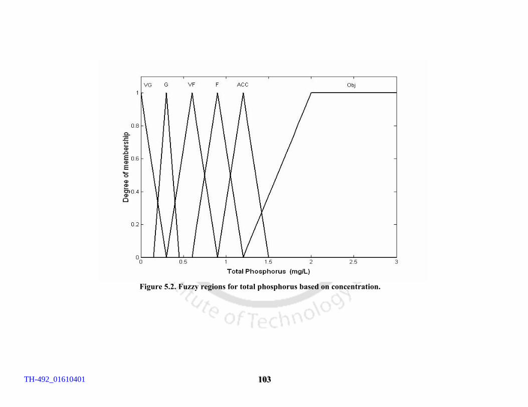
111000333

Figure 5.2. Fuzzy regions for total phosphorus based on concentration.

TH-492_01610401

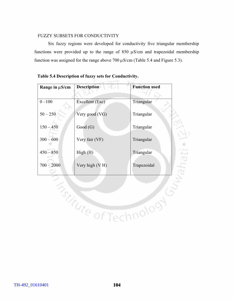
111000444

FUZZY SUBSETS FOR CONDUCTIVITY

Six fuzzy regions were developed for conductivity five triangular membership

functions were provided up to the range of 850 µS/cm and trapezoidal membership

function was assigned for the range above 700 µS/cm (Table 5.4 and Figure 5.3).

Table 5.4 Description of fuzzy sets for Conductivity.

Range in µS/cm Description Function used

0 –100 Excellent (Exc) Triangular

50 – 250 Very good (VG) Triangular

150 – 450 Good (G) Triangular

300 – 600 Very fair (VF) Triangular

450 – 850 High (H) Triangular

700 – 2000 Very high (V H) Trapezoidal

TH-492_01610401

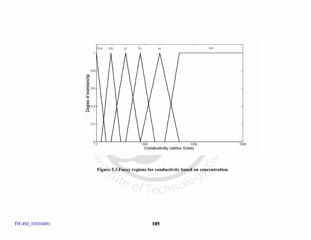
111000555

Figure 5.3.Fuzzy regions for conductivity based on concentration.

TH-492_01610401

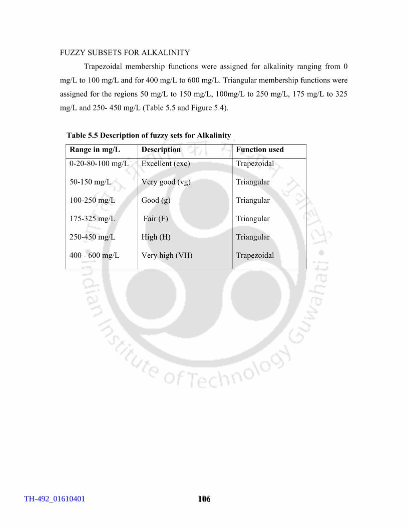
111000666

FUZZY SUBSETS FOR ALKALINITY

Trapezoidal membership functions were assigned for alkalinity ranging from 0

mg/L to 100 mg/L and for 400 mg/L to 600 mg/L. Triangular membership functions were

assigned for the regions 50 mg/L to 150 mg/L, 100mg/L to 250 mg/L, 175 mg/L to 325

mg/L and 250- 450 mg/L (Table 5.5 and Figure 5.4).

Table 5.5 Description of fuzzy sets for Alkalinity


0-20-80-100 mg/L Excellent (exc) Trapezoidal

50-150 mg/L Very good (vg) Triangular

100-250 mg/L Good (g) Triangular

175-325 mg/L Fair (F) Triangular

250-450 mg/L High (H) Triangular

400 - 600 mg/L Very high (VH) Trapezoidal

TH-492_01610401

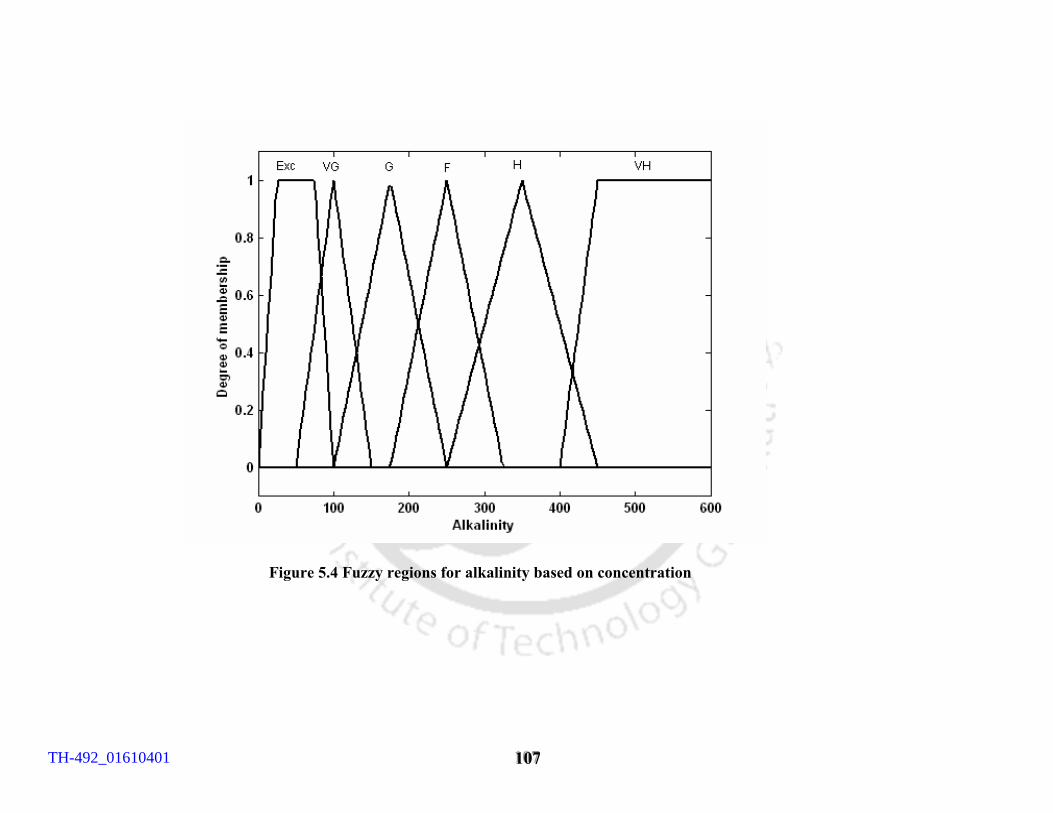
111000777

Figure 5.4 Fuzzy regions for alkalinity based on concentration

TH-492_01610401

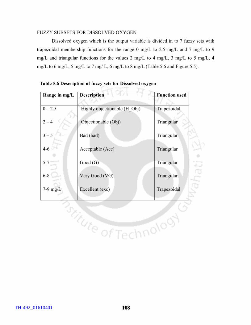
111000888

FUZZY SUBSETS FOR DISSOLVED OXYGEN

Dissolved oxygen which is the output variable is divided in to 7 fuzzy sets with

trapezoidal membership functions for the range 0 mg/L to 2.5 mg/L and 7 mg/L to 9

mg/L and triangular functions for the values 2 mg/L to 4 mg/L, 3 mg/L to 5 mg/L, 4

mg/L to 6 mg/L, 5 mg/L to 7 mg/ L, 6 mg/L to 8 mg/L (Table 5.6 and Figure 5.5).

Table 5.6 Description of fuzzy sets for Dissolved oxygen


0 – 2.5 Highly objectionable (H_Obj) Trapezoidal

2 – 4 Objectionable (Obj) Triangular

3 – 5 Bad (bad) Triangular

4-6 Acceptable (Acc) Triangular

5-7 Good (G) Triangular

6-8 Very Good (VG) Triangular

7-9 mg/L Excellent (exc) Trapezoidal

TH-492_01610401

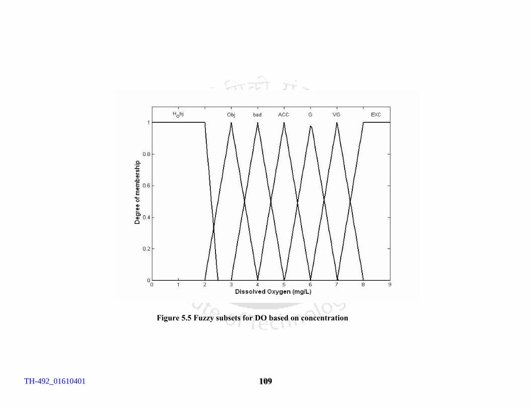
111000999

Figure 5.5 Fuzzy subsets for DO based on concentration

TH-492_01610401

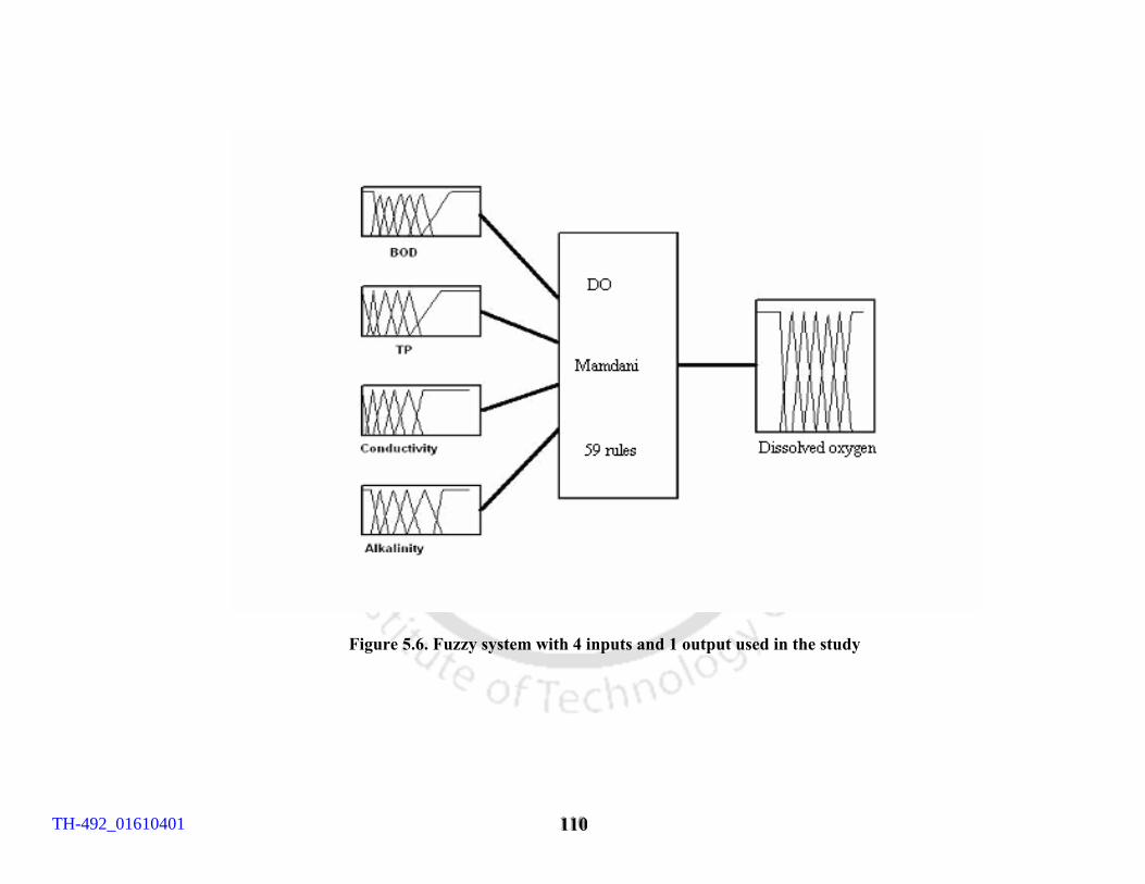
111111000

Figure 5.6. Fuzzy system with 4 inputs and 1 output used in the study

TH-492_01610401

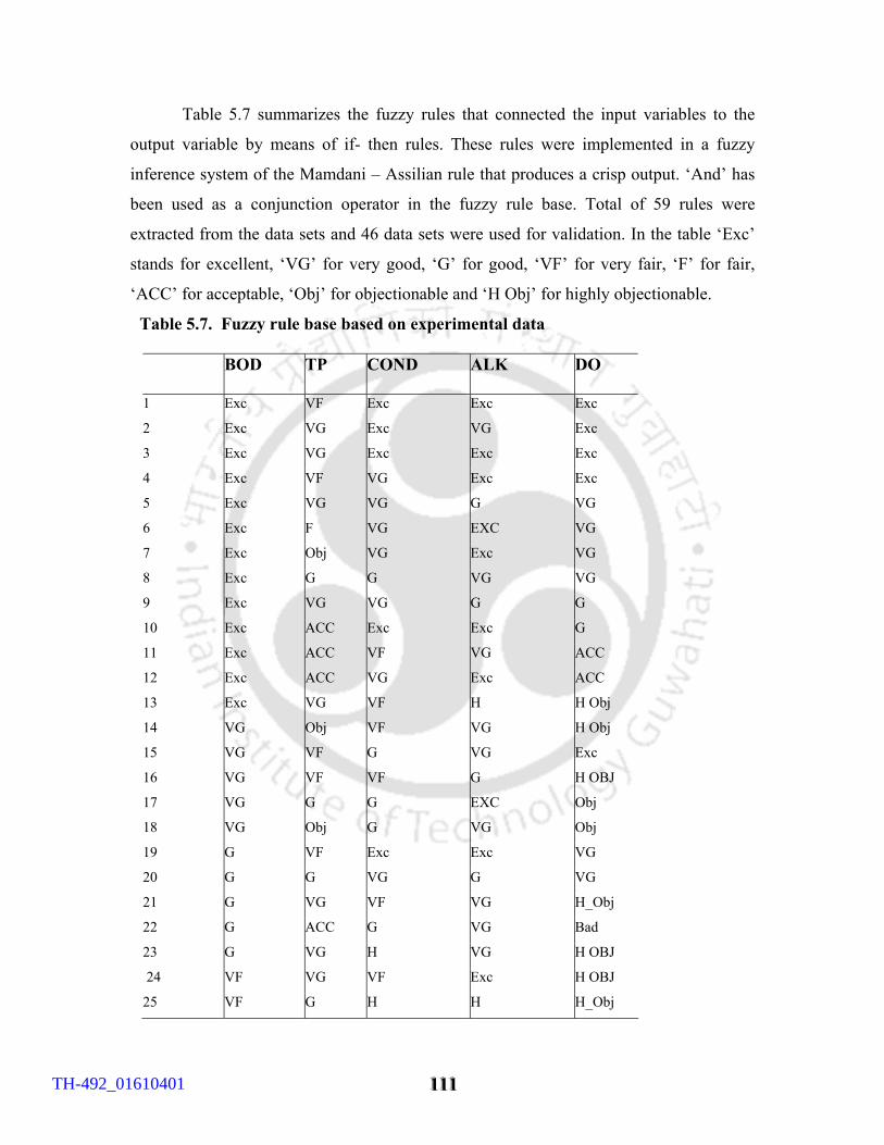
111111111

Table 5.7 summarizes the fuzzy rules that connected the input variables to the

output variable by means of if- then rules. These rules were implemented in a fuzzy

inference system of the Mamdani – Assilian rule that produces a crisp output. ‘And’ has

been used as a conjunction operator in the fuzzy rule base. Total of 59 rules were

extracted from the data sets and 46 data sets were used for validation. In the table ‘Exc’

stands for excellent, ‘VG’ for very good, ‘G’ for good, ‘VF’ for very fair, ‘F’ for fair,

‘ACC’ for acceptable, ‘Obj’ for objectionable and ‘H Obj’ for highly objectionable.

Table 5.7. Fuzzy rule base based on experimental data

BOD TP COND ALK DO

1 Exc VF Exc Exc Exc

2 Exc VG Exc VG Exc

3 Exc VG Exc Exc Exc

4 Exc VF VG Exc Exc

5 Exc VG VG G VG

6 Exc F VG EXC VG

7 Exc Obj VG Exc VG

8 Exc G G VG VG

9 Exc VG VG G G

10 Exc ACC Exc Exc G

11 Exc ACC VF VG ACC

12 Exc ACC VG Exc ACC

13 Exc VG VF H H Obj

14 VG Obj VF VG H Obj

15 VG VF G VG Exc

16 VG VF VF G H OBJ

17 VG G G EXC Obj

18 VG Obj G VG Obj

19 G VF Exc Exc VG

20 G G VG G VG

21 G VG VF VG H_Obj

22 G ACC G VG Bad

23 G VG H VG H OBJ

24 VF VG VF Exc H OBJ

25 VF G H H H_Obj

TH-492_01610401

111111222

26 F VG VG EXC EXC

27 F G VF H H_Obj

28 F Obj G VG H_Obj

29 F VF Vf VG H OBJ

30 F OBJ H G H_Obj

31 F Obj VF G H_Obj

32 F Obj VF G H_Obj

33 ACC VF G VG VG

34 ACC VF VG VG Obj

35 ACC F H VH H_Obj

36 ACC VF VF F H OBJ

37 ACC Obj VF VG H OBJ

38 ACC Obj G VG H OBJ

39 ACC G H F H_Obj

40 ACC F Exc EXC Bad

41 Obj Obj G G H_OBJ

42 Obj Obj H G H_OBJ

43 Obj Obj VF G H_OBJ

44 Obj F VF G H OBJ

45 Obj Obj VH H H_Obj


47 Obj Obj H F H_Obj


49 Obj ACC G VG H_OBJ

50 Obj Obj VF F H_OBJ


52 Obj Acc VF VG H_OBJ

53 Obj VF H G H_Obj

54 Obj Obj H G H_ OBJ

55 Obj VF H F H_OBJ

56 Obj VF VF Exc Obj

57 Obj G H H Obj

58 Obj Obj VH F H_Obj

59 Obj Obj VH G H_Obj

TH-492_01610401

111111333

After defining the linguistic variables and rules, next step is the determination of the

degree of membership of the input in the rule antecedents. In this model minimum –

operator is employed for the implication ‘and’,

the degree of match of the rule ‘r’ is

αr = mini=1……,n { inputi

jii x(µ ) }

here ‘i’ indicates the linguistic variable, I = 1,……..n; ‘j’ indicates the term of the

linguistic variable ‘i’, j = 1,……….,m(i), and m(i) is the number of terms of the

linguistic variable i. The results of the evaluation process is obtained by aggregation of

all consequences using the maximum operator which is given by:

µconseq (u) === max r { µ conseqr (u) }

where µ conseqr (u) = min { αr , µ

j (u)}

5.2.2 DEFUZZIFICATION

Defuzzification or decoding the outputs is the operation that produces a

nonfuzzy control action, a single crisp value ‘u’ that adequately represents the

membership function µconseq (u) of an aggregated fuzzy control action. The three often-

used methods are center of area (COA), which is also called center of gravity (COG),

center of sums (COS) and means of maxima (MOM) (Zimmermann 1996). Center of area

method is the most widely used method of the defuzzification method and consists of

selecting the value corresponding to the center of gravity of the solution set.

∫

∫=

u

conseq

conseq

u

duu

duuuu

)(

)(.

µ

µ

5.2.3 PERFORMANCE OF THE MODEL

In order to conduct quantitative comparison both the training datasets as

well as the validation data sets were fed in to the model and the defuzzified crisp values

were plotted with observations. RMSE (Root mean square error value), R2 (coefficient of

determination) value and E (Nash coefficient of efficiency) were used to evaluate the

model performance. RMSE is given by,

TH-492_01610401

111111444

RMSE = ∑ −n

mii xx

n 1

2 ))((1,

Where ix is the observed value of the ith data set and

mix is the respective model output.

The ideal value for RMSE is 0. Coefficient of determination is a statistical measure of

how well the regression line approximates the real data points. An R2 of 1 indicates that

the regression line perfectly fits the data. When the RMSE is minimum and R2 is high (>

0.8), a model can be judged as very good (Strik et.al, 2005). Nash efficiency is given by

the expression,

E = 1- ∑

∑

=

=

−

−

n

i

i

n

i

im

i

xx

xx

1

200

1

20

)(

)(

Where xo is the observed value , xm is the modeled value ,xi is the output of the ith data

set, 0x is the mean of the observations.The closer the model efficiency is to 1, the more

accurate the model is (Nash and Sutcliffe ,1970).

5.3 ARTIFICIAL NEURAL NETWORK MODEL

In this study, a three- layer feed forward artificial neural network (ANN) model

having four input neurons, one output neuron and seven hidden neurons was used as

shown in Figure 4.8. Dissolved oxygen concentration in water bodies is influenced by a

number of physical, chemical and biological factors. An attempt has been made to obtain

a relationship connecting biochemical oxygen demand, total phosphorus, conductivity

and alkalinity with dissolved oxygen concentration. 5.3.1 DATA NORMALIZATION

The input and output quantities were first normalized to a range of 0.1 to

0.9 with the following equations ::: nPi= 0.1+ 0.8 *(Pi – Pmin i)/(Pmax i - Pmin i )

nt = 0.1+ 0.8 *(ti – tmin i)/(tmax - tmin )

TH-492_01610401

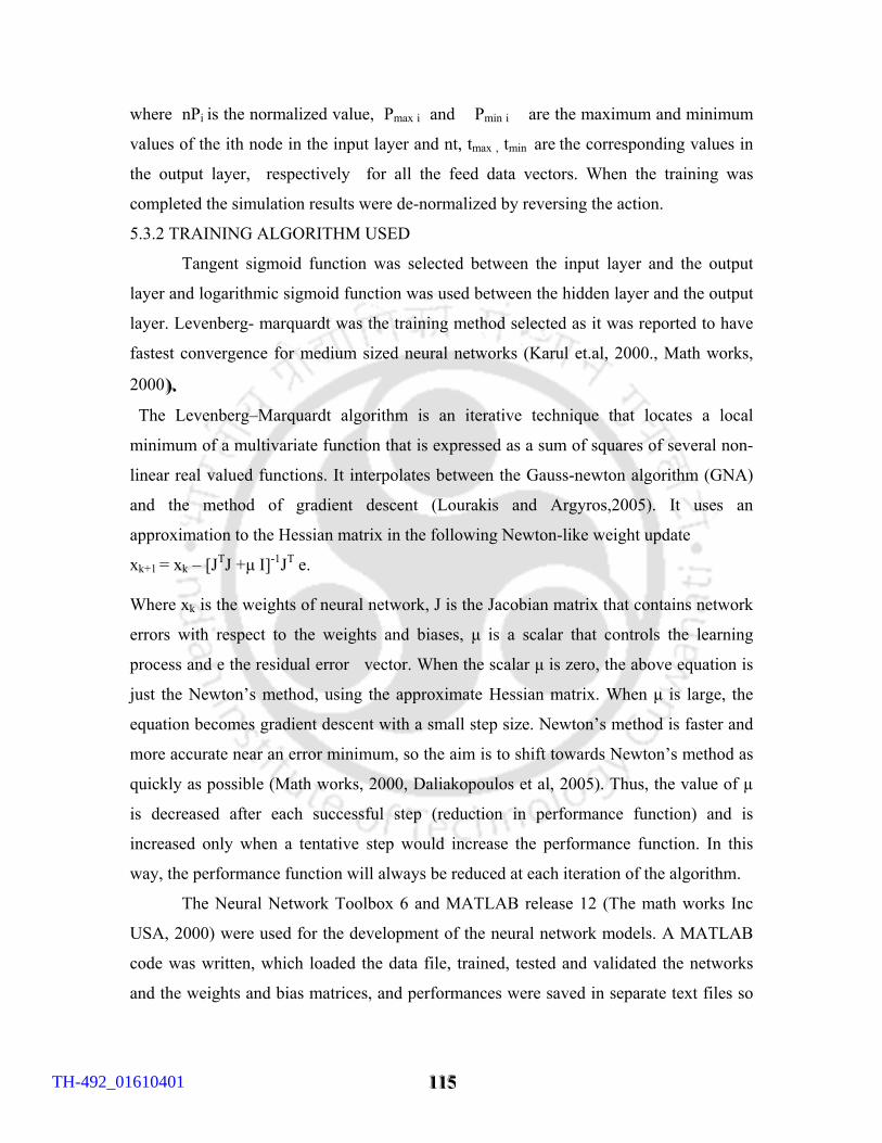
111111555

where nPi is the normalized value, Pmax i and Pmin i are the maximum and minimum

values of the ith node in the input layer and nt, tmax , tmin are the corresponding values in

the output layer, respectively for all the feed data vectors. When the training was

completed the simulation results were de-normalized by reversing the action. 5.3.2 TRAINING ALGORITHM USED

Tangent sigmoid function was selected between the input layer and the output

layer and logarithmic sigmoid function was used between the hidden layer and the output

layer. Levenberg- marquardt was the training method selected as it was reported to have

fastest convergence for medium sized neural networks (Karul et.al, 2000., Math works,

2000 )))... The Levenberg–Marquardt algorithm is an iterative technique that locates a local

minimum of a multivariate function that is expressed as a sum of squares of several non-

linear real valued functions. It interpolates between the Gauss-newton algorithm (GNA)

and the method of gradient descent (Lourakis and Argyros,2005). It uses an

approximation to the Hessian matrix in the following Newton-like weight update

xk+1 = xk – [JTJ +µ I]-1JT e.

Where xk is the weights of neural network, J is the Jacobian matrix that contains network

errors with respect to the weights and biases, µ is a scalar that controls the learning

process and e the residual error vector. When the scalar µ is zero, the above equation is

just the Newton’s method, using the approximate Hessian matrix. When µ is large, the

equation becomes gradient descent with a small step size. Newton’s method is faster and

more accurate near an error minimum, so the aim is to shift towards Newton’s method as

quickly as possible (Math works, 2000, Daliakopoulos et al, 2005). Thus, the value of µ

is decreased after each successful step (reduction in performance function) and is

increased only when a tentative step would increase the performance function. In this

way, the performance function will always be reduced at each iteration of the algorithm.

The Neural Network Toolbox 6 and MATLAB release 12 (The math works Inc

USA, 2000) were used for the development of the neural network models. A MATLAB

code was written, which loaded the data file, trained, tested and validated the networks

and the weights and bias matrices, and performances were saved in separate text files so

TH-492_01610401

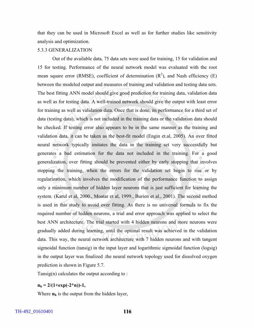
111111666

that they can be used in Microsoft Excel as well as for further studies like sensitivity

analysis and optimization.

5.3.3 GENERALIZATION

Out of the available data, 75 data sets were used for training, 15 for validation and

15 for testing. Performance of the neural network model was evaluated with the root

mean square error (RMSE), coefficient of determination (R2), and Nash efficiency (E)

between the modeled output and measures of training and validation and testing data sets. The best fitting ANN model should give good prediction for training data, validation data

as well as for testing data. A well-trained network should give the output with least error

for training as well as validation data. Once that is done, its performance for a third set of

data (testing data), which is not included in the training data or the validation data should

be checked. If testing error also appears to be in the same manner as the training and

validation data, it can be taken as the best-fit model (Engin et.al, 2005). An over fitted

neural network typically imitates the data in the training set very successfully but

generates a bad estimation for the data not included in the training. For a good

generalization, over fitting should be prevented either by early stopping that involves

stopping the training, when the errors for the validation set begin to rise or by

regularization, which involves the modification of the performance function to assign

only a minimum number of hidden layer neurons that is just sufficient for learning the

system. (Karul et al, 2000., Moatar et al, 1999., Burien et al., 2001). The second method

is used in this study to avoid over fitting. As there is no universal formula to fix the

required number of hidden neurons, a trial and error approach was applied to select the

best ANN architecture. The trial started with 4 hidden neurons and more neurons were

gradually added during learning, until the optimal result was achieved in the validation

data. This way, the neural network architecture with 7 hidden neurons and with tangent

sigmoidal function (tansig) in the input layer and logarithmic sigmoidal function (logsig)

in the output layer was finalized .the neural network topology used for dissolved oxygen

prediction is shown in Figure 5.7. Tansig(n) calculates the output according to :

nh = 2/(1+exp(-2*n))-1,

Where nh is the output from the hidden layer,

TH-492_01610401

111111777

and n = W1*P + b1

where W1 is the weight matrix connecting input and the hidden layer,

P is the input matrix

b1 is the bias .

Final output can be expressed in the form:

tm = logsig (W2*nh+b2) = 1/(1+exp(-(W2*(2/(1+exp(-2* (W1*P + b1 )))-1)+b2)),

Where

W2 and b2 are the weight and bias matrices connecting the hidden layer and the output

layer.

Figure 5.7 Neural network topology used in the study

Input layer Hidden layer Output layer

BOD

TP

CONDUCTIVITY

ALKALINITY

DO

TH-492_01610401

111111888

5.4 MULTIPLE LINEAR REGRESSION MODEL

The empirical relation is derived on the basis of obtained experimental results for

predicting dissolved oxygen in terms of BOD, TP, conductivity and alkalinity. Assuming

the variables agrees with the linear model,

Y=Xβ, where

Y is the n-by-1 matrix of output parameter,

X is the n-by-p matrix of input parameter,

β is the p-by-1 matrix of coefficients

β and ε are evaluated and the output variable was calculated by resubstituting the values.

In the first trial the relationship tried was

t n = K1 +K2 *p1n +K3*p2n+K4*p3n+K5*p4 n (4)

where tn is the output for the nth data set,

P1n , P2n , P3n & P4n are the input variable for the nth data set ,

K2 , K3 , K4 & K5 are the regression coefficients and

K1 is the constant where the regression line intercepts the y axis representing the

amount the dependant tn will be when all the independent variables are zero.

It can be represented in the matrix form as

Y=Xβ

tr1 1 p11 p21 p31 p41 K1

tr2 1 p12 p22 p32 p42 K2

Y= . X= . . . . . β= K3

. . . . . . K4

trn 1 p1n p2n p3n p4n K5

X is known as the sensitivity matrix. Using the least square method β can be

estimated as

β =(XTX)-1 XTY=V XTY.

TH-492_01610401

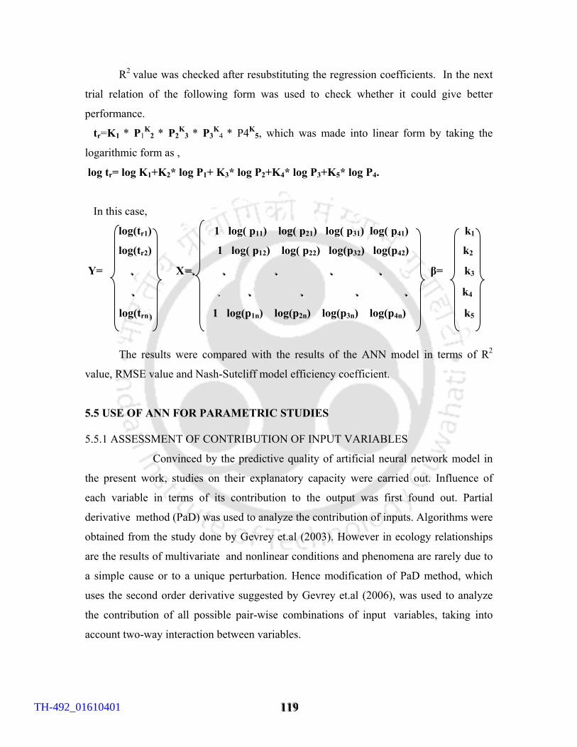
111111999

R2 value was checked after resubstituting the regression coefficients. In the next

trial relation of the following form was used to check whether it could give better

performance.

tr=K1 * P1K

2 * P2K

3 * P3K

4 * P4K5, which was made into linear form by taking the

logarithmic form as ,

log tr= log K1+K2* log P1+ K3* log P2+K4* log P3+K5* log P4.

In this case,

log(tr1) 1 log( p11) log( p21) log( p31) log( p41) k1

log(tr2) 1 log( p12) log( p22) log(p32) log(p42) k2

Y= ... X ===... ... ... ... ... β= k3

... ... ... ... ... ... k4

log(trn ))) 1 log(p1n) log(p2n) log(p3n) log(p4n) k5

The results were compared with the results of the ANN model in terms of R2

value, RMSE value and Nash-Sutcliff model efficiency coefficient.

5.5 USE OF ANN FOR PARAMETRIC STUDIES

5.5.1 ASSESSMENT OF CONTRIBUTION OF INPUT VARIABLES

Convinced by the predictive quality of artificial neural network model in

the present work, studies on their explanatory capacity were carried out. Influence of

each variable in terms of its contribution to the output was first found out. Partial

derivative method (PaD) was used to analyze the contribution of inputs. Algorithms were

obtained from the study done by Gevrey et.al (2003). However in ecology relationships

are the results of multivariate and nonlinear conditions and phenomena are rarely due to

a simple cause or to a unique perturbation. Hence modification of PaD method, which

uses the second order derivative suggested by Gevrey et.al (2006), was used to analyze

the contribution of all possible pair-wise combinations of input variables, taking into

account two-way interaction between variables.

TH-492_01610401

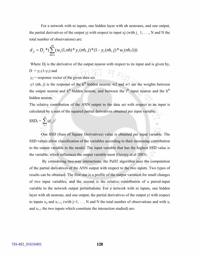
111222000

For a network with ni inputs, one hidden layer with nh neurones, and one output,

the partial derivatives of the output yj with respect to input xj (with j_/1, . . ., N and N the

total number of observations) are:

))),(*),(1(*),(*),1(((*1

1112∑=

−=nh

nhjji inhwjnhyjnhynhwDd

Where Dj is the derivative of the output neuron with respect to its input and is given by,

D = y2 (1-y2) and

y2 = response vector of the given data set.

y1 (nh, j) is the response of the hth hidden neuron, w2 and w1 are the weights between

the output neuron and hth hidden neuron, and between the ith input neuron and the hth

hidden neuron.

The relative contribution of the ANN output to the data set with respect to an input is

calculated by a sum of the squared partial derivatives obtained per input variable:

SSDi = 2

1)( ji

N

jd∑

=

One SSD (Sum of Square Derivatives) value is obtained per input variable. The

SSD values allow classification of the variables according to their increasing contribution

to the output variable in the model. The input variable that has the highest SSD value is

the variable, which influences the output variable most (Gevrey et.al 2003).

By considering two-way interactions, the PaD2 algorithm uses the computation

of the partial derivatives of the ANN output with respect to the two inputs. Two types of

results can be obtained. The first one is a profile of the output variation for small changes

of two input variables, and the second is the relative contribution of a paired-input

variable to the network output perturbations. For a network with ni inputs, one hidden

layer with nh neurons, and one output, the partial derivatives of the output yi with respect

to inputs xij and xi+1 j (with j=1, . . . N and N the total number of observations and with xi

and xi+1 the two inputs which constitute the interaction studied) are:

TH-492_01610401

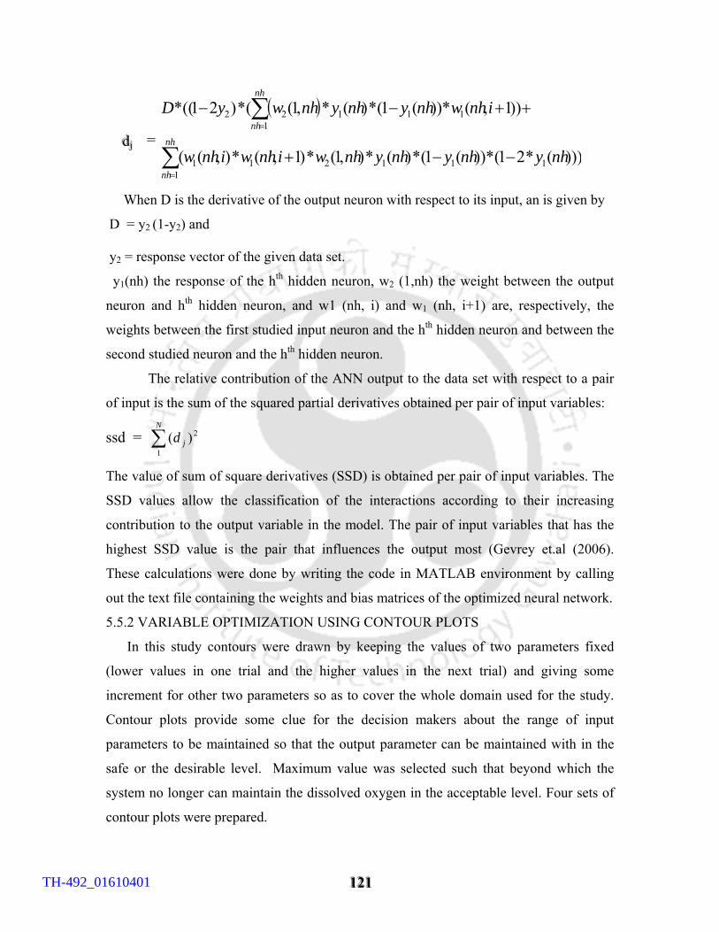
111222111

dddjjj =

( )

)))(*21(*))(1(*)(*),1(*)1,(*),((

))1,(*))(1(*)(*,1((*)21((*

111211

1

1111

22

nhynhynhynhwinhwinhw

inhwnhynhynhwyD

nh

nh

nh

nh

−−+

++−−

∑

∑

=

=

When D is the derivative of the output neuron with respect to its input, an is given by

D = y2 (1-y2) and

y2 = response vector of the given data set.

y1(nh) the response of the hth hidden neuron, w2 (1,nh) the weight between the output

neuron and hth hidden neuron, and w1 (nh, i) and w1 (nh, i+1) are, respectively, the

weights between the first studied input neuron and the hth hidden neuron and between the

second studied neuron and the hth hidden neuron.

The relative contribution of the ANN output to the data set with respect to a pair

of input is the sum of the squared partial derivatives obtained per pair of input variables:

ssd = 2

1)(∑

N

jd

The value of sum of square derivatives (SSD) is obtained per pair of input variables. The

SSD values allow the classification of the interactions according to their increasing

contribution to the output variable in the model. The pair of input variables that has the

highest SSD value is the pair that influences the output most (Gevrey et.al (2006).

These calculations were done by writing the code in MATLAB environment by calling

out the text file containing the weights and bias matrices of the optimized neural network.

5.5.2 VARIABLE OPTIMIZATION USING CONTOUR PLOTS

In this study contours were drawn by keeping the values of two parameters fixed

(lower values in one trial and the higher values in the next trial) and giving some

increment for other two parameters so as to cover the whole domain used for the study.

Contour plots provide some clue for the decision makers about the range of input

parameters to be maintained so that the output parameter can be maintained with in the

safe or the desirable level. Maximum value was selected such that beyond which the

system no longer can maintain the dissolved oxygen in the acceptable level. Four sets of

contour plots were prepared.

TH-492_01610401

111222222

1. Contour plots for DO concentrations vs TP and BOD, when

(a) Conductivity = 50 µS/cm and alkalinity = 25 mg/L,

(b) Conductivity = 300 µS /L and alkalinity =150 mg/L

2. Contour plots for DO concentration vs conductivity and alkalinity when

(a) BOD = 0 mg/L, TP = 0.03 mg/L (b) BOD =10 mg/L, TP= 1 mg/L.

3. Contour plots of DO concentration vs conductivity and BOD when

(a) alkalinity = 25 mg/L, TP = 0.04 mg/L. (b) alkalinity = 180 mg/L. TP = 1 mg/L.

4. Contour plots of DO concentration Vs conductivity and TP when

(a) BOD = 0 mg/L, alkalinity = 25 mg/L, (b). BOD = 8 mg/L, alkalinity = 200 mg/L.

After obtaining the contour plots for some specific values, original data sets with

output values above the desirable level were selected to obtain contour plots. This was

done to have a comparison and to check the reliability of the contour plots in parametric

studies.

5.6 SUMMARY

Based on the correlation coefficient the variables that were strongly correlated

with dissolved oxygen could be identified and those variables were selected as the input

variables for developing models. Three data driven models namely the fuzzy rule based

model, the artificial neural network model and the multiple linear regression model were

developed. Tuning of fuzzy rule based model was carried out by adding more fuzzy sets

and adding more rules to cover the entire pattern of the generated data sets. The ANN

model was tuned by optimizing the number of neurons in the hidden layer and then

assigning different transfer functions for the input layer and the output layer. The best-fit

model was arrived at by comparing the RMSE and R2 values obtained in each trial and

selecting that which produced the least RMSE. The purpose of developing multiple linear

regression models was to have a comparison with the artificial neural network. Nash

efficiency coefficient was also found to assess the predictive power of the model. Parametric studies were carried out to identify the most influencing parameter and to find

out the optimum range of each parameter to maintain the safe level of dissolved oxygen.

TH-492_01610401

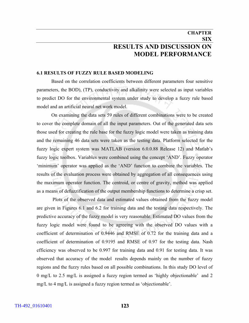
111222333

CHAPTER SIX RESULTS AND DISCUSSION ON MODEL PERFORMANCE

6.1 RESULTS OF FUZZY RULE BASED MODELING

Based on the correlation coefficients between different parameters four sensitive

parameters, the BOD), (TP), conductivity and alkalinity were selected as input variables

to predict DO for the environmental system under study to develop a fuzzy rule based

model and an artificial neural net work model.

On examining the data sets 59 rules of different combinations were to be created

to cover the complete domain of all the input parameters. Out of the generated data sets

those used for creating the rule base for the fuzzy logic model were taken as training data

and the remaining 46 data sets were taken as the testing data. Platform selected for the

fuzzy logic expert system was MATLAB (version 6.0.0.88 Release 12) and Matlab’s

fuzzy logic toolbox. Variables were combined using the concept ‘AND’. Fuzzy operator

‘minimum’ operator was applied as the ‘AND’ function to combine the variables. The

results of the evaluation process were obtained by aggregation of all consequences using

the maximum operator function. The centroid, or centre of gravity, method was applied

as a means of defuzzification of the output membership functions to determine a crisp set.

Plots of the observed data and estimated values obtained from the fuzzy model

are given in Figures 6.1 and 6.2 for training data and the testing data respectively. The

predictive accuracy of the fuzzy model is very reasonable. Estimated DO values from the

fuzzy logic model were found to be agreeing with the observed DO values with a

coefficient of determination of 0.9446 and RMSE of 0.72 for the training data and a coefficient of determination of 0.9195 and RMSE of 0.97 for the testing data. Nash

efficiency was observed to be 0.997 for training data and 0.91 for testing data. It was

observed that accuracy of the model results depends mainly on the number of fuzzy

regions and the fuzzy rules based on all possible combinations. In this study DO level of

0 mg/L to 2.5 mg/L is assigned a fuzzy region termed as ‘highly objectionable’ and 2

mg/L to 4 mg/L is assigned a fuzzy region termed as ‘objectionable’.

TH-492_01610401

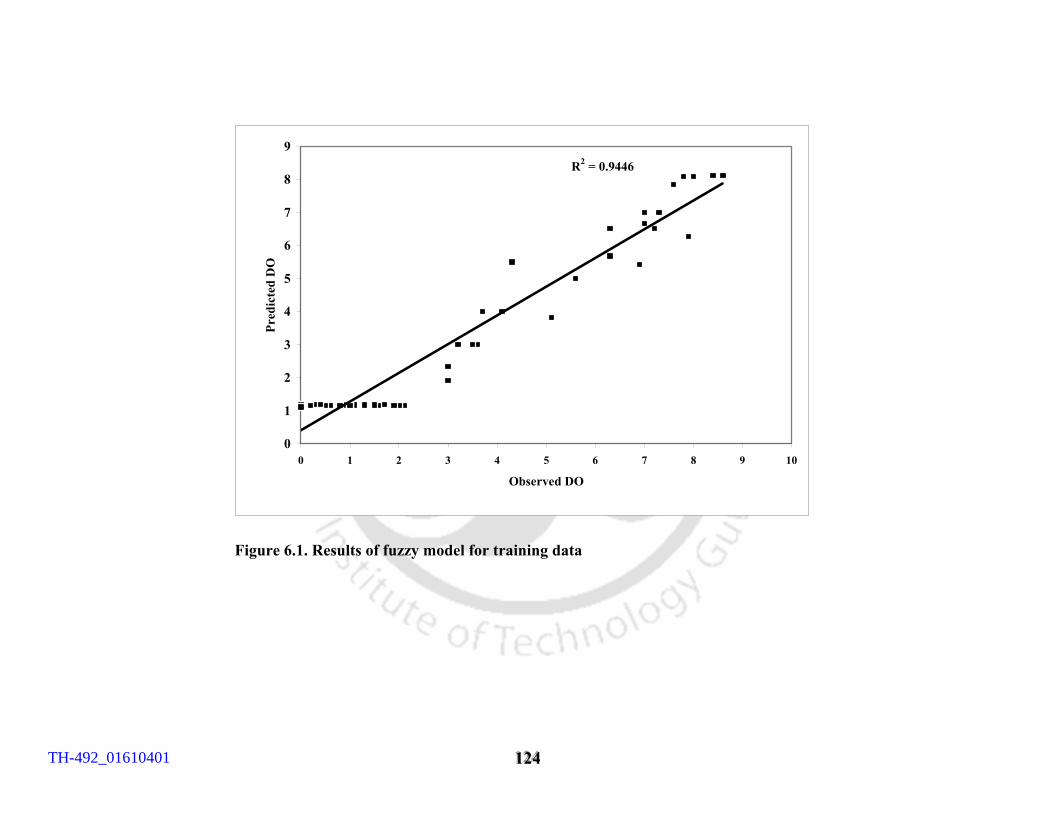
111222444

R2 = 0.9446

0

1

2

3

4

5

6

7

8

9

0 1 2 3 4 5 6 7 8 9 10

Observed DO

Pred

icte

d D

O

Figure 6.1. Results of fuzzy model for training data

TH-492_01610401

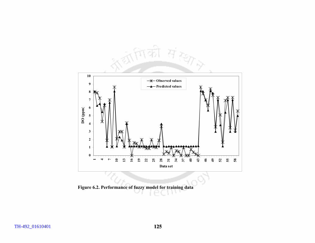
111222555

0

1

2

3

4

5

6

7

8

9

10

1 4 7 10 13 16 19 22 25 28 31 34 37 40 43 46 49 52 55 58

Data set

DO

(ppm

)Observed valuesPredicted values

Figure 6.2. Performance of fuzzy model for training data

TH-492_01610401

111222666

R2 = 0.9195

0

1

2

3

4

5

6

7

8

9

0 1 2 3 4 5 6 7 8 9

Observed DO

Pred

icte

d D

O

Figure 6.3 Results of fuzzy model for validation data.

TH-492_01610401

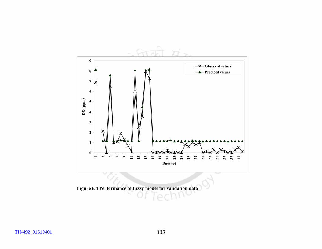
111222777

0

1

2

3

4

5

6

7

8

9

1 3 5 7 9 11 13 15 17 19 21 23 25 27 29 31 33 35 37 39 41

Data set

DO

(ppm

)

Observed valuesPrediced values

Figure 6.4 Performance of fuzzy model for validation data

TH-492_01610401

111222888

Results would have been more accurate if more number of fuzzy regions could be

included in between. But including fuzzy region for the DO levels below 4 mg/L was

considered meaningless in the practical sense as the whole region between 0 mg/L and 4

mg/L is considered highly objectionable.

While creating rule base and validating the model, it was observed that

fuzzy rule based models produce some unexpected failure. In particular, they are not able

to predict the output for an input data pattern, which is unknown to the model. This

concludes that the fuzzy rule based model is appropriate when it is possible introduce all

the possibilities in the rule base, as in the case of some mechanical or electronic tool. But

this is not the case with ecological modeling. When natural phenomena have to be dealt

with, the number of possible combinations may be large and the drawback observed in

this model will affect the prediction accuracy adversely.

6.1.1 CONCLUSIONS

Construction of a fuzzy rule based model is comparatively easy. The model is

data driven and can be trained further with every new set of data. The linguistic structure

of the model makes it transparent and easy to understand. The predictive accuracy of the

fuzzy model is quite reasonable. It was observed that accuracy of the model results

depends mainly on the number of fuzzy regions and the fuzzy rules based on all possible

combinations.

Though fuzzy rule based models produced satisfactory results some drawbacks

were observed while developing rule base. Accuracy of the results increases with

increase in membership functions with in the regions. This model is not able to execute a

forecast in some testing cases when the input vectors do not satisfy any “IF” condition of

the trained/calibrated rules. This concludes that the fuzzy rule based model is certainly

appropriate when it is possible introduce all the possibilities in the rule base, as in the

case of some mechanical or electronic tool, but it may not be totally reliable when dealing

with natural phenomenon where the number of possible combinations may be extremely

large as the model can not produce results for the input combinations that was not

considered in the training phase.

TH-492_01610401

111222999

6.2 ARTIFICIAL NEURAL NETWORK MODEL PERFORMANCE.

In this study a three- layer feed forward artificial neural network (ANN) model

having four input neurons, one output neuron and seven hidden neurons gave satisfactory

results. As the number of hidden neurons in the hidden layer can vary, and will affect the

quality of the ANN, an optimal number of hidden neurons were to be determined for the

neural network to achieve the best performance. As there is no universal formula to fix

the required number of hidden neurons, a trial and error approach was applied to select

the best ANN architecture. The trial started with 4 hidden neurons and gradually added

more during learning, until the optimal result was achieved in the validation data. Figure

5.23 shows the effect of hidden layer neurons on the performance of the ANN in the

study. This way the neural network architecture with 7 hidden neurons and with tangent

sigmoidal function in the input layer and logarithmic sigmoidal function in the out put

layer was finalized.

The RMS errors for the predicted results were 0.3222, 0.4994 and 0.5657 with

coefficients of determination of 0.9808, 0.9132 and 0.9563 and Nash efficiency

coefficient of 0.981, 0.970 and 0.962 for training data, testing data and validation data

respectively. Expression for output derived out from the ANN model is of the form,

tm = logsig (W2*nh+b2) = 1/(1+exp(-(W2*(2/(1+exp(-2* (W1*P + b1 )))-1)+b2)),

Where W1 is the weight matrix connecting input and the hidden layer,

P is the input matrix

b1 is the bias .

W2 and b2 are the weight and bias matrices connecting the hidden layer and the output

layer.

TH-492_01610401

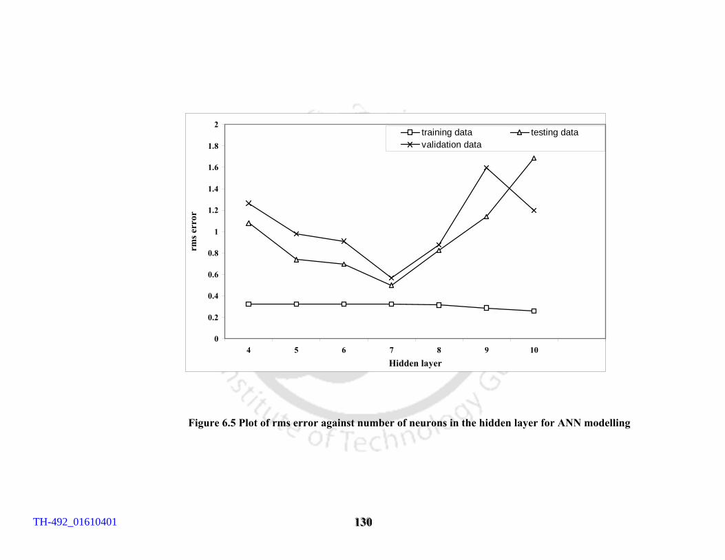
111333000

0

0.2

0.4

0.6

0.8

1

1.2

1.4

1.6

1.8

2

4 5 6 7 8 9 10Hidden layer

rms e

rror

training data testing datavalidation data

Figure 6.5 Plot of rms error against number of neurons in the hidden layer for ANN modelling

TH-492_01610401

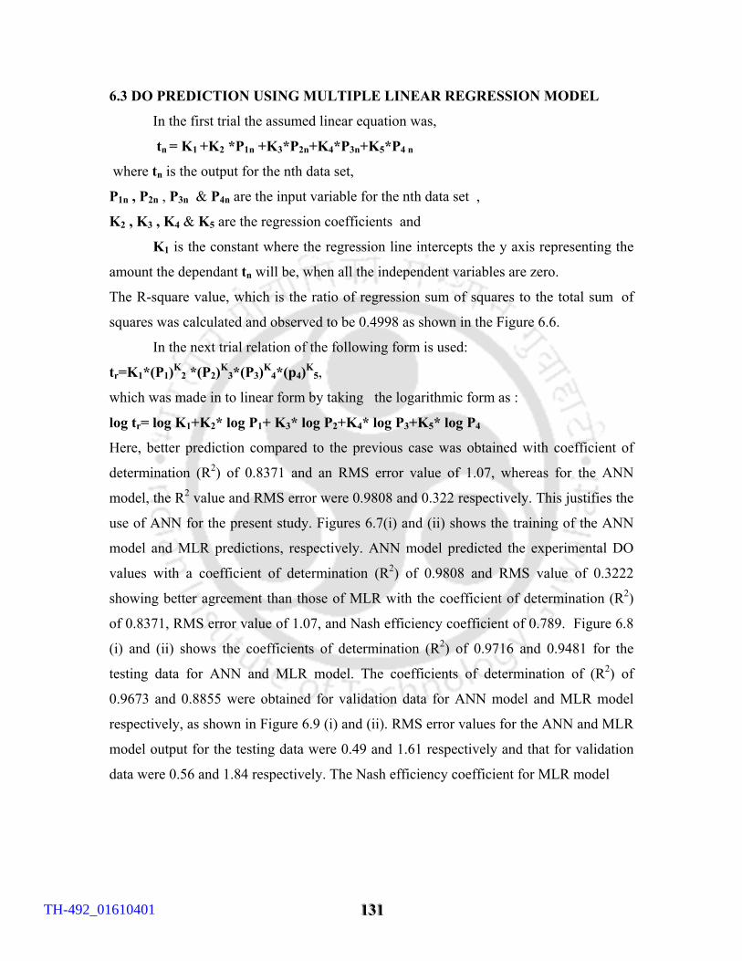
111333111

6.3 DO PREDICTION USING MULTIPLE LINEAR REGRESSION MODEL

In the first trial the assumed linear equation was,

tn = K1 +K2 *P1n +K3*P2n+K4*P3n+K5*P4 n

where tn is the output for the nth data set,

P1n , P2n , P3n & P4n are the input variable for the nth data set ,

K2 , K3 , K4 & K5 are the regression coefficients and

K1 is the constant where the regression line intercepts the y axis representing the

amount the dependant tn will be, when all the independent variables are zero.

The R-square value, which is the ratio of regression sum of squares to the total sum of

squares was calculated and observed to be 0.4998 as shown in the Figure 6.6.

In the next trial relation of the following form is used:

tr=K1*(P1)K2 *(P2)K

3*(P3)K4*(p4)K

5,

which was made in to linear form by taking the logarithmic form as :

log tr= log K1+K2* log P1+ K3* log P2+K4* log P3+K5* log P4

Here, better prediction compared to the previous case was obtained with coefficient of

determination (R2) of 0.8371 and an RMS error value of 1.07, whereas for the ANN

model, the R2 value and RMS error were 0.9808 and 0.322 respectively. This justifies the

use of ANN for the present study. Figures 6.7(i) and (ii) shows the training of the ANN

model and MLR predictions, respectively. ANN model predicted the experimental DO

values with a coefficient of determination (R2) of 0.9808 and RMS value of 0.3222

showing better agreement than those of MLR with the coefficient of determination (R2)

of 0.8371, RMS error value of 1.07, and Nash efficiency coefficient of 0.789. Figure 6.8

(i) and (ii) shows the coefficients of determination (R2) of 0.9716 and 0.9481 for the

testing data for ANN and MLR model. The coefficients of determination of (R2) of

0.9673 and 0.8855 were obtained for validation data for ANN model and MLR model respectively, as shown in Figure 6.9 (i) and (ii). RMS error values for the ANN and MLR

model output for the testing data were 0.49 and 1.61 respectively and that for validation

data were 0.56 and 1.84 respectively. The Nash efficiency coefficient for MLR model

TH-492_01610401

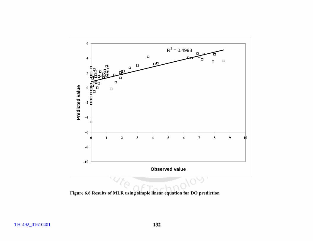
111333222

R2 = 0.4998

-10

-8

-6

-4

-2

0

2

4

6

0 1 2 3 4 5 6 7 8 9 10

Observed value

Pred

icte

d va

lue

Figure 6.6 Results of MLR using simple linear equation for DO prediction

TH-492_01610401

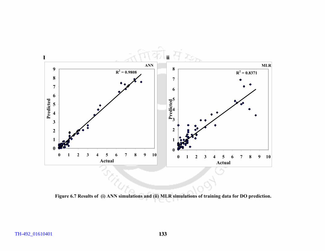
111333333

III ANN

R2 = 0.9808

0

1

2

3

4

5

6

7

8

9

0 1 2 3 4 5 6 7 8 9 10Actual

Pred

icte

d

iiiiii MLR

R2 = 0.8371

0

1

2

3

4

5

6

7

8

0 1 2 3 4 5 6 7 8 9 10Actual

Pred

icte

d

Figure 6.7 Results of (i) ANN simulations and (ii) MLR simulations of training data for DO prediction.

TH-492_01610401

111333444

iii...

R2 = 0.9716

0

1

2

3

4

5

6

7

8

9

10

0 1 2 3 4 5 6 7 8 9Observed

Pred

icte

d

iiiiii...

R2 = 0.9481

0

1

2

3

4

5

6

7

8

0 1 2 3 4 5 6 7 8 9Observed

Pred

icte

d

Figure 6.8 Results of (i) ANN simulations and (ii) MLR simulations of testing data for DO prediction.

TH-492_01610401

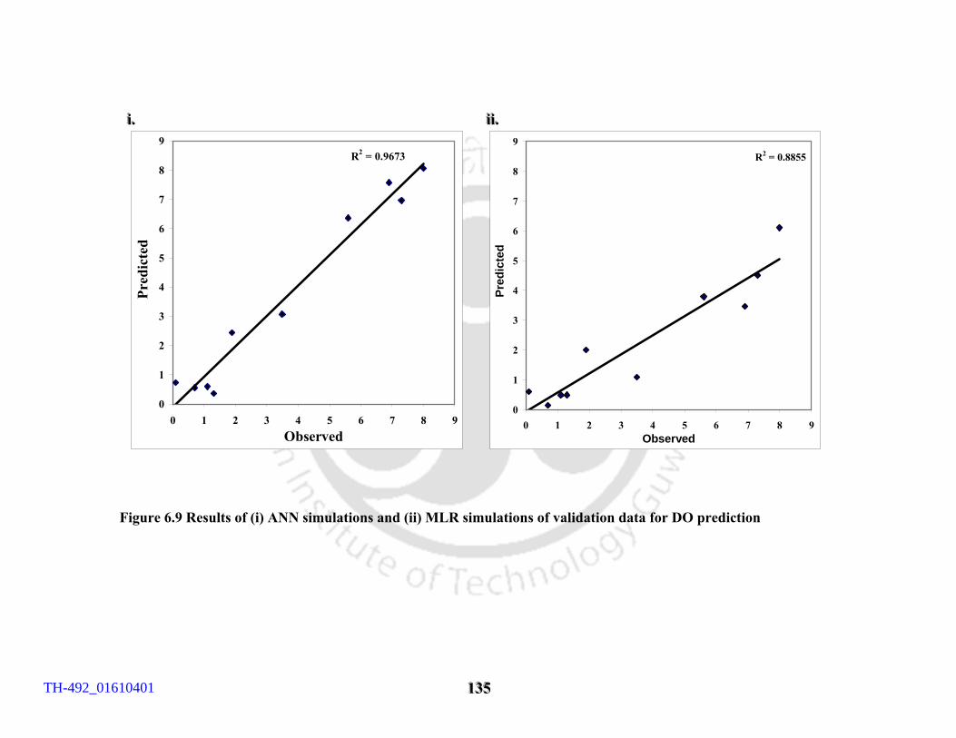
111333555

iii...

R2 = 0.9673

0

1

2

3

4

5

6

7

8

9

0 1 2 3 4 5 6 7 8 9Observed

Pred

icte

d

iiiiii...

R2 = 0.8855

0

1

2

3

4

5

6

7

8

9

0 1 2 3 4 5 6 7 8 9Observed

Pred

icte

d

Figure 6.9 Results of (i) ANN simulations and (ii) MLR simulations of validation data for DO prediction

TH-492_01610401

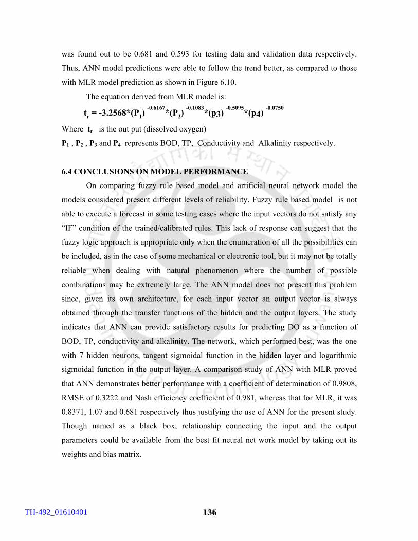
111333666

was found out to be 0.681 and 0.593 for testing data and validation data respectively.

Thus, ANN model predictions were able to follow the trend better, as compared to those

with MLR model prediction as shown in Figure 6.10.

The equation derived from MLR model is:

tr = -3.2568*(P1) -0.6167*(P2)

-0.1083*(p3) -0.5095*(p4) -0.0750

Where tr is the out put (dissolved oxygen)

P1 , P2 , P3 and P4 represents BOD, TP, Conductivity and Alkalinity respectively.

6.4 CONCLUSIONS ON MODEL PERFORMANCE

On comparing fuzzy rule based model and artificial neural network model the

models considered present different levels of reliability. Fuzzy rule based model is not

able to execute a forecast in some testing cases where the input vectors do not satisfy any

“IF” condition of the trained/calibrated rules. This lack of response can suggest that the

fuzzy logic approach is appropriate only when the enumeration of all the possibilities can

be included, as in the case of some mechanical or electronic tool, but it may not be totally

reliable when dealing with natural phenomenon where the number of possible

combinations may be extremely large. The ANN model does not present this problem

since, given its own architecture, for each input vector an output vector is always

obtained through the transfer functions of the hidden and the output layers. The study

indicates that ANN can provide satisfactory results for predicting DO as a function of

BOD, TP, conductivity and alkalinity. The network, which performed best, was the one

with 7 hidden neurons, tangent sigmoidal function in the hidden layer and logarithmic

sigmoidal function in the output layer. A comparison study of ANN with MLR proved

that ANN demonstrates better performance with a coefficient of determination of 0.9808,

RMSE of 0.3222 and Nash efficiency coefficient of 0.981, whereas that for MLR, it was

0.8371, 1.07 and 0.681 respectively thus justifying the use of ANN for the present study.

Though named as a black box, relationship connecting the input and the output

parameters could be available from the best fit neural net work model by taking out its

weights and bias matrix.

TH-492_01610401

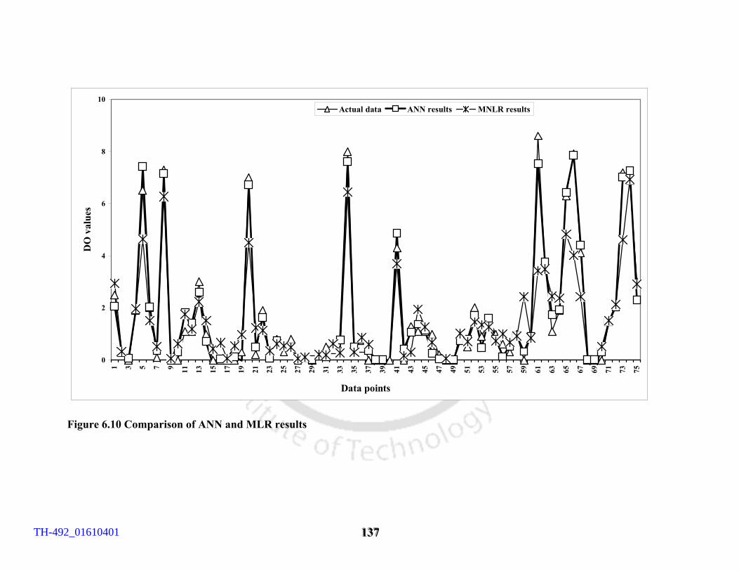
111333777

0

2

4

6

8

10

1 3 5 7 9 11 13 15 17 19 21 23 25 27 29 31 33 35 37 39 41 43 45 47 49 51 53 55 57 59 61 63 65 67 69 71 73 75

Data points

DO

val

ues

Actual data ANN results MNLR results

Figure 6.10 Comparison of ANN and MLR results

TH-492_01610401

111333888

6.5 CONRIBUTION OF VARIABLES USING SIMULATED NEURAL

NETWORK For assessing the contribution of each input variable partial derivative method

(PaD) suggested by Gevrey et al (2003) was adopted in the present study. By using

partial derivative method, two results could be obtained. One is the profile of the output

variation and second is the classification of relative contribution of each variable to the

network output.

Figure 6.11 presents the derivative plots of PaD method. Partial derivative values

of dissolved oxygen with respect to BOD were negative. This indicates that output

variable decreases with increase in BOD.When microorganisms begin the process of

breaking down the organic matter like dead plants, leaves manure, sewage and even food

waste present in the water body, much of the available dissolved oxygen is consumed by

aerobic bacteria, robbing other aquatic organisms of the oxygen they need to live. Hence

higher quantity of BOD indicates large quantity of organic matter and decrease in

dissolved oxygen in the water body, which is evident from the profile plot as well. Partial

derivative values of DO with respect to TP are all positive and near zero at higher values.

This means that dissolved oxygen increases with increase in TP but to a lesser extent for

higher values. Though the ultimate effect of excess level of nutrients is the depletion of

dissolved oxygen, this depletion is the result of algal crashes which ends up in high BOD

and which in turn results in DO depletion. Immediate effect of algal and other submerged

plant growth is the oxygen transfer into the water body during the day through

photosynthesis. Partial derivative of DO with respect to conductivity are positive and

negative without a precise direction. It may be due to its interaction with other variables.

However the values for lower concentrations are negative. Partial derivative values for

DO with respect to alkalinity are all positive which implies that an increase in alkalinity

will lead to an increase of dissolved oxygen but to a lesser extent for the higher values of

alkalinity. Partial derivative method showed that total phosphorus is the highest

contributed variable followed by conductivity, alkalinity and BOD (Figure 6.12).

TH-492_01610401

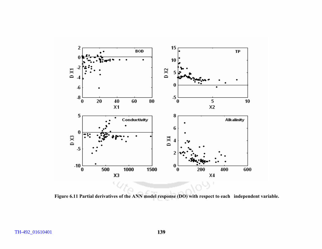
111333999

Figure 6.11 Partial derivatives of the ANN model response (DO) with respect to each independent variable.

TH-492_01610401

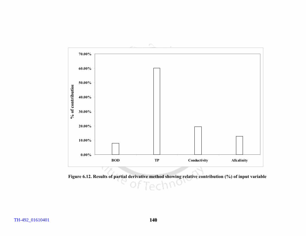
111444000

0.00%

10.00%

20.00%

30.00%

40.00%

50.00%

60.00%

70.00%

BOD TP Conductivity Alkalinity

% o

f con

trib

utio

n

Figure 6.12. Results of partial derivative method showing relative contribution (%) of input variable

TH-492_01610401

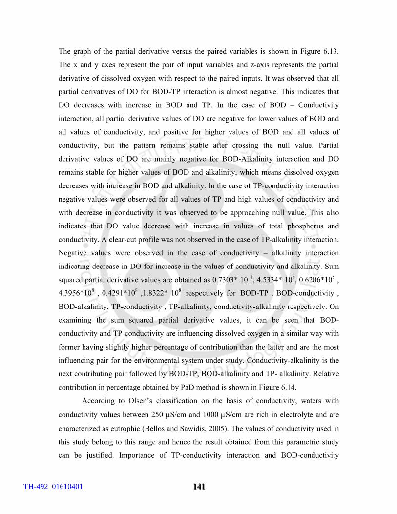
111444111

The graph of the partial derivative versus the paired variables is shown in Figure 6.13.

The x and y axes represent the pair of input variables and z-axis represents the partial

derivative of dissolved oxygen with respect to the paired inputs. It was observed that all

partial derivatives of DO for BOD-TP interaction is almost negative. This indicates that

DO decreases with increase in BOD and TP. In the case of BOD – Conductivity

interaction, all partial derivative values of DO are negative for lower values of BOD and

all values of conductivity, and positive for higher values of BOD and all values of

conductivity, but the pattern remains stable after crossing the null value. Partial

derivative values of DO are mainly negative for BOD-Alkalinity interaction and DO

remains stable for higher values of BOD and alkalinity, which means dissolved oxygen

decreases with increase in BOD and alkalinity. In the case of TP-conductivity interaction

negative values were observed for all values of TP and high values of conductivity and

with decrease in conductivity it was observed to be approaching null value. This also

indicates that DO value decrease with increase in values of total phosphorus and

conductivity. A clear-cut profile was not observed in the case of TP-alkalinity interaction.

Negative values were observed in the case of conductivity – alkalinity interaction

indicating decrease in DO for increase in the values of conductivity and alkalinity. Sum

squared partial derivative values are obtained as 0.7303* 10 8, 4.5334* 108, 0.6206*108 ,

4.3956*108 , 0.4291*108 ,1.8322* 108 respectively for BOD-TP , BOD-conductivity ,

BOD-alkalinity, TP-conductivity , TP-alkalinity, conductivity-alkalinity respectively. On

examining the sum squared partial derivative values, it can be seen that BOD-

conductivity and TP-conductivity are influencing dissolved oxygen in a similar way with

former having slightly higher percentage of contribution than the latter and are the most

influencing pair for the environmental system under study. Conductivity-alkalinity is the

next contributing pair followed by BOD-TP, BOD-alkalinity and TP- alkalinity. Relative

contribution in percentage obtained by PaD method is shown in Figure 6.14.

According to Olsen’s classification on the basis of conductivity, waters with

conductivity values between 250 µS/cm and 1000 µS/cm are rich in electrolyte and are

characterized as eutrophic (Bellos and Sawidis, 2005). The values of conductivity used in

this study belong to this range and hence the result obtained from this parametric study

can be justified. Importance of TP-conductivity interaction and BOD-conductivity

TH-492_01610401

111444222

Figure 6.13 Partial derivative of DO 3D graph for two-way interaction

X1-BOD, X2-TP, X3-Conductivity, X4-Total alkalinity.

TH-492_01610401

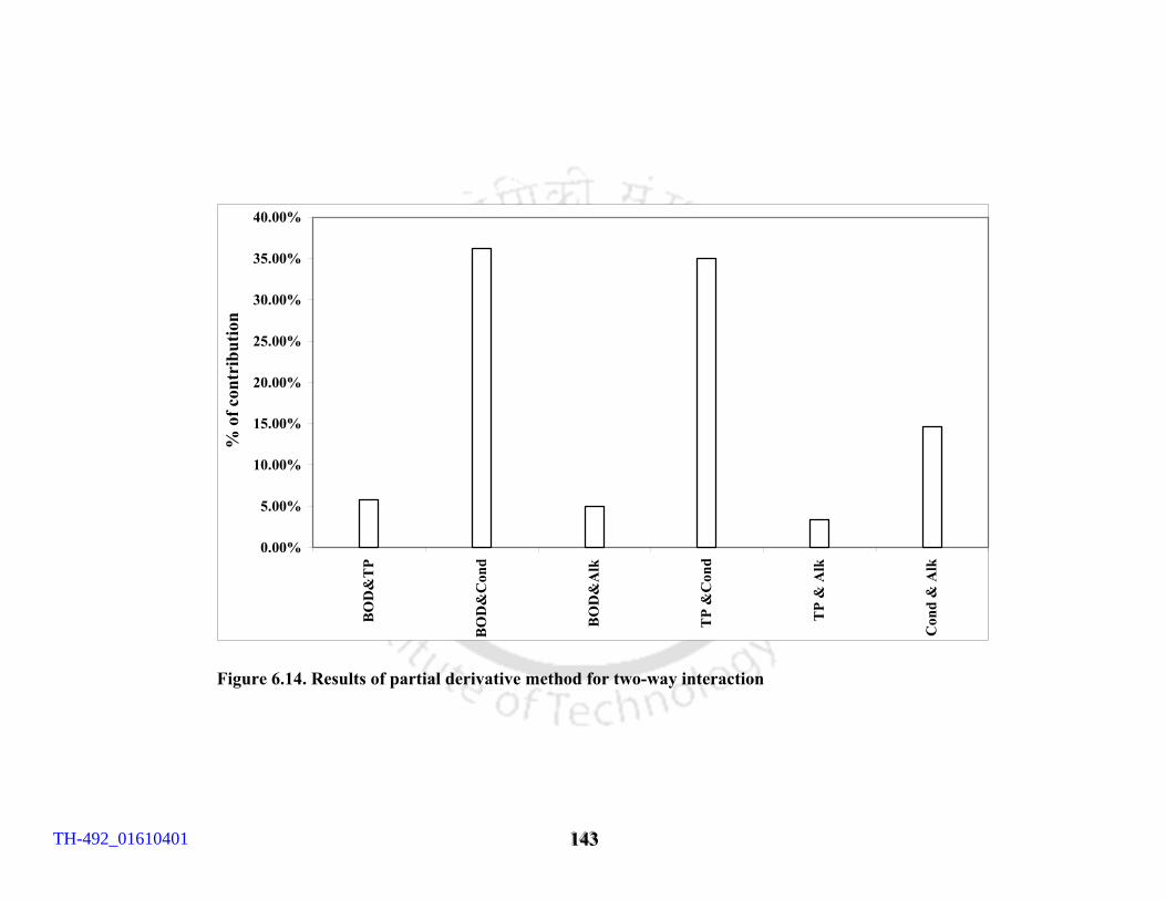
111444333

0.00%

5.00%

10.00%

15.00%

20.00%

25.00%

30.00%

35.00%

40.00%

BO

D&

TP

BO

D&

Con

d

BO

D&

Alk

TP

&C

ond

TP

& A

lk

Con

d &

Alk

% o

f con

trib

utio

n

Figure 6.14. Results of partial derivative method for two-way interaction

TH-492_01610401

111444444

interaction can hence be justified. Studies done by Gevrey et al (2003) and Olden et al

(2004) proved that partial derivative method seemed to be the reliable methodology for

assessing the contribution of input variables using simulated ANN model and this

tempted to adopt partial derivative method in the present study. Another advantage of

PaD method is that apart from obtaining the relative contribution of input variables,

profile of the output variations for small changes of the input variables could also be

obtained. It is possible to rank the inputs of the ANN one by one or by paired input

combination in order of contribution.

6.5.1 CONCLUSIONS

It is clear from this study that in ecology, using a single variable sensitivity

analysis may lead to misleading interpretation. In this study with single input sensitivity

analysis BOD seemed to be the least contributing variable, but is having a major role with

the interaction of conductivity. Hence it is evident that we must consider variable

interaction since environment is composed of many characteristics acting together.

Behaviour of the profile plots obtained from the two-way interaction also justifies the

values of the correlation coefficient, which concludes that selection of input variable

based on correlation coefficient is a reliable method. 6.6 OPTIMIZATION OF VARIABLES USING CONTOUR PLOTS

Figures 6.15, 6.16, 6.17, 6.18, 6.19, 6.20, 6.21 and 6.22 presents the contour plots

of dissolved oxygen concentration as a function of BOD, TP, conductivity and alkalinity.

These plots were drawn by simulating the best fit ANN model by assigning some values

for two parameters and giving some increments for the other two.

Figures 6.15 and 6.16 indicate that an optimal region exists in which the dissolved

oxygen concentrations can be maintained within the safe limits. BOD should be below 6

mg/L and TP should be below 1 mg/L, in order to maintain the DO above the desirable

level of 6 mg/L when conductivity and alkalinity are 50 µS/cm and 25 mg/L respectively

and TP values are low. BOD and TP should be below 11 mg/L and 1 mg/L respectively

to maintain the DO above the minimum tolerable level of 4 mg/L. For a conductivity of

300 µS/cm and an alkalinity of 150 mg/L, DO will be within the desirable level for a

BOD of 3 mg/L and TP of 0.4 mg/L. BOD should be below 8.5 mg/L and TP should be

below 1.2 mg/L to maintain a DO level above the maximum tolerable level of 4mg/L.

TH-492_01610401

111444555

Figures 6.17 and 6.18 indicate that an optimal region exists within which the

dissolved oxygen concentration can be maintained below the safe limits. Conductivity

should be below 275 µS/cm and alkalinity should be below 125 mg/L to maintain the DO

level above 4 mg/L. To maintain DO concentration above 6 mg/L, conductivity should

be below 225 µS/cm and alkalinity should be below 200 mg/L when BOD and TP values

are the least. For values of BOD =10 mg/L and TP = 1mg/L, dissolved oxygen cannot be

maintained above 6 mg/L. To maintain DO above 4 mg/L, conductivity should be below

150 µS/cm and alkalinity should be below 75 mg/L.

Figure 6.19 demonstrates that for least values of TP and alkalinity (0.04 mg/L and

25 mg/L respectively) DO can be maintained within the desirable limit by controlling the

conductivity below 200 µS/cm and BOD values below 4 mg/L. BOD values can go up to

12 mg/L for conductivity values ranging from 50 µS/cm to 100 µS/cm, whereas Figure

6.20 shows that conductivity values in the range of 750 µS/cm to 1500 µS/cm and BOD

values below 2 mg/L provides a safe domain of dissolved oxygen when alkalinity is

180 mg/L and total phosphorus of 1mg/L.This implies that for the range between 25

mg/L and 180 mg/L of alkalinity and total phosphorus between 0.04 mg/L to 1 mg/L,

with BOD below 6 mg/L dissolved oxygen will be above the desirable range of 5 mg/L

for conductivity values below 200 µS/cm and between 750 µS/cm and 900 µS/cm.

Figure 6.21 shows that conductivity below 250 µS/cm and TP below 2 mg/L is the safe

domain for DO for a value of BOD of 0 mg/L and alkalinity of 25 mg/L. However, BOD

should be below 8 mg/L and alkalinity should be below 200 mg/L, conductivity should

be between 225 µS/cm to 275 µS/cm and TP should be less than 0.2 mg/L for DO to be

above the desirable level of 6 mg/L as shown in Figure 6.22.

TH-492_01610401

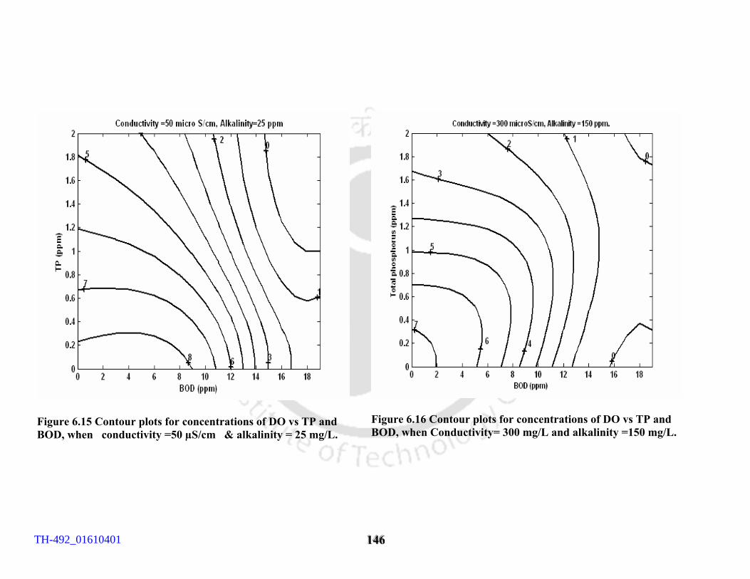
111444666

Figure 6.15 Contour plots for concentrations of DO vs TP and BOD, when conductivity =50 µS/cm & alkalinity = 25 mg/L.

Figure 6.16 Contour plots for concentrations of DO vs TP and BOD, when Conductivity= 300 mg/L and alkalinity =150 mg/L.

TH-492_01610401

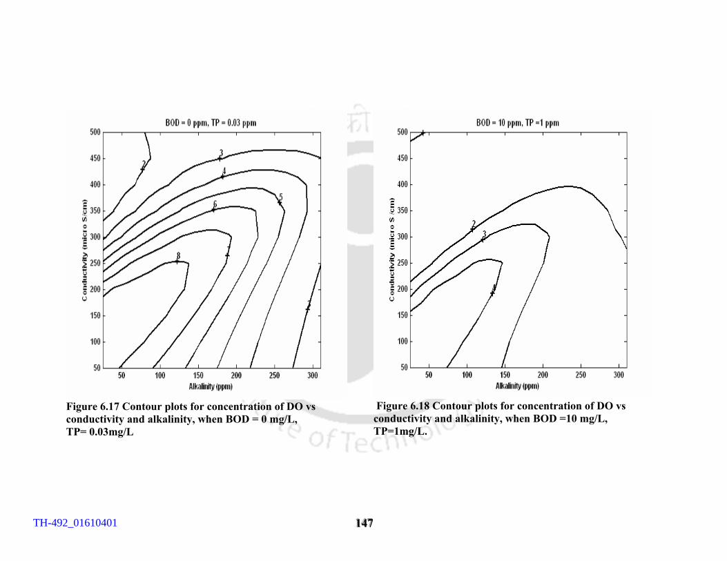
111444777

Figure 6.17 Contour plots for concentration of DO vs conductivity and alkalinity, when BOD = 0 mg/L, TP= 0.03mg/L

Figure 6.18 Contour plots for concentration of DO vs conductivity and alkalinity, when BOD =10 mg/L, TP=1mg/L.

TH-492_01610401

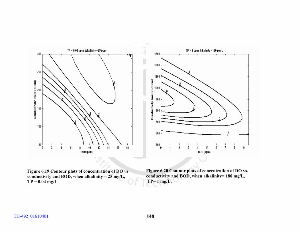
111444888

Figure 6.19 Contour plots of concentration of DO vs conductivity and BOD, when alkalinity = 25 mg/L, TP = 0.04 mg/L

Figure 6.20 Contour plots of concentration of DO vs. conductivity and BOD, when alkalinity= 180 mg/L, TP= 1 mg/L.

TH-492_01610401

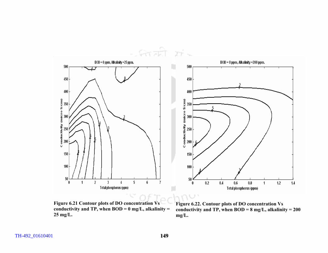
111444999

Figure 6.21 Contour plots of DO concentration Vs conductivity and TP, when BOD = 0 mg/L, alkalinity = 25 mg/L.

Figure 6.22. Contour plots of DO concentration Vs conductivity and TP, when BOD = 8 mg/L, alkalinity = 200 mg/L.

TH-492_01610401

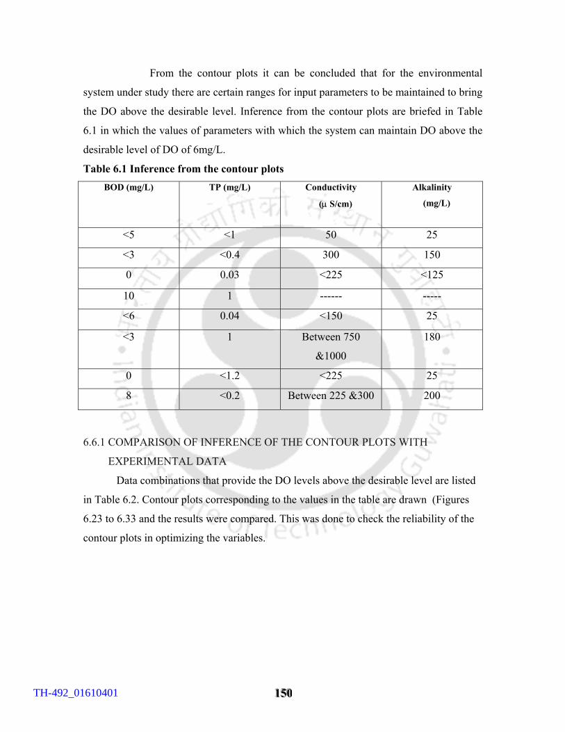
111555000

From the contour plots it can be concluded that for the environmental

system under study there are certain ranges for input parameters to be maintained to bring

the DO above the desirable level. Inference from the contour plots are briefed in Table

6.1 in which the values of parameters with which the system can maintain DO above the

desirable level of DO of 6mg/L.

Table 6.1 Inference from the contour plots BOD (mg/L) TP (mg/L) Conductivity

(µ S/cm)

Alkalinity

(mg/L)

<5 <1 50 25

<3 <0.4 300 150

0 0.03 <225 <125

10 1 ------ -----

<6 0.04 <150 25

<3 1 Between 750

&1000

180

0 <1.2 <225 25

8 <0.2 Between 225 &300 200

6.6.1 COMPARISON OF INFERENCE OF THE CONTOUR PLOTS WITH

EXPERIMENTAL DATA

Data combinations that provide the DO levels above the desirable level are listed

in Table 6.2. Contour plots corresponding to the values in the table are drawn (Figures

6.23 to 6.33 and the results were compared. This was done to check the reliability of the

contour plots in optimizing the variables.

TH-492_01610401

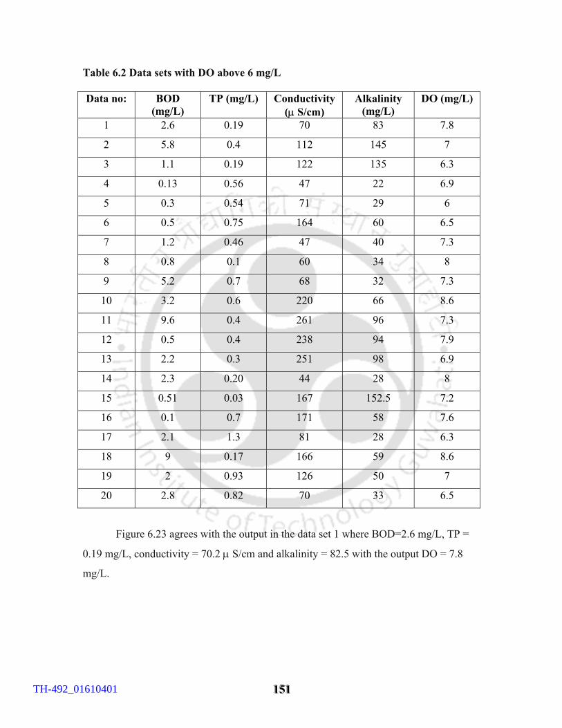
111555111

Table 6.2 Data sets with DO above 6 mg/L

Data no: BOD (mg/L)

TP (mg/L) Conductivity (µ S/cm)

Alkalinity (mg/L)

DO (mg/L)

1 2.6 0.19 70 83 7.8

2 5.8 0.4 112 145 7

3 1.1 0.19 122 135 6.3

4 0.13 0.56 47 22 6.9

5 0.3 0.54 71 29 6

6 0.5 0.75 164 60 6.5

7 1.2 0.46 47 40 7.3

8 0.8 0.1 60 34 8

9 5.2 0.7 68 32 7.3

10 3.2 0.6 220 66 8.6

11 9.6 0.4 261 96 7.3

12 0.5 0.4 238 94 7.9

13 2.2 0.3 251 98 6.9

14 2.3 0.20 44 28 8

15 0.51 0.03 167 152.5 7.2

16 0.1 0.7 171 58 7.6

17 2.1 1.3 81 28 6.3

18 9 0.17 166 59 8.6

19 2 0.93 126 50 7

20 2.8 0.82 70 33 6.5

Figure 6.23 agrees with the output in the data set 1 where BOD=2.6 mg/L, TP =

0.19 mg/L, conductivity = 70.2 µ S/cm and alkalinity = 82.5 with the output DO = 7.8

mg/L.

TH-492_01610401

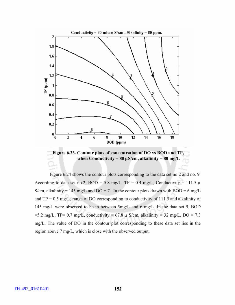
111555222

Figure 6.23. Contour plots of concentration of DO vs BOD and TP, when Conductivity = 80 µS/cm, alkalinity = 80 mg/L

Figure 6.24 shows the contour plots corresponding to the data set no 2 and no. 9.

According to data set no.2, BOD = 5.8 mg/L, TP = 0.4 mg/L, Conductivity = 111.5 µ

S/cm, alkalinity = 145 mg/L and DO = 7. In the contour plots drawn with BOD = 6 mg/L

and TP = 0.5 mg/L, range of DO corresponding to conductivity of 111.5 and alkalinity of

145 mg/L were observed to be in between 5mg/L and 6 mg/L. In the data set 9, BOD

=5.2 mg/L, TP= 0.7 mg/L, conductivity = 67.8 µ S/cm, alkalinity = 32 mg/L, DO = 7.3

mg/L. The value of DO in the contour plot corresponding to these data set lies in the

region above 7 mg/L, which is close with the observed output.

TH-492_01610401

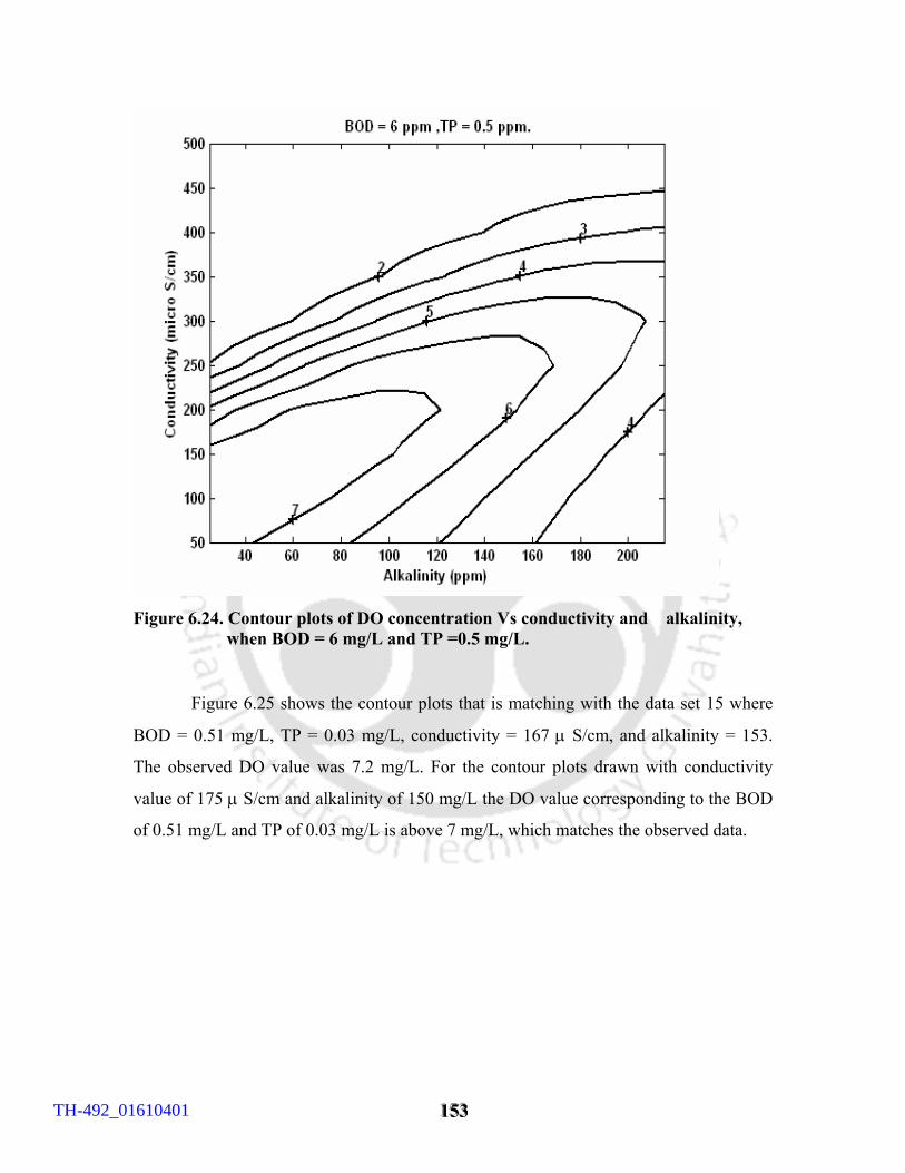
111555333

Figure 6.24. Contour plots of DO concentration Vs conductivity and alkalinity, when BOD = 6 mg/L and TP =0.5 mg/L.

Figure 6.25 shows the contour plots that is matching with the data set 15 where

BOD = 0.51 mg/L, TP = 0.03 mg/L, conductivity = 167 µ S/cm, and alkalinity = 153.

The observed DO value was 7.2 mg/L. For the contour plots drawn with conductivity

value of 175 µ S/cm and alkalinity of 150 mg/L the DO value corresponding to the BOD

of 0.51 mg/L and TP of 0.03 mg/L is above 7 mg/L, which matches the observed data.

TH-492_01610401

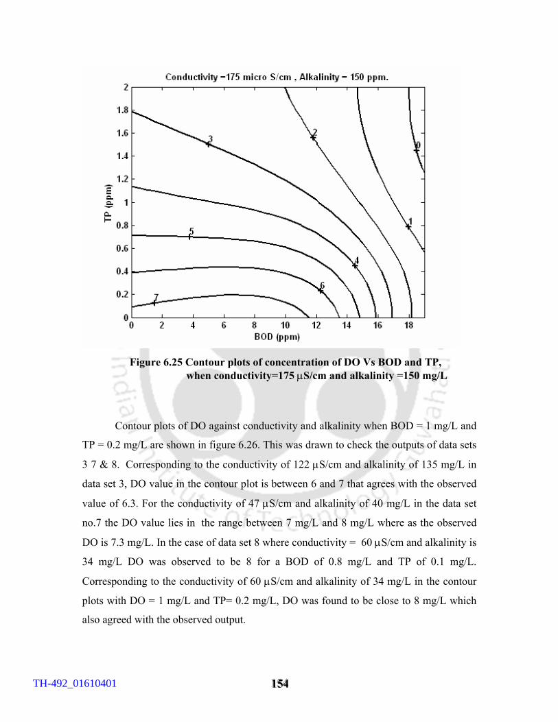
111555444

Figure 6.25 Contour plots of concentration of DO Vs BOD and TP, when conductivity=175 µS/cm and alkalinity =150 mg/L

Contour plots of DO against conductivity and alkalinity when BOD = 1 mg/L and

TP = 0.2 mg/L are shown in figure 6.26. This was drawn to check the outputs of data sets

3 7 & 8. Corresponding to the conductivity of 122 µS/cm and alkalinity of 135 mg/L in

data set 3, DO value in the contour plot is between 6 and 7 that agrees with the observed

value of 6.3. For the conductivity of 47 µS/cm and alkalinity of 40 mg/L in the data set

no.7 the DO value lies in the range between 7 mg/L and 8 mg/L where as the observed

DO is 7.3 mg/L. In the case of data set 8 where conductivity = 60 µS/cm and alkalinity is

34 mg/L DO was observed to be 8 for a BOD of 0.8 mg/L and TP of 0.1 mg/L.

Corresponding to the conductivity of 60 µS/cm and alkalinity of 34 mg/L in the contour

plots with DO = 1 mg/L and TP= 0.2 mg/L, DO was found to be close to 8 mg/L which

also agreed with the observed output.

TH-492_01610401

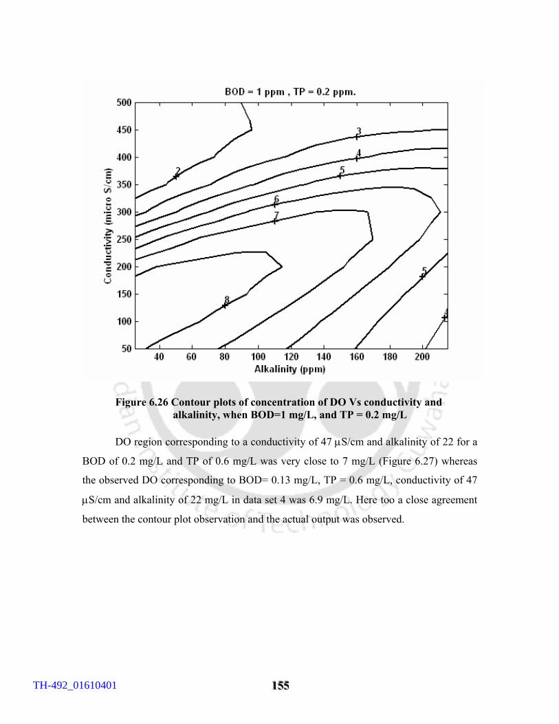
111555555

Figure 6.26 Contour plots of concentration of DO Vs conductivity and alkalinity, when BOD=1 mg/L, and TP = 0.2 mg/L

DO region corresponding to a conductivity of 47 µS/cm and alkalinity of 22 for a

BOD of 0.2 mg/L and TP of 0.6 mg/L was very close to 7 mg/L (Figure 6.27) whereas

the observed DO corresponding to BOD= 0.13 mg/L, TP = 0.6 mg/L, conductivity of 47

µS/cm and alkalinity of 22 mg/L in data set 4 was 6.9 mg/L. Here too a close agreement

between the contour plot observation and the actual output was observed.

TH-492_01610401

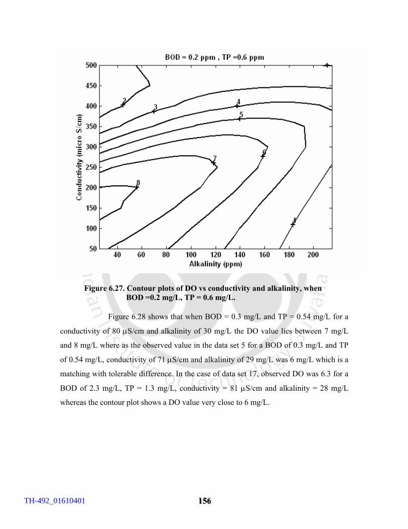
111555666

Figure 6.27. Contour plots of DO vs conductivity and alkalinity, when

BOD =0.2 mg/L, TP = 0.6 mg/L. Figure 6.28 shows that when BOD = 0.3 mg/L and TP = 0.54 mg/L for a

conductivity of 80 µS/cm and alkalinity of 30 mg/L the DO value lies between 7 mg/L

and 8 mg/L where as the observed value in the data set 5 for a BOD of 0.3 mg/L and TP

of 0.54 mg/L, conductivity of 71 µS/cm and alkalinity of 29 mg/L was 6 mg/L which is a

matching with tolerable difference. In the case of data set 17, observed DO was 6.3 for a

BOD of 2.3 mg/L, TP = 1.3 mg/L, conductivity = 81 µS/cm and alkalinity = 28 mg/L

whereas the contour plot shows a DO value very close to 6 mg/L.

TH-492_01610401

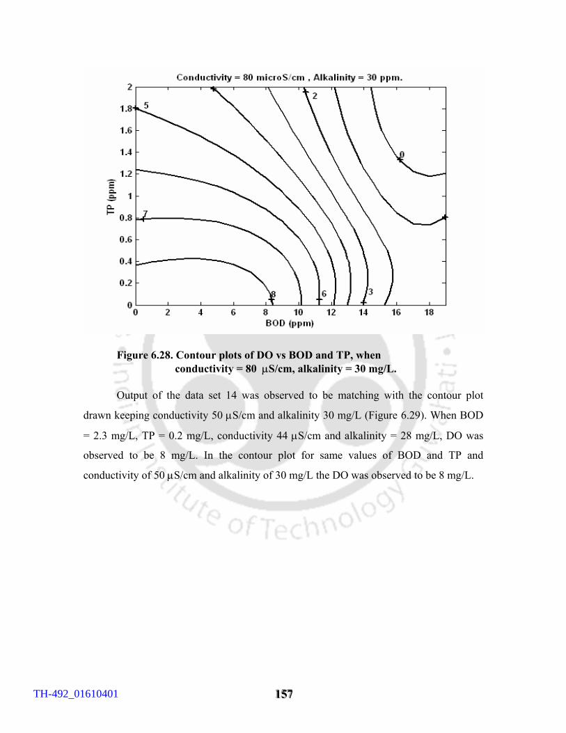
111555777

Figure 6.28. Contour plots of DO vs BOD and TP, when conductivity = 80 µS/cm, alkalinity = 30 mg/L. Output of the data set 14 was observed to be matching with the contour plot

drawn keeping conductivity 50 µS/cm and alkalinity 30 mg/L (Figure 6.29). When BOD

= 2.3 mg/L, TP = 0.2 mg/L, conductivity 44 µS/cm and alkalinity = 28 mg/L, DO was

observed to be 8 mg/L. In the contour plot for same values of BOD and TP and

conductivity of 50 µS/cm and alkalinity of 30 mg/L the DO was observed to be 8 mg/L.

TH-492_01610401

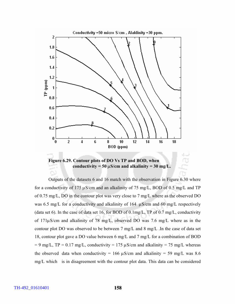
111555888

Figure 6.29. Contour plots of DO Vs TP and BOD, when conductivity = 50 µS/cm and alkalinity = 30 mg/L.

Outputs of the datasets 6 and 16 match with the observation in Figure 6.30 where

for a conductivity of 175 µS/cm and an alkalinity of 75 mg/L, BOD of 0.5 mg/L and TP

of 0.75 mg/L, DO in the contour plot was very close to 7 mg/L where as the observed DO

was 6.5 mg/L for a conductivity and alkalinity of 164 µS/cm and 60 mg/L respectively

(data set 6). In the case of data set 16, for BOD of 0.1mg/L, TP of 0.7 mg/L, conductivity

of 171µS/cm and alkalinity of 78 mg/L, observed DO was 7.6 mg/L where as in the contour plot DO was observed to be between 7 mg/L and 8 mg/L .In the case of data set

18, contour plot gave a DO value between 6 mg/L and 7 mg/L for a combination of BOD

= 9 mg/L, TP = 0.17 mg/L, conductivity = 175 µS/cm and alkalinity = 75 mg/L whereas

the observed data when conductivity = 166 µS/cm and alkalinity = 59 mg/L was 8.6

mg/L which is in disagreement with the contour plot data. This data can be considered

TH-492_01610401

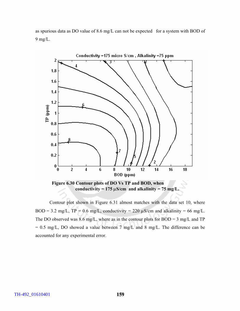
111555999

as spurious data as DO value of 8.6 mg/L can not be expected for a system with BOD of

9 mg/L.

Figure 6.30 Contour plots of DO Vs TP and BOD, when conductivity = 175 µS/cm and alkalinity = 75 mg/L.

Contour plot shown in Figure 6.31 almost matches with the data set 10, where

BOD = 3.2 mg/L, TP = 0.6 mg/L, conductivity = 220 µS/cm and alkalinity = 66 mg/L.

The DO observed was 8.6 mg/L, where as in the contour plots for BOD = 3 mg/L and TP

= 0.5 mg/L, DO showed a value between 7 mg/L and 8 mg/L. The difference can be

accounted for any experimental error.

TH-492_01610401

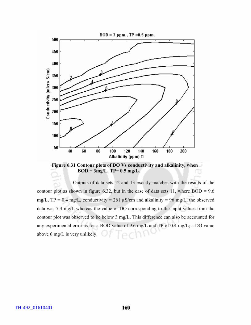
111666000

Figure 6.31 Contour plots of DO Vs conductivity and alkalinity, when BOD = 3mg/L, TP= 0.5 mg/L.

Outputs of data sets 12 and 13 exactly matches with the results of the

contour plot as shown in figure 6.32, but in the case of data sets 11, where BOD = 9.6

mg/L, TP = 0.4 mg/L, conductivity = 261 µS/cm and alkalinity = 96 mg/L, the observed

data was 7.3 mg/L whereas the value of DO corresponding to the input values from the

contour plot was observed to be below 3 mg/L. This difference can also be accounted for

any experimental error as for a BOD value of 9.6 mg/L and TP of 0.4 mg/L; a DO value

above 6 mg/L is very unlikely.

TH-492_01610401

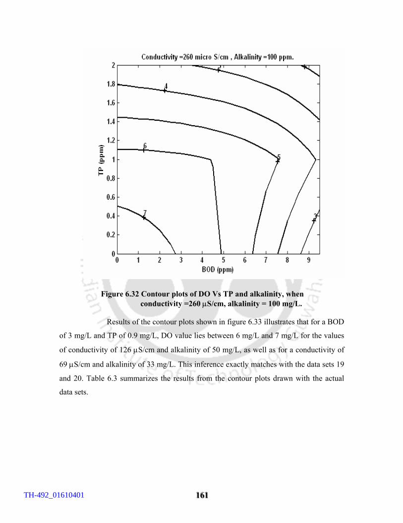
111666111

Figure 6.32 Contour plots of DO Vs TP and alkalinity, when conductivity =260 µS/cm, alkalinity = 100 mg/L. Results of the contour plots shown in figure 6.33 illustrates that for a BOD

of 3 mg/L and TP of 0.9 mg/L, DO value lies between 6 mg/L and 7 mg/L for the values

of conductivity of 126 µS/cm and alkalinity of 50 mg/L, as well as for a conductivity of

69 µS/cm and alkalinity of 33 mg/L. This inference exactly matches with the data sets 19

and 20. Table 6.3 summarizes the results from the contour plots drawn with the actual

data sets.

TH-492_01610401

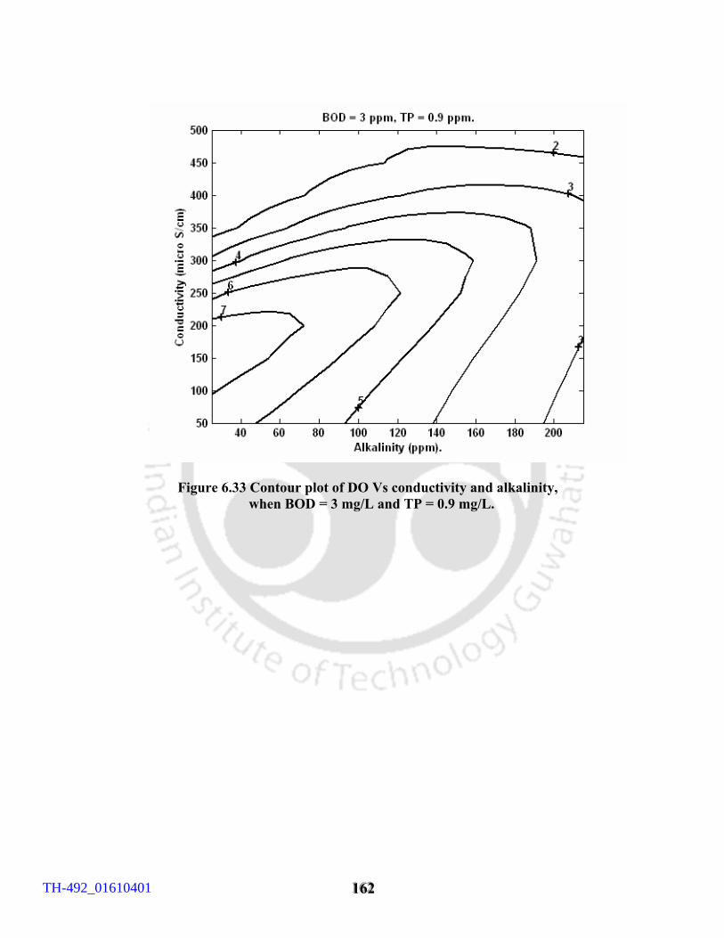
111666222

Figure 6.33 Contour plot of DO Vs conductivity and alkalinity, when BOD = 3 mg/L and TP = 0.9 mg/L.

TH-492_01610401

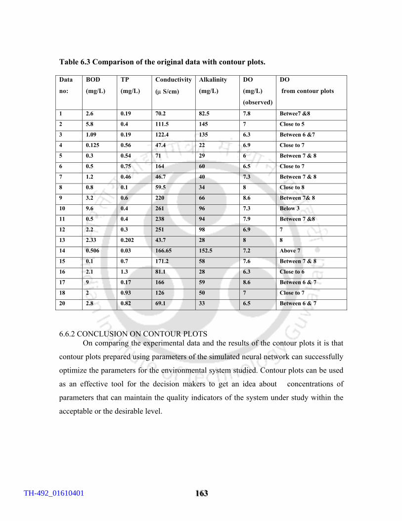
111666333

Table 6.3 Comparison of the original data with contour plots. Data

no:

BOD

(mg/L)

TP

(mg/L)

Conductivity

(µ S/cm)

Alkalinity

(mg/L)

DO

(mg/L)

(observed)

DO

from contour plots

1 2.6 0.19 70.2 82.5 7.8 Betwee7 &8

2 5.8 0.4 111.5 145 7 Close to 5

3 1.09 0.19 122.4 135 6.3 Between 6 &7

4 0.125 0.56 47.4 22 6.9 Close to 7

5 0.3 0.54 71 29 6 Between 7 & 8

6 0.5 0.75 164 60 6.5 Close to 7

7 1.2 0.46 46.7 40 7.3 Between 7 & 8

8 0.8 0.1 59.5 34 8 Close to 8

9 3.2 0.6 220 66 8.6 Between 7& 8

10 9.6 0.4 261 96 7.3 Below 3

11 0.5 0.4 238 94 7.9 Between 7 &8

12 2.2 0.3 251 98 6.9 7

13 2.33 0.202 43.7 28 8 8

14 0.506 0.03 166.65 152.5 7.2 Above 7

15 0.1 0.7 171.2 58 7.6 Between 7 & 8

16 2.1 1.3 81.1 28 6.3 Close to 6

17 9 0.17 166 59 8.6 Between 6 & 7

18 2 0.93 126 50 7 Close to 7

20 2.8 0.82 69.1 33 6.5 Between 6 & 7

6.6.2 CONCLUSION ON CONTOUR PLOTS

On comparing the experimental data and the results of the contour plots it is that

contour plots prepared using parameters of the simulated neural network can successfully

optimize the parameters for the environmental system studied. Contour plots can be used

as an effective tool for the decision makers to get an idea about concentrations of

parameters that can maintain the quality indicators of the system under study within the

acceptable or the desirable level.

TH-492_01610401

111666444

CHAPTER SEVEN MAJOR CONCLUSIONS

The generalized conclusions of the present work derived from chapter 4 and chapter 6 are

as follows:

• From the three models studied viz: The fuzzy rule based model, multiple linear

regression and the artificial neural network model, for prediction of dissolved oxygen,

which is an important water quality indicator, artificial neural network model is found

to be the most appropriate model.

• A relationship was developed connecting BOD, TP, conductivity and alkalinity with

dissolved oxygen in the system studied using artificial neural network model. From

this work, successful prediction of dissolved oxygen from a small set of physical

chemical and biological measurements, by artificial neural network model is

established.

• Selection of input variables for the ANN models based on the correlation coefficients

proved to be a reliable method.

• Explanatory capacity of the ANN model, apart from its predictive quality in ecology,

was proved by the satisfactory results obtained from the sensitivity analysis. As the

environment is composed of many characteristics acting together, considering

variable interaction proved to have meaning than finding the contribution of single

variable. Thus by means of quantitative approach like partial derivative method it is

possible to identify individual and interacting contributions of predictor variables in

ANN model.

• Contour plots proved to be efficient tools for optimizing the parameters to maintain

the system safe. For optimizing the variables of an ecosystem ranges of values are to

be obtained. Successful optimization of the variables could be arrived at by making

use of contour plots.

• Water quality of the Bharalu tributary was found to be generally poor, with

significant seasonal and spatial variations. Dissolved oxygen, was observed to be

either absent or very low in several locations irrespective of the season.

TH-492_01610401

111666555

• Analysis results indicated the presence of excess amount of decomposed organic

matter, leaching from phosphorus rich rock, human and animal waste, land and its

vegetation along the middle reach of the system under study. Excess growth of

aquatic weeds resulted in settled organic load and silt accumulation that could have

resulted in high sediment oxygen demand and respiration by biomass in the nights

adding to the stress on DO which made the system deficient in dissolved oxygen.

Desilting followed by implementing proper land use management, drainage system

and waste disposal are the effective remedial measures to be taken for the system

studied.

TH-492_01610401

111666666

SCOPE FOR FUTURE RESEARCH

• INFLUENCE OF SOD ON DISSOLVED OXYGEN OF THE WATER

COLUMN It is understood from the study that Oxygen depletion in the river

ecosystem can be attributed to a variable combination of biochemical oxygen

demand, total phosphorus, conductivity and alkalinity. Combination of

conductivity with total phosphorus and bio chemical oxygen demand was

observed to be the most contributing. Sediment can provide important storage

capacity for nutrients and there is a possibility that in nutrient rich shallow water

bodies sediment oxygen demand can be substantial due to decayed aquatic weeds

and other organic matter. Hence there is a scope for further studies in using data

ANN model in the prediction of dissolved oxygen budget of a water body

including sediment oxygen demand and study its influence.

• INCLUSION OF HYDROLOGIC PARAMETERS

Inclusion of hydrologic parameters like discharge, depth, velocity, along

with water quality variables as input parameters so as to get a complete picture of

water quality prediction of a particular environmental system. Developing such a

model makes it feasible to transfer the model to a different environmental system.

• FORMULATION OF A FUZZY NEURAL NETWORK MODEL FOR

WATER QUALITY PREDICTION

If the data sets are fuzzified and fed to the neural network instead of

feeding as such as the input variable more better generalization can be expected

and that seems to be a promising research in the future study.

TH-492_01610401

111666777

REFERENCES

Abebe, A.J., Solomatine,D.P., Venneker, R.G.W., (2000). Application of adaptive fuzzy

rule-based models for reconstruction of missing precipitation events, Hydrological

sciences journal, 45 (3), 425-436.

Adriaenssens,V., Goethals,P.L.M., de Pauw,N., (2006). Fuzzy knowledge-based models for

prediction of Asellus and Gammarus in watercourses in Flanders (Belgium),

Ecological modelling ,195 (1-2),3-10.

Adriaenssens, V., de Baets, B., Goethals, P.L.M., de Pauw, N., (2004). Review- Fuzzy

rule- based models for decision support in ecosystem Management, The Science of

the Total Environment, 319 , 1–12.

Almasril, M.N., Kalurachchi,J.J., (2005). Modular neural networks to predict the nitrate

distribution in ground water using the on-ground nitrogen loading and recharge

data, Environmental Modelling & Software, 20 , 851-871.

Altunkaynak, A.U., Ozger, M., Akmaksi, M.C., (2005). Water consumption prediction of

Istanbul city by using fuzzy logic approach. Water resources management,19, 641-

654.

Alvisi, S., Mascellani,G., Franchini, M.,B’ardossi ,A., (2006).Water level forecasting

through fuzzy logic and artificial neural network approaches, Hydrology and earth

system sciences, 10, 1-17.

APHA, 1998.Standard methods for examination of water and waste water .20th edition;

prepared and published jointly by:American Public Health Association

(APHA),American Water Works Association (AWWA),Water Pollution Control

Federation (WPCF), New York.

Basma, A.A., Kallas, N., (2004). Modeling soil collapse by artificial neural network.

(technical note).Geotechnical and geological engineering .22,427-438.

Bellos, D., Sawidis T., 2005. Chemical pollution monitoring of the River Pinios (Thessalia

–greece), Journal of Environmental Management, 76, 282-292.

TH-492_01610401

111666888

Brien,G., Chandramouli,V., Neelakantan, T.R.,Lingireddy,S., Girones,R., Lees,D., Allard,

A.,Vantarakis,A., (2005). Applied and environmental microbiology, 71(9),5244-

5253.

Broekhoven, E.V., Adriaenssens, V., De Baets, B., Verdonschot, P.F.M., (2006), Fuzzy

rule base macroinvertebrate habitat suitability models for running waters,

Ecological modelling, 198,71-84.

Burien, S.J., Durrance, S.R., Nix, S.J., Pitt, R.E., 2001. Training artificial neural network to

perform rainfall disaggregation. Journal of Hydrologic Engineering, 6(1), 43-51.

Buzas, K.,(2001).Use of fuzzy model to estimate nutrient loads from scarce

observations.Water Science and Technology, 43,(7), 257-264.

Castane, P.M., Rovedatti, M.G., Topalian, M.L., (2006). Spatial ad temporal trends of

physicochemical parameters in the water of the Reconquista River (Buenos Aires

,Argentina).Environmental monitoring and assessment .117,135-144.

Chen, D., Hare, S.R., (2006). Neural network and fuzzy logic models for pacific halibut

recruitment analysis, Ecological modeling, 195(1-2), 11-19.

Chen, Q., Mynett, A.E., (2003). Integration of data mining techniques and heuristic

knowledge in fuzzy logic modelling of eutrophication in Taihu Lake, Ecological

Modelling, 162 , 55–67.

Chau, K.W., (2006). A review on integration of artificial intelligence into water quality

modeling. Marine Pollution Bulletin, 52, 726-733.

Cox, B. A., (2003). A review of dissolved oxygen modeling techniques for lowland rivers.

The Science of the Total Environment, 314-316, 303-334.

Daliakopoulosa, I, N., Coulibalya, P., Tsanis, I.K., (2005). Groundwater level forecasting

using artificial neural networks. Journal of Hydrology, 209, 229-240.

Dimopoulos, Y., Bourret, P., Lek, S., (1995). Use of some sensitivity criteria for choosing

networks with good generalization ability. Neural Processing Letters 2, 1-4.

Drolc, A., Koncan, J.Z., (1996). Water quality modeling of the river Sava, Slovenia. Water

research,30 (11), 2587-2592.

de Vlaming,V., DiGiorgio, C., Fong,S.,deanovic, L.A.,de la Paz Carpio-

Obeso,M.D.,miller,J.L ., (2004). Irrigation runoff insecticide pollution of rivers in

the Imperial valley , California, USA. Environmental Pollution, 132, 213-229.

TH-492_01610401

111666999

Engin,G.O., Demir,I., Engin,S.N., (2005). Determination of the relationship between

sewage odour and BOD by neural networks,. Environmental Modelling & Software,

20, 843-850.

Esquerre ,K.P.O., Seborg ,D.E., Mori, M., Bruns,R.E., (2004). Application of steady state

and dynamic modeling for the prediction of the BOD of an aerated lagoon at a pulp

and paper mill- Part II. Nonlinear approaches, Chemical Engineering Journal

105,61–69.

Fatoki,O.S., Gogwana,P .,Ogunfowokan, A.O., (2003). Pollution assessment in Keiskamma

river and in the impoundment downstream. Water SA, 29(2), 183-187.

Freitas, H., Diamond, M., Semkin, R., Grigor, D.,(1997). Contaminant fate in high arctic

lakes: development and application of a mass balance model. The Science of the

Total Environment, 201,171-187.

Gevrey, M., Dimopoulos, I., Lek S., (2003). Review and comparison of methods to study

the contribution of variables in artificial neural network models. Ecological

Modeling, 160, 249-/264.

Gevrey, M., Dimopoulos, I., Lek S., (2006). Two-way interaction of input variables in the

sensitivity analysis of neural network models. Ecological Modeling, 195, 43-50.

Gibbs J., (1972). Water chemistry of Amazon River. Geochim, Cosmochim. Acta, 36,

1061-1066.

Giri, B.S., Karimi, I.A., Ray, M.B., (2001). Modeling and Monte Carlo simulation of

TCDD transport in a river. Water Research, 35(5), 1263-1279.

Goswami, D.C., Das, P.J., (2003). The Brahmaputra River, India: the ecohydrological

context of water use in one of world’s most unique river system. Ecologist Asia,

11(1) 9-14.

Gumrah, F., OZ, B., Guler, B., Evin, S., (2000). The application of artificial neural network

for the prediction of water quality of polluted aquifer. Water, Air, and Soil Pollution

119: 275–294.

Gorchev, H.G., (1996). Chlorine in water disinfection. Pure & Appl. Chem., 69(9), 1731-

1735.

Ha H, Michael K. Stenstrom., (2003). Identification of land use with water quality data in

storm water using a neural network, Water Research, 37, 4222–4230.

TH-492_01610401

111777000

Hanson, J.D., Rojas, K.W., Shaffer, M.J., (1999). Calibrating the root zone water quality

model. Agronomy Journal, 91,171-177.

Isidori, M., Lavorgna, M., Nardelli, A., Parrella, A., (2004). Integrated environmental

assessment of Volturno River in South Italy. Science of the Total Environment,

327, 123–134.

Izonfuo, L.W.A., Bariweni, A.P., (2001). The effect of urban runoff water and human

activities on some physico-chemical parameters of the Epic Creek in the Niger

Delta. Journal of Applied Science and environmental Management, 5(1), 47-55.

Judova, P., Jansky, B., (2005). Water quality in rural areas of the Czech republic: Key

study Slapanka River catchment. Limnologica, 35,160-168.

Kaloudis, S., Tocatlidou, A., Lorentzos, N.A., Sideridis, A.B., Karteris, M.,(2005).

Assessing Wildfire Destruction Danger: a Decision Support System Incorporating

Uncertainty, Ecological Modeling, 181, 25–38.

Karnakar, S., Mujumdar, P.P., (2006). Grey fuzzy optimization model for water quality

management of a river system, Advances in Water Resources, 29, 1088–1105.

Karul, C., Soyupak, S., Cilesiz, A, F., Akbay, N., Germen, E., (2000). Case studies on the

use of neural networks in eutrophication modeling. Ecological Modelling, 134,

145–152.

Lee, C.S., Chang, S.P., (2005), Interactive fuzzy optimization for an economic and

environmental balance in a river system, Water Research, 39, 221–231.

Lek, S., Guiresse, M., Giraudel, J.L., (1999). Predicting stream nitrogen concentration from

watershed features using Neural Networks. Wat. Res. 33(16), 3469-3478.

Lischeid, G., (2001), Investigating short-term dynamics and long-term trends of SO4 in the

runoff of a forested catchment using artificial neural networks. Journal of

Hydrology, 243, 31–42.

Lourakis,M., Argyros, A., (2005). Is Levenberg-Marquardt the Most Efficient Optimization

Algorithm for Implementing Bundle Adjustment? Tenth IEEE International

Conference on Computer Vision (ICCV’05) Volume 2,1526-1531.

Maier, H.R ., Dandy, G.C., (1997). Modelling cyan bacteria (blue-green algae) in the River

Murray using artificial neural networks, Mathematics and Computers in Simulation,

43, 377-386.

TH-492_01610401

111777111

Maier, H.R., Morgan, N., Chow, C. W.K., (2004). Use of artificial neural networks for

predicting optimal alum doses and treated water quality parameters, Environmental

Modelling & Software 19, 485–494.

Marchini, A., Marchini, C., (2006). A fuzzy logic model to recognize ecological sectors in

the lagoon of Venice based on the benthic community, Ecological Modelling

193,105–118.

Martin, J.C., Hoggart, C., Matissa, A., (1998). Improvement priorities for sewage treatment

in Latvian small and medium sized towns. Water science and Technology, 37(8).

137-144.

Menzl, S., Stuhler, M., Benz, R., (1996). A self-adaptive computer based pH measurement

and Fuzzy –control system, Wat. Res, 30(4), 981-991.

Metternicht, G., (2001). Assessing temporal and spatial changes of salinity using fuzzy

logic, remote sensing and GIS. Foundations of an expert system, Ecological

Modelling, 144, 163–179.

MeyLiou, S., Lo, S.L., Hu, C.Y., (2003). Application of two-stage fuzzy set theory to river

quality evaluation in Taiwan, Water Research, 37, 1406–1416.

Moartar, F., Fessent, F.O., Poirel, A., (1999). pH modelling by neural networks.

Application of control and validation data series in the Middle Loire River.

Ecological Modelling, 120, 141–156.

Mohamed, A.M.O., Cote, K., (1999). Decision analysis of polluted sites Ð a fuzzy set

approach. Waste Management, 19, 519-533.

Mpimpas, H., Anagnostopoulos, P., Ganoulis, J., (2001). Modelling of water pollution in

the Thermaikos Gulf with fuzzy parameters, Ecological Modelling, 142, 91–104.

Mujumdar, P.P., Sasikumar, K., (2002). A fuzzy risk approach for seasonal water quality

management of a river system. Water Resources Research, 38, (1), doi:

10.1029/2000WR000126.

Nash, J. E., J. V. Sutcliffe., (1970), River flow forecasting through conceptual models part

1 – a discussion of principles .Journal of hydrology,10(3), 282 – 290.

Olajire, A.A., Imeokparia, F.E., (2001). Water quality assessment of Osun River.

Environmental Monitoring and Assessment, 69,17-28.

TH-492_01610401

111777222

Olden, J.D., Joy, M.K., Death, R.G.,(2004), An accurate comparison of methods for

quantifying variable importance in artificial neural networks using simulated data.

Ecological Modelling,178, 389-397.

Recknagel,F., French M., Harkonen P., Yabunaka K.I., (1997), Artificial neural network

approach for modelling and prediction of algal blooms. Ecological Modelling, 96,

11-28.

Riad, S., Mania J., Bouchaou L., Najjar Y., (2004). Rainfall-Runoff Model Using an

Artificial Neural Network Approach, Mathematical and Computer Modelling, 40,

839-846.

Rounds, S.A., (2002). Development of a neural network model for dissolved oxygen in the

Tualatin River- Oregon, in Proceedings of the Second Federal Interagency

Hydrologic Modeling Conference, Las Vegas, Nevada, July 29 –August 1, 2002:

Subcommittee on Hydrology of the Interagency Advisory Committee on Water

Information.

Sanchez, E., Colmenarejo, M.F., Vicente, J., Rubio, A., Garcia, M.G., Travieso, L., Borja,

R., (2007). Use of water quality index and dissolved oxygen deficit as simple

indicators of watersheds pollution, Ecological Indicators, 7(2), 315-328.. Sarangi, A., Singh, M., Bhattacharya, A.K., Singh, A.K., (2006). Subsurface drainage

performance study using SALTMODE and ANN models. Agricultural Water

Management, 84, 240-248.

Sasikumar, K., Mujumdar, P.P., (1998). Fuzzy optimization model for water quality

management of a river system. Journal of Water Resources Planning and

Management.124, 79-88.

Sasikumar, K., Mujumdar, P.P., (2000). Application of fuzzy probability in water quality

management of a river system. International Journal of Systems Science, 31(5),

575-591.

Scardi, M., Harding Jr, L.W., (1999). Developing an empirical model of phytoplankton

primary production: a neural network case study. Ecological modeling, 120, 213-

223.

TH-492_01610401

111777333

Schmid, B.H., Koskiaho, J., (2006). Artificial neural network modeling of dissolved

oxygen in a wetland pond: the case of Hovi, Finland. Journal of hydraulic

engineering, (ASCE), March-April, 188-192.

Sharma, V., Negi, S.C., Rudra, R.P., Yang, S., (2003). Neural networks for predicting

nitrate-nitrogen in drainage water, Agricultural Water Management, (63), 169–183.

Shresta, B.P., Duckstein, L., Stakhiv, E.Z., (1996). Fuzzy rule based modelling of reservoir

operation. Journal of water resources planning and management. (122), 263-269.

Silva, A.M.M., Sacomani L.B., (2001). Using chemical and physical parameters to define

the quality of Pardo river water (Botucatu-sp-Brazil), Water Research.35, 1609-

1616.

Silvert, W., (1997). Ecological impact classification with fuzzy sets. Ecological modeling,

96, 1-10.

Silvert, W., (2000). Fuzzy indices of environmental conditions, Ecological Modeling, 130,

111–119.

Smith, E., (2001). Pollutant concentrations of storm water and captured sediment in flood

control sumps draining an urban watershed. Wat. Res, 35(13), 3117-3126.

Smith, D.G., Maasdam, R., (1994). New Zealand’s national river water quality network1.

Design and physico chemical characterization. New Zealand journal of marine and

freshwater research.28, 19-35.

Soyupak, S., Chen, D.G., (2004). Fuzzy logic model to estimate seasonal pseudo steady

state chlorophyll-a concentrations in reservoirs, Environmental Modeling and

Assessment, 9, 51–59.

Strik, D. T. B. T. B., Domnanovic, A. M., Zani. L., Braun, R., Holubar, P., 2005.

Prediction of trace compounds of biogas from anaerobic digestion using the

MATLAB Neural Network Toolbox. Environmental Modeling & Software, 20,803-

810.

Stow, C.A., Borsuk, M.E., Stanley, D.W., (2001). Long term changes in watershed nutrient

inputs and riverine exports in the Neuse River, North Carolina, Water Res. Vol. 35,

No.6, 1489-1499.

TH-492_01610401

111777444

Svoray, T., Gaccharski, S.B.Y., Henkin, Z., Gutman, M., (2004). Assessment of

herbaceous plant habitats in water-constrained environments: predicting indirect

effects with fuzzy logic, Ecological Modelling, 180, 537–556.

Taebi A., Droste R. L., (2004). Pollution loads in urban runoff and sanitary wastewater,

Science of the Total Environment 327, 175–184.

Tayfur, G., Ozdemir, S., Singh, V.P., (2003). Fuzzy logic algorithm for runoff- induced

sediment transport from bare soil surfaces, Advances in Water Resources 26,1249–

1256.

Tsiouris, S.E., Mamolos, A.P.,Kalburtji,K.L., Alifrangis,D., (2002). The quality of runoff

water collected from a wheat field margin in Greece. Agriculture, Ecosystem and

Environment, 89,117-125.

Valver de Ramirez, M.C., de Campos Velho, H.F., Ferreira, N.J., (2005). Artificial neural

network technique for rainfall forecasting applied to the Sa˜o Paulo region, Journal

of Hydrology, 301, 146–162.

Wang, X., Homer, M., Dyer, S .D., Hull, C .W., Changming., (2005). A river water quality

model integrated with a web-based geographic information system. Journal of

Environmental Management, 75, 219–228.

Wang, H., Hondzo, M., Xu, C., Poole, V., Spacie, A., (2003). Dissolved oxygen

dynamics of streams draining an urbanized and an agricultural catchment.

Ecological Modeling, 160, 145-161.

Wei, B., Sugiura, N., Maekawa, T., (2001). Use of artificial neural network in prediction of

algal blooms, Wat. Res, 35, (8), 2022-2028.

Wilcock, R.J., (1986). Agricultural runoff: A source of water pollution in New- Zealand.

N.Z. Agricultural. Sc. 20, 98-103.

Wilcock, R.J., McBride, G.B., Nagels, J.W., Northport, G.L., (1995). Water quality in a

polluted lowland stream with chronically depressed dissolved oxygen: causes and

effects. New Zealand journal of marine and fresh water research.29, 277-288.

Woli K.P., Nagumo T., Kuramochi K., Hatano R., (2004). Evaluating river water quality

through land use analysis and N budget approaches in livestock farming areas,

Science of the Total Environment 329, 61–74.

TH-492_01610401

111777555

Zhang, Q., Stanley, S.J., (1997). Forecasting raw- water quality parameters for the North

Saskat Chewan River by neural network modeling, Wat. Res. (31), No. 9, 2340-

2350.

Zimmerman ,H.J., (1996). Fuzzy set theory and its applications, 2nd Ed.Kluwer academic

publishers, Boston .

TH-492_01610401

111777666

LIST OF PUBLICATIONS

• Pathak.N.J., Girija,T.R., C. Mahanta.,(2006). Modeling approach towards eco-

restoration strategies for some polluted tributaries of the Brahmaputra River.

(Proceedings (CD ROM) in World Environmental and Water Resources

Congress, May 15-19, 2007,Tampa, Marriott Water side, Tampa, Florida) .

• T.R.Girija., C. Mahanta ., V. Chandramouli (2007).Water Quality Assessment of

an Untreated Effluent Impacted Urban River: The Case of the Bharalu Tributary

of the Brahmaputra River, India. Environmental monitoring and assessment,

130,221-236.

• T.R.Girija, C.Mahanta. Fuzzy logic and artificial neural network approaches for

dissolved oxygen prediction. (Accepted in International Journal of Environment

and Waste Management).

• T.R.Girija, C. Mahanta and V. Chandramouli. ANN application for water quality

management of waste water predominated small rivers: The case of the Bharalu

tributary of Brahmaputra.(Communicated to The Science of the Total

Environment).

• T.R.Girija, C.Mahanta. Importance of multiple interactions of variables in

ecological modeling. (Under preparation).

TH-492_01610401

water quality modeling in an untreated effluent dominated

Documents