week 3: monopoly and duopoly - university of warwick · introductionmonopolycournot...

Introduction Monopoly Cournot Duopoly Bertrand Summary

Week 3:Monopoly and Duopoly

Dr Daniel Sgroi

Reading: 1. Osborne Sections 3.1 and 3.2;2. Snyder & Nicholson, chapters 14 and 15;

3. Sydsæter & Hammond,Essential Mathematics for Economics Analysis, Section 4.6.

With thanks to Peter J. Hammond.

EC202, University of Warwick, Term 2 1 of 34


Outline

1. Monopoly

2. Cournot’s model of quantity competition

3. Bertrand’s model of price competition



Cost, Demand and Revenue

Consider a firm that is the only seller of what it produces.Example: a patented medicine, whose supplier enjoys a monopoly.

Assume the monopolist’s total costs are given bythe quadratic function C = αQ + βQ2 of its output level Q ≥ 0,where α and β are positive constants.

For each Q, its selling price P is assumed to be determinedby the linear “inverse” demand function P = a− bQ for Q ≥ 0,where a and b are constants with a > 0 and b ≥ 0.

So for any nonnegative Q, total revenue R is given bythe quadratic function R = PQ = (a− bQ)Q.As a function of output Q, profit is given by

π(Q) = R −C = (a− bQ)Q −αQ −βQ2 = (a−α)Q − (b +β)Q2



Profit Maximizing Quantity

Completing the square (no need for calculus!),we have π(Q) = πM − (b + β)(Q − QM)2, where

QM =a− α

2(b + β)and πM =

(a− α)2

4(b + β)

So the monopolist has a profit maximum at Q = QM ,with maximized profit equal to πM .The monopoly price is

PM = a− bQM = a− ba− α

2(b + β)=

b(a + α) + 2aβ

2(b + β)

This is valid if a > α;if a ≤ α, the firm will not produce,but will have QM = 0 and πM = 0.The two cases are illustrated in the next two slides.



Positive Output

108 C H A P T E R 4 / F U N C T I O N S O F O N E V A R I A B L E

Solution: Using formula (5) we find that profit is maximized at

Q = Q! = " 100

2!

" 52

" = 20 with !! = !(Q!) = " 1002

4!

" 52

" = 1000

This example is a special case of the monopoly problem studied in the next example.

E X A M P L E 4 (A Monopoly Problem) Consider a firm that is the only seller of the commodity itproduces, possibly a patented medicine, and so enjoys a monopoly. The total costs of themonopolist are assumed to be given by the quadratic function

C = "Q + #Q2, Q # 0

of its output level Q, where " and # are positive constants. For each Q, the price P at whichit can sell its output is assumed to be determined from the linear “inverse” demand function

P = a " bQ, Q # 0

where a and b are constants with a > 0 and b # 0. So for any nonnegative Q, the totalrevenue R is given by the quadratic function

R = PQ = (a " bQ)Q

and profit by the quadratic function

!(Q) = R " C = (a " bQ)Q " "Q " #Q2 = (a " ")Q " (b + #)Q2

The monopolist’s objective is to maximize ! = !(Q). By using (5) above, we see that thereis a maximum of ! (for the monopolist M) at

QM = a " "

2(b + #)with !M = (a " ")2

4(b + #)(!)

This is valid if a > "; if a $ ", the firm will not produce, but will have QM = 0 and!M = 0. The two cases are illustrated in Figs. 2 and 3. In Fig. 3, the part of the parabola tothe left of Q = 0 is dashed, because it is not really relevant given the natural requirementthat Q # 0. The price and cost associated with QM in (!) can be found by routine algebra.

!

QQM 2QM

!

Q

QM

Figure 2 The profit function, a > " Figure 3 The profit function, a $ "Optimal output is positive if a > α.



Zero Output

108 C H A P T E R 4 / F U N C T I O N S O F O N E V A R I A B L E

Solution: Using formula (5) we find that profit is maximized at

Q = Q! = " 100

2!

" 52

" = 20 with !! = !(Q!) = " 1002

4!

" 52

" = 1000

This example is a special case of the monopoly problem studied in the next example.

E X A M P L E 4 (A Monopoly Problem) Consider a firm that is the only seller of the commodity itproduces, possibly a patented medicine, and so enjoys a monopoly. The total costs of themonopolist are assumed to be given by the quadratic function

C = "Q + #Q2, Q # 0

of its output level Q, where " and # are positive constants. For each Q, the price P at whichit can sell its output is assumed to be determined from the linear “inverse” demand function

P = a " bQ, Q # 0

where a and b are constants with a > 0 and b # 0. So for any nonnegative Q, the totalrevenue R is given by the quadratic function

R = PQ = (a " bQ)Q

and profit by the quadratic function

!(Q) = R " C = (a " bQ)Q " "Q " #Q2 = (a " ")Q " (b + #)Q2

The monopolist’s objective is to maximize ! = !(Q). By using (5) above, we see that thereis a maximum of ! (for the monopolist M) at

QM = a " "

2(b + #)with !M = (a " ")2

4(b + #)(!)

This is valid if a > "; if a $ ", the firm will not produce, but will have QM = 0 and!M = 0. The two cases are illustrated in Figs. 2 and 3. In Fig. 3, the part of the parabola tothe left of Q = 0 is dashed, because it is not really relevant given the natural requirementthat Q # 0. The price and cost associated with QM in (!) can be found by routine algebra.

!

QQM 2QM

!

Q

QM

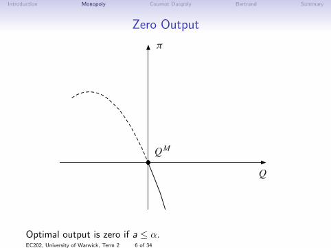
Figure 2 The profit function, a > " Figure 3 The profit function, a $ "Optimal output is zero if a ≤ α.EC202, University of Warwick, Term 2 6 of 34


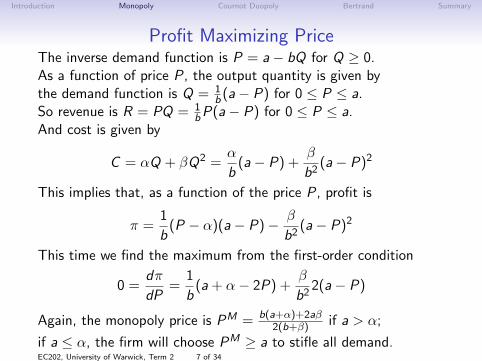
Profit Maximizing PriceThe inverse demand function is P = a− bQ for Q ≥ 0.As a function of price P, the output quantity is given bythe demand function is Q = 1

b (a− P) for 0 ≤ P ≤ a.So revenue is R = PQ = 1

bP(a− P) for 0 ≤ P ≤ a.And cost is given by

C = αQ + βQ2 =α

b(a− P) +

β

b2(a− P)2

This implies that, as a function of the price P, profit is

π =1

b(P − α)(a− P)− β

b2(a− P)2

This time we find the maximum from the first-order condition

0 =dπ

dP=

1

b(a + α− 2P) +

β

b22(a− P)

Again, the monopoly price is PM = b(a+α)+2aβ2(b+β) if a > α;

if a ≤ α, the firm will choose PM ≥ a to stifle all demand.EC202, University of Warwick, Term 2 7 of 34


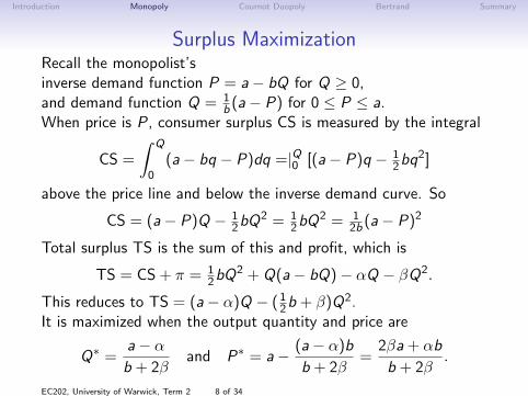
Surplus MaximizationRecall the monopolist’sinverse demand function P = a− bQ for Q ≥ 0,and demand function Q = 1

b (a− P) for 0 ≤ P ≤ a.When price is P, consumer surplus CS is measured by the integral

CS =

∫ Q

0(a− bq − P)dq =|Q0 [(a− P)q − 1

2bq2]

above the price line and below the inverse demand curve. So

CS = (a− P)Q − 12bQ

2 = 12bQ

2 = 12b (a− P)2

Total surplus TS is the sum of this and profit, which is

TS = CS + π = 12bQ

2 + Q(a− bQ)− αQ − βQ2.

This reduces to TS = (a− α)Q − (12b + β)Q2.It is maximized when the output quantity and price are

Q∗ =a− αb + 2β

and P∗ = a− (a− α)b

b + 2β=

2βa + αb

b + 2β.



Surplus Diagram

Surplus is maximized when Q = Q∗ =a− αb + 2β

.

0

0

α

− bQ∗

a

P

Q∗ a/b Q

P = MC = α+ 2βQ

P = P ∗

P = a− bQ

1



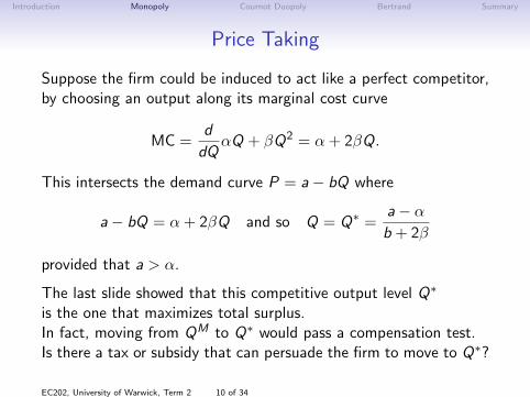
Price Taking

Suppose the firm could be induced to act like a perfect competitor,by choosing an output along its marginal cost curve

MC =d

dQαQ + βQ2 = α + 2βQ.

This intersects the demand curve P = a− bQ where

a− bQ = α + 2βQ and so Q = Q∗ =a− αb + 2β

provided that a > α.

The last slide showed that this competitive output level Q∗

is the one that maximizes total surplus.In fact, moving from QM to Q∗ would pass a compensation test.Is there a tax or subsidy that can persuade the firm to move to Q∗?



Taxing Monopoly Output

Suppose the monopolist is chargeda specific tax of t per unit of output.The tax payment tQ is extra cost, so the new total cost function is

C = αQ + βQ2 + tQ = (α + t)Q + βQ2

To find the new profit maximizing quantity choice QMt ,

carry out the same calculations as before,but with α replaced by α + t; this gives

QMt =

a− α− t

2(b + β)if a > α + t

but QMt = 0 if a ≤ α + t.



Subsidizing Monopoly Output

The objective of remedial policy should be to maximize surplusby having the firm choose QM

t = Q∗. This requires

QMt =

a− α− t

2(b + β)= Q∗ =

a− αb + 2β

provided that a > α, with QMt = 0 if a ≤ α. Clearing fractions,

we obtain (b + 2β)(a− α− t) = 2(b + β)(a− α) whose solution is

t∗ = −(a− α)b

b + 2β< 0 if a > α

So it is desirable to subsidize the monopolist’s outputin order to encourage additional production.



Taxing Monopoly Profits

Subsidizing monopolists is usually felt to be unjust,and many additional complications need to be considered carefullybefore formulating a desirable policy for dealing with monopolists.

Still the previous analysis suggeststhat if justice requires lowering a monopolist’s price or profit,this is much better done directly than by taxing output.



Cournot Duopoly Example: Costs

Suppose two identical firms, labelled 1 and 2,sell bottled mineral water.Assume that there are no fixed costs,but each firm i ’s variable costs of producing quantity qiare given by the quadratic cost function

ci (qi ) = q2i for i ∈ {1, 2}.



Competitive Price-Taking

The assumption in a competitive environmentis that each firm will take a market price p as given,believing that its behaviour cannot influence the market price.COMMENT: Or will act as if it so believes.

Each firm i chooses a quantity qi to maximize its profits.So the firms face the identical profit maximization problem

maxqi

πi (qi ) := p · qi − ci (qi ) = p · qi − q2i .

Note that π′i (qi ) = ddqi

(p · qi − q2i ) = p − 2qi

so π′i (qi ) > 0⇐⇒ qi <12p and π′i (qi ) < 0⇐⇒ qi >

12p.

Therefore, each firm will choose its supplyas a function qi (p) = 1

2p of the price p.



Elementary Economics Interpretation

Economics students should know thatin a perfectly competitive market,a firm’s marginal cost as a function of its quantitywill represent its supply curve.

Here each firm i ’s marginal costis the derivative C ′i (qi ) = 2qi of its cost function.Equating marginal cost to price gives p = 2qi or qi (p) = 1

2p,exactly the supply function derived above.



Market Demand

Suppose the total consumer demand is given by

p(q) = 100− q,

where q represents the total quantity demanded,and p(q) is the resulting price consumers are willing to pay.Alternatively, we can write market demandas a function qD = 100− p of the price.

Note: Recall that, following Cournot himself (1838),economists often “invert” the demand functionand write price as a function of quantity,rather than quantity as a function of price.This allows for some nice graphical analyses that we will also use.



Price-Taking Equilibrium I

The price-taking equilibrium occurs at a price pwhere the total output q1(p) + q2(p) of both firms’ outputsequals the demand qD(p) at the same price.Algebraically this is trivial:we need to find a price that solves

q1(p) + q2(p) = 2 · 1

2p = qD(p) = 100− p.

This yields p = 50, and each firm produces qi = 12p = 25.



Price-Taking Equilibrium II

For those used to derive the competitive equilibriumgraphically from supply and demand curves,we add up the two firms’ supply curves “horizontally”,and the equilibriumis where total supply intersects the demand curve.

In this “competitive” price-taking equilibriumeach firm maximizes profitswhen it takes the equilibrium price p = 50 as givenand chooses qi = 1

2p = 25.

Then each firm’s profitsare πi = 50 · 25− 252 = 1250− 625 = 625.



Price Manipulation

Suppose firm 1 becomes more sophisticatedand realizes that reducing its output will raise the market price.Specifically, suppose it produces 24 units instead of 25.For demand to equal the new restricted supply,the price must change to p(q) = 100− q = 51,where q = 24 + 25 = 49 instead of 50.Firm 1’s profits will then beπi = 51 · 24− 242 = 1224− 576 = 648 > 625.Of course, once firm 1 realizes its power over price,it should not just set q1 = 25 but look for its best choice.However, that choice depends on firm 2’s output quantity— what will that be?Clearly, firm 2 should be just as sophisticated.Thus, we have to look for a solutionthat considers both actions and counter-actionsof these rational and sophisticated (or well advised) firms.



Cournot Best Responses

Consider the Cournot duopoly gamewith inverse demand p = 100− qand cost functions ci (qi ) = ci · qi for firms i ∈ {1, 2}.Firm i ’s profit is ui (qi , qj) = (100− qi − qj) · qi − ci · qi .Given its belief that its opponent’s quantity is qj ,its best response is q∗i (qj) = max{0, 50− 1

2(qj + ci )}.A (Cournot) Nash equilibrium occursat a pair of quantities (q1, q2)that are mutual best responses.

So equilibrium requires q1 = q∗1(q2) and q2 = q∗2(q1).We must solve both these best response equations simultaneously.



Zero Cost Case

In the easy case with each ci = 0the two best response functions are q∗1(q2) = max{0, 50− 1

2q2}and q∗2(q1) = max{0, 50− 1

2q1}.These two equations imply that q∗i ≤ 50 for i = 1, 2, hencetheir solution satisfies both q∗1 = 50− 1

2q∗2 and q∗2 = 50− 1

2q∗1 .

Subtracting one equation from the othergives q∗1 − q∗2 = −1

2(q∗2 − q∗1), so q∗1 = q∗2 .The unique Cournot equilibrium is q∗1 = q∗2 = 331

3 .



Intersecting Best Responses

In the general case when each ci < 50you should draw a diagram in the q1 – q2 planeof the two best responsefunctions q∗1(q2) = max{0, 50− 1

2(q2 + c1)}and q∗2(q1) = max{0, 50− 1

2(q1 + c2)}.Part of each graph lies along the line segment q∗i = 0.The other parts are line segments joining:

1. (0, 100− c1) to (50− 12c1, 0);

2. (0, 50− 12c2) to (100− c2, 0).

The only equilibrium occurs at the intersectionof these two line segments, where qi > 0while q1 = 50− 1

2(q2 + c1) and q2 = 50− 12(q1 + c2).



Graph of Best Responses

Cournot equilibrium occurs at the intersectionof the two firms’ best response functions.

0

0

50− 12c2

100 − c1

q2

50− 12c1

100 − c2 q1

1



General Cournot Equilibrium

Finding the unique equilibrium requires solvingthe equations q1 = 50− 1

2(q2 + c1) and q2 = 50− 12(q1 + c2).

Adding the two equations impliesthat q1 + q2 = 100− 1

2(q2 + q1)− 12(c1 + c2)

and so q1 + q2 = 6623 − 1

3(c1 + c2).

Subtracting the second equation from the firstimplies that q1 − q2 = −1

2(q2 − q1)− 12(c1 − c2)

and so q1 − q2 = c2 − c1.

These equations imply that qi = 3313 + 1

3cj − 23ci for

i = 1, 2, j = 1, 2, i 6= j .

For c2 = c1 we have qi = 3313 − 1

3ci for i = 1, 2.



Bertrand Duopoly

In the Cournot model firms choose quantities,and the price adjusts to clear market demand.

Joseph Bertrand in 1883 modelled duopolywhen firms set prices and consumers choose where to purchase.

Consider the alternative game where the two firmseach post their own price for their identical goods.Assume that demand is given by p = 100− qand cost functions are ci (qi ) = ci qi for firms i ∈ {1, 2}.Assume too that 0 ≤ c1 ≤ c2 < 100.



Bertrand Competition

The firm that posts the lower priceobviously attracts all the consumers.If both prices are the same, we assumethat the market is split equally between the two firms.

First, consider what happens if firm i is a monopolist.It will choose quantity qto maximize (100− q)q − ciq = (100− ci )q − q2.The monopoly quantity is qMi = 50− 1

2ci .The corresponding price is pMi = 100− qMi = 50 + 1

2ci .

Note how ci < 100 implies that ci < 50 + 12ci = pMi for i ∈ {1, 2}.



The Bertrand Normal Form

Here is the normal form:

Players: N = {1, 2};Strategy sets: The firms i ∈ N

choose prices pi ∈ Si = [0,∞);

Payoffs: The quantities are given by

qi (pi , pj) =

100− pi if pi < pj

0 if pi > pj12(100− pi ) if pi = pj

and the payoffs by ui (pi , pj) = (pi − ci ) qi (pi , pj).



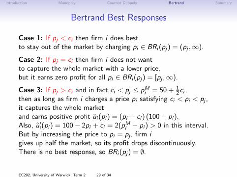
Bertrand Best Responses

Case 1: If pj < ci then firm i does bestto stay out of the market by charging pi ∈ BRi (pj) = (pj ,∞).

Case 2: If pj = ci then firm i does not wantto capture the whole market with a lower price,but it earns zero profit for all pi ∈ BRi (pj) = [pj ,∞).

Case 3: If pj > ci and in fact ci < pj ≤ pMi = 50 + 12ci ,

then as long as firm i charges a price pi satisfying ci < pi < pj ,it captures the whole marketand earns positive profit ui (pi ) = (pi − ci ) (100− pi ).Also, u′i (pi ) = 100− 2pi + ci = 2(pMi − pi ) > 0 in this interval.But by increasing the price to pi = pj , firm igives up half the market, so its profit drops discontinuously.There is no best response, so BRi (pj) = ∅.



No Profit Maximum

Firm i ’s profit is not maximized when pi = pj .

0

0

firm i’s profit

pipj pMi

bc

bc

b



More Bertrand Best Responses

Case 4: Suppose pj > pMi = 50 + 12ci > ci because ci < 100.

As long as pi < pj , profits are ui (pi ) = (pi − ci ) (100− pi ).Therefore u′i (pi ) = 100− 2pi + ci ≷ 0 as pi ≶ 50 + 1

2ci = pMi .So BRi (pj) = {pMi } = {50 + 1

2ci}.



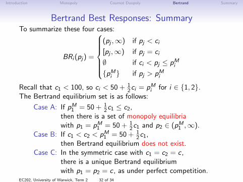
Bertrand Best Responses: SummaryTo summarize these four cases:

BRi (pj) =

(pj ,∞) if pj < ci

[pj ,∞) if pj = ci

∅ if ci < pj ≤ pMi{pMi } if pj > pMi

Recall that c1 < 100, so ci < 50 + 12ci = pMi for i ∈ {1, 2}.

The Bertrand equilibrium set is as follows:

Case A: If pM1 = 50 + 12c1 ≤ c2,

then there is a set of monopoly equilibriawith p1 = pM1 = 50 + 1

2c1 and p2 ∈ (pM1 ,∞).Case B: If c1 < c2 < pM1 = 50 + 1

2c1,then Bertrand equilibrium does not exist.

Case C: In the symmetric case with c1 = c2 = c ,there is a unique Bertrand equilibriumwith p1 = p2 = c , as under perfect competition.



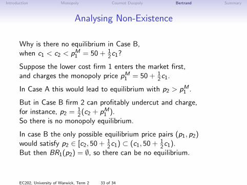
Analysing Non-Existence

Why is there no equilibrium in Case B,when c1 < c2 < pM1 = 50 + 1

2c1?

Suppose the lower cost firm 1 enters the market first,and charges the monopoly price pM1 = 50 + 1

2c1.

In Case A this would lead to equilibrium with p2 > pM1 .

But in Case B firm 2 can profitably undercut and charge,for instance, p2 = 1

2(c2 + pM1 ).So there is no monopoly equilibrium.

In case B the only possible equilibrium price pairs (p1, p2)would satisfy p2 ∈ [c2, 50 + 1

2c1) ⊂ (c1, 50 + 12c1).

But then BR1(p2) = ∅, so there can be no equilibrium.



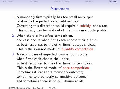
Summary

1. A monopoly firm typically has too small an outputrelative to the perfectly competitive ideal.Correcting this distortion would require a subsidy, not a tax.This subsidy can be paid out of the firm’s monopoly profits.

2. When there is imperfect competition,one case occurs when firms each choose their outputas best responses to the other firms’ output choices.This is the Cournot model of quantity competition.

3. A second case of imperfect competition occurswhen firms each choose their priceas best responses to the other firms’ price choices.This is the Bertrand model of price competition.Sometimes it leads to a monopoly outcome;sometimes to a perfectly competitive outcome;and sometimes there is no equilibrium at all.


week 3: monopoly and duopoly - university of warwick · introductionmonopolycournot...

Documents