weibull lindley distribution - statistics portugal · weibull lindley distribution authors: a....

WEIBULL lINDLEY DISTRIBUTION

Authors: A. Asgharzadeh– Department of Statistics

University of MazandaranBabolsarIran

S. Nadarajah– School of Mathematics

University of ManchesterManchester M13 9PL, UKemail: [email protected]

F. Sharafi– Department of Statistics

University of MazandaranBabolsarIran

Abstract:

• A new distribution is introduced based on compounding Lindley and Weibull distri-butions. This distribution contains Lindley and Weibull distributions as special cases.Several properties of the distribution are derived including the hazard rate function,moments, moment generating function, and Lorenz curve. An estimation procedureby the method of maximum likelihood and a simulation study to assess its perfor-mance are given. Three real data applications are presented to show that the newdistribution fits better than known generalizations of the Lindley distribution.

Key-Words:

• Lindley distribution; Maximum likelihood estimation; Weibull distribution.

AMS Subject Classification:

• Primary 62E99.

1. Introduction

The Lindley distribution was first proposed by Lindley [20] in the context offiducial and Bayesian inference. In recent years, this distribution has been studiedand generalized by several authors, see Ghitany et al. [15], Zalerzadeh and Dolati

2 A. Asgharzadeh, S. Nadarajah and F. Sharafi

[29], Ghitany et al. [14], Bakouch et al. [4], Barreto-Souza and Bakouch [5] andGhitany et al. [13].

In this paper, we introduce a new generalization of the Lindley distributionreferred to as the Weibull Lindley (WL) distribution by compounding Lindleyand Weibull distributions. The compounding approach gives new distributionsthat extend well-known families of distributions and at the same time offer moreflexibility for modeling lifetime data. The flexibility of such compound distribu-tions comes in terms of one or more hazard rate shapes, that may be decreasingor increasing or bathtub shaped or upside down bathtub shaped or unimodal.

Many recent distributions have been introduced by using a compoundingapproach. For example, Adamidis and Loukas [1] proposed a distribution by tak-ing the minimum of N independent and identical exponential random variables,where N is a geometric random variable. But this distribution allows for onlydecreasing hazard rates. Kus [18] proposed a distribution by taking the minimumof N independent and identical exponential random variables, where N is a Pois-son random variable. But this distribution also allows for only decreasing hazardrates. Barreto-Souza et al. [6] proposed a distribution by taking the minimum ofN independent and identical Weibull random variables, where N is a geometricrandom variable. But this distribution does not allow for bathtub shaped hazardrates, the most realistic hazard rates. Morais and Barreto-Souza [22] proposeda distribution by taking the minimum of N independent and identical Weibullrandom variables, where N is a power series random variable. But this distribu-tion also does not allow for bathtub shaped hazard rates. Asgharzadeh et al. [3]proposed a distribution by taking the minimum of N independent and identicalPareto type II random variables, where N is a Poisson random variable. But thisdistribution allows for only decreasing hazard rates. Silva et al. [27] proposeda distribution by taking the minimum of N independent and identical extendedWeibull random variables, where N is a power series random variable. This distri-bution does allow for bathtub shaped hazard rates, but that is expected since theextended Weibull distribution contains as particular cases many generalizationsof the Weibull distribution. Bourguignon et al. [7] proposed a distribution bytaking the minimum of N independent and identical Birnbaum-Saunders randomvariables, where N is a power series random variable. But this distribution doesnot allow for bathtub shaped hazard rates.

The WL distribution introduced here is obtained by compounding justtwo random variables (Lindley and Weibull random variables). Besides the WLdistribution has just three parameters, less than several of the distributions citedabove.

Let Y denote a Lindley random variable with parameter λ > 0 and survivalfunction G(y) = 1+λ+λy

1+λ e−λy, y > 0. Let Z denote a Weibull random variable

with parameters α > 0 and β > 0, and survival function Q(z) = e−(βz)α, z > 0.

Assume Y and Z are independent random variables. We define X = min(Y, Z)as a WL random variable and write X ∼ WL(α, β, λ). The survival function of

Weibull Lindley distribution 3

X is

F (x) = G(x)Q(x).

The cumulative distribution function (cdf) of X can be written as

F (x) = 1− 1 + λ+ λx

1 + λe−λx−(βx)

α(1.1)

for x > 0, α > 0, β ≥ 0 and λ ≥ 0. The probability density function (pdf) of Xis

f(x) =1

1 + λ

[αλ(βx)α + αβ(1 + λ)(βx)α−1 + λ2(1 + x)

]e−λx−(βx)

α(1.2)

for x > 0, α > 0, β ≥ 0 and λ ≥ 0.

Some special cases of the WL distribution are: the Weibull distributionwith parameters α and β for λ = 0; the Rayleigh distribution with parameter αfor λ = 0 and β = 2; the exponential distribution with parameter β for λ = 0and α = 1; the Lindley distribution with parameter λ for β = 0.

The WL distribution can be used very effectively for analyzing lifetimedata. Some possible motivations for the WL distribution are:

• The WL distribution accommodates different hazard rate shapes, that maybe decreasing or increasing or bathtub shaped, see Figure 2. Bathtubshaped hazard rates are very important in practice. None of the knowngeneralizations of the Lindley distribution accommodate a bathtub shapedhazard rate function.

• The WL distribution has closed form expressions for survival and hazardrate functions, which is not the case for some generalizations of the Lindleydistribution. Hence, the likelihood function for the WL distribution takesexplicit forms for ordinary type-II censored data and progressively type-IIcensored data. Hence, the WL distribution could be a suitable model toanalyse ordinary type-II censored data and progressively type-II censoreddata.

• The Lindley and Weibull distributions are special cases of the WL distri-bution.

• Suppose a system is composed of two independent components in series;let Y and Z denote their lifetimes; suppose Y is a Lindley random variableand Z is a Weibull random variable; then the lifetime of the system is aWL random variable.

• Suppose a system is composed of n independent components in series; letY,Z1, Z2, . . . , Zn−1 denote their lifetimes; suppose Y is a Lindley randomvariable and Z1, Z2, . . . , Zn−1 are identical Weibull random variables; thenthe lifetime of the system is also a WL random variable.


• The pdf of the WL distribution can be bimodal, see Figure 1. This is notthe case for the Weibull distribution or any generalization of the Lindleydistribution. So, any bimodal data set (see Figure 8 for example) cannotbe adequately modeled by any of the known generalizations of the Lindleydistribution.

• Additive hazard rates arise in many practical situations, for example, event-history analysis (Yamaguchi [28]), modeling of excess mortalities (Gail andBenichou [12], page 391), modeling of breast cancer data (Cadarso-Suarezet al. [8]), modelling of hazard rate influenced by periodic fluctuations oftemperature (Nair et al. [24], page 268), and “biologic” and “statistical” in-teractions in epidemiology (Andersen and Skrondal [2]). Hence, it is importto have distributions based on additive hazard rates. The WEL distribu-tion is the first generalization of the Lindley distribution based on additivehazard rates.

The rest of this paper is organized as follows: various mathematical prop-erties of the WL distribution are derived in Sections 2 to 4; estimation andsimulation procedures for the WL distribution are derived in Section 5; three realdata applications are illustrated in Section 6.

Some of the mathematical properties derived in Sections 2 to 4 involve in-finite series: namely, (3.1), (3.2) and (4.1). Extensive computations not reportedhere showed that the relative errors between (3.1), (3.2) and (4.1) and their ver-sions with the infinite series in each truncated at twenty did not exceed 10−20.This shows that (3.1), (3.2) and (4.1) can be computed for most practical useswith their infinite sums truncated at twenty. The computations were performedusing Maple. Maple took only a fraction of a second to compute the truncatedversions of (3.1), (3.2) and (4.1). The computational times for the truncatedversions were significantly smaller than those for the untruncated versions andthose based on numerical integration.

Throughout this paper, we report conclusions on various properties of theWL distribution: the last four paragraphs of Section 2.1 reporting conclusionson the shape of the pdf of the WL distribution; the last paragraph of Section2.2 reporting conclusions on the shape of the hazard rate function of the WLdistribution; Section 2.3 reporting conclusions on the shape of the quartiles ofthe WL distribution; the last paragraph of Section 3 reporting conclusions on themean, variance, skewness and kurtosis of the WL distribution; the last paragraphof Section 4 reporting conclusions on the Lorenz curve of the WL distribution.These conclusions are the result of extensive graphical analyses based on a widerange of parameter values (although the graphics presented here are based on afew choices of parameter values). However, we have no analytical proofs for theseconclusions.


2. Shapes

Here, we study the shapes of the pdf, (1.2), the corresponding hazard ratefunction and the corresponding quartiles. Shape properties are important becausethey allow the practitioner to see if the distribution can be fitted to a given dataset (this can be seen, for example, by comparing the shape of the histogram ofthe data with possible shapes of the pdf). Shape properties of the hazard ratefunction are useful to see if the distribution can model increasing failure rates,decreasing failure rates or bathtub shaped failure rates. Shape properties of thehazard rate function has implications, for example, to the design of safe systemsin a wide variety of applications. Quartiles are fundamental for estimation (forexample, quartile estimators) and simulation.

2.1. Shape of probability density function

We can see from (1.2) that

limx→0

f(x) =

∞, α < 1,β(1 + λ) + λ2

1 + λ, α = 1,

λ2

1 + λ, α > 1

and

f(x) ∼

λ2

1 + λxe−λx−(βx)

α, α < 1,

(β + λ)λ

1 + λxe−λx−βx, α = 1,

αβαλ

1 + λe−λx−(βx)

α, α > 1

as x→∞.

Note also that f(x) can be written as

f(x) = g(x)Q(x) + q(x)G(x),

where

g(x) =λ2(1 + x)

1 + λe−λx

and

q(x) = αβαxα−1e−(βx)α.

So, the first derivative of f(x) is

f ′(x) = g′(x)Q(x) + q′(x)G(x)− 2g(x)q(x).


Therefore, f(x) is decreasing if g′(x) < 0 and q′(x) < 0. This is possible if λ ≥ 1and α ≤ 1.

The first derivative of f(x) is

f ′(x) =e−λx−(βx)

α

1 + λ

[(1 + λ+ λx)

[αβ2(α− 1)(βx)α−2 − (αβ)2(βx)2α−2

]−2αβλ2(βx)α−1 + λ2(1− λ− λx)

].

So, the modes of f(x) at say x = x0 are the roots of

(1 + λ+ λx)[αβ2(α− 1)(βx)α−2 − (αβ)2(βx)2α−2

]= 2αβλ2(βx)α−1 − λ2(1− λ− λx).(2.1)

The roots of (2.1) are difficult to find in general. However, if β = 0 then x0 = 1−λλ ,

the mode of the Lindley distribution, for 0 < λ < 1.

0.0 0.5 1.0 1.5 2.0

0.0

0.5

1.0

1.5

x

PD

F

0.0 0.5 1.0 1.5 2.0

0.0

0.5

1.0

1.5

0.0 0.5 1.0 1.5 2.0

0.0

0.5

1.0

1.5

0.0 0.5 1.0 1.5 2.0

0.0

0.5

1.0

1.5

a = 7 & λ = 1.2a = 7 & λ = 1.4a = 7 & λ = 1.6a = 7 & λ = 1.8

0.0 0.5 1.0 1.5 2.0

0.0

0.2

0.4

0.6

0.8

1.0

1.2

x

PD

F

0.0 0.5 1.0 1.5 2.0

0.0

0.2

0.4

0.6

0.8

1.0

1.2

0.0 0.5 1.0 1.5 2.0

0.0

0.2

0.4

0.6

0.8

1.0

1.2

0.0 0.5 1.0 1.5 2.0

0.0

0.2

0.4

0.6

0.8

1.0

1.2

a = 2 & λ = 1.2a = 2 & λ = 1.4a = 2 & λ = 1.6a = 2 & λ = 1.8

Figure 1: Pdfs of the WL distribution for β = 1.

We now study (2.1) graphically. Figure 1 shows possible shapes of the pdfof the WL distribution for selected (α, β, λ).

The left plot in Figure 1 shows bimodal shapes of the pdf with a maximumfollowed by a minimum. The x coordinates of the (local minimum, local maxi-mum) are (0.395, 0.933) for λ = 1.2, (0.451, 0.921) for λ = 1.4, (0.500, 0.906) forλ = 1.6 and (0.547, 0.889) for λ = 1.8. The location of the minimum moves moreto the right with increasing values of λ. The location of the maximum movesmore to the left with increasing values of λ.


The right plot in Figure 1 shows unimodal shapes of the pdf. The x coor-dinates of the mode are 0.370 for λ = 1.2, 0.298 for λ = 1.4, 0.227 for λ = 1.6and 0.157 for λ = 1.8. The location of the mode moves more to the left withincreasing values of λ.

Monotonically decreasing shapes and monotonically decreasing shapes con-taining an inflexion point are also possible for the pdf.

In each plot, the upper tails of the pdf become lighter with increasing valuesof λ. The lower tails of the pdf become heavier with increasing values of λ.

2.2. Shape of hazard rate function

Using (1.1) and (1.2), the hazard rate function of the WL distribution canbe obtained as

h(x) =λ2(1 + x)

1 + λ+ λx+ αβ(βx)α−1.(2.2)

It is obvious that the hazard rate functions of Lindley and Weibull distributionsare contained as particular cases for β = 0 and λ = 0, respectively. Also, (2.2)can be expressed as

hX(x) = hY (x) + hZ(x),

i.e., the hazard rate function of the WL distribution is the sum of the hazard ratefunctions of Lindley and Weibull distributions. As a result, the hazard rate func-tion of the WL distribution can exhibit monotonically increasing, monotonicallydecreasing and bathtub shapes, see Figure 2.

We can see from (2.2) that

limx→0

h(x) =

∞, α < 1,

β(1 + λ) + λ2

1 + λ, α = 1,

λ2

1 + λ, α > 1

and

limx→∞

h(x) =

λ, α < 1,

λ+ β, α = 1,∞, α > 1.

Bathtub shapes of the the hazard rate function appear possible when α isclose enough to 0 or α is close enough to 1, see Figure 2. Monotonically decreasingshapes are possible for all values of α in between (i.e., in between α being close


enough to 0 and α being close enough to 1). Monotonically increasing shapes arepossible for all other values of α.

1e−04 1e−03 1e−02 1e−01 1e+00

24

68

10

x

HR

F

1e−04 1e−03 1e−02 1e−01 1e+00

24

68

10

1e−04 1e−03 1e−02 1e−01 1e+00

24

68

10

1e−04 1e−03 1e−02 1e−01 1e+00

24

68

10

a = 1e−04 & λ = 1a = 1e−04 & λ = 2a = 1e−04 & λ = 5a = 1e−04 & λ = 10

1e−04 1e−03 1e−02 1e−01 1e+00

24

68

10

x

HR

F

1e−04 1e−03 1e−02 1e−01 1e+00

24

68

10

1e−04 1e−03 1e−02 1e−01 1e+00

24

68

10

1e−04 1e−03 1e−02 1e−01 1e+00

24

68

10

a = 0.95 & λ = 1a = 0.95 & λ = 2a = 0.95 & λ = 5a = 0.95 & λ = 10

Figure 2: Hazard rate function of the WL distribution for β = 1.

2.3. Shape of quartiles

The pth quartile say xp of a WL random variable defined by F (xp) = p isthe root of

xp =1 + λ

λ

[(1− p)eλxp+(βxp)

α

− 1]

for 0 < p < 1. Numerical investigations showed that xp are monotonic decreasingfunctions of λ and monotonic increasing functions of α except for high quartiles.

3. Moment generating function and moments

The moment generating function is fundamental for computing moments,factorial moments and cumulants of a random variable. It can also be used forestimation (for example, estimation methods based on empirical moment gener-ating functions).

Moments are fundamental for any distribution. For instance, the first fourmoments can be used to describe any data fairly well. Moments are also usefulfor estimation (for example, the method of moments).


Several interesting characteristics of a distribution can be studied by mo-ments and moment generating function. Let X ∼WL(α, β, λ). Then the momentgenerating function of X can be expressed as

MX(t) = E(etX)

=∞∑i=0

(−1)iβiα

i!(λ− t)iα

{λ2Γ(iα+ 1)

(1 + λ)(λ− t)+

λ2Γ(iα+ 2)

(1 + λ)(λ− t)2

+αβαΓ (α(i+ 1))

(λ− t)α+αλβαΓ (α(i+ 1) + 1)

(1 + λ)(λ− t)α+1

},(3.1)

where Γ(a) =∫∞0 ta−1e−tdt denotes the gamma function. The rth raw moment

of X can be expressed as

µ′r = E (Xr) =λ2

1 + λ

∞∑i=0

(−1)iβiα

i!λiα+r+1

[Γ(iα+ r + 1) +

Γ(iα+ r + 2)

λ

]

+αβα∞∑i=0

(−1)iβiα

i!λiα+α+r

[Γ(iα+ α+ r) +

Γ(iα+ α+ r + 1)

1 + λ

].(3.2)

The central moments, coefficient of variation, skewness and kurtosis of Xcan be readily obtained using the raw moments of X. Numerical investigations ofthe behavior of the mean, variance, skewness and kurtosis versus α and λ showedthe following: i) mean is a monotonic decreasing function of λ; ii) mean is eithera monotonic increasing function of α or initially decreases before increasing withrespect to α; iii) variance is either a monotonic decreasing function of λ or initiallyincreases before decreasing with respect to λ; iv) variance is either a monotonicdecreasing function of α or a monotonic increasing function of α; v) skewness iseither a monotonic decreasing function of λ or initially decreases before increasingwith respect to λ; vi) skewness is either a monotonic decreasing function of αor initially increases before decreasing with respect to α; vii) kurtosis is either amonotonic decreasing function of λ, a monotonic increasing function of λ, initiallydecreases before increasing with respect to λ, or initially increases, then decreasesbefore increasing with respect to λ; viii) kurtosis is either a monotonic decreasingfunction of α, initially increases before decreasing with respect to α, initiallydecreases before increasing with respect to α, or initially increases, then decreasesbefore increasing with respect to α.

4. Lorenz curve

The Lorenz curve for a positive random variable X is defined as the graphof the ratio

L (F (x)) =E(X | X ≤ x)F (x)

E(x)=

∫ x0 xf(x)dx∫ +∞

0 xf(x)dx


against F (x) with the property L(p) ≤ p, L(0) = 0 and L(1) = 1. If X representsannual income, L(p) is the proportion of total income that accrues to individualshaving the 100p percent lowest incomes. If all individuals earn the same incomethen L(p) = p for all p. The area between the line L(p) = p and the Lorenz curvemay be regarded as a measure of inequality of income, or more generally, of thevariability of X.

The Lorenz curve has also received applications in areas other than incomemodeling: hierarchy theory for digraphs (Egghe [9]); depression and cognition(Maldonado et al. [21]); disease risk to optimize health benefits under cost con-straints (Gail [11]); seasonal variation of environmental radon gas (Groves-Kirkbyet al. [16]); statistical nonuniformity of sediment transport rate (Radice [26]).

For the WL distribution, we have∫ x

0xf(x)dx =

1

1 + λ

∞∑i=0

(−1)iβiα

i!λiαγ(iα+ 2, λx)

+1

1 + λ

∞∑i=0

(−1)iβiα

i!λiα+1γ(iα+ 3, λx)

+αβ

∞∑i=0

(−1)iβiα+α−1

i!λiα+α+1γ(iα+ α+ 1, λx)

+α

1 + λ

∞∑i=0

(−1)iβiα+α

i!λiα+α+1γ(iα+ α+ 2, λx),

where γ(a, x) =∫ x0 t

a−1e−tdt denotes the incomplete gamma function. So, theLorenz curve for the WL distribution is

L(p) =1

µ

[ ∞∑i=0

(−1)iβiα

i!λiαγ(iα+ 2, λx) +

1

1 + λ

∞∑i=0

(−1)iβiα

i!λiα+1γ(iα+ 3, λx)

+αβ∞∑i=0

(−1)iβiα+α−1


+α

1 + λ

∞∑i=0

(−1)iβiα+α


].(4.1)

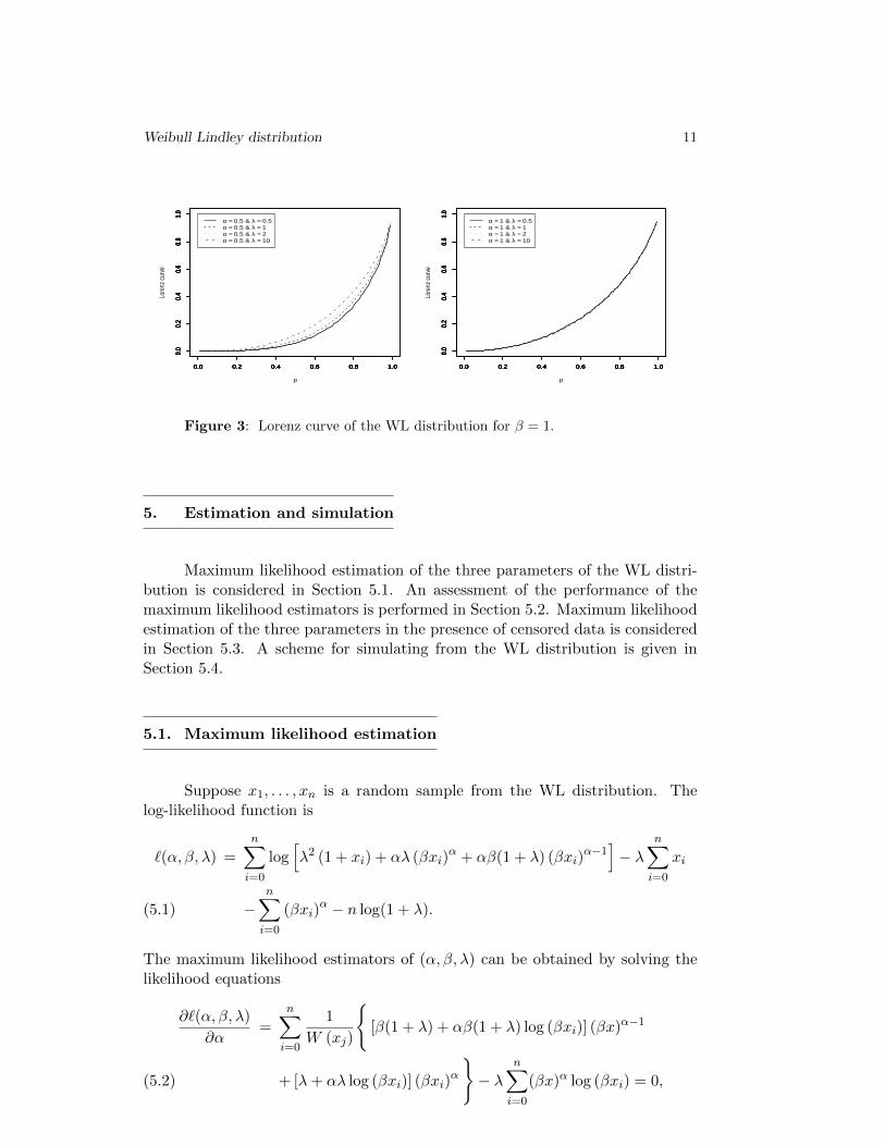
Possible shapes of (4.1) versus α and λ are shown in Figure 3. When α = 0.5, thecurves bend further towards the diagonal line as λ increases. When α = 1, thecurves bend further away from the diagonal line as λ increases. For each fixed λ,the curves bend further towards the diagonal line as α increases.


0.0 0.2 0.4 0.6 0.8 1.0

0.0

0.2

0.4

0.6

0.8

1.0

p

Lore

nz c

urve

0.0 0.2 0.4 0.6 0.8 1.0

0.0

0.2

0.4

0.6

0.8

1.0

0.0 0.2 0.4 0.6 0.8 1.0

0.0

0.2

0.4

0.6

0.8

1.0

0.0 0.2 0.4 0.6 0.8 1.0

0.0

0.2

0.4

0.6

0.8

1.0

0.0 0.2 0.4 0.6 0.8 1.0

0.0

0.2

0.4

0.6

0.8

1.0

α = 0.5 & λ = 0.5α = 0.5 & λ = 1α = 0.5 & λ = 2α = 0.5 & λ = 10

0.0 0.2 0.4 0.6 0.8 1.0

0.0

0.2

0.4

0.6

0.8

1.0

p

Lore

nz c

urve

0.0 0.2 0.4 0.6 0.8 1.0

0.0

0.2

0.4

0.6

0.8

1.0

0.0 0.2 0.4 0.6 0.8 1.0

0.0

0.2

0.4

0.6

0.8

1.0

0.0 0.2 0.4 0.6 0.8 1.0

0.0

0.2

0.4

0.6

0.8

1.0

0.0 0.2 0.4 0.6 0.8 1.0

0.0

0.2

0.4

0.6

0.8

1.0

α = 1 & λ = 0.5α = 1 & λ = 1α = 1 & λ = 2α = 1 & λ = 10

Figure 3: Lorenz curve of the WL distribution for β = 1.

5. Estimation and simulation

Maximum likelihood estimation of the three parameters of the WL distri-bution is considered in Section 5.1. An assessment of the performance of themaximum likelihood estimators is performed in Section 5.2. Maximum likelihoodestimation of the three parameters in the presence of censored data is consideredin Section 5.3. A scheme for simulating from the WL distribution is given inSection 5.4.

5.1. Maximum likelihood estimation

Suppose x1, . . . , xn is a random sample from the WL distribution. Thelog-likelihood function is

`(α, β, λ) =

n∑i=0

log[λ2 (1 + xi) + αλ (βxi)

α + αβ(1 + λ) (βxi)α−1]− λ

n∑i=0

xi

−n∑i=0

(βxi)α − n log(1 + λ).(5.1)

The maximum likelihood estimators of (α, β, λ) can be obtained by solving thelikelihood equations

∂`(α, β, λ)

∂α=

n∑i=0

1

W (xj)

{[β(1 + λ) + αβ(1 + λ) log (βxi)] (βx)α−1

+ [λ+ αλ log (βxi)] (βxi)α

}− λ

n∑i=0

(βx)α log (βxi) = 0,(5.2)


∂`(α, β, λ)

∂β=

n∑i=0

1

βW (xi)

[αβ (1 + xi) (βxi)

α−1 + α2λ (βxi)α]− α

β

n∑i=0

(βxi)α = 0(5.3)

and

∂`(α, β, λ)

∂λ=

n∑i=0

1

W (xi)

[α (βxi)

α + αβ (βxi)α−1 + 2λ (1 + xi)

]−

n∑i=0

xi −n

1 + λ= 0,(5.4)

where W (x) = λ2(1 + x) + αλ(βx)α + αβ(1 + λ)(βx)α−1. Alternatively, theMLEs can be obtained by maximizing (5.1) numerically. We shall use the latterapproach in Sections 5.2 and 6. The maximization was performed by using thenlm function in R (R Development Core Team [25]). In Sections 5.2 and 6, thefunction nlm was executed with the initial values taken to be:

i) the true parameter values (applicable for Section 5.2 only);

ii) α = 0.01, 0.02, . . . , 10, β = 0.01, 0.02, . . . , 10 and λ = 0.01, 0.02, . . . , 10;

iii) the moments estimates, i.e., the solutions E(X) = (1/n)

n∑i=1

xi, E(X2)

=

(1/n)n∑i=1

x2i and E(X3)

= (1/n)n∑i=1

x3i , where E(X), E(X2)

and E(X3)

are given by (3.2). These equations do not give explicit solutions. Theywere solved numerically using a quasi-Newton algorithm. Numerical inves-tigations showed that this involved roughly the same amount of time assolving of ∂`(α,β,λ)∂α = 0, ∂`(α,β,λ)∂β = 0 and ∂`(α,β,λ)

∂λ = 0 using a quasi-Newtonalgorithm.

In the cases of i) and iii), the function nlm converged all the time and the MLEswere unique. In the case of ii), the MLEs were unique whenever the function nlmconverged. In the case of ii), the function nlm did not converge about five percentof the time.

For interval estimation of (α, β, λ), we consider the observed Fisher infor-mation matrix given by

IF (α, β, λ) = −

Iαα Iαβ IαλIβα Iββ IβλIλα Iλβ Iλλ

,

where Iφ1φ2 = ∂2`/∂φ1∂φ2.

Under certain regularity conditions (see, for example, Ferguson [?]) andLehmann and Casella [19], pages 461-463) and for large n, the distribution of√n(α− α, β − β, λ− λ

)can be approximated by a trivariate normal distribu-

tion with zero means and variance-covariance matrix given by the inverse ofthe observed information matrix evaluated at the maximum likelihood estimates.


This approximation can be used to construct approximate confidence intervals,confidence regions, and testing hypotheses for the parameters. For example,

an asymptotic confidence interval for α with level 1 − γ is(α∓ z1−γ/2

√I α,α

),

where I α,α is the (1, 1)th element of the inverse of IF

(α, β, λ

)and z1−γ/2 is the

(1− γ/2)th quartile of the standard normal distribution.

5.2. Simulation study

Here, we assess the performance of the maximum likelihood estimatorsgiven by (5.2)-(5.4) with respect to sample size n. The assessment was based ona simulation study:

1. generate ten thousand samples of size n from (1.2). The inversion methodwas used to generate samples, i.e., variates of the WL distribution weregenerated using

U =1 + λ

λ

[(1− p)eλX+(βX)α − 1

],

where U ∼ U(0, 1) is a uniform variate on the unit interval.

2. compute the maximum likelihood estimates for the ten thousand samples,

say(αi, βi, λi

)for i = 1, 2, . . . , 10000.

3. compute the biases and mean squared errors given by

biash(n) =1

10000

10000∑i=1

(hi − h

), MSEh(n) =

1

10000

10000∑i=1

(hi − h

)2for h = α, β, λ.

We repeated these steps for n = 10, 11, . . . , 100 with α = 1, β = 1 and λ = 1, socomputing biash(n) and MSEh(n) for h = α, β, λ and n = 10, 11, . . . , 100.


20 40 60 80 100

−0.

035

−0.

020

−0.

005

n

Bia

s of

MLE

(al

pha)

20 40 60 80 100

−0.

008

−0.

004

n

Bia

s of

MLE

(be

ta)

20 40 60 80 100

−0.

008

−0.

004

n

Bia

s of

MLE

(la

mbd

a)

Figure 4: Biases of(α, β, λ

)versus n.


20 40 60 80 100

0.02

0.03

0.04

0.05

n

MS

E o

f MLE

(al

pha)

20 40 60 80 100

0.01

00.

014

0.01

8

n

MS

E o

f MLE

(be

ta)

20 40 60 80 100

0.00

780.

0084

n

MS

E o

f MLE

(la

mbd

a)

Figure 5: Mean squared errors of(α, β, λ

)versus n.

Figures 4 and 5 show how the three biases and the three mean squared errorsvary with respect to n. The following observations can be made: the biases foreach parameter are negative; the biases appear largest for the parameter, α; thebiases appear smallest for the parameters, β and λ; the biases for each parameterincrease to zero as n→∞; the mean squared errors for each parameter decrease tozero as n→∞; the mean squared errors appear largest for the parameter, α; themean squared errors appear smallest for the parameter, λ. These observationsare for only one choice for (α, β, λ), namely that (α, β, λ) = (1, 1, 1). But theresults were similar for a wide range of other values of (α, β, λ). In particular,the biases for each parameter always increased to zero as n → ∞ and the meansquared errors for each parameter always decreased to zero as n→∞.

Section 6 presents three real data applications. The sample size for thefirst data set is eight hundred and seventy seven. The sample size for the seconddata set is twenty six. The sample size for the third data set is two hundred andninety five. We shall see later in Section 6 that the WL distribution providesgood fits to the three data sets. Based on this fact, the biases for α, β and λ canbe expected to be less than 0.025, 0.007 and 0.0075, respectively, for all of thedata sets. The mean squared errors for α, β and λ can be expected to be lessthan 0.04, 0.02 and 0.0088, respectively, for all of the data sets. Hence, the point


estimates given in Section 6 for all data sets can be considered accurate enough.

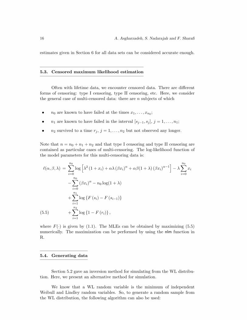
5.3. Censored maximum likelihood estimation

Often with lifetime data, we encounter censored data. There are differentforms of censoring: type I censoring, type II censoring, etc. Here, we considerthe general case of multi-censored data: there are n subjects of which

• n0 are known to have failed at the times x1, . . . , xn0 ;

• n1 are known to have failed in the interval [sj−1, sj ], j = 1, . . . , n1;

• n2 survived to a time rj , j = 1, . . . , n2 but not observed any longer.

Note that n = n0 + n1 + n2 and that type I censoring and type II censoring arecontained as particular cases of multi-censoring. The log-likelihood function ofthe model parameters for this multi-censoring data is:

`(α, β, λ) =

n0∑i=0

log[λ2 (1 + xi) + αλ (βxi)

α + αβ(1 + λ) (βxi)α−1]− λ

n0∑i=0

xi

−n0∑i=0

(βxi)α − n0 log(1 + λ)

+

n1∑i=1

log {F (si)− F (si−1)}

+

n2∑i=1

log {1− F (ri)} ,(5.5)

where F (·) is given by (1.1). The MLEs can be obtained by maximizing (5.5)numerically. The maximization can be performed by using the nlm function inR.

5.4. Generating data

Section 5.2 gave an inversion method for simulating from the WL distribu-tion. Here, we present an alternative method for simulation.

We know that a WL random variable is the minimum of independentWeibull and Lindley random variables. So, to generate a random sample fromthe WL distribution, the following algorithm can also be used:


1. First generate a random sample v1, . . . , vn from Weibull(α, β);2. Independently, generate a random sample w1, . . . , wn from Lindley(λ);3. Set xi = min (vi, wi) for i = 1, . . . , n.

Then x1, x2, . . . , xn will be a random sample from WL(α, β, λ).

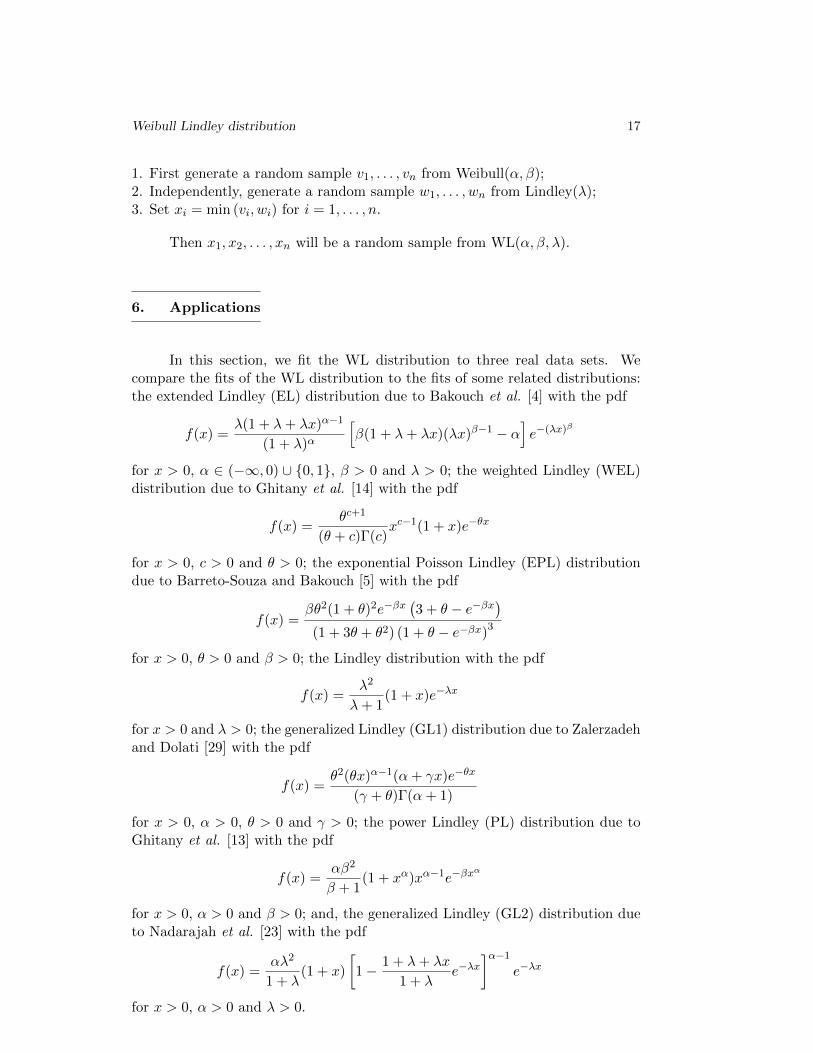
6. Applications

In this section, we fit the WL distribution to three real data sets. Wecompare the fits of the WL distribution to the fits of some related distributions:the extended Lindley (EL) distribution due to Bakouch et al. [4] with the pdf

f(x) =λ(1 + λ+ λx)α−1

(1 + λ)α

[β(1 + λ+ λx)(λx)β−1 − α

]e−(λx)

β

for x > 0, α ∈ (−∞, 0) ∪ {0, 1}, β > 0 and λ > 0; the weighted Lindley (WEL)distribution due to Ghitany et al. [14] with the pdf

f(x) =θc+1

(θ + c)Γ(c)xc−1(1 + x)e−θx

for x > 0, c > 0 and θ > 0; the exponential Poisson Lindley (EPL) distributiondue to Barreto-Souza and Bakouch [5] with the pdf

f(x) =βθ2(1 + θ)2e−βx

(3 + θ − e−βx

)(1 + 3θ + θ2) (1 + θ − e−βx)

3

for x > 0, θ > 0 and β > 0; the Lindley distribution with the pdf

f(x) =λ2

λ+ 1(1 + x)e−λx

for x > 0 and λ > 0; the generalized Lindley (GL1) distribution due to Zalerzadehand Dolati [29] with the pdf

f(x) =θ2(θx)α−1(α+ γx)e−θx

(γ + θ)Γ(α+ 1)

for x > 0, α > 0, θ > 0 and γ > 0; the power Lindley (PL) distribution due toGhitany et al. [13] with the pdf

f(x) =αβ2

β + 1(1 + xα)xα−1e−βx

α

for x > 0, α > 0 and β > 0; and, the generalized Lindley (GL2) distribution dueto Nadarajah et al. [23] with the pdf

f(x) =αλ2

1 + λ(1 + x)

[1− 1 + λ+ λx

1 + λe−λx

]α−1e−λx

for x > 0, α > 0 and λ > 0.


6.1. Data set 1

The first data are times to reinfection of STD for eight hundred and seventyseven patients. The data were taken from Section 1.12 of Klein and Moeschberger[17]. We fitted the eight distributions to the data. Table 1 gives the parameterestimates, standard errors obtained by inverting the observed information ma-trix, log-likelihood values, values of Akaike information criterion (AIC), values ofBayesian information criterion (BIC), p values based on the Kolmogorov-Smirnov(KS) statistic, p values based on the Anderson Darling (AD) statistic, and p val-ues based on the Cramer-von Mises (CVM) statistic. The fitted pdfs of the threebest fitting distributions as well as the empirical histogram are shown in Figure6. The corresponding probability plots are shown in Figure 7.

We can see that the WL distribution gives the smallest AIC value, thesmallest BIC value, the largest p value based on the KS statistic, the largestp value based on the AD statistic, and the largest p value based on the CVMstatistic. The second smallest AIC, BIC values and the second largest p values aregiven by the GL2 distribution. The third smallest AIC, BIC values and the thirdlargest p values are given by the EPL distribution. The fourth smallest AIC, BICvalues and the fourth largest p values are given by the PL distribution. The fifthsmallest AIC, BIC values and the fifth largest p values are given by the WELdistribution. The sixth smallest AIC, BIC values and the sixth largest p valuesare given by the Lindley distribution. The seventh smallest AIC, BIC values andthe seventh largest p values are given by the EL distribution. The largest AIC,BIC values and the smallest p values are given by the GL1 distribution.

Hence, the WL distribution provides the best fit based on the AIC values,BIC values, p values based on the KS statistic, p values based on the AD statistic,and p values based on the CVM statistic. The density and probability plots alsoshow that the WL distribution provides the best fit.


Distribution Parameter estimates (s.e) − logL AIC BIC KS AD CVM

EL λ = 8.806 × 10−1(1.302 × 10−2

), 9203.4 18412.9 18427.2 4.080 × 10−4 2.700 × 10−5 1.979 × 10−4

α = −9.804 × 10−1(3.034 × 10−2

),

β = 9.935 × 10−7(8.098 × 10−3

)WEL θ = 2.878 × 10−3

(1.076 × 10−4

), 6082.4 12168.7 12178.3 9.474 × 10−3 2.879 × 10−4 6.021 × 10−2

c = 9.359 × 10−2(1.324 × 10−2

)EPL θ = 2.326

(7.568 × 10−1

), 6055.1 12114.1 12123.7 8.151 × 10−2 1.395 × 10−2 1.174 × 10−1

β = 2.190 × 10−3(1.854 × 10−4

)Lindley λ = 5.397 × 10−3

(1.313 × 10−4

)6413.0 12828.1 12832.9 1.996 × 10−3 1.762 × 10−4 5.579 × 10−4

GL1 θ = 7.872 × 10−2(4.339 × 10−3

), 27827.1 55660.1 55674.4 1.864 × 10−5 2.149 × 10−5 1.697 × 10−4

α = 1.453 × 10−6(4.164 × 10−2

),

γ = 7.595 × 10−1(6.225 × 10−2

)PL α = 5.696 × 10−1

(1.364 × 10−2

), 6056.3 12116.7 12126.2 6.872 × 10−2 1.232 × 10−3 7.611 × 10−2

β = 7.671 × 10−2(6.420 × 10−3

)GL2 λ = 2.980 × 10−3

(1.391 × 10−4

), 6031.8 12067.5 12077.1 1.695 × 10−1 7.568 × 10−2 1.480 × 10−1

α = 3.660 × 10−1(1.509 × 10−2

)WL λ = 2.331 × 10−3

(2.714 × 10−4

), 6022.9 12051.7 12066.0 3.131 × 10−1 8.243 × 10−2 2.735 × 10−1

α = 6.435 × 10−1(3.870 × 10−2

),

β = 1.740 × 10−3(2.792 × 10−4

)

Table 1: Parameter estimates, standard errors, log-likelihoods, AICs,BICs and goodness-of-fit measures for data set 1.


Data

Fitte

d PD

Fs

0 500 1000 1500

0.00

00.

001

0.00

20.

003

0.00

4

0 500 1000 1500

0.00

00.

001

0.00

20.

003

0.00

4

0 500 1000 1500

0.00

00.

001

0.00

20.

003

0.00

4

0 500 1000 1500

0.00

00.

001

0.00

20.

003

0.00

4

EPLGL2WL

Figure 6: Fitted pdfs of the three best fitting distributions for data set 1.


0.0 0.2 0.4 0.6 0.8 1.0

0.0

0.2

0.4

0.6

0.8

1.0

Expected

Ob

se

rve

d

0.0 0.2 0.4 0.6 0.8 1.0

0.0

0.2

0.4

0.6

0.8

1.0

Expected

Ob

se

rve

d

0.0 0.2 0.4 0.6 0.8 1.0

0.0

0.2

0.4

0.6

0.8

1.0

Expected

Ob

se

rve

d

Figure 7: PP plots of the three best fitting distributions for data set 1(yellow for the EPL distribution, red for the GL2 distributionand black for the WL distribution).


6.2. Data set 2

The second data are times to death of twenty six psychiatric patients. Thedata were taken from Section 1.15 of Klein and Moeschberger [17]. The eightdistributions were fitted to this data. The parameter estimates, standard errorsand the various measures are given in Table 2. The corresponding density andprobability plots are shown in Figures 8 and 9, respectively.

We can see again that the WL distribution gives the smallest AIC value,the smallest BIC value, the largest p value based on the KS statistic, the largestp value based on the AD statistic, and the largest p value based on the CVMstatistic. The second smallest AIC, BIC values and the second largest p valuesare given by the Lindley distribution. The third smallest AIC, BIC values and thethird largest p values are given by the PL distribution. The fourth smallest AIC,BIC values and the fourth largest p values are given by the WEL distribution.The fifth smallest AIC, BIC values and the fifth largest p values are given by theGL2 distribution. The sixth smallest AIC, BIC values and the sixth largest pvalues are given by the GL1 distribution. The seventh smallest AIC, BIC valuesand the seventh largest p values are given by the EPL distribution. The largestAIC, BIC values and the smallest p values are given by the EL distribution.

Hence, the WL distribution again provides the best fit based on the AICvalues, BIC values, p values based on the KS statistic, p values based on the ADstatistic, and p values based on the CVM statistic. The density and probabilityplots again show that the WL distribution provides the best fit.



EL λ = 7.510 × 10−1(9.604 × 10−2

), 164.9 335.8 339.5 1.163 × 10−3 3.780 × 10−5 9.083 × 10−5

α = −8.534 × 10−1(2.414 × 10−1

),

β = 2.050 × 10−6(1.197 × 10−1

)WEL θ = 7.727 × 10−2

(2.090 × 10−2

), 107.7 219.3 221.8 4.691 × 10−1 1.392 × 10−3 3.064 × 10−2

c = 1.107(4.659 × 10−1

)EPL θ = 1.267 × 104

(4.662 × 105

), 111.1 226.3 228.8 1.840 × 10−2 4.964 × 10−5 1.024 × 10−4

β = 3.784 × 10−2(7.442 × 10−3

)Lindley λ = 7.311 × 10−2

(1.016 × 10−2

)107.7 217.4 218.6 7.924 × 10−1 1.126 × 10−2 4.895 × 10−2

GL1 θ = 8.282 × 10−2(2.152 × 10−2

), 107.1 220.3 224.0 2.920 × 10−2 1.163 × 10−4 7.787 × 10−4

α = 1.420(5.569 × 10−1

),

γ = 2.742 × 10−1(3.199 × 10−1

)PL α = 1.225

(2.069 × 10−1

), 106.9 217.8 220.3 6.957 × 10−1 8.737 × 10−3 3.715 × 10−2

β = 3.452 × 10−2(2.470 × 10−2

)GL2 λ = 7.547 × 10−2

(1.398 × 10−2

), 107.7 219.3 221.8 1.081 × 10−1 1.582 × 10−4 4.384 × 10−3

α = 1.069(2.874 × 10−1

)WL λ = 4.340 × 10−2

(1.051 × 10−2

), 93.4 192.8 196.5 8.998 × 10−1 8.372 × 10−1 2.849 × 10−1

α = 9.901 (2.822),

β = 2.832 × 10−2(1.014 × 10−3

)


Data

Fitte

d PD

Fs

0 10 20 30 40

0.00

0.02

0.04

0.06

0.08

0 10 20 30 40

0.00

0.02

0.04

0.06

0.08

0 10 20 30 40

0.00

0.02

0.04

0.06

0.08

0 10 20 30 40

0.00

0.02

0.04

0.06

0.08

LindleyPLWL



0.0 0.2 0.4 0.6 0.8 1.0

0.0

0.2

0.4

0.6

0.8

1.0

Expected

Ob

se

rve

d

0.0 0.2 0.4 0.6 0.8 1.0

0.0

0.2

0.4

0.6

0.8

1.0

Expected

Ob

se

rve

d

0.0 0.2 0.4 0.6 0.8 1.0

0.0

0.2

0.4

0.6

0.8

1.0

Expected

Ob

se

rve

d

Figure 9: PP plots of the three best fitting distributions for data set 2(brown for the Lindley distribution, blue for the PL distributionand black for the WL distribution).


6.3. Data set 3

The third data are times to infection for AIDS for two hundred and ninetyfive patients. The data were taken from Section 1.19 of Klein and Moeschberger[17]. The eight distributions were fitted to this data. The parameter estimates,standard errors and the various measures are given in Table 3. The correspondingdensity and probability plots are shown in Figures 10 and 11, respectively.

We can see yet again that the WL distribution gives the smallest AIC value,the smallest BIC value, the largest p value based on the KS statistic, the largestp value based on the AD statistic, and the largest p value based on the CVMstatistic. The second smallest AIC, BIC values and the second largest p valuesare given by the EL distribution. The third smallest AIC, BIC values and thethird largest p values are given by the PL distribution. The fourth smallest AIC,BIC values and the fourth largest p values are given by the WEL distribution.The fifth smallest AIC, BIC values and the fifth largest p values are given by theGL1 distribution. The sixth smallest AIC, BIC values and the sixth largest pvalues are given by the GL2 distribution. The seventh smallest AIC, BIC valuesand the seventh largest p values are given by the Lindley distribution. The largestAIC, BIC values and the smallest p values are given by the EPL distribution.

Hence, the WL distribution yet again provides the best fit based on theAIC values, BIC values, p values based on the KS statistic, p values based onthe AD statistic, and p values based on the CVM statistic. The density andprobability plots yet again show that the WL distribution provides the best fit.



EL λ = 2.066 × 10−1(5.340 × 10−3

), 537.5 1080.9 1092.0 7.775 × 10−1 9.719 × 10−1 1.866 × 10−1

α = −1.425 × 10−1(8.097 × 10−2

),

β = 3.503(2.776 × 10−1

)WEL θ = 1.396

(1.130 × 10−1

), 563.3 1130.6 1138.0 2.072 × 10−1 1.269 × 10−1 9.133 × 10−3

c = 5.025(4.472 × 10−1

)EPL θ = 1.145 × 104

(1.091 × 105

), 713.2 1430.4 1437.8 6.394 × 10−2 2.022 × 10−2 7.102 × 10−4

β = 2.403 × 10−1(1.402 × 10−2

)Lindley λ = 4.106 × 10−1

(1.731 × 10−2

)659.7 1321.4 1325.1 1.113 × 10−1 8.193 × 10−2 1.443 × 10−3

GL1 θ = 1.402(1.157 × 10−1

), 563.3 1132.5 1143.6 1.744 × 10−1 9.239 × 10−2 3.008 × 10−3

α = 5.099(5.533 × 10−1

),

γ = 3.872 (4.373)

PL α = 2.099(8.683 × 10−2

), 544.7 1093.5 1100.9 5.437 × 10−1 1.664 × 10−1 3.248 × 10−2

β = 8.357 × 10−2(1.176 × 10−2

)GL2 λ = 7.544 × 10−1

(3.321 × 10−2

), 571.4 1146.9 1154.2 1.136 × 10−1 9.136 × 10−2 1.616 × 10−3

α = 4.536(4.812 × 10−1

)WL λ = 1.595 × 10−1

(3.235 × 10−2

), 535.7 1077.4 1088.4 8.059 × 10−1 9.908 × 10−1 8.666 × 10−1

α = 4.036(4.329 × 10−1

),

β = 1.949 × 10−1(6.412 × 10−3

)


Data

Fitte

d PD

Fs

0 2 4 6

0.00

0.05

0.10

0.15

0.20

0.25

0.30

0 2 4 6

0.00

0.05

0.10

0.15

0.20

0.25

0.30

0 2 4 6

0.00

0.05

0.10

0.15

0.20

0.25

0.30

0 2 4 6

0.00

0.05

0.10

0.15

0.20

0.25

0.30

ELPLWL



0.0 0.2 0.4 0.6 0.8 1.0

0.0

0.2

0.4

0.6

0.8

1.0

Expected

Ob

se

rve

d

0.0 0.2 0.4 0.6 0.8 1.0

0.0

0.2

0.4

0.6

0.8

1.0

Expected

Ob

se

rve

d

0.0 0.2 0.4 0.6 0.8 1.0

0.0

0.2

0.4

0.6

0.8

1.0

Expected

Ob

se

rve

d

Figure 11: PP plots of the three best fitting distributions for data set 3(pink for the EL distribution, blue for the PL distribution andblack for the WL distribution).


7. Conclusions

We have introduced a three-parameter generalization of the Lindley distri-bution referred to as the Weibull Lindley distribution. We have provided at leastseven possible motivations for this new distribution. We have studied shapesof probability density and hazard rate functions, moments, moment generatingfunction, Lorenz curve, maximum likelihood estimators in the presence of com-plete data and maximum likelihood estimators in the presence of censored data.We have assessed the finite sample performance of the maximum likelihood esti-mators by simulation. We have provided three real data applications.

We have seen that the probability density function can be bimodal, uni-modal, monotonically decreasing or monotonically decreasing with an inflexionpoint. The hazard rate function can be monotonically increasing, monotonicallydecreasing or bathtub shaped. The maximum likelihood estimators appear to beregular for sample sizes larger than twenty. The data applications show that theWeibull Lindley distribution provides better fits than all known generalizationsof the Lindley distribution for at least three data sets.

ACKNOWLEDGMENTS

The authors would like to thank the Editor, the Associate Editor and thereferee for careful reading and comments which greatly improved the paper.

REFERENCES

[1] Adamidis, K. and Loukas, S. (1998). A lifetime distribution with decreasingfailure rate. Statistics and Probability Letters, 39, 35-42.

[2] Andersen, P. K. and Skrondal, A. (2015). A competing risks approach to“biologic” interaction. Lifetime Data Analysis, 21, 300-314.

[3] Asgharzadeh, A., Bakouch, H.S. and Esmaeili, L. (2013). Pareto Poisson-Lindley distribution with applications. Journal of Applied Statistics, 40, 1717-1734.

[4] Bakouch, H.S., Al-Zahrani, B.M., Al-Shomrani, A.A., Marchi,V.A.A. and Louzada, F. (2012). An extended Lindley distribution. Journalof the Korean Statistical Society, 41, 75-85.

[5] Barreto-Souza, W. and Bakouch, H.S. (2013). A new lifetime model withdecreasing failure rate. Statistics, 47, 465-476.


[6] Barreto-Souza, W., Morais, A.L. and Cordeiro, G.M. (2011). TheWeibull-geometric distribution. Journal of Statistical Computation and Simu-lation, 81, 645-657.

[7] Bourguignon, M., Silva, R.B. and Cordeiro, G.M. (2014). A new classof fatigue life distributions. Journal of Statistical Computation and Simulation,84, 2619-2635.

[8] Cadarso-Suarez, C., Meira-Machado, L., Kneib, T. and Gude, F.(2010). Flexible hazard ratio curves for continuous predictors in multi-state mod-els: An application to breast cancer data. Statistical Modelling, 10, 291-314.

[9] Egghe, L. (2002). Development of hierarchy theory for digraphs using concen-tration theory based on a new type of Lorenz curve. Mathematical and ComputerModelling, 36, 587-602.

[10] Ferguson, T.S. (1996). A Course in Large Sample Theory. Chapman and Hall,London.

[11] Gail, M.H. (2009). Applying the Lorenz curve to disease risk to optimize healthbenefits under cost constraints. Statistics and Its Interface, 2, 117-121.

[12] Gail, M.H. and Benichou, J. (2000). Encyclopedia of Epidemiologic Methods.John Wiley and Sons.

[13] Ghitany, M.E., Al-Mutairi, D.K., Balakrishnan, N. and Al-Enezi,L.J. (2013). Power Lindley distribution and associated inference. ComputationalStatistics and Data Analysis, 64, 20-33.

[14] Ghitany, M.E., Alqallaf, F., Al-Mutairi, D.K. and Husain, H.A.(2011). A two-parameter weighted Lindley distribution and its applications tosurvival data. Mathematics and Computers in Simulation, 81, 1190-1201.

[15] Ghitany, M.E., Atieh, B. and Nadarajah, S. (2008). Lindley distributionand its application. Mathematics and Computers in Simulation, 78, 493-506.

[16] Groves-Kirkby, C.J., Denman, A.R. and Phillips, P.S. (2009). Lorenzcurve and Gini coefficient: Novel tools for analysing seasonal variation of envi-ronmental radon gas. Journal of Environmental Management, 90, 2480-2487.

[17] Klein, J.P. and Moeschberger, M.L. (1997). Survival Analysis Techniquesfor Censored and Truncated Data. Springer Verlag, New York.

[18] Kus, C. (2007). A new lifetime distribution. Computational Statistics and DataAnalysis, 51, 4497-4509.

[19] Lehmann, L.E. and Casella, G. (1998). Theory of Point Estimation, secondedition. Springer Verlag, New York.

[20] Lindley, D.V. (1958). Fiducial distributions and Bayes’ theorem. Journal ofthe Royal Statistical Society, A, 20, 102-107.

[21] Maldonado, A., Perez-Ocon, R. and Herrera, A. (2007). Depression andcognition: New insights from the Lorenz curve and the Gini index. InternationalJournal of Clinical and Health Psychology, 7, 21-39.

[22] Morais, A.L. and Barreto-Souza, W. (2011). A compound class of Weibulland power series distributions. Computational Statistics and Data Analysis, 55,1410-1425.

[23] Nadarajah, S., Bakouch, H.S. and Tahmasbi, R. (2011). A generalizedLindley distribution. Sankhya, B, 73, 331-359.


[24] Nair, U. N., Sankaran, P. G. and Balakrishnan, N. (2010). Quantile-Based Reliability Analysis. Birkhauser, Boston.

[25] R Development Core Team (2014). A Language and Environment for Sta-tistical Computing. R Foundation for Statistical Computing. Vienna, Austria.

[26] Radice, A. (2009). Use of the Lorenz curve to quantify statistical nonuniformityof sediment transport rate. Journal of Hydraulic Engineering, 135, 320-326.

[27] Silva, R.B., Bourguignon, M., Dias, C.R.B. and Cordeiro, G.M. (2013).The compound class of extended Weibull power series distributions. Computa-tional Statistics and Data Analysis, 58, 352-367.

[28] Yamaguchi, K. (1993). Modeling time-varying effects of covariates in event-history analysis using statistics from the saturated hazard rate model. Sociolog-ical Methodology, 23, 279-317.

[29] Zakerzadeh, H. and Dolati, A. (2009). Generalized Lindley distribution.Journal of Mathematical Extension, 3, 13-25.

weibull lindley distribution - statistics portugal · weibull lindley distribution authors: a....

Documents