weight of evidence checklist review aoh work group call june 7, 2006 joe adlhoch - air resource...
Post on 20-Dec-2015
214 views
TRANSCRIPT

Weight of Evidence Checklist Review
AoH Work Group CallJune 7, 2006Joe Adlhoch - Air Resource Specialists, Inc.

Class I Area Profile → WOE Checklist
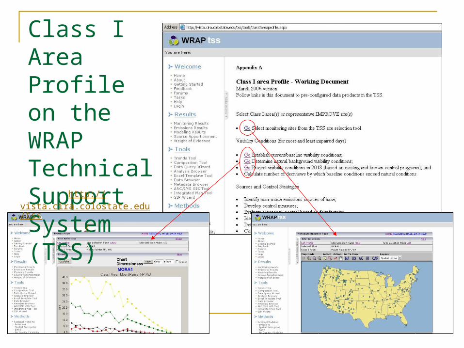
Class I Area Profile on the WRAP Technical Support System (TSS)
http://vista.cira.colostate.edu/tss/

Draft WOE Checklist (Step 1)
Summary of available information General Class I area information (location, size,
topography, discussion of importance, etc.) Overview summary of basic data sets:
Visibility monitoring Emission inventories Modeling results
Will vary according to state (e.g., no CMAQ modeling done for AK; some states have international borders)
Style will be customized by each state
Draft WOE Checklist (Step 2)
Analysis of visibility conditions What are current (baseline, 2000-04) visibility
conditions? What is the relative importance of each species?
What does the RHR glide path look like? What are estimated natural visibility conditions? What does the model predict for 2018?

Baseline Conditions at Sawtooth, ID
20% Worst Vis. Days Species Contribution Sulfate Medium Nitrate Low Organics High EC Medium CM Low Soil Low

Uniform Rate of Reasonable Progress Glide PathSawtooth Wilderness - 20% Worst Days
12.5 12.111.2
10.39.5
8.67.7
7.2
12.7
0
5
10
15
20
2000 2004 2008 2012 2016 2020 2024 2028 2032 2036 2040 2044 2048 2052 2056 2060 2064
Year
Ha
zin
ess
In
de
x (D
eci
vie
ws)
Glide Path Natural Condition (Worst Days) Observation Method 1 Prediction
Regional Haze Rule Glide Path for Sawtooth
Model results for the 2018 base case do not predict Sawtooth’s visibility (in terms of deciview) will be on or below the glide path
Draft WOE Checklist (Step 3)
Analysis of visibility conditions by individual species What do individual species glide paths (measured in
extinction) look like? Need to define natural conditions appropriately (following
examples assume “annual average” natural conditions, not 20% worst)
Which species show predicted 2018 values at or below the glide path?
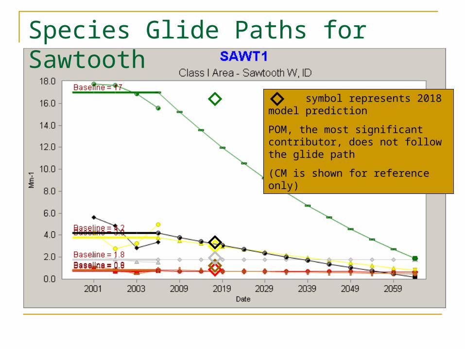
Species Glide Paths for Sawtooth
symbol represents 2018 model prediction
POM, the most significant contributor, does not follow the glide path
(CM is shown for reference only)

Draft WOE Checklist (Step 4)
Review monitoring uncertainties and model performance for each species What level of monitoring uncertainties are associated
with each species? Lab uncertainties (can be calculated from IMPROVE data set Other uncertainties (flow rate problems, clogged filters) may
be difficult to quantify How well does the model predict the monitoring data?
Good model performance is most important for highest contributing species
What does performance look like seasonally and over all?

IMPROVE (top) vs. Model (bottom)
Seasonal variations in major species is reasonably similar

Worst 20% Obs (left) vs Plan02b (right) at SAWT1
0
5
10
15
20
25
30
35
40
45
50
116 137 140 170 179 191 194 197 200 203 206 212 215 218 224 230 233 254 269 296 299 317 _ _ _ Avg
Julian Day in Worst 20% group
bE
XT
(1/
Mm
)
bCM
bSOIL
bEC
bOC
bNO3
bSO4
2002 Model Performance, Worst Days
Carbon somewhat low but reasonable
Sulfate, nitrate and soil similar
CM shows very poor performance
Draft WOE Checklist (Step 5)
Integrate information about each species: monitoring, modeling, and emissions data Do changes in emissions agree with model
predictions for 2018? How do we know what source region of emissions to
compare? Weight emissions by back trajectory residence times to
estimate what emissions have the potential to impact a given Class I area
Do weighted emissions described above support attribution results derived from PSAT and PMF?

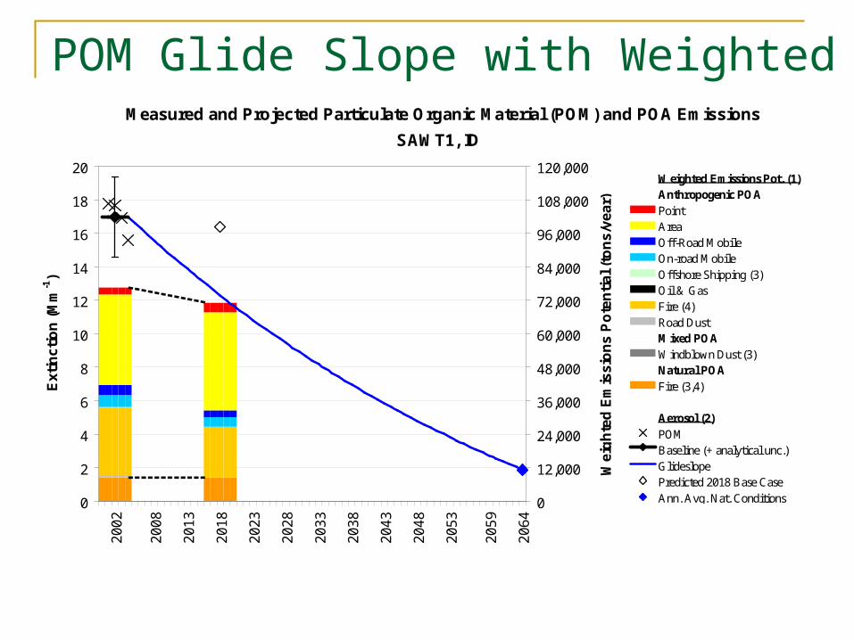
POM Glide Slope with Weighted EmissionsMeasured and Projected Particulate Organic Material (POM) and POA Emissions
SAWT1, ID
0
2
4
6
8
10
12
14
16
18
20
20
02
20
08
20
13
20
18
20
23
20
28
20
33
20
38
20
43
20
48
20
53
20
59
20
64
Ex
tin
ctio
n (
Mm
-1)
0
12,000
24,000
36,000
48,000
60,000
72,000
84,000
96,000
108,000
120,000
We
igh
ted
Em
issi
on
s P
ote
nti
al
(to
ns
/ye
ar)
Weighted Emissions Pot. (1)Anthropogenic POAPointAreaOff-Road MobileOn-road MobileOffshore Shipping (3)Oil & GasFire (4)Road DustMixed POAWindblown Dust (3)Natural POAFire (3,4)
Aerosol (2)POMBaseline (+ analytical unc.)GlideslopePredicted 2018 Base CaseAnn. Avg. Nat. Conditions
(1) Weighted Emissions Potential based on annual average emissions and back trajectory residence times for the 20% worst visibility days(2) Measured aerosol based on the 20% worst visibility days(3) Offshore shipping, natural fire, and windblown dust emissions were held constant for the 2018 base case(4) Fire emissions in the plan02 EI represent the entire 5 year baseline period
Baseline Extinction with Lab Uncertainty
Predicted 2018 Extinction
Weighted Emissions
POM Glide Slope with Weighted EmissionsMeasured and Projected Particulate Organic Material (POM) and POA Emissions
SAWT1, ID
0
2
4
6
8
10
12
14
16
18
20
20
02
20
08
20
13
20
18
20
23
20
28
20
33
20
38
20
43
20
48
20
53
20
59
20
64
Ex
tin
ctio
n (
Mm
-1)
0
12,000
24,000
36,000
48,000
60,000
72,000
84,000
96,000
108,000
120,000
We
igh
ted
Em
issi
on
s P
ote
nti
al
(to
ns
/ye
ar)
Weighted Emissions Pot. (1)Anthropogenic POAPointAreaOff-Road MobileOn-road MobileOffshore Shipping (3)Oil & GasFire (4)Road DustMixed POAWindblown Dust (3)Natural POAFire (3,4)
Aerosol (2)POMBaseline (+ analytical unc.)GlideslopePredicted 2018 Base CaseAnn. Avg. Nat. Conditions
(1) Weighted Emissions Potential based on annual average emissions and back trajectory residence times for the 20% worst visibility days(2) Measured aerosol based on the 20% worst visibility days(3) Offshore shipping, natural fire, and windblown dust emissions were held constant for the 2018 base case(4) Fire emissions in the plan02 EI represent the entire 5 year baseline period

Calculating Weighted Emissions Potential for a Class I Area
X =
Emissions Residence Times Weighted Emissions Potential
Use annual average emissions Use residence times based on 3 – 5 years of 8-day back trajectories
(20% worst days or all days) Weight the residence times by 1/distance from Class I area
(approximates dispersion and deposition) Very low residence time values have been ignored Results do not take into account chemical reactions (or biogenic VOC
emissions for secondary particulate formation)

Sawtooth: Primary Organic Aerosol
Total POA emissions X residence time = weighted emissions potential
Weighted emissions potential represents most probable source region emissions which contribute to POM at the selected monitoring site.

Estimating Relative Impacts of Emissions Source Regions The goal is to give states a tool to investigate
emissions source regions likely to impact their Class I areas
Review weighted emissionsby source region (states)Review total emissionswithin 2, 4, and 8 grid cellsof the site
Ultimately compare results with PSAT and/or PMF analyses
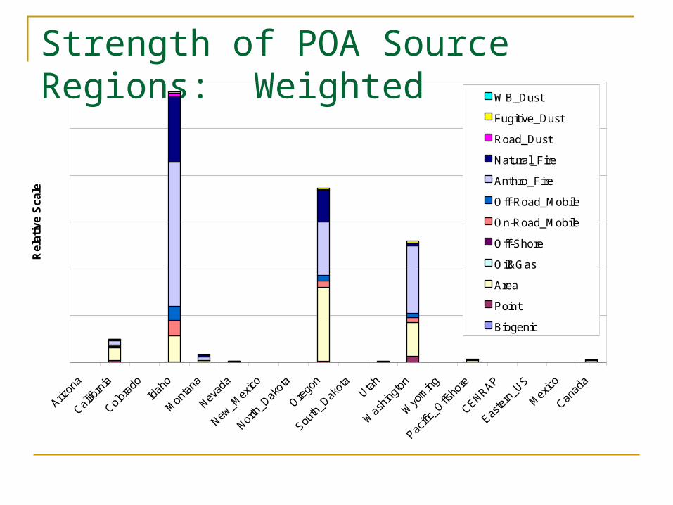
Strength of POA Source Regions: Weighted
Arizon
a
Califo
rnia
Colora
doId
aho
Mon
tana
Nevad
a
New_M
exico
North
_Dak
ota
Orego
n
South
_Dak
ota
Utah
Was
hingt
on
Wyo
ming
Pacific
_Offs
hore
CENRAP
Easte
rn_U
S
Mex
ico
Canad
a
Re
lati
ve
Sc
ale
WB_Dust
Fugitive_Dust
Road_Dust
Natural_Fire
Anthro_Fire
Off-Road_Mobile
On-Road_Mobile
Off-Shore
Oil&Gas
Area
Point
Biogenic
Draft WOE Checklist (Step 6)
Investigate specific questions that arise in steps 2 – 6 Review historical trends (if sufficient data exists) Review distributions of IMPROVE mass, and expected changes
predicted by the model Review natural, episodic events for their potential impact Do the results so far make sense? If not, deeper investigation
of data sets may be required Are there reasonable explanations for species that show and
don’t show progress along the glide path? Consider the other factors mandated by the RHR to determine
reasonable progress

Draft WOE Checklist (Step 7)
Repeat steps 2 – 6 with emissions and model results from various control strategies How do specific control strategies affect the outcome?

Draft WOE Checklist (Step 8)
Review available attribution information and determine which states need to consult about which Class I areas PSAT will be available for sulfate and nitrate (and
possible some portion of organics) PMF will be available for all species (?), but may be
used primarily for carbon and dust Emissions weighted by residence times will be
available for all species (pending certain sensitivity tests and caveats)