what is the future of slope stability analysis? is the future of slope stability analysis? (are we...
TRANSCRIPT

What is the Future of Slope What is the Future of Slope Stability Analysis?Stability Analysis?
(Are We Approaching the Limits of (Are We Approaching the Limits of Limit Equilibrium Analyses?)Limit Equilibrium Analyses?)
Dr. Delwyn G. FredlundDr. Delwyn G. FredlundUnsaturated Soil Technologies Ltd.Unsaturated Soil Technologies Ltd.
1714 East Heights1714 East HeightsSaskatoon, SK., CanadaSaskatoon, SK., Canada

IntroductionIntroduction Limit Equilibrium methodsLimit Equilibrium methods of slices of slices
have been good for the geotechnical have been good for the geotechnical engineering profession since the engineering profession since the methods have produced financial methods have produced financial benefit benefit
Engineers are often surprised at the Engineers are often surprised at the results they are able to obtain from results they are able to obtain from Limit Equilibrium methodsLimit Equilibrium methods
So Why Change?
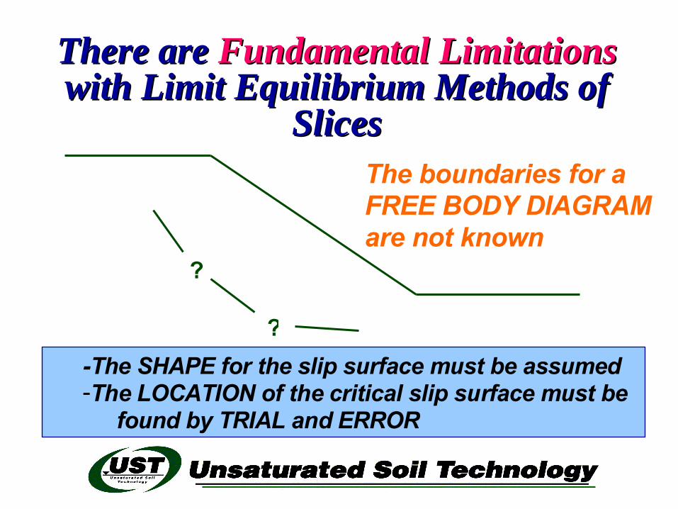
There are There are Fundamental LimitationsFundamental Limitations with Limit Equilibrium Methods of with Limit Equilibrium Methods of
SlicesSlices
?
?
The boundaries for a FREE BODY DIAGRAM are not known
-The SHAPE for the slip surface must be assumed-The LOCATION of the critical slip surface must be
found by TRIAL and ERROR
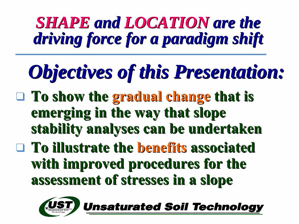
SHAPESHAPE and and LOCATIONLOCATION are the are the driving force for a paradigm shiftdriving force for a paradigm shift
Objectives of this Presentation:Objectives of this Presentation:❑ To show the To show the gradual changegradual change that is that is
emerging in the way that slope emerging in the way that slope stability analyses can be undertakenstability analyses can be undertaken
❑ To illustrate the To illustrate the benefitsbenefits associated associated with improved procedures for the with improved procedures for the assessment of stresses in a slopeassessment of stresses in a slope

Outline of PresentationOutline of Presentation Provide a brief Provide a brief SummarySummary of common of common
Limit Equilibrium methodsLimit Equilibrium methods along with along with their limitations (2-D & 3-D)their limitations (2-D & 3-D)
Take theTake the FIRSTFIRST step forward through step forward through use of an use of an independent stress analysisindependent stress analysis
Take the Take the SECONDSECOND step forward step forward through use of through use of Optimization Optimization TechniquesTechniques
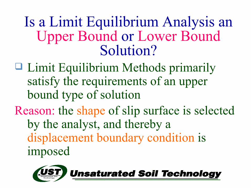
Is a Limit Equilibrium Analysis an Upper Bound or Lower Bound
Solution? Limit Equilibrium Methods primarily
satisfy the requirements of an upper bound type of solution
Reason: the shape of slip surface is selected by the analyst, and thereby a displacement boundary condition is imposed
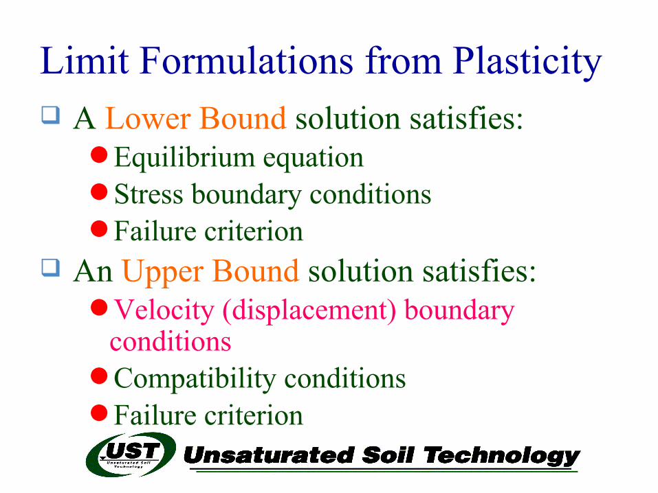
Limit Formulations from Plasticity A Lower Bound solution satisfies:
Equilibrium equationStress boundary conditionsFailure criterion
An Upper Bound solution satisfies:Velocity (displacement) boundary
conditionsCompatibility conditionsFailure criterion
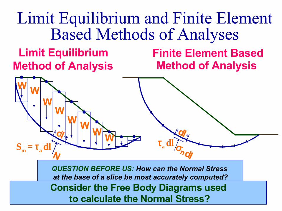
Limit Equilibrium and Finite Element Based Methods of Analyses
WW
W
WW W W W
N
Limit EquilibriumMethod of Analysis
Sm = τa dl
dlσndl
Finite Element Based Method of Analysis
ldτa dl
QUESTION BEFORE US: How can the Normal Stress at the base of a slice be most accurately computed?
Consider the Free Body Diagrams used to calculate the Normal Stress?
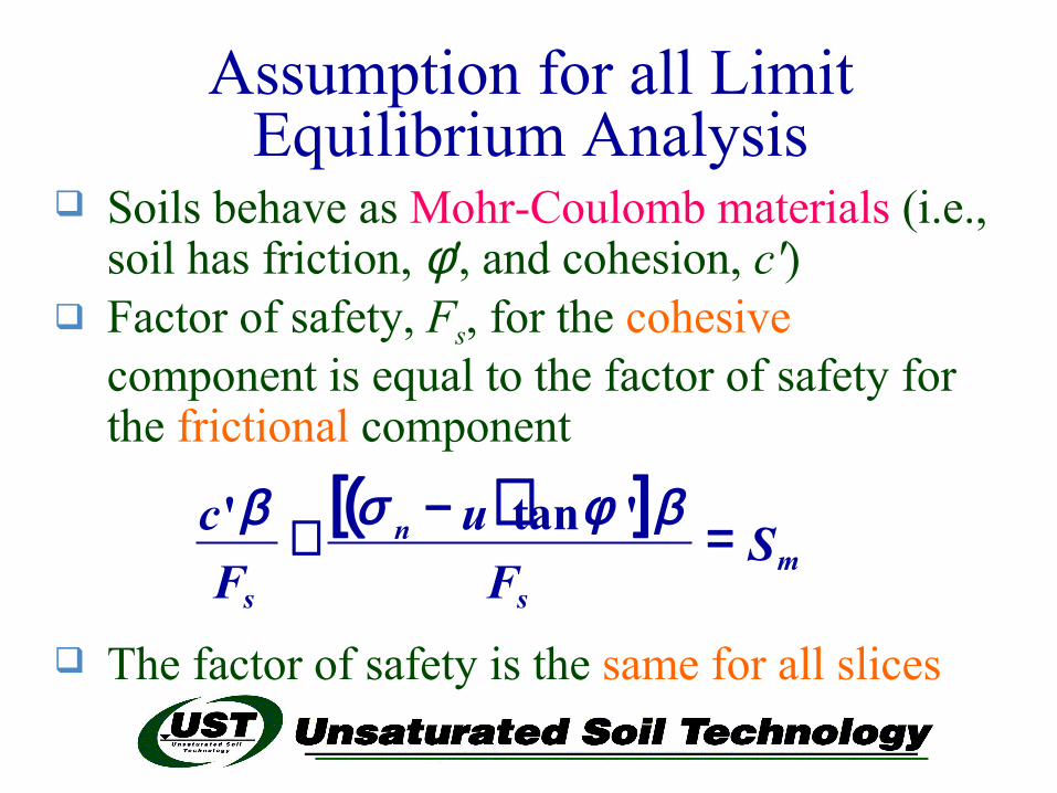
Assumption for all Limit Equilibrium Analysis
Soils behave as Mohr-Coulomb materials (i.e., soil has friction, φ', and cohesion, c')
Factor of safety, Fs, for the cohesive component is equal to the factor of safety for the frictional component
The factor of safety is the same for all slices
( )[ ]m
s
n
s
SF
uF
c =−+ βφσβ 'tan'
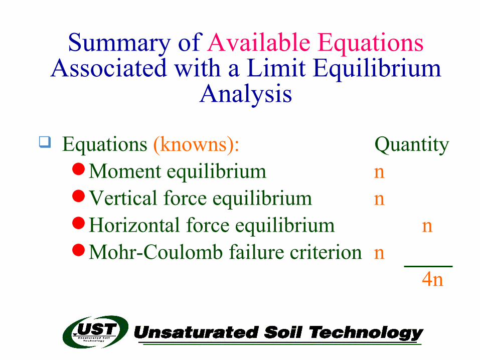
Summary of Available Equations Associated with a Limit Equilibrium
Analysis
Equations (knowns): QuantityMoment equilibrium nVertical force equilibrium nHorizontal force equilibrium nMohr-Coulomb failure criterion n
4n
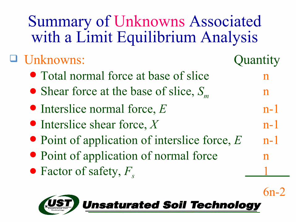
Unknowns: Quantity Total normal force at base of slice n Shear force at the base of slice, Sm n Interslice normal force, E n-1 Interslice shear force, X n-1 Point of application of interslice force, E n-1 Point of application of normal force n Factor of safety, Fs 1
6n-2
Summary of Unknowns Associated with a Limit Equilibrium Analysis
Definition of Factor of Safety, Fs
“That factor by which the shear strength parameters must be reduced to bring a soil mass into a state of limiting equilibrium along a given slip surface”
ss F'tanand
F'c φ
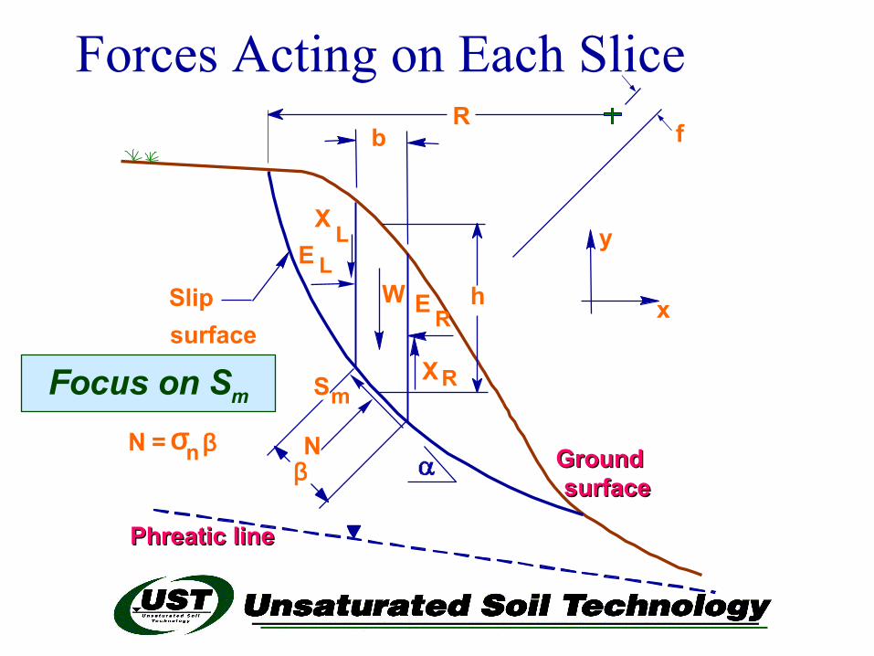
Forces Acting on Each Slice
Focus on Sm
b
y
x
SmXR
E R
EX L
Slip surface
Ground Ground surfacesurface
W h
R
N = σn ββ
f
N
L
Phreatic linePhreatic line
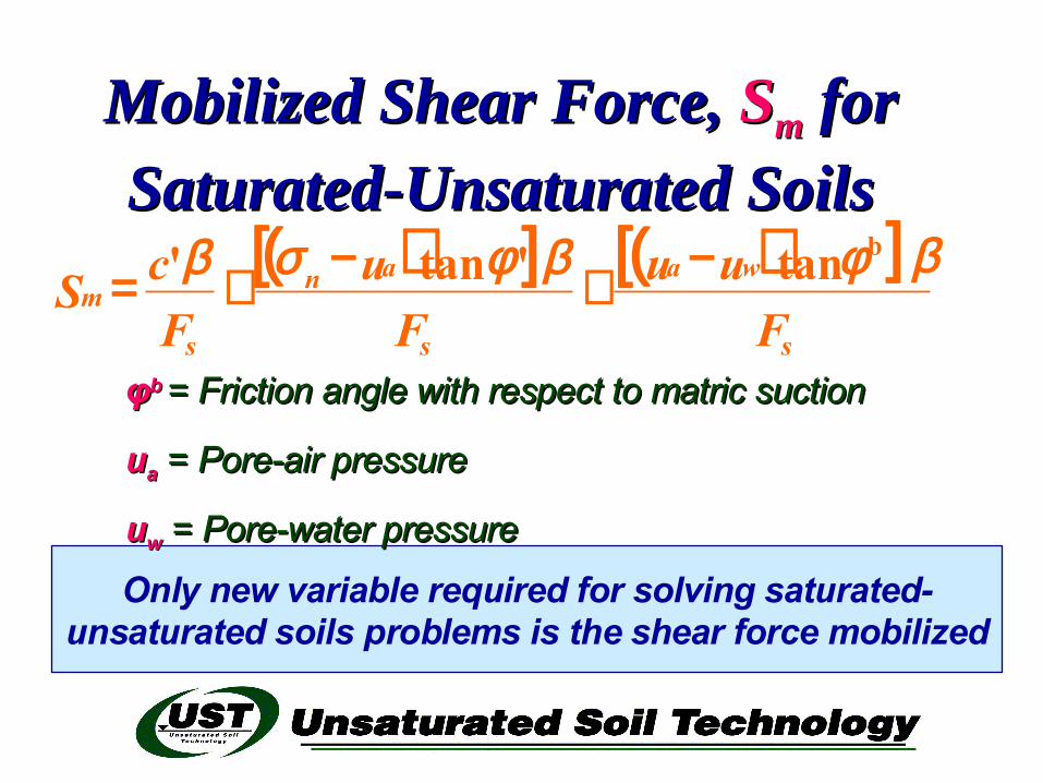
Mobilized Shear Force, Mobilized Shear Force, SSmm forforSaturated-Unsaturated SoilsSaturated-Unsaturated Soils
( )[ ] ( )s
wa
s
an
s
mF
uuF
uF
cSβφβφσβ btan'tan' −+−+=
Only new variable required for solving saturated-unsaturated soils problems is the shear force mobilized
φφbb = Friction angle with respect to matric suction= Friction angle with respect to matric suction
uuaa = Pore-air pressure = Pore-air pressure
uuww = Pore-water pressure= Pore-water pressure
[ ]
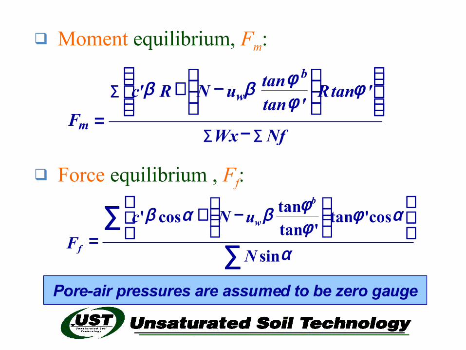
Moment equilibrium, Fm:
Force equilibrium , Ff:
∑ ∑
∑
−
−+
=NfWx
'tanR'tan
tanuNR'cF
b
w
m
φφφββ
∑∑
−+
=α
αφφφβαβ
sin
cos'tan'tan
tancos'
N
uNcF
b
w
f
Pore-air pressures are assumed to be zero gauge
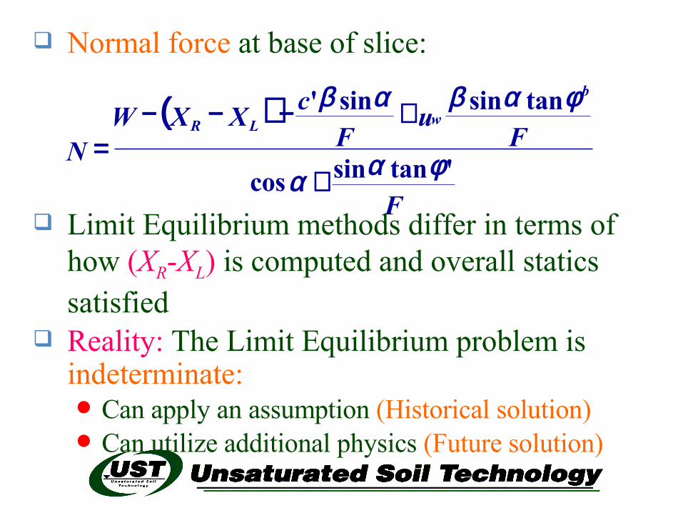
Normal force at base of slice:
Limit Equilibrium methods differ in terms of how (XR-XL) is computed and overall statics satisfied
Reality: The Limit Equilibrium problem is indeterminate: Can apply an assumption (Historical solution) Can utilize additional physics (Future solution)
( )
F
Fu
FcXXW
N
b
wLR
'tansincos
tansinsin'
φαα
φαβαβ
+
+−−−=
σx
b
a
Area = Interslice normal force (E)
width of slice, β
σxτxy
σy
Distance (m)
Ele
v atio
n (m
)
τxy
b
a
Area = Interslice shear force (X)
Vertical slice
Distance (m)
Ele
vati o
n ( m
)
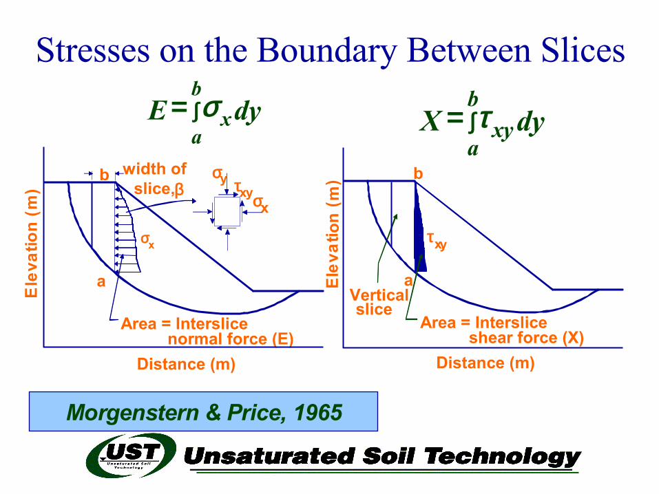
∫=b
axy dyX τ∫=
b
axdyE σ
Stresses on the Boundary Between Slices
Morgenstern & Price, 1965
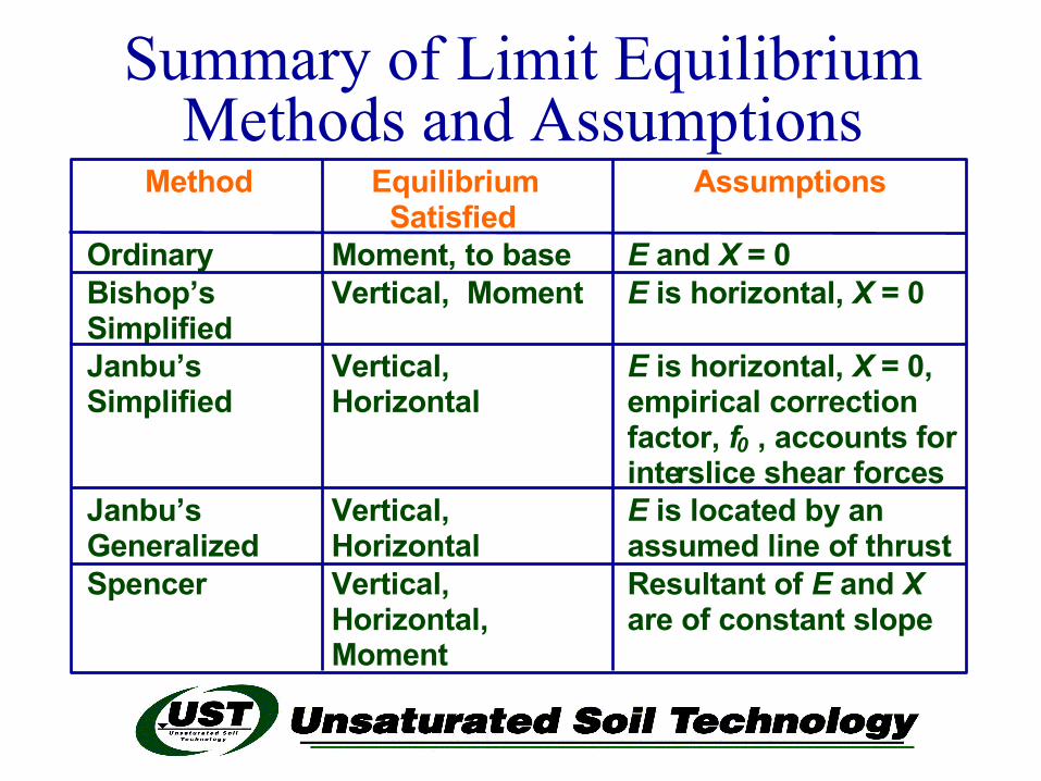
Summary of Limit Equilibrium Methods and Assumptions
Method Equilibrium Satisfied
Assumptions
Ordinary Moment, to base E and X = 0 Bishop’s Simplified
Vertical, Moment E is horizontal, X = 0
Janbu’s Simplified
Vertical, Horizontal
E is horizontal, X = 0, empirical correction factor, f0 , accounts for interslice shear forces
Janbu’s Generalized
Vertical, Horizontal
E is located by an assumed line of thrust
Spencer Vertical, Horizontal, Moment
Resultant of E and X are of constant slope
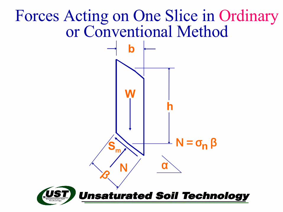
Forces Acting on One Slice in Ordinary or Conventional Method
hW
b
β α
Ν = σ β n
Ν
Sm
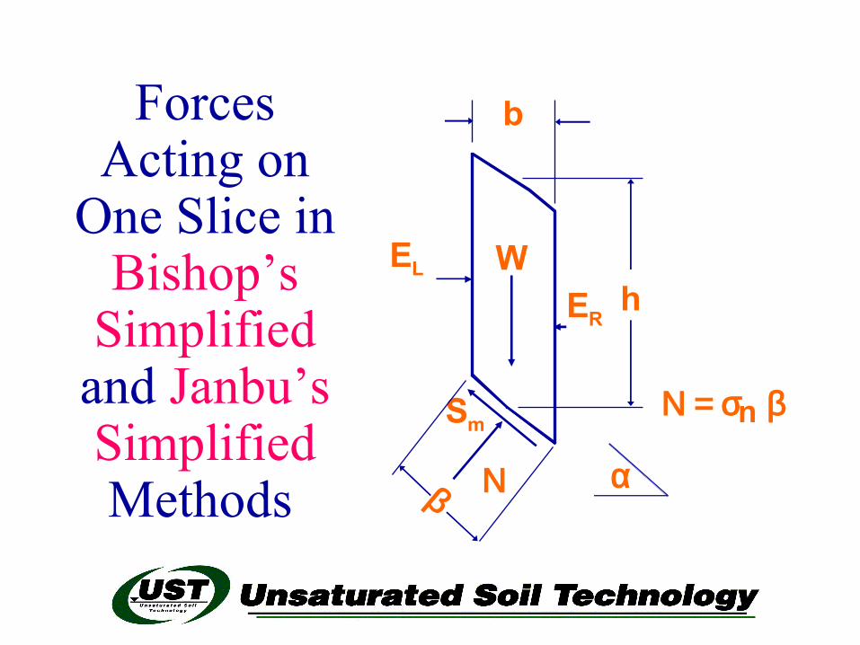
Forces Acting on
One Slice in Bishop’s
Simplified and Janbu’s Simplified Methods
hW
b
β α
Ν = σ β n
Ν
Sm
ER
EL
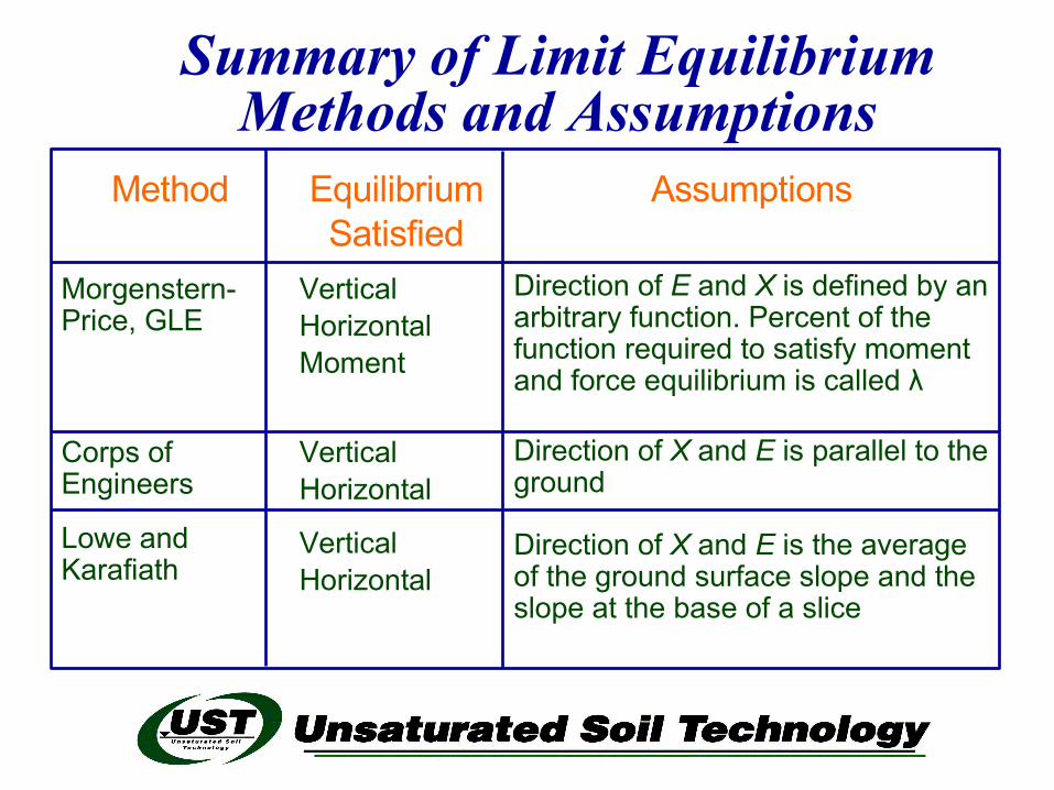
Summary of Limit Equilibrium Methods and Assumptions
Direction of X and E is the average of the ground surface slope and the slope at the base of a slice
VerticalHorizontal
Lowe and Karafiath
Direction of X and E is parallel to the ground
VerticalHorizontal
Corps of Engineers
Direction of E and X is defined by an arbitrary function. Percent of the function required to satisfy moment and force equilibrium is called λ
VerticalHorizontalMoment
Morgenstern-Price, GLE
AssumptionsEquilibriumSatisfied
Method
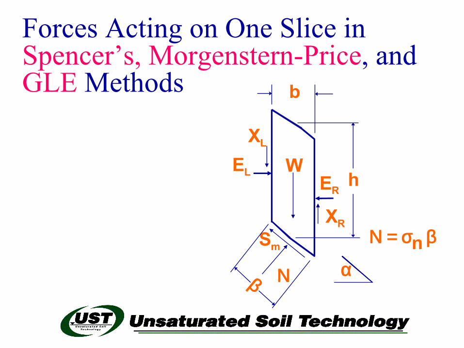
Forces Acting on One Slice in Spencer’s, Morgenstern-Price, andGLE Methods
hW
b
β α
Ν = σ β n
Ν
Sm
ER
EL
XR
XL
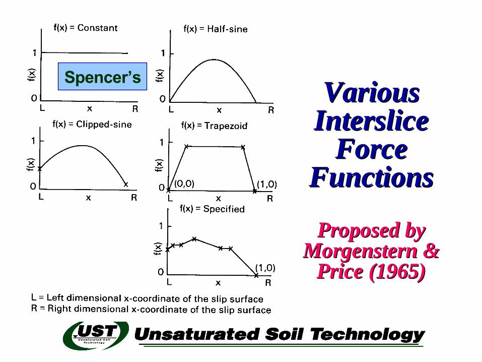
Various Various Interslice Interslice
Force Force FunctionsFunctions
Proposed byProposed byMorgenstern & Morgenstern &
Price (1965)Price (1965)
Spencer’s
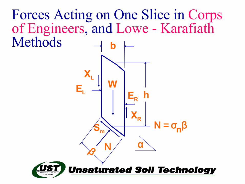
Forces Acting on One Slice in Corps of Engineers, and Lowe - Karafiath Methods
hW
b
β α
Ν = σ β n
Ν
Sm
EREL
XR
XL
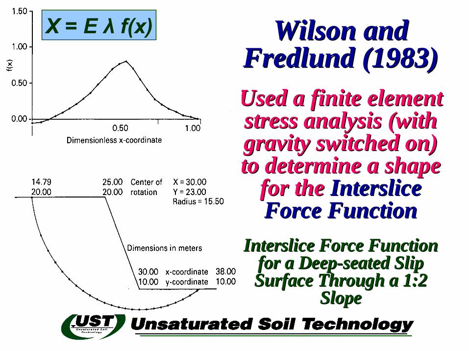
Wilson and Wilson and Fredlund (1983)Fredlund (1983)Used a finite element Used a finite element stress analysis (with stress analysis (with gravity switched on) gravity switched on) to determine a shape to determine a shape
for thefor the Interslice Interslice Force FunctionForce Function
Interslice Force Function Interslice Force Function for a Deep-seated Slip for a Deep-seated Slip Surface Through a 1:2 Surface Through a 1:2
SlopeSlope
X = E λ f(x)
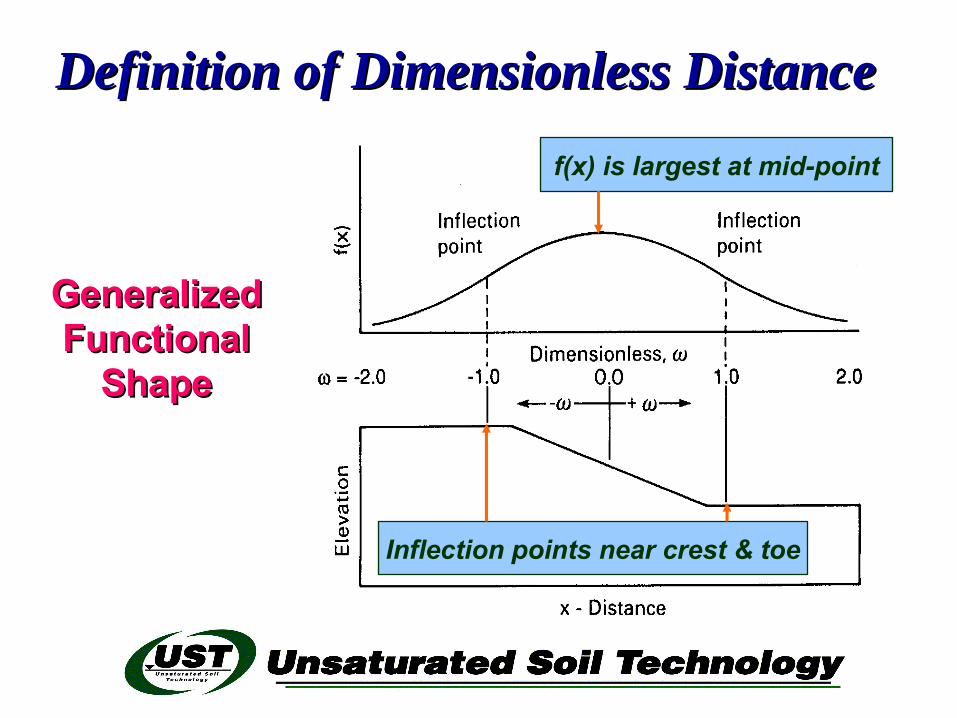
Definition of Dimensionless Distance Definition of Dimensionless Distance
f(x) is largest at mid-point
Inflection points near crest & toe
GeneralizedGeneralizedFunctionalFunctional
ShapeShape
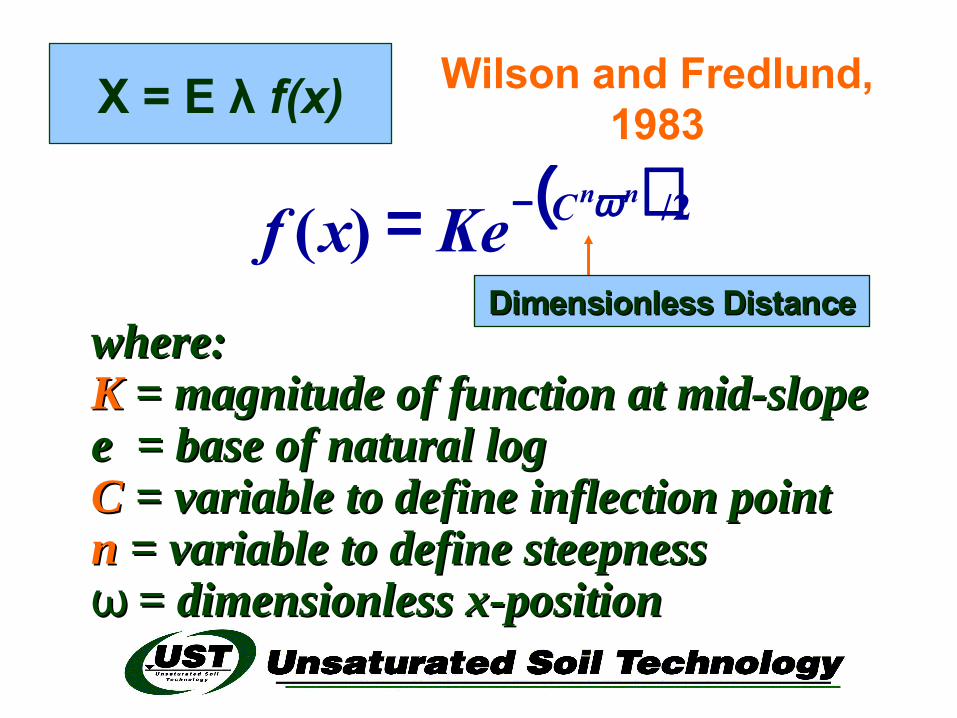
where:where:KK = magnitude of function at mid-slope = magnitude of function at mid-slopee = base of natural loge = base of natural logCC = variable to define inflection point = variable to define inflection pointn n = variable to define steepness= variable to define steepnessωω = dimensionless x-position = dimensionless x-position
( ) 2/)(nnCKexf ω−=
Wilson and Fredlund, 1983X = E λ f(x)
Dimensionless DistanceDimensionless Distance
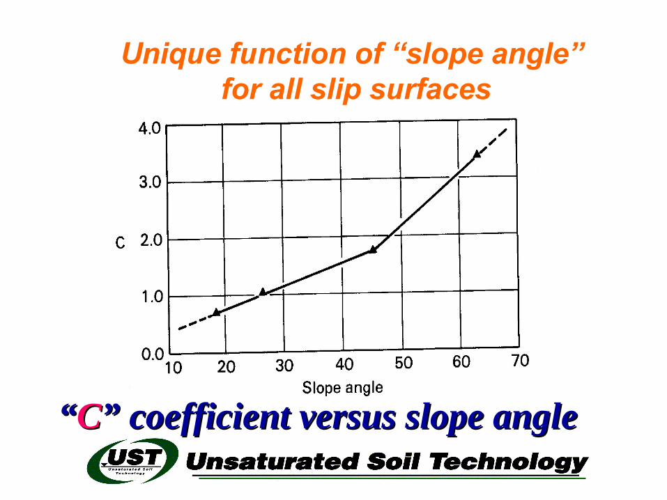
Unique function of “slope angle” for all slip surfaces
““CC” coefficient versus slope angle” coefficient versus slope angle
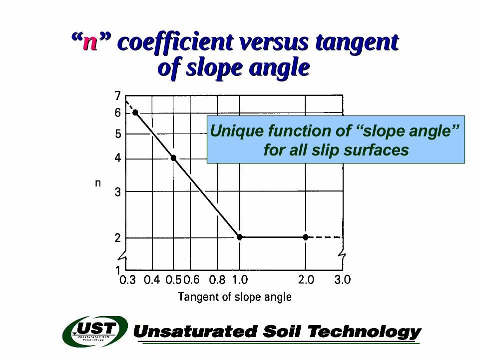
Unique function of “slope angle” for all slip surfaces
““nn” coefficient versus tangent ” coefficient versus tangent of slope angleof slope angle
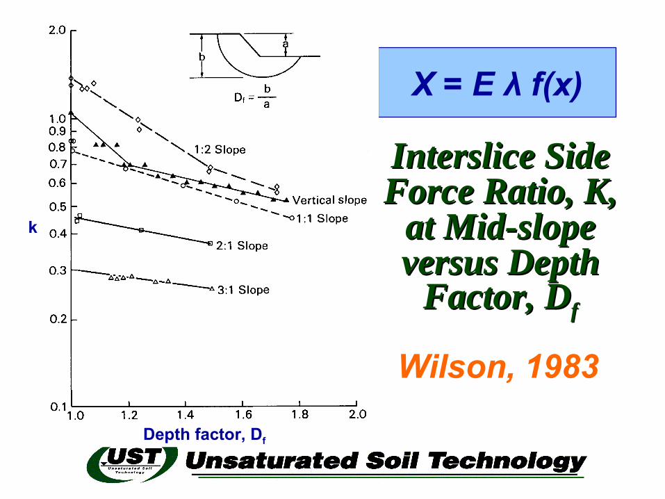
Interslice Side Interslice Side Force Ratio, K, Force Ratio, K,
at Mid-slope at Mid-slope versus Depth versus Depth
Factor, DFactor, Dff
Wilson, 1983
X = E λ f(x)
Depth factor, Df
k
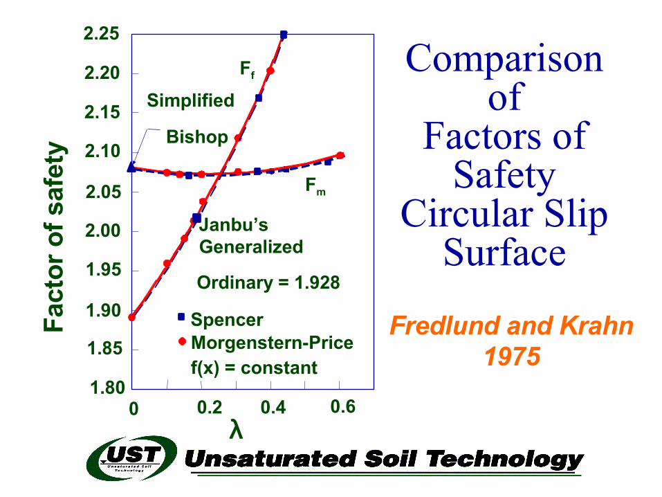
Comparison of
Factors of Safety
Circular Slip Surface
0 0.2 0.4 0.61.80
1.85
1.90
1.95
2.00
2.05
2.10
2.15
2.20
2.25
λ
Janbu’s Generalized
Simplified
Bishop
SpencerMorgenstern-Pricef(x) = constant
Ordinary = 1.928
Ff
Fm
Fredlund and Krahn1975
Fact
or o
f saf
ety
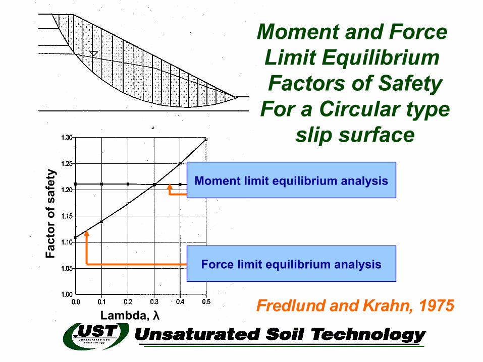
Moment and Force Limit Equilibrium Factors of Safety
For a Circular typeslip surface
Moment limit equilibrium analysis
Force limit equilibrium analysis
Fredlund and Krahn, 1975Lambda, λ
Fact
or o
f saf
ety
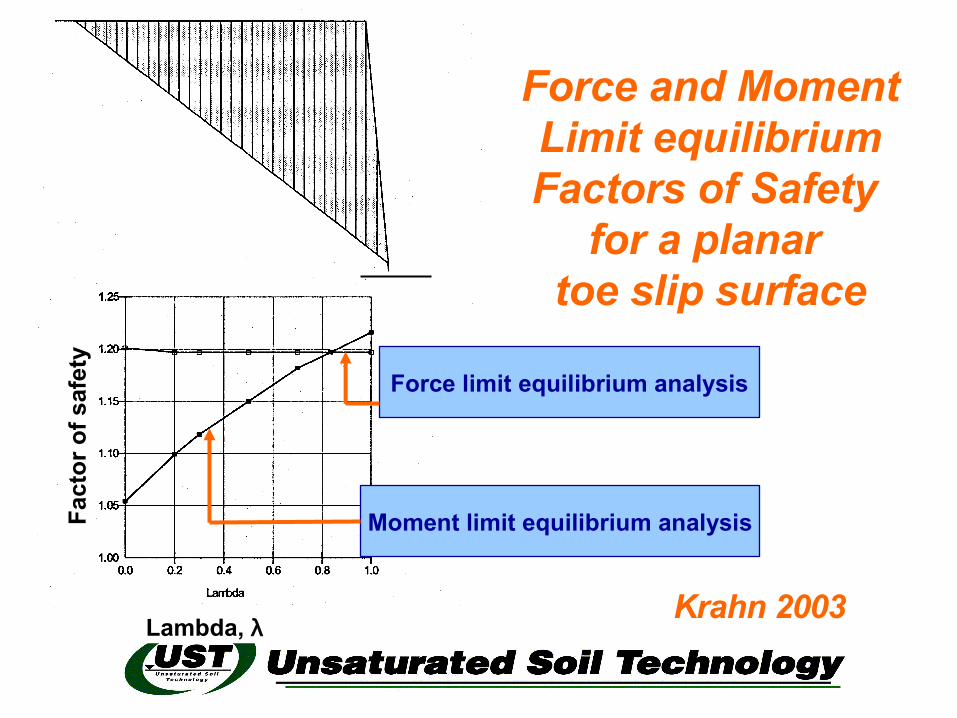
Force and MomentLimit equilibriumFactors of Safety
for a planar toe slip surface
Force limit equilibrium analysis
Moment limit equilibrium analysis
Lambda, λ
Fact
or o
f saf
ety
Krahn 2003
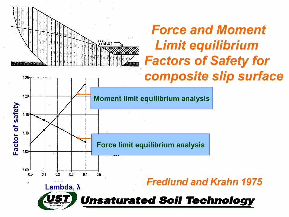
Force and MomentLimit equilibrium
Factors of Safety for a composite slip surface
Moment limit equilibrium analysis
Force limit equilibrium analysis
Lambda, λ
Fact
or o
f saf
ety
Fredlund and Krahn 1975
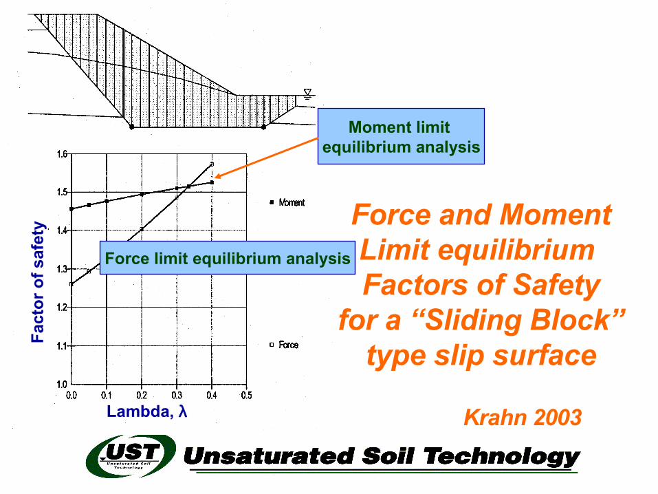
Force and MomentLimit equilibrium Factors of Safety
for a “Sliding Block” type slip surface
Moment limit equilibrium analysis
Force limit equilibrium analysis
Lambda, λ
Fact
or o
f saf
ety
Krahn 2003
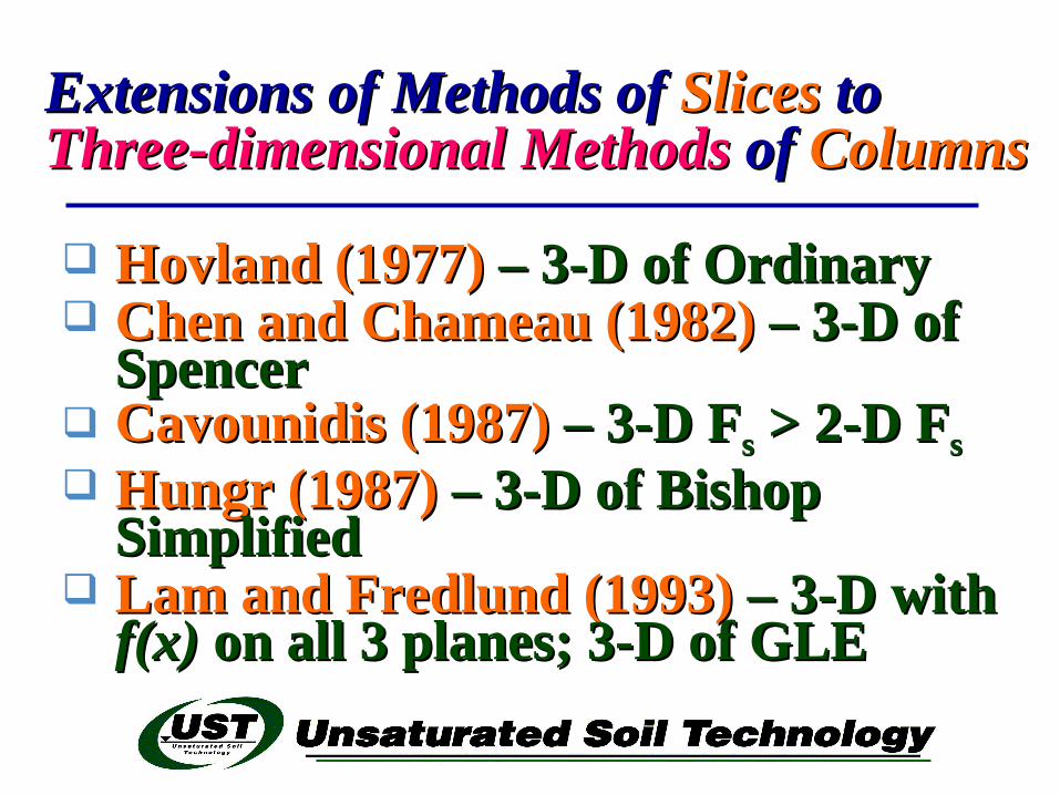
Extensions of Methods of Extensions of Methods of Slices Slices totoThree-dimensional MethodsThree-dimensional Methods of of ColumnsColumns
Hovland (1977)Hovland (1977) – 3-D of Ordinary – 3-D of Ordinary Chen and Chameau (1982)Chen and Chameau (1982) – 3-D of – 3-D of
Spencer Spencer Cavounidis (1987)Cavounidis (1987) – 3-D F – 3-D Fss > 2-D F > 2-D Fss Hungr (1987)Hungr (1987) – 3-D of Bishop – 3-D of Bishop
SimplifiedSimplified Lam and Fredlund (1993)Lam and Fredlund (1993) – 3-D with – 3-D with
f(x)f(x) on all 3 planes; 3-D of GLE on all 3 planes; 3-D of GLE
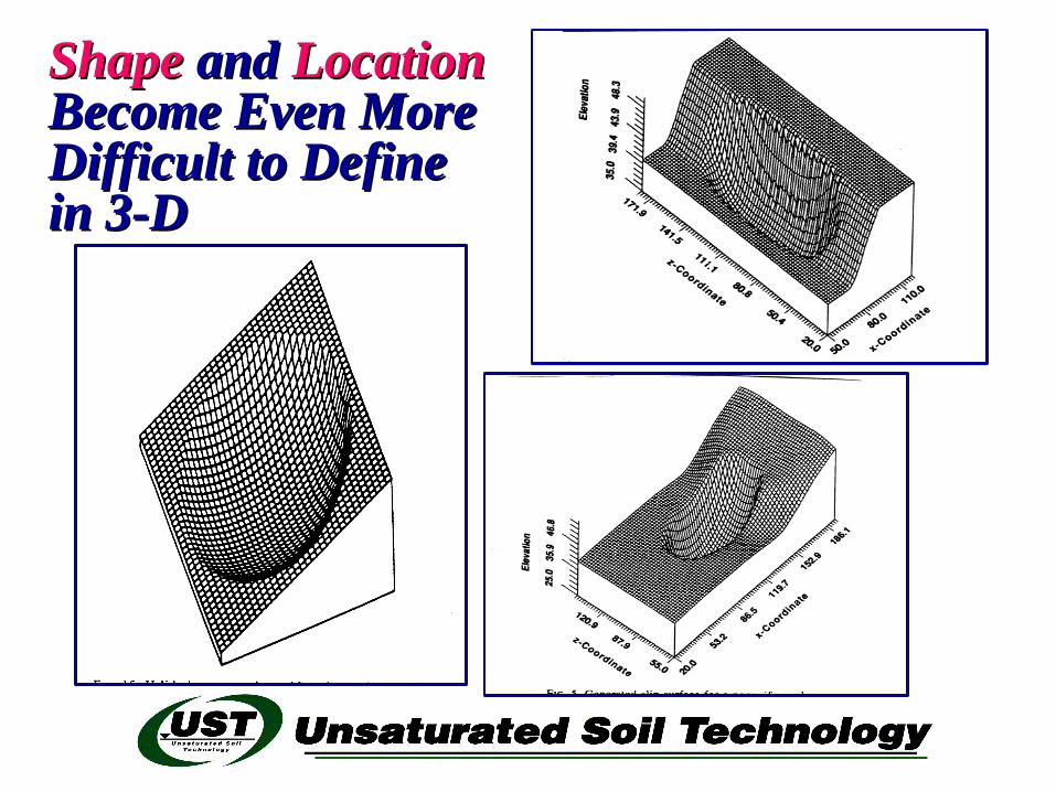
ShapeShape and and Location Location Become Even More Become Even More Difficult to Define Difficult to Define in 3-Din 3-D
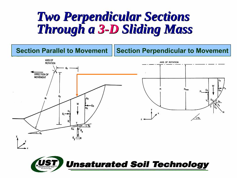
Two Perpendicular Sections Two Perpendicular Sections Through a Through a 3-D3-D Sliding MassSliding Mass
Section Parallel to Movement Section Perpendicular to Movement
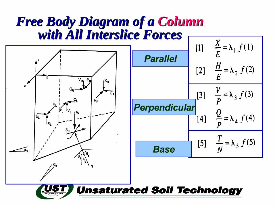
Free Body Diagram of a Free Body Diagram of a Column Column with All Interslice Forceswith All Interslice Forces
Parallel
Perpendicular
Base
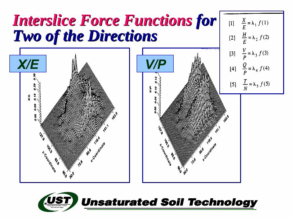
Interslice Force FunctionsInterslice Force Functions for for Two of the DirectionsTwo of the Directions
X/E V/P
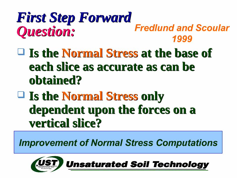
First Step ForwardFirst Step ForwardQuestion:Question: Is the Is the Normal StressNormal Stress at the base of at the base of
each slice as accurate as can be each slice as accurate as can be obtained?obtained?
Is the Is the Normal StressNormal Stress only only dependent upon the forces on a dependent upon the forces on a vertical slice?vertical slice?
Improvement of Normal Stress Computations
Fredlund and Scoular1999
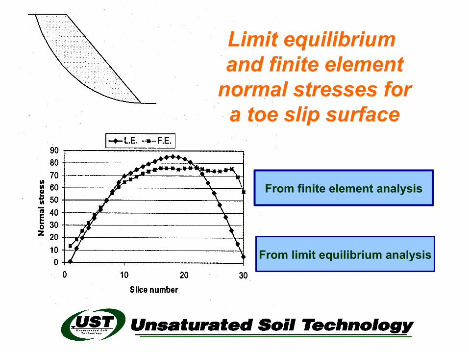
Limit equilibrium and finite element
normal stresses for a toe slip surface
From limit equilibrium analysis
From finite element analysis
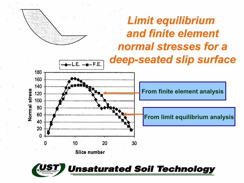
Limit equilibrium and finite element
normal stresses for a deep-seated slip surface
From finite element analysis
From limit equilibrium analysis
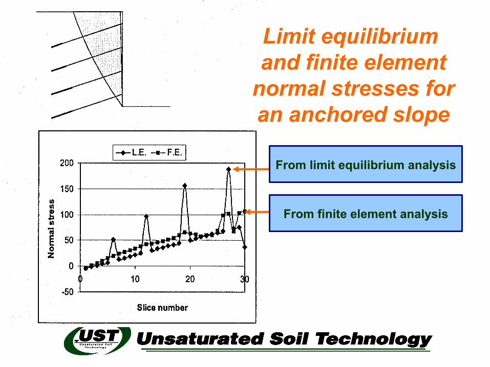
Limit equilibrium and finite element
normal stresses for an anchored slope
From finite element analysis
From limit equilibrium analysis
To illustrate procedures for combining a finite element stress analysis with concepts of limiting equilibrium. (i.e., finite element method of slope stability analysis)
To compare results of a finite element slope stability analysis and conventional limit equilibrium methods
Using Limit Equilibrium Concepts in a Finite Element Slope Stability Analysis
Objective:
The complete stress state from a finite element analysis can be “imported” into a limit equilibrium framework where the normal stress and the actuating shear stress are computed for any selected slip surface
Hypothesis
Assumption: The stresses computed from“switching-on” gravity are more reasonable than
the stresses computed on a vertical slice
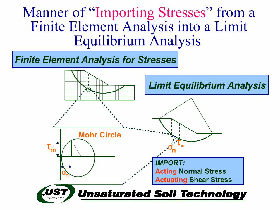
Manner of “Importing Stresses” from a Finite Element Analysis into a Limit
Equilibrium Analysis
σn
Finite Element Analysis for Stresses
Limit Equilibrium Analysis
σnτm
Mohr Circleτm
IMPORT:Acting Normal StressActuating Shear Stress
Limit Equilibrium Analysis
Finite Element Analysis for Stresses
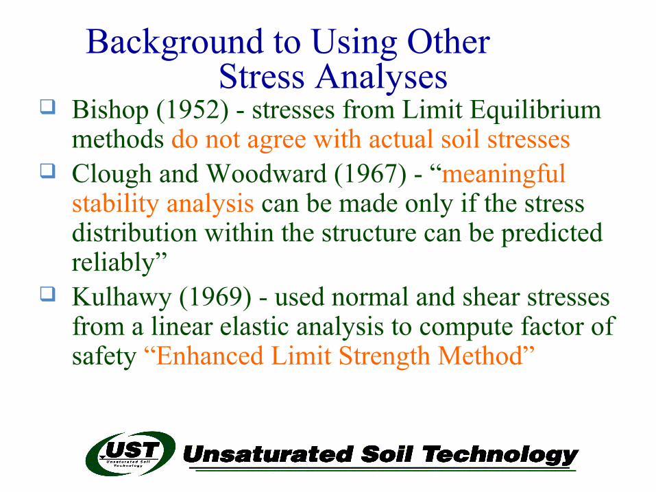
Bishop (1952) - stresses from Limit Equilibrium methods do not agree with actual soil stresses
Clough and Woodward (1967) - “meaningful stability analysis can be made only if the stress distribution within the structure can be predicted reliably”
Kulhawy (1969) - used normal and shear stresses from a linear elastic analysis to compute factor of safety “Enhanced Limit Strength Method”
Background to Using Other Stress Analyses
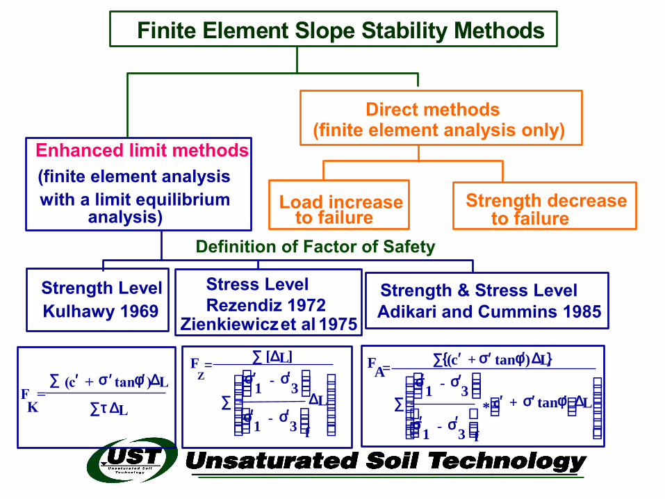
Stress LevelRezendiz 1972
Zienkiewicz et al 1975
Strength & Stress LevelAdikari and Cummins 1985
Enhanced limit methods(finite element analysiswith a limit equilibrium
Finite Element Slope Stability Methods
Direct methods(finite element analysis only)
Strength LevelKulhawy 1969
F [ ]
-
-
Z =
1 3
1 3
∑′ ′
′ ′∑
∆
∆
L
L
f
σ σ
σ σ
{ }F = (c + tan )
-
-
c + tan
A 1 3
1 3
′ ′ ′∑′ ′
′ ′′ ′ ′∑
σ φσ σ
σ σσ φ
∆
∆
L
L
f
*F =
(c + tan )
K
∑ ′ ′ ′
∑
σ φ
τ
∆
∆
L
L
Definition of Factor of Safety
Load increaseto failure
Strength decreaseto failureanalysis)
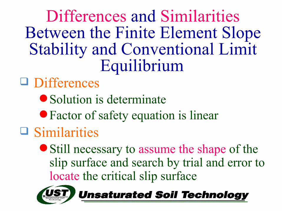
Differences and Similarities Between the Finite Element Slope Stability and Conventional Limit
Equilibrium
DifferencesSolution is determinateFactor of safety equation is linear
SimilaritiesStill necessary to assume the shape of the
slip surface and search by trial and error to locate the critical slip surface
Why hasn’t Finite Element Slope Stability Method been
extensively used?
Difficulties and perceptions related to the stress analysis
Inability to transfer large amounts of data and find needed information
Now: Microcomputer have dramatically changed our ability to combine Finite Element and Limit Equilibrium analyses
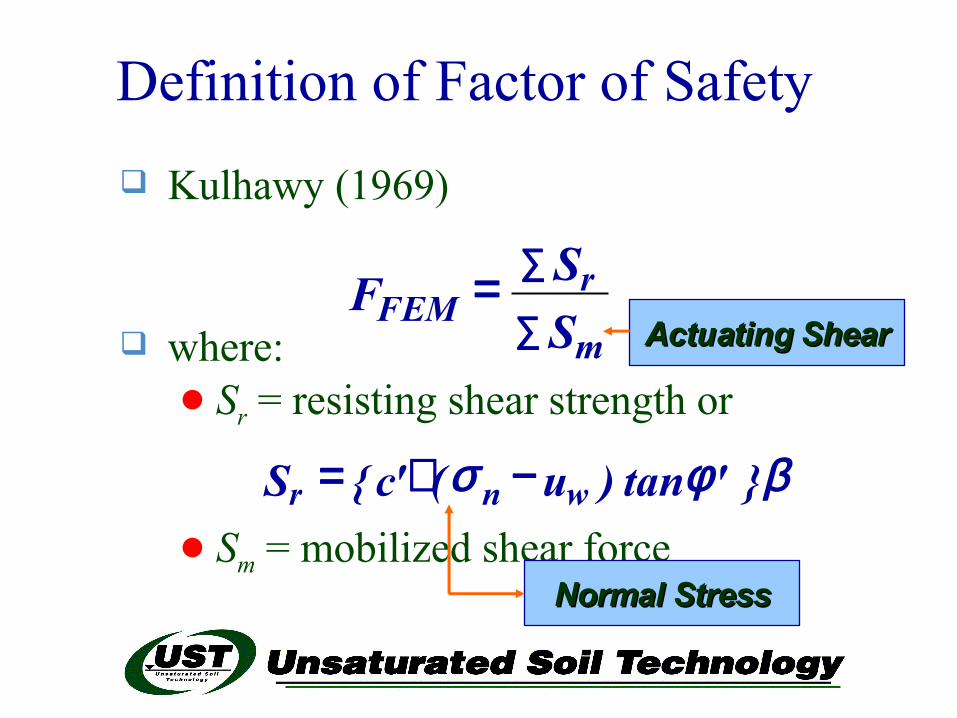
Definition of Factor of Safety
Kulhawy (1969)
where: Sr = resisting shear strength or
Sm = mobilized shear force
∑
∑=m
rFEM S
SF
βφσ }'tan)u('c{S wnr −+=
Actuating ShearActuating Shear
Normal StressNormal Stress

Analysis Study Undertaken by Fredlund and Scoular (1999)
Adopted the Kulhawy (1969) procedure Used Sigma/W and Slope/W Poisson’s ratio range = 0.33 to 0.48 Elastic modulus, E = 20,000 to 200,000 kPa Cohesion, c' = 10 to 40 kPa Friction, φ' = 10 to 30 degrees Compared conventional Limit Equilibrium
results with Finite Element slope stability results
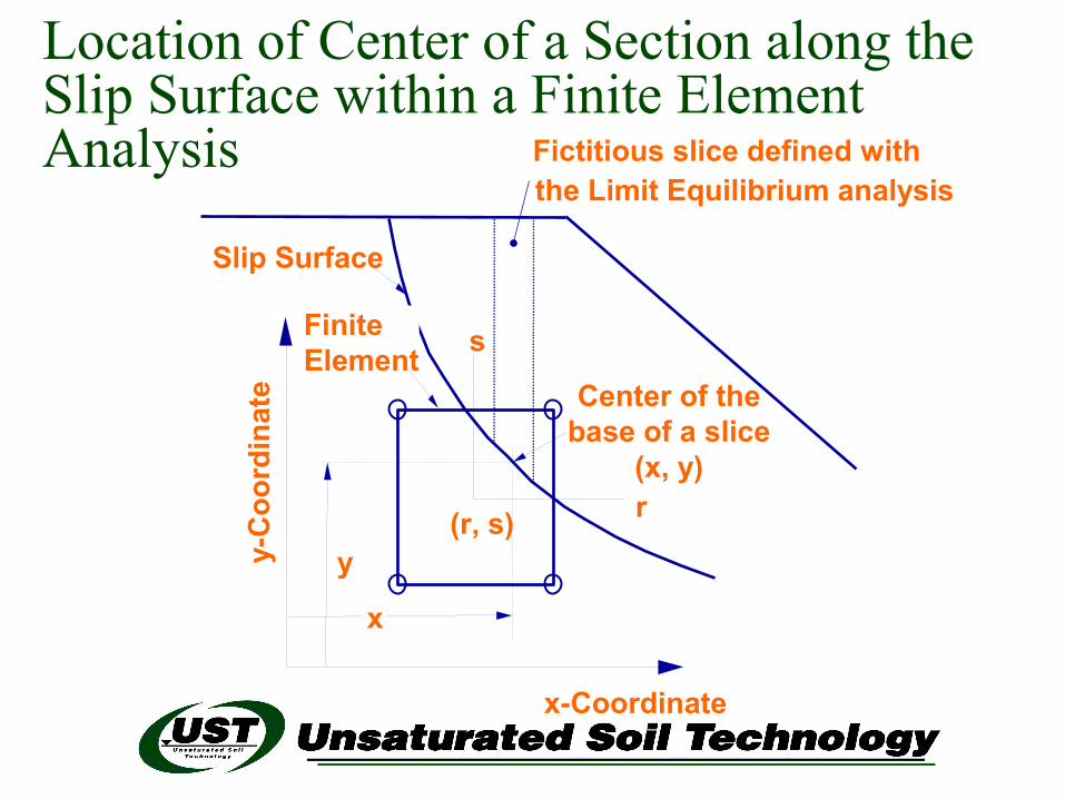
Location of Center of a Section along the Slip Surface within a Finite Element Analysis
x
y
x-Coordinate
y-C
oord
inat
eSlip Surface
Finite Element
(r, s)
s
r
Fictitious slice defined withthe Limit Equilibrium analysis
Center of the base of a slice
(x, y)
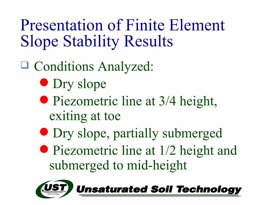
Presentation of Finite Element Slope Stability Results
Conditions Analyzed: Dry slope Piezometric line at 3/4 height,
exiting at toe Dry slope, partially submerged Piezometric line at 1/2 height and
submerged to mid-height
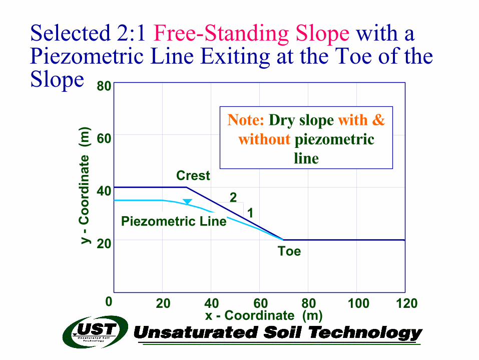
Selected 2:1 Free-Standing Slope with a Piezometric Line Exiting at the Toe of the Slope
20 40 60 80 100 120
20
40
60
80
0
Crest
Piezometric Line
Toe
21
x - Coordinate (m)
Note: Dry slope with & without piezometric
line
y - C
oord
inat
e (m
)
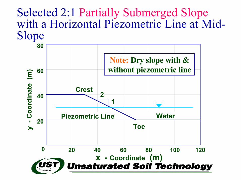
Selected 2:1 Partially Submerged Slope with a Horizontal Piezometric Line at Mid-Slope
20 40 60 80 100 120
20
40
60
80
0
Crest
Toe
21
x - Coordinate (m)
WaterPiezometric Line
y -
Coo
rdin
ate
(m)
Note: Dry slope with & without piezometric line
050
100
150200
250
300
20 30 40 50 60 70x-Coordinate (m)
Act
ing
and
rest
rict
ing
shea
r st
ress
(kPa
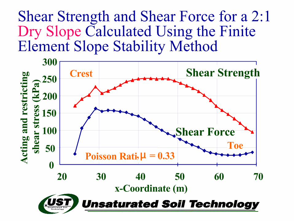
) Crest
Toe
Shear Strength
Shear Force
Poisson Ratio, µ = 0.33
Shear Strength and Shear Force for a 2:1 Dry Slope Calculated Using the Finite Element Slope Stability Method
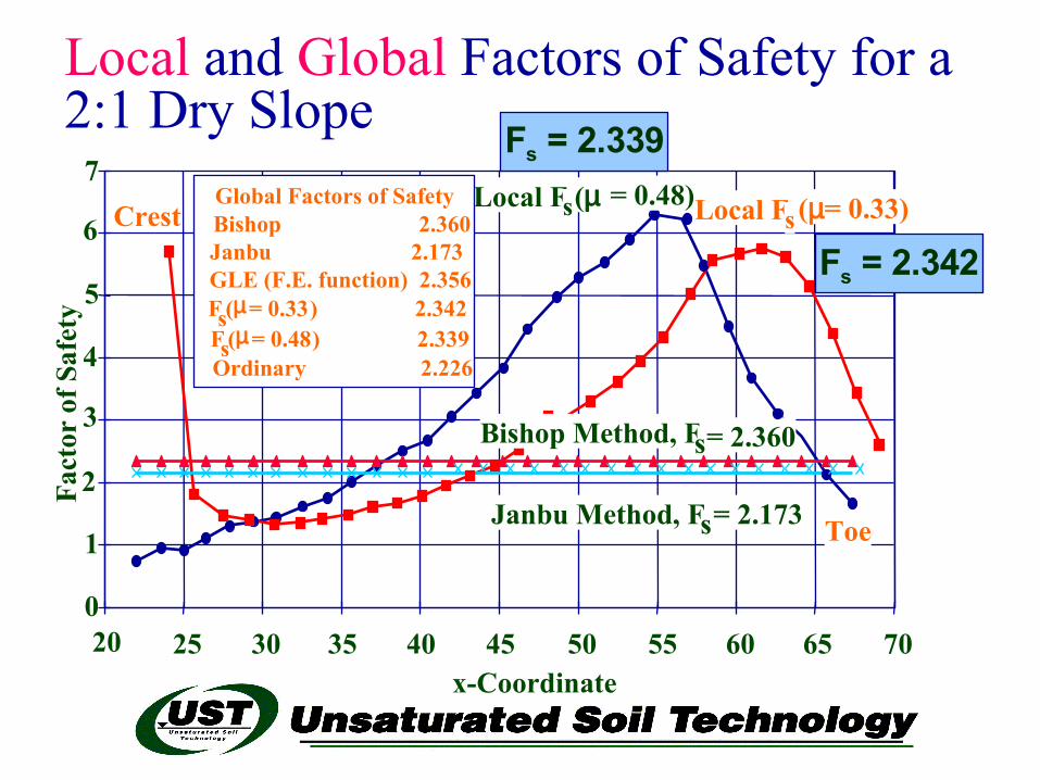
Local and Global Factors of Safety for a 2:1 Dry Slope
0
1
2
3
4
5
6
7
20 25 30 35 40 45 50 55 60 65 70x-Coordinate
Fact
or o
f Saf
ety
Crest
Toe
Local F (µ Local F (µ= 0.33)
Bishop Method, F = 2.360
= 2.173
Global Factors of SafetyBishop 2.360Janbu 2.173GLE (F.E. function) 2.356Fs (µ = 0.33 ) 2.342Fs (µ = 0.48 ) 2.339Ordinary 2.226
s
Janbu Method, Fs
s
s
Fs = 2.342
Fs = 2.339 = 0.48)
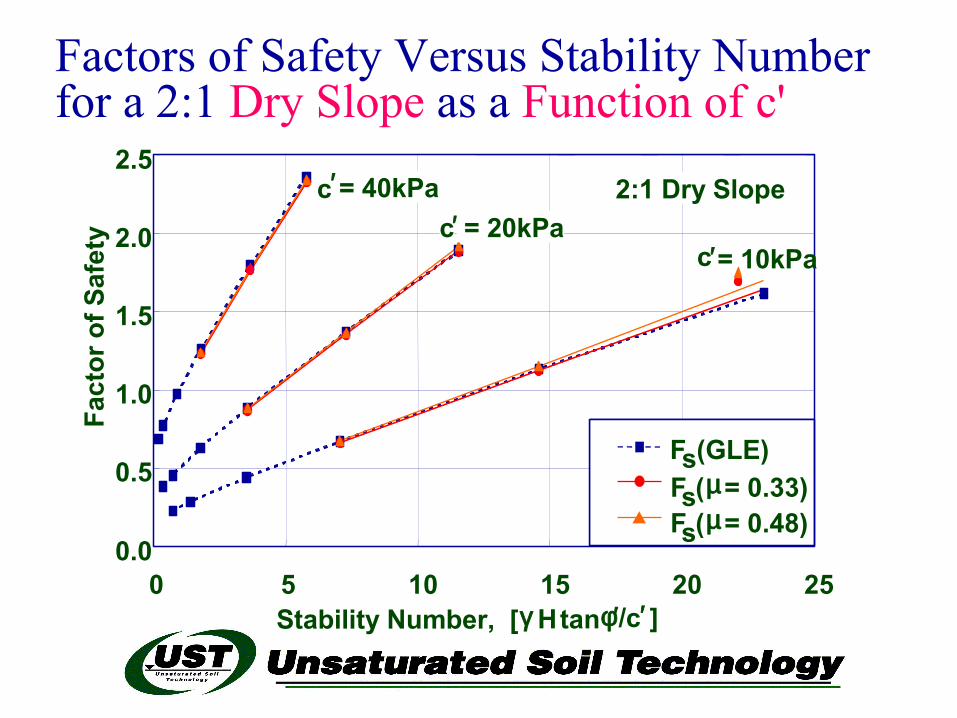
Factors of Safety Versus Stability Number for a 2:1 Dry Slope as a Function of c'
0.0
0.5
1.0
1.5
2.0
2.5
0 5 10 15 20 25Stability Number, [γ Htan φ′ /c′ ]
Fact
or o
f Saf
ety c′ = 20kPa
c′ = 10kPa
c = 40kPa
Fs ( µ = 0.33)Fs ( µ = 0.48)
Fs (GLE)
2:1 Dry Slope′
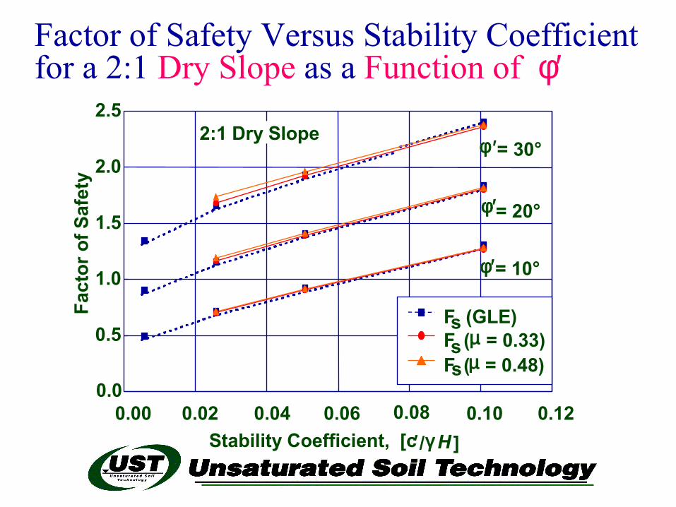
Factor of Safety Versus Stability Coefficient for a 2:1 Dry Slope as a Function of φ′
0.0
0.5
1.0
1.5
2.0
2.5
0.00 0.02 0.04 0.06 0.08 0.10 0.12Stability Coefficient, [c ′/γ H ]
Fact
or o
f Saf
ety
φ ′= 30°
φ′ = 10°
φ′= 20°
2:1 Dry Slope
sFs ( µ = 0.33)F (µ = 0.48)
Fs (GLE)
s
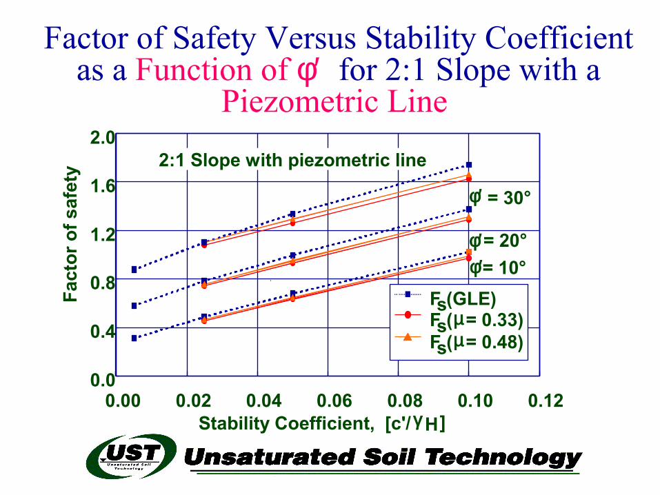
Factor of Safety Versus Stability Coefficient as a Function of φ′ for 2:1 Slope with a
Piezometric Line
0.0
0.4
0.8
1.2
1.6
2.0
0.00 0.02 0.04 0.06 0.08 0.10 0.12Stability Coefficient, [c'/ γ H ]
Fact
or o
f saf
ety
φ′ = 30°
φ′ = 20°φ′ = 10°
2:1 Slope with piezometric line
Fs ( µ = 0.33)Fs ( µ = 0.48)
Fs (GLE)
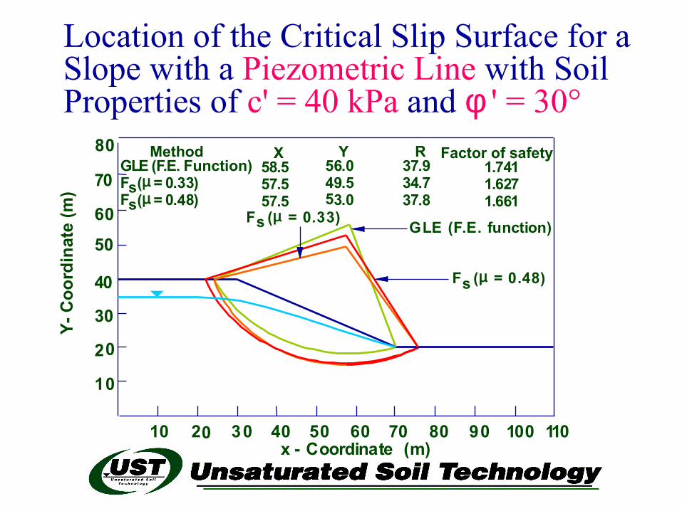
Location of the Critical Slip Surface for a Slope with a Piezometric Line with Soil Properties of c' = 40 kPa and φ ' = 30°
70
10 20 10060504030 908070 110
50
60
40
10
20
30
x - Coordinate (m)
80
GLE (F.E. function)Fs (µ = 0.33)
Fs (µ = 0.48)
Method X Y R Factor of safetyGLE (F.E. Function) 58.5 56.0 37.9 1.741Fs (µ = 0.33) 57.5 49.5 34.7 1.627Fs (µ = 0.48) 57.5 53.0 37.8 1.661
Y- C
oord
inat
e (m
)
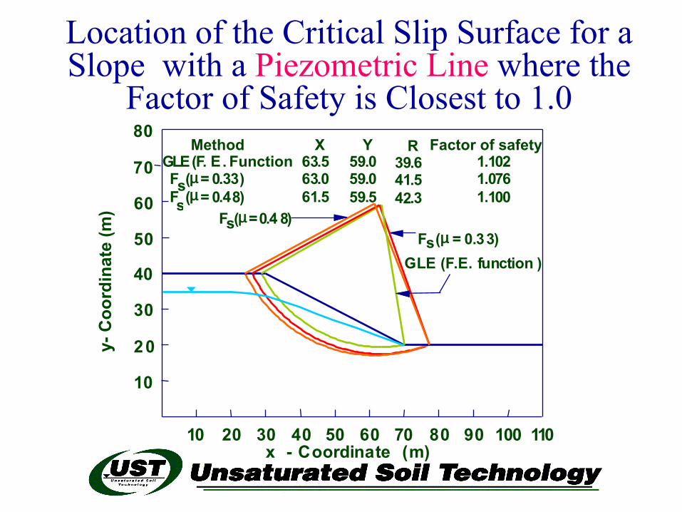
Location of the Critical Slip Surface for a Slope with a Piezometric Line where the
Factor of Safety is Closest to 1.0
70
10 20 10060504030 908070
50
60
40
10
20
30
110x - Coordinate (m)
80
Fs (µ = 0.4 8 )Fs (µ = 0.33)
GLE (F.E. function )
s
Method X Y R Factor of safetyGLE (F. E Function . 63.5 59.0 39.6 1.102Fs (µ = 0.33) 63.0 59.0 41.5 1.076F (µ = 0.48) 61.5 59.5 42.3 1.100
y- C
oord
inat
e (m
)
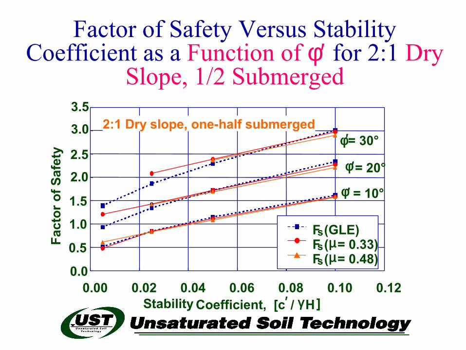
Factor of Safety Versus Stability Coefficient as a Function of φ′ for 2:1 Dry
Slope, 1/2 Submerged
0.0
0.5
1.0
1.5
2.02.5
3.03.5
0.00 0.02 0.04 0.06 0.08 0.10 0.12Stability Coefficient, [c ′ / γ H]
Fact
or o
f Saf
ety
φ′ = 20°
φ ′ = 10°
2:1 Dry slope, one-half submergedφ′ = 30°
Fs ( µ = 0.33)Fs ( µ = 0.48)
Fs (GLE)
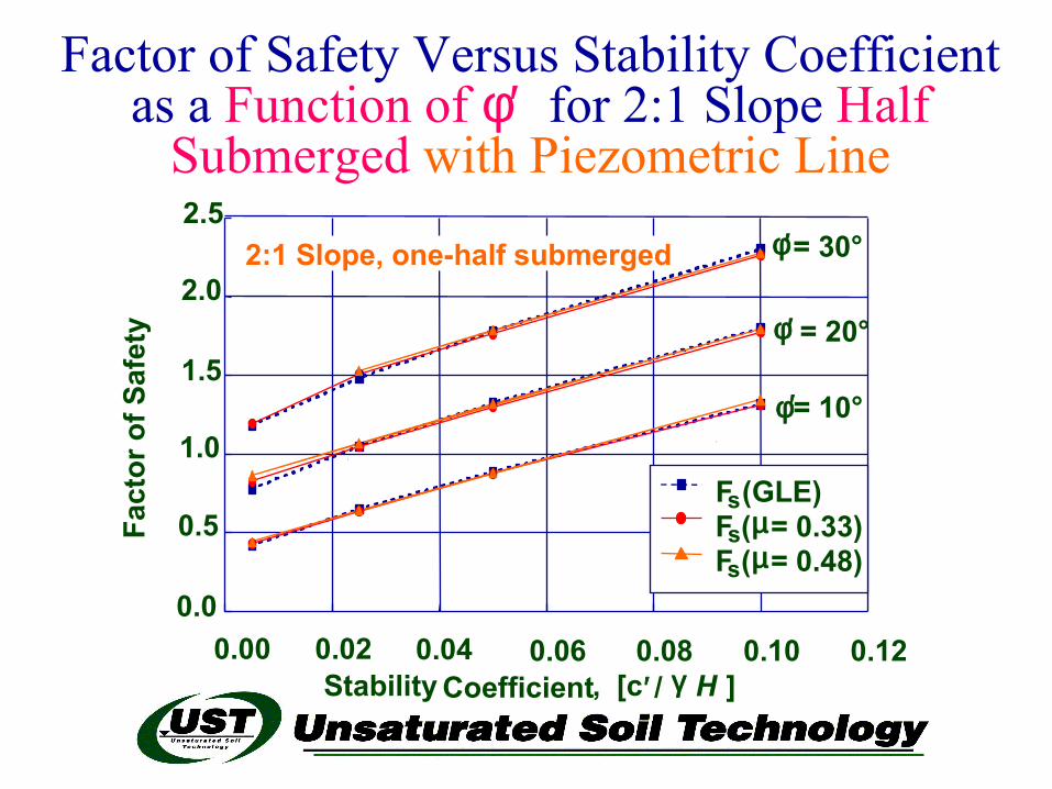
Factor of Safety Versus Stability Coefficient as a Function of φ′ for 2:1 Slope Half
Submerged with Piezometric Line
0.0
0.5
1.0
1.5
2.0
2.5
0.00 0.02 0.04 0.06 0.08 0.10 0.12Stability Coefficient , [c′ / H ]
Fact
or o
f Saf
ety
φ′ = 30°
φ′= 10°
φ′ = 20°
2:1 Slope, one-half submerged
γ
Fs ( µ = 0.33)Fs ( µ = 0.48)
Fs (GLE)
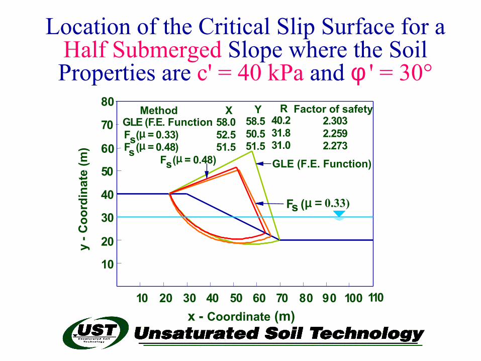
10 20 10060504030 908070 110
70
50
60
40
10
20
30
80
Fs (µ = 0.33)
Fs (µ = 0.48) GLE (F.E. Function)s
Method X Y R Factor of safetyGLE (F.E. Function 58.0 58.5 40.2 2.303Fs (µ = 0.33) 52.5 50.5 31.8 2.259F (µ = 0.48) 51.5 51.5 31.0 2.273
Location of the Critical Slip Surface for a Half Submerged Slope where the Soil Properties are c' = 40 kPa and φ ' = 30°
x - Coordinate (m)
y - C
oord
inat
e (m
)
Conclusions from Step 1 Forward Normal and Actuating Shear stresses from a
finite element analysis appears to provide a more accurate representation of the stress state in a slope
The Enhanced Limit method by Kulhawy (1969) appears to open the way to simulate more complex slope stability problems
Enhanced Limit methods can readily be used in routine engineering practice
Global factors of safety appear to be essentially the same for most simple slopes
Selection of Poisson’s ratio has some effect on the Enhanced Limit factor of safety
Factors of Safety appear to differ slightly for:Low cohesion valuesHigh angles of internal friction
How do the Results from Enhanced Limit Methods Compare to Limit
Equilibrium Methods?
Local Factors of Safety can also be computed by the Enhanced Limit Method
Second Step ForwardSecond Step Forward
Question:Question: Is it possible for the computer to Is it possible for the computer to
determine the determine the ShapeShape of the critical of the critical slip surface?slip surface?
Is it possible for the computer to Is it possible for the computer to determine the determine the Location Location of the of the critical slip surface?critical slip surface?
Improvement on Shape and Location
Ha and Fredlund2002
Optimization Techniques (i.e., Dynamic Programming) can be used to find the pathway which minimizes a function of the shear strength available to the actuating shear stress within a soil mass
Hypothesis
Assumption: The stresses computed from“switching-on” gravity can be used to
represent the stress state in the soil mass
Slope Stability Analysis Using Slope Stability Analysis Using Dynamic ProgrammingDynamic Programming Combined Combined
with a Finite Element Stress Analysiswith a Finite Element Stress Analysis Dynamic Programming (DP) oDynamic Programming (DP) optimization ptimization
techniques ftechniques for slope stability analysis or slope stability analysis (Spencer‘s Method) was introduced by (Spencer‘s Method) was introduced by Baker (1980)Baker (1980)
Yamagami & Ueta (1988) and Zou et al.Yamagami & Ueta (1988) and Zou et al. (1995) improved on the Baker (1980) (1995) improved on the Baker (1980) solution by coupling Dynamic solution by coupling Dynamic Programming with a Finite Element stress Programming with a Finite Element stress analysisanalysis
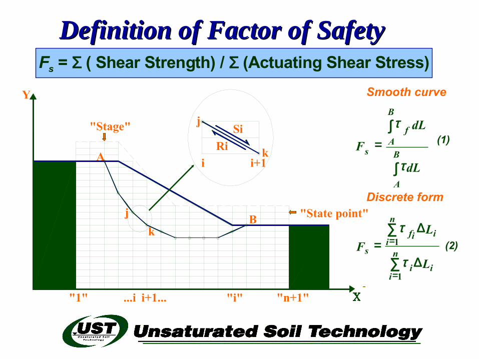
Definition of Factor of SafetyDefinition of Factor of Safety
Smooth curve
Discrete form
(1)
(2)
"Stage"
B "State point"
"n+1"
A
Y
"i""1"
Rii i+1
k
jSi
jk
...i i+1...
Fs = Σ ( Shear Strength) / Σ (Actuating Shear Stress)
∫
∫=
B
A
B
Af
s
dL
dL
Fτ
τ
∑
∑
=
=
∆
∆=
n
iii
n
iiif
sL
LF
1
1
τ
τ
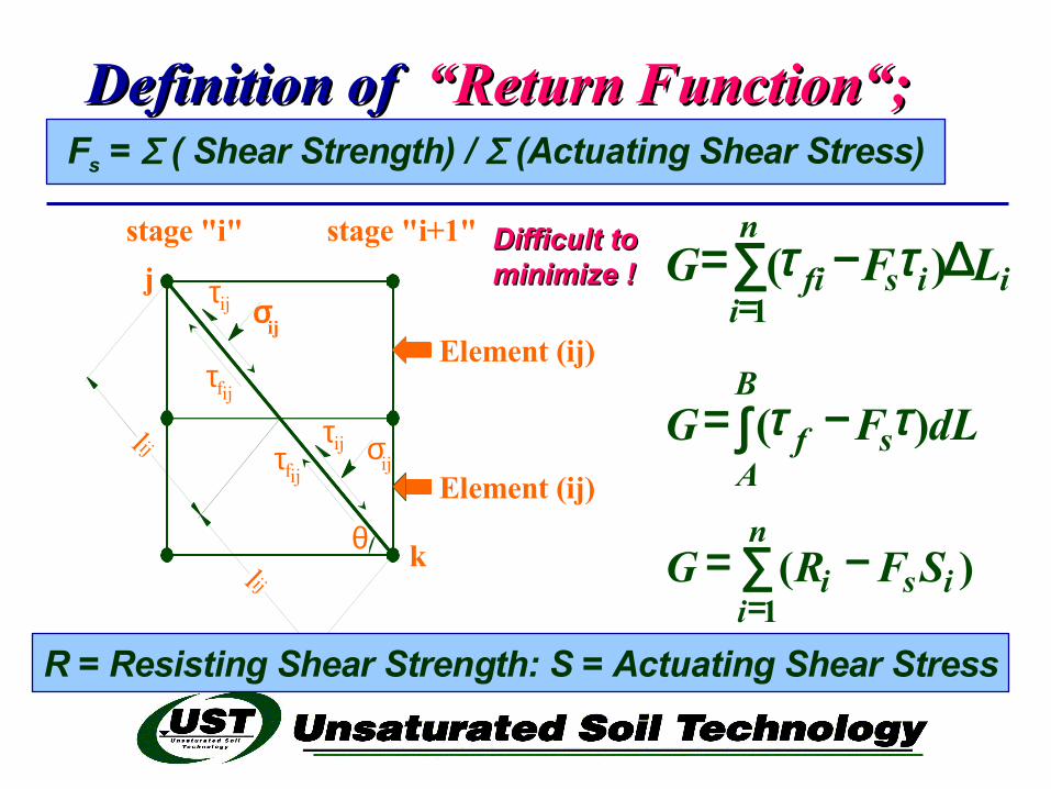
Definition of Definition of “Return Function“;“Return Function“; GG
stage "i+1"stage "i"
l ij
l ij
fτ
τfij
ij
jσijτ
ij
θ k
ijσijτ
Element (ij)
Element (ij)
R = Resisting Shear Strength: S = Actuating Shear Stress
Fs = Σ ( Shear Strength) / Σ (Actuating Shear Stress)
Difficult to Difficult to minimize !minimize ! ∑
=∆−=
n
iiisfi LFG
1)( ττ
dLFG sB
Af )( ττ −= ∫
∑=
−=n
iisi SFRG
1)(
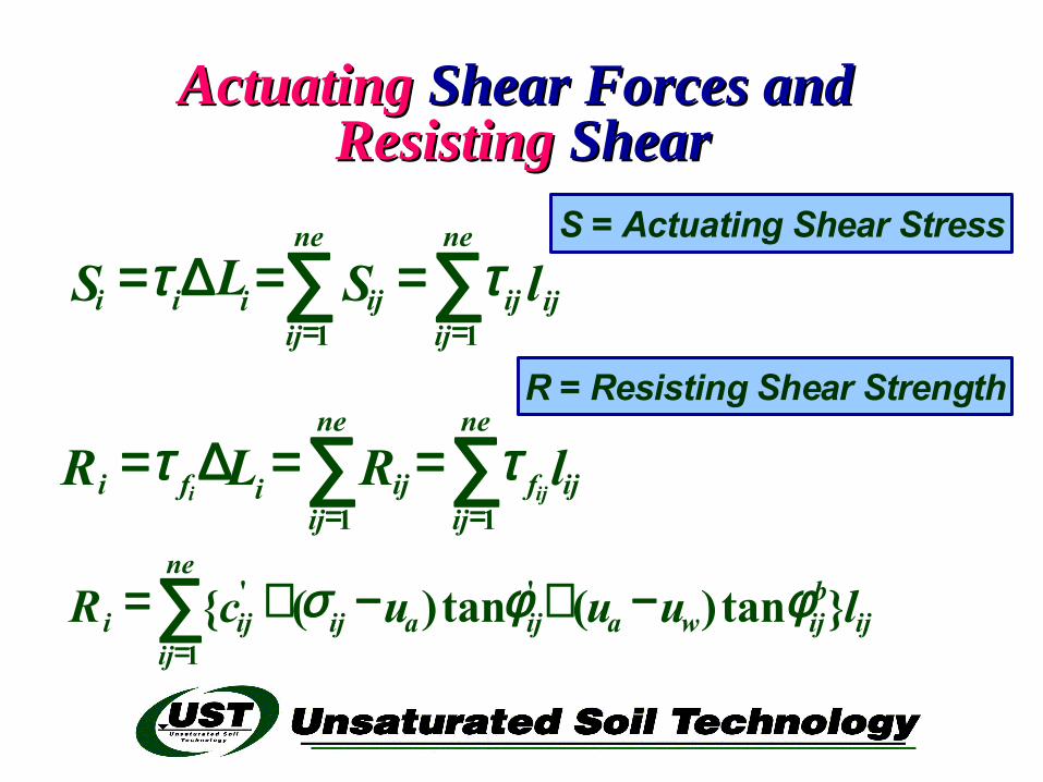
ActuatingActuating Shear Forces and Shear Forces and Resisting Resisting Shear Shear
S = Actuating Shear Stress
R = Resisting Shear Strength
∑∑==
==∆=ne
ijijij
ne
ijijiii l SLS
11
ττ
∑∑==
==∆=ne
ijijf
ne
ijijifi lRLR
iji11
ττ
ijbijwaijaij
ne
ijiji luuucR }tan)(tan)({ '
1
' φ φσ −+−+=∑=
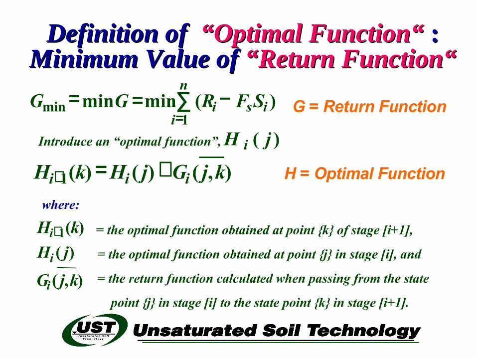
Definition of Definition of “Optimal Function““Optimal Function“ ::Minimum Value of Minimum Value of “Return Function““Return Function“
= the optimal function obtained at point {k} of stage [i+1],
= the optimal function obtained at point {j} in stage [i], and
= the return function calculated when passing from the state
point {j} in stage [i] to the state point {k} in stage [i+1].
where:
Introduce an “optimal function”,
H = Optimal Function
G = Return Function∑=
−==n
iisi SFRGG
1min )(minmin
)( jH i
),()()(1 kjGjHkH iii +=+
)(1 kHi+
)( jHi
),( kjGi
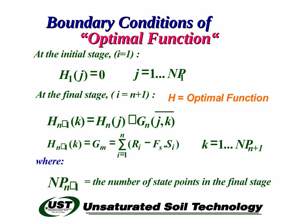
Boundary Conditions of Boundary Conditions of “Optimal Function““Optimal Function“
At the initial stage, (i=1) :
At the final stage, ( i = n+1) :
where:
= the number of state points in the final stage
H = Optimal Function
0)(1 =jH 1...1 NPj =
),()()(1 kjGjHkH nnn +=+
∑=
+ −==n
iisimn SFRGkH
11 ).()( ...1= n+1 NPk
1+nNP
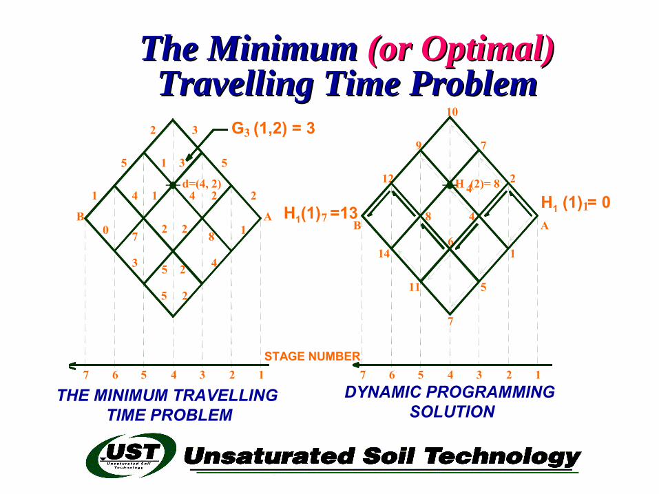
The Minimum The Minimum (or Optimal)(or Optimal) Travelling Time ProblemTravelling Time Problem
DYNAMIC PROGRAMMING SOLUTION
1
1
6
48
7
511
114
12
1H1 (1) = 0
9
2
7
4
7H1(1) =13A
H (2)= 8
123
10
B
567 4STAGE NUMBER
1234567
d=(4, 2)
3G (1,2) = 3
3
10
5 2
43 25
2 827
22441
55
32
B A
THE MINIMUM TRAVELLING TIME PROBLEM
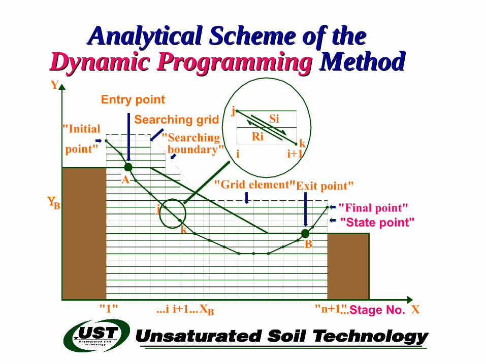
Analytical Scheme of the Analytical Scheme of the Dynamic ProgrammingDynamic Programming Method Method
Entry point
"1"
"Initial
A
B
point"
Y
"State point"
...i i+1...XB
B
"n+1" X...Stage No.
"Exit point"
Si
"Grid element"
boundary""Searching
i i+1k
Searching gridj
Ri
"Final point"j
k
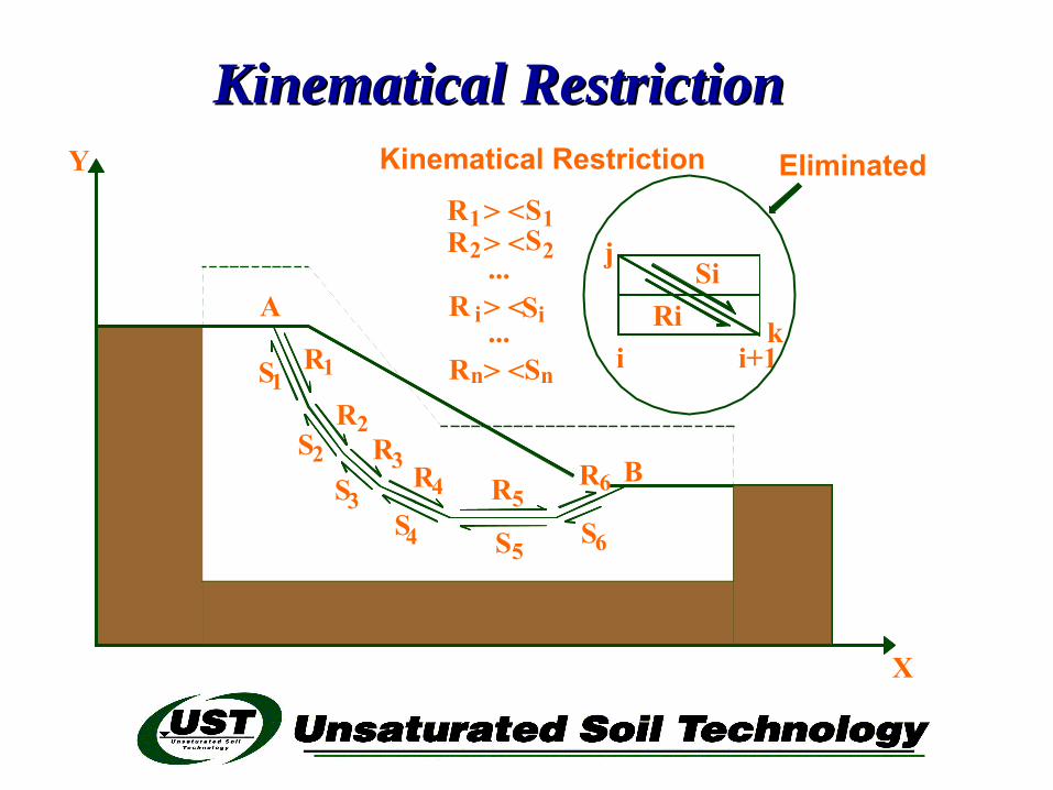
Kinematical RestrictionKinematical Restriction
5S 6
R
S R3
SR5
4
4RS2
23 BR6
S
RS1 1
A
X
Y
R1 1SR 22 S
i SiR
R nSn
...
...
Kinematical Restriction
Rii i+1
k
jSi
Eliminated> <> <
> <
> <
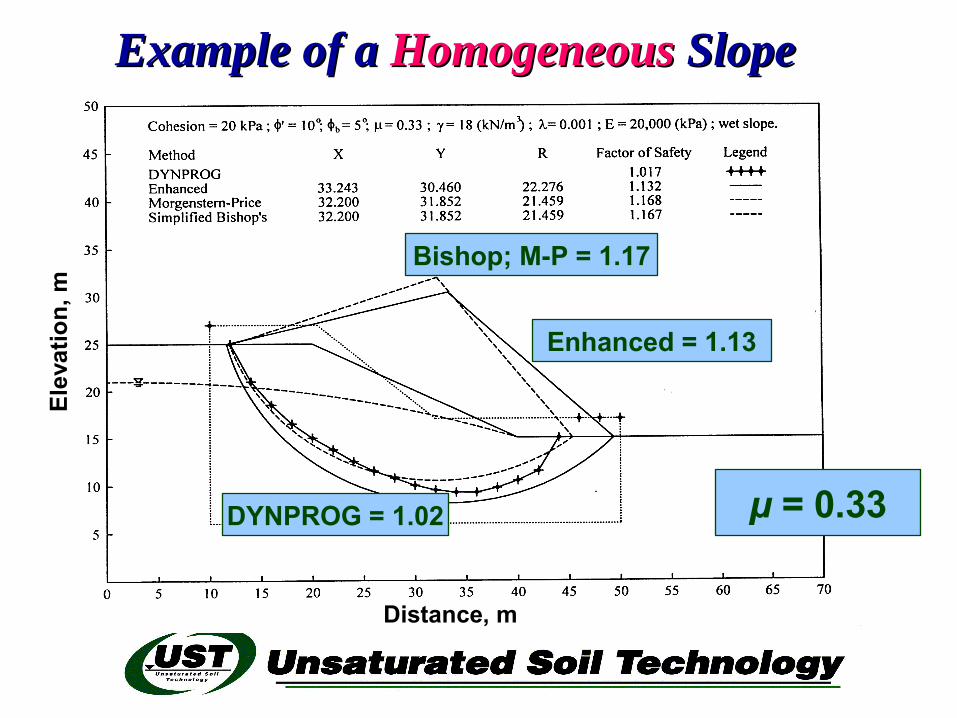
μ = 0.33DYNPROG = 1.02
Enhanced = 1.13
Bishop; M-P = 1.17
Distance, m
Elev
atio
n, m
Example of a Example of a Homogeneous Homogeneous SlopeSlope
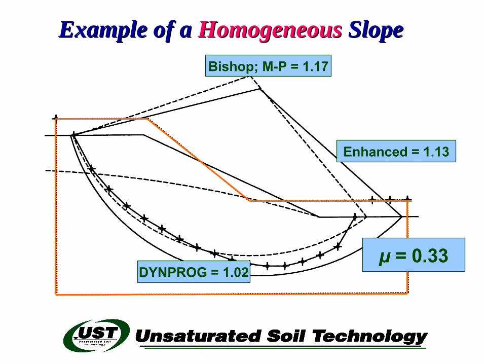
Example of a Example of a HomogeneousHomogeneous Slope Slope
μ = 0.33DYNPROG = 1.02
Bishop; M-P = 1.17
Enhanced = 1.13
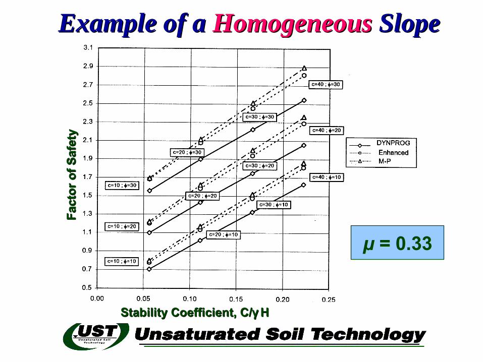
Example of a Example of a Homogeneous Homogeneous SlopeSlope
μ = 0.33
Fact
or o
f Saf
ety
Fact
or o
f Saf
ety
Stability Coefficient, C/Stability Coefficient, C/γ γ HH
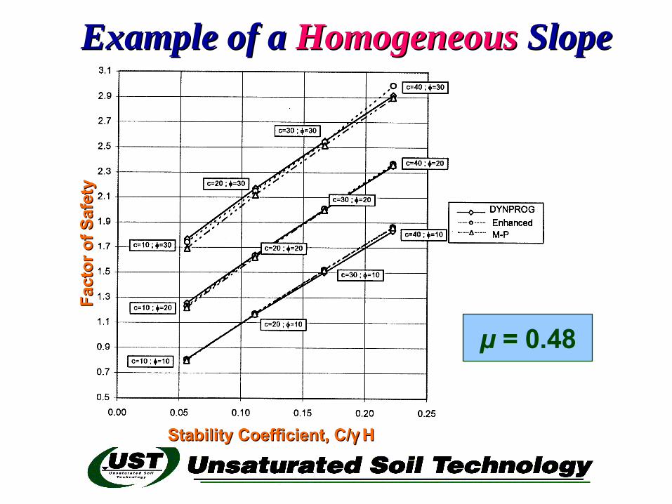
μ = 0.48
Fact
or o
f Saf
ety
Fact
or o
f Saf
ety
Stability Coefficient, C/Stability Coefficient, C/γ γ HH
Example of a Example of a Homogeneous Homogeneous SlopeSlope
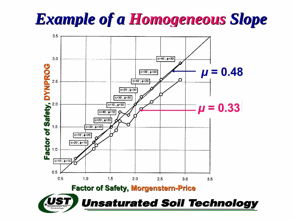
Example of a Example of a HomogeneousHomogeneous Slope Slope
μ = 0.33
μ = 0.48
Fact
or o
f Saf
ety,
Fact
or o
f Saf
ety,
DYN
PRO
GD
YNPR
OG
Factor of Safety,Factor of Safety, Morgenstern-PriceMorgenstern-Price
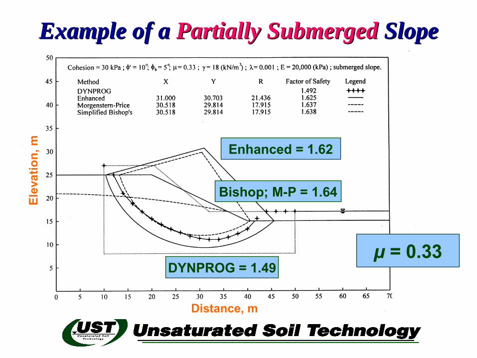
μ = 0.33
Distance, m
Elev
atio
n, m
Bishop; M-P = 1.64
Enhanced = 1.62
DYNPROG = 1.49
Example of a Example of a Partially SubmergedPartially Submerged Slope Slope
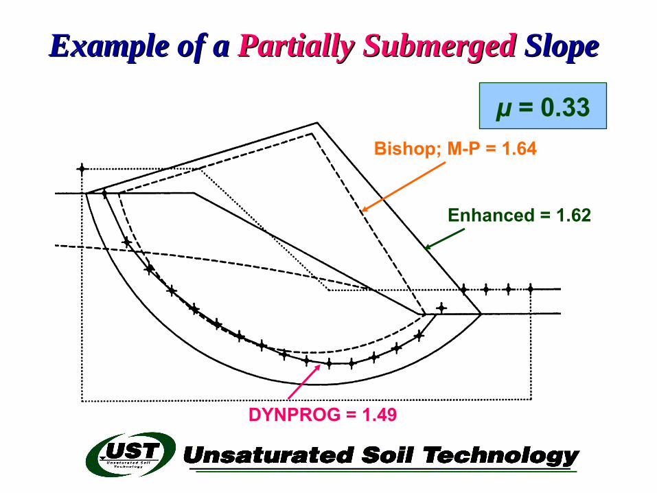
Example of a Example of a Partially SubmergedPartially Submerged Slope Slope
μ = 0.33
Enhanced = 1.62
Bishop; M-P = 1.64
DYNPROG = 1.49
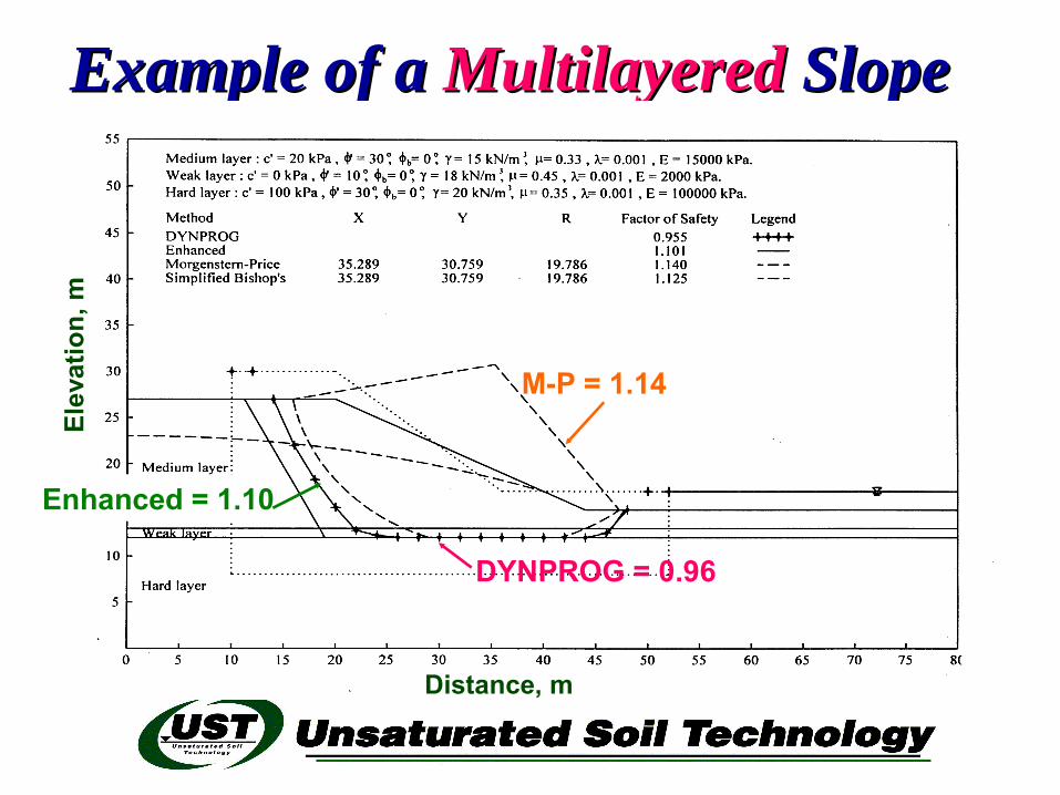
Example of a Example of a MultilayeredMultilayered Slope Slope
Enhanced = 1.10
M-P = 1.14
DYNPROG = 0.96
Distance, m
Elev
atio
n, m
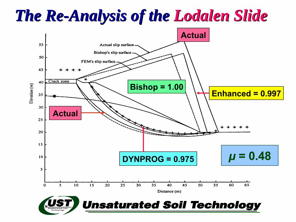
The Re-Analysis of the The Re-Analysis of the Lodalen SlideLodalen Slide
μ = 0.48DYNPROG = 0.975
Bishop = 1.00
Actual
Actual
Enhanced = 0.997
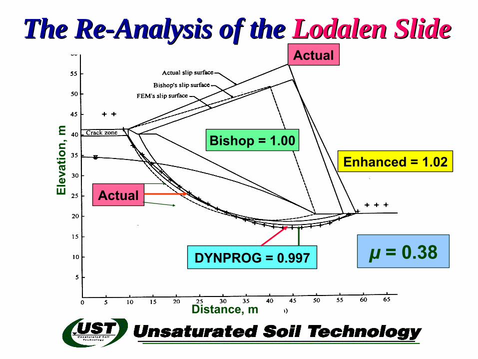
The Re-Analysis of the The Re-Analysis of the Lodalen SlideLodalen Slide
μ = 0.38
Enhanced = 1.02Bishop = 1.00
DYNPROG = 0.997
Actual
Distance, m
Elev
atio
n, m
Actual
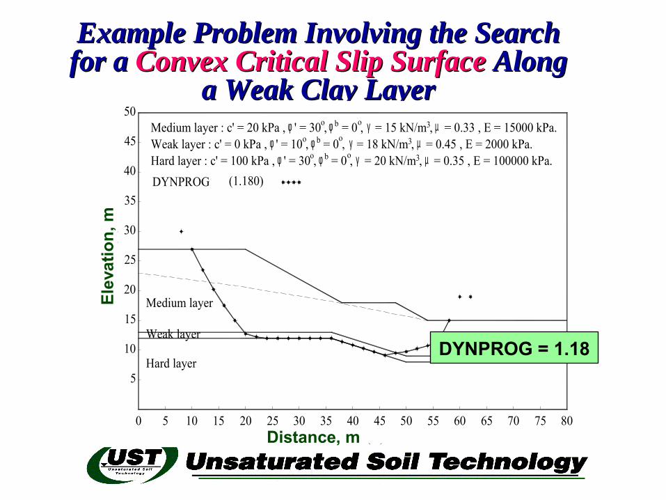
Example Problem Involving the Search Example Problem Involving the Search for a for a Convex Critical Slip SurfaceConvex Critical Slip Surface Along Along
a Weak Clay Layera Weak Clay Layer
40Distance (m)
150 5 10 20 25 30 35 45 50 6055 65 70 75 80
Medium layer20
10
5Hard layer
15Weak layer
Elev
ation
( m) 30
25
35
40
45
50
Hard layer : c' = 100 kPa , ' = 30 , = 0 , = 20 kN/m , = 0.35 , E = 100000 kPa.
Medium layer : c' = 20 kPa , ' = 30 , = 0 , = 15 kN/m , = 0.33 , E = 15000 kPa.Weak layer : c' = 0 kPa , ' = 10 , = 0 , = 18 kN/m , = 0.45 , E = 2000 kPa.
DYNPROG
φoφφ
(1.180)φ
φo bφ
o b
o γb
γγ
o
oµ3
3 µµ3
DYNPROG = 1.18
Distance, m
Elev
atio
n, m
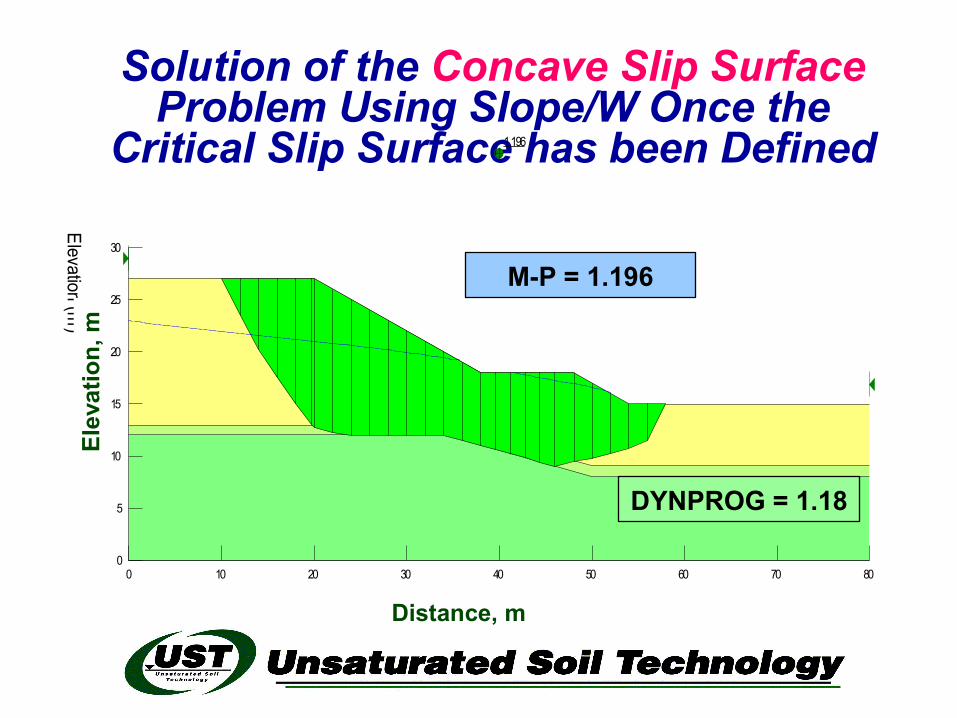
Solution of the Concave Slip Surface Problem Using Slope/W Once the
Critical Slip Surface has been Defined1.196
Distance (m)0 10 20 30 40 50 60 70 80
Elevation (m)
0
5
10
15
20
25
30
Elev
atio
n, m
Distance, m
M-P = 1.196
DYNPROG = 1.18
Conclusions from Conclusions from Step 2Step 2 Forward Forward The Shape of the critical slip surface can
be made part of the solution The critical slip surface can be irregular
in shape but must be kinematically admissible
No assumptions is required regarding the Location of the critical slip surface which is defined as an assemblage of linear segments
Force and moment equilibrium equations are satisfied through the stress analysis

Recommendations for the FutureRecommendations for the Future The normal and shear stresses should be The normal and shear stresses should be
studied using studied using more sophisticated stress-more sophisticated stress-strain nonlinear and elasto-plastic modelsstrain nonlinear and elasto-plastic models including Poisson‘s ratio effectsincluding Poisson‘s ratio effects
Study of Study of “true““true“ 3-dimensional modelling 3-dimensional modelling of slopes and past Case Historiesof slopes and past Case Histories
Dynamic Programming should be applied Dynamic Programming should be applied to to Lateral Earth PressureLateral Earth Pressure and and Bearing Bearing CapacityCapacity problems problems
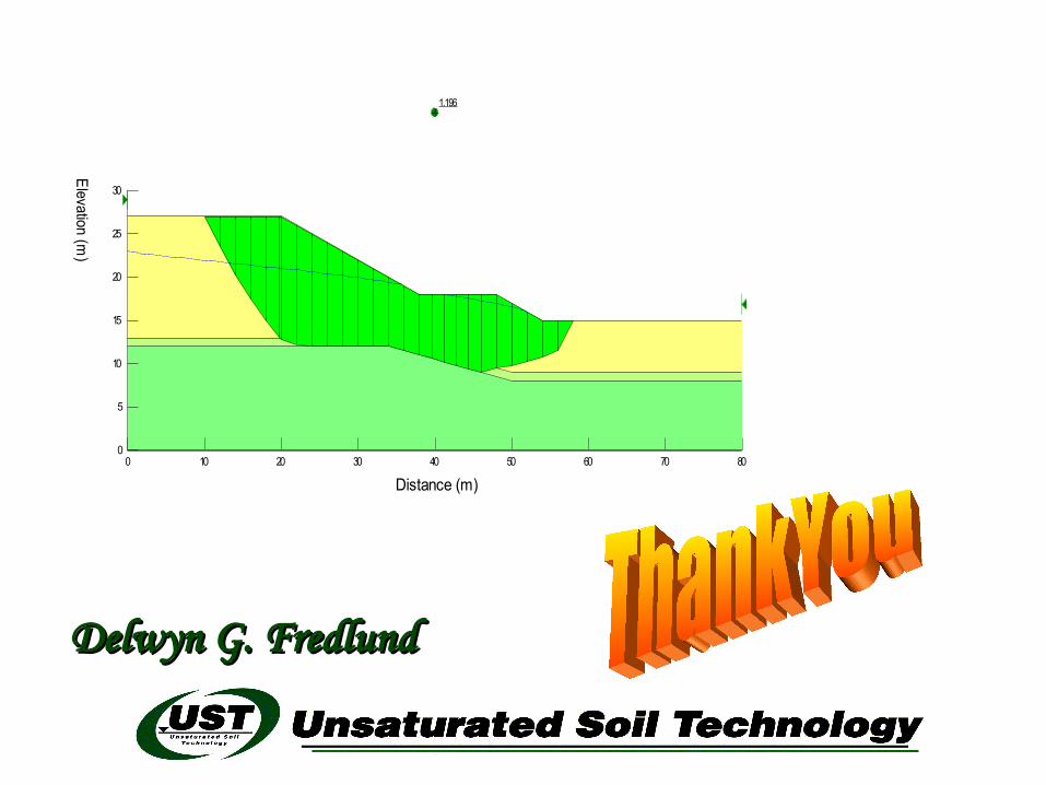
Delwyn G. FredlundDelwyn G. Fredlund
1.196
Distance (m)0 10 20 30 40 50 60 70 80
Elevation (m)
0
5
10
15
20
25
30