United States Department of Agriculture

Forest Service

Southern Research Station

Research Paper SRS-? 0

White Pine Site Index for the Southern Forest Survey

Bernard R. Parresol and John S. Vissage

White Pine Site Index for the Southern Forest Survey

Bernard R. Parresol and John S. Vissage

Abstract Table 14econd-growth white pine age-height data a

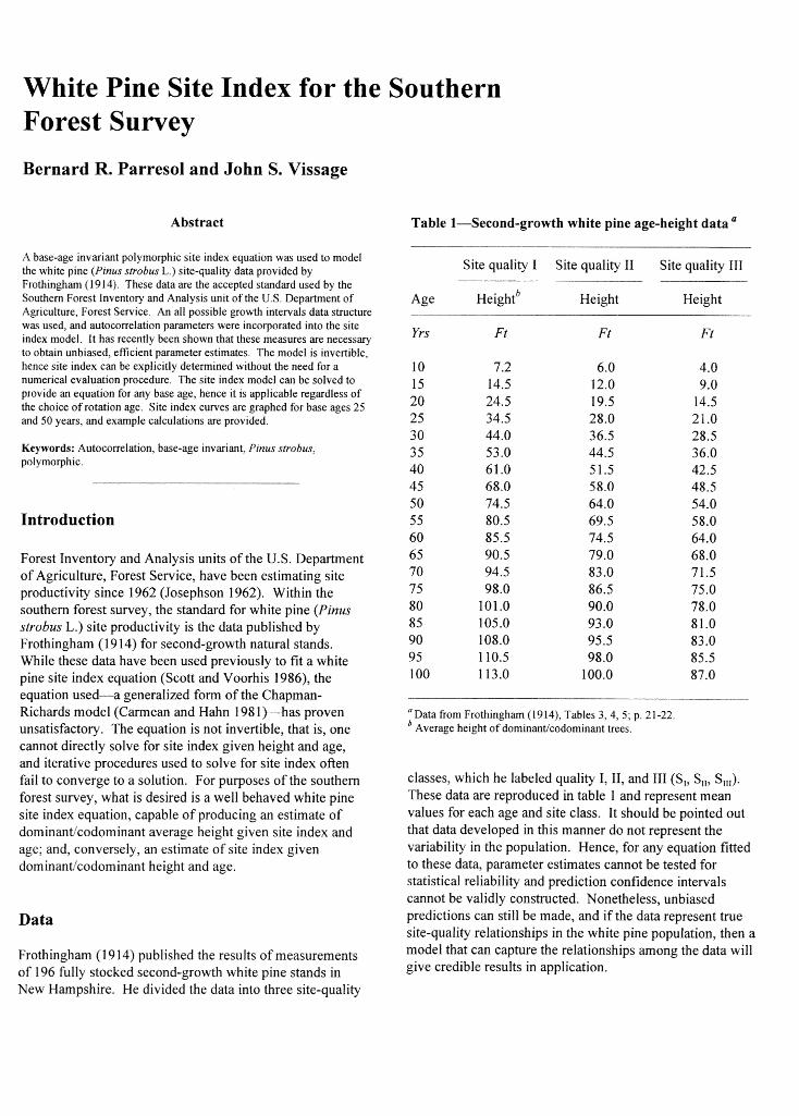
A base-age invariant polymorphic site index equation was used to model the white pine (Pznus strobus L.) site-quality data provided by Frothingham (1914). These data are the accepted standard used by the Southern Forest Inventory and Analysis unit of the U.S. Department of Agriculture, Forest Service. An all possible growth intervals data structure was used, and autocorrelation parameters were incorporated into the site index model. It has recently been shown that these measures are necessary to obtain unbiased, efficient parameter estimates. The model is invertible, hence site index can be explicitly determined without the need for a numerical evaluation procedure. The site index model can be solved to provide an equation for any base age, hence it is applicable regardless of the choice of rotation age. Site index curves are graphed for base ages 25 and 50 years, and example calculations are provided.

Keywords: Autocorrelation, base-age invariant, Pinus strobus, polymorphic.

Introduction

Forest Inventory and Analysis units of the U.S. Department of Agriculture, Forest Service, have been estimating site productivity since 1962 (Josephson 1962). Within the southern forest survey, the standard for white pine (Pinus strobus L.) site productivity is the data published by Frothingham (1 9 14) for second-growth natural stands. While these data have been used previously to fit a white pine site index equation (Scott and Voorhis 1986), the equation used-a generalized form of the Chapman- Richards model (Carmean and Hahn 198 1 )---has proven unsatisfactory. The equation is not invertible, that is, one cannot directly solve for site index given height and age, and iterative procedures used to solve for site index often fail to converge to a solution. For purposes of the southern forest survey, what is desired is a well behaved white pine site index equation, capable of producing an estimate of dorninanticodominant average height given site index and age; and, conversely, an estimate of site index given dorninanticodominant height and age.

Data

Frothingham (1 9 14) published the results of measurements of 196 fully stocked second-growth white pine stands in New Hampshire. He divided the data into three site-quality

Site quality I Site quality I1 Site quality I11

Height6 Height Height

Yrs

10 15 20 25 30 35 40 45 50 55 60

" Data from Frothingham (19 14), Tables 3,4, 5; p. 2 1-22. Average height of dominantlcodominant trees.

classes, which he labeled quality I, 11, and I11 (S,, S,,, S,,,). These data are reproduced in table 1 and represent mean values for each age and site class. It should be pointed out that data developed in this manner do not represent the variability in the population. Hence, for any equation fitted to these data, parameter estimates cannot be tested for statistical reliability and prediction confidence intervals cannot be validly constructed. Nonetheless, unbiased predictions can still be made, and if the data represent true site-quality relationships in the white pine population, then a model that can capture the relationships among the data will give credible results in application.

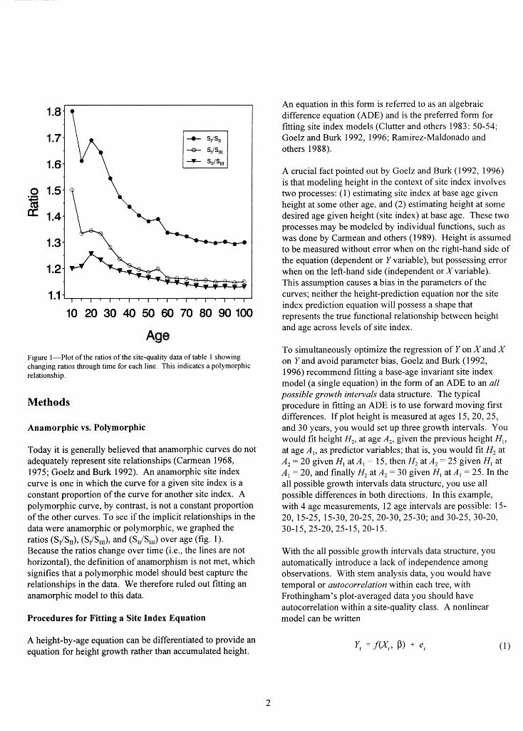
Figure l-Plot of the ratios of the site-quality data of table 1 showing changing ratios through time for each line. This indicates a polymorphic relationship.

Methods

Anamorphic vs. Polymorphic

Today it is generally believed that anamorphic curves do not adequately represent site relationships (Carmean 1968, 1975; Goelz and Burk 1992). An anamorphic site index curve is one in which the curve for a given site index is a constant proportion of the curve for another site index. A polymorphic curve, by contrast, is not a constant proportion of the other curves. To see if the implicit relationships in the data were anamorphic or polymorphic, we graphed the ratios (S,IS,,), (S,IS,,,), and (S,,/S,,,) over age (fig. 1). Because the ratios change over time (i.e., the lines are not horizontal), the definition of anamorphism is not met, which signifies that a polymorphic model should best capture the relationships in the data. We therefore ruled out fitting an anamorphic model to this data.

Procedures for Fitting a Site Index Equation

A height-by-age equation can be differentiated to provide an equation for height growth rather than accumulated height.

An equation in this form is referred to as an algebraic difference equation (ADE) and is the preferred forrn for fitting site index models (Clutter and others 1983: 50-54; Goelz and Burk 1992, 1996; Ramirez-Maldonado and others 1988).

A crucial fact pointed out by Goelz and Burk (1 992, 1996) is that modeling height in the context of site index involves two processes: (1) estimating site index at base age given height at some other age, and (2) estimating height at some desired age given height (site index) at base age. These two processes may be modeled by individual functions, such as was done by Carmean and others (1989). Height is assumed to be measured without error when on the right-hand side of the equation (dependent or Y variable), but possessing error when on the left-hand side (independent or X variable). This assumption causes a bias in the parameters of the curves; neither the height-prediction equation nor the site index prediction equation will possess a shape that represents the true functional relationship between height and age across levels of site index.

To simultaneously optimize the regression of Yon X and X on Y and avoid parameter bias, Goelz and Burk (1 992, 1996) recommend fitting a base-age invariant site index model (a single equation) in the form of an ADE to an all possible growth intervals data structure. The typical procedure in fitting an ADE is to use forward moving first differences. If plot height is measured at ages 15,20,25, and 30 years, you would set up three growth intervals. You would fit height Hz, at age A,, given the previous height HI, at age A,, as predictor variables; that is, you would fit Hz at A, = 20 given HI at Al = 15, then H, at A, = 25 given HI at A l = 20, and finally H, at A, = 30 given H, at A , = 25. In the all possible growth intervals data structure, you use all possible differences in both directions. In this example, with 4 age measurements, 12 age intervals are possible: 15- 20, 15-25, 15-30,20-25,20-30,25-30; and 30-25, 30-20, 30-15,25-20,25-15,20-15.

With the all possible growth intervals data structure, you automatically introduce a lack of independence among observations. With stem analysis data, you would have temporal or autocorrelation within each tree, with Frothinghm7s plot-averaged data you should have autocorrelation within a site-quality class. A nonlinear model can be written

where Model

the error terms are assumed to be independent and identically distributed.

A number of researchers have pointed to desirable attributes for site index equations (e.g., Bailey and Clutter 1974,

Under nonindependence, the nomal procedure is to expand Goelz and Burk 1992, Scott and Voorhis 1986). The most frequently listed criteria are: (1) polymorphism, (2) sigmoid the error term to allow f~st-order autocorrelation: (S-shaped) growth pattern, (3) asymptote is a function of

where

the ei are now independent and identically distributed.

Goelz and Burk (1992) point out that when using all possible growth intervals, the model is more complex:

where

Y,j depicts prediction of height i by using Y, (height j), X, (age i), a n d 4 (age j .c- i) as predictor variables.

Consequently, the error term must be further expanded:

+ E , , e. , = j + ye,, j -1 II IJ

site index (increases with increasing site index), and

(2) (4) logical behavior (height should be zero at age zero and equal to site index at base age). With these criteria in mind, we examined a variety of models, selected several to fit to the data, and finally settled on one described by Clutter and Jones (1 980). The function, in ADE format, is

Equation (4) represents the autocorrelation structure inherent in fitting site index models to an all possible growth intervals data structure. The parameter p accounts for the autocorrelation between the current residual and the residual from estimating Y,-, using as a predictor. The y parameter accounts for the autoconelation between the current residual and the residual from estimating Y, using Y,-! as a predictor variable. Goelz and Burk (1 992, 1996), as well as many other modelers (e.g., Parresol 1993), also recommend correcting for heteroscedasticity.

A final point to be noted is that when using the all possible growh intervals data structure, standard errors for the parameter estimates will be too small, because the number of observations are artificially inflated. Goelz and Burk (1996) give a simple correction factor. Because we will not be constructing confidence intervals, we are not concerned with this point (for this application). In summary, to fit site index models one should (1) use an ADE form, (2) use all possible growth intervals, (3) account for autocorrelation and heteroscedasticity, and (4) inflate standard errors.

1 1.4 = ..P[P~(; - ;)I ( l n q - P2- A , + P,)

(5)

where

ln stands for natural logarithms, H , and A, represent the predictor height and age, 4 is the predicted height at age A,, the p's are model parameters, and e is stochastic error.

This function meets most of the above criteria and, in addition, has the benefit of being base-age invariant. Base- age invariant curves are more general than base-age-specific equations, because they can predict height at any age given height at any other age. This function behaves very well for ages 10 and greater, giving small values then increasing in a sigmoid pattern to the asymptote value, which increases with increasing site index.

To use model (5) to estimate average stand height (H) for some desired age (A), given site index (S) and its associated base age (A,), simply substitute S for I-i, and A, for A ,:

Similarly, to estimate site index at some chosen base age, given stand height and age, simply substitute S for H2 and A, for A, in model (5):

Application

Generally, the correlation parmeters can be ignored when using equations (6) and (7) for predicting height and site index. The quantities e ,-,,, and e ,,,, will probably not be known unless one is working repeatedly on the same plot, in which case they could be determined and utilized to predict a future value. Our main purpose in using the autocorrelation error structure was to obtain unbiased, efficient estimates of the P vector.

Results Base Age 25 System

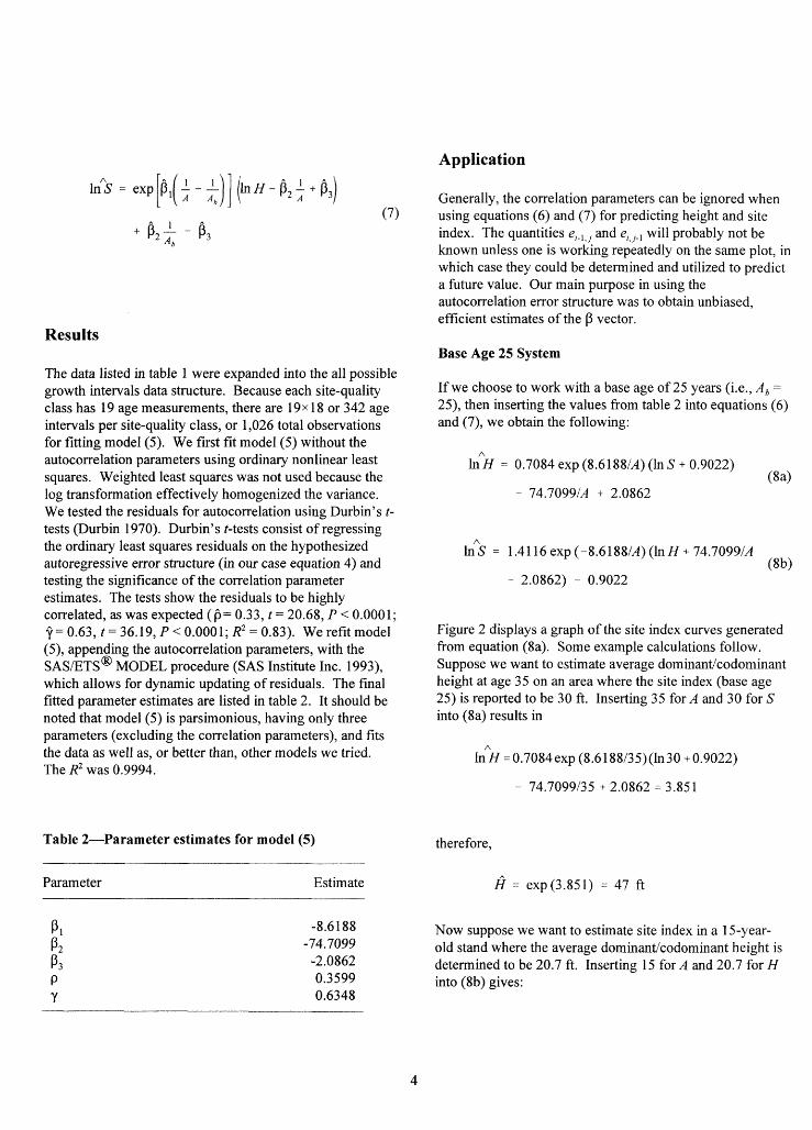
The data listed in table 1 were expanded into the all possible growth intervals data structure. Because each site-quality class has 19 age measurements, there are 19x 18 or 342 age intervals per site-quality class, or 1,026 total observations for fitting model (5). We first fit model (5) without the autocorrelation parameters using ordinary nonlinear least squares. Weighted least squares was not used because the log transformation effectively homogenized the variance. We tested the residuals for autocorrelation using Durbin's t- tests (Durbin 1970). Durbin's t-tests consist of regressing the ordinary least squares residuals on the hypothesized autoregressive error structure (in our case equation 4) and testing the significance of the correlation parameter estimates. The tests show the residuals to be highly correlated, as was expected ( l j = 0.33, t = 20.68, P < 0.0001; f = 0.63, t = 36.19, P < 0.0001; R2 = 0.83). We refit model (5), appending the autocorrelation parameters, with the SASIETS@ MODEL procedure (SAS Institute Inc. 1993), which allows for dynamic updating of residuals. The final fitted parameter estimates are listed in table 2. It should be noted that model (5) is parsimonious, having only three parameters (excluding the correlation parameters), and fits the data as well as, or better than, other models we tried. The R2 was 0.9994.

Table 2-Parameter estimates for model (5)

If we choose to work with a base age of 25 years (i.e., A, =

25), then inserting the values from table 2 into equations (6) and (7), we obtain the following:

lnhH = 0.7084 exp (8.6188iA) (1nS + 0.9022) (8a)

lnAs = 1.41 16 exp (-8.6188IA) (In H + 74.70991A (8b)

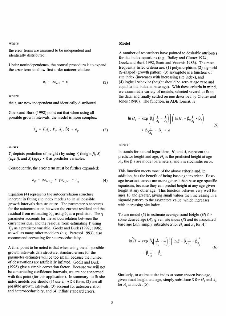
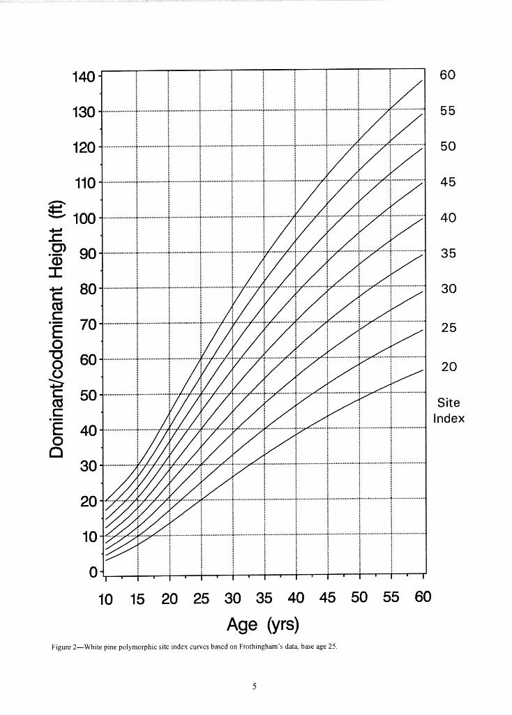
Figure 2 displays a graph of the site index curves generated from equation (8a). Some example calculations follow. Suppose we want to estimate average dominantlcodominant height at age 35 on an area where the site index (base age 25) is reported to be 30 ft. Inserting 35 for A and 30 for S into (8a) results in

therefore,

Parameter Estimate I? = exp(3.851) = 47 ft

-8.6188 Now suppose we want to estimate site index in a 15-year- -74.7099 old stand where the average dominantlcodominant height is

-2.0862 determined to be 20.7 ft. Inserting 15 for A and 20.7 for H 0.3599 into (8b) gives: 0.6348

Site Index

Figure 2-White pine polymorphic site index curves based on Frothingham's data, base age 25.

therefore,

Now suppose we want to estimate site index in a 35-year- old stand where the average do~nantfcodominant height is determined to be 52.6 ft. Inserting 35 for A and 52.6 for H into (9b) gives:

l h = 1 .I881 exp (-8.6188135)(1n52.6

+ 74.7099135 2.0862) + 0.5920 = 4.317

S ̂ = exp (3.806) = 45 ft

therefore,

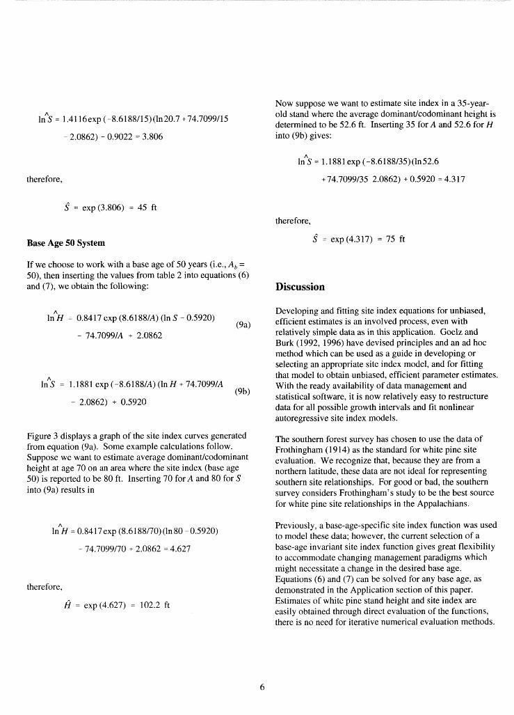
Base Age 50 System S ̂ = exp (4.317) = 75 ft

If we choose to work with a base age of 50 years (is., A, = 50), then inserting the values from table 2 into equations (6) and (7), we obtain the following: Discussion

Developing and fitting site index equations for unbiased, 1;H = 0.8417 exp (8.6188/A) (In S - 0.5920)

(9,) efficient estimates is an involved process, even with

- 74.70991A + 2.0862 relatively simple data as in this application. Goelz and Burk (1 992, 1996) have devised principles and an ad hoc method which can be used as a guide in developing or selecting an appropriate site index model, and for fitting that model to obtain unbiased, efficient parameter estimates.

ln?' = 1.1881 exp (-8.6188/A) (1nH + 74.7099/A With the ready availability of data management and

- 2.0862) + 0.5920 (9b) statistical software, it is now relatively easy to restructure

data for all possible growth intervals and fit nonlinear autoregressive site index models.

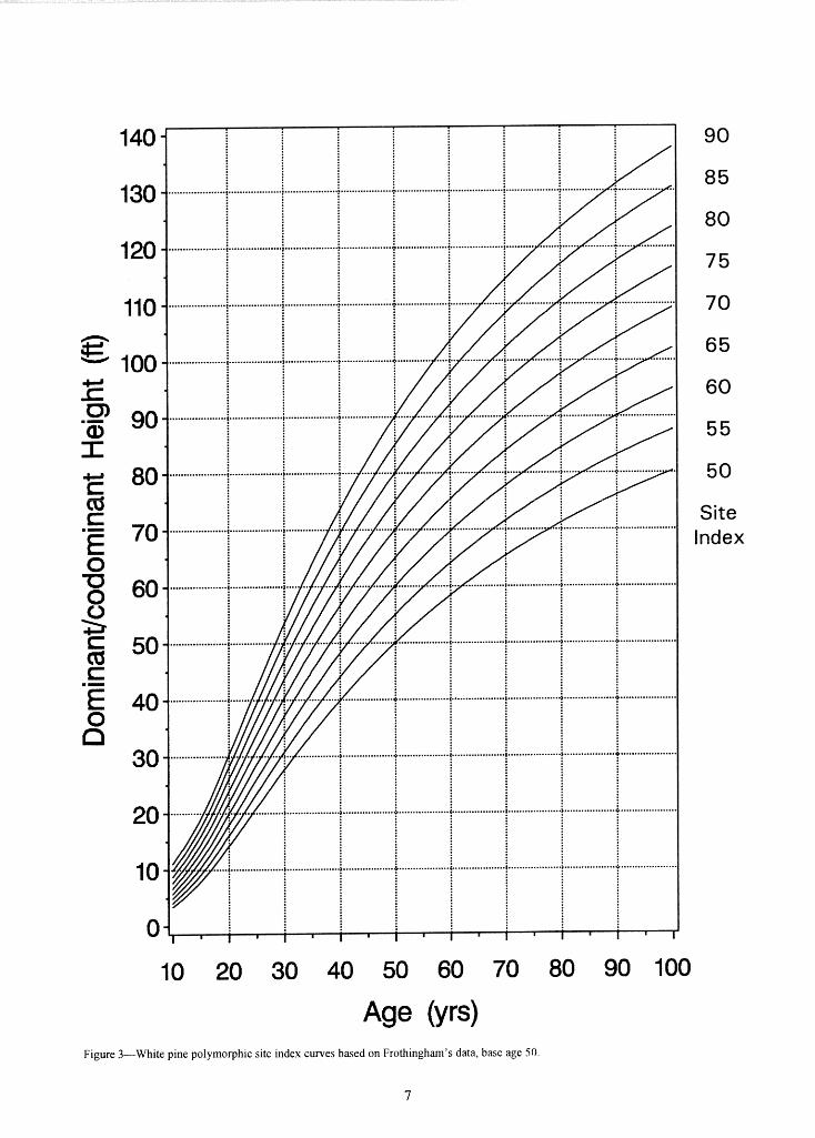
Figure 3 displays a graph of the site index curves generated The southern forest survey has chosen to use the data of from equation (9a). Some example calculations follow. Frothingham (1914) as the standard for white pine site Suppose we want to estimate average dominant/codominant evaluation. We recognize that, because they are from a height at age 70 on an area where the site index (base age northern latitude, these data are not ideal for representing 50) is reported to be 80 ft. Inserting 70 for A and 80 for S southern site relationships. For good or bad, the southern into (9a) results in survey considers Frothingham's study to be the best source

for white pine site relationships in the Appalachians.

I& = 0.84 17 exp (8.61 88/70) (1n 80 - 0.5920)

- '74.7099170 + 2.0862 = 4.627

therefore,

I? = exp (4.627) = 102.2 ft

Previously, a base-age-specific site index function was used to model these data; however, the current selection of a base-age invariant site index function gives great flexibility to accommodate changing management paradigms which might necessitate a change in the desired base age. Equations (6) and (7) can be solved for any base age, as demonstrated in the Application section of this paper. Estimates of white pine stand height and site index are easily obtained through direct evaluation of the functions, there is no need for iterative numerical evaluation methods.

n

loo

10 20 30 40 50 60 70 80 90 100

Age (Y rs) Figure 3-White pine polymorphic site index curves based on Frothingham's data, base age 50.

Site Index

Acknowledgments

The authors thmk Dr. Robert M. Farrar, Jr., retired project leader from the Southem Research Station now living in Mississippi, and Dr. Jeffery G. Goelz with the Southern Hardwoods Laboratory of the Southern Research Station, Stoneville, MS, for their reviews and advice. The authors would also like to thank the three anonymous reviewers for their helpfbl comments and suggestions.

Literature Cited

Bailey, R.L.; Clutter, J.L. 1974. Base-age invariant polymorphic site curves. Forest Science. 20: 155-1 59.

Carmean, W.H. 1968. Tree height growth patterns in relation to soil and site. In: Proceedings of the third North American forest soils conference: tree growth and forest soils. Corvalis, OR: Oregon State University Press: 499-5 12.

Carmean, W.H. 1975. Forest site quality evaluation in the United States. Advances in Agronomy. 27: 209-269.

Carmean, W.H.; Hahn, J.T. 1981. Revised site index curves for balsam fir and white spruce in the Lake States. Res. Note NC-269. St. Paul, IvlN: U.S. Department of Agriculture, Forest Service, North Central Forest Experiment Station. 4 p.

Carmean, W.H.; Hahn, J.T.; Jacobs, R.D. 1989. Site index curves for forest tree species in the eastern United States. Gen. Tech. Rep. NC-128. St. Paul, MN: U.S. Department of Agriculture, Forest Service, North Central Forest Experiment Station. 142 p.

Clutter, J.L.; Jones, E.P., Jr. 1980. Prediction of growth after thinning in old-field slash pine plantations. Res. Pap. SE-217. Asheville, NC: U.S. Department of Agriculture, Forest Service, southeastern Forest Experiment Station. 14 p.

Clutter, J.L.; Fortson, J.C.; Pienaar, L.V.; Brister, G.H.; Bailey, R.L. 1983. Timber management: a quantitative approach. New York: John Wiley & Sons. 333 p.

Durbin, J. 1970. Testing for serial correlation in least-squares regression when some of the regressors are lagged dependent variables. Econometrics. 50: 4 1042 1.

Frothingham, E.H. 1914. White pine under forest mmagement. Bull. 13. Washington, DC: U.S. Department of Agriculture. 70 p.

Goelz, J.C.G.; Burk, T.E. 1992. Development of a well behaved site index equation: jack pine in north central Ontario. Canadian Journal of Forest Research. 22: 776-784.

Goelz, J.C.G.; Burk, T.E. 1996. Measurement error causes bias in site index equations. Canadian Journal of Forest Research. 26: 1585-1 593.

Josephson, H.R. 1962. Forest Survey. Washington, DC: U.S. Department of Agriculture. Forest Service, Interagency Memorandum, November 16, 1962. 53 p.

Parresol, B.R. 1993. Modeling multiplicative error variance: an example predicting tree diameter from stump dimensions in baldcypress. Forest Science. 39: 670-679.

Ramirez-Maldonado, H.; Bailey, R.L.; Borders, B.E. 1988. Some implications of the algebraic difference approach for developing growth models. In: Ek, A.R.; Shifley, S.R.; Burk, T.E. eds. Proceedings IUFRO conference on forest growth modeling and prediction, 1987 August 23- 27; Minneapolis, MN. Gen. Tech. Rep. NC-120. St. Paul, MI?: U.S. Department of Agriculture, Forest Service, North Central Forest Experiment Station: 73 1-738.

SAS Institute Inc. 1993. SAS/ETS@ user's guide, version 6,2d ed. Cary, NC: SAS Institute Inc. 1,022 p.

Scott, C.T.; Voorhis, N.G. 1986. Northeastern forest survey site index equations and site productivity classes. Northern Journal of Applied Forestry. 3: 144-148.

Parresol, Bernard R.; Vissage, John S. 1998. White pine site index for the southern forest survey. Res. Pap. SRS-10. Asheville, NC: U.S. Department of Agriculture, Forest Service, Southern Research Station. 8 p.

A base-age invariant polymorphic site index equation was used to model the white pine (Pinus strobus L.) site-quality data provided by Frothingham (1914). These data are the accepted standard used by the Southern Forest Inventory and Analysis unit of the U.S. Department of Agriculture, Forest Service. An all possible growth intervals data structure was used, and autocorrelation parameters were incorporated into the site index model. It has recently been shown that these measures are necessary to obtain unbiased, efficient parameter estimates. The model is invertible, hence site index can be explicitly determined without the need for a numerical evaluation procedure. The site index model can be solved to provide an equation for any base age, hence it is applicable regardless of the choice of rotation age. Site index curves are graphed for base ages 25 and 50 years, and example calculations are provided.

Keywords: Autocorrelation, base-age invariant, Pinus strohus, polymorphic.