Who has the power in the EU?∗

Jason Barr†and Francesco Passarelli‡

December 13, 2004

Abstract

The European Union (EU) is facing the challenge of enlargement toalmost double its size; which has strong implications for the balance ofpower among member states. Building on the work of Shapley (1977)and Owen (1972), we present a measure of power that is based onplayers’ preferences and number of votes. We apply this measure tothe Council of Ministers to see who wields power now and who is likelyto wield power in the future. We also provide a rationale to explainwhy the negotiations for the new Constitution have been so difficult.Further, we show how a country’s power can change based on thepreferences of the agenda setter, which, in this case, is the EuropeanCommission.JEL Classification: C71, D72, D78, H11Keywords: Power Indices, European Union, Principal Components

∗The authors would like to thank Massimo Bordignon, Sandro Brusco, Mario Gilli,Manfred Holler, Annamaria Lusardi and Stefan Napel for their comments and suggestionson earlier drafts. Finally we appreciate the helpful discussions with Alberto Alesina, Pier-paolo Battigalli, Gérard Roland and Guido Tabellini. Any errors are the sole responsibilityof the authors.

†Rutgers University, Newark. Dept. of Economics, Newark, NJ 07102. email: jm-barr@andromeda.rutgers.edu.

‡Corresponding Author. University of Teramo and Bocconi University. email:francesco.passarelli@uni-bocconi.it

1

1 Introduction

The European Union (EU) is facing the challenge of an enlargement thathas almost doubled the number of members. As of May 1, 2004, ten newmembers have entered the Union; two potential member states are takingsteps towards full political and economic integration. The widespread beliefsare that the current institutional design is inadequate to face this challenge,and that the EU can no longer delay reforms that will give European decision-making mechanisms deeper democratic foundations and greater efficiency.At the heart of the debate is the problem of locating the optimal balance

between the intergovernmental nature of the Union, which is basically anagreement among sovereign member states, and the federal development ofthe EU. The attempt made by the Treaty of Nice (December 2000) to solvethis historical dichotomy, and, at the same time, to prepare the Union for theenlargement has failed primarily because the representatives of the nationalgovernments were reluctant to change the current institutional architecturethat grants more power to the member states (through the Council of Min-isters) than to the European Parliament (directly elected by the citizens)and to the European Commission (a centralized institution with power ofinitiative).Since the Laeken Summit (December 2001), the problem of institutional

reforms has been approached with a radically new method. A ConstitutionalConvention has been working on the enormous undertaking of constructinga decision-making system that remains efficient and meets the principlesof legitimacy and acceptability. After the intergovernmental negotiationsand adjustments, the Convention’s proposals were endorsed by the BruxellesSummit on June 18-19th 2004. On October 29, the heads of each the stateshave signed in Rome the Constitutional Treaty (CT). The constitutionalprocess will eventually be concluded with ratification by the member states.1

If the new institutional rules come into force, there will be a new Presidentfor the European Council, a Vice-President in charge of foreign affairs, a newCommission, a more powerful EU Parliament, and new voting schemes forthe Council of Ministers.The issue of decision making within the Council itself is quite important.

There is a broad consensus that even after the CT the Council will continue1Some countries will ratify the Constitutional Treaty only after referenda. This makes

the final outcome quite uncertain.

2

to have a prevailing role over the EU Parliament. The codecision procedure(i.e., the Parliament codecides issues with the Council) does not extend overall the policy issues, and in areas such as foreign policy and internal affairs theParliament plays a minor role. In addition, Napel and Widgrén (2003) usinga Nash bargaining rationale, show that a qualified majority in the Councilversus a simple majority in the Parliament gives the former more power thanthe latter, despite the codecision.2

In December 2003, the member states failed to reach an agreement onthe new Constitution because of the ”weighted vote” issue. Arguably, thecountries have been evaluating the losses and the gains from the new systemas compared to the Nice one. Initially, Spain and Poland have opposed theConvention’s proposal, saying that it will deeply modify the power distri-bution among the member states. Only after adjustments of the majoritythresholds did they accept the new CT, which ostensibly gives them morepower. The new voting scheme, which, if ratified, will come into effect in2009, will change the current rules of the bargaining among the nationalgovernments themselves, the different levels of government (within the coun-tries and between EU and country members) and the EU institutions. Inthis paper we focus on the game among the governments that takes placewithin the Council of Ministers.

1.1 Constitutional rules and European bargaining

Despite the relative narrowness of its budget, the EU has already acquireda wide set of competencies.3 The benefit from participating in the Unioncomes from the coordination and centralization of several policy areas, suchas a single currency, internal and external trade, competition, internationalrelations, and social protection. The literature on political economy, fromfiscal federalism to contract theory, offers contributions on what the EuropeanUnion should do and how it should be done (Alesina, et al., 2002, Alesinaand Perotti, 2004, Berglof, et al., 2003).The distribution of the EU surplus through negotiations and lobbying are

part of the daily life of the EU institutions. Part of this bargaining game

2Noury and Roland (2002) show that the coalitions within the European Parliamentfollow “party group” dynamics, rather than a “national” one.

3Almost 80% of the legislation issued by the member states emerges directly or indi-rectly from the application at the national level of the European law. The budget of theEU is limited to 1.27% of the aggregate GDP.

3

takes place at intergovernmental level: every Council meeting, including thepreparatory work, can be considered a non-cooperative game played by thedelegations of the states within the rules of the Treaty. However, in the con-stitutional phase of writing the Treaty, it is important to abstract away fromthe political interests present in particular voting environments and concen-trate on the rules of the game, and on their ability to generate equitabledistribution schemes.As such, this analysis can be conducted within the theoretical framework

of cooperative game theory. Thanks to the seminal work of Shapley andShubik (1954), the concept of the Shapley Value (Shapley, 1953) is taken asan index of the a priori power of the members in a committee. In summary,the Shapley-Shubik index is a measure of the relative frequency with which amember country can determine the outcome of a particular vote if all possiblecoalitions of a fixed number of member states were equally likely to occur;and it is, in general, some function of the number of votes and the majoritythreshold.4

Conventional wisdom holds that France and Germany, for example, arethe big “players” in the EU arena. This is simply true from an a priori con-sideration due to their having the largest number of votes and consequentlythe largest Shapley-Shubik indices. But why is the same power not conven-tionally assigned to Italy and United Kingdom, who have the same weightin the Council? Moreover and in general, how are the preferences of thecountries likely to affect outcomes? What will happen after enlargement?Here, we expand upon the definition and measurement of power as proposedby Shapley and Shubik. We discuss and estimate a spatial measure of theShapley Value, which comes directly from the preferences of the memberstates.

This paper is novel in several respects. First, from a theoretical point

4In our analyses, the Shapley-Shubik index (and Normalized Banhalf Index) turn outto be simple linear functions of the number of votes of the nations. For example, for the 15EU countries, with votes distributed according to the ’Pre-Nice’ scenario, we could predictthe Shapley Value from the votes by the simple OLS regression function:

∧SS = −0.002+

(0.0009)0.012(.0014)

V otes.

R2 = .998, n = 15. Standard Errors below estimates.

4

of view, we present a simple analytic extension of the work of Owen andShapley (1989). By directly incorporating the preferences of the players wegenerate a probabilistic-based power index that is easily calculated. Second,we extend this theory in a new direction by modelling the effect that anagenda-setter can have on the outcome of the game. The interaction of thepreferences of the players (e.g., the EU member countries) and the prefer-ences of the issue-setter (e.g., the EU Commission) can substantially alterthe power distribution among players. To the best of our knowledge, thisapproach has not been done elsewhere.From an empirical point of view this paper is new in the following ways.

First we directly measure the ’political preferences’ of the current and futureEU countries themselves. By analyzing EU-based polling data, we can geta measure of the extent to which member and potential-member countriesare relatively ’pro’ or ’con’ in regards to relinquishing decision making to theEU council. We then apply these measured preferences to computing powerindices for the EU countries. Finally, we measure how the distribution ofpower depends upon the preferences of the agenda setter.Our approach is sufficiently general to be applied to other federal contexts

or to political committees, where some information about the attitudes of themembers are available. Also applications to non-political institutions, suchas managerial boards or international organizations, could be envisaged.By directly using these preferences we find some interesting and novel

results:

• When considering the political positions of the countries, the numberof votes is not necessarily a good predictor of power. For example,decreasing the qualified majority threshold (from the current schemeto the CT) tends to shift the power to countries with moderate pref-erences. The Franco-German axis emerges from the centrality of theirpreferences and their size. Little power rests upon the Northern ’Eu-roskeptics’ or the Mediterranean ’Euroenthusiasts.’

• Under the system agreed at Nice, after the enlargement the leaderstend to lose most. Having a certain degree of Euroenthusiasm will putSpain, for example, in a favorable position. Euroenthusiasm will inturn favor of most newcomers. If the new Constitution does not comeinto force, the Eastern countries are likely to exercise a very strongpolitical influence on the Council, with a prominent role for the CzechRepublic.

5

• In comparing the Nice arrangement to the new Constitution, the Nicerules will allow the Eastern countries to collect almost 40% of totalpower, despite less than one fourth of population. The reapportionmentproposed by the CT favors moderate positions and restores the powerof the populous members, such as Germany and France. Spain emergesas a big player. The power shifts back to the Western members.

• A distorted pro-Europe Commission can cause the power to shift tocountries located on the Euroskeptic side of the political space. Thisshift tends to be more important when voters have less vague expecta-tions about the agenda setter’s preferences, when countries are highlydispersed on the political space, and when the majority threshold in-creases. The largest amount of power redistribution due to the agendasetter distortion occurs in the post-enlargement scenario with the Nicerules. The reallocation of power in favor of the large old members dueto the CT scenario is partially offset when the Commission is pro-EU.

1.2 Literature review

Although “power” in political science is a “penumbral” concept (Shapley,1977, p. 5), cooperative game theory has proved useful when investigatingthe influence that a voting system gives to the voters. Applications to theAmerican presidential election (Owen, 1975; Rabinowitz and MacDonald,1986) and to the Canadian constitutional reform (Kilgour, 1983) have gainedlegal importance in evaluating legislative reapportionments of votes.The literature on applications of power indices to the European Council

of Ministers is rich and widespread.5 This is partially due to the frequentenlargements of the EU, which provide new voting distributions to evaluate.This literature consists in computing or refining the standard Shapley-Shubikor Banzhaf (1965) indices for the EU members; thus, one usual assumption isthat the countries cannot be distinguished by their attitudes toward the EU.However, ignoring the “policy positions” of the European governments couldyield an overestimation of the power of the national governments with ex-treme preferences. Moreover, a priori power indices cannot take into accountthe“location” of the EU Commission, which plays the role of agenda-setterfor the Council.

5Holler and Owen (2001) and Felsenthal and Machover (1998) contain detailed refer-ences on the literature of power indices.

6

The theory of spatial indices can provide a strong analytical backgroundwhen ideological differences among players are crucial. Owen (1972) sug-gests a scheme of coalition formation that considers the ideological distancebetween voters in a political space. Building on Owen’s intuition, Shapley(1977) and Owen and Shapley (1989) provide a “non-symmetric” generaliza-tion of the Shapley-Shubik index in which each player’s power depends, inaddition to the voting rules, on her location in a political space.This generalized spatial index emphasizes the role of ideology in coalition

formation. In this scheme the coalitions are inspired by policy issues. Given apolicy issue, the players can be ordered by the level of support for that issue.The support defines the ordering within a coalition; only the “ideologicallyconsistent” orderings are considered. Thus the probability of a coalitionemerging is related to the number of policy issues it is inspired from.Shapley and Owen consider all the policy issues as equiprobable, assuming

the absence of any information about the issue generating mechanisms. Weargue that in the presence of an agenda setter some policy issues can bemore likely than others. As a consequence, ceteris paribus, the countrieswhich tend to be in pivotal positions in policy areas preferred by the agendasetter will have more power. In other words, the agenda setter alters theprobability of the issues and distorts the distribution of the power. Weshow that Shapley-Owen’s spatial power index can be given a probabilisticcharacterization and further it can be generalized by including a non-uniformprobability distribution for policy issues.This theoretical framework provides an interesting perspective for analyz-

ing the political games that take place within the Council of Ministers of theEuropean Union. It accommodates the most relevant criticisms raised aboutthe application of power indices to the Council. The problem then becomeshow to define a political space for EU matters and how to place countriesin it. As far as we know, no empirical literature in regards to the EU triesto answer this question. Here we use principal component analysis (PCA)to extract the preferences of the countries toward the EU (in the spirit ofRabinowitz and MacDonald (1986), who use PCA for the U.S. presidentialelections).The rest of the paper is organized as follows. Section 2 discusses the

theoretical measures of power. Then in section 3 we present the results ofour empirical analysis of the EU countries’ preferences and power measures.Next in section 4 we show how changing the agenda-setter preferences affectsthe distribution of power. Section 5 concludes. Several appendices contain

7

technical information for the interested reader.

2 The theory of voting power

Consider a set N = {1, 2, ..., n} of players and denote by 2N the collection ofsubsets (coalitions) of N . A game is a real-valued function v : 2N −→ < thatmeasures the worth of each coalition. Let G be the collection of all games onN . For a given player i, let piT : Ti ⊆ N \ i be a probability distribution overthe collection of coalitions not containing i, with

PTi⊆N\i p

iT = 1 for all i.

Definition 1 A value φi for i on any collection of games T ⊂ G is a prob-abilistic value if for every v ∈ T :

φi(v) =X

Ti⊆N\i

piT [v(Ti ∪ i)− v(Ti)] (1)

Further, E(Ti) = piT · [v(Ti ∪ i)− v(Ti)] is player i’s expected worth fromjoining the coalition Ti. From a probabilistic viewpoint, the value of thegame for player i is a measure of her prospects from playing the game; itis calculated by summing up the expected values of participating in all thepossible coalitions.If v takes only the values 0 and 1, the game is said to be “simple” and

if v(S) = 1 (with S ⊆ N), then S is a winning coalition, otherwise S is alosing one. For a given simple game v and a coalition Ti ⊆ N \ i, the playeri is called the pivot if v(Ti) = 0 and v(Ti ∪ i) = 1.In other words, being in the pivotal position allows player i to change the

worth of the coalition.

2.1 Symmetry and power

As is well known, simple games have been extensively used to describe thecoalition formation in political situations since Shapley and Shubik (1954)first proposed to measure the power of the members in a committee systemby the relative frequency with which a voter is pivotal. Arguably, in politicalsituations casting the vote that turns one coalition from losing to winningis a ”valuable” position, worthy to be rewarded by the other voters alreadyin the coalition. The research issue is then ”how much do the voting rules

8

influence each player’s relative frequency to cast the swing vote?”.6 Onecannot interpret power indices as a solution for just one specific bargainingsituation, but rather they are meant to predict likely outcomes over repeatedplays for a given voting rule.7

The pivot is the member who casts the “last” vote needed for the passageof a bill. The ordering of the support to the bill is then relevant, but inShapley-Shubik’s perspective it is taken at the most abstract level since noinformation about the members’ preferences are available, and only the rulesof the game are relevant. This is the basic idea of the symmetric approachwhich inspires the Shapley-Shubik index.8

This justifies the abstract idea of voters, who subjectively believe that allthe coalitions are equally likely to be of any size and that all the coalitionsTi ⊂ N \ i of size t (with t = |Ti|) are equally likely; or alternatively, for anyplayer i,

piT =1

n

µn− 1t

¶−1(2)

(Weber, 1988. p. 103).Retaining symmetry, we get another famous measure of power due to

Banzhaf (1965) when the players believe that each coalition Ti ⊆ N \ i hasequal probability

piT =1

2n−1(3)

It is clear that both the Shapley-Shubik and the Banzhaf indices can behelpful methods to determine the distribution of the power if the “names”of the players do not matter. Thus, if we interchange the players, the value

6The rules include the number of votes assigned to each country and the total numberof votes needed to a win a game.

7The use of simple games is intended to list the minimal winning coalitions, and derivesfrom the ’pivot’ argument. In fact, in specific voting contexts the value function of thegame (i.e., the worth of the Grand Coalition) shouldn’t be taken to be simply equal tozero or one. It should change as a function of the policy issue to be voted on and on eachplayer’s specific interest in that issue. Furthermore, assumptions about the transferabilityof utility or the ability of the voting game to generate efficient outcomes should be made.

8“Abstract games are played by roles ... rather than by players external to the game”(Shapley, 1953, p. 308). Thus the individuals cannot be distinguished by their level ofenthusiasm or lack thereof when they participate in a certain election, and the bills cannotbe characterized by a measure of their “acceptability” (see “Axiom 1” in Shapley (1953),p. 309).

9

of the game for an individual in a particular position will be the same as theone assessed by any other player in that position. This underlying symmetryamong the players is a desirable characteristic if we want to evaluate on ana priori basis the fairness of the distribution scheme embodied in a givensystem or in the voting design of a committee.

2.2 Preferences and power

In many situations, however, we have knowledge about the preferences ofthe players and we can use it to evaluate the most likely outcomes of thegame. Ultimately, the value of the game for any player and the solution ofthe bargaining problem should depend on the personal characteristics of eachparticipant, as far as we have information about those characteristics.This is particularly true in political games when the voters can be assumed

to vote according to their political profiles over an m-dimensional politicalspace. In the simplest case of one dimension, for example, we can think ofcongressmen being distributed on a left-right wing axis. We can add politicaldimensions if we detail the political preferences (e.g., pro/con federalizationof political areas, pro/con strict budget policies, etc.).We expect that ideologically similar players will tend to behave similarly

in coalition formation. This means that coalitions with ideologically similarplayers are more likely to emerge than coalitions that have distant voters.In a probabilistic perspective, we should include the ideological positions ofthe players in the randomization scheme that assigns a probability to eachcoalition in 2N .Suppose each voter i has an ideal point (or location) Pi ∈ <m in an m-

dimensional Euclidean space, where each dimension captures the ideologicalparameters of the (political) game. Let Ψ ⊆ <m be the set of all the issuesto vote on. Each issue is a vector U ∈ Ψ.Suppose we have a function fi(U) such that fi : Ψ → < exists for each

player i = 1, ..., n and measures player’s i level of enthusiasm toward theissue U . Thus, we can induce an ordering ≺ on N through fi(U)’s. Moreprecisely,

j ≺ i iff fj(U)− fi(U) ≥ 0. (4)

Equation (4) says that if player j is more enthusiastic than player i when theissue U is proposed, she will vote “yes” before player i.Let U be randomly chosen from a probability distribution p(U) : Ψ −→

10

[0, 1]. Since U is a random vector, we can define the random variable Yij =fi(U)− fj(U). Note that if Yij ≤ 0 player j will participate before i.Consider the coalition Ti ⊆ N \ i and let ATi

U denote the subset of Ψ suchthat j ∈ Ti iff Yij ≤ 0. Then the probability of observing Ti is given by

piT =

Z· · ·Z

ATiU

p(U)dU. (5)

Equation (5) says that the probability of a coalition in which some playersj enter before i is given by the probability of observing all the issues U forwhich players j are more enthusiastic than i.In particular, via (5) we define a probability distribution over the set of

the possible coalitions not containing i, piT : 2N\i −→ [0, 1]. This is useful to

characterize a probabilistic value in a spatial context.

Definition 2 A value φi for i on any collection of games T ⊂ G is a proba-bilistic spatial value if for every v ∈ T , φi is defined by (1) and piT is definedby (5).

For a given simple game v, player i’s value φi(v), specified by (1) and (5),can be interpreted as the probability of being in a pivotal position, out of allthe possible coalitions that the random issue U can inspire. Of course, sincethe pivotal argument is useful for evaluating the voting rules from an a prioriperspective, we require that the locations capture long run policy attitudesof the voters.

2.2.1 The Shapley-Owen scheme

Owen and Shapley (1989) propose to restrict U to lie on the unit-sphereHm−1. This is equivalent to imposing

hU,Ui = 1 (6)

for all U ∈ Ψ. Moreover they introduce a special formulation for the fi’s,whose nice characteristics will become clear soon:

fi(U) = hU,Pii . (7)

11

Finally, Shapley and Owen assume that U is chosen from Hm−1 by a uni-form probability distribution and that v is a simple game, then they concludethat piT is the Lebesgue-measure of what we have called ATi

U ⊂ Hm−1.Combining the (6) and (7) into the spatial context depicted above we

get a probabilistic characterization of the Shapley-Owen spatial value. Insection 2.3 below we provide an example of a game with three players in atwo dimensional political space.Now we will show that the probabilistic value defined by Shapley-Owen’s

randomization mechanism may represent an equitable distribution scheme ofthe full yield of the game; in other words, the vector φ(v) = (φ1(v), ....φn(v))can represent the payoffs of the players from participating in the game v. Weknow that this corresponds to satisfying the so called efficiency axiom (seeAxiom 2, Shapley(1953, p. 309)); i.e. if for every v ∈ T ,

Pi∈N

φi(v) = v(N).

Weber (1988, p. 113) demonstrates that a probabilistic group value φ =(φ1, ....φn) on a collection T of asymmetric games satisfies the efficiency axiomiff: (a)

Pi∈N

piN\i = 1 and (b)Pi∈T

piT\i =Pt/∈T

ptT for every nonempty T ⊆ N .9

Proposition 1: The probabilistic spatial value defined by (1), (5) and by(7) satisfies the efficiency axiom.Proof. We have to show that both (a) and (b) are satisfied.

• (a) Consider that from (5) piN\i =R···R

ANiU

p(U)dU . Remember that for

any i ∈ N , ANiU is the subset of Hm−1 in which i comes last. It easy

to see thatTi∈N

ANiU has zero Lebesgue-measure, and

Si∈N

ANiU = Hm−1,

then Pr½ Si∈N

ANiU

¾=Pi∈N

piN\i = 1.

• (b) Let Ti be any possible subset in N \ i. From the randomizationscheme

Pi∈T

piT\i =R···R

Si∈T

ATiU

p(U)dU andPt/∈T

ptT =R···R

St/∈T

ATU

p(U)dU . Thus,

in order to satisfy the (b) we must have (b.1):Si∈T

ATiU =

St/∈T

ATU for every

nonempty T ⊆ N . The left hand of (b.1) is the set of all the U ∈ Hm−1

9Probabilistic values that satisfy the efficiency axiom are called quasivalues and can bedone a random-order description (Monderer and Samet, 2002).

12

such that for all j ∈ Ti and all t /∈ Ti, Yij ≤ 0 and Yit ≥ 0. For everyT , call i the “least enthusiastic” player. Thus the right hand of (b.1) isthe set of all the U ∈ Hm−1 such that for every player t /∈ T and everyj ∈ T we must have Yit ≥ 0 and Yij ≤ 0. It is easy to see that the twounions coincide for every T ⊆ N .

2.3 An example

As an example, in figure 1 we present graphically a 2-dimensional politicalspace with 3 voters, N = {a, b, c} , who have ideal points Pa, Pb and Pc. Belowwe consider a simple political game and compute the probabilistic spatialpower index, adopting the Shapley-Owen ordering generating mechanism.

γ

α

β

aP

ΒΧ

∆Ε

cP

bP

Φ

Α

α

αβ

βγ

γ

Figure 1: An example of a spatial game in two dimensions.

For two dimensions, Hm−1 is the unit circle H1, and the random vectorU can be any point on H1. Due to this, every U ∈ H1 can be identified byone and only one angle, θ ∈ [0, 2π), by the function U = (cos θ, sin θ). Ex-ploiting this bi-univocal correspondence U ↔ θ, we can conveniently reducethe number of dimensions by one. Hereafter, for two dimensional cases, wewill refer to the value of θ as the political issue.In figure 2 we have drawn the ordering functions fi(θ) : [0, 2π) −→ < for

all the players i ∈ N . Given the player i’s political profile, fi(θ) measures

13

her level of enthusiasm in supporting the bill ”inspired” by the political issueθ. We can see that, for example, as long as the proposed bill lies within theinterval [0, A) voter a will say ”yes” first; player b will come after, and c willbe the last one. In other words, the coalition Ta of players more enthusiasticthan a is empty if the political issue is within [0, A). Below we report all thepossible coalitions Ta of players more enthusiastic than a and the subsets ofrotation of U over H1 (or, equivalently, the movement of θ along [0, 2π)) thatgenerate those coalitions.⎧⎪⎪⎨⎪⎪⎩

Ta = {∅}Ta = {b}Ta = {c}Ta = {b, c}

⎫⎪⎪⎬⎪⎪⎭ takes place if

⎧⎪⎪⎨⎪⎪⎩θ ∈ [0, A) ∪ (E, 2π)

θ ∈ [A,B)θ ∈ (∆, E]θ ∈ [B,∆]

⎫⎪⎪⎬⎪⎪⎭In figure 2 all the possible n! orderings are listed in the row at the top

of the graph. Note the correspondence between the width of the angles α, βand γ in figure 1 and the subsets of [0, 2π) on the horizontal axis of figure 2.

2β α γ αβbac afγ 1β

abc bca cba cab acb abc

bf

cf

π20

βββ =+ 21

Α Β Χ ∆ Ε Φ ϑ

Figure 2: Orderings for three players from 0 to 2π.

Within this political space let’s now consider the game v1 = [3; 2, 1, 1] inwhich the qualified majority threshold is three votes out of four; player acan cast 2 votes, b and c each have 1 vote. What is player a’s prospect fromplaying this game? It’s easy to see that player a succeeds in being pivotal

14

only if at least one player has said “yes” before her. Thus her power in thisgame is given by the probability of observing any Ta ⊆ {N \ a} \ {∅}. Thisprobability is the player a’s power index for the game v1.Let p(U) be the probability distribution of the random vector U over the

unit circle. Considered that U = (cos θ, sin θ) is a one-to-one transformationfrom H1 to [0, 2π) we can specify the density function p(θ) for the random

variable θ. In particular, p(θ) : [0, 2π) −→ [0, 1] and2πR0

p(θ)dθ = 1.

Having specified p(θ) and the ordering generating mechanism induced byfi(θ), we can now compute the probability of any possible coalition Ta ⊆ N\aby integrating p(θ) over the subsets of [0, 2π) in which that coalition occurs.

For example pr {Ta = {b, c}} =∆RB

p(θ)dθ.

Returning to player a, her chance of being a pivot is:

φa(v1) =

EZA

p(θ)dθ

Owen and Shapley (1989) suppose that the political issues have equalprobability of being on any point of the unit-circle. They justify this hy-pothesis by the absence of information about the circumstances that canaffect the proposed bill. With uniform probability, it is easy to see that thepower index for player i is given by the proportion of [0, 2π) in which coali-tions for which i is pivotal are generated (the shaded area in the figure 3).In our example above, voter a’s power index would be, φa(v1) = (E−A)/2π.

π20 Α Β Χ ∆ Ε Φ

π21

)(θp

ϑ

Figure 3: Power index with uniform probability distribution.

15

2.4 The political wind

In our spatial political games the random variable U captures the “blowingwind” that inspires the bill the voters are called to vote for. We can reason-ably assume U as determined by random circumstances outside the controlof the players. However, in some cases a certain amount of knowledge aboutthe likelihood of these circumstances is available to the players and it can jus-tify a non-homogeneous probability distribution over all the possible politicalissues that inspire a bill. Of course, we require that all the players share thesame knowledge consistently.10 If the issues that generate a certain coalitionare highly likely, the subjective probability that the players assign to thatcoalition will be high as well. The probability of the issues will influence theplayer’s prospects from adopting a given voting system.In figure 4 we have a radically different story from figure 3: the issues

that inspire coalitions for which a is pivotal are relatively unlikely. This canchange the players’ prospects substantially; the power of player a is verylow, despite the veto power and the relatively favorable political position. Ingeneral, in spatial political games the power of the players will be determined,not only by the votes and the relative positions, but also by the probabilitydistribution of the issues, and ultimately by all the known circumstances thatcan influence the political content of the bills.

π20 Α Β Χ ∆ Ε Φ

)(θp

ϑ

Figure 4: Power index with non-uniform probability distribution.

10Heuristically the conditions on which the efficiency of the power index depends (seealso proposition 1 above) require that all voters share the same probability distributionover the set of all possible coalitions.

16

2.5 The agenda setter

The factors that can affect the political nature of the bill include the pref-erences of the institutions that have prerogatives in setting the policies tobe voted on, the order in which policies are voted on, and the way the poli-cies to vote on are split or grouped. Usually, however, the ”agenda setter,”(i.e., the institution that proposes new policies) does not directly vote in thecommittee. Despite this, its ability to affect the voting outcome is positivelyrelated to a series of variables, such as the degree of monopoly power insetting the agenda, the amount of information regarding voters’ preferences,and the scope of implementing complex voting sessions (sequential referenda,sophisticated voting, etc.). These topics have been deeply explored in theframework of non-cooperative game theory, starting from the pioneering workby Romer and Rosenthal (1978).11

In this paper we look at the power of the agenda setter in a more abstractlight, where bills are generated at random. When the pivotal approach isadopted, the probabilistic spatial value, defined by equations (1) and (5),provides information about the probability available to the players to playa key role in the voting games. If there is an agenda setter with a certainmonopoly in proposing the bills, the probability distribution over the set ofall possible bills will reflect the type of the agenda setter. The type includesany relevant information for the agenda setter’s decision making such aspayoffs, institutional constraints, beliefs about the voters’ preferences, etc.We assume that the voters can infer the likelihood of each issue from aprobability distribution over the set of all types.12

Let Υ ⊆ <m denote the space of all the possible types of agenda setterT . We assume that the voters share common knowledge about a distributionq(T ) over Υ, from which the types are drawn. Let U = s(T ) be the optimalissues the agenda setter proposes as a function of his type. We assumethat s exists and that the voters have common knowledge of it.13 Thus

11This literature has shown that the presence of a “strong” agenda setter can help solvethe median voter paradox. This is particuarly desirable when there are externalities orpublic goods that lead to non-optimality of majority rule.12The way we look at the agenda setter in this paper is very simple. No specific analysis

of its preferences or strategies is introduced. Here the agenda setter is described as theinstitution that affects the direction of the blowing political wind. Nonetheless, any othermechanism that has the similar effects can be seen the same way.13The cooperative probabilistic approach allows us to avoid introducing heavy explicit

assumptions about the objectives of the agenda setter, his ability to promote social rather

17

the voters can use their beliefs, q(T ), to compute a distribution, p(U), thatillustrates how likely each issue is. We want to show that, under some generalhypotheses, a higher probability assigned to a certain type implies a higherprobability of the optimal bill being selected by that type.Proposition 2: If there exists a continuous joint distribution q(T ), over

Υ ⊆ <m and a one-to-one function s : Υ→ Ψ whose inverse is continuous,then there exists a probability distribution, p(U) : Ψ → < and a one-to-onefunction h : Υ→ < such that

p(U) = q(T ) · h(T ).

Proof. Since s : Υ→ Ψ we can specify:

u1 = s1(t1, ..., tm)......

um = sm(t1, ..., tm),

(8)

with U = (u1, ..., um) and T = (t1, ..., tm). Moreover, since s is a one-to-one transformation we can invert the m equations in (8) and we obtain:

t1 = g1(u1, ..., um)......

tm = gm(u1, ..., um).

(9)

Since the gi’s are continuous, then for every i = 1, ...,m and j = 1, ...,meach partial derivative ∂gi/∂uj exists at every point (u1, ..., um) ∈ Ψ. Thusthe jacobian, J , of the inverse transformation (9) can be constructed. Ex-ploiting a common result of the probability theory, we know that

p(U) =

½q(g1, ..., gm) · |J | for U ∈ Ψ

0 otherwise

¾(10)

private welfare, his independence from the players. Neverthless, one could think as ifwe are generating a non-cooperative pre-stage in which the agenda setter chooses hisequilibrium pure strategy from Ψ. In the subsequent cooperative voting game the votersanticipate the way the agenda setter plays from the knowledge that they have of his type.In this vein we are keeping the characteristics of the pre-stage at the most general level.Our approach is compatible with any concept of (pure) equilibrium strategy and any(continuous) relationship between type and selected issue.

18

Proposition 2 is proved if we take J(T ) = h(T ).

Corollary 1: If q(T) increases (decreases) for some T, then p(s(T))increases (decreases).Proof. Just observe that |J | in (10) is always positive. Thus p and q are

positively related.Corollary 2: For any subset A ⊆ Ψ,Z

· · ·Z

A

p(U)dU =

Z· · ·Z

A

q(T ) · |J(T )| d(g1, ..., gm) (11)

Proof. This proof is trivial.

The meaning of the proposition and the corollaries above is simple andcan be described by the following example. A Prime Minister (the agendasetter) is going to start his mandatory period. In order to anticipate thepolitical content of the bills he will propose, the political groups in the Par-liament (the voters) are likely to use their knowledge about, say, the electoralpromises of the Prime Minister, its political profile, its linkages with inter-est groups, etc. Then if, for example, the Prime Minister is perceived tobe strongly in favor of environmental protection, the groups will reasonablyexpect bills with high expenditures in this area. As a consequence, coalitionsthat include pro-environment groups will be perceived as more likely thancoalitions that exclude them. Moreover, the pro-environment coalitions willtend to vote ’yes’ before the others. As a result, each group’s view of being ina pivotal position will be anticipated accordingly. In other words, the voters’perception about the agenda setter’s attitudes can distort the distribution ofthe power. Hence, a power index, even an a piori one, should not disregardany available information about the type of agenda setter.

3 The European political game

The EU has recently enlarged to 25 countries and in the next years furtherenlargements to 27 and possibly more members will occur. Thus, the numberof the possible orderings of states is very high. Nevertheless, the question ofwhich possible orderings are more likely should be deepened in order to shedlight on possible political outcomes in the future EU. In our spatial analysis

19

we expect, for example, that orderings in which Poland (rather Euroenthu-siastic) and UK (usually Euroskeptic) occupy close positions will be ratherunlikely; whereas, coalitions in which France and Germany are in close and“central” positions will tend to occur very often. One aim of our politicalanalysis is to give structural valence to these subjective perceptions.We use factor analysis (principal components) to identify the political

preferences of the countries, and to provide their locations within the polit-ical space. We then use these preferences to measure power with the spa-tial pivotal approach. In this section we adopt the Shapley-Owen orderinggenerating mechanism based on fi = hU,Pii and on a uniform probabilitydistribution of the issues over Hm−1. We then compute the Shapley-Owenspatial (spatial S-O) values and compare them with Shapley-Shubik (S-S)and normalized Banzhaf indices (NBI).The data set that we employ to build up the political space comes from

the Eurobarometer (EC, 2003). The Eurobarometer polls European citizensof their stance toward several policy issues, which range from domestic issuessuch a crime and poverty to international issues such as foreign policy anddefense. We use three years of data that was collected for all 27 countries inthe Fall of 2001, the Fall of 2002 and the Spring of 2003.We employ principal component analysis to reduce the number of vari-

ables to two ’latent’ factors that capture much of the variance in the data(Lawley and Maxwell, 1971). We compute the two main principal compo-nents for each year, then we calculate our Shapley-Owen spatial values andfinally we take averages to make the results more robust.Though the preferences of the European countries are relatively stable

over time, the S-O method is highly sensitive to the positions of the playersin the political space; this is why we take averages over the three years tooffset this undesirable characteristic of S-O. Appendix A contains the list ofissues from the Eurobarometer. In Appendix B, we list the rotated factorsfor Spring 2003 to illustrate how the political space has been constructed.Information on the calculation of the Shapley-Owen spatial values is providedin Appendix C.

3.1 The political space

The EU 15 Factor analysis captures well what is subjectively recog-nized about the attitudes of the countries toward EU policy issues. The firsttwo principal components account for over 70% of the variation in the data.

20

intra

-nat

iona

l sta

nce

inter-national stance-2 -1 0 1 2

-2

-1

0

1

2

Austria Belgium

Denmark

Finland

Franc eGermany

Greece

Ireland

Italy

Luxembou

Net herla

Portugal

Spain

Sweden

UK

Figure 5: EU 15 stance toward EU (Spring 2003).

Thus we limit our analysis to the first two factors, benefiting also from thegraphical representation of the two-dimensional political space. After apply-ing (varimax) rotation and ’scoring’ the factors, a clear pattern emerges.

• The first factor — denoted as the “inter-national stance”— measuresthe degree to which each country would like to have a strong EU onthe international scene (centralized foreign policy, common defence,common fight against international crime, harmonized rules in justice,environment, etc.).

• The second factor — denoted as the “intra-national stance” — representsthe desired involvement of the EU in the“internal policies” of nations,which include areas in which the EU has already acquired strong re-sponsibilities (agriculture, taxation, welfare, poverty, research, etc.).Member states with high intranational stance desire to relinquish moreresponsibility in those policy domains to the EU.

Figure 5 represents the political space which originates from our factoranalysis (using the Spring 2003 data). It includes the former 15 membersbefore the 2004 enlargement. It shows, for example, the UK’s Euroscepti-cism and the Franco-German closeness. As well, we can see that the “oldest”

21

members (Luxembourg, Netherland, Belgium, France, Germany, and Italy)are more favorable to further developments of the EU’s presence on the inter-national scene. The small and “older” members (Austria, Finland, Portugal)are less in favor of a stronger EU in foreign policy and have differentiatedattitudes toward the EU involvement in domestic policy domains.Each of the plotted factors has a mean of zero and a standard deviation

of one; thus we can think of each country’s factor as the number of stan-dard deviations away from the mean stance. For example, Finland’s score(for Spring 2003) for the inter-national stance is -1.6, which is 1.6 standarddeviations away from the average stance.Observe that for some of the 26 surveyed policy issues the member states

decide with different procedures. For example, decisions on foreign policy,defence, and most of taxation or welfare require unanimity. In the factoranalysis we do not treat these issues differently. We implicitly assume thatthe political space derives from a uniform view the citizens look at the Eu-ropean policy making. The way different citizens look at similar issues ishighly correlated to their nationality. This justifies our assumption.

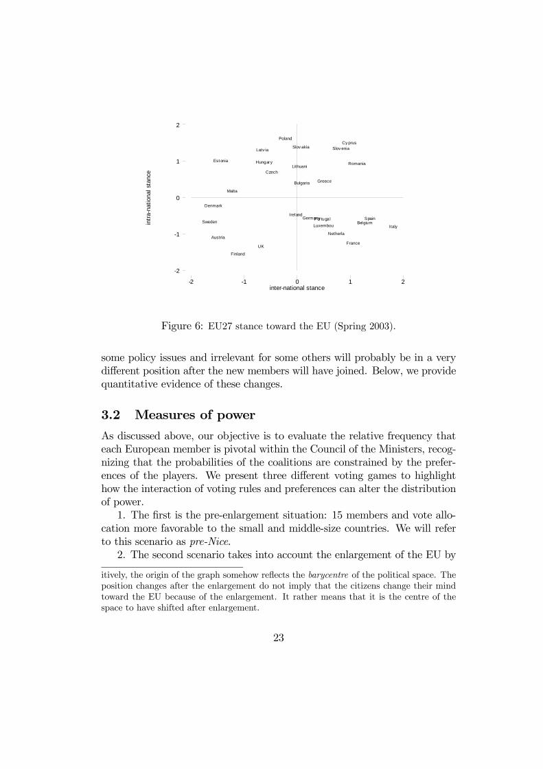
The EU 27 In regards to the 27 current and potential member coun-tries, the first two principal components also account for roughly 70% of thevariance in the data. We again found a similar pattern: that first factor isthe stance toward the EU on inter-national issues, while the second factor isthe stance toward the EU on domestic issues. The ideal points are presentedin figure 6.The newcomers from Eastern Europe tend to have generalized strong at-

titudes toward EU centralization in domestic policy domains (high intrana-tional stance). A certain degree of diversity is associated to the inter-nationalstance, probably due to mixed-feelings toward nationalism.A rapid comparison of figures 5 and 6 reveals that the “topology” of the

coalitions will change radically in the next few years, after enlargement. The“center” of the EU political space moves upwards, i.e., at least for intra-national issues, the average propensity to centralize the decision making atEuropean level raises consistently. Some old members that could be consid-ered relatively Euroenthusiasts become moderate, if not Euroskeptical afterenlargement.14 We expect that countries that were determinant (pivotal) for

14Observe that here we are talking about the relative attitudes of the countries towardthe EU. The coordinates of the graphs change as a result of the factoral analysis. Intu-

22

intra

-nat

iona

l sta

nce

inter-national stance-2 -1 0 1 2

-2

-1

0

1

2

Austria

Belgium

Bulgaria

Cy prus

Czech

Denmark

Est onia

Finland

France

Germany

Greece

Hungary

Ireland

Italy

Latv ia

Lithuani

Luxembou

Malta

Netherla

Poland

Portuga l

Romania

Slov akia Slov enia

SpainSweden

UK

Figure 6: EU27 stance toward the EU (Spring 2003).

some policy issues and irrelevant for some others will probably be in a verydifferent position after the new members will have joined. Below, we providequantitative evidence of these changes.

3.2 Measures of power

As discussed above, our objective is to evaluate the relative frequency thateach European member is pivotal within the Council of the Ministers, recog-nizing that the probabilities of the coalitions are constrained by the prefer-ences of the players. We present three different voting games to highlighthow the interaction of voting rules and preferences can alter the distributionof power.1. The first is the pre-enlargement situation: 15 members and vote allo-

cation more favorable to the small and middle-size countries. We will referto this scenario as pre-Nice.2. The second scenario takes into account the enlargement of the EU by

itively, the origin of the graph somehow reflects the barycentre of the political space. Theposition changes after the enlargement do not imply that the citizens change their mindtoward the EU because of the enlargement. It rather means that it is the centre of thespace to have shifted after enlargement.

23

the 12 potential members and the re-weighting agreed at Nice. This is whatwe call the post-Nice scenario. It has come into force starting from the firstenlargement round in May 2004.15

3. The third scenario is the Constitutional Treaty (CT). In June 2003,the Convention proposed abandoning the old weighted voting system andadopting a double majority based on both population and number of coun-tries.16

Pre-Nice — 15 Members Table 1 shows the results for the Pre-Nicescenario. It reports the standard Shapley-Shubik index (S-S), the normalizedBanzhaf index (NBI) and the spatial index in the Shapley-Owen perspective(S-O spatial). If we look at the S-O spatial values we see that the number ofvotes is no longer a good predictor of power. Shifting from standard S-S andNBI indices to the spatial value yields a concentration of power. This is dueto zero-probability assigned to a large number of ideologically non-consistentcoalitions.Since the qualified majority threshold is roughly 70%, we expect that

those countries who tend not to be “highly enthusiastic or completely reluc-tant” in participating coalitions on random political issues (i.e., say “yes”after the other countries have already cast almost the two-third of the votes)will have more chances to be pivotal. For such countries the spatial S-Opower index tends to be higher than the standard S-S or NBI indices. Con-versely, the power measure should decrease for countries who have extremepreferences (very strong or very little enthusiasm for Europe).Austria, Belgium, Spain, Germany and, surprisingly, Portugal gain sub-

stantial power from occupying favorable positions in the ideological space.

15Changes in votes allocation from pre-Nice situation to post-Nice can be seen by com-paring column two of tables 1 and 2 below. In the Treaty of Nice the qualified majoritythreshold was increased from 62 out of 87 to 255 out of 345.The Treaty of Nice prescribes also that bills are passed by the Council with two quotas: a

majority of states, and at least 62% of the total population of the Union. These additionalconditions produce negligible effects on winning coalitions. Then, we disregard in ouranalysis these and other complex aspects of the EU decision making, such as amendments,abstentions, etc.16The double majority sets two conditions for the passage of a bill: (a) more than 55%

of member states vote ”yes”; and (b) the population of the countries who have voted ”yes”represents at least 65% of the total population of the EU.For a limited number of issues, unanimity has been kept. Moreover, in the CT a sort of

safegard clause has been introduced. For simplicity we focus here on double majority.

24

The traditional view of a strong Central Europe led by the Franco-Germanaxis and supported by Belgium and the Netherlands is confirmed by the spa-tial approach. Little power rests upon the Northern countries. Denmark, isnever pivotal in any ideologically consistent coalition, whereas Finland andUK lose a lot of power from being “too skeptical” and “too close” each other.Also Greece and Italy lose power probably for the opposite reason of being“too enthusiastic.”In particular, for a given player, being close to another player can alter-

natively have two different consequences: (a) sharing the power with thatplayer that comes from occupying a certain portion of the space; (b) trans-ferring a substantial part of her own power to the other player, who oftensucceeds in being pivotal just before her or vice versa.

Country Votes S-S NBI S-O SpatialGermany 10 0.117 0.112 0.142Portugal 5 0.055 0.059 0.141Spain 8 0.095 0.092 0.118France 10 0.117 0.112 0.114Austria 4 0.045 0.048 0.092Belgium 5 0.055 0.059 0.083Netherlands 5 0.055 0.059 0.076Ireland 3 0.035 0.036 0.059UK 10 0.117 0.112 0.048Sweden 4 0.045 0.048 0.047Greece 5 0.055 0.059 0.045Italy 10 0.117 0.112 0.025Finland 3 0.035 0.036 0.009Luxembourg 2 0.021 0.023 0.003Denmark 3 0.035 0.036 0.000

Table 1: Power Values for Pre-Nice EU 15.

Post-Nice — 27 Members The enlargement is taking place under therules of Nice. Table 2 shows the big changes in the distribution of power afterthe full enlargement to 27 members. Again the standard indices are linearlycorrelated to the votes: 69% of the power measured by the Shapley-Shubikindex will be allocated to the current 15 members, whereas the six foundingstates will count for 31% of the power. However, once we shift to the spatial

25

Country Votes S-S NBI S-O SpatialCzech Rep 12 0.034 0.037 0.132France 29 0.087 0.078 0.101Germany 29 0.087 0.078 0.091Spain 27 0.080 0.074 0.089Greece 12 0.034 0.037 0.063Bulgaria 10 0.028 0.031 0.062Netherlands 13 0.037 0.040 0.054Lithuania 7 0.020 0.022 0.048Italy 29 0.087 0.078 0.048Poland 27 0.080 0.074 0.035Belgium 12 0.034 0.037 0.033Romania 14 0.040 0.043 0.030Portugal 12 0.034 0.037 0.024Slovakia 7 0.020 0.022 0.024Hungary 12 0.034 0.037 0.023Ireland 7 0.020 0.022 0.021Latvia 4 0.011 0.013 0.021Denmark 7 0.020 0.022 0.020Sweden 10 0.028 0.031 0.017UK 29 0.087 0.078 0.016Cyprus 4 0.011 0.013 0.014Austria 10 0.028 0.031 0.011Finland 7 0.020 0.022 0.010Slovenia 4 0.011 0.013 0.006Luxembourg 4 0.011 0.013 0.004Malta 3 0.008 0.009 0.003Estonia 4 0.011 0.013 0.000

Table 2: Power Values for Post-Nice EU 27.

approach, this broad idea of change becomes much more radical. Manycountries will lose a lot of their power as a consequence of their “unluckypositions” in the political space (see figure 6) and the unexpected result ispossibly the fact that these “losers” are more frequently current membersof the EU. UK’s spatial power decreases by more than 80% with respect toS-S index. Italy succeeds in being pivotal only in 4.8% of the ideologicallyconsistent coalitions. Austrian power falls by 61%. In general those countrieswith extreme preferences tend to lose in the political game: saying “yes” tooearly or too late is not a good idea when a 74% qualified majority has toform.The Franco-German axis is weaker: by requiring a higher qualified ma-

jority, Nice system subtracts the two big “moderate” countries a portion of

26

the usual power. Some of the traditional allies, such as Belgium and Luxem-bourg, are less powerful. In the future, the axis will probably need a highersupport from Spain, which emerges from Nice as a very strong player, dueto a very good position in the political arena.Differently from the old members, the majority of new entrants could

profit from favorable positions in the ideological space. The twelve newcom-ers collect a total 39.8% of the spatial power, despite the 30.8% quota ofstandard SS power and 31.3% of the votes. Too much enthusiasm penalizesPoland. Moreover, accessing countries are very close to each other in thepolitical area and Czech Republic is in a very good position at the centerof this Eastern-bloc. Thus we could predict an unexpected leading role forCzechs, whose 12 votes are enough to swing a large number of coalitions.

Constitutional Treaty The double majority system included in thenew Constitution is favorable to the four most populous countries, in termsof standard S-S and NBI power. Note from table 3 that S-S and NBI aresubstantially different: S-S is much more concentrated in the hands of thelargest six countries. This is due to a technical difference between S-S andNBI that becomes relevant in the case of double majority.17 A certain degreeof caution is then necessary when choosing one or the other index. Forexample, in the debate on the winners and losers under CT the commonperception has been that not only the four largest countries, but also thesmallest six would have gained from double majority with respect to Nice(Baldwin and Widgrén, 2004). Actually, this is true only if NBI evaluationsare used. S-S suggests that only the four largest members win, and all theothers lose.17As stated in section 2.1, Both S-S and NBI are symmetric indices. Differences between

them can arise from different values in the probabilities of the swung coalitions. In theBanzhaf’s perspective these probabilities are always the same and given by (3), whereasin Shapley and Shubik they are given by (2).CT prescribes that at least 15 members must be in the winning coalition. Intuitively,

the smallest countries tend to be pivotal thanks to this provision. Thus they are morelikely to swing coalitions that are “already” composed by 14 members. For such coalitions(3) is larger than (2). Thus, small countries’ power under CT tend to be emphasized byNBI evaluations.On the contrary, larger countries also swing coalitions that are composed by a larger

number of players and do not reach the population threshold. The probability assignedto such coalitions by S-S can be much larger than the one assigned by NBI. This explainswhy the S-S index of largest countries is much higher.

27

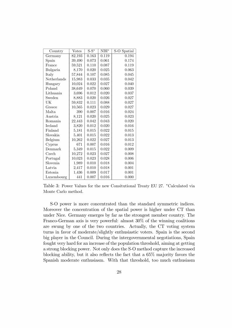
Country Votes S-S∗ NBI∗ S-O SpatialGermany 82,193 0.163 0.119 0.194Spain 39,490 0.073 0.061 0.174France 59,521 0.110 0.087 0.119Bulgaria 8,170 0.020 0.025 0.063Italy 57,844 0.107 0.085 0.045Netherlands 15,983 0.033 0.035 0.042Hungary 10,024 0.022 0.027 0.040Poland 38,649 0.070 0.060 0.039Lithuania 3,696 0.012 0.020 0.037Sweden 8,883 0.020 0.026 0.027UK 59,832 0.111 0.088 0.027Greece 10,565 0.023 0.029 0.027Malta 390 0.007 0.016 0.024Austria 8,121 0.020 0.025 0.023Romania 22,443 0.042 0.043 0.020Ireland 3,820 0.012 0.020 0.016Finland 5,181 0.015 0.022 0.015Slovakia 5,401 0.015 0.022 0.013Belgium 10,262 0.022 0.027 0.013Cyprus 671 0.007 0.016 0.012Denmark 5,349 0.015 0.022 0.009Czech 10,272 0.023 0.027 0.008Portugal 10,023 0.023 0.028 0.006Slovenia 1,989 0.010 0.018 0.004Latvia 2,417 0.010 0.018 0.001Estonia 1,436 0.009 0.017 0.001Luxembourg 441 0.007 0.016 0.000

Table 3: Power Values for the new Consitutional Treaty EU 27. ∗Calculated viaMonte Carlo method.

S-O power is more concentrated than the standard symmetric indices.Moreover the concentration of the spatial power is higher under CT thanunder Nice. Germany emerges by far as the strongest member country. TheFranco-German axis is very powerful: almost 30% of the winning coalitionsare swung by one of the two countries. Actually, the CT voting systemturns in favor of moderate/slightly enthusiastic voters. Spain is the secondbig player in the Council. During the intergovernmental negotiations, Spainfought very hard for an increase of the population threshold, aiming at gettinga strong blocking power. Not only does the S-Omethod capture the increasedblocking ability, but it also reflects the fact that a 65% majority favors theSpanish moderate enthusiasm. With that threshold, too much enthusiasm

28

can work against a country, such as Italy, that, despite its population, losesalmost two-thirds of its standard S-S power. The same rationale explainsthe loss by Poland or the Czech Republic. The new system is unfavorable toextremely skeptical countries: UK and Denmark lose most in terms of theirstandard S-S power. However, except for Denmark, the new Constitution isless penalizing to big Euroskeptics, compared to Nice.The Eastern bloc is less powerful than under Nice. The double major-

ity empathizes the role of population in power apportionment, while thenewcomers are small or middle-sized members. The ten Eastern countriesrepresent 22% of the EU population and collect 22.6% of spatial power. Forthem, in aggregate, the political locations turn to be unfavorable (-0.7% withrespect to the standard S-S power). CT prevents huge shifts of power towardEastern Europe that otherwise occur with Nice. The double majority distrib-utes the power more uniformly among the newcomers. The Czech Republicloses its leadership.Spatial values also explain why among the middle sized countries the

feelings toward CT have been mixed. Despite that for all of them NBIand S-S indices fall between 25-30%, some of them, such as Netherlands orAustria, gain in ideological values compared to Nice.Spain and Poland’s strong reluctance toward the Convention’s proposal

is inspired by losses both in terms of standard S-S and of spatial power:Nice favors Spanish and Polish pro-EU stance. The Convention had initiallyproposed a 60% population threshold that would have produced a relevantloss for the two countries. The agreement for the Constitution has beenreached thanks to a raising by 5 points in the two thresholds. If evaluated interms of standard symmetric power, this adjustment does not explain whySpain and Poland have accepted to sign the Constitution, since both their S-S and NBI values are lower under CT than Nice. The spatial power explainsmuch more: the raising of the thresholds allows Spain to be the second mostpowerful country in Europe and also improves the Polish position.The new Constitution restricts the areas (such as taxation, welfare, for-

eign policy, budget, justice) in which the unanimity of member countries isrequired. UK, Denmark or Finland, for example, are reluctant to abandonunanimity in those areas. The spatial power approach provides argumentsfor explaining those countries’ positions. In fact, if policy positions were dis-regarded, unanimity would imply equal power distribution. Thus we wouldnot be able to understand the strong opposition to unanimity by selectedcountries. Once we adopt the spatial approach, the power shifts in favor

29

of either Euroskeptics or Euroenthusiasts. In particular, unanimity allowscountries that are against centralization in sensitive policy domains (such astaxation for UK) to keep the highest amount of power.18

4 The agenda setter and power

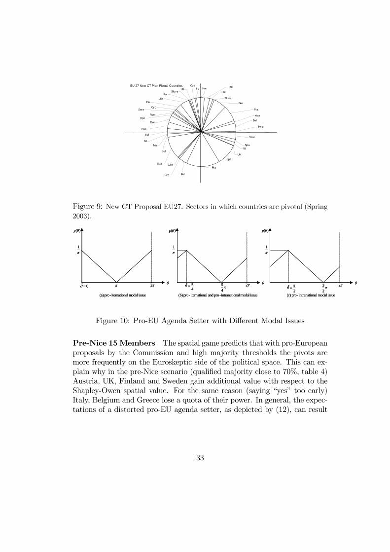
In section 2.5 we have argued that if there is an agenda setter, its most pre-ferred bills should be more likely than others, putting the pivots for morelikely bills in better positions. Within the EU legislative system the Commis-sion has the monopoly of the proposals for a large portion of issues, playingde facto the role of agenda setter. This can result in heavy distortion ofpower distribution within the Council.In the two-dimensional perspective developed in section 2.2.1: Ψ = H1,

the ordering generating function is fi(θ) = hθ, Pii, and the issue U is definedby θ ∈ [0, 2π). So far, in our application to the EU Council we have adoptedalso the Shapley-Owen’s hypothesis of equal relevance of policy issues. Inthis section we remove this hypothesis, and we introduce examples of non-uniform probability distribution over the set [0, 2π), and estimate the impacton power distribution.Since hereafter the issues can have different probabilities, we are inter-

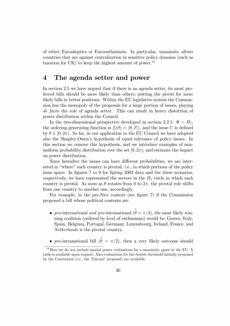
ested in “where” each country is pivotal: i.e., in which portions of the policyissue space. In figures 7 to 9 for Spring 2003 data and the three scenarios,respectively, we have represented the sectors in the H1 circle in which eachcountry is pivotal. As soon as θ rotates from 0 to 2π, the pivotal role shiftsfrom one country to another one, accordingly.For example, in the pre-Nice context (see figure 7) if the Commission

proposed a bill whose political contents are

• pro-international and pro-intranational (∧θ = π/4), the most likely win-

ning coalition (ordered by level of enthusiasm) would be: Greece, Italy,Spain, Belgium, Portugal, Germany, Luxembourg, Ireland, France, andNetherlands is the pivotal country.

• pro-intranational bill (∧θ = π/2), then a very likely outcome should

18Here we do not include spatial power evaluations for a unanimity game in the EU. Atable is available upon request. Also evaluations for the double threshold initially proposedby the Convention (i.e., the ’Giscard’ proposal) are available.

30

UK

Finland

Luxembourg

UK

Portugal

Sweden

Sweden

Greece

Ireland

Greece

SpainBelgium

Portugal

Netherlands

Spain

France

Italy

GermanyUK

France Austria

Netherlands

Ireland

ItalyAustria

Spain

EU 15 Pre-Nice Pivotal Countries

Figure 7: Pre-Nice EU15. Sectors in which countries are pivotal (Spring 2003).

be the coalition Greece, Portugal, Italy, Spain, Luxembourg, Ireland,Austria, Belgium, UK, and Germany, the pivotal country.

We know from section 2.5 that different expectations about the agendasetter’s type will result in different probability distributions over the set ofthe issues. In other words, the probability distribution over the set [0, 2π)of all the possible bills can be anticipated by looking at the Commission’sdecision making.We assume a simple linear probability density function

p(θ) =

⎧⎪⎪⎪⎨⎪⎪⎪⎩hθ + (π − bθ)i /π2 if 0 ≤ θ < bθ

(1/π)−³θ − bθ´ /π2 if bθ ≤ θ < π + bθh

θ − (π + bθ)i /π2 if π + bθ ≤ θ < 2π

⎫⎪⎪⎪⎬⎪⎪⎪⎭ (12)

∧θ is what the players expect as the most preferred issue by the Commis-

sion. Function (12) says that the probability density of a proposal θ willincrease linearly as θ approaches bθ. Moreover the probability density falls tozero with regards to the opposing issue bθ + π.We further assume that the Commission prefers to promote integration

with respect to the status quo. Thus the countries expect bθ to lie in £0, π2

¤.

We further suppose that the following three distributions reflect alternativepriors of the states about the Commission’s decision making.

31

Cze Hun Ger Neth

Est

Pol UK

Fin CzeSlova

AusLith

Swe

Slove

Den Rom

Cze

Gre Hun

Ita

Gre

Bel Spa Pol

Slova GreFra Bel

Spa

UK

Ger Fra

Den Neth

Swe Lux

Ita

Ita

EU 27 Nice Proposal Pivotal

Figure 8: Post-Nice EU27. Sectors in which countries are pivotal (Spring 2003).

• For a purely pro-international modal issue:∧θ = 0; we show the graph

of this version of equation (12) in figure 10(a) below.

• Alternatively, if the Commission preferred issues that are pro-internationaland pro-intranational, we would expect a density function with mode

in∧θ = π/4, whose graph is represented in figure 10(b).

• If the most preferred issue is purely pro-intranational, thus∧θ = π/2

and the probability distribution will be as in 10(c).

Of course, these are just examples of our ad hoc probability distribu-tion. Nonetheless they can capture alternative behavior and preferences ofthe agenda setter and get a reliable idea on how the power shifts from someplayers to others as a result of the action of the agenda setter. In moresophisticated cases we could have density functions with different or multi-ple modal values, or non-linear relations between issues and probability. Ingeneral, we could wonder how the voter can infer the distribution from thelimited information about the agenda setter’s type; but this is beyond thetasks of this paper.19

19Note also that function (12) can reflect our assumptions only if∧θ ∈ [0, π]. This is not

a problem since we have additionally supposed that∧θ ∈ [0, π/2].

32

Fin

CypSw e

RomDen

Gre

Aus

Bul

Bul

Ita Mal

Spa

Gre

Cze

Pol

Fra

Spa

Ita

UK

Spa

Sw e

LithPor

Slova UK

CzeIre Hun

Bul

Pol

Slova

Ger

Fra

Aus

Bel

Sw e

EU 27 New CT Plan Pivotal Countries

Figure 9: New CT Proposal EU27. Sectors in which countries are pivotal (Spring2003).

π45

)(θp

4ˆ πθ =

π1

θπ2

issue modal nalintranatio-pro and aliternation-pro (b)

π

)(θp

0ˆ =θ

π1

θπ2

issue modal aliternation-pro (a)

π23

)(θp

2ˆ πθ =

π1

θπ2

issue modal nalintranatio-pro (c)

π45

)(θp

4ˆ πθ =

π1

θπ2

issue modal nalintranatio-pro and aliternation-pro (b)

π

)(θp

0ˆ =θ

π1

θπ2

issue modal aliternation-pro (a)

π23

)(θp

2ˆ πθ =

π1

θπ2

issue modal nalintranatio-pro (c)

Figure 10: Pro-EU Agenda Setter with Different Modal Issues

Pre-Nice 15Members The spatial game predicts that with pro-Europeanproposals by the Commission and high majority thresholds the pivots aremore frequently on the Euroskeptic side of the political space. This can ex-plain why in the pre-Nice scenario (qualified majority close to 70%, table 4)Austria, UK, Finland and Sweden gain additional value with respect to theShapley-Owen spatial value. For the same reason (saying “yes” too early)Italy, Belgium and Greece lose a quota of their power. In general, the expec-tations of a distorted pro-EU agenda setter, as depicted by (12), can result

33

Country θ̂ = 0 θ̂=π/4 θ̂=π/2

Austria 0.136 0.129 0.091Belgium 0.048 0.035 0.074Denmark 0.000 0.000 0.000Finland 0.014 0.010 0.005France 0.052 0.106 0.162Germany 0.089 0.145 0.195Greece 0.055 0.040 0.035Ireland 0.085 0.069 0.043Italy 0.019 0.016 0.015Luxembourg 0.005 0.003 0.002Netherlands 0.075 0.104 0.106Portugal 0.192 0.154 0.118Spain 0.096 0.064 0.043Sweden 0.074 0.068 0.058UK 0.061 0.058 0.055

Table 4: Probabilistic Spatial Values with Different Types of Agenda Setter (pre-Nice EU 15)

in 9.8% redistribution of the total S-O power.20

Post-Nice 27 Members The EU 27 scenario resulting from Nice votingrules is more complex. We have already remarked that the accession ofmany Euroenthusiasts will shift the “center” of the political space towardEuroenthusiasm, making the current members relatively more Euroskeptic.Thus, the countries who gain from pro-EU proposals are more frequentlycurrent members (Germany, Ireland, UK, Austria, Finland, Italy.). Thismitigates the risk of large concentration of S-O power on the so-called Easternbloc.Due to the large number of members and to the relatively high majority

threshold agreed at Nice (around 74%) the pivotal role can rapidly pass fromone country to another one as the proposal changes. This makes more than34% of the allocation of spatial power to depend upon the agenda setter’spreferences, as given by (12). In other words, raising the majority threshold

20Intuitively, the amount of power redistribution is negatively related to the variance ofthe probability distribution of the issues: when the agenda setters’ proposals are easy topredict, the probability of playing a pivotal role is concentrated.

34

Country θ̂ = 0 θ̂=π/4 θ̂=π/2Austria 0.007 0.015 0.023Belgium 0.020 0.012 0.015Bulgaria 0.053 0.065 0.083Cyprus 0.007 0.013 0.019Czech 0.029 0.034 0.046Denmark 0.005 0.019 0.034Estonia 0.016 0.028 0.041Finland 0.017 0.018 0.019France 0.097 0.069 0.047Germany 0.277 0.279 0.214Greece 0.012 0.012 0.017Hungary 0.006 0.008 0.008Ireland 0.023 0.046 0.070Italy 0.086 0.068 0.062Latvia 0.016 0.021 0.029Lithuania 0.029 0.035 0.048Luxembourg 0.000 0.000 0.000Malta 0.000 0.002 0.003Netherlands 0.041 0.035 0.021Poland 0.001 0.002 0.002Portugal 0.069 0.063 0.044Romania 0.051 0.037 0.023Slovakia 0.022 0.014 0.012Slovenia 0.007 0.012 0.016Spain 0.037 0.035 0.055Sweden 0.002 0.005 0.008UK 0.069 0.056 0.043

Table 5: Probabilistic Spatial Values with Different Types of Agenda Setter (Post-Nice EU 27)

increases the influence of the Commission upon the power equilibria into theCouncil. The results are presented in table 5.

Constitutional Treaty The CT reduces the qualified majority to 65%,provided at least 15 members have voted “yes”. This lowering has at least twoeffects: it makes the pivotal role of moderate countries more likely; it reducesthe sensitivity of power distribution to the agenda setter’s proposals. Whenthe Commission turns from indifference to pro-EU attitude ’only’ 16.9% oftotal S-O power is reallocated.Still Germany, Spain and France are very powerful, however Bulgaria and

35

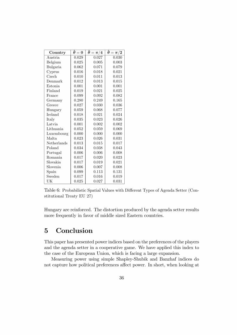
Country θ̂ = 0 θ̂ = π/4 θ̂ = π/2Austria 0.029 0.027 0.030Belgium 0.025 0.005 0.003Bulgaria 0.062 0.071 0.079Cyprus 0.016 0.018 0.021Czech 0.010 0.011 0.013Denmark 0.012 0.013 0.015Estonia 0.001 0.001 0.001Finland 0.019 0.021 0.025France 0.099 0.092 0.082Germany 0.280 0.249 0.165Greece 0.027 0.030 0.036Hungary 0.059 0.068 0.077Ireland 0.018 0.021 0.024Italy 0.035 0.023 0.026Latvia 0.001 0.002 0.002Lithuania 0.052 0.059 0.069Luxembourg 0.000 0.000 0.000Malta 0.023 0.026 0.031Netherlands 0.013 0.015 0.017Poland 0.034 0.038 0.043Portugal 0.006 0.006 0.008Romania 0.017 0.020 0.023Slovakia 0.017 0.019 0.021Slovenia 0.006 0.007 0.008Spain 0.099 0.113 0.131Sweden 0.017 0.016 0.019UK 0.025 0.027 0.031

Table 6: Probabilistic Spatial Values with Different Types of Agenda Setter (Con-stitutional Treaty EU 27)

Hungary are reinforced. The distortion produced by the agenda setter resultsmore frequently in favor of middle sized Eastern countries.

5 Conclusion

This paper has presented power indices based on the preferences of the playersand the agenda setter in a cooperative game. We have applied this index tothe case of the European Union, which is facing a large expansion.Measuring power using simple Shapley-Shubik and Banzhaf indices do

not capture how political preferences affect power. In short, when looking at

36

possible coalition formation, countries who are relatively ’pro’ a particularissue will be more likely to vote ’yes’ before those countries who are ’con.’Majorities formed by pro-countries are more likely than majorities formedby con-countries. Being able to swing a large number of coalitions puts thevoter in a powerful position only if those coalitions are also likely to occur.More likely coalitions are those ones that include similarly minded voters.Thus the power of countries will be determined not only by the number ofvotes they have and the number of votes needed for a majority, but also bythe attitudes that the countries hold. In cases where unanimity is needed, forexample, the most ’con’ countries hold the most sway. In games, where a two-thirds majority is needed countries who are moderately ’con’ then becomemore powerful since the likelihood of them joining the coalition ’too early’ issmall.The attitudes that create political coalitions depend also on the content

of the issue to vote on. If the issue is proposed by an agenda setter, theagenda setter’s preferences can distort the likelihood of the coalitions andultimately the distribution of power.Using principal components analysis we are able to extract countries’

attitudes toward the EU. These attitudes are then used to create what we callthe spatial Shapley-Owen index. Our results show, for example, that countrieswith the greatest number of votes (and hence highest simple Shapley-Shubikindices) do not necessarily have the greatest power after considering theirpreferences.The spatial approach captures the current leadership of the Franco-German

axis and the political weakness of Northern Euroskeptics and MediterraneanEuroenthusiasts. After enlargement the “positions” in the political space willbecome even more relevant as a source of power, and, if the Nice rules are notchanged, the Western members will frequently occupy unfavorable positions.The closeness of the new members will result in a strong Eastern politicalbloc.The double majority included in the CT restores concentration of power

in favor of big and politically moderate members; the Eastern bloc is lesspowerful. Lowering the majority threshold causes those countries with ex-treme preferences to suffer more.In our spatial political games we have modeled the agenda setter’s pref-

erences through an ad hoc distribution which assigns higher probability topro-European issues. We find that with higher majority thresholds the EUCommission’s preferences can have a larger impact on the power distribu-

37

tion, i.e., a greater share of power can change hands. Under Nice the riskof distortions of the European political game caused by the Commission’sproposals is high. This risk grows when the number of members increasesand when there is little uncertainty about the Commission’s preferences.Within the debate on the institutional reforms of the EU, our findings

show the need for a serious reflection about the strong concentration of thelegislative prerogatives within the Council and about the recognition of agreater political role to the Commission.In summary, the measurement of power based on preferences leads to in-

teresting and sometimes unexpected results, which can be used as an a priorimeasure of the prospect of participating in a political game. Nonetheless, acertain degree of caution is necessary. Some paradoxical situations of thespatial voting theory, such as the median voter paradox, can emerge in themeasurement of the spatial values. Moreover, the spatial power indices seemto be quite responsive to slight differences in preference measurement. Alsoexogeneity of preferences can be challenged if, for example, the voters canchose their political position aiming at maximizing their power. Finally, sincewe use the preferences of the citizens to evaluate the political location of therepresentatives, a principal-agent problem could arise between citizens andtheir elected representatives. We leave these aspects for future work.

38

6 Appendix A: Eurobarometer survey ques-tions

The Eurobarometer survey covers the population of the EU member states.The basic sample design consists of a number of sampling points that areproportional to the population size and density. In each country almost 1,000face-to-face interviews are carried out. We use three Eurobarometer surveys(Fall 2001, Fall 2002 and Spring 2003). The part of the interview which isrelevant for our analysis is the one which concerns the opinions of the peoplewhether to centralize some policy domains, which is based on the followingquestion: ”For each of the following area, do you think that decisions shouldbe made by the (NATIONALITY) government, or made jointly within theEuropean Union?” (EC 2003)21

7 Appendix B: Data analysis

7.1 Principal components

Factor models have been used in economic analysis and forecasting to reducethe dimensionality of large data sets. We apply the standard techniques offactor analysis/principal components using Stata 8.0. In our analysis we have25 variables, xi, i = 1, ..., p(= 25), with a considerable degree of (positive)correlation among these variables. This leads to the use of factor analysis tocapture underlying, latent variables that can account for this high degree ofcorrelation among these variables. The aim of factor analysis is to account forthe covariances of the observed variables in terms of a much small numberof hypothetical variables, fr, r = 1., , , k; k << 25, such that the partialcorrelation coefficients between the original variables after eliminating theeffect of f 0rs are close zero. Each variable, xi is modeled as a linear functionof k common ’factors’ or latent variables:

xi =kX

r=1

λirfr + µi, i = 1, ..., p, (13)

where fr ∈ f is the rth common factor, k is the number of factors being spec-ified, µi is a residual source of variation affecting only xi, and the coefficients21We exluded the Terrorism variable since we did not have a response for this variable

for all 27 countries.

39

Issues1 Defense2 Protection of the environment3 Currency4 Humanitarian aid5 Health and social welfare6 Basic rules for broadcasting and press7 Fight against poverty/social exclusion8 The Fight Against Unemployment9 Agriculture and fishing policy10 The support of regions which are experiencing economic difficulties11 Education12 Scientific and technological research13 Information about the EU, its policies and institutions and bodies14 Foreign policy towards countries outside the EU15 Cultural policy16 Immigration policy17 Rules for political asylum18 The fight against organized crime19 Police20 Justice21 Accepting refugees22 Juvenile crime prevention23 Urban crime prevention24 The fight against drugs25 The fight against the trade in, and exploitation of, human beings26 The fight against international terrorism

Table 7: Eurobarometer survey questions.

λir ∈ Λare called the factor loadings of xi on fr.The method of principal components minimizes

V (k) = minΛ,f

ÃpX

i=1

"xi −

kXr=1

λirfr

#!2, i = 1, ..., p

The estimated factors, f̂r, are the eigenvectors corresponding to the k

largest eigenvalues of the matrix xx0, and Λ̂ =³f̂ f̂0´xf̂

0are the corresponding

factor loadings. If we denote δr, r = 1, ..., k the eigenvalue for the rth factor,then each factor explains δr/p proportion of the total variance in the dataset (since

Ppr=1 δr = p). We have chosen k = 2 in order to measure power

40

values for each country in two dimensions; however, the two factors explainover 70% of the variance in the data sets.Furthermore in cases where k > 1, there are an infinite number of choices

for Λ. Thus to elicit clearer patterns in the data, we use the varimax rotationprocedure, whereby we ’rotate’ the factors in such a way that the new loadingstend to be either relatively large or small in absolute size compared with theoriginal ones. Since each factor is a vector of correlation coefficients, themost interpretable factor is one based upon correlation coefficients which areeither close to one in absolute value or close to zero in absolute value (Lawleyand Maxwell, 1971).We can then inspect the rotated factor loadings to see which of the original

variables are most highly correlated with each of the factors. Inspectionof the loadings shows that, in general, that the first factor is most highlycorrelated with international issues, while the second factor is associated withdomestic/internal issues. Next the factors are then ’scored’, which assignsweights for the contribution of each variable to the factor. The mean of eachthe scored factor is zero and the standard deviation is 1. Each scored factorfor each country is plotted in figures 5 and 6 above (Lawley and Maxwell,1971).

7.2 PCAs Spring 2003

Given our data set, principal component analysis gives the following tables,where table 8 reports the results for EU 15 for Spring 2003, and table 9 reportsresults for EU 27, Spring 2003. Each value for each variable is a correlationcoefficient that measures by how much the variable is correlated with therespective factor. Looking at which variables are more highly correlatedwith each factor allows us to give an interpretation to each factor (i.e., theintra-national and inter-national factors).

8 Appendix C: Shapley-Owen spatial valuecalculation

This section gives more description of how we calculate the Shapley-Owenspatial value. For a given year, first we calculate the scored factors for EU15 and EU 27, as described above. The scored factors are plotted in figure

41

Variable Factor 1 Factor 2defence 0.67 0.41environment 0.82 0.36currency 0.56 0.38humanitarian aid 0.72 0.44health and social welfare 0.28 0.89media 0.08 0.64poverty and social exclusion 0.47 0.61unemployment 0.40 0.74agriculture 0.83 0.14regional aid 0.13 0.32education 0.38 0.80research 0.61 0.65information 0.71 0.25foreign policy 0.73 0.47cultural policy 0.28 0.69immigration 0.77 0.59political asylum 0.74 0.60organized crime 0.76 -0.02police 0.41 0.85justice 0.47 0.81accepting refugees 0.74 0.54juvenile crime 0.10 0.91urbancrime -0.15 0.84drugs 0.72 0.26exploitation of human beings 0.94 -0.03

Table 8: Rotated factors for EU 15 (Spring 2003).

5 and 6. For each country, we then calculate its relative ”pro-con” value for10, 000 points from zero to 2π using the formula:

yi = f1i cos θ + f2i sin θ, θ ∈ [0, 2π] , i = 1, .., n

where yi is a country i0s relative sentiment (ranking) on issue θ, and n isthe number of countries (either 15 or 27) and f1i and f2i are the two factorsfor each country. We use 10, 000 values of θ in the [0, 2π] range in order toget many rankings, which will insure us that we catch all of the ’switchingpoints,’ i.e., the points along [0, 2π] where the relative rankings of countries’preferences change.For each θ, we rank yi, i = 1, ..n, from highest to lowest (i.e., most pro

to most con), and record at what values of θ the rankings change. Thenwe calculate the pivotal voters—given the particular rules of the game—and

42

Variable Factor 1 Factor 2defence 0.45 0.65environment 0.54 0.61currency 0.66 0.23humanitarian aid 0.66 0.55health and social welfare 0.34 0.88media 0.62 0.34poverty and social exclusion 0.33 0.87unemployment 0.22 0.94agriculture 0.49 0.65regional aid 0.07 0.80education 0.22 0.90research 0.48 0.76information 0.46 0.70foreign policy 0.86 0.23cultural policy 0.82 0.09immigration 0.83 0.43political asylum 0.88 0.32organized crime 0.24 0.79police 0.42 0.83justice 0.47 0.79accepting refugees 0.90 0.28juvenile crime 0.33 0.83urbancrime 0.23 0.73drugs 0.16 0.91exploitation of human beings 0.30 0.74

Table 9: Rotated factors EU 27 (Spring 2003).

record the interval length for which each country is pivotal. To calculatethe Shapley-Owen spatial value we add the length of the pivotal intervals foreach country. Lastly we normalize the results so the sum of power values isequal 1.To calculate the power-values using a non-uniform distribution, we first

take the length of the intervals along [0, 2π] for which each country is pivotal.For each interval we take the integral using equation (12). We then sum theintegrals for each country and normalize them to get the power values.We repeat each of the steps for the three years and take average of the

Shapley-Owen spatial values. The calculations were done in Mathematica3.0. The code is available upon request.

43

References

[1] Alesina, A. F. I. Angeloni and L. Schuknecht (2002), “What Does theEuropean Union Do?”, CEPR Discussion Paper no. 3115, London.

[2] Alesina, A. and R. Perotti (2004), “The European Union: A PoliticallyIncorrect View”, Journal of Economic Perspectives, Vol. 18, No. 4, pp.27-48.

[3] Baldwin, R. E. Berglof, F. Giavazzi and M. Widgrén (2001), Nice Try:Should the Treaty of Nice Be Ratified? CEPR , London.

[4] Baldwin, R. E. and M. Widgrén, (2004), Winners and losers undervarious dual majority rules for the EU’s Council of Ministers, (mimeo).

[5] Banzhaf, John F. III (1965), “Weighted Voting doesn’t Work: A Math-ematical Analysis”, Rutgers Law Review, 19, pp. 317-343.

[6] Berglof, E. B. Eichengreen, G. Roland, G. Tabellini, C. Wyplosz (2003),Built to Last: a Political Architecture for Europe, CEPR series, Moni-toring European Integration, No. 12, London.

[7] European Commission (2003), http://europa.eu.int/comm/public_opinion,March, B66-B68.

[8] Felsenthal, D.S. and Machover, M. (1998), The Measurement of VotingPower, Edward Elgar Publ., Oxford.

[9] Felsenthal, D. S. and M. Machover (2001), “The Treaty of Nice andQualified Majority Voting”, Public Choice and Welfare, 18, pp. 431-464.

[10] Holler M. J. and G. Owen, editors (2001), Power Indices and CoalitionFormation, Kluwer Academic Publisher, Boston.

[11] Lawley, D. N. andMaxwell, A. E. (1971), Factor Analysis as a StatisticalMethod. American Elsevier Publishing: New York.

[12] Monderer, D. and Samet, D. (2002), “Variations on the Shapley Value”in Handbook of Game Theory, vol. 3, R. J. Aumann and S. Hart, editors,Elsevier Science B. V., pp. 2055-2076.

44

[13] Napel, S. and M. Widgrén (2003), EU Conciliation Committee: Council56 vs. Parliament 6, CEPR, London.

[14] Noury, A. and G. Roland (2002), “More Power to the European Parlia-ment?”, Economic Policy, 35, pp. 281-319.

[15] Owen, G. (1972), “Political Games”, Naval Research Logistics Quarterly,18, pp. 345-354.

[16] Owen, G. (1975), “Evaluation of a Presidential Election Game”, Amer-ican Political Science Review, 69, pp. 947-953.

[17] Owen, G. and L. S. Shapley (1989), “Optimal Location of Candidatesin Ideological Space”, International Journal of Game Theory, 18, pp.339-356.

[18] Persson, T. and G. Tabellini (2003), The Economic Effects of Constitu-tions, The MIT Press, Cambridge, MA.

[19] Rabinowitz, G. and S. E. Macdonald (1986), “The Power of the Statesin U. S. Presidential Elections”, American Political Science Review, 80,pp. 65-87.

[20] Rapoport, A. and E. Golan (1985), “Assessment of Political Power inthe Israeli Knesset”, American Political Science Review, 79, pp. 673-692.

[21] Romer, T. and H. Rosenthal, (1978), “Political Resource Allocation,Controlled Agendas, and the Status Quo”, Public Choice, 33, pp. 27-44.

[22] Rosenthal, H. (1990), “The Setter Model”, in Advances in the SpatialTheory of Voting, J. M. Enelow and M. J. Hinich, editors, CambridgeUniversity Press, Cambridge, pp. 199-232.

[23] Shapley, L. S. (1953), “A Value for n-Person Games” in Contributionsto the Theory of Games, vol. II, H. W. Khun and A. W. Tucker, ed-itors, Annals of Mathematics Studies, 28, Princeton University Press,Princeton, pp. 307-317.

[24] Shapley, L. S. (1977), “A Comparison of Power Indices and a Nonsym-metric Generalization”, Paper P-5872, The Rand Corporation, SantaMonica.

45

[25] Shapley, L. S. and M. Shubik (1954), “A Method for Evaluating the Dis-tribution of Power in a Committee System”, American Political ScienceReview, 48, pp. 787-792.

[26] Straffin, P. D. (1994), “Power and Stability in Politics” in Handbookof Game Theory, vol. 2, R. J. Aumann and S. Hart, editors, ElsevierScience B. V., pp. 1127-1151.

[27] Weber, R. J. (1988), “Probabilistic Values for Games”, in The ShapleyValue: essays in honor of Lloyd S. Shapley, A. E. Roth, editor, Cam-bridge University Press, Cambridge, pp. 101-119.

[28] Widgrén, M. (1994), “Voting Power in the EC and the Consequencesof Two Different Enlargements”, European Economic Review, 38, pp.1153-1170.

46