Window-Related Energy Consumption in the US Residential and Commercial Building Stock Joshua Apte and Dariush Arasteh, Lawrence Berkeley National Laboratory LBNL-60146

Abstract We present a simple spreadsheet-based tool for estimating window-related energy consumption in the United States. Using available data on the properties of the installed US window stock, we estimate that windows are responsible for 2.15 quadrillion Btu (Quads) of heating energy consumption and 1.48 Quads of cooling energy consumption annually. We develop estimates of average U-factor and SHGC for current window sales. We estimate that a complete replacement of the installed window stock with these products would result in energy savings of approximately 1.2 quads. We demonstrate that future window technologies offer energy savings potentials of up to 3.9 Quads. Introduction According to the US Department of Energy, in 2003 space conditioning in residential and commercial buildings was responsible for 9.19 quadrillion Btu (Quads) of site energy consumption, and 12.03 Quads of primary (source) consumption (US DOE Office of Energy Efficiency and Renewable Energy 2005). Although windows are generally understood to be an important driver of space conditioning energy consumption, few studies have directly investigated the energy impacts of windows at the national level. In this study, we introduce a simple spreadsheet-based tool for estimating the national energy impacts of windows in residential and commercial buildings. After presenting estimates of current window-related energy consumption in the US building stock, we discuss the energy savings potential of various technology scenarios. Methods and Results This section is divided into two sub-sections. In the first section, we describe the techniques and assumptions involved in estimating the window-related energy consumption of the US building stock. In the second section, we describe the process we used to estimate the energy-savings potential of various window technologies. Window-Related Energy Consumption of Building Stock General Approach In order to estimate the energy consumption attributable to the US window stock, we used a combination of top-down and bottom-up approaches. First, we compiled a set of estimates of total space conditioning energy consumption in the US building stock, broken down by sector (residential, commercial) and conditioning mode (heating, cooling). Second, for each of these four aggregated end use categories, we combined building energy simulations with market and survey data to estimate the fraction of total energy consumption attributable to windows. We then estimated the window-related space conditioning energy consumption for each end use category by multiplying total space conditioning energy consumption by the window-related fraction of that

1

consumption. Finally, we determined a total national estimate by summing across the four end use categories. This approach is formalized below in Equation 1. Equation 1

∑ ⎟⎠⎞⎜

⎝⎛ ×=

E.S

StockES,AWFStock

ES,THEStockTWE

where: TWE (“Total Window Energy”) represents the total-window related primary energy consumption of the US building stock. THE (“Total HVAC Energy”) represents the total primary HVAC energy consumption for a given end use in a given sector in the US building stock. S represents a given sector of the US building stock (Residential or Commercial). E represents a given end use for space conditioning energy (heating or cooling). AWF (“Aggregate Window Fraction”) represents the window-related fraction of space conditioning energy consumption (heating, cooling) for a given stock segment (residential, commercial).

National Energy Consumption Estimates We used estimates of building space conditioning energy consumption published in the 2005 DOE Buildings Energy Databook as the starting point for our analysis, as presented in Table 1. In the following sections, we estimate the fraction of this energy consumption attributable to the installed window stock in residential and commercial buildings. We then estimate how this fraction would change under a variety of window technology scenarios. Table 1 - Space Conditioning Energy Consumption in US Buildings

Annual HVAC Energy Consumption Quadrillion Primary BTU (quads)1End Use

Residential Buildings Commercial Buildings Heating 6.90 2.45 Cooling 2.41 1.90

Total 9.31 4.35 Window Fraction of Total Energy Consumption Background Although the effects of windows on energy consumption are well understood at the building level, few studies have attempted a detailed characterization of the national energy impacts of windows. This limitation can be explained by several factors. First, the energy impacts of windows, even at the building level, are difficult to quantify without extensive monitoring and instrumentation. Computer energy simulations therefore offer a far more practical approach; however, the US building stock is highly heterogeneous, meaning dozens if not hundreds of models are required. Moreover, the composition and

1 The term “Quad” is shorthand for 1 quadrillion (1015) Btu = 1.056 EJ. “Primary” energy consumption includes a site-to-source conversion factor of 3.22 for electricity to account for losses in transmission, distribution, and generation. All energy consumption is reported in primary terms unless otherwise noted.

2

properties of the US building stock are poorly characterized with respect to shell integrity and energy efficiency. Detailed descriptions of the installed window stock are nonexistent. The most detailed datasets tend to be limited to a particular geographical region, while those with a national scope often leave key questions unanswered. In order to estimate the fraction of building space conditioning energy consumption attributable to windows, we conducted a reanalysis of two simulation studies of building HVAC loads originally conducted by Joe Huang and others at Lawrence Berkeley National Laboratory (Huang and Franconi 1999; Huang et al. 1999). These studies relied on an extensive set of DOE-2 models (“prototypical buildings” or “prototypes”) designed to capture the diversity of the US residential and commercial building stock. Using parametric simulations, the authors determined the relative contribution of internal heat gains and building envelope components to total space conditioning loads for each prototypical building. By weighting these building-level estimates with stock size data derived from the EIA Residential- and Commercial Building Energy Consumption Surveys (RECS, CBECS), the authors then developed aggregate estimates of total “component loads” for the US building stock. General Procedure We used prototype-level simulation results2 published in Huang et al. (1999) and Huang and Franconi (1999) as a starting point for our analysis. These results estimate space conditioning loads attributable to each of a set of internal and envelope components for 80 prototypical residential buildings and 120 prototypical commercial buildings. We term these loads “component loads”, and a list of the building component loads simulated in this study can be found in Table 10. We entered these loads into separate spreadsheets for residential and commercial buildings, with separate tables for heating loads and cooling loads. In order to estimate the percentage of space conditioning energy consumption attributable to windows for each of these end use categories, we used a six – step process. This process is briefly outlined below (see Figure 1 for a graphical representation) and explained in greater detail in the Residential Buildings and Commercial Buildings subsections.

- First, we categorized the component loads derived by Huang et al. into those that were at least partly attributable to windows (infiltration, window conduction, and window solar gain), and those that were not. For simplicity, we collapsed the loads unrelated to windows into a “non-window” category.

- Second, we used the most recent RECS and CBECS surveys to generate estimates of the size of the US building stock corresponding to each of Huang et al.’s prototypical buildings. We used these size estimates to determine the window-related and total loads at the national level that correspond with each of the 320 prototypical buildings simulated by Huang et al.

- Third, we used prototypical building-specific “efficiency factors” derived by Huang et al. to estimate the primary (source) energy consumption necessary to meet space conditioning loads.

2 A list of all prototype buildings can be found in Table 9.

3

- Fourth, we used information from proprietary market research to generate up-to-date estimates of window energy efficiency that reflect the properties of today’s window stock. As the assumed window properties of the prototype buildings used in the Huang studies differed from these values, we applied a set of correction factors to the window-related component loads.

- Fifth, we aggregated window and total loads across all building types to develop a set of aggregate space conditioning load estimates for the entire commercial and residential building stocks.

- Finally, we used these aggregated estimates to estimate the window-related fraction of building space conditioning energy consumption in residential and commercial buildings. This value was calculated by dividing the aggregate window-related load by the aggregate total load.

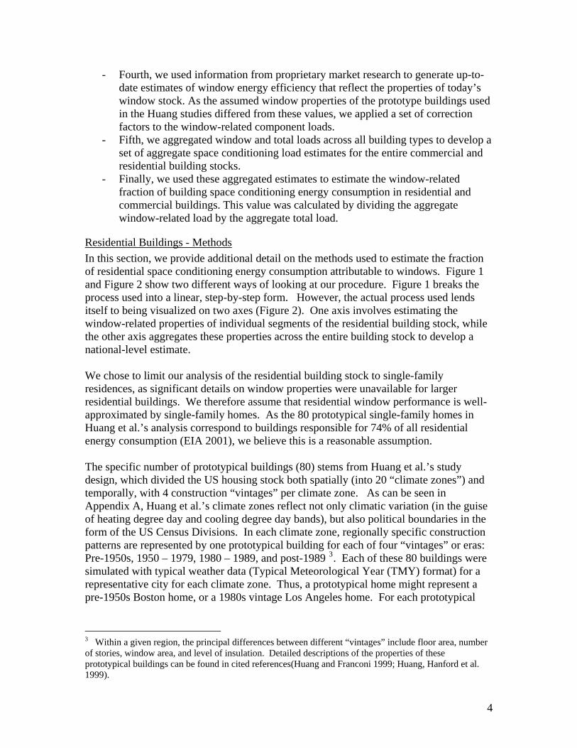
Residential Buildings - Methods In this section, we provide additional detail on the methods used to estimate the fraction of residential space conditioning energy consumption attributable to windows. Figure 1 and Figure 2 show two different ways of looking at our procedure. Figure 1 breaks the process used into a linear, step-by-step form. However, the actual process used lends itself to being visualized on two axes (Figure 2). One axis involves estimating the window-related properties of individual segments of the residential building stock, while the other axis aggregates these properties across the entire building stock to develop a national-level estimate. We chose to limit our analysis of the residential building stock to single-family residences, as significant details on window properties were unavailable for larger residential buildings. We therefore assume that residential window performance is well-approximated by single-family homes. As the 80 prototypical single-family homes in Huang et al.’s analysis correspond to buildings responsible for 74% of all residential energy consumption (EIA 2001), we believe this is a reasonable assumption. The specific number of prototypical buildings (80) stems from Huang et al.’s study design, which divided the US housing stock both spatially (into 20 “climate zones”) and temporally, with 4 construction “vintages” per climate zone. As can be seen in Appendix A, Huang et al.’s climate zones reflect not only climatic variation (in the guise of heating degree day and cooling degree day bands), but also political boundaries in the form of the US Census Divisions. In each climate zone, regionally specific construction patterns are represented by one prototypical building for each of four “vintages” or eras: Pre-1950s, 1950 – 1979, 1980 – 1989, and post-1989 3. Each of these 80 buildings were simulated with typical weather data (Typical Meteorological Year (TMY) format) for a representative city for each climate zone. Thus, a prototypical home might represent a pre-1950s Boston home, or a 1980s vintage Los Angeles home. For each prototypical

3 Within a given region, the principal differences between different “vintages” include floor area, number of stories, window area, and level of insulation. Detailed descriptions of the properties of these prototypical buildings can be found in cited references(Huang and Franconi 1999; Huang, Hanford et al. 1999).

4

building, the contribution of the following components to total HVAC load was estimated:

Roof Wall Window Solar Gain*

Ground Equipment Window Conduction*

People Infiltration*

* = Related to windows

As a starting point for our analysis, we transcribed Huang et al.’s estimated component loads into a spreadsheet. In their publicly-available format, these loads were presented as population aggregate loads; that is, they represent the sum of a given component load for all US buildings of a particular type. In order to determine building-level loads, we transcribed Huang’s building population estimates, which were derived from the 1993 RECS survey. For simplicity, we grouped all non-window related loads into a single category. We assumed that 15% of total infiltration loads are window related (ASHRAE 2005). This corresponds to step 1 of the general process outlined in Figure 1. Next, we used data from the 2001 RECS Survey to update Huang’s estimates of the national building populations corresponding to each of the 80 prototypical single-family buildings. For our analysis, we used the RECS “microdata”, which provides detailed survey responses for each of the 3,000 sampled single-family residences. These data include information on home construction date and local climate (heating degree days and cooling degree days) as well as “sample weight,” an estimate of the total number of US homes with comparable properties to the survey home. Using these data, we developed estimates of the number of homes represented by each of the 80 prototypical single-family residences. We then linearly scaled Huang’s component loads to reflect changes in building population between 1993 and 2003. For example, if the estimated population corresponding to a particular building decreased by 20% over this time period, then we estimated that aggregate loads were 20% smaller as large as well. This process corresponds to step 2 of the general process outlined in Figure 1. Huang’s building prototypes assume that the residential window stock is largely comprised of double-pane windows with wood or aluminum frames (Ritschard et al. 1992). As window properties were originally reported by Huang et al. in the form of center-of-glass U-factor and shading coefficient, we converted these estimates to whole-window U-factor and SHGC using a procedure developed by Finlayson et al. (Finlayson et al. 1993). In order to develop an up-to-date estimate of today’s window stock properties, which have benefited from significant penetration of low-e products, we performed the following procedure. Since windows are replaced on average every 40 years (Ducker Research Company 2004), we estimate that roughly 20% of the US window stock was replaced between 1993 and 2001. Based on this observation, we developed an estimate of the typical properties of windows sold over the time period (Table 2). For each prototypical building, we estimated today’s average U and SHGC with the following weighting: Pre-1993 whole window properties, 80%; 1993-2001 Sales properties, 20%. Based on this, we estimate the average U-factor of the residential building stock to be 0.75 Btu/(hr-ft²-°F) and the average SHGC to be 0.68. For each

5

prototypical building, we developed window load scaling factors that encapsulate our updated estimates of window U and SHGC (Equation 2 and Equation 3). This process corresponds with step 4 in Figure 1. As described below, we use these factors to linearly scale Huang et al.’s estimated window loads. Equation 2 - Scaling Factor for Window Solar Heat Gain

1993P

Stock,2001PStock

Solar)C(P, SHGC

SHGCSF ==

Equation 3 - Scaling Factor for Window Conduction

1993P

Stock,2001PStock

)ConductionC(P, UFactor

UFactorSF ==

where:

SF (“Scaling Factor”) represents the load scaling factor for a particular residential prototypical building and window-related component load type. C is a given window-related component load type (infiltration, solar gain or conduction); P is a given prototypical residential building. SHGC is Solar Heat gain coefficient assumed by Huang et al.. or the current authors. As described in the text, we used whole-window U and SHGC determined using the procedure developed by Finlayson et al. U-factor is U-factor in Btu/(hr-ft²-°F)assumed by Huang et al. or the current authors. As described in the text, we used whole-window U and SHGC determined using the procedure developed by Finlayson et al.

Table 2 – Assumed Properties of Residential Window Sales 1993 - 2001

Type of Window Percentage of Sales, 1993 – 2001

U-factor Btu/(hr-ft²-°F)

SHGC

Single Pane 8% 1.16 0.76 Double Pane 45% 0.59 0.56

Double Pane Low-e 45% 0.35 0.35 Triple Pane 2% 0.20 0.40

Average Properties - 0.52 0.48 Sources: Window Sales Data: Ducker Research Company, 2004. Typical window properties: Carmody et al, 2000. At this point in our analysis, we have updated Huang’s estimates of window-related loads in all 80 residential buildings to reflect changes in housing stock populations and window energy efficiency. In order to illustrate the process thus far, Figure 2 gives a template view of this process for three fictitious prototypical buildings. This process is formalized in Equation 4 and Equation 5. Our updated estimated loads for all residential buildings can be found in Appendix D. Equation 4 – Updated Window-Related Loads for Subset of Residential Building Stock

StockCE,1993

P

2001P2001

C,PE,Stock,2001

C,PE, SFSS

SSWLWL ××=

6

Equation 5 – Updated Total Building Load for Subset of Residential Building Stock

1993P

2001P

C

1993PC,E,

C

2001PC,E,

19932001PE, SS

SSWLWLTLTL ×⎟

⎟

⎠

⎞

⎜⎜

⎝

⎛−+= ∑∑

where: E is a given end use (Heat, Cool). C is a given window-related component load type (infiltration, solar gain, or conduction); P is a given prototypical residential building. WL (“Window Load”) is a window-related load. SF (“Scaling Factor”) represents the load scaling factor for a particular residential prototypical building and window-related component load type. TL (“Total Load”) is the total space conditioning load for a given end use in a given prototypical building. SS (“Stock Size”) is the size of the building stock (in square feet of conditioned floor area) for a given prototypical building for a given year and end use.

The next step in our analysis was to aggregate window related loads to the national level (this corresponds to Step 5 in Figure 1). Since loads were already aggregated to the national level for each prototypical building (Figure 2), it was a trivial step to sum these loads across all 80 prototypical buildings to determine a national total of loads. We performed this separately for total building loads and each of the three window related loads (solar heat gain, conduction, and infiltration). Next, we divided window loads by total loads (formalized in Equation 6) to determine the window fraction of total loads (Step 6 in Figure 1). Finally, we make the assumption that the window fraction of building loads is a good approximation of the window fraction of total energy consumption. We believe that this is a conservative assumption, for two reasons. First, the overall range of efficiencies for home space conditioning systems is relatively small, at least in comparison to commercial buildings. Second, since less energy-efficient windows are likely to be found in homes with less-efficient space conditioning systems, the assumption of equal system efficiency at worst leads to an understatement of the true energy impacts of windows. Equation 6 – Window Fraction of Total Space Conditioning Consumption for Given End Use

∑

∑==

PC,

2001PE,

PC,

Stock,2001PC,E,

StockE)l,Residentia(S TL

WL

AWF

where:

AWF (“Aggregate Window Fraction”) is the aggregate fraction of total space conditioning energy consumption attributable to windows in the US residential building stock, for a given end use.

7

Residential Buildings – Results Table 3 – Estimated Window-Related Energy Consumption for 2003 Residential Building Stock

Total Annual HVAC Consumption 4

Window % of HVAC Consumption

Window % of HVAC Consumption, No Infiltration

Quadrillion Primary BTU (Quads) % of total Window Quads % of Total Window Quads Residential Heat 6.90 24% 1.65 19% 1.30 Residential Cool 2.41 42% 1.02 39% 0.94

Residential Total 9.31 29% 2.67 24% 2.24 Table 3 presents aggregate estimates of window-related energy consumption for the US residential building stock. The first column, “Total Annual HVAC Consumption,” contains DOE estimates of total (primary) residential space conditioning energy use for 2003 (see above section entitled “National Energy Consumption Estimates”). In the second column, we present our estimate of the total fraction of residential space conditioning energy use attributable to windows. We estimate that windows are responsible for 24% of residential heating energy use and 42% of residential cooling energy use, or 29% of all residential space conditioning energy use. This is equivalent to 1.65 quads of heating energy use and 1.02 quads of cooling energy use, or a total of 2.67 quads of space conditioning energy use (third column). This is equivalent to roughly 2.7% of total US energy consumption. The final two columns present our estimates excluding window infiltration5.

Commercial Buildings – Methods Our methods for determining the window fraction of loads in commercial buildings are similar in general form to those used for residential buildings. Due to the diversity of the commercial building stock, we used Huang and Franconi’s DOE-2 simulations of the 12 most common building types (see Table 9), which account for 74% of building floor area and 79% of energy consumption. We thus assume that the window properties of these 12 building types reflect those of the entire commercial building stock. This corresponds to a set of 120 parametric building simulations by Huang et al., described below. For each of the twelve commercial building types identified by Huang and Franconi in their component load analysis, at least two prototypical buildings were developed to reflect “old” (Pre-1980) and “new” (Post-1980) construction patterns. These prototypical commercial buildings drew heavily on information available in the 1989 CBECS dataset. Owing to insufficient regional data in this CBECS dataset, a single national prototypical building was developed by Huang and Franconi for each of six of the twelve simulated building types (Appendix B). Each of these DOE-2 prototypical buildings was then simulated with weather data from cities corresponding to the 5 CBECS climate zones

4 As reported in the 2005 Buildings Energy Databook Table 1.2.3 (US DOE Office of Energy Efficiency and Renewable Energy 2005). 5 Controlling window infiltration is primarily a matter of applying developed technologies to window production and installation. Since the energy savings that improved window products are largely unrelated to infiltration rates, we present total window stock energy consumption both with and without infiltration for comparison purposes.

8

(Appendix B, Figure 5). For the remaining six building types, prototypical buildings were developed to correspond to broad “North” and “South” geographical regions (Appendix B, Figure 4). Huang and Franconi simulated these prototypical buildings with weather data typifying each of the 5 CBECS climate zones as shown in Appendix B.

This procedure resulted in a set of 120 parametric building simulations. The results of these simulations are publicly available in Huang and Franconi (1999), and are presented as specific loads (MBtu/sq ft floor area) for the following building components:

Roof Wall Window Solar Gain*

Ground Electric/Non-Electric Equipment Window Conduction*

People Outdoor Air Infiltration*

Floor Lighting

* = Related to windows

As a starting point for our analysis, we transcribed these results into a spreadsheet and categorized simulated component loads into those related to windows, and those not (Table 10). We assumed that 15% of all infiltration loads were window-related (ASHRAE 2005). As with the residential analysis, we grouped all non-window loads into a single category. This corresponds to Step 1 of the general process outlined in Figure 1. Next, we used the 1999 CBECS6 to estimate floor areas associated with each of the prototypical buildings simulated by Huang and Franconi. Similar to our residential analysis above, we used the CBECS “microdata” dataset, which encompasses approximately 3,700 buildings relevant to our study. Relevant reported information from the study included heated and cooled floor area, window type, age, location and sample weight. We used these data to estimate the heated and cooled floor area corresponding to each of Huang and Franconi’s simulated prototypical buildings. This corresponds to Step 2 of the general process outlined in Figure 1. In our analysis of window-related energy consumption in residential buildings, we assumed that the average efficiency of space conditioning systems across all single-family homes was similar. This conservative assumption allowed us to use estimated building loads as a proxy for building energy consumption. However, this is less possible for commercial buildings, where the efficiency of systems exhibits a great range of diversity across building types. Ignoring this diversity would tend to overestimate the energy impacts of windows in relatively more efficient buildings. In order to account for this, Huang and Franconi developed a metric known as “system factor,” which estimates the amount of primary energy consumption required by space conditioning equipment to meet a given quantity of space conditioning load. We used building-specific system factors to convert Huang and Franconi’s estimated loads into estimated energy consumption. This corresponds to Step 3 of the general process outlined in Figure 1.

6 Although the 2003 CBECS provides more-up-to-date floor area estimates, regionally disaggregated data were unavailable.

9

The window properties of the prototypical commercial buildings modeled by Huang and Franconi appeared to be anomalously efficient, with an average U-factor of 0.64 Btu/(hr-ft²-°F) and SHGC of 0.66. Although data on the installed window stock in commercial buildings are exceedingly sparse, information contained in the CBECS survey leads us to believe that roughly half of the installed window stock has double-pane glass, with the remainder single pane (US DOE Energy Information Administration 1999), with windows mostly in aluminum frames. Since a typical U-factor for double-pane window in aluminum frame is around 0.70 Btu/(hr-ft²-°F) (ASHRAE 2005), we believe that Huang’s estimated U-factor of 0.65 Btu/(hr-ft²-°F) is anomalously low; for comparison, single-pane windows in aluminum frame have a typical U-factor of ~1.2 Btu/(hr-ft²-°F). In the absence of better data, we assumed that all commercial windows in the 1999 building stock have U-factor of 0.75 Btu/(hr-ft²-°F) and SHGC of 0.66. This may still be a conservative estimate for U-factor given the large installed stock of single-pane glass in commercial buildings. In order to account for the effects of these altered window properties on overall commercial building loads, we developed a set of scaling factors for each of the prototypical buildings simulated by Huang and Franconi. We assumed that conduction loads scale linearly with respect to U-factor, and solar gains scale linearly with respect to SHGC (Equation 6 and Equation 7). In the absence of more detailed data, we assumed that window infiltration is a constant 15% of total building infiltration for all window types. Following these assumptions, we created updated estimates for population aggregated window-related loads (Equation 9) for each prototypical building. This was accomplished by multiplying Huang and Franconi’s estimated specific component loads for each prototypical building by their estimated efficiency factors, and our estimated window scaling factors and CBECS population sizes. We compensated for the effect of changed window efficiency by increasing or decreasing Huang and Franconi’s estimated total building energy consumption by the amount estimated window energy consumption changed as a result of our modifications (Equation 10). Estimated aggregate window loads for the CBECS populations corresponding to all 120 prototypical building types can be found in Appendix E. Finally, we summed all 120 prototype-specific aggregate estimates of both window and total-building energy consumption in order to derive national totals. By dividing window consumption by total energy consumption, we estimated the window-related fraction of commercial building space conditioning energy consumption (Equation 11). Equation 7 – Scaling factor for Window Solar Heat Gain

1991P

Stock,1999PStock

Solar)C(P, SHGC

SHGCSF ==

Equation 8 – Scaling Factor for Window Conduction

1991P

Stock,1999PStock

)ConductionC(P, UFactor

UFactorSF ==

10

Equation 9 - Updated Window-Related Loads for Subset of Commercial Building Stock

PC,E,Stock

CP,1991PE,

1999PE,1991

PC,E,Stock,1999

PC,E, EFSFSS

SSWLWE ×××=

Equation 10 - Updated Total Building Load for Subset of Commercial Building Stock

( ) ( )⎟⎟⎠

⎞

⎜⎜

⎝

⎛×−+××= ∑∑∑

CPE,

1991PC,E,

C

Stock,1999PC,E,PE,

1991PE,1991

PE,

1999PE,1999

PE, EFWLWEEFTLSS

SSTE

Equation 11 - Window Fraction of Total Space Conditioning Consumption for Given End Use

∑

∑==

PC,

1999PE,

PC,

Stock,1999PC,E,

StockE),Commercial(S TWE

WE

AWF

where: E is a given end use (Heat, Cool). C is a given window-related component load type (infiltration, solar gain, or conduction). P is a given prototypical commercial building. WL (“Window Load”) is a window-related load. EF (“Efficiency Factor”) is the ratio of primary energy consumption to HVAC loads for a given end use and prototype. WE (“Window Energy”) is window-related energy consumption. SHGC is Solar Heat gain coefficient assumed by Huang and Franconi or the authors. U-factor is U-factor assumed by Huang and Franconi or the authors. SF (“Scaling Factor”) represents the load scaling factor for a particular commercial prototypical building and window-related component load type. SS (“Stock Size”) is the size of the building stock (in square feet of conditioned floor area) for a given prototypical building for a given year and end use. TL (“Total Load”) is the total space conditioning load for a given end use in a given prototypical building. TE (“Total Energy”) is total space conditioning energy consumption for a given end use in a given prototypical building. AWF (“Aggregate Window Fraction”) is the aggregate fraction of total space conditioning energy consumption attributable to windows in the US commercial building stock, for a given end use.

Commercial Buildings – Results Table 4 - Estimated Window-Related Energy Consumption in Commercial Buildings

Total Annual HVAC Consumption 7

Window % of HVAC Consumption

Window % of HVAC Consumption, No Infiltration

Quadrillion Primary BTU (Quads) % of total Window Quads % of Total Window Quads Commercial Heat 2.45 39% 0.96 35% 0.85 Commercial Cool 1.90 28% 0.52 28% 0.54

Commercial Total 4.35 34% 1.48 32% 1.39

7 As reported in the 2005 Buildings Energy Databook Table 1.3.3 (US DOE Office of Energy Efficiency and Renewable Energy 2005).

11

Table 4 presents aggregate estimates of window-related energy consumption for the US commercial building stock. The first column, “Total Annual HVAC Consumption,” contains DOE estimates of total (primary) commercial space conditioning energy use for 2003 (see above section entitled “National Energy Consumption Estimates”). In the second column, we present our estimate of the total fraction of commercial space conditioning energy use attributable to windows. We estimate that windows are responsible for 39% of commercial heating energy use and 28% of commercial cooling energy use, or 34% of all commercial space conditioning energy use. This is equivalent to 0.96 quads of heating energy use and 0.52 quads of cooling energy use, or a total of 1.48 quads of space conditioning energy use (third column). This is equivalent to roughly 1.5% of total US energy consumption. The final two columns present our estimates excluding window infiltration.

Future Scenarios – Technology Potential Scenarios In this section, we present estimates of the energy savings potential of a set of potential future window technology scenarios. For each window technology scenario, we present assumptions of typical technical performance characteristics (U-factor and SHGC) and estimates of the overnight stock turnover energy savings potential; that is, the energy savings that would result if today’s entire window stock were replaced overnight with that window technology. Although this instant change is unrealistic, such estimates provide useful insight into the relative merits of different window technologies.

General Approach The methods used in this section draw heavily on the techniques used to estimate the energy consumption of the existing U.S. window stock, as described in previous sections. In order to estimate the energy savings potential of a given window technology, we first estimated the total window-related energy consumption that would result in the US building stock if all windows were replaced with that window technology (Equation 12). In order to do this, we developed a set of scenarios that characterizes the properties (U-factor and SHGC) of a range of existing and future window technologies. For each scenario, we used our models of the existing residential and commercial building stock (see earlier sections) to estimate what the window-related fraction of space conditioning energy consumption would be if all windows in the existing building stock were replaced with that technology. We then estimated the energy savings potential of a given technology scenario using Equation 13. In the following sub-sections, we present a more detailed explanation of the methods and assumptions involved in our energy savings estimates for the U.S. residential and commercial building stock. We then present our results. Equation 12 - Equation to estimate total window-related energy consumption under a given technology scenario

( )∑ ×=ES,

ScenarioES,

StockES,

Scenario AWFTHETWE

12

Equation 13 - Estimation of Energy Savings Potential of a Given Window Technology Scenario ScenarioStockScenario TWETWETWS −=

Where: TWSScenario (“total window savings”) represents the energy savings potential of a given window technology scenario if today’s current window stock were replaced with a certain window technology. TWEScenario (“total window energy”) represents the total-window related primary energy consumption of the US building stock under a given window technology scenario, as estimated in this section. TWE Stock (“total window energy”) represents the total-window related primary energy consumption of today’s US building stock, as estimated in the previous section. THE (“total HVAC energy”) represents the total primary HVAC energy consumption for a given end use in a given sector in the US building stock. S represents a given sector of the US building stock (Residential or Commercial) E represents a given end use for space conditioning energy (heating or cooling), and AWF (“Aggregate Window Fraction”) is the aggregate fraction of total space conditioning energy consumption attributable to windows in the US residential building stock, for a given end use.

Residential Buildings – Methods and Assumptions We estimated energy savings potential for seven residential window technology scenarios, described below. Assumed U-factors and SHGCs are presented in Table 5. Table 5 - Residential Window Technology Scenarios Considered

Window Type

U-factor Btu /(hr-ft²-°F)

Solar Heat Gain Coefficient (SHGC)

Sales (Business as usual) 0.46 0.42 Energy Star (Low-e) North: 0.35

North/South Central: 0.4 South : 0.65

0.4

Dynamic Low-e 0.35 0.15 / 0.40 Triple Pane Low-e 0.18 0.40 Mixed Triple, Dynamic Northern U.S.: See Triple Low-e properties

Central/Southern U.S.: See Dynamic Low-e properties High-R 0.10 0.40 High-R Dynamic 0.10 0.15 / 0.50 The scenario Sales reflects the average properties of residential windows sold today (Ducker Research Company 2004). This could be considered a business-as-usual scenario; if the market shares of today’s mix of window technologies stayed constant, we would expect the window stock to eventually become quite similar to sales. Note, however, that savings estimates below present energy savings in terms of an overnight replacement of today’s window stock. A detailed description of assumptions is presented in Appendix C. The Energy Star scenario reflects typical properties for products meeting the DOE Energy Star window specification, which often have one or more low-e coatings. These high-performance products are rapidly becoming the standard residential window, with

13

over 50% market penetration (Ducker Research Company 2004). A detailed description of assumptions is presented in Appendix C. The Dynamic Low-e scenario reflects the properties of a hypothetical window product that dynamically changes its solar gain properties to admit or reject solar gains to minimize window-related energy consumption. For modeling purposes, we assume that dynamic window products maintain a low solar heat gain whenever cooling is required and high solar heat gain whenever heating is required. This scenario reflects a window system with a U-factor similar to today’s double-glazed low-e windows, but with dynamic solar heat gain control. Such a product is now available commercially from Sage Electrochromics, Inc (Sage Electrochromics 2006). The Triple Pane Low-e scenario is representative of high-end triple glazed windows available today. The Mixed Triple, Dynamic scenario considers a regionally optimized deployment of windows from the Dynamic Low-e and Triple Pane Low-e scenarios. We assume that triple pane low-e windows are used in the northern US (where heating dominates space conditioning energy consumption, so low U-factors are of particular benefit), and dynamic low-e windows in the remainder of the country. A detailed description of assumptions is presented in Appendix C. The High-R scenario considers a highly insulating (U-factor = 0.10 Btu / (hr-ft²-°F)) window with fixed solar heat gain properties. Off-the-shelf technologies currently do not exist for such products; however, these windows are under active R&D at Lawrence Berkeley National Laboratory and elsewhere. The Dynamic High-R scenario considers a potential outer bound of window energy performance: highly insulting windows with dynamically controllable solar heat gain across a very large range. For each of the above-described scenarios, we estimated the potential energy savings from overnight stock turnover as follows. First, for each prototypical building, we developed a set of window energy consumption scaling factors for conduction and solar loads (Equation 14 and Equation 15). For solar loads, this scaling factor reflects the ratio of assumed SHGC in a given window technology scenario to our corrected whole-window estimates of SHGC used by Huang et al. (see residential window stock section). Similarly, for conduction loads, this scaling factor reflects the ratio of scenario U-factor to our corrected estimate of whole-window U-factor. Second, we estimated window related-energy consumption under each scenario for each subset of the residential building stock corresponding to a single prototypical building (Equation 16)8. Third, we aggregated energy consumption across each residential prototypical building category in order to develop an estimate of total window-related 8As in the procedure used in E , we assume that system efficiencies are relatively constant across the residential stock in order to use HVAC loads as a proxy for HVAC energy consumption.

quation 4

14

energy consumption for each scenario. By dividing this by the estimated residential building stock energy consumption developed in Equation 5, we estimated the window fraction of HVAC energy consumption for each scenario (Equation 17). These steps correspond to the procedure used earlier in estimating residential window stock energy consumption (Equation 4 and Equation 6). Finally, we used Equation 12 and Equation 13 to calculate the energy savings potential of each technology scenario. Equation 14 - Solar Load Scaling Factor for Residential Window Technology Scenarios

1993P

001Scenario,2PScenario

Solar)C(P, SHGC

SHGCSF ==

Equation 15 - Conduction Load Scaling Factor for Residential Window Technology Scenarios

1993P

001Scenario,2PScenario

)ConductionC(P, UFactor

UFactorSF ==

Equation 16 - Scenario Total Building Load for Subset of Residential Building Stock

ScenarioCE,1993

P

2001P2001

PC,E,001Scenario,2

PC,E, SFSS

SSWLWL ××=

Equation 17 - Window Fraction of Residential HVAC Energy Consumption for Window Technology Scenarios

∑

∑==

PC,

2001PE,

PC,

001Scenario,2PC,E,

ScenarioE)l,Residentia(S TL

WL

AWF

Where: E is a given end use (Heat, Cool). C is a given window-related component load type (infiltration, solar gain, or conduction). P is a given prototypical commercial building. WL (“Window Load”) is a window-related load. SHGC is Solar Heat gain coefficient assumed by Huang et al. or the authors. U-factor is U-factor assumed by Huang et al. or the authors. SF (“Scaling Factor”) represents the load scaling factor for a particular commercial prototypical building and window-related component load type. SS (“Stock Size”) is the size of the building stock (in square feet of conditioned floor area) for a given prototypical building for a given year and end use. AWF (“Aggregate Window Fraction”) is the aggregate fraction of total space conditioning energy consumption attributable to windows in the US commercial building stock, for a given end use.

Residential Buildings – Results Estimates of savings potential for residential window technology scenarios are presented in Table 6.

15

Table 6 - Energy Savings Potential of Residential Window Technology Scenarios

Energy Savings over Current Stock Scenario Heat, quads Cool, quads Total, quads

Sales (Business as usual) 0.49 0.37 0.86 Energy Star (Low-e) 0.69 0.43 1.12 Dynamic Low-e 0.74 0.75 1.49 Triple Pane Low-e 1.20 0.44 1.64 Mixed Triple, Dynamic 1.22 0.55 1.77 High-R Superwindow 1.41 0.44 1.85 High-R Dynamic 1.50 0.75 2.25 We offer the following observations on energy savings potentials in the residential sector: • The “ENERGY STAR” scenario offers relatively modest energy savings beyond

the business-as usual case (0.3 quads). This is due to the large fraction of ENERGY STAR windows which make up current sales.

• Triple pane low-e windows, today’s highest-performers, offer 0.8 quads of savings beyond the business-as-usual case, focused mainly in heating dominated climates.

• Next-generation “High-R Superwindows” offer energy savings significantly beyond sales (1.0 quads), with savings again mostly in heating applications.

• Even deeper energy savings can be achieved by coupling dynamic solar heat gain control with highly insulating windows. High-R Dynamic windows offer ~1.4 quads of energy savings beyond sales. Here, the entire U.S. window stock would result in zero net heating energy consumption on a national basis, while cooling energy consumption would be reduced by 80% from current values.

Commercial Buildings – Methods and Assumptions We estimated energy savings potential for five commercial window technology scenarios, described below. Assumed U-factors and SHGCs are presented in Table 7. Table 7 - Commercial Window Technology Scenarios Considered

Window Type U-factor Btu /(hr-ft²-°F)

SHGC

Sales (Business as usual) 0.62 0.48 Low-e 0.40 0.29

Dynamic Low-e 0.40 0.10 / 0.40 Triple Pane Low-e 0.20 0.25 High-R Dynamic 0.15 0.05 / 0.50

The Sales (business-as-usual) scenario reflects the average properties of commercial windows sold today (Ducker Research Company 2004). A detailed description of assumptions is presented in Appendix C.

16

The Low-e scenario reflects typical properties for low-e double paned windows in commercial buildings. In contrast to the residential sector, low-e windows still have relatively low market penetration (30%) (Ducker Research Company 2004). The Dynamic Low-e scenario reflects the properties of a hypothetical window product that dynamically changes its solar gain properties to admit or reject solar gains to minimize window-related energy consumption. This scenario reflects a window system with a U-factor similar to today’s double-glazed low-e windows, but with dynamic solar heat gain control. For modeling purposes, we assume that dynamic window products maintain a low solar heat gain whenever cooling is required and high solar heat gain whenever heating is required. Note that the control strategy presented achieves optimal results in reducing building HVAC energy consumption, but may produce sub-optimal whole building energy savings due to interactions with lighting. The Triple Pane Low-e scenario is representative of high-end triple glazed windows available today. The High-R Dynamic scenario considers very highly insulating windows with dynamically controllable solar heat gain properties switching over a broad range of SHGCs. Energy savings potentials for these scenarios were estimated much the same as those for the residential window scenarios (Equation 12 - Equation 17). First, for each prototypical building, we developed a set of window energy consumption scaling factors for conduction and solar loads (Equation 18 and Equation 19). For solar loads, this scaling factor reflects the ratio of assumed SHGC in a given window technology scenario to our corrected whole-window estimates of SHGC used by Huang and Franconi (SHGC = 0.66, see commercial window stock section). Similarly, for conduction loads, this scaling factor reflects the ratio of scenario U-factor to our corrected estimate of whole-window U-factor (0.75 Btu/(hr-ft²-°F)). Second, we estimated window related-energy consumption under each scenario for each subset of the commercial building stock corresponding to a single prototypical building (Equation 20). Third, we aggregated energy consumption across each residential prototypical building category in order to develop an estimate of total window-related energy consumption for each scenario. By dividing this by the estimated commercial building stock energy consumption developed in Equation 10, we estimated the window fraction of HVAC energy consumption for each scenario (Equation 21). These steps correspond to the procedure used earlier in estimating commercial window stock energy consumption (Equation 9 and Equation 11). Finally, we used Equation 12 and Equation 13 to calculate the energy savings potential of each technology scenario. Equation 18 - Solar Load Scaling Factor for Commercial Window Technology Scenarios

1991P

999Scenario,1PScenario

Solar)C(P, SHGC

SHGCSF ==

17

Equation 19 - Conduction Load Scaling Factor for Commercial Window Technology Scenarios

1991P

999Scenario,1PScenario

)ConductionC(P, UFactor

UFactorSF ==

Equation 20 - Scenario Total Building Consumption for Subset of Commercial Building Stock

PE,Scenario

CP,1991PE,

1999PE,1991

PC,E,999Scenario,1

PC,E, EFSFSS

SSWLWE ×××=

Equation 21 - Window Fraction of Commercial HVAC Energy Consumption for Window Technology Scenarios

∑

∑==

PC,

1999PE,

PC,

999Scenario,1PC,E,

ScenarioE),Commercial(S TC

WC

AWF

E is a given end use (Heat, Cool). C is a given window-related component load type (infiltration, solar gain, or conduction). P is a given prototypical residential building. WL (“Window Load”) is a window-related load. EF (“Efficiency Factor”) is the ratio of primary energy consumption to HVAC loads for a given end use and prototype. WE (“Window Energy”) is window-related energy consumption. SHGC is Solar Heat gain coefficient assumed by Huang and Franconi or the authors. U-factor is U-factor assumed by Huang and Franconi or the authors. SF (“Scaling Factor”) represents the load scaling factor for a particular residential prototypical building and window-related component load type. SS (“Stock Size”) is the size of the building stock (in square feet of conditioned floor area) for a given prototypical building for a given year and end use. AWF (“Aggregate Window Fraction”) is the aggregate fraction of total space conditioning energy consumption attributable to windows in the US residential building stock.

Commercial Buildings – Results Estimates of savings potential for commercial window technology scenarios are presented in Table 8. Table 8 - Estimated Energy Savings from Commercial Window Technology Scenarios

Energy Savings over Current Stock Window Type Heat, quads Cool, quads Total, quads

Sales (Business as usual) 0.03 0.17 0.20 Low-e 0.33 0.32 0.65 Dynamic Low-e 0.45 0.53 0.98 Triple Pane Low-e 0.71 0.31 1.02 High-R Dynamic 1.10 0.52 1.62 We offer the following observations on the potentials in the commercial sector:

18

• Significant energy savings from low-e window technology are possible in the commercial buildings sector where the current penetration of low-e technology is modest. Full adoption of low-e technology would save 0.4 to 0.5 quads over sales.

• Both triple pane low-e and dynamic low-e product scenarios offer substantially larger energy savings than what would be possible with low-e products. Either scenario offers potential energy savings of approximately 0.8 quads over sales. Dynamic low-e products appear particularly promising, as they offer peak demand reductions.

• Adding dynamic solar heat gain control to the High-R Superwindow technology scenario dramatically improves cooling season energy performance. We estimate that this scenario offers energy savings of approximately 1.4 quads over the business as usual case.

Uncertainties The estimates presented in this paper were developed using the best data and methods available to us. However, these results are strongly dependent on a variety of factors, including especially: - Estimates of the properties of the current installed window stock. - Estimates of the properties of today’s window sales, as well as those of future

products. - Simplifying assumptions in our methods. We offer the following cautions. As discussed in the beginning of this paper, the properties of both today’s installed window stock and current window sales are poorly characterized. Our estimates of current window stock properties are based on models originally developed by Huang et al. in the mid-1990s. Although we have made an effort to account for the sales of relatively more energy-efficient windows in the intervening time period, we cannot be certain that we have accurately characterized today’s window stock. Our estimates of the properties of today’s window sales are based on a single proprietary dataset which contains some information gaps; several inferences were required to estimate the properties of today’s window sales. Despite this, we believe that estimated properties of today’s window sales are less uncertain than those of today’s installed window stock. Because of this, we believe that the relative uncertainty in window-related energy savings between “stock” and “sales” scenarios is likely to be greater than the relative uncertainty between “sales” and future scenarios, or between different future scenarios. Our savings estimates are also a strong function of the basis for the methodology, which is an understanding of heat flows through conventional windows in the current building stock. As product scenarios deviate more and more from conventional products, the uncertainty in our calculations increases. The utilization of solar gains with highly insulating windows, which leads to windows with positive heating energy flows

19

20

offsetting building heating needs from other components, makes theoretical sense but needs to be evaluated in the context of buildings with other advanced components where there may be less overall heating demand. Other methodological issues are rooted in the many simplifying assumptions discussed above, such as: - Uniform national window properties for the “sales” scenario. - Window-related loads scale linearly with changes in SHGC and U-factor. - HVAC-optimized operation of dynamic window products. - Simplification of US building stock to set of prototypical buildings. We believe that these methodological issues contribute primarily to uncertainty in the overall estimate of window-related energy consumption, and less so to the relative differences in energy savings potential of various window technology scenarios. Table 9 – Prototypical Buildings used for Residential and Commercial Analyses

Residential CommercialConsidered: Single-family Attached/Detached Not Considered (See Text): Mobile Homes Multi-Family (2-4 Units) Multi-Family (>4 Units)

Large Offices Small Offices Large Hotels Small Hotels Large Retail Stores Small Retail Stores Schools Hospitals Sit-Down Restaurants

Fast Food Restaurants

Supermarkets Warehouses Table 10 – Component Loads Simulated by Huang et al.

Residential CommercialWindow Solar*

Window Conduction*

Infiltration*

Roof Wall People Equipment Ground

Window Solar*

Window Conduction*

Infiltration*

Floor Ground Equipment (Electric/Non-Electric) People Lighting Outdoor Air

* = Window – Related Load

Acknowledgements The authors wish to thank Joe Huang, Rich Brown, and Christian Kohler for their help during various portions of this work. We thank our two reviewers, Rick Diamond and Robin Mitchell, for their insightful comments. This work was supported by the Assistant Secretary for Energy Efficiency and Renewable Energy, Building Technologies, U.S. Department of Energy under Contract No. DE-AC02-05CH11231.

Figure 1 – Schematic Overview of Method to Estimate Window % of Space Conditioning Use

Original LBNL studies (Huang et al., 1999) - Prototypical buildings to represent entire US stock (developed in early 1990s). - Used DOE-2 to estimate shell contributions to loads (“component loads”) for each prototype.

Current Study: Window % of Consumption

1. Categorize component loads developed by Huang et. al. into window-related and non-window-related loads.

6. Calculate window % of total building energy

consumption.

2. Update prototypical building populations using CBECS 1999 / RECS 2001. Scale Huang’s consumption estimates by % change in size of building stock.

5. Aggregate building level consumption to national level using CBECS/RECS data.

3. Use building-specific efficiency factors to estimate space conditioning energy consumption resulting from component loads.

4. Update Huang’s assumptions about window stock properties based on new data. Scale window-related energy consumption to account for new assumptions.

21

22

1993 Properties Estimated by Huang, Hanford, et al. (1999) 2001 Updated Window Stock Estimates (Apte and Arasteh, 2006)

Window Properties Total Building Heating Loads (Trillion BTU/yr) Window

Properties Total Building Cooling Loads (Trillion BTU/yr)

Clim

ate

Zone

Year

Mad

e

Number of

Buildings (1000’s, 1993)

U-factor SHGC Wind.

Solar Wind. Cond Infilt Other

Loads Total Loads

Number of Buildings

(Thousands, 2001)

U Factor SHGC Wind.

Solar Wind. Cond

Wind. Infilt.

Non. Wind Infilt

Other Loads

Total Loads

Sample 1† 100 1 1 10 -20 -20 -70 -100 100 0.5 1 10 -10 -3 -17 -70 -90

Sample 2 100 1 1 10 -20 -20 -70 -100 100 0.5 0.5 5 -10 -3 -17 -70 -95

Sample 3 100 1 1 10 -20 -20 -70 -100 200 0.5 0.5 10 -20 -6 -34 -140 -190

1* Before 1950 1217.5 0.55 0.67 7.65 -18.3 -34.15 -38.11 -82.91 1175.9 0.55 0.65 7.16 -17.57 -4.95 -28.04 -39.64 -83.03

1* 1950-1979 1031.1 0.72 0.72 8.04 -31.59 -32.72 -34.48 -90.75 1292.0 0.61 0.66 9.21 -33.55 -6.15 -34.85 -20.24 -85.59

3* 1980-1989 355.9 0.72 0.72 2 -7.62 -8.77 -10.04 -24.43 1240.3 0.61 0.66 6.37 -22.44 -4.58 -25.98 25.72 -20.92

Load Totals 47.7 -113.6 -27.7 -156.9 -314.2 -564.54

† Sample loads are fictitious values used to

illustrate calculation procedure

Percentage of Total Loads -8.5% 20.1% 4.9% 28.0% 55.7% 100%

* Cited from Appendix B Total Window Related Loads 16.5% of total loads

3. Convert Aggregate Loads to Percentage of Total Loads Total Window Energy

Consumption

3 Quads Total Heating * 16.5% of Total Loads = 0.5 Quads Window Energy Consumption

(3 Quads is fictitious value for illustration purposes)

2. Aggregate across building types

Three key thematic processes in estimating the total window-related building loads: 1. (Horizontal Axis in Table) – Estimate window-related loads for a particular grouping of similar US residential buildings. 2. (Vertical Axis in Table) – Aggregate window-related loads across entire US residential building population.

Figure 2 - Template for Estimation of Fraction of Total Loads Attributable to Windows

3. Convert aggregate loads to percentage of total loads.

1. Estimate Window Energy Loads by Building Type

Appendix A – Climate Zones used for Residential Analysis Prototypical Single-family Residential buildings were simulated by Huang, Hanford, et al. (1999) in the following climate zones, which we adopted for use. Figure 3 - Climate Zones Used by Huang et al. for Residential Simulations

Table 11 – Residential Climate Zone Divisions (after Huang et al, 1999)

Climate Zone

DOE-2 City (16)

Census Division

HDD CDD

1 Boston New England 2 New York Middle Atlantic 3 Chicago East North

Central <7000

4 Chicago East North Central

>7000

5 Minneapolis West North Central

> 7000

6 Kansas City West North Central

< 7000

7 Washington South Atlantic > 4000 8 Atlanta South Atlantic < 4000 < 3000 9 Miami South Atlantic < 4000 > 3000 10 Washington East South

Central > 4000

11 Atlanta East South Central

< 4000

12 Fort Worth West South Central

> 2000

13 Lake Charles West South Central

< 2000

14 Minneapolis Mountain > 7000 15 Denver Mountain < 7000

> 5000

23

16 Albuquerque Mountain < 5000 < 2000 17 Phoenix Mountain < 5000 > 2000 18 Seattle Pacific > 4000 19 San Francisco Pacific < 4000

> 2000

20 Los Angeles Pacific < 2000

24

Appendix B – CBECS Climate Zones used by Huang and Franconi (1999) Table 12 - Mapping of CBECS Data to Simulations by Huang and Franconi

CBECS Climate

Zone (Figure 5)

CDD Range HDD Range Regional Prototypical Building Simulated9

(Table 13)

TMY Weather Location

1 < 2000 > 7000 North Minneapolis 2 < 2000 5500 – 7000 North Chicago 3 < 2000 4000 – 4599 North and South

Buildings Simulated, Results Averaged

Washington, DC.

4 < 2000 < 4000 South Los Angeles 5 > 2000 < 4000 South Houston

Table 13 – Prototypical Commercial Buildings (Huang and Franconi, 1999)

Building types with single national DOE-2 prototypical building

Building types with North/South DOE-2 prototypical buildings

Large Hotels Large Offices Small Hotels Small Offices

Fast Food Restaurants Large Retail Stores Sit-Down Restaurants Small Retail Stores

Hospitals Schools Supermarkets Warehouses

Figure 4 - North/South Climate Zones for Prototypical Commercial Buildings

9 As shown in Table 13, prototypical commercial buildings were either developed for both North and South climate zones (Figure 4) or for the entire US stock. See main text for explanation.

25

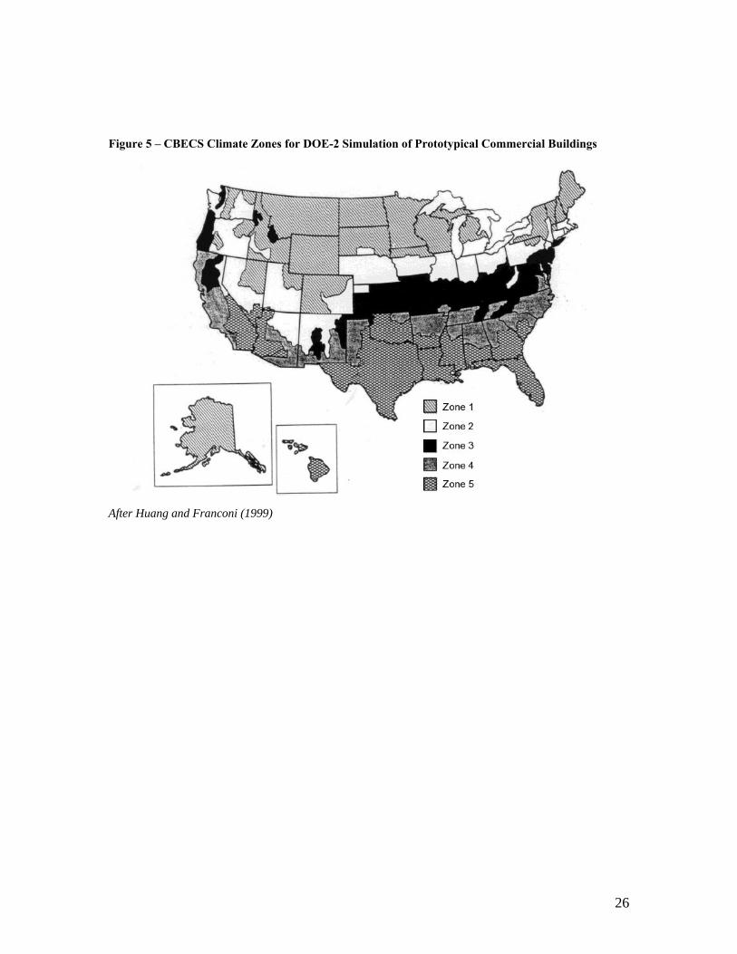
Figure 5 – CBECS Climate Zones for DOE-2 Simulation of Prototypical Commercial Buildings

After Huang and Franconi (1999)

26

Appendix C – Window Technology Scenario Assumptions Residential Sales Scenario Assumed window properties are presented in Table 14 and were determined as follows. First, we used market survey data to estimate the market shares of dominant window products (Ducker Research Company 2004). Next, we estimated average U-factor and SHGC for typical windows products in each category. We used the following simplifying assumptions: • All single pane windows use aluminum frames. • 75% of double pane (clear) windows have wood/vinyl frames, 25% have aluminum

frames. • All Double Pane Low-e windows have wood/vinyl frames and low-moderate solar

heat gain. • Triple pane windows have high-performance wood/vinyl frames and moderate solar

heat gain. Based on these assumptions, we used a database of currently available products to estimate typical window properties for each category (Carmody et al. 2000). Finally, we calculated sales-weighted average U-factor and SHGC for current residential window sales. Table 14 - Assumed Properties of Residential Window Sales

Window Type Percent of Sales U – Factor Btu / (hr-ft²-°F)

SHGC

Single Pane, Clear Glass 4% 1.16 0.76 Double Pane, Clear Glass 40% 0.54 0.56 Double Pane, Low-e Glass 54% 0.35 0.35 Triple Pane, Low-e Glass 2% 0.20 0.40

Average Properties 0.46 0.45

Residential Energy Star Scenario US EPA/DOE’s Energy Star program specifies minimum window energy performance standards for windows carrying the Energy Star label. Requirements are specified separately for four climate zones (Figure 6). Table 15 presents Energy Star Window product requirements and assumed window properties by climate zone. We assume that windows just meet the Energy Star specification for U-value. Since low-solar heat gain glazings are now the dominant low-e product in the U.S. (Ducker Research Company 2004), we assume that all low-E windows sold in the US have SHGC = 0.40, which is required of Energy Star products in the Southern U.S. As can be seen in Figure 3 and Figure 6, Energy Star climate zones do not overlap perfectly with the climate zones devised by Huang et al. for the simulation of residential prototypical buildings. We mapped each of Huang’s climate zones to one Energy Star climate zone, as presented in Table 16.

27

Figure 6 - Energy Star Windows Climate Zones

Table 15 - Energy Star Window Assumptions

Energy Star Specification Requirements

Window Properties as Simulated

Energy Star Climate Zone

U – Factor Btu / (hr-ft²-°F)

SHGC U – Factor Btu / (hr-ft²-°F)

SHGC

Northern ≤ 0.35 Any 0.35 0.40 North/Central ≤ 0.40 ≤ 0.55 0.4 0.40 South/Central ≤ 0.40 ≤ 0.40 0.4 0.40

Southern ≤ 0.65 ≤ 0.40 0.65 0.40 Table 16 - Energy Star Climate Zones Energy Star Climate Zone Corresponding Climate

Zones Used by Huang et al. (see Appendix A)

Northern 1,2,3,4,5,14,15,18 North/Central 6,7,10,16 South/Central 8,11,12,17,19,20

Southern 9,13 Residential Mixed Triple, Dynamic Scenario The Mixed Triple, Dynamic scenario considers a regionally optimized deployment of windows from the Dynamic Low-e and Triple Pane Low-e scenarios, as described in the main text. Specifically, we assumed that windows from the Triple Pane Low-e scenario

28

were installed in the climate zones simulated by Huang et al. corresponding to the Northern and North/Central Energy Star Climate Zones. Dynamic Low-e Scenario were assumed to have been installed in the Southern and South/Central Energy Star Climate Zones. Commercial Sales Scenario Assumed window properties for the commercial sales scenario are presented in Table 14 and were determined as follows. First, we used market survey data to estimate the market shares of dominant window glazing types (Ducker Research Company 2004). Next, we assumed that all commercial glazings were installed in aluminum curtain wall frames, and assumed typical ASHRAE U-factor and SHGC for this type of installation (ASHRAE 2005)10. Based on these assumptions, we calculated sales-weighted average U-Factor and SHGC for commercial windows sales. Table 17 - Assumed Properties of Commercial Window Sales

Window Type Percent of

Sales U – Factor

Btu / (hr-ft²-°F) SHGC

Single Pane, Clear Glass 11% 1.16 0.74 Double Pane, Clear Glass 30% 0.62 0.63

Double Pane, Tinted Glass 6% 0.65 0.13 Double Pane, Reflective Glass 20% 0.62 0.46

Double Pane, Low-e Glass 30% 0.51 0.34 Triple Pane, Low-e Glass 3% 0.51 0.34

Average Properties 100% 0.64 0.48

10 This assumption provides a conservative estimate of window savings from this scenario; if some glazings are installed in more energy-efficient frames, energy savings would be higher.

29

Appendix D – Complete Residential Results Heating Loads

Number of Buildings (Thousands, 1993)

U Factor SHGC Window

SolarWindow

Cond Infiltration Other Loads Total Loads Number of Buildings

(Thousands, 2001) U Factor SHGC Window Solar Window Cond

Window Infiltration

Non-Window Infiltration

Other Loads Total Loads

1 Before 1950 1217.5 0.55 0.67 7.65 -18.3 -34.15 -38.11 -82.91 1175.9 0.55 0.65 7.16 -17.57 -4.95 -28.04 -39.64 -83.031 1950-1979 1031.1 0.72 0.72 8.04 -31.59 -32.72 -34.48 -90.75 1292.0 0.61 0.66 9.21 -33.55 -6.15 -34.85 -20.24 -85.591 1980-1989 326 0.72 0.72 1.69 -6.36 -7.95 -8 -20.62 369.2 0.61 0.66 1.75 -6.10 -1.35 -7.65 -6.33 -19.681 After 1989 135.2 0.50 0.61 0.04 -2.41 -3.04 -1.64 -7.05 226.4 0.46 0.59 0.07 -3.74 -0.76 -4.33 2.01 -6.762 Before 1950 2360.9 0.55 0.67 12.34 -30.28 -59.96 -64.79 -142.69 2132.7 0.55 0.65 10.80 -27.19 -8.12 -46.04 -72.32 -142.872 1950-1979 3477.5 0.72 0.72 19.83 -85.15 -94 -101.5 -260.82 2807.8 0.61 0.66 14.63 -58.25 -11.38 -64.51 -132.18 -251.692 1980-1989 788.8 0.72 0.72 2.95 -13.47 -19.04 -8.93 -38.49 637.1 0.61 0.66 2.18 -9.20 -2.31 -13.07 -14.61 -37.022 After 1989 212.6 0.50 0.61 0 -3.34 -4.78 -2.26 -10.38 536.4 0.46 0.59 0.00 -7.81 -1.81 -10.25 10.11 -9.763 Before 1950 961.6 0.55 0.67 7.23 -17.71 -30.31 -38.31 -79.1 3660.2 0.55 0.65 26.68 -67.01 -17.31 -98.07 76.16 -79.543 1950-1979 1238.4 0.72 0.72 4.75 -24.12 -23.72 -35.75 -78.84 4153.9 0.61 0.66 14.56 -68.63 -11.93 -67.63 65.69 -67.943 1980-1989 355.9 0.72 0.72 2 -7.62 -8.77 -10.04 -24.43 1240.3 0.61 0.66 6.37 -22.44 -4.58 -25.98 25.72 -20.923 After 1989 203.8 0.50 0.61 0.08 -4.19 -4.87 -3.19 -12.17 1368.8 0.46 0.59 0.52 -26.07 -4.91 -27.80 48.14 -10.124 Before 1950 3409.1 0.55 0.67 25.57 -62.6 -107.15 -135.48 -279.66 0.0 0.55 0.65 0.00 0.00 0.00 0.00 -279.66 -279.664 1950-1979 3757 0.72 0.72 14.71 -74.78 -73.54 -110.83 -244.44 0.0 0.61 0.66 0.00 0.00 0.00 0.00 -244.44 -244.444 1980-1989 591.8 0.72 0.72 3.46 -13.21 -15.2 -17.39 -42.34 0.0 0.61 0.66 0.00 0.00 0.00 0.00 -42.34 -42.344 After 1989 276.4 0.50 0.61 0.11 -5.96 -6.93 -4.55 -17.33 0.0 0.46 0.59 0.00 0.00 0.00 0.00 -17.33 -17.335 Before 1950 1414.6 0.55 0.67 10.76 -31.53 -52.1 -71.88 -144.75 852.4 0.55 0.65 6.28 -18.89 -4.71 -26.69 -100.84 -144.835 1950-1979 772 0.72 0.72 2.15 -16.02 -15.45 -26.75 -56.07 511.6 0.61 0.66 1.30 -9.00 -1.54 -8.70 -36.64 -54.585 1980-1989 47.3 0.72 0.72 0.23 -1.09 -1.41 -1.22 -3.49 148.8 0.61 0.66 0.66 -2.90 -0.67 -3.77 3.65 -3.025 After 1989 103.6 0.50 0.61 -0.06 -2.28 -2.1 -1.64 -6.08 49.4 0.46 0.59 -0.03 -1.01 -0.15 -0.85 -3.96 -6.006 Before 1950 1051.2 0.55 0.67 6.87 -13.92 -20.94 -27.32 -55.31 1287.7 0.55 0.65 8.16 -16.95 -3.85 -21.80 -21.02 -55.476 1950-1979 901.4 0.72 0.72 2.93 -11.03 -9.83 -14.83 -32.76 1428.9 0.61 0.66 4.24 -14.82 -2.34 -13.25 -4.34 -30.506 1980-1989 350.6 0.72 0.72 2.23 -6.24 -6.5 -7.66 -18.17 433.9 0.61 0.66 2.52 -6.53 -1.21 -6.84 -5.16 -17.216 After 1989 196.6 0.50 0.61 0.32 -2.93 -3.07 -1.87 -7.55 314.0 0.46 0.59 0.50 -4.34 -0.74 -4.17 1.52 -7.227 Before 1950 1655.3 1.02 0.75 12.24 -32.18 -30.52 -44.48 -94.94 624.7 0.94 0.72 4.40 -11.14 -1.73 -9.79 -75.90 -94.167 1950-1979 3556 1.28 0.81 34.47 -113.07 -70.39 -101.99 -250.98 1118.6 1.06 0.73 9.76 -29.25 -3.32 -18.82 -204.11 -245.757 1980-1989 1058.5 0.72 0.72 5.42 -17.25 -17.03 -10.33 -39.19 436.2 0.61 0.66 2.04 -6.02 -1.05 -5.96 -27.30 -38.297 After 1989 551.5 0.50 0.61 0.72 -8.61 -9.15 -5.1 -22.14 394.8 0.46 0.59 0.50 -5.71 -0.98 -5.57 -9.94 -21.708 Before 1950 166.3 1.02 0.76 0.65 -2.19 -2.36 -2.76 -6.66 1149.8 0.94 0.72 4.28 -13.88 -2.45 -13.87 20.31 -5.628 1950-1979 806.5 1.28 0.81 4.08 -16.31 -11.3 -9.17 -32.7 3125.4 1.06 0.73 14.23 -52.01 -6.57 -37.22 58.49 -23.098 1980-1989 189.9 0.72 0.72 0.83 -2.03 -2.13 -1.29 -4.62 1130.8 0.61 0.66 4.52 -10.22 -1.90 -10.78 15.21 -3.178 After 1989 585.4 0.66 0.68 2.54 -5.27 -6.3 -3.14 -12.17 1690.3 0.59 0.65 7.04 -13.75 -2.73 -15.46 13.90 -10.999 Before 1950 114.1 0.55 0.67 0.04 -0.11 -0.11 -0.13 -0.31 67.2 0.55 0.65 0.02 -0.06 -0.01 -0.06 -0.20 -0.319 1950-1979 924.1 0.72 0.72 0.41 -1.18 -0.74 -0.35 -1.86 1274.8 0.61 0.66 0.52 -1.38 -0.15 -0.87 0.22 -1.669 1980-1989 803.8 1.28 0.81 0.23 -0.57 -0.38 0.08 -0.64 929.8 1.06 0.73 0.24 -0.54 -0.07 -0.37 0.19 -0.559 After 1989 185.7 1.13 0.77 0.06 -0.13 -0.09 0.03 -0.13 441.0 0.98 0.72 0.13 -0.27 -0.03 -0.18 0.25 -0.10

10 Before 1950 1110.1 1.02 0.75 4.29 -14.43 -15.54 -18.23 -43.91 213.3 0.94 0.72 0.79 -2.54 -0.45 -2.54 -38.97 -43.7210 1950-1979 2023.3 1.28 0.81 10.08 -40.29 -27.93 -22.65 -80.79 246.5 1.06 0.73 1.11 -4.04 -0.51 -2.89 -73.71 -80.0410 1980-1989 540.1 0.72 0.72 2.3 -5.59 -5.87 -3.61 -12.77 194.3 0.61 0.66 0.76 -1.70 -0.32 -1.80 -9.47 -12.5310 After 1989 259.5 0.50 0.61 1.24 -2.57 -3.08 -1.53 -5.94 251.5 0.46 0.59 1.17 -2.31 -0.45 -2.54 -1.67 -5.7911 Before 1950 62.9 1.02 0.76 0.15 -0.37 -0.37 -0.51 -1.1 975.2 0.94 0.72 2.21 -5.26 -0.86 -4.88 8.05 -0.7411 1950-1979 380.6 1.28 0.81 1.28 -3.15 -1.91 -1.05 -4.83 1600.6 1.06 0.73 4.84 -10.90 -1.20 -6.83 11.07 -3.0211 1980-1989 104.9 0.72 0.72 0.31 -0.72 -0.5 -0.17 -1.08 700.7 0.61 0.66 1.89 -4.07 -0.50 -2.84 5.00 -0.5111 After 1989 23.8 0.66 0.68 0.08 -0.17 -0.13 -0.01 -0.23 643.7 0.59 0.65 2.08 -4.15 -0.53 -2.99 5.72 0.1312 Before 1950 1449.4 1.02 0.76 5.2 -12.34 -13.65 -18.92 -39.71 1266.9 0.94 0.72 4.33 -9.89 -1.79 -10.14 -21.54 -39.0312 1950-1979 3268.1 1.28 0.81 17 -42.72 -28.18 -21.88 -75.78 2015.3 1.06 0.73 9.43 -21.69 -2.61 -14.77 -42.54 -72.1812 1980-1989 1424.8 1.28 0.81 6.05 -14.89 -11.29 -4.36 -24.49 704.7 1.06 0.73 2.69 -6.06 -0.84 -4.75 -14.53 -23.4812 After 1989 427.5 1.13 0.77 2.11 -4.83 -3.84 -1.46 -8.02 681.7 0.98 0.72 3.18 -6.72 -0.92 -5.21 2.44 -7.2213 Before 1950 103.5 1.02 0.76 0.25 -0.6 -0.59 -0.83 -1.77 466.1 0.94 0.72 1.07 -2.48 -0.40 -2.26 2.46 -1.6013 1950-1979 346.9 1.28 0.81 1.17 -2.87 -1.75 -0.95 -4.4 1816.0 1.06 0.73 5.51 -12.37 -1.37 -7.79 13.66 -2.3613 1980-1989 180.2 1.28 0.81 0.54 -1.25 -0.87 -0.3 -1.88 516.6 1.06 0.73 1.39 -2.95 -0.37 -2.12 2.65 -1.4014 Before 1950 383.6 0.55 0.67 3.06 -6.65 -5.69 -12.54 -21.82 270.9 0.55 0.65 2.09 -4.67 -0.60 -3.42 -15.27 -21.8614 1950-1979 586.3 0.72 0.72 4.56 -11.93 -6.92 -9.78 -24.07 392.6 0.61 0.66 2.79 -6.77 -0.69 -3.94 -14.50 -23.1214 1980-1989 142.7 0.72 0.72 1.54 -2.92 -2.44 -2.42 -6.24 11.9 0.61 0.66 0.12 -0.21 -0.03 -0.17 -5.92 -6.2114 After 1989 94.1 0.50 0.61 0.58 -1.83 -1.55 -1.32 -4.12 51.2 0.46 0.59 0.31 -0.92 -0.13 -0.72 -2.60 -4.0515 Before 1950 202.6 1.02 0.75 1.56 -3.4 -2.91 -6.41 -11.16 326.1 0.94 0.72 2.39 -5.02 -0.70 -3.98 -3.51 -10.8315 1950-1979 535.1 1.28 0.81 3.84 -10.05 -5.83 -8.22 -20.26 626.0 1.06 0.73 4.04 -9.67 -1.02 -5.80 -6.17 -18.6215 1980-1989 34.6 0.72 0.72 0.32 -0.61 -0.51 -0.5 -1.3 211.0 0.61 0.66 1.78 -3.14 -0.47 -2.64 3.58 -0.8915 After 1989 75.8 0.50 0.61 0.39 -1.24 -1.05 -0.89 -2.79 575.6 0.46 0.59 2.89 -8.72 -1.20 -6.78 11.64 -2.1716 Before 1950 70.4 1.02 0.75 0.5 -0.91 -0.74 -1.59 -2.74 64.7 0.94 0.72 0.44 -0.77 -0.10 -0.58 -1.68 -2.6916 1950-1979 335.5 1.28 0.81 2.26 -4.73 -2.67 -3.33 -8.47 181.7 1.06 0.73 1.10 -2.11 -0.22 -1.23 -5.69 -8.1416 1980-1989 74.3 0.72 0.72 0.39 -0.67 -0.67 -0.51 -1.46 0.0 0.61 0.66 0.00 0.00 0.00 0.00 -1.46 -1.4616 After 1989 28.5 0.50 0.61 0.1 -0.26 -0.28 -0.22 -0.66 13.0 0.46 0.59 0.04 -0.11 -0.02 -0.11 -0.46 -0.6517 Before 1950 115.3 1.02 0.75 0.24 -0.44 -0.34 -0.74 -1.28 154.7 0.94 0.72 0.31 -0.54 -0.07 -0.39 -0.56 -1.2517 1950-1979 482.8 1.28 0.81 1.18 -2.03 -1.17 -0.93 -2.95 814.4 1.06 0.73 1.79 -2.82 -0.30 -1.68 0.46 -2.5417 1980-1989 100.3 0.72 0.72 0.17 -0.25 -0.25 -0.1 -0.43 179.8 0.61 0.66 0.28 -0.38 -0.07 -0.38 0.16 -0.3918 Before 1950 997.4 0.55 0.67 4.42 -16.96 -28.53 -29.92 -70.99 432.7 0.55 0.65 1.86 -7.31 -1.86 -10.52 -53.17 -71.0018 1950-1979 966.9 0.72 0.72 3.6 -23.37 -22 -17.99 -59.76 1214.8 0.61 0.66 4.13 -24.90 -4.15 -23.49 -7.28 -55.6918 1980-1989 531.7 0.72 0.72 3.08 -13.82 -9.44 -2.6 -22.78 308.3 0.61 0.66 1.63 -6.79 -0.82 -4.65 -11.08 -21.7118 After 1989 205.6 0.50 0.61 -0.01 -5.05 -3.65 -0.38 -9.09 398.7 0.46 0.59 -0.02 -9.09 -1.06 -6.02 7.80 -8.3919 Before 1950 690 1.02 0.76 7 -12.44 -12.43 -18.32 -36.19 494.2 0.94 0.72 4.77 -8.17 -1.34 -7.57 -23.39 -35.6919 1950-1979 1642.4 1.28 0.81 15.69 -30.44 -19.28 -25.11 -59.14 1537.4 1.06 0.73 13.22 -23.45 -2.71 -15.34 -27.29 -55.5619 1980-1989 482.2 0.72 0.72 6.65 -6.69 -4.85 -5.04 -9.93 284.1 0.61 0.66 3.58 -3.34 -0.43 -2.43 -7.05 -9.6719 After 1989 75.9 0.66 0.68 1.05 -0.95 -0.77 -0.53 -1.2 431.3 0.59 0.65 5.72 -4.88 -0.66 -3.72 2.61 -0.9220 Before 1950 592 1.02 0.76 2.91 -4.67 -4.01 -7.48 -13.25 927.0 0.94 0.72 4.34 -6.70 -0.94 -5.34 -4.21 -12.8620 1950-1979 1961.1 1.28 0.81 11.13 -18.78 -10.39 -15.95 -33.99 2110.2 1.06 0.73 10.78 -16.63 -1.68 -9.50 -14.58 -31.6120 1980-1989 283.4 0.72 0.72 2.07 -1.85 -1.23 -1.03 -2.04 287.4 0.61 0.66 1.92 -1.59 -0.19 -1.06 -1.02 -1.9320 After 1989 56.5 0.66 0.68 0.51 -0.4 -0.3 -0.19 -0.38 552.9 0.59 0.65 4.79 -3.54 -0.44 -2.50 1.48 -0.21

Number of Buildings (Thousands, 1993)

U Factor SHGC Window

SolarWindow

Cond Infiltration Other Loads Total Loads Number of Buildings

(Thousands, 2001) U Factor SHGC Window Solar Window Cond

Window Infiltration

Non-Window Infiltration

Other Loads Total Loads

Total 59230.60 0.85 0.73 328.41 -1015.16 -1053.43 -1217.55 -2957.73 62156.65 0.74 0.68 284.81 -825.57 -146.74 -831.50 -1347.49 -2866.49Percentage of Total Loads -11% 34% 36% 41% 100% -10% 29% 5% 29% 47% 100%

Windows 15% of total infiltration Window Total -844.76 Trillion BTU Loads Window Total -687.50 Trillion BTU LoadsWindow % of Total 29% Window % of Total 24%

Total Quads Heat 6.90 QuadsTotal Quads Window Heat 1.65 Quads

Window Properties Total Building Heating Loads (Trillion BTU/yr) Window Properties Total Building Cooling Loads (Trillion BTU/yr)

Climate Zone Year Made

1991 Properties Estimated by Huang, Hanford, et al (1999) 2001 Updated Window Stock Estimates (Apte and Arasteh, 2006)Window Properties Total Building Heating Loads (Trillion BTU/yr) Window Properties Total Building Cooling Loads (Trillion BTU/yr)

Totals/Averages

30

Cooling Loads

Number of Buildings (Thousands, 1993)

U Factor SHGC Window

SolarWindow

Cond Infiltration Other Loads Total Loads Number of Buildings

(Thousands, 2001) U Factor SHGC Window Solar

Window Cond

Window Infiltration

Non-Window Infiltration

Other Loads

Total Loads

1 Before 1950 1217.5 0.55 0.67 2.04 -0.1 -20.21 -17.6 -82.91 1175.9 0.55 0.65 -0.10 1.91 0.10 0.57 2.06 4.541 1950-1979 1031.1 0.72 0.72 8.04 -31.59 -32.72 -34.48 -90.75 1292.0 0.61 0.66 -0.07 3.21 0.13 0.73 0.44 4.441 1980-1989 326 0.72 0.72 1.69 -6.36 -7.95 -8 -20.62 369.2 0.61 0.66 0.01 0.61 0.03 0.17 0.27 1.091 After 1989 135.2 0.50 0.61 0.04 -2.41 -3.04 -1.64 -7.05 226.4 0.46 0.59 0.02 0.41 0.02 0.10 -0.04 0.502 Before 1950 2360.9 0.55 0.67 12.34 -30.28 -59.96 -64.79 -142.69 2132.7 0.55 0.65 -0.26 3.99 0.27 1.52 6.98 12.502 1950-1979 3477.5 0.72 0.72 19.83 -85.15 -94 -101.5 -260.82 2807.8 0.61 0.66 0.04 11.25 0.58 3.26 16.20 31.322 1980-1989 788.8 0.72 0.72 2.95 -13.47 -19.04 -8.93 -38.49 637.1 0.61 0.66 -0.02 1.71 0.10 0.59 2.94 5.322 After 1989 212.6 0.50 0.61 0 -3.34 -4.78 -2.26 -10.38 536.4 0.46 0.59 0.07 1.01 0.06 0.34 -0.51 0.973 Before 1950 961.6 0.55 0.67 7.23 -17.71 -30.31 -38.31 -79.1 3660.2 0.55 0.65 -0.61 10.70 0.65 3.69 -7.59 6.853 1950-1979 1238.4 0.72 0.72 4.75 -24.12 -23.72 -35.75 -78.84 4153.9 0.61 0.66 0.40 9.53 0.53 2.99 -7.71 5.743 1980-1989 355.9 0.72 0.72 2 -7.62 -8.77 -10.04 -24.43 1240.3 0.61 0.66 0.80 4.33 0.24 1.33 -4.28 2.423 After 1989 203.8 0.50 0.61 0.08 -4.19 -4.87 -3.19 -12.17 1368.8 0.46 0.59 0.37 6.29 0.31 1.77 -6.85 1.894 Before 1950 3409.1 0.55 0.67 25.57 -62.6 -107.15 -135.48 -279.66 0.0 0.55 0.65 0.00 0.00 0.00 0.00 28.89 28.894 1950-1979 3757 0.72 0.72 14.71 -74.78 -73.54 -110.83 -244.44 0.0 0.61 0.66 0.00 0.00 0.00 0.00 25.71 25.714 1980-1989 591.8 0.72 0.72 3.46 -13.21 -15.2 -17.39 -42.34 0.0 0.61 0.66 0.00 0.00 0.00 0.00 5.49 5.494 After 1989 276.4 0.50 0.61 0.11 -5.96 -6.93 -4.55 -17.33 0.0 0.46 0.59 0.00 0.00 0.00 0.00 2.48 2.485 Before 1950 1414.6 0.55 0.67 10.76 -31.53 -52.1 -71.88 -144.75 852.4 0.55 0.65 -0.16 3.24 0.18 1.00 7.78 12.045 1950-1979 772 0.72 0.72 2.15 -16.02 -15.45 -26.75 -56.07 511.6 0.61 0.66 0.06 1.17 0.06 0.35 2.40 4.045 1980-1989 47.3 0.72 0.72 0.23 -1.09 -1.41 -1.22 -3.49 148.8 0.61 0.66 0.00 0.46 0.02 0.13 -0.37 0.255 After 1989 103.6 0.50 0.61 -0.06 -2.28 -2.1 -1.64 -6.08 49.4 0.46 0.59 0.01 0.16 0.01 0.04 0.46 0.676 Before 1950 1051.2 0.55 0.67 6.87 -13.92 -20.94 -27.32 -55.31 1287.7 0.55 0.65 -0.19 9.94 0.88 4.99 8.76 24.386 1950-1979 901.4 0.72 0.72 2.93 -11.03 -9.83 -14.83 -32.76 1428.9 0.61 0.66 0.55 7.65 0.60 3.38 2.12 14.306 1980-1989 350.6 0.72 0.72 2.23 -6.24 -6.5 -7.66 -18.17 433.9 0.61 0.66 0.20 3.68 0.28 1.60 2.18 7.946 After 1989 196.6 0.50 0.61 0.32 -2.93 -3.07 -1.87 -7.55 314.0 0.46 0.59 0.27 2.79 0.19 1.07 0.05 4.377 Before 1950 1655.3 1.02 0.75 12.24 -32.18 -30.52 -44.48 -94.94 624.7 0.94 0.72 -0.14 3.37 0.22 1.22 20.48 25.157 1950-1979 3556 1.28 0.81 34.47 -113.07 -70.39 -101.99 -250.98 1118.6 1.06 0.73 0.32 9.78 0.45 2.57 62.28 75.417 1980-1989 1058.5 0.72 0.72 5.42 -17.25 -17.03 -10.33 -39.19 436.2 0.61 0.66 -0.10 2.91 0.13 0.75 13.53 17.237 After 1989 551.5 0.50 0.61 0.72 -8.61 -9.15 -5.1 -22.14 394.8 0.46 0.59 0.05 2.63 0.12 0.68 5.04 8.518 Before 1950 166.3 1.02 0.76 0.65 -2.19 -2.36 -2.76 -6.66 1149.8 0.94 0.72 -0.38 5.07 0.51 2.88 -5.00 3.088 1950-1979 806.5 1.28 0.81 4.08 -16.31 -11.3 -9.17 -32.7 3125.4 1.06 0.73 -0.38 18.27 1.46 8.30 -13.70 13.968 1980-1989 189.9 0.72 0.72 0.83 -2.03 -2.13 -1.29 -4.62 1130.8 0.61 0.66 -0.50 8.44 0.46 2.58 -7.95 3.028 After 1989 585.4 0.66 0.68 2.54 -5.27 -6.3 -3.14 -12.17 1690.3 0.59 0.65 -0.99 13.53 0.68 3.83 -6.60 10.449 Before 1950 114.1 0.55 0.67 0.04 -0.11 -0.11 -0.13 -0.31 67.2 0.55 0.65 -0.05 0.75 0.13 0.76 4.98 6.579 1950-1979 924.1 0.72 0.72 0.41 -1.18 -0.74 -0.35 -1.86 1274.8 0.61 0.66 0.91 17.12 2.30 13.05 16.16 49.549 1980-1989 803.8 1.28 0.81 0.23 -0.57 -0.38 0.08 -0.64 929.8 1.06 0.73 -0.40 11.26 1.28 7.28 14.58 34.009 After 1989 185.7 1.13 0.77 0.06 -0.13 -0.09 0.03 -0.13 441.0 0.98 0.72 -0.23 6.01 0.62 3.51 -2.23 7.69

10 Before 1950 1110.1 1.02 0.75 4.29 -14.43 -15.54 -18.23 -43.91 213.3 0.94 0.72 -0.07 0.93 0.09 0.52 20.11 21.5810 1950-1979 2023.3 1.28 0.81 10.08 -40.29 -27.93 -22.65 -80.79 246.5 1.06 0.73 -0.03 1.44 0.12 0.65 37.59 39.7810 1980-1989 540.1 0.72 0.72 2.3 -5.59 -5.87 -3.61 -12.77 194.3 0.61 0.66 -0.09 1.38 0.08 0.43 8.19 9.9910 After 1989 259.5 0.50 0.61 1.24 -2.57 -3.08 -1.53 -5.94 251.5 0.46 0.59 -0.15 2.00 0.10 0.56 2.18 4.6911 Before 1950 62.9 1.02 0.76 0.15 -0.37 -0.37 -0.51 -1.1 975.2 0.94 0.72 -0.57 6.79 1.02 5.80 -11.31 1.7311 1950-1979 380.6 1.28 0.81 1.28 -3.15 -1.91 -1.05 -4.83 1600.6 1.06 0.73 -0.87 17.56 1.70 9.62 -17.87 10.1411 1980-1989 104.9 0.72 0.72 0.31 -0.72 -0.5 -0.17 -1.08 700.7 0.61 0.66 0.00 5.68 0.62 3.52 -7.48 2.3411 After 1989 23.8 0.66 0.68 0.08 -0.17 -0.13 -0.01 -0.23 643.7 0.59 0.65 0.24 5.71 0.57 3.22 -9.40 0.3512 Before 1950 1449.4 1.02 0.76 5.2 -12.34 -13.65 -18.92 -39.71 1266.9 0.94 0.72 0.45 7.61 1.32 7.50 25.96 42.8512 1950-1979 3268.1 1.28 0.81 17 -42.72 -28.18 -21.88 -75.78 2015.3 1.06 0.73 2.63 18.03 2.22 12.60 61.81 97.2912 1980-1989 1424.8 1.28 0.81 6.05 -14.89 -11.29 -4.36 -24.49 704.7 1.06 0.73 0.98 5.14 0.66 3.76 26.13 36.6712 After 1989 427.5 1.13 0.77 2.11 -4.83 -3.84 -1.46 -8.02 681.7 0.98 0.72 1.15 5.49 0.69 3.90 -0.46 10.7813 Before 1950 103.5 1.02 0.76 0.25 -0.6 -0.59 -0.83 -1.77 466.1 0.94 0.72 -0.29 3.13 0.48 2.72 -2.97 3.0713 1950-1979 346.9 1.28 0.81 1.17 -2.87 -1.75 -0.95 -4.4 1816.0 1.06 0.73 -0.99 19.92 1.92 10.90 -22.92 8.8413 1980-1989 180.2 1.28 0.81 0.54 -1.25 -0.87 -0.3 -1.88 516.6 1.06 0.73 0.00 4.13 0.46 2.61 -2.72 4.4714 Before 1950 383.6 0.55 0.67 3.06 -6.65 -5.69 -12.54 -21.82 270.9 0.55 0.65 0.00 0.22 0.00 0.02 0.72 0.9614 1950-1979 586.3 0.72 0.72 4.56 -11.93 -6.92 -9.78 -24.07 392.6 0.61 0.66 0.02 0.24 0.01 0.03 0.51 0.8014 1980-1989 142.7 0.72 0.72 1.54 -2.92 -2.44 -2.42 -6.24 11.9 0.61 0.66 0.00 0.01 0.00 0.00 0.13 0.1414 After 1989 94.1 0.50 0.61 0.58 -1.83 -1.55 -1.32 -4.12 51.2 0.46 0.59 0.01 0.04 0.00 0.00 0.08 0.1315 Before 1950 202.6 1.02 0.75 1.56 -3.4 -2.91 -6.41 -11.16 326.1 0.94 0.72 0.00 0.31 0.01 0.04 0.24 0.5915 1950-1979 535.1 1.28 0.81 3.84 -10.05 -5.83 -8.22 -20.26 626.0 1.06 0.73 0.04 0.39 0.01 0.05 0.24 0.7315 1980-1989 34.6 0.72 0.72 0.32 -0.61 -0.51 -0.5 -1.3 211.0 0.61 0.66 0.00 0.11 0.00 0.00 -0.09 0.0215 After 1989 75.8 0.50 0.61 0.39 -1.24 -1.05 -0.89 -2.79 575.6 0.46 0.59 0.14 1.11 0.01 0.06 -1.08 0.2516 Before 1950 70.4 1.02 0.75 0.5 -0.91 -0.74 -1.59 -2.74 64.7 0.94 0.72 0.00 0.08 0.00 0.01 0.21 0.3016 1950-1979 335.5 1.28 0.81 2.26 -4.73 -2.67 -3.33 -8.47 181.7 1.06 0.73 0.01 0.26 0.00 0.02 0.91 1.2116 1980-1989 74.3 0.72 0.72 0.39 -0.67 -0.67 -0.51 -1.46 0.0 0.61 0.66 0.00 0.00 0.00 0.00 0.31 0.3116 After 1989 28.5 0.50 0.61 0.1 -0.26 -0.28 -0.22 -0.66 13.0 0.46 0.59 0.01 0.04 0.00 0.01 0.14 0.1917 Before 1950 115.3 1.02 0.75 0.24 -0.44 -0.34 -0.74 -1.28 154.7 0.94 0.72 0.09 0.40 0.04 0.25 0.71 1.4917 1950-1979 482.8 1.28 0.81 1.18 -2.03 -1.17 -0.93 -2.95 814.4 1.06 0.73 1.66 5.07 0.44 2.47 1.54 11.1817 1980-1989 100.3 0.72 0.72 0.17 -0.25 -0.25 -0.1 -0.43 179.8 0.61 0.66 0.46 1.38 0.16 0.93 0.35 3.2818 Before 1950 997.4 0.55 0.67 4.42 -16.96 -28.53 -29.92 -70.99 432.7 0.55 0.65 -0.01 0.10 0.00 0.00 0.59 0.6918 1950-1979 966.9 0.72 0.72 3.6 -23.37 -22 -17.99 -59.76 1214.8 0.61 0.66 -0.01 0.32 0.00 0.02 0.28 0.6118 1980-1989 531.7 0.72 0.72 3.08 -13.82 -9.44 -2.6 -22.78 308.3 0.61 0.66 -0.01 0.13 0.00 0.00 0.25 0.3718 After 1989 205.6 0.50 0.61 -0.01 -5.05 -3.65 -0.38 -9.09 398.7 0.46 0.59 0.00 0.28 0.00 0.00 -0.06 0.2219 Before 1950 690 1.02 0.76 7 -12.44 -12.43 -18.32 -36.19 494.2 0.94 0.72 -0.01 0.03 0.00 0.00 0.11 0.1319 1950-1979 1642.4 1.28 0.81 15.69 -30.44 -19.28 -25.11 -59.14 1537.4 1.06 0.73 -0.02 0.30 0.00 0.00 0.54 0.8319 1980-1989 482.2 0.72 0.72 6.65 -6.69 -4.85 -5.04 -9.93 284.1 0.61 0.66 0.00 0.09 0.00 0.01 0.16 0.2519 After 1989 75.9 0.66 0.68 1.05 -0.95 -0.77 -0.53 -1.2 431.3 0.59 0.65 0.00 0.16 0.00 0.00 -0.13 0.0320 Before 1950 592 1.02 0.76 2.91 -4.67 -4.01 -7.48 -13.25 927.0 0.94 0.72 -0.17 0.70 -0.03 -0.16 0.89 1.2320 1950-1979 1961.1 1.28 0.81 11.13 -18.78 -10.39 -15.95 -33.99 2110.2 1.06 0.73 -0.56 2.40 -0.13 -0.72 3.37 4.3620 1980-1989 283.4 0.72 0.72 2.07 -1.85 -1.23 -1.03 -2.04 287.4 0.61 0.66 -0.07 0.55 -0.02 -0.11 0.43 0.7820 After 1989 56.5 0.66 0.68 0.51 -0.4 -0.3 -0.19 -0.38 552.9 0.59 0.65 -0.18 0.85 -0.03 -0.17 -0.38 0.09

Number of Buildings (Thousands, 1993)

U Factor SHGC Window

SolarWindow

Cond Infiltration Other Loads Total Loads Number of Buildings

(Thousands, 2001) U Factor SHGC Window Solar

Window Cond

Window Infiltration

Non-Window Infiltration

Other Loads

Total Loads

Total 59230.60 0.85 0.73 322.80 -996.96 -1039.49 -1197.04 -2957.73 62156.65 0.74 0.68 3.28 303.66 26.14 148.11 307.27 788.46Percentage of Total Loads -11% 34% 35% 40% 100% 0% 39% 3% 19% 39% 100%

Windows 15% of total infiltration Window Total -830.08 Trillion BTU Loads Window Total 333.08 Trillion BTU LoadsWindow % of Total 28% Window % of Total 42%

Total Quads Cool 2.41 QuadsTotal Quads Window Cool 1.02 Quads

Window Properties Total Building Cooling Loads (Trillion BTU/yr) Window Properties Total Building Cooling Loads (Trillion BTU/yr)

Climate Zone Year Made

1993 Properties Estimated by Huang, Hanford, et al (1999) 2001 Updated Window Stock Estimates (Apte and Arasteh, 2006)Window Properties Total Building Cooling Loads (Trillion BTU/yr) Window Properties Total Building Cooling Loads (Trillion BTU/yr)

Totals/Averages

31

Appendix E – Complete Commercial Results Large and Small Office Buildings

Conditioned

32

Area, Million Square

Feet

U Factor SHGC Window Solar

Window Cond Infiltration Other

LoadsTotal Loads U Factor SHGC Window Solar Window

CondWindow

InfiltrationNon-Window

Infiltration Other Loads Total Loads

Large Office Minneapolis New heat 95.1 0.58 0.60 4.5 -11.9 -1.5 -0.5 -9.4 4.76 150.16 0.75 0.66 -1.1E+04 3.5E+03 -1.6E+02 -9.1E+02 -3.6E+02 -8.81E+03Large Office Minneapolis New cool 76.6 0.58 0.60 15.4 -5.2 -2 17.1 25.3 1.16 139.45 0.75 0.66 -1.1E+03 2.7E+03 -4.9E+01 -2.8E+02 2.8E+03 4.11E+03Large Office Chicago New heat 705 0.58 0.60 3.8 -8.7 -1.4 0.1 -6.2 5.56 1,068.46 0.75 0.66 -6.6E+04 2.5E+04 -1.2E+03 -7.1E+03 5.9E+02 -4.91E+04Large Office Chicago New cool 657.6 0.58 0.60 16.3 -5 -1.7 18.4 28 1.22 1,014.30 0.75 0.66 -7.9E+03 2.2E+04 -3.2E+02 -1.8E+03 2.3E+04 3.49E+04Large Office Washington New heat 556.4 0.59 0.61 2 -4.8 -0.5 0.1 -3.2 8.33 874.34 0.75 0.66 -4.4E+04 1.6E+04 -5.5E+02 -3.1E+03 7.3E+02 -3.14E+04Large Office Washington New cool 535.2 0.59 0.61 17.6 -4.9 -1.6 21 32.1 1.33 844.21 0.75 0.66 -7.0E+03 2.1E+04 -2.7E+02 -1.5E+03 2.4E+04 3.63E+04Large Office Los Angeles New heat 686.3 0.60 0.62 0.1 -0.2 0 0 -0.1 100.00 923.04 0.75 0.66 -2.3E+04 9.9E+03 0.0E+00 0.0E+00 0.0E+00 -1.33E+04Large Office Los Angeles New cool 701.9 0.60 0.62 31.5 -10.2 -1.3 25 45 1.33 925.16 0.75 0.66 -1.6E+04 4.2E+04 -2.4E+02 -1.4E+03 3.1E+04 5.50E+04Large Office Houston New heat 548.1 0.60 0.62 0.5 -1 -0.1 0.2 -0.4 25.00 451.33 0.75 0.66 -1.4E+04 6.0E+03 -1.7E+02 -9.6E+02 2.3E+03 -6.98E+03Large Office Houston New cool 548.7 0.60 0.62 24.8 -5.3 -1.4 26.4 44.5 1.43 499.24 0.75 0.66 -4.7E+03 1.9E+04 -1.5E+02 -8.5E+02 1.9E+04 3.20E+04

Large Office Minneapolis Old heat 239.4 0.69 0.70 4.9 -12.2 -1.5 -1.8 -10.6 4.17 304.38 0.75 0.66 -1.7E+04 5.9E+03 -2.9E+02 -1.6E+03 -2.3E+03 -1.50E+04Large Office Minneapolis Old cool 185.4 0.69 0.70 15.9 -4.8 -2.4 21.7 30.4 3.57 250.74 0.75 0.66 -4.6E+03 1.4E+04 -3.2E+02 -1.8E+03 1.9E+04 2.61E+04Large Office Chicago Old heat 1621.5 0.69 0.70 4 -8.9 -1.4 -0.7 -7 5.26 1,065.44 0.75 0.66 -5.4E+04 2.1E+04 -1.2E+03 -6.7E+03 -3.9E+03 -4.44E+04Large Office Chicago Old cool 1360.6 0.69 0.70 16.9 -4.8 -2.1 23.5 33.5 3.13 927.96 0.75 0.66 -1.5E+04 4.6E+04 -9.1E+02 -5.2E+03 6.8E+04 9.35E+04Large Office Washington Old heat 1745.3 0.71 0.68 1.9 -4.6 -0.5 -0.3 -3.5 8.33 1,556.73 0.75 0.66 -6.3E+04 2.4E+04 -9.7E+02 -5.5E+03 -3.9E+03 -4.99E+04Large Office Washington Old cool 1761.8 0.71 0.68 17.1 -4.6 -1.8 26.4 37.1 2.86 1,440.47 0.75 0.66 -2.0E+04 6.8E+04 -1.1E+03 -6.3E+03 1.1E+05 1.49E+05Large Office Los Angeles Old heat 996.2 0.72 0.67 0.1 -0.2 0 0 -0.1 100.00 771.60 0.75 0.66 -1.6E+04 7.6E+03 0.0E+00 0.0E+00 0.0E+00 -8.49E+03Large Office Los Angeles Old cool 983.2 0.72 0.67 26.2 -8.5 -1.3 31 47.4 2.27 785.41 0.75 0.66 -1.6E+04 4.6E+04 -3.5E+02 -2.0E+03 5.5E+04 8.33E+04Large Office Houston Old heat 428.8 0.72 0.67 0.5 -0.9 -0.1 0 -0.5 33.33 427.46 0.75 0.66 -1.3E+04 7.0E+03 -2.1E+02 -1.2E+03 0.0E+00 -7.77E+03Large Office Houston Old cool 324.7 0.72 0.67 20.5 -4.4 -1.5 33 47.6 2.13 507.98 0.75 0.66 -5.0E+03 2.2E+04 -2.4E+02 -1.4E+03 3.6E+04 5.09E+04

Small Office Minneapolis New heat 30.8 0.50 0.62 5.9 -10.3 -8.2 -10.8 -23.4 1.82 108.73 0.75 0.66 -3.0E+03 1.2E+03 -2.4E+02 -1.4E+03 -2.1E+03 -5.55E+03Small Office Minneapolis New cool 30.6 0.50 0.62 7.5 -1.1 -1 8.6 14 1.27 95.44 0.75 0.66 -2.0E+02 9.7E+02 -1.8E+01 -1.0E+02 1.0E+03 1.69E+03Small Office Chicago New heat 150.9 0.50 0.62 4.7 -7.6 -6.2 -6.6 -15.7 1.96 323.44 0.75 0.66 -7.2E+03 3.2E+03 -5.9E+02 -3.3E+03 -4.2E+03 -1.21E+04Small Office Chicago New cool 149.1 0.50 0.62 8.5 -1.3 -1.1 10.4 16.5 1.35 316.85 0.75 0.66 -8.3E+02 3.9E+03 -7.1E+01 -4.0E+02 4.5E+03 7.04E+03Small Office Washington New heat 214.3 0.56 0.63 3.7 -5.5 -5.2 -5.6 -12.6 1.85 359.68 0.75 0.66 -4.9E+03 2.6E+03 -5.2E+02 -2.9E+03 -3.7E+03 -9.54E+03Small Office Washington New cool 216 0.56 0.63 6.9 -0.8 -1 12.1 17.2 1.43 332.70 0.75 0.66 -5.1E+02 3.4E+03 -7.1E+01 -4.0E+02 5.8E+03 8.18E+03Small Office Los Angeles New heat 349.7 0.63 0.65 0.4 -0.4 -0.5 -0.3 -0.8 3.85 551.13 0.75 0.66 -1.0E+03 8.6E+02 -1.6E+02 -9.0E+02 -6.4E+02 -1.84E+03Small Office Los Angeles New cool 344.5 0.63 0.65 8.7 -1.3 -1.3 13.6 19.7 1.52 537.85 0.75 0.66 -1.3E+03 7.2E+03 -1.6E+02 -9.0E+02 1.1E+04 1.59E+04Small Office Houston New heat 276.7 0.63 0.65 1.5 -1.6 -1.7 -0.8 -2.6 2.27 174.64 0.75 0.66 -7.5E+02 6.0E+02 -1.0E+02 -5.7E+02 -3.2E+02 -1.14E+03Small Office Houston New cool 272.3 0.63 0.65 8.4 -0.6 -1 17.6 24.4 1.54 195.93 0.75 0.66 -2.1E+02 2.6E+03 -4.5E+01 -2.6E+02 5.3E+03 7.35E+03

Small Office Minneapolis Old heat 319.4 0.57 0.69 7.7 -14.6 -18.1 -25 1.85 171.87 0.75 0.66 -6.1E+03 2.4E+03 -3.5E+02 -2.0E+03 -3.4E+03 -9.54E+03Small Office Minneapolis Old cool 265.6 0.57 0.69 13 -2.4 -1.4 10.8 20 1.69 151.66 0.75 0.66 -8.1E+02 3.2E+03 -5.4E+01 -3.1E+02 2.8E+03 4.81E+03Small Office Chicago Old heat 661.8 0.57 0.69 5.7 -10.2 -5.3 -6.6 -16.4 1.96 315.55 0.75 0.66 -8.3E+03 3.4E+03 -4.9E+02 -2.8E+03 -4.1E+03 -1.23E+04Small Office Chicago Old cool 582.7 0.57 0.69 14.6 -2.7 -1.5 12.9 23.3 1.72 280.28 0.75 0.66 -1.7E+03 6.8E+03 -1.1E+02 -6.2E+02 6.2E+03 1.06E+04Small Office Washington Old heat 536.6 0.65 0.70 5.9 -8.7 -4.3 -3.1 -10.2 2.08 579.45 0.75 0.66 -1.2E+04 6.7E+03 -7.8E+02 -4.4E+03 -3.7E+03 -1.44E+04Small Office Washington Old cool 473.1 0.65 0.70 16.5 -3.3 -1.9 16.1 27.4 1.79 435.39 0.75 0.66 -3.0E+03 1.2E+04 -2.2E+02 -1.3E+03 1.3E+04 2.02E+04Small Office Los Angeles Old heat 591.4 0.75 0.71 0.3 -0.4 -0.2 -0.2 -0.5 11.11 530.93 0.75 0.66 -2.4E+03 1.6E+03 -1.8E+02 -1.0E+03 -1.2E+03 -3.09E+03Small Office Los Angeles Old cool 592.6 0.75 0.71 25 -5.4 -2.8 20 36.8 1.75 464.95 0.75 0.66 -4.4E+03 1.9E+04 -3.4E+02 -1.9E+03 1.6E+04 2.85E+04Small Office Houston Old heat 525.8 0.75 0.71 1.3 -1.7 -0.9 -0.3 -1.6 4.35 293.03 0.75 0.66 -2.2E+03 1.5E+03 -1.7E+02 -9.7E+02 -3.8E+02 -2.17E+03Small Office Houston Old cool 524.1 0.75 0.71 20 -1.9 -1.4 23.9 40.6 1.72 291.14 0.75 0.66 -9.6E+02 9.3E+03 -1.1E+02 -6.0E+02 1.2E+04 1.96E+04Large Office Total Total heat 7622.1 7,592.95 -3.22E+05 1.26E+05 -4.77E+03 -2.70E+04 -6.88E+03 -2.35E+05Large Office Total Total cool 7135.7 7,334.92 -9.70E+04 3.03E+05 -3.96E+03 -2.25E+04 3.86E+05 5.65E+05Small Office Total Total heat 3657.4 3,408.44 -4.81E+04 2.41E+04 -3.59E+03 -2.03E+04 -2.38E+04 -7.17E+04Small Office Total Total cool 3450.6 3,102.20 -1.39E+04 6.82E+04 -1.20E+03 -6.78E+03 7.75E+04 1.24E+05

1999 Updated Window Stock Estimates (Apte and Arasteh, 2006)Window Properties Total Building Energy Consumption (Trillion BTU/yr)Conditioned

Area, Million Square

Feet

Building Type Vintage

1991 Properties Estimated by Huang and Franconi (1999)System Efficiency

Factor (Primary kBtu

Energy Consumption / kBtu Load)

Climate ZoneSpace

Conditioning Mode

Window Properties Building HVAC Load Intensity (kBtu/ft²/yr)

Large and Small Retail Buildings

Conditioned

33

Area, Million Square

Feet

U Factor SHGC Window Solar

Window Cond Infiltration Other

LoadsTotal Loads U Factor SHGC Window Solar Window

CondWindow

InfiltrationNon-Window

Infiltration Other Loads Total Loads

Large Retail Minneapolis New heat 188.3 0.58 0.64 1.5 -3.8 -5.6 1.4 -6.5 5.00 91.91 0.75 0.66 -2.2E+03 7.1E+02 -3.9E+02 -2.2E+03 6.4E+02 -3.46E+03Large Retail Minneapolis New cool 177 0.58 0.64 4.6 -1.6 -1.8 18.2 19.4 1.39 76.15 0.75 0.66 -2.2E+02 5.0E+02 -2.9E+01 -1.6E+02 1.9E+03 2.02E+03Large Retail Chicago New heat 745.6 0.58 0.64 0.9 -2.1 -3.4 1.3 -3.3 7.14 457.24 0.75 0.66 -8.8E+03 3.0E+03 -1.7E+03 -9.4E+03 4.2E+03 -1.26E+04Large Retail Chicago New cool 546.2 0.58 0.64 4.6 -1.2 -1.1 20.5 22.8 1.43 422.59 0.75 0.66 -9.3E+02 2.8E+03 -1.0E+02 -5.6E+02 1.2E+04 1.36E+04Large Retail Washington New heat 178.5 0.59 0.65 0.2 -0.5 -1 0.2 -1.1 14.29 481.10 0.75 0.66 -4.4E+03 1.4E+03 -1.0E+03 -5.8E+03 1.4E+03 -8.46E+03Large Retail Washington New cool 173.6 0.59 0.65 4.8 -0.7 -0.1 23.1 27.1 1.52 466.90 0.75 0.66 -6.3E+02 3.4E+03 -1.1E+01 -6.0E+01 1.6E+04 1.91E+04Large Retail Los Angeles New heat 230.6 0.60 0.66 0 0 0 0 0 - 784.11 0.75 0.66 0.0E+00 0.0E+00 0.0E+00 0.0E+00 0.0E+00 0.00E+00Large Retail Los Angeles New cool 201.3 0.60 0.66 8.4 -2.3 -2.9 32.9 36.1 1.33 789.88 0.75 0.66 -3.0E+03 8.8E+03 -4.6E+02 -2.6E+03 3.5E+04 3.74E+04Large Retail Houston New heat 409.4 0.60 0.66 0 0 0 0 0 100.00 568.30 0.75 0.66 0.0E+00 0.0E+00 0.0E+00 0.0E+00 0.0E+00 0.00E+00Large Retail Houston New cool 368.4 0.60 0.66 6.5 -0.9 -1.1 34.5 39 1.52 647.95 0.75 0.66 -1.1E+03 6.4E+03 -1.6E+02 -9.2E+02 3.4E+04 3.81E+04

Large Retail Minneapolis Old heat 345.9 0.65 0.68 2.3 -5.1 -8.8 2.5 -9.1 6.25 147.66 0.75 0.66 -5.4E+03 2.1E+03 -1.2E+03 -6.9E+03 2.3E+03 -9.19E+03Large Retail Minneapolis Old cool 243.8 0.65 0.68 4.8 -2 -3.2 18.1 17.7 2.86 121.54 0.75 0.66 -8.0E+02 1.6E+03 -1.7E+02 -9.4E+02 6.3E+03 5.99E+03Large Retail Chicago Old heat 806.8 0.65 0.68 1.5 -3.1 -5.7 2.2 -5.1 9.09 442.88 0.75 0.66 -1.4E+04 5.9E+03 -3.4E+03 -2.0E+04 8.9E+03 -2.26E+04Large Retail Chicago Old cool 381.9 0.65 0.68 4.7 -1.3 -2 19.5 20.9 2.50 378.16 0.75 0.66 -1.4E+03 4.3E+03 -2.8E+02 -1.6E+03 1.8E+04 1.94E+04Large Retail Washington Old heat 1162 0.68 0.68 0.3 -0.8 -1.9 0.7 -1.7 20.00 480.26 0.75 0.66 -8.4E+03 2.8E+03 -2.7E+03 -1.6E+04 6.7E+03 -1.72E+04Large Retail Washington Old cool 924.6 0.68 0.68 4.5 -0.5 -0.2 21.5 25.3 2.22 445.90 0.75 0.66 -5.4E+02 4.3E+03 -3.0E+01 -1.7E+02 2.1E+04 2.49E+04Large Retail Los Angeles Old heat 752.3 0.72 0.69 0 0 0 0 0 - 432.25 0.75 0.66 0.0E+00 0.0E+00 0.0E+00 0.0E+00 0.0E+00 0.00E+00Large Retail Los Angeles Old cool 686.4 0.72 0.69 8.7 -2.5 -4.5 32.7 34.4 1.72 441.14 0.75 0.66 -2.0E+03 6.4E+03 -5.1E+02 -2.9E+03 2.5E+04 2.58E+04Large Retail Houston Old heat 477.3 0.72 0.69 0 0 -0.1 0 -0.1 100.00 313.82 0.75 0.66 0.0E+00 0.0E+00 -4.7E+02 -2.7E+03 0.0E+00 -3.14E+03Large Retail Houston Old cool 412.3 0.72 0.69 6.6 -0.9 -1.8 33.4 37.3 1.72 398.25 0.75 0.66 -6.4E+02 4.4E+03 -1.9E+02 -1.1E+03 2.3E+04 2.54E+04

Small Retail Minneapolis New heat 71.5 0.58 0.74 4.3 -11.2 -9.4 -13.6 -29.9 1.72 106.89 0.75 0.66 -2.6E+03 7.1E+02 -2.6E+02 -1.5E+03 -2.5E+03 -6.18E+03Small Retail Minneapolis New cool 26.2 0.58 0.74 7.5 -1.2 -1 10.4 15.7 1.64 52.68 0.75 0.66 -1.3E+02 5.8E+02 -1.3E+01 -7.3E+01 9.0E+02 1.26E+03Small Retail Chicago New heat 189.1 0.58 0.74 3.5 -8.1 -7.1 -8.2 -19.9 1.75 262.51 0.75 0.66 -4.8E+03 1.4E+03 -4.9E+02 -2.8E+03 -3.8E+03 -1.04E+04Small Retail Chicago New cool 158.9 0.58 0.74 8.8 -1.4 -1.2 12.8 19 1.69 166.54 0.75 0.66 -5.1E+02 2.2E+03 -5.1E+01 -2.9E+02 3.6E+03 4.98E+03Small Retail Washington New heat 331.6 0.59 0.74 3.7 -6.6 -6 -3.4 -12.3 1.69 172.47 0.75 0.66 -2.4E+03 9.7E+02 -2.6E+02 -1.5E+03 -9.9E+02 -4.22E+03Small Retail Washington New cool 221.6 0.59 0.74 10.6 -1.9 -1.8 16.7 23.6 1.79 150.98 0.75 0.66 -6.5E+02 2.6E+03 -7.3E+01 -4.1E+02 4.5E+03 5.93E+03Small Retail Los Angeles New heat 259.7 0.60 0.73 0.4 -0.5 -0.4 0 -0.5 3.45 291.70 0.75 0.66 -6.3E+02 3.6E+02 -6.0E+01 -3.4E+02 0.0E+00 -6.69E+02Small Retail Los Angeles New cool 187.8 0.60 0.73 16.3 -3.1 -2.1 19.6 30.7 1.59 299.31 0.75 0.66 -1.8E+03 7.0E+03 -1.5E+02 -8.5E+02 9.3E+03 1.35E+04Small Retail Houston New heat 273.5 0.60 0.73 1.4 -1.8 -1.4 -0.2 -2 1.92 115.98 0.75 0.66 -5.0E+02 2.8E+02 -4.7E+01 -2.7E+02 -4.5E+01 -5.78E+02Small Retail Houston New cool 192.8 0.60 0.73 12.6 -0.7 -0.9 23.3 34.3 1.89 230.71 0.75 0.66 -3.8E+02 5.0E+03 -5.9E+01 -3.3E+02 1.0E+04 1.43E+04

Small Retail Minneapolis Old heat 528.3 0.81 0.75 4.9 -15.4 -9 -18.1 -37.6 1.72 284.49 0.75 0.66 -7.0E+03 2.1E+03 -6.6E+02 -3.8E+03 -8.9E+03 -1.82E+04Small Retail Minneapolis Old cool 287 0.81 0.75 8.5 -1.5 -1 11.5 17.5 1.85 187.22 0.75 0.66 -4.8E+02 2.6E+03 -5.2E+01 -2.9E+02 4.0E+03 5.76E+03Small Retail Chicago Old heat 1470.2 0.81 0.75 3.9 -11.1 -6.8 -10.9 -24.9 1.72 737.37 0.75 0.66 -1.3E+04 4.4E+03 -1.3E+03 -7.3E+03 -1.4E+04 -3.13E+04Small Retail Chicago Old cool 955.1 0.81 0.75 10 -1.7 -1.2 14.1 21.2 1.89 484.38 0.75 0.66 -1.4E+03 8.1E+03 -1.6E+02 -9.3E+02 1.3E+04 1.84E+04Small Retail Washington Old heat 929.1 0.76 0.74 4.4 -8.2 -5.9 -4.3 -14 1.69 273.24 0.75 0.66 -3.7E+03 1.8E+03 -4.1E+02 -2.3E+03 -2.0E+03 -6.66E+03Small Retail Washington Old cool 619 0.76 0.74 12.4 -2.6 -2 19.3 27.1 1.89 198.67 0.75 0.66 -9.6E+02 4.1E+03 -1.1E+02 -6.4E+02 7.2E+03 9.65E+03Small Retail Los Angeles Old heat 892.8 0.72 0.74 0.6 -0.5 -0.5 -0.1 -0.5 4.00 479.80 0.75 0.66 -1.0E+03 1.0E+03 -1.4E+02 -8.2E+02 -1.9E+02 -1.12E+03Small Retail Los Angeles Old cool 569.4 0.72 0.74 19.2 -3.9 -2.7 23.7 36.3 1.75 456.64 0.75 0.66 -3.3E+03 1.4E+04 -3.2E+02 -1.8E+03 1.9E+04 2.73E+04Small Retail Houston Old heat 803.2 0.72 0.74 1.5 -1.8 -1.4 -0.3 -2 2.00 305.05 0.75 0.66 -1.1E+03 8.2E+02 -1.3E+02 -7.3E+02 -1.8E+02 -1.37E+03Small Retail Houston Old cool 511.8 0.72 0.74 14.6 -1 -1.1 27.6 40.1 1.92 298.04 0.75 0.66 -6.0E+02 7.5E+03 -9.5E+01 -5.4E+02 1.6E+04 2.21E+04Large Retail Total Total heat 5296.7 4,199.53 -4.37E+04 1.58E+04 -1.10E+04 -6.21E+04 2.42E+04 -7.67E+04Large Retail Total Total cool 4115.5 4,188.46 -1.13E+04 4.29E+04 -1.94E+03 -1.10E+04 1.93E+05 2.12E+05Small Retail Total Total heat 5749 3,029.50 -3.70E+04 1.39E+04 -3.76E+03 -2.13E+04 -3.24E+04 -8.06E+04Small Retail Total Total cool 3729.6 2,525.17 -1.03E+04 5.33E+04 -1.09E+03 -6.19E+03 8.74E+04 1.23E+05

1999 Updated Window Stock Estimates (Apte and Arasteh, 2006)Total Building Energy Consumption (Trillion BTU/yr)

Vintage heat

1991 Properties Estimated by Huang and Franconi (1999)Window Properties Building HVAC Load Intensity (kBtu/ft²/yr) System Efficiency

Factor (Primary kBtu

Energy Consumption / kBtu Load)

Conditioned Area,

Million Square Feet

Window Properties

Building Type Climate Zone

Large and Small Hotels

Conditioned

34

Area, Million Square

Feet

U Factor SHGC Window Solar

Window Cond Infiltration Other

LoadsTotal Loads U Factor SHGC Window Solar Window

CondWindow

InfiltrationNon-Window

Infiltration Other Loads Total Loads

Large Hotel Minneapolis New heat 18.6 0.60 0.64 4 -10.2 -3.3 -1.6 -11.1 2.70 51.31 0.75 0.66 -1.8E+03 5.7E+02 -6.9E+01 -3.9E+02 -2.2E+02 -1.88E+03Large Hotel Minneapolis New cool 18.5 0.60 0.64 12.3 -2.9 -0.9 12.9 21.4 1.20 43.23 0.75 0.66 -1.9E+02 6.6E+02 -7.0E+00 -4.0E+01 6.7E+02 1.09E+03Large Hotel Chicago New heat 39.8 0.60 0.64 3 -7.1 -2.3 -0.5 -6.9 3.03 223.08 0.75 0.66 -6.0E+03 2.1E+03 -2.3E+02 -1.3E+03 -3.4E+02 -5.83E+03Large Hotel Chicago New cool 34.7 0.60 0.64 13.2 -2.7 -0.9 15 24.6 1.22 191.12 0.75 0.66 -7.9E+02 3.2E+03 -3.1E+01 -1.8E+02 3.5E+03 5.65E+03Large Hotel Washington New heat 21.4 0.60 0.64 2 -4.5 -1.4 0.2 -3.7 3.57 305.54 0.75 0.66 -6.2E+03 2.2E+03 -2.3E+02 -1.3E+03 2.2E+02 -5.22E+03Large Hotel Washington New cool 15.7 0.60 0.64 14.2 -2.7 -0.9 18.2 28.8 1.30 277.72 0.75 0.66 -1.2E+03 5.3E+03 -4.9E+01 -2.8E+02 6.6E+03 1.03E+04Large Hotel Los Angeles New heat 234.2 0.60 0.64 0.1 -0.1 0 -0.1 -0.1 100.00 528.19 0.75 0.66 -6.6E+03 5.4E+03 0.0E+00 0.0E+00 -5.3E+03 -6.48E+03Large Hotel Los Angeles New cool 218.7 0.60 0.64 24.4 -6.2 -2.4 24.8 40.6 1.00 567.94 0.75 0.66 -4.4E+03 1.4E+04 -2.0E+02 -1.2E+03 1.4E+04 2.25E+04Large Hotel Houston New heat 156 0.60 0.64 0.3 -0.5 -0.2 0 -0.4 16.67 160.43 0.75 0.66 -1.7E+03 8.2E+02 -8.0E+01 -4.5E+02 0.0E+00 -1.39E+03Large Hotel Houston New cool 153.2 0.60 0.64 18.7 -2.1 -0.9 28.1 43.8 1.23 165.35 0.75 0.66 -5.4E+02 3.9E+03 -2.8E+01 -1.6E+02 5.7E+03 8.93E+03

Large Hotel Minneapolis Old heat 98.1 0.72 0.71 4.3 -10.3 -3.5 -4.5 -14 2.86 94.15 0.75 0.66 -2.9E+03 1.1E+03 -1.4E+02 -8.0E+02 -1.2E+03 -3.97E+03Large Hotel Minneapolis Old cool 79.7 0.72 0.71 11.1 -2.7 -0.8 12.5 20.1 1.32 25.52 0.75 0.66 -9.5E+01 3.4E+02 -4.0E+00 -2.3E+01 4.2E+02 6.43E+02Large Hotel Chicago Old heat 221 0.72 0.71 3.5 -7.6 -2.6 -2.3 -9 3.03 582.07 0.75 0.66 -1.4E+04 5.7E+03 -6.9E+02 -3.9E+03 -4.1E+03 -1.69E+04Large Hotel Chicago Old cool 92.5 0.72 0.71 12.1 -2.7 -0.9 14.8 23.3 1.33 341.47 0.75 0.66 -1.3E+03 5.1E+03 -6.1E+01 -3.5E+02 6.7E+03 1.01E+04Large Hotel Washington Old heat 125.6 0.72 0.71 2.2 -4.6 -1.5 -1 -4.9 3.23 198.50 0.75 0.66 -3.1E+03 1.3E+03 -1.4E+02 -8.2E+02 -6.4E+02 -3.37E+03Large Hotel Washington Old cool 20.3 0.72 0.71 12.9 -2.4 -0.8 17.9 27.6 1.41 176.66 0.75 0.66 -6.2E+02 3.0E+03 -3.0E+01 -1.7E+02 4.5E+03 6.60E+03Large Hotel Los Angeles Old heat 117.8 0.72 0.71 0.1 -0.2 -0.1 0.1 -0.1 33.33 325.08 0.75 0.66 -2.3E+03 1.0E+03 -1.6E+02 -9.2E+02 1.1E+03 -1.26E+03Large Hotel Los Angeles Old cool 134.1 0.72 0.71 22.5 -5.6 -2.2 24 38.7 1.11 304.60 0.75 0.66 -2.0E+03 7.0E+03 -1.1E+02 -6.3E+02 8.1E+03 1.24E+04Large Hotel Houston Old heat 294.1 0.72 0.71 0.4 -0.7 -0.2 -0.1 -0.6 11.11 284.17 0.75 0.66 -2.3E+03 1.2E+03 -9.5E+01 -5.4E+02 -3.2E+02 -2.08E+03Large Hotel Houston Old cool 302.4 0.72 0.71 17.2 -1.8 -0.8 27.9 42.5 1.32 346.34 0.75 0.66 -8.6E+02 7.3E+03 -5.5E+01 -3.1E+02 1.3E+04 1.87E+04

Small Hotel Minneapolis New heat 0 0.58 0.66 8.2 -11.6 -13.4 -7.3 -24.1 2.70 39.84 0.75 0.66 -1.6E+03 8.8E+02 -2.2E+02 -1.2E+03 -7.9E+02 -2.95E+03Small Hotel Minneapolis New cool 0 0.58 0.66 10.3 -2.2 -1.2 5.4 12.3 2.27 38.75 0.75 0.66 -2.5E+02 9.1E+02 -1.6E+01 -9.0E+01 4.8E+02 1.03E+03Small Hotel Chicago New heat 4.4 0.58 0.66 6.7 -8.7 -9.7 -3.5 -15.2 2.94 6.24 0.75 0.66 -2.0E+02 1.2E+02 -2.7E+01 -1.5E+02 -6.4E+01 -3.24E+02Small Hotel Chicago New cool 4.4 0.58 0.66 11.5 -2.3 -1.2 7.1 15.1 2.22 4.93 0.75 0.66 -3.2E+01 1.3E+02 -2.0E+00 -1.1E+01 7.8E+01 1.58E+02Small Hotel Washington New heat 15.7 0.58 0.66 3.8 -5.1 -5.5 -0.7 -7.5 3.45 13.96 0.75 0.66 -3.1E+02 1.8E+02 -4.0E+01 -2.3E+02 -3.4E+01 -4.31E+02Small Hotel Washington New cool 17.4 0.58 0.66 13.6 -2.9 -1.6 9.9 19 2.44 14.18 0.75 0.66 -1.3E+02 4.7E+02 -8.3E+00 -4.7E+01 3.4E+02 6.28E+02Small Hotel Los Angeles New heat 55.9 0.58 0.66 0.1 -0.1 -0.1 0 -0.1 100.00 38.05 0.75 0.66 -4.9E+02 3.8E+02 -5.7E+01 -3.2E+02 0.0E+00 -4.89E+02Small Hotel Los Angeles New cool 55.8 0.58 0.66 23.6 -6 -4.1 12.8 26.3 1.85 41.88 0.75 0.66 -6.0E+02 1.8E+03 -4.8E+01 -2.7E+02 9.9E+02 1.90E+03Small Hotel Houston New heat 66.7 0.58 0.66 0.5 -0.6 -0.6 0.1 -0.6 33.33 70.54 0.75 0.66 -1.8E+03 1.2E+03 -2.1E+02 -1.2E+03 2.4E+02 -1.81E+03Small Hotel Houston New cool 67.5 0.58 0.66 18.3 -2.6 -0.2 12.9 28.4 2.63 80.01 0.75 0.66 -7.0E+02 3.8E+03 -6.3E+00 -3.6E+01 2.7E+03 5.82E+03

Small Hotel Minneapolis Old heat 103.3 0.69 0.71 9.7 -14.7 -13.3 -9.3 -27.6 2.08 6.90 0.75 0.66 -2.3E+02 1.3E+02 -2.9E+01 -1.6E+02 -1.3E+02 -4.24E+02Small Hotel Minneapolis Old cool 94.8 0.69 0.71 12.8 -2.8 -1.2 5.8 14.6 0.18 7.45 0.75 0.66 -4.0E+00 1.6E+01 -2.4E-01 -1.3E+00 7.7E+00 1.77E+01Small Hotel Chicago Old heat 89.1 0.69 0.71 8 -11 -9.6 -5.1 -17.7 2.22 49.35 0.75 0.66 -1.3E+03 8.1E+02 -1.6E+02 -8.9E+02 -5.6E+02 -2.10E+03Small Hotel Chicago Old cool 73 0.69 0.71 14.2 -3 -1.2 7.5 17.5 0.16 20.25 0.75 0.66 -1.0E+01 4.1E+01 -5.7E-01 -3.2E+00 2.4E+01 5.12E+01Small Hotel Washington Old heat 67.8 0.69 0.71 4.4 -6.4 -5.4 -1.8 -9.2 2.50 99.76 0.75 0.66 -1.7E+03 1.0E+03 -2.0E+02 -1.1E+03 -4.5E+02 -2.50E+03Small Hotel Washington Old cool 62.5 0.69 0.71 16.8 -3.8 -1.7 10.5 21.8 0.16 68.12 0.75 0.66 -4.5E+01 1.7E+02 -2.8E+00 -1.6E+01 1.2E+02 2.22E+02Small Hotel Los Angeles Old heat 130.9 0.69 0.71 0.1 -0.2 -0.1 0.1 -0.1 - 151.55 0.75 0.66 0.0E+00 0.0E+00 0.0E+00 0.0E+00 0.0E+00 0.00E+00Small Hotel Los Angeles Old cool 146.2 0.69 0.71 28.3 -7.1 -3.8 12.9 30.3 0.14 69.06 0.75 0.66 -7.5E+01 2.6E+02 -5.6E+00 -3.2E+01 1.3E+02 2.69E+02Small Hotel Houston Old heat 177.7 0.69 0.71 0.7 -0.9 -0.7 0 -0.9 50.00 120.32 0.75 0.66 -5.8E+03 3.9E+03 -6.3E+02 -3.6E+03 0.0E+00 -6.16E+03Small Hotel Houston Old cool 177.2 0.69 0.71 22.4 -3.4 -0.3 14.5 33.2 0.18 126.29 0.75 0.66 -8.6E+01 4.8E+02 -1.1E+00 -6.0E+00 3.4E+02 7.30E+02Large Hotel Total Total heat 1326.6 2,752.52 -4.67E+04 2.14E+04 -1.84E+03 -1.04E+04 -1.08E+04 -4.84E+04Large Hotel Total Total cool 1069.8 2,439.96 -1.20E+04 4.99E+04 -5.81E+02 -3.29E+03 6.30E+04 9.70E+04Small Hotel Total Total heat 711.5 596.52 -1.35E+04 8.59E+03 -1.57E+03 -8.91E+03 -1.79E+03 -1.72E+04Small Hotel Total Total cool 698.8 470.92 -1.93E+03 8.14E+03 -9.03E+01 -5.12E+02 5.22E+03 1.08E+04

1999 Updated Window Stock Estimates (Apte and Arasteh, 2006)Window Properties Total Building Energy Consumption (Trillion BTU/yr)

Building Type Climate Zone VintageSpace

Conditioning Mode

1991 Properties Estimated by Huang and Franconi (1999)Window Properties Building HVAC Load Intensity (kBtu/ft²/yr) System Efficiency

Factor (Primary kBtu

Energy Consumption / kBtu Load)

Conditioned Area,

Million Square Feet

Fast Food and Sit Down Restaurants

Conditioned

35

Area, Million Square

Feet

U Factor SHGC Window Solar

Window Cond Infiltration Other

LoadsTotal Loads U Factor SHGC Window Solar Window

CondWindow

InfiltrationNon-Window

Infiltration Other Loads Total Loads

Fast Food Restaurant Minneapolis New heat 2.4 0.67 0.70 12.6 -19.1 -1.1 -53.2 -60.8 6.25 23.89 0.75 0.66 -3.2E+03 1.8E+03 -2.5E+01 -1.4E+02 -7.9E+03 -9.51E+03Fast Food Restaurant Minneapolis New cool 1.7 0.67 0.70 12.6 -1.2 -0.3 32.2 43.3 1.45 16.92 0.75 0.66 -3.3E+01 2.9E+02 -1.1E+00 -6.3E+00 7.9E+02 1.04E+03Fast Food Restaurant Chicago New heat 35.4 0.67 0.70 11.6 -15.3 -1 -37.5 -42.2 6.67 63.53 0.75 0.66 -7.2E+03 4.7E+03 -6.4E+01 -3.6E+02 -1.6E+04 -1.89E+04Fast Food Restaurant Chicago New cool 32.4 0.67 0.70 13.5 -1.1 -0.3 39.5 51.6 1.54 56.98 0.75 0.66 -1.1E+02 1.1E+03 -3.9E+00 -2.2E+01 3.5E+03 4.45E+03Fast Food Restaurant Washington New heat 19.6 0.67 0.70 9.2 -11.1 -0.5 -24.3 -26.7 6.67 83.87 0.75 0.66 -6.9E+03 4.9E+03 -4.2E+01 -2.4E+02 -1.4E+04 -1.59E+04Fast Food Restaurant Washington New cool 23.6 0.67 0.70 15.1 -0.9 -0.3 50.9 64.8 1.75 80.28 0.75 0.66 -1.4E+02 2.0E+03 -6.3E+00 -3.6E+01 7.2E+03 9.00E+03Fast Food Restaurant Los Angeles New heat 21.5 0.67 0.70 4.2 -3.4 -0.1 -4.5 -3.8 14.29 65.30 0.75 0.66 -3.5E+03 3.7E+03 -1.4E+01 -7.9E+01 -4.2E+03 -4.12E+03Fast Food Restaurant Los Angeles New cool 24.1 0.67 0.70 23.6 -2.2 -0.2 59.1 80.3 1.41 76.74 0.75 0.66 -2.7E+02 2.4E+03 -3.2E+00 -1.8E+01 6.4E+03 8.52E+03Fast Food Restaurant Houston New heat 12.9 0.67 0.70 4 -3.7 -0.2 -6.1 -6 8.33 25.61 0.75 0.66 -8.8E+02 8.1E+02 -6.4E+00 -3.6E+01 -1.3E+03 -1.42E+03Fast Food Restaurant Houston New cool 12.3 0.67 0.70 21.2 -0.2 -0.3 70.6 91.3 2.33 29.92 0.75 0.66 -1.6E+01 1.4E+03 -3.1E+00 -1.8E+01 4.9E+03 6.27E+03

Fast Food Restaurant Minneapolis Old heat 38.2 0.65 0.70 17.7 -28.1 -1.1 -54.6 -66.1 5.88 52.31 0.75 0.66 -1.0E+04 5.2E+03 -5.1E+01 -2.9E+02 -1.7E+04 -2.20E+04Fast Food Restaurant Minneapolis Old cool 32.6 0.65 0.70 20.1 -2.2 -0.2 30.8 48.5 1.75 39.95 0.75 0.66 -1.8E+02 1.3E+03 -2.1E+00 -1.2E+01 2.2E+03 3.30E+03Fast Food Restaurant Chicago Old heat 203.3 0.65 0.70 16 -22.3 -1.1 -38 -45.4 6.25 116.93 0.75 0.66 -1.9E+04 1.1E+04 -1.2E+02 -6.8E+02 -2.8E+04 -3.63E+04Fast Food Restaurant Chicago Old cool 178.7 0.65 0.70 21.6 -2.1 -0.3 38 57.2 1.85 83.97 0.75 0.66 -3.8E+02 3.2E+03 -7.0E+00 -4.0E+01 5.9E+03 8.67E+03Fast Food Restaurant Washington Old heat 144.2 0.65 0.70 12.4 -16 -0.6 -24 -28.2 6.67 118.65 0.75 0.66 -1.5E+04 9.3E+03 -7.1E+01 -4.0E+02 -1.9E+04 -2.48E+04Fast Food Restaurant Washington Old cool 128.1 0.65 0.70 23.4 -1.6 -0.3 49.6 71.1 2.08 95.31 0.75 0.66 -3.7E+02 4.4E+03 -8.9E+00 -5.1E+01 9.8E+03 1.38E+04Fast Food Restaurant Los Angeles Old heat 102.2 0.65 0.70 5 -4.5 -0.1 -4 -3.6 14.29 108.06 0.75 0.66 -8.0E+03 7.3E+03 -2.3E+01 -1.3E+02 -6.2E+03 -7.03E+03Fast Food Restaurant Los Angeles Old cool 97.5 0.65 0.70 37.5 -4.1 -0.2 58.3 91.5 1.69 111.31 0.75 0.66 -8.9E+02 6.7E+03 -5.7E+00 -3.2E+01 1.1E+04 1.68E+04Fast Food Restaurant Houston Old heat 99.2 0.65 0.70 4.9 -5 -0.2 -5.8 -6.1 8.33 101.84 0.75 0.66 -4.9E+03 3.9E+03 -2.5E+01 -1.4E+02 -4.9E+03 -6.05E+03Fast Food Restaurant Houston Old cool 90.8 0.65 0.70 32.9 -0.7 -0.3 70.1 102 2.63 124.22 0.75 0.66 -2.6E+02 1.0E+04 -1.5E+01 -8.3E+01 2.3E+04 3.28E+04

Sit-Down Restaurant Minneapolis New heat 2.4 0.67 0.70 4.9 -7.8 -2.1 -48.4 -53.4 1.96 23.89 0.75 0.66 -4.1E+02 2.2E+02 -1.5E+01 -8.4E+01 -2.3E+03 -2.56E+03Sit-Down Restaurant Minneapolis New cool 1.7 0.67 0.70 5.6 -0.8 -0.3 28.7 33.2 1.82 16.92 0.75 0.66 -2.7E+01 1.6E+02 -1.4E+00 -7.8E+00 8.8E+02 1.01E+03Sit-Down Restaurant Chicago New heat 35.4 0.67 0.70 4.4 -6.1 -1.7 -32.4 -35.8 1.92 63.53 0.75 0.66 -8.3E+02 5.1E+02 -3.1E+01 -1.8E+02 -4.0E+03 -4.49E+03Sit-Down Restaurant Chicago New cool 32.4 0.67 0.70 6.1 -0.8 -0.3 34.8 39.8 1.89 56.98 0.75 0.66 -9.6E+01 6.2E+02 -4.8E+00 -2.7E+01 3.7E+03 4.23E+03Sit-Down Restaurant Washington New heat 19.6 0.67 0.70 3.4 -4.4 -1.3 -18.4 -20.7 1.75 83.87 0.75 0.66 -7.2E+02 4.7E+02 -2.9E+01 -1.6E+02 -2.7E+03 -3.15E+03Sit-Down Restaurant Washington New cool 23.6 0.67 0.70 6.4 -0.6 -0.3 45 50.5 1.96 80.28 0.75 0.66 -1.1E+02 9.6E+02 -7.1E+00 -4.0E+01 7.1E+03 7.89E+03Sit-Down Restaurant Los Angeles New heat 21.5 0.67 0.70 0.7 -0.7 -0.3 -1.2 -1.5 3.13 65.30 0.75 0.66 -1.6E+02 1.4E+02 -9.2E+00 -5.2E+01 -2.4E+02 -3.30E+02Sit-Down Restaurant Los Angeles New cool 24.1 0.67 0.70 10.5 -1.5 -0.4 51.9 60.5 1.64 76.74 0.75 0.66 -2.1E+02 1.3E+03 -7.5E+00 -4.3E+01 6.5E+03 7.52E+03Sit-Down Restaurant Houston New heat 12.9 0.67 0.70 1.1 -1.1 -0.4 -3 -3.4 2.08 25.61 0.75 0.66 -6.6E+01 5.6E+01 -3.2E+00 -1.8E+01 -1.6E+02 -1.91E+02Sit-Down Restaurant Houston New cool 12.3 0.67 0.70 9 -0.3 -0.3 68.6 77 1.96 29.92 0.75 0.66 -2.0E+01 5.0E+02 -2.6E+00 -1.5E+01 4.0E+03 4.49E+03

Sit-Down Restaurant Minneapolis Old heat 38.2 0.65 0.70 6.5 -10.3 -2.1 -52.5 -58.4 1.96 52.31 0.75 0.66 -1.2E+03 6.3E+02 -3.2E+01 -1.8E+02 -5.4E+03 -6.19E+03Sit-Down Restaurant Minneapolis Old cool 32.6 0.65 0.70 7.5 -1 -0.3 28.7 34.9 2.22 39.95 0.75 0.66 -1.0E+02 6.3E+02 -4.0E+00 -2.3E+01 2.5E+03 3.05E+03Sit-Down Restaurant Chicago Old heat 203.3 0.65 0.70 5.8 -8.2 -1.7 -35.3 -39.4 1.92 116.93 0.75 0.66 -2.1E+03 1.2E+03 -5.7E+01 -3.2E+02 -7.9E+03 -9.21E+03Sit-Down Restaurant Chicago Old cool 178.7 0.65 0.70 8.1 -1 -0.3 34.9 41.7 2.33 83.97 0.75 0.66 -2.3E+02 1.5E+03 -8.8E+00 -5.0E+01 6.8E+03 8.03E+03Sit-Down Restaurant Washington Old heat 144.2 0.65 0.70 4.6 -5.9 -1.3 -20.4 -23 1.75 118.65 0.75 0.66 -1.4E+03 9.1E+02 -4.1E+01 -2.3E+02 -4.2E+03 -5.03E+03Sit-Down Restaurant Washington Old cool 128.1 0.65 0.70 8.6 -0.7 -0.3 45.1 52.7 2.33 95.31 0.75 0.66 -1.8E+02 1.8E+03 -1.0E+01 -5.7E+01 1.0E+04 1.16E+04Sit-Down Restaurant Los Angeles Old heat 102.2 0.65 0.70 1 -1 -0.4 -1.4 -1.8 2.70 108.06 0.75 0.66 -3.4E+02 2.8E+02 -1.8E+01 -9.9E+01 -4.1E+02 -5.86E+02Sit-Down Restaurant Los Angeles Old cool 97.5 0.65 0.70 13.9 -1.8 -0.3 52 63.8 2.04 111.31 0.75 0.66 -4.7E+02 3.0E+03 -1.0E+01 -5.8E+01 1.2E+04 1.43E+04Sit-Down Restaurant Houston Old heat 99.2 0.65 0.70 1.4 -1.5 -0.4 -3.5 -4 2.00 101.84 0.75 0.66 -3.5E+02 2.7E+02 -1.2E+01 -6.9E+01 -7.1E+02 -8.77E+02Sit-Down Restaurant Houston Old cool 90.8 0.65 0.70 12.1 -0.4 -0.3 69.2 80.6 2.38 124.22 0.75 0.66 -1.4E+02 3.4E+03 -1.3E+01 -7.5E+01 2.0E+04 2.36E+04Fast Food Restaurant Total Total heat 678.9 759.99 -7.81E+04 5.27E+04 -4.42E+02 -2.50E+03 -1.18E+05 -1.46E+05Fast Food Restaurant Total Total cool 621.8 715.59 -2.64E+03 3.31E+04 -5.62E+01 -3.18E+02 7.46E+04 1.05E+05Sit-Down Restaurant Total Total heat 678.9 759.99 -7.65E+03 4.72E+03 -2.47E+02 -1.40E+03 -2.80E+04 -3.26E+04Sit-Down Restaurant Total Total cool 621.8 715.59 -1.58E+03 1.38E+04 -6.98E+01 -3.95E+02 7.39E+04 8.57E+04

1999 Updated Window Stock Estimates (Apte and Arasteh, 2006)System Efficiency

Factor (Primary kBtu

Energy Consumption / kBtu Load)

Space Conditioning

Mode

1991 Properties Estimated by Huang and Franconi (1999)Window Properties Building HVAC Load Intensity (kBtu/ft²/yr) Conditioned

Area, Million Square

Feet

Window Properties Total Building Energy Consumption (Trillion BTU/yr)

Building Type Climate Zone Vintage

Hospitals and Schools

Conditioned

36

Area, Million Square

Feet

U Factor SHGC Window Solar

Window Cond Infiltration Other

LoadsTotal Loads U Factor SHGC Window Solar Window

CondWindow

InfiltrationNon-Window

Infiltration Other Loads Total Loads

Hospital Minneapolis New heat 0 0.51 0.57 1.8 -5 0 -3.7 -6.9 5.88 32.09 0.75 0.66 -1.4E+03 3.9E+02 0.0E+00 0.0E+00 -7.0E+02 -1.70E+03Hospital Minneapolis New cool 0 0.51 0.57 12.1 -5.7 0 88 94.4 0.83 23.43 0.75 0.66 -1.6E+02 2.7E+02 0.0E+00 0.0E+00 1.7E+03 1.81E+03Hospital Chicago New heat 85.7 0.51 0.57 1.5 -3.6 0 -2.2 -4.3 7.69 149.67 0.75 0.66 -6.1E+03 2.0E+03 0.0E+00 0.0E+00 -2.5E+03 -6.64E+03Hospital Chicago New cool 84.4 0.51 0.57 12.9 -5.5 0 95.7 103.1 0.85 142.36 0.75 0.66 -9.8E+02 1.8E+03 0.0E+00 0.0E+00 1.2E+04 1.25E+04Hospital Washington New heat 42.7 0.51 0.57 0.5 -1.4 0 -0.8 -1.7 12.50 65.71 0.75 0.66 -1.7E+03 4.7E+02 0.0E+00 0.0E+00 -6.6E+02 -1.88E+03Hospital Washington New cool 42.4 0.51 0.57 13.8 -4.7 0 107.5 116.6 0.92 64.61 0.75 0.66 -4.1E+02 9.4E+02 0.0E+00 0.0E+00 6.4E+03 6.90E+03Hospital Los Angeles New heat 43.5 0.51 0.57 0 0 0 0 0 - 101.83 0.75 0.66 0.0E+00 0.0E+00 0.0E+00 0.0E+00 0.0E+00 0.00E+00Hospital Los Angeles New cool 34.5 0.51 0.57 22.2 -6.8 0 127.4 142.8 0.83 101.49 0.75 0.66 -8.4E+02 2.1E+03 0.0E+00 0.0E+00 1.1E+04 1.20E+04Hospital Houston New heat 8.6 0.51 0.57 0 -0.1 0 0 -0.1 100.00 76.10 0.75 0.66 -1.1E+03 0.0E+00 0.0E+00 0.0E+00 0.0E+00 -1.12E+03Hospital Houston New cool 8.6 0.51 0.57 16.4 -2.9 0 126.8 140.3 1.03 75.63 0.75 0.66 -3.3E+02 1.5E+03 0.0E+00 0.0E+00 9.9E+03 1.10E+04

Hospital Minneapolis Old heat 71.1 0.56 0.62 3.2 -8.3 0 -6.3 -11.4 9.09 148.59 0.75 0.66 -1.5E+04 4.6E+03 0.0E+00 0.0E+00 -8.5E+03 -1.89E+04Hospital Minneapolis Old cool 46.6 0.56 0.62 10.7 -3.8 0 72.4 79.3 0.97 120.63 0.75 0.66 -6.0E+02 1.3E+03 0.0E+00 0.0E+00 8.5E+03 9.22E+03Hospital Chicago Old heat 324.4 0.56 0.62 2.6 -5.6 0 -4 -7 12.50 381.33 0.75 0.66 -3.6E+04 1.3E+04 0.0E+00 0.0E+00 -1.9E+04 -4.17E+04Hospital Chicago Old cool 285.7 0.56 0.62 11.9 -4.3 0 79.7 87.3 1.02 261.80 0.75 0.66 -1.5E+03 3.4E+03 0.0E+00 0.0E+00 2.1E+04 2.31E+04Hospital Washington Old heat 199.9 0.56 0.62 1.2 -2.9 0 -1.5 -3.2 20.00 384.17 0.75 0.66 -3.0E+04 9.9E+03 0.0E+00 0.0E+00 -1.2E+04 -3.16E+04Hospital Washington Old cool 152.1 0.56 0.62 12.9 -4.1 0 89.9 98.7 1.10 346.76 0.75 0.66 -2.1E+03 5.3E+03 0.0E+00 0.0E+00 3.4E+04 3.74E+04Hospital Los Angeles Old heat 390.4 0.56 0.62 0 -0.1 0 0 -0.1 - 259.98 0.75 0.66 0.0E+00 0.0E+00 0.0E+00 0.0E+00 0.0E+00 0.00E+00Hospital Los Angeles Old cool 389.3 0.56 0.62 20.7 -5.8 0 105.5 120.4 1.01 253.14 0.75 0.66 -2.0E+03 5.7E+03 0.0E+00 0.0E+00 2.7E+04 3.06E+04Hospital Houston Old heat 117.6 0.56 0.62 0.1 -0.3 0 -0.1 -0.3 100.00 140.05 0.75 0.66 -5.6E+03 1.5E+03 0.0E+00 0.0E+00 -1.4E+03 -5.54E+03Hospital Houston Old cool 123.9 0.56 0.62 15.8 -2.4 0 109.7 123.1 1.23 190.49 0.75 0.66 -7.6E+02 4.0E+03 0.0E+00 0.0E+00 2.6E+04 2.90E+04

School Minneapolis New heat 102.6 0.58 0.62 5.1 -9 -18.1 -21.6 -43.6 2.33 285.50 0.75 0.66 -7.7E+03 3.6E+03 -1.8E+03 -1.0E+04 -1.4E+04 -3.04E+04School Minneapolis New cool 85.7 0.58 0.62 2.8 -0.6 -1.1 4.1 5.2 2.38 123.50 0.75 0.66 -2.3E+02 8.8E+02 -4.9E+01 -2.7E+02 1.2E+03 1.54E+03School Chicago New heat 228.4 0.58 0.62 4.8 -7.2 -14.5 -14.9 -31.8 2.33 477.16 0.75 0.66 -1.0E+04 5.7E+03 -2.4E+03 -1.4E+04 -1.7E+04 -3.72E+04School Chicago New cool 185.2 0.58 0.62 3.1 -0.7 -1.1 5 6.3 2.27 278.72 0.75 0.66 -5.7E+02 2.1E+03 -1.0E+02 -5.9E+02 3.2E+03 4.00E+03School Washington New heat 172.2 0.59 0.63 4.5 -5.5 -10.7 -9.5 -21.2 2.38 374.74 0.75 0.66 -6.2E+03 4.2E+03 -1.4E+03 -8.1E+03 -8.5E+03 -2.00E+04School Washington New cool 169.4 0.59 0.63 4 -0.8 -1.5 7.2 8.9 2.38 318.17 0.75 0.66 -7.7E+02 3.2E+03 -1.7E+02 -9.7E+02 5.5E+03 6.74E+03School Los Angeles New heat 206.8 0.60 0.64 3.9 -2.6 -5.1 -1.9 -5.7 4.00 397.12 0.75 0.66 -5.2E+03 6.4E+03 -1.2E+03 -6.9E+03 -3.0E+03 -9.85E+03School Los Angeles New cool 206.4 0.60 0.64 4 -0.8 -0.7 8.2 10.7 2.50 367.53 0.75 0.66 -9.2E+02 3.8E+03 -9.6E+01 -5.5E+02 7.5E+03 9.79E+03School Houston New heat 189.8 0.60 0.64 3.1 -2.3 -4.2 -3.1 -6.5 3.13 358.11 0.75 0.66 -3.2E+03 3.6E+03 -7.1E+02 -4.0E+03 -3.5E+03 -7.79E+03School Houston New cool 188.5 0.60 0.64 6.5 -0.8 -1 11.2 15.9 2.50 339.82 0.75 0.66 -8.5E+02 5.7E+03 -1.3E+02 -7.2E+02 9.5E+03 1.36E+04

School Minneapolis Old heat 486.4 0.63 0.70 6.1 -10.4 -18.1 -23.9 -46.3 1.64 499.71 0.75 0.66 -1.0E+04 4.7E+03 -2.2E+03 -1.3E+04 -2.0E+04 -3.99E+04School Minneapolis Old cool 226.9 0.63 0.70 3.6 -0.8 -1.2 4.1 5.7 - 164.92 0.75 0.66 0.0E+00 0.0E+00 0.0E+00 0.0E+00 0.0E+00 0.00E+00School Chicago Old heat 2352.1 0.63 0.70 5.6 -8.4 -14.5 -16.5 -33.8 1.64 1,998.88 0.75 0.66 -3.3E+04 1.7E+04 -7.1E+03 -4.0E+04 -5.4E+04 -1.17E+05School Chicago Old cool 1034.1 0.63 0.70 4.1 -0.9 -1.3 5 6.9 - 894.43 0.75 0.66 0.0E+00 0.0E+00 0.0E+00 0.0E+00 0.0E+00 0.00E+00School Washington Old heat 1828.2 0.67 0.71 5.5 -6.9 -10.7 -11 -23.1 1.59 1,753.40 0.75 0.66 -2.2E+04 1.4E+04 -4.5E+03 -2.5E+04 -3.1E+04 -6.77E+04School Washington Old cool 964.1 0.67 0.71 5.6 -1.2 -1.6 7.1 9.9 - 949.82 0.75 0.66 0.0E+00 0.0E+00 0.0E+00 0.0E+00 0.0E+00 0.00E+00School Los Angeles Old heat 1582.7 0.72 0.72 4.4 -3.2 -5.1 -2.3 -6.2 1.54 1,344.33 0.75 0.66 -6.9E+03 8.3E+03 -1.6E+03 -9.0E+03 -4.8E+03 -1.39E+04School Los Angeles Old cool 1511.6 0.72 0.72 5.8 -1.3 -0.8 8.5 12.2 - 1,096.70 0.75 0.66 0.0E+00 0.0E+00 0.0E+00 0.0E+00 0.0E+00 0.00E+00School Houston Old heat 1116 0.72 0.72 3.7 -3 -4.2 -3.5 -7 1.59 804.60 0.75 0.66 -4.0E+03 4.3E+03 -8.0E+02 -4.6E+03 -4.5E+03 -9.51E+03School Houston Old cool 1048.5 0.72 0.72 8.9 -1.2 -1.3 11.8 18.2 - 807.74 0.75 0.66 0.0E+00 0.0E+00 0.0E+00 0.0E+00 0.0E+00 0.00E+00Hospital Total Total heat 1283.9 1,739.52 -9.67E+04 3.21E+04 0.00E+00 0.00E+00 -4.44E+04 -1.09E+05Hospital Total Total cool 1167.5 1,580.32 -9.71E+03 2.62E+04 0.00E+00 0.00E+00 1.57E+05 1.74E+05School Total Total heat 8265.2 8,293.54 -1.08E+05 7.26E+04 -2.38E+04 -1.35E+05 -1.59E+05 -3.53E+05School Total Total cool 5620.4 5,341.35 -3.34E+03 1.57E+04 -5.47E+02 -3.10E+03 2.69E+04 3.56E+04

1999 Updated Window Stock Estimates (Apte and Arasteh, 2006)

Conditioned Area,

Million Square Feet

Window Properties Total Building Energy Consumption (Trillion BTU/yr)1991 Properties Estimated by Huang and Franconi (1999)

Window Properties Building HVAC Load Intensity (kBtu/ft²/yr) System Efficiency Factor

(Primary kBtu Energy Consumption

/ kBtu Load)

Building Type Climate Zone VintageSpace

Conditioning Mode

37

Supermarkets, Warehouses, and Totals

Conditioned Area,

Million Square Feet

U Factor SHGC Window Solar

Window Cond Infiltration Other

LoadsTotal Loads U Factor SHGC Window Solar Window

CondWindow

InfiltrationNon-Window

Infiltration Other Loads Total Loads

Supermarket Minneapolis New heat 3.4 0.63 0.69 3.1 -6.3 -3.2 -13.5 -19.9 1.96 83.25 0.75 0.66 -1.2E+03 4.9E+02 -7.8E+01 -4.4E+02 -2.2E+03 -3.47E+03Supermarket Minneapolis New cool 3.4 0.63 0.69 6.6 -1.1 -0.7 36.4 41.2 2.22 71.36 0.75 0.66 -2.1E+02 1.0E+03 -1.7E+01 -9.4E+01 5.8E+03 6.46E+03Supermarket Chicago New heat 60.9 0.63 0.69 2.4 -4.4 -2.1 -7 -11.1 1.75 63.70 0.75 0.66 -5.9E+02 2.6E+02 -3.5E+01 -2.0E+02 -7.8E+02 -1.35E+03Supermarket Chicago New cool 60.9 0.63 0.69 7.3 -1.3 -0.8 43.1 48.3 2.27 59.89 0.75 0.66 -2.1E+02 9.5E+02 -1.6E+01 -9.3E+01 5.9E+03 6.50E+03Supermarket Washington New heat 57.8 0.63 0.69 1 -2 -1.1 -2.2 -4.3 1.37 55.40 0.75 0.66 -1.8E+02 7.3E+01 -1.3E+01 -7.1E+01 -1.7E+02 -3.60E+02Supermarket Washington New cool 53.4 0.63 0.69 7.8 -1 -0.7 51.8 57.9 2.27 62.52 0.75 0.66 -1.7E+02 1.1E+03 -1.5E+01 -8.5E+01 7.4E+03 8.15E+03Supermarket Los Angeles New heat 35.3 0.63 0.69 0 0 0 0 0 - 156.77 0.75 0.66 0.0E+00 0.0E+00 0.0E+00 0.0E+00 0.0E+00 0.00E+00Supermarket Los Angeles New cool 37.7 0.63 0.69 13.6 -3.4 -1.6 64.5 73.1 1.82 183.58 0.75 0.66 -1.4E+03 4.4E+03 -8.0E+01 -4.5E+02 2.2E+04 2.40E+04Supermarket Houston New heat 30.2 0.63 0.69 0 -0.1 -0.1 0 -0.2 7.69 76.05 0.75 0.66 -7.0E+01 0.0E+00 -8.8E+00 -5.0E+01 0.0E+00 -1.29E+02Supermarket Houston New cool 26.2 0.63 0.69 10.8 -1.3 -0.9 73.6 82.2 2.17 87.64 0.75 0.66 -3.0E+02 2.0E+03 -2.6E+01 -1.5E+02 1.4E+04 1.55E+04

Supermarket Minneapolis Old heat 62.4 0.66 0.71 3.5 -7 -3.3 -18.3 -25.1 1.96 28.11 0.75 0.66 -4.4E+02 1.8E+02 -2.7E+01 -1.5E+02 -1.0E+03 -1.45E+03Supermarket Minneapolis Old cool 63.9 0.66 0.71 6.7 -1.1 -0.7 35.2 40.1 2.27 26.47 0.75 0.66 -7.5E+01 3.7E+02 -6.3E+00 -3.6E+01 2.1E+03 2.37E+03Supermarket Chicago Old heat 104.3 0.66 0.71 2.8 -5 -2.4 -9.9 -14.5 1.79 132.64 0.75 0.66 -1.3E+03 6.1E+02 -8.5E+01 -4.8E+02 -2.3E+03 -3.64E+03Supermarket Chicago Old cool 94 0.66 0.71 7.3 -1.2 -0.7 41.8 47.2 2.33 122.75 0.75 0.66 -3.9E+02 1.9E+03 -3.0E+01 -1.7E+02 1.2E+04 1.33E+04Supermarket Washington Old heat 100.8 0.66 0.71 1.4 -2.6 -1.3 -3.7 -6.2 1.39 65.72 0.75 0.66 -2.7E+02 1.2E+02 -1.8E+01 -1.0E+02 -3.4E+02 -6.07E+02Supermarket Washington Old cool 89.2 0.66 0.71 7.9 -1 -0.8 51 57.1 2.33 51.34 0.75 0.66 -1.4E+02 8.7E+02 -1.4E+01 -8.1E+01 6.1E+03 6.73E+03Supermarket Los Angeles Old heat 85.3 0.66 0.71 0 0 0 0 0 - 53.87 0.75 0.66 0.0E+00 0.0E+00 0.0E+00 0.0E+00 0.0E+00 0.00E+00Supermarket Los Angeles Old cool 86.8 0.66 0.71 13.8 -3.3 -1.3 62.9 72.1 1.89 52.10 0.75 0.66 -3.7E+02 1.3E+03 -1.9E+01 -1.1E+02 6.2E+03 6.94E+03Supermarket Houston Old heat 134.1 0.66 0.71 0.1 -0.2 -0.1 -0.2 -0.4 4.35 44.61 0.75 0.66 -4.4E+01 1.8E+01 -2.9E+00 -1.6E+01 -3.9E+01 -8.42E+01Supermarket Houston Old cool 119.6 0.66 0.71 11 -1.1 -0.8 73.4 82.5 2.22 70.92 0.75 0.66 -2.0E+02 1.6E+03 -1.9E+01 -1.1E+02 1.2E+04 1.28E+04

Warehouse Minneapolis New heat 168.3 0.58 0.70 0.8 -0.8 -1 -11.6 -12.6 1.56 276.99 0.75 0.66 -4.4E+02 3.3E+02 -6.5E+01 -3.7E+02 -5.0E+03 -5.57E+03Warehouse Minneapolis New cool 88.4 0.58 0.70 0.2 0 0 0.7 0.9 1.59 76.00 0.75 0.66 0.0E+00 2.3E+01 0.0E+00 0.0E+00 8.4E+01 1.07E+02Warehouse Chicago New heat 329.6 0.58 0.70 0.7 -0.6 -0.8 -7.8 -8.5 1.56 734.76 0.75 0.66 -8.8E+02 7.6E+02 -1.4E+02 -7.8E+02 -9.0E+03 -9.99E+03Warehouse Chicago New cool 90.4 0.58 0.70 0.4 0 0 1.1 1.5 1.35 183.73 0.75 0.66 0.0E+00 9.4E+01 0.0E+00 0.0E+00 2.7E+02 3.67E+02Warehouse Washington New heat 693.1 0.59 0.70 0.6 -0.5 -0.6 -4.7 -5.2 1.79 672.86 0.75 0.66 -7.6E+02 6.8E+02 -1.1E+02 -6.1E+02 -5.6E+03 -6.45E+03Warehouse Washington New cool 277.6 0.59 0.70 0.6 0 0 2.2 2.8 1.54 183.54 0.75 0.66 0.0E+00 1.6E+02 0.0E+00 0.0E+00 6.2E+02 7.80E+02Warehouse Los Angeles New heat 588.2 0.60 0.71 0.3 -0.2 -0.2 -1 -1.1 2.27 339.26 0.75 0.66 -1.9E+02 2.1E+02 -2.3E+01 -1.3E+02 -7.7E+02 -9.04E+02Warehouse Los Angeles New cool 193.2 0.60 0.71 0.8 0 0 2.7 3.5 1.75 265.43 0.75 0.66 0.0E+00 3.4E+02 0.0E+00 0.0E+00 1.3E+03 1.60E+03Warehouse Houston New heat 306.8 0.60 0.71 0.4 -0.2 -0.3 -1.8 -1.9 1.92 273.63 0.75 0.66 -1.3E+02 1.9E+02 -2.4E+01 -1.3E+02 -9.5E+02 -1.04E+03Warehouse Houston New cool 232.1 0.60 0.71 0.5 0.1 0 1.5 2.1 2.13 267.12 0.75 0.66 7.1E+01 2.6E+02 0.0E+00 0.0E+00 8.5E+02 1.19E+03

Warehouse Minneapolis Old heat 769.3 0.72 0.72 1.6 -1.8 -1 -12.3 -13.5 1.59 234.69 0.75 0.66 -7.0E+02 5.4E+02 -5.6E+01 -3.2E+02 -4.6E+03 -5.11E+03Warehouse Minneapolis Old cool 233.8 0.72 0.72 0.6 0 0 0.8 1.4 1.89 58.89 0.75 0.66 0.0E+00 6.1E+01 0.0E+00 0.0E+00 8.9E+01 1.50E+02Warehouse Chicago Old heat 2465.1 0.72 0.72 1.3 -1.4 -0.8 -8.3 -9.2 1.61 710.74 0.75 0.66 -1.7E+03 1.4E+03 -1.4E+02 -7.8E+02 -9.5E+03 -1.07E+04Warehouse Chicago Old cool 476 0.72 0.72 0.9 0 0 1.2 2.1 1.69 115.02 0.75 0.66 0.0E+00 1.6E+02 0.0E+00 0.0E+00 2.3E+02 3.94E+02Warehouse Washington Old heat 1481.1 0.72 0.73 1.1 -1 -0.6 -5.1 -5.6 1.79 543.39 0.75 0.66 -1.0E+03 9.6E+02 -8.7E+01 -4.9E+02 -4.9E+03 -5.58E+03Warehouse Washington Old cool 540.6 0.72 0.73 1.2 0 0 2.2 3.4 1.89 176.09 0.75 0.66 0.0E+00 3.6E+02 0.0E+00 0.0E+00 7.3E+02 1.09E+03Warehouse Los Angeles Old heat 771.7 0.72 0.74 0.5 -0.3 -0.2 -1.2 -1.2 2.04 373.64 0.75 0.66 -2.4E+02 3.4E+02 -2.3E+01 -1.3E+02 -9.2E+02 -9.66E+02Warehouse Los Angeles Old cool 377.7 0.72 0.74 1.8 -0.1 0 3.1 4.8 2.17 219.17 0.75 0.66 -5.0E+01 7.7E+02 0.0E+00 0.0E+00 1.5E+03 2.19E+03Warehouse Houston Old heat 696.8 0.72 0.74 0.7 -0.4 -0.2 -2.1 -2 1.96 243.04 0.75 0.66 -2.0E+02 3.0E+02 -1.4E+01 -8.1E+01 -1.0E+03 -9.97E+02Warehouse Houston Old cool 547.7 0.72 0.74 1.4 0.2 0.1 1.7 3.4 2.27 182.35 0.75 0.66 8.6E+01 5.2E+02 6.2E+00 3.5E+01 7.0E+02 1.35E+03

Supermarket Total Total heat 674.5 760.12 -4.17E+03 1.74E+03 -2.68E+02 -1.52E+03 -6.88E+03 -1.11E+04Supermarket Total Total cool 635.1 788.58 -3.41E+03 1.54E+04 -2.42E+02 -1.37E+03 9.24E+04 1.03E+05Warehouse Total Total heat 8270 4,403.01 -6.23E+03 5.68E+03 -6.76E+02 -3.83E+03 -4.23E+04 -4.74E+04Warehouse Total Total cool 3057.5 1,727.33 1.08E+02 2.75E+03 6.22E+00 3.52E+01 6.32E+03 9.22E+03

U Factor SHGC Window Solar Window Cond

Window Infiltration

Non-Window Infiltration Other Loads Total Loads

Total Heat 38,295.64 (812,350.07) 378,903.43 (51,890.48) (294,046.08) (449,998.29) (1,229,381.49)Total Cool 30,930.38 (166,992.36) 632,221.04 (9,770.85) (55,368.13) 1,243,318.20 1,643,407.90

` Percent, Heat 66% -31% 4% 24% 37% 100%Percent, Cool -10% 38% -1% -3% 76% 100%

Total Window Heat 39%Cool 28%

Conditioned Area,

Million Square Feet

Window Properties Total Building Energy Consumption (Trillion BTU/yr)1999 Updated Window Stock Estimates (Apte and Arasteh, 2006)1991 Properties Estimated by Huang and Franconi (1999)

Window Properties Building HVAC Load Intensity (kBtu/ft²/yr) System Efficiency Factor

(Primary kBtu Energy Consumption

/ kBtu Load)

Building Type Climate Zone VintageSpace

Conditioning Mode

Conditioned Area,

Million Square Feet

Window Properties Total Building Energy Consumption (Trillion BTU/yr)1999 Updated Window Stock Estimates (Apte and Arasteh, 2006)

Bibliography ASHRAE (2005). ASHRAE Handbook - Fundamentals, American Society of Heating,

Refrigerating and Air-Conditioning Engineers. Carmody, J., Selkowitz, S., et al. (2000). Residential Windows: A Guide to New

Technologies and Energy Performance. New York, W.W. Norton and Company. Ducker Research Company (2004). Study of the U.S. Market for Windows, Doors and

Skylights. Bloomfield Hills, MI EIA. (2001). "Residential Energy Consumption Survey." 2006, from

http://www.eia.doe.gov/emeu/recs/contents.html. Finlayson, E., Arasteh, D., et al. (1993). Window 4.0: Documentation of Calculation

Procedures, Lawrence Berkeley Laboratory: LBL-33943 http://windows.lbl.gov/software/window/41/WINDOW%204.0%20Documentation%20of%20Calculation%20Procedures.pdf

Huang, J. and Franconi, E. (1999). Commercial Heating and Cooling Loads Component Load Analysis. Berkeley, CA, Building Technologies Department, Lawrence Berkeley National Laboratory: LBNL-37208

Huang, J., Hanford, J., et al. (1999). Residential Heating and Cooling Loads Component Analysis. Berkeley, CA, Building Technologies Department, Lawrence Berkeley National Laboratory: LBNL-44636

Ritschard, R. L., Hanford, J. W., et al. (1992). Single-Family Heating and Cooling Requirements: Assumptions, Methods and Summary Results. Berkeley, CA, Lawrence Berkeley National Laboratory: LBL-30377

Sage Electrochromics. (2006). "Press release, February 10, 2006, announcing first production shipment of electrochromic windows." from http://www.sage-ec.com.

US DOE Energy Information Administration. (1999). "1999 Commercial Building Energy Consumption Survey." from http://www.eia.doe.gov/emeu/cbecs/contents.html.

US DOE Office of Energy Efficiency and Renewable Energy (2005). 2005 Buildings Energy Databook, US Department of Energy, Office of Energy Efficiency and Renewable Energy.: http://btscoredatabook.eren.doe.gov/

38