winds of change: scope, causes and implications of a
TRANSCRIPT

This is an Open Access document downloaded from ORCA, Cardiff University's institutional
repository: http://orca.cf.ac.uk/127492/
This is the author’s version of a work that was submitted to / accepted for publication.
Citation for final published version:
Zeng, Zhenzhong, Ziegler, Alan D., Searchinger, Timothy, Yang, Long, Chen, Anping, Ju, Kunlu,
Piao, Shilong, Li, Laurent Z. X., Ciais, Philippe, Chen, Deliang, Liu, Junguo, Azorin-Molina,
Cesar, Chappell, Adrian, Medvigy, David and Wood, Eric F. 2019. A reversal in global terrestrial
stilling and its implications for wind energy production. Nature Climate Change 9 (12) , pp. 979-
985. 10.1038/s41558-019-0622-6 file
Publishers page: http://dx.doi.org/10.1038/s41558-019-0622-6 <http://dx.doi.org/10.1038/s41558-
019-0622-6>
Please note:
Changes made as a result of publishing processes such as copy-editing, formatting and page
numbers may not be reflected in this version. For the definitive version of this publication, please
refer to the published source. You are advised to consult the publisher’s version if you wish to cite
this paper.
This version is being made available in accordance with publisher policies. See
http://orca.cf.ac.uk/policies.html for usage policies. Copyright and moral rights for publications
made available in ORCA are retained by the copyright holders.

Winds of Change: Scope, causes and implications of a reversal in global 1
terrestrial stilling for wind energy 2
Increasing global terrestrial winds are increasing wind energy 3
Zhenzhong Zeng1,* , Alan D. Ziegler2, Timothy Searchinger3, Long Yang1, Anping Chen4, Kunlu 4 Ju5, Shilong Piao6, Laurent Z. X. Li7, Philippe Ciais8, Junguo Liu9, Deliang Chen10, Cesar 5
Azorin-Molina10,11, AdrianChappell12, David Medvigy13, Eric F. Wood1 6
1 Department of Civil and Environmental Engineering, Princeton University, Princeton, New 7 Jersey 08544, USA (include your new affiliation) 8
2 Geography Department, National University of Singapore, 1 Arts Link Kent Ridge, Singapore 9 117570, Singapore 10
3 Woodrow Wilson School, Princeton University, Princeton, New Jersey 08544, USA 11
4 Forestry and Natural Resources, Purdue University, West Lafayette, Indiana 47907, USA 12
5 School of Economics and Management, Tsinghua University, Beijing 100084, China 13
6 Sino-French Institute for Earth System Science, College of Urban and Environmental Sciences, 14 Peking University, Beijing 100871, China 15
7 Laboratoire de Météorologie Dynamique, Centre National de la Recherche Scientifique, 16 Sorbonne Université, 75252 Paris, France 17
8 Laboratoire des Sciences du Climat et de l’Environnement, UMR 1572 CEA-CNRSUVSQ, 18 91191 Gif-sur-Yvette, France 19
9 School of Environmental Science and Engineering, South University of Science and 20 Technology of China, Shenzhen 518055, China 21
10 Regional Climate Group, Department of Earth Sciences, University of Gothenburg, 22 Gothenburg, Sweden 23
11 Centro de Investigaciones sobre Desertificación, Consejo Superior de Investigaciones 24 Cientificas (CIDE-CSIC), Montcada, Valencia, Spain 25
12 School of Earth and Ocean Sciences, Cardiff University, Wales, CF10 3AT, UK 26
13 Department of Biological Sciences, University of Notre Dame, Notre Dame, IN 46556, USA 27
*Correspondence to: [email protected] 28
29
Manuscript for Nature Climate Change 30
June 20, 2019 31
32

Wind power is a rapidly growing alternative energy source to achieve the goal of the Paris 33
Agreement under the United Nations Framework Convention on Climate Change, to keep 34
warming well below 2 ◦C by the end of the 21st century. Widely reported reductions in global 35
average surface wind speed since the 1980s, known as terrestrial stilling, however, have gone 36
unexplained and have been considered a threat to global wind power production. Our new 37
analysis of wind data from in-situ stations worldwide now shows that terrestrial stilling 38
reversed around 2010 and global wind speeds over land have recovered most of the losses 39
since the 1980s. Concomitant increased surface roughness from forest growth and 40
urbanization cannot explain prior stilling. Instead we show decadal-scale variations of near-41
surface wind are very / quite likely caused by the natural, internal decadal ocean/atmosphere 42
oscillations of the Earth’s climate system. The wind strengthening has increased the amount 43
of wind energy entering turbines by 17 ±2% for 2010-2017, likely increasing U.S. wind power 44
capacity by 2.5%. The increase in global terrestrial wind bodes well for the immediate future 45
of wind energy production in these regions as an alternative to fossil fuel consumption. 46
Projecting future wind speeds using ocean/atmosphere oscillations show wind turbines could 47
be optimized for expected wind speeds, including small and large speeds, during the 48
productive life spans of the turbines. 49
50
Reports of a 8% global decline in land surface wind speed (~1980 to 2010) have raised concerns 51
about output from future wind power1-5. Wind power varies with the cube of wind speed (u) 6. The 52
decline in wind speed is evident in the northern mid-latitude countries where the majority of wind 53
turbines are installed including China, the U.S. and Europe1. If the observed 1980-2010 decline in 54
wind speed continued until the end of the century, global u would reduce by 21%, halving the 55
amount of power available in the wind. Understanding the drivers of this long-term decline in wind 56

speed is critical not merely to maximize wind energy production9-11 but also to address other 57
globally significant environmental problems related to stilling, including reduced aerosol dispersal, 58
reduced evapotranspiration rates, and adverse effects on animal behavior and ecosystem 59
functioning1,3,4,12. 60
61
The potential causes for the global terrestrial stilling are complex and remain contested (e.g., 62
Vautard et al., 2010; McVicar et al., 2012; Torralba et al., 2017; Wu et al., 2018). Terrestrial 63
surface winds are driven by atmosphere circulations and momentum extracted by rough land 64
surface. Many regional-scale studies using reanalysis datasets have found correlations of u to some 65
climate indices (e.g., Chen and Pryor, 2013; Nchaba et al., 2017; Naizghi and Quarda, 2017; 66
Azorin-Molina et al., 2018). Those studies hypothesize that the terrestrial stilling is caused by 67
decreased driving force due to the change in large scale circulations (Torralba et al., 2017). The 68
hypothesis is supported by the consistency between the wind speed changes at the surface and at 69
higher levels in the reanalysis datasets (Refs???) Consistent wind speed change cannot be 70
explained by change in land surface (Chen and Pryor, 2013; Torralba et al., 2017). However, there 71
are no feedbacks between land surface change, aerodynamic roughness and wind speed i.e., wind 72
speed reanalysis data does not represent land surface dynamics. There are large uncertainties in the 73
reanalysis datasets (e.g., Vautard et al., 2010; Chen and Pryor, 2013; Torralba et al., 2017) and, 74
more importantly, the global terrestrial stilling is either not reproduced or has been largely 75
underestimated in global reanalysis products2,8 (Supplementary Fig. 1) or climate model 76
simulations for IPCC AR5 (Supplementary Fig. 2). The discrepancies between the decreasing 77
trends derived from in situ stations and from reanalysis or climate model simulations lead to an 78
alternative hypothesis. Global terrestrial stilling is caused by increased drag from increased land 79

surface roughness from global ‘greening’ of the Earth and/or urbanization2,7, both of which would 80
suggest further future declines. 81
82
Recent studies have described wind speed reversal at local scales16,17 (Tobin et al. 2014, Kim and 83
Paik 2015) or in annual climate reports at global scale18 (Tobin et al. 2014). However, there is no 84
clear global trend of wind speed change (e.g. refs 5, 8). A wind reversal could elucidate the causes 85
of global terrestrial stilling and potentially improve our future wind energy projections. We 86
investigated changes in recent global wind speeds and revealed three key findings: (1) global 87
stilling reversed ̴2009-2011 and recovered most of the wind speed over land lost between 1980 and 88
2010; (2) a strong correlation (r value and p-value?) between global and regional wind speeds over 89
land and decadal changes in global ocean/atmosphere oscillations; (3) recovered terrestrial wind 90
speed explains much of the increase in U.S. wind power capacity over the last decade. These recent 91
phases of the ocean/atmosphere oscillations are likely to continue for at least another decade 92
(references 22,24,25,27,35). Consequently, these changes are promising for future wind power 93
generation in that time period. However, our findings also suggest that wind power output is very 94
(or how much) likely to fluctuate over decadal timescales, which will require appropriate planning 95
of wind turbines. 96
97
Our analysis of global land surface wind speed change integrates direct in situ observations of u 98
from terrestrial weather stations from 1978 to 2017 together with statistical models for detection 99
of trends. The XXXX stations used were selected carefullyfrom a total of 28,149 stations in the 100
Global Summary of Day (GSOD) database following strict quality control procedures 101
(Supplementary Fig. 3; see Methods for details). They are mainly distributed in the northern mid-102

latitudes countries, including nine of the top 10 cumulative wind power capacity countries: China, 103
USA, Germany, India, Spain, UK, France, Canada, and Italy13. As one of our goals is to test for a 104
continuation of the terrestrial stilling after 2010 (refs 1-3), we use a piecewise linear regression 105
model to examine the potential trend changes14,15. 106
107
Extent reversal in global terrestrial stilling 108
Our analysis shows that global mean annual u decreased significantly at a rate of -0.08 m s-1 (or -109
2.3%) per decade during the first three decades beginning in 1978 (P-value < 0.001; Fig. 1a, 110
Supplementary Table 1). The decreasing trend echoes results of prior studies2-4 and confirms global 111
terrestrial stilling as an established phenomenon during the period of 1978-2010. However, u has 112
significantly increased in the current decade. This turning point is statistically significant at P < 113
0.001 with a goodness of fit of an R2 = 90% (Fig. 1a). The recent increasing rate of +0.24 m s-1 114
decade-1 (P < 0.001) is three times that of the decreasing rate, before the turning point in 2010. 115
Below (where?) Next? we provide robust and comprehensive evidence that the reversal is global 116
and changing at the decadal scale and is not associated with regional events or occurring at random. 117
118
To exclude the possibility that the turning point is caused by large wind speed changes at only a 119
few sites, we repeat our analyses 300 times by randomly resampling 40% of the global stations 120
each time (grey lines in Fig. 1a; 40% of the stations are selected to ensure a sufficient sample size 121
(n > 500)). We find significant turning points in each randomly-selected sub-sample (P < 0.001; 122
R2 ≥ 76%). Run-specific turning points occur between 2002 and 2011, with most (95%) of them 123
between 2009 and 2011 (Fig. 1b). In addition, mean annual u changes before and after a specific 124
turning point based on the 300 sub-sample estimates are -0.08 ± 0.01 m s-1 per decade and 0.24 ± 125

0.03 m s-1 per decade, respectively (Fig. 1c), identical to those values based on all the global 126
samples. 127
128
Spatial analyses further confirm that the recent reversal is a global-scale phenomenon 129
(Supplementary Fig. 4a-c). A majority (79%) of the stations where u decreased significantly during 130
1978-2010 (Supplementary Fig. 4b) have positive trends in u after 2010 (Supplementary Fig. 4c). 131
The stations are mainly distributed over three regions: North America (USA and Canada), Europe 132
(Germany, Spain, United Kingdom, France and Italy), and Asia (mainly China and India). 133
Significant turning points exist in all of the regions mean annual u time series (P < 0.001, 134
Supplementary Fig. 4d-f), but they vary in the specific year of occurrence. For example, a turning 135
point occurs earlier in Asia (2001, R2 =80%, Supplementary Fig. 4f) and Europe (2003, R2 = 56%, 136
Supplementary Fig. 4e) than in North America (2012, R2 = 80%, Supplementary Fig. 4d). 137
Nevertheless, all regions show a significant increase in u after ~2010 (Supplementary Fig. 4d-f). 138
139
The existence of turning points is robust regardless of month (Supplementary Table 1 and 140
Supplementary Fig. 5) or wind variable chosen for analysis (Supplementary Fig. 6), and shows no 141
dependence on quality control procedures for weather station data (Supplementary Fig. 7). 142
Furthermore, we show that our findings are robust and repeatable (Supplementary Fig. 8) using a 143
different data set—the HadISD database. The HadISD database passes similar stringent station 144
selection criteria and quality control tests established by Met Office Hadley Centre19. In both 145
datasets??? we find that the tendency for an increasing number of stations becoming automated 146
during recent decades (Supplementary Figs 9 and 10) does not affect the result (Supplementary 147
Fig. 11). To test the effect of inhomogeneity, we remove all the stations with change point as 148

detected by the Pettit test (Pettitt, 1979), repeat the analyses and find the results have not changed 149
(Supplementary Fig. 12). All these lines of evidence supports our finding that the trends in u are 150
not caused by changes in measurement or other systematic errors in the measurement network. 151
152
Causes of the reversal in global terrestrial stilling 153
Next we explore causes of decadal changes in u over land. To explain the early global stilling, 154
researchers have offered a variety of theories, many of which are focused on the drag force of u 155
linked to terrestrial roughness including urbanization and vegetation changes2. These theories have 156
been disputed20 (also see Supplementary Figs 13 and 14). However, we find that global stilling 157
changed abruptly after 2010which is inconsistent with typically slow change in terrestrial 158
roughness. The variation in u (including prior stilling and the recent reversal) is most likely caused 159
by driving forces associated with decadal variability of large-scale ocean/atmospheric circulations. 160
An extensive literature describes change in ocean/atmosphere oscillations, cause adjustments in 161
global circulation, generate stationary atmospheric waves, and lead to massive reorganizations of 162
u patterns21-25 (Chen and Pryor, 2013; Kim and Paik, 2015; Nchaba et al., 2017; Naizghi and 163
Quarda, 2017; Azorin-Molina et al., 2018). The relationship between these oscillations and long-164
term wind speeds over the entire globe has not been well established. 165
166
We investigate whether decadal ocean/atmosphere oscillations can explain these decadal changes 167
in u over land. Essentially, wind is physically caused by the uneven heating of the Earth surface 168
(temperature anomalies or heterogeneity), and the latter is widely decscribed by climate indices 169
for oscillations (see Methods). To test such associations, we use 21 indicators of ocean/atmosphere 170
oscillations which are well-known and provide information about the decadal variations of 171

ocean/atmospheric circulations (see description in Supplementary Table 2). These indices are 172
characterized with the observed regional sea surface temperature and pressure anomalies 173
(Methods). Second, to avoid overfitting with multiple indices, we apply stepwise regression26 to 174
identify the six largest explanatory power factors for the decadal variations of u over regions of 175
the globe, North America, Europe, and Asia, respectively (results in Supplementary Table 3). 176
Multiple regression of these six indices (Supplementary Table 3) reconstruct decadal variations of 177
u over the globe with an R2 of 70 ±5% (79 ±2% for North America, 48 ±9% for Europe, and 51 178
±8% for Asia; Supplementary Fig. 15). 179
180
To ensure that the correlations are not due to the trend in these data, we detrended all the time 181
series and repeated the stepwise regression analysis. The goodness of fit decreased because the 182
correlation related to the long-term stilling has been largely removed after detrending 183
(Supplementary Fig. 16). However, these detrended indices still significantly and substantially 184
explain the detrended variation of u, particularly for the recent rapid reversal (Supplementary Fig. 185
16). Furthermore, we train our models only using the detrended time series before the turning 186
points (2010 for the globe, 2012 for North America, 2003 for Europe, and 2001 for Asia), and find 187
that the models are capable to reproduce well the positive trends after the turning points for the 188
globe (P < 0.001; Fig. 2a), and all three regions (P < 0.001; Fig. 2b-d). The magnitude of the 189
increasing rate after the turning points is well modelled (Fig. 2). These results demonstrate that the 190
ocean/atmosphere oscillations are the key drivers for the recent, rapid reversal of the terrestrial 191
stilling. 192
193

The greatest explanatory power factor for each region is associated with the following indices: 194
Tropical Northern Atlantic Index (TNA) for North America (R = -0.67, P < 0.001); North Atlantic 195
Oscillation (NAO) for Europe (R = 0.37, P < 0.05); and Pacific Decadal Oscillation (PDO) for 196
Asia (R = 0.50, P < 0.01) (Supplementary Tables 2 and 3). These three indices are also significantly 197
correlated to global mean annual u (P < 0.01; Supplementary Table 2). Furthermore, we conducted 198
Granger causality tests, in which we select lag length using a Bayesian information criterion 199
(Granger, 1969). Gobal mean annual u is Granger caused by TNA (P < 0.001), NAO (P < 0.01) 200
and PDO (P < 0.1). Regionally, the tests also reject the null hypothesis that TNA does not Granger 201
cause u over North America (P < 0.001), NAO does not Granger cause u over Europe (P < 0.1), 202
and PDO does not Granger cause u over Asia (P = 0.11). Besides, although the reversals of the 203
wind stilling phenomenon in different regions are driven by different climate indices, owing to the 204
ocean/atmosphere oscillations having some degree of synchronization during turning points of 205
multidecadal climate variability (Tsonis et al., 2007; Henriksson, 2018), a global pattern of 206
terrestrial stilling and its reversal emerges (Figs 1 and 2). 207
208
To further uncover the mechanisms behind the decadal variations of u, we construct the composite 209
annual mean surface temperature for the years that exhibit negative (Fig. 3a) and positive (Fig. 3b) 210
anomalies of detrended u. Distinct temperature patterns correspond to both negative and positive 211
u anomalies, but exhibits different spatial patterns across the globe. During the years of negative u 212
anomalies (Fig. 3a) the following are observed: (a) positive anomalies of temperature prevail over 213
Tropical Northern Atlantic (TNA region, 5.5oN to 23.5oN, 15oW to 57.5oW), showing a positive 214
value for TNA; (b) the west (east) Pacific is warmer (colder) than normal years, demonstrating a 215
negative value for PDO; (c) positive anomalies of temperature occur near the Azores and negative 216

anomalies occur over Greenland, indicating a negative value for NAO. The opposite pattern (i.e. 217
negative TNA, positive PDO and NAO) occurs during the years of positive u anomalies (Fig. 3b). 218
The ocean/atmosphere oscillations, characterized as the decadal variations in these climate indices 219
(mainly TNA, NAO, PDO), can therefore explain the decadal variation of u (the long-term stilling 220
and the recent reversal) (Figs 2 and 3f-h). 221
222
The PDO and TNA are important predictors regardless of subset of stations used. Yet, while NAO 223
has the largest explanatory power for regional u over Europe, there are 169/300 cases that NAO is 224
not included as a major predictor (Supplementary Table 3). Thus, even within Europe, the impact 225
of NAO differs regionally. We thus investigate the spatial patterns of the correlation between the 226
three indices (PDO, TNA, NAO) and the regional (5o × 5o) winds (Fig. 3c-e). The regional wind 227
is calculated using all stations within a 5o × 5o cell; and only the cells with more than 3 stations are 228
included in the analysis. TNA has a strong, significant negative correlation with regional u in North 229
America excluding western Canada and areas near Mexico (Fig. 3c). PDO has a significant positive 230
correlation with regional u globally (Fig. 3e). NAO has overwhelmingly significant positive 231
correlation with regional u in the United States and Northern Europe, in particular United 232
Kingdom, but negative correlation with regional u in Southern Europe (Fig. 3d). Statistically, NAO 233
is significantly and negatively correlated with European winds south of 48oN (R = -0.39, P < 0.05), 234
while significantly and positively correlated with European winds north to 48oN (R = 0.48, P < 235
0.01). 236
237
There are some theories for the physical mechanisms how the changes in these indices (e.g. TNA, 238
PDO, and NAO) impact on the regional u over land22,24,25,27. With respect to TNA, previous studies 239

demonstrate that the positive phase of TNA is linked with a weakened Hadley circulation24. We 240
also find that during the positive phase of TNA there is a cold anomaly over the eastern coast of 241
the United States (Fig. 3a) (in line with the finding in ref. 24), which leads to a southward 242
component of surface wind and facilitates a stable environment of weak convergence from tropics 243
to the mid-latitude region. Both the effects indicate that a positive TNA will reduce u in the mid-244
latitudes, the United States in particular (Fig. 3c and Supplementary Fig. 17a,b). As for NAO, the 245
negative and positive phases of NAO have different Jet Stream configurations and wind systems 246
in Northern versus Southern Europe (Supplementary Fig. 17c,d; refer the theory to ref. 22). During 247
the positive phase, a large pressure gradient across the North Atlantic22 generates strong winds and 248
storms across North America (especially the east coast of the United States) and Northern Europe 249
(Supplementary Fig. 17d). Meanwhile, during its negative phase, a small pressure gradient22 250
produces a weakened jet stream across North America and Southern Europe, yet increases storms 251
in Southern Europe (Supplementary Fig. 17c). This theory explains the contrasting correlations of 252
NAO to u in northern and southern Europe (Fig. 3d, Supplementary Fig. 18). For PDO, the 253
temperature gradient during the negative (positive) phase generates an easterly (westerly) 254
component of surface wind25,27, which weakens (strengthens) the prevailing westerly winds in the 255
mid-latitudes (Supplementary Fig. 17e,f). It explains the widespread and significant positive 256
correlations between PDO and u across the whole mid-latitudes (Fig. 3e). 257
258
Last but not least, it is critical to figure out why global reanalysis products do not reproduce or 259
largely underestimate the historical terrestrial stilling (Supplementary Fig. 1), which is a major 260
basis for the previous studies rejecting the ocean/atmosphere oscillations as a dominant driver for 261
the global terrestrial stilling (e.g. Vartard et al., 2010; Wu et al., 2018). Global reanalysis products 262

have only assimilated sea level pressure data, and thus the capacities of these products in 263
reproducing surface wind speed over land are determined by Global Climate Model (GCM) used 264
in the assimilation systems. Surface process parameterization schemes (e.g. Monin-Obukhov 265
similarity theory) are used to simulate the winds over land in these models, yet these schemes have 266
uncertainties. We find that in the regions where AMIP simulations (i.e. GCM simulations forcing 267
with the observed SST) capture the stilling, such as Europe and India (Fig. 4a,b in Zeng et al., 268
2018), the global reanalysis products are also capable to reproduce the stilling in these regions (Fig. 269
S1c); while in the regions where AMIP simulations do not capture the stilling, such as North 270
America (Pryor et al., 2009; Zeng et al., 2018), the global reanalysis products fail to reproduce the 271
stilling (Vautard et al., 2010; Torralba et al., 2017) (Fig. S1b). Therefore, it is the model limitations 272
that make global reanalysis products difficult reproducing the observed wind speed changes in 273
some regions. More efforts are required to improve surface process parameterization scheme and 274
its connection to ocean/atmosphere circulations in the climate models. 275
276
Implications for wind energy of the reversal in global terrestrial stilling 277
Finally, we explore some implications of these changes for the global wind power industry. In 278
wind power assessments, near-surface wind observations from weather stations (u at the height of 279
rz = 10 meters) are often used to estimate wind speeds at the height of a turbine (tbu at the height 280
of tbz = 50-150 meters) using an exponential wind profile power law relationship: 281
tbtb
r
zu u
z
= (2) 282

where the α is commonly assumed to be constant (1/7) in wind resource assessments because the 283
differences between these two levels are unlikely great enough to introduce considerable errors in 284
the estimates (e.g. refs 5, 28-30). 285
286
Changes in wind speed matter not only on average but also in the percentage of time wind speeds 287
are high or low. A u > 3 m s-1 is a typical minimum u needed to drive turbines, so wind speeds 288
below 3 m s-1 are typically wasted from a power perspective. Although periods of high wind speed 289
greatly increase the physical capacity to generate power according to formula (1), turbines are built 290
with a maximum capacity, so periods of high wind speed can also “waste” the uses of wind with 291
the threshold depending on the capacity of the turbine. 292
293
On average, the increase of global mean annual u from 3.13 m s-1 in 2010 to 3.30 m s-1 in 2017 294
(Fig. 1a; see Methods for details) increases the amount of energy entering a hypothetical wind 295
turbine receiving the global average wind by 17 ±2% (uncertainty is associated with subsamples 296
in Fig. 1a; regionally, 22 ±2% for North America, 22 ±4% for Europe, and 11 ±4% for Asia). At 297
the hourly scale, we also find that the frequency of low u (<3 m s-1) decreases while the frequency 298
of high u increases (Fig. 4a). Using one General Electric GE 2.5 – 120 turbine31 (Supplementary 299
Fig. 19) to illustrate, the effects of changes in global average u increase potential power generation 300
from 2.4 million kWh in 2010 to 2.8 million kWh in 2017 (+17%). If present trend persists for at 301
least another decade, in the light of the robust increasing rate during 2000-2017 (Fig. 1a) and the 302
long cycles of natural ocean/atmosphere oscillations22,24,25,27,35 (Supplementary Fig. 20), power 303
would rise to 3.3 million kWh in 2024 (+37%), resulting in a +3% per decade increase of global-304
average capacity factor (mean power generated divided by rated peak power) on average. This 305

change is even larger than the projected change in wind power potential caused by climate change 306
under multi-scenairos (Tobin et al., 2015, 2016). 307
308
During the past decade, the capacity factor of the U.S. wind fleet32 has steadily risen at a rate of 309
+7% per decade (Fig. 4b), which previous reports have attributed solely to technology 310
innovations33. We find that the capacity factor for wind generation in the U.S. is highly and 311
significantly correlated with the variation in the cube of regional-average u (u3, R = 0.86, P < 0.01; 312
Fig. 4b). To isolate the u-induced increase in capacity factor from that due to technology 313
innovation, we use the regional mean hourly wind speed in 2010 and 2017 to estimate the increase 314
of capacity factor for a given turbine, thereby controlling for technology innovation. It turns out 315
that the increased u3 explains ~50% of the increase of the capacity factor (see Methods for details). 316
Therefore, in addition to technology innovation, the strengthening u is another key factor powering 317
the increasing reliability of wind power in the U.S. (and other mid-latitude countries where u is 318
increasing, such as China and Europe countries). 319
320
To illustrate the consequences, one turbine (General Electric GE 1.85 – 87 (ref. 34)) installed at 321
one of our in-situ weather stations in the U.S. in 2014 (inset plot in Fig. 4c), which was expected 322
to produce 1.8 ±0.1 million kWh using four years of u records before the installation (2009-2013)34, 323
actually produced 2.2 ±0.1 million kWh between 2014-2017 (+25%). This system has the potential 324
to generate 2.8 ±0.1 million kWh (+56%) if u recovers to the 1980s level (red bars in Fig. 4d; see 325
Methods for details). Globally, 90% of the global cumulative wind capacity has been installed in 326
the last decade13, during which global u has been increasing (see above). 327
328

Discussion 329
Although the response of ocean/atmosphere oscillations to greenhouse warming remains unclear27, 330
because these oscillations change over decadal time frames22,24,25,27,35, the increases in wind speeds 331
should continue for at least a decade. Climate model simulations constrained with historical sea 332
surface temperature also show a long cycle in u over land (Supplementary Fig. 20). Our findings 333
are therefore good news for the power industry for the near future. 334
335
However, oscillation patterns in the future will likely cause returns to declining wind speeds, and 336
anticipating these changes should be important for the wind power industry. Wind farms should 337
be constructed in the areas with stable winds and high effective utilization hours (e.g. 3 - 25 m s-338
1). If high wind speeds are likely to be common, building turbines with larger capacities will often 339
be justified. For example, capturing more available wind energy (blue bars in Fig. 4d) could be 340
achieved through the installation of higher capacity wind turbines (e.g. General Electric GE 2.5 – 341
120, green bars in Fig. 4d), greatly increasing total power generation. Most turbines tend to require 342
replacement after 12-15 years36. Further refinement of the relationships uncovered in this paper 343
could allow choices of turbine capacity, rotor and tower that are optimized not just to wind speeds 344
of the recent past but to likely future changes during the lifespan of the turbines. 345
346
In summary, we find that after several decades of global terrestrial stilling, wind speed has 347
rebounded, increasing rapidly in the recent decade globally since 2010. Ocean/atmosphere 348
oscillations, rather than increased surface roughness, are likely the causes. These findings are 349
important for those vested in maximizing the potential of wind as an alternative energy source. 350
The development of large-scale alternative energy sources such as wind power6,9-11,13 is one of the 351

most effective approaches to reduce anthropogenic gas emissions10 for the goal to keep warming 352
well below 2 ◦C by the end of the 21st century. One megawatt (MW) of wind power reduces 1,309 353
tonnes of CO2 emissions and also saves 2,000 liters of water compared with other energy 354
sources11,13. Since its debut in the 1980s, the total global wind power capacity reached 539 355
gigawatts by the end of 2017, and the wind power industry is still booming globally. For instance, 356
the total wind power capacity in the U.S. alone is projected to increase fourfold by 2050 (ref. 11). 357
The reversal in global terrestrial stilling bodes well for the expansion of large-scale and efficient 358
wind power generation systems in these mid-latitude countries in the near future. 359
360
Methods 361
Wind datasets. The key data used in this analysis is the Global Surface Summary of the Day 362
(GSOD) database processed by the National Climatic Data Center (NCDC) of the United States 363
(download August 1st 2018 from ftp://ftp.ncdc.noaa.gov/pub/data/gsod). The database is derived 364
from the United States Air Force (USAF) DATSAV3 Surface data and the Federal Climate 365
Complex Integrated Surface Hourly dataset, which is grounded on data exchanged under the World 366
Meteorological Organization (WMO) World Weather Watch Program according to WMO 367
Resolution 40 (Cg-XII)39. There is a total of 28,149 stations included in the GSOD database 368
globally (for the distributions see the dots in Supplementary Fig. 3). Online data are available from 369
1929 to the present, with data for the past four decades being the most complete. Daily data for 370
each station include mean wind speed, maximum sustained wind speed, maximum wind gust, mean 371
temperature, maximum temperature, minimum temperature, precipitation amount, mean sea-level 372
pressure, mean station pressure, mean dew point, daily mean visibility, snow depth, and the 373
occurrence of the following phenomena: fog, rain or drizzle, snow or ice pellets, hail, thunder, and 374

tornado/funnel clouds. The original records from all the weather stations have undergone extensive 375
quality control procedures (more than 400 algorithms) by the Air Weather Service (see 376
www.ncdc.noaa.gov/isd for details). These synoptic hourly observations were processed into mean 377
daily values from recorded hourly data by the NCDC. 378
379
We focus our study on the decadal variation of u and other wind variables (maximum sustained 380
wind speed, maximum wind gust) for the 40-year period of 1978-2017, when the data are the most 381
complete. In selection of the final subset of stations in this study, we employ strict selection criteria 382
to avoid including incomplete data series. Firstly, we only select stations with complete data for 383
all the 40 years of the analysis (1978-2017), each year with complete records for all the 12 months. 384
Secondly, each monthly value has to be derived from at least 15 days of data. Finally, the daily 385
values have to be derived from a minimum of four observations. As a result, only 1,435 stations 386
are included for analysis (locations of those stations are shown as red dots in Supplementary Fig. 387
3; and the mean number of observations in a day is shown in Supplementary Fig. 10; code and the 388
processed data is available in Supplementary Data 1). Among them, 543 stations are automatic 389
monitoring stations that are in operation during the entire study period. For some analyses 390
(Supplementary Fig. 7) we relax our selection criteria to include more stations – for instance, by 391
allowing 1, 5, 10 or 20 years of missing data. Last, the results show no dependence on whether 392
global mean annual u or global median annual u is used to describe the decadal variation of global 393
u (Supplementary Fig. 21 versus Fig. 1a). 394
395
We also repeat the wind analyses using the HadISD (version v2.0.2.2017f)19 global sub-daily 396
database, which is distributed by the Met Office Centre and is freely assessed from: 397

https://www.metoffice.gov.uk/hadobs/hadisd/. The dataset spans from 1931 to the end of 2017. 398
The total number of stations in HadISD is 8,103, all of which passed quality control tests that are 399
designed to remove bad data while keeping the extremes of wind speed and direction, temperature, 400
dew point temperature, sea-level pressure, and cloud data (total, low, mid and high level). For 401
example, quality control procedures have been performed on the major climatological variables, 402
including a duplicate check, an isolated odd cluster check, a frequent values check, a distributional 403
gap check, a world record check, a streak check, a climatological check, a spike check, a 404
temperature-humidity cross check, a cloud-logical cross check, an excess variance check, and a 405
neighbor outlier check19. In our analysis, we use the criteria as that described above to select 406
stations that have uninterrupted, continuous monthly records during the period 1978-2017 (n = 407
1,542; code and the processed data is available in Supplementary Data 2). 408
409
Climate indices. The dynamics of ocean/atmospheric circulations can be described with climate 410
indices. Almost all climate indices are associated with regional surface temperature anomalies (or 411
temperature heterogeneity) to some extent, in particular sea surface temperature (SST). The 412
anomaly in SST has a profound impact on the climate over land through the tight linkage between 413
the oceans and the atmosphere23,40,41. The oceans, in particular in regions around the equator, act 414
as a massive heat-retaining solar panel providing fundamental energy for the atmospheric engine 415
to transfer the heat from the tropics to the poles through global circulation systems (i.e., Hadley, 416
Ferrel, and polar cells) that have a profound impact on the global climate40,42. Even an apparently 417
small change of SST in just one region can produce major climate variations over large areas of 418
the planet41. For example, tropical Pacific cooling is found to be the cause of the recent ongoing 419

warming hiatus23,43. In general, regional variations in SST can trigger decadal variations in the 420
climate indices, leading to decadal variations in the Earth’s climate system23,27,44. 421
422
We select 21 time series of climate indices describing monthly atmospheric and oceanic 423
phenomena to compare decadal variations of the Earth’s climate system with changes in wind 424
speed (Supplementary Table 2). Only indices that are available for the whole study period (1978-425
2017) are considered (download from https://www.esrl.noaa.gov/psd/data/climateindices/list/). 426
For example, we include the following eight teleconnection indices: Pacific Decadal Oscillation 427
(PDO); Pacific North American Index (PNA); Western Pacific Index (WP); North Atlantic 428
Oscillation (NAO); East Pacific/North Pacific Oscillation (EP/NP); North Pacific pattern (NP); 429
East Atlantic pattern (EA); and Scandinavia pattern (SCAND). We include one atmospheric index 430
(Arctic Oscillation (AO)) and one multivariate El Niño–Southern Oscillation (ENSO) index. We 431
include six indices describing regional SST in Pacific oceans: Eastern Tropical Pacific SST (5oN 432
– 5oS, 150o W – 90 oW) (NINO3); Central Tropical Pacific SST (5oN-5oS) (160oE-150oW) 433
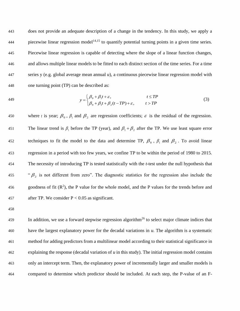
(NINO4); Extreme Eastern Tropical Pacific SST (0 – 10oS, 90oW – 80oW) (NINO12); East Central 434
Tropical Pacific SST (5oN – 5oS) (170oW – 120oW) (NINO34); Oceanic Nino Index (ONI); and 435
Western Hemisphere warm pool (WHWP). Two of the indices describe regional SST in Atlantic 436
oceans—the Tropical Northern Atlantic Index (TNA) and the Tropical Southern Atlantic Index 437
(TSA). The final three indices are the Atlantic Meridional Mode (AMM), the Southern Oscillation 438
Index (SOI), and the 10.7-cm Solar Flux (Solar). 439
440
Statistical analyses. It is apparent that the trend varies in the time series of global and/or regional 441
average mean annual u for different ranges of year (e.g., Fig. 1a). Traditional single linear model 442
does not provide an adequate description of a change in the tendency. In this study, we apply a 443
piecewise linear regression model14,15 to quantify potential turning points in a given time series. 444
Piecewise linear regression is capable of detecting where the slope of a linear function changes, 445
and allows multiple linear models to be fitted to each distinct section of the time series. For a time 446
series y (e.g. global average mean annual u), a continuous piecewise linear regression model with 447
one turning point (TP) can be described as: 448
0 1
0 1 2
,
( ) ,
t t TPy
t t TP t TP
+ + = + + − + (3) 449
where t is year; 0 , 1 and 2 are regression coefficients; is the residual of the regression. 450
The linear trend is 1 before the TP (year), and 1 2 + after the TP. We use least square error 451
techniques to fit the model to the data and determine TP, 0 , 1 and 2 . To avoid linear 452
regression in a period with too few years, we confine TP to be within the period of 1980 to 2015. 453
The necessity of introducing TP is tested statistically with the t-test under the null hypothesis that 454
“ 2 is not different from zero”. The diagnostic statistics for the regression also include the 455
goodness of fit (R2), the P value for the whole model, and the P values for the trends before and 456
after TP. We consider P < 0.05 as significant. 457
458
In addition, we use a forward stepwise regression algorithm26 to select major climate indices that 459
have the largest explanatory power for the decadal variations in u. The algorithm is a systematic 460
method for adding predictors from a multilinear model according to their statistical significance in 461
explaining the response (decadal variation of u in this study). The initial regression model contains 462
only an intercept term. Then, the explanatory power of incrementally larger and smaller models is 463
compared to determine which predictor should be included. At each step, the P-value of an F-464

statistic is calculated to examine models with a potential predictor that is not already in the model. 465
The null hypothesis is that the predictor would have a zero coefficient if included in the model. If 466
there is sufficient evidence at a given significant level to reject the null hypothesis, the predictor is 467
added to the model. Therefore, the earlier the predictor enters in to the model, the larger the 468
explanatory power the predictor has. 469
470
Analyses on the possible causes for the decadal variation in wind speed. Overall, the twenty-471
one climate indices explain 90% of the multi-decadal scale, year-to-year variation in global mean 472
annual u (adjusted R2 = 78%). Regionally, they explain 91%, 75% and 87% of the multi-decadal 473
scale, year-to-year variation in mean annual u for North America (adjusted R2 = 81%), Europe 474
(adjusted R2 = 46%) and Asia (adjusted R2 = 71%), respectively. Globally, the indicators 475
significantly correlated with u include TNA (R = -0.50; P-value < 0.01), PDO (R = 0.46; P < 0.01), 476
WHWP (R = -0.46; P < 0.01), NAO (R = 0.39; P < 0.05), AMM (R = -0.39; P < 0.05), EP/NP (R 477
= 0.37; P < 0.05), TSA (R = -0.38; P < 0.05), Solar (R = 0.35; P < 0.05), SOI (R = -0.32; P < 0.05), 478
and EA (R = 0.31; P < 0.05). All the significant indicators are determined from the SST anomaly 479
over some regions of the tropics, except NAO and EA which are closely relevant to the Arctic 480
oscillation. Among these indicators, TNA is the most significant indicator for u change over North 481
America (R = -0.63; P < 0.01); NAO is the most significant indicator for Europe (R = 0.37; P < 482
0.05); and PDO for Asia (R = 0.50; P < 0.01) (Supplementary Table 2). 483
484
According to the forward stepwise regression analysis, as for global mean annual u, the first six 485
climate indices include in the model are TNA, PDO, AMM, Solar, WHWP, and SCAND 486
(Supplementary Table 3). Regionally, similar to the correlation analysis, TNA has the largest 487

explanatory power for u over North America; NAO has the largest explanatory power for u over 488
Europe; and PDO has the largest explanatory power for u over Asia (Supplementary Table 3). 489
Furthermore, we randomly select 40% of stations for the calculation of global/regional u and repeat 490
the analyses for 300 times to estimate the uncertainty (number in parentheses in Supplementary 491
Table 3 shows how many times climate indices are selected as six major predictors). Last, the six 492
climate indices explain 70 ±5%, 79 ±3%, 48 ±9%, and 51 ±8% of the multi-decadal scale, year-to-493
year variation in mean annual u for the globe, North America, Europe, and Asia, respectively 494
(Supplementary Table 3, Supplementary Fig. 15). 495
496
Calculations for wind power assessments. Due to the nonlinear relationship between wind power 497
(P) and wind speed (u) (Equation (1)), high temporal resolution data are needed for u to produce 498
an accurate estimate of P. Thus, we use the HadISD global sub-daily database from the Met Office 499
Centre19. For each station that has uninterrupted, continuous monthly records during the period 500
1978-2017 (n = 1,542), we use linear interpolation to interpolate a sub-daily time series to an hourly 501
time series. Fig. 4a shows the frequency distributions of global average hourly wind speed in 2010 502
and 2017, and the year 2024, assuming the same increasing rate. 503
504
We then discuss annual wind power production given these wind speed time series (2010, 2017 505
and 2024), considering that production is dependent on the specifications of wind turbines. Here 506
we use General Electric GE 2.5 – 120 (ref. 31) as an example. The parameters for this turbine 507
include the following: rated power, 2,500.0 kW; cut-in wind speed, 3.0 m s-1; cut-out wind speed, 508
25.0 m s-1; diameter, 120 m; swept area, 11,309.7 m2; and hub height: 110/139 m (here we take 509
120 m). The power curve for this turbine is shown in Supplementary Fig. 22. The wind speed time 510

series (2010, 2017 and 2024) at the height of the turbine (i.e. 120 m) are first estimated using the 511
wind profile power law (Equation (2)), and are then converted into the hourly wind power 512
(Supplementary Fig. 19) using the power curve (Supplementary Fig. 22). Owing to the increase 513
frequency of high u, annual wind power production from the turbine increases from 2.4 million 514
kWh in 2010 to 2.8 million kWh in 2017; and to 3.3 million kWh in 2024. As a result, the overall 515
capacity factor increases 1.9% during 2010-2017, and 2.2% during 2018-2024. 516
517
To compare the significance of the increased capacity factor induced by the strengthening u with 518
that due to technology innovation (e.g. improvement of the turbine’s power efficiency), we collect 519
the overall capacity factor for wind generation in the U.S. from the U.S. Energy Information 520
Administration32 (the black line in Fig. 4b). In the U.S., the overall capacity factor is highly 521
correlated with the cube of regional wind speed (u3) (R = 0.86, P < 0.01; Fig. 4b). Even for the 522
detrended time series, the correlation coefficient between capacity factor and u3 is as high as 0.71 523
(P < 0.05), showing that wind speed is a key factor for the year-to-year variation of wind power 524
energy production. It is well known that technology innovation is a key factor that drives the 525
increase of capacity factor for wind generation33. To isolate the u-induced increase in capacity 526
factor from that due to technology innovation, we use the regional mean hourly wind speed in 527
2010, 2017 and 2024 (assuming the same increasing rate) to estimate the increase of capacity factor 528
for a given turbine, thereby controlling for technology innovation. The u-induced increase in 529
capacity factor is +2.5% between 2010 and 2017, and +3.2% between 2017 and 2024. It explains 530
more than 50% of the overall increase of capacity factor for wind generation in the United States. 531
532

We also collect information of the installed turbines from the U.S. Wind Turbine Database (n = 533
57,646; https://eerscmap.usgs.gov/uswtdb) (locations refer to Supplementary Fig. 23). The turbine 534
with the nearest distance to one of the HadISD weather stations (n = 1,542) is at Deaf Smith 535
County, the U.S. (<1 km; wind farm name: Hereford 1; case ID: 3047384; location see the inset 536
plot in Fig. 4c). The turbine was installed in 2014. The turbine is a General Electric GE 1.85 – 87 537
(ref. 34). The parameters for this turbine include: rated power, 1,850.0 kW; cut-in wind speed, 3.0 538
m s-1; rated wind speed, 12.5 m s-1; cut-out wind speed, 25.0 m s-1; diameter, 87.0 m; swept area, 539
5,945.0 m2; hub height: 80 m. We combine these parameters with Equation (1) to estimate the 540
power curve for the turbine (Supplementary Fig. 24). Finally, we integrate the power curve with 541
the hourly wind speed from 1978 to 2017 at the hub height at this station to calculate annual wind 542
power production generated by the General Electric GE 1.85 – 87 turbine (Supplementary Fig. 543
25a; red bars in Fig. 4d). In addition, we calculate annual wind power production at the station 544
generated by the General Electric GE 2.5 – 120 turbine (Supplementary Fig. 25b; green bars in 545
Fig. 4d). We also use the Equation (1) to estimate maximum annual wind power production at the 546
station given diameter of 120 m and hub height of 120 m (the same as the General Electric GE 2.5 547
– 120 turbine), which is constrained by the Betz Limit (f = 16/27 in Equation (1)) (Supplementary 548
Fig. 25c; blue bars in Fig. 4d). The Beltz Limit describes the theoretical maximum ratio of power 549
that can be extracted by a wind turbine to the total power contained in the wind. 550
551
Data availability. The data for quantifying wind speed changes are the Global Surface Summary 552
of the Day database (GSOD, ftp://ftp.ncdc.noaa.gov/pub/data/gsod), and the HadISD (version 553
v2.0.2.2017f) global sub-daily database (https://www.metoffice.gov.uk/hadobs/hadisd/). The time 554
series of climate indices describing monthly atmospheric and oceanic phenomena are obtained 555

from the National Oceanic and Atmospheric Administration 556
(https://www.esrl.noaa.gov/psd/data/climateindices/list/). Simulated wind speed changes in 557
Coupled Model Intercomparison Project Phase 5 (CMIP5) are available in the Program for Climate 558
Model Diagnosis and Intercomparison (https://esgf-node.llnl.gov/projects/cmip5/). Simulated 559
wind speed changes constrained by historical sea surface temperature are provided by the IPSL 560
Dynamic Meteorology Laboratory. Wind records in reanalysis products include the ECMWF 561
ERA-Interim Product (apps.ecmwf.int/datasets/data/interim-full-daily/) and the NCEP/NCAR 562
Global Reanalysis Product (http://rda.ucar.edu/datasets/ds090.0/). The processed wind records and 563
the relevant code are available in Supplementary Data 1 and 2. All datasets are also available on 564
request from Z. Zeng. 565
566
Code availability. The program used to generate all the results is MATLAB (R2014a) and ArcGIS 567
(10.4). Analysis scripts are available by request from Z. Zeng. The code producing wind records 568
are available in Supplementary Data 1 and 2. 569

References. 570
1. Roderick, M. L., Rotstayn, L. D., Farquhar, G. D. & Hobbins, M. T. On the attribution of 571
changing pan evaporation. Geophys. Res. Lett. 34, 1–6 (2007). 572
2. Vautard, R., Cattiaux, J., Yiou, P., Thépaut, J. N. & Ciais, P. Northern Hemisphere atmospheric 573
stilling partly attributed to an increase in surface roughness. Nat. Geosci. 3, 756–761 (2010). 574
3. Mcvicar, T. R., Roderick, M. L., Donohue, R. J. & Van Niel, T. G. Less bluster ahead? 575
ecohydrological implications of global trends of terrestrial near-surface wind speeds. 576
Ecohydrology 5, 381–388 (2012). 577
4. McVicar, T. R. et al. Global review and synthesis of trends in observed terrestrial near-surface 578
wind speeds: Implications for evaporation. J. Hydrol. 416–417, 182–205 (2012). 579
5. Tian, Q., Huang, G., Hu, K., & Niyogi, D. Observed and global climate model based changes 580
in wind power potential over the Northern Hemisphere during 1979–2016. Energy doi: 581
https://doi.org/10.1016/j.energy.2018.11.027iyo (2018). 582
6. Lu, X., McElroy, M. B. & Kiviluoma, J. Global potential for wind-generated electricity. Proc. 583
Natl. Acad. Sci. 106, 10933–10938 (2009). 584
7. Zhu, Z. et al. Greening of the Earth and its drivers. Nat. Clim. Chang. 6, 791–796 (2016). 585
8. Torralba, V., Doblas-Reyes, F. J. & Gonzalez-Reviriego, N. Uncertainty in recent near-surface 586
wind speed trends: a global reanalysis intercomparison. Environ. Res. Lett. 12, 114019 (2017). 587
9. UNFCCC. Adoption of the Paris Agreement (FCCC/CP/2015/L.9/Rev.1., 2015). 588
10. IPCC. Summary for policymakers in Climate change 2014: Mitigation of climate change. 589
Contribution of working group III to the fifth assessment report of the Intergovernmental Panel 590
on Climate Change (O. Edenhofer et al., Eds., Cambridge University Press, Cambridge, UK and 591
New York, USA, 2014). 592

11. U.S. Department of Energy. Projected growth wind industry now until 2050 (Washington, 593
D.C., 2018). 594
12. Nathan, R. & Muller-landau, H. C. Spatial patterns of seed dispersal, their determinants and 595
consequences for recruitment. Trends Ecol. Evol. 15, 278–285 (2000). 596
13. Global Wind Energy Council. Global Wind Energy Outlook 2018 (2018). 597
14. Toms, J. D. & Lesperance, M. L. Piecewise regression: a tool for identifying ecological 598
thresholds. Ecology 84, 2034–2041 (2003). 599
15. Ryan, S. E. & Porth, L. S. A tutorial on the piecewise regression approach applied to bedload 600
transport data (2007). 601
16. Azorin-Molina, C. et al. Homogenization and assessment of observed near-surface wind speed 602
trends over Spain and Portugal, 1961-2011. J. Clim. 27, 3692–3712 (2014). 603
17. Kim, J. C. & Paik, K. Recent recovery of surface wind speed after decadal decrease: a focus 604
on South Korea. Clim. Dyn. 45, 1699–1712 (2015). 605
18. Azorin-Molina, C., Dunn, R. J. H., Mears, C. A., Berrisford, P. & McVicr, T. R. 2018: [Global 606
climate; Atmospheric circulation] Surface winds [in “State of the Climate in 2017”]. Bull. Am. 607
Meteorol. Soc. 99, S41-S43, doi: 10.1175/2018BAMSStateoftheClimate (2018). 608
19. Dunn, R. J. H., Willett, K. M., Morice, C. P. & Parker, D. E. Pairwise homogeneity assessment 609
of HadISD. Clim. Past 10, 1501–1522 (2014). 610
20. Zeng, Z. et al. Global terrestrial stilling: does Earth’s greening play a role? Environ. Res. Lett. 611
Accepted (2018). 612
21. Held, I. M., Ting, M. & Wang, H. Northern winter stationary waves: Theory and modeling. J. 613
Clim. 15, 2125–2144 (2002). 614
22. Hurrell, J. W., Kushnir, Y., Ottersen, G. & Visbeck, M. The North Atlantic Oscillation climatic 615

significance and environmental impact (eds. Hurrell, J. W., Kushnir, Y., Ottersen, G. & Visbeck, 616
M., 2003). 617
23. Kosaka, Y. & Xie, S. P. Recent global-warming hiatus tied to equatorial Pacific surface 618
cooling. Nature 501, 403–407 (2013). 619
24. Wang, C. Z. Atlantic climate variability and its associated atmospheric circulation cells. J. 620
Clim. 15, 1516–1536 (2002). 621
25. Zhang, Y., Xie, S.-P., Kosaka, Y. & Yang, J.-C. Pacific Decadal Oscillation: Tropical Pacific 622
Forcing versus Internal Variability. J. Clim. 31, 8265–8279 (2018). 623
26. Draper, N. R. & Smith, H. Applied Regression Analysis, 3rd Edition (Wiley-Interscience, 624
1998). 625
27. Timmermann, A. et al. El Niño-Southern Oscillation complexity. Nature 559, 535–545 (2018). 626
28. Archer, C. L. Evaluation of global wind power. J. Geophys. Res. 110, D12110 (2005). 627
29. Elliott, D. L., Holladay, C. G., Barchet, W. R., Foote, H. P. & Sandusky, W. F. Wind Energy 628
Resource Atlas of the United States (1986). 629
30. Peterson, E. W. & Hennessey, J. P. On the use of power laws for estimates of wind power 630
potential. Journal of Applied Meteorology 17, 390–394 (1978). 631
31. Wind-turbine-models.com. General Electric GE 2.5 - 120. (2018). at <https://www.en.wind-632
turbine-models.com/turbines/310-general-electric-ge-2.5-120> 633
32. U.S. Energy Information Administration. Capacity Factors for Utility Scale Generators Not 634
Primarily Using Fossil Fuels, January 2013-August 2018. (2018). at 635
<https://www.eia.gov/electricity/monthly/epm_table_grapher.php?t=epmt_6_07_b> 636
33. Dell, J. & Klippenstein, M. Wind Power Could Blow Past Hydro’s Capacity Factor by 2020. 637
(2018). at <https://www.greentechmedia.com/articles/read/wind-power-could-blow-past-hydros-638

capacity-factor-by-2020> 639
34. Wind-turbine-models.com. General Electric GE 1.85 - 87. (2018). at https://www.en.wind-640
turbine-models.com/turbines/745-general-electric-ge-1.85-87 641
35. Steinman, B. A. et al. Atlantic and Pacific multidecadal oscillations and Northern Hemisphere 642
temperatures. Science 347, 988-991(2015). 643
36. Hughes, G. The Performance of Wind Farms in the United Kingdom and Denmark (the 644
Renewable Energy Foundation, 2012). 645
37. Morice, C. P., Kennedy, J. J., Rayner, N. A. & Jones, P. D. Quantifying uncertainties in global 646
and regional temperature change using an ensemble of observational estimates: The HadCRUT4 647
data set. J. Geophys. Res. Atmos. 117, 1–22 (2012). 648
38. Reynolds, R. W., Rayner, N. A., Smith, T. M., Stokes, D. C. & Wang, W. An improved in situ 649
and satellite SST analysis for climate. J. Clim. 15, 1609–1625 (2002). 650
39. WMO Resolution 40 (Cg-XII). Exchanging meteorological data: Guidelines on relationships 651
in commercial meteorological Aativities: WMO policy and practice (WMO, 1996). 652
40. Wallace, J. & Hobbs, P. Atmospheric science: an introductory survey (Academic Press, 2006). 653
41. News, O. S. & Atlantic, N. Surface warming hiatus caused by increased heat uptake across 654
multiple ocean basins. Geophys. Res. Lett. 41, 7868–7874 (2014). 655
42. Makarieva, A. M., Gorshkov, V. G., Sheil, D., Nobre, A. D. & Li, B. L. Where do winds come 656
from? A new theory on how water vapor condensation influences atmospheric pressure and 657
dynamics. Atmos. Chem. Phys. 13, 1039–1056 (2013). 658
43. England, M. H. et al. Recent intensification of wind-driven circulation in the Pacific and the 659
ongoing warming hiatus. Nat. Clim. Chang. 4, 222–227 (2014). 660
44. Chang, P., Ji, L. & Li, H. A decadal climate variation in the tropical Atlantic Ocean from 661

thermodynamic air-sea interactions. Nature 385, 516 (1997). 662
45. European Centre for Medium-Range Weather Forecasts, ERA-Interim Project, 663
https://doi.org/10.5065/D6CR5RD9, Research Data Archive at the National Center for 664
Atmospheric Research, Computational and Information Systems Laboratory, Boulder, Colo. 665
(Updated monthly.) Accessed 10 AUG 2018. 666
46. National Centers for Environmental Prediction/National Weather Service/NOAA/U.S. 667
Department of Commerce, NCEP/NCAR Global Reanalysis Products, 1948-continuing, 668
http://rda.ucar.edu/datasets/ds090.0/, Research Data Archive at the National Center for 669
Atmospheric Research, Computational and Information Systems Laboratory, Boulder, Colo. 670
(Updated monthly.) Accessed 10 AUG 2018. 671
47. Zhu, Z. et al. Global data sets of vegetation leaf area index (LAI)3g and fraction of 672
photosynthetically active radiation (FPAR)3g derived from global inventory modeling and 673
mapping studies (GIMMS) normalized difference vegetation index (NDVI3G) for the period 1981 674
to 2011. Remote Sens. 5, 927–948 (2013). 675
48. Liu, X. et al. High-resolution multi-temporal mapping of global urban land using Landsat 676
images based on the Google Earth Engine Platform. Remote Sens. Environ. 209, 227–239 (2018). 677
Pettitt AN. 1979. A non-parametric approach to the change-point problem. J. R. Stat. Soc. Ser. C: 678
Appl. Stat. 28(2): 126–135. https://doi.org/10.2307/2346729. 679
Copernicus Climate Change Service (C3S) (2017): ERA5: Fifth generation of ECMWF 680
atmospheric reanalyses of the global climate . Copernicus Climate Change Service Climate Data 681
Store (CDS), date of access. https://cds.climate.copernicus.eu/cdsapp#!/home 682
Tsonis, A. A., et al. (2007). "A new dynamical mechanism for major climate shifts." Geophysical 683
Research Letters 34(13): n/a-n/a. 684

Henriksson, S. V. (2018). "Interannual oscillations and sudden shifts in observed and modeled 685
climate." Atmospheric Science Letters 19(10): e850. 686
Wu, J., Zha, J. L., Zhao, D. M., & Yang, Q. D. Changes in terrestrial near-surface wind speed and 687
their possible causes: an overview. Climate Dynamics 51, 2039-2078 (2018). 688
Granger, C.W.J., 1969. "Investigating causal relations by econometric models and cross-spectral 689
methods". Econometrica 37 (3), 424–438. 690
Pryor SC, Barthelmie RJ, Young DT, Takle ES, Arritt RW, Flory D, Gutowski WJ Jr, Nunes A, 691
Roads J. 2009. Wind speed trends over the contiguous USA. Journal of Geophysical Research‐692
Atmospheres 114: D14105, DOI: 10.1029/2008JD011416 693
694
695

Additional information 696
Supplementary information is available in the online version of the paper. Reprints and 697
permissions information is available online at www.nature.com/reprints. 698
Correspondence and requests for materials should be addressed to Z. Zeng. 699
700
Acknowledgements 701
This study was supported by Lamsam-Thailand Sustain Development (B0891). J. Liu was 702
supported by the National Natural Science Foundation of China (41625001). We thank Della 703
Research Computing in Princeton University for providing computing resources. We thank the 704
USA? National Climatic Data Center and the UK Met Office Centre for providing surface wind 705
speed measurements, and thank the Program for Climate Model Diagnosis and Intercomparison 706
and the IPSL Dynamic Meteorology Laboratory for providing surface wind speed simulations. 707
708
Author contributions 709
Z. Zeng and E. Wood designed the research. Z. Zeng and L. Yang performed analysis; Z. Zeng, A. 710
Ziegler, T. Searchinger wrote the draft; and all the authors contributed to the interpretation of the 711
results and the writing of the paper. 712
713
Competing financial interests 714
The authors declare no competing financial interests. 715
716
717

Figure Legends. 718
Figure 1. Turning point for mean global surface wind speed (u). (a) Global mean annual u 719
during 1978-2017 (black dot and line). The piecewise linear regression model indicates a 720
statistically significant turning point in 2010. The red line is the piecewise linear fit (R2 = 90%, P 721
< 0.001). The dashed line indicates the turning point. The trends before and after the turning point 722
are shown in the inset. Each grey line (n = 300) is a piecewise linear fit for a randomly selected 723
subset (40%) of the global stations. (b) Frequency distribution of the estimated turning points 724
derived from the 300 resampling results. (c) Frequency distribution of the trends in mean annual 725
u before and after the turning point from the 300 resampling results. The result is grounded on the 726
weather stations in the GSOD database. 727
Figure 2. Factors driving the decadal variations in u. Observed (red) and reconstructed (black) 728
detrended mean annual u over the following: (a) the globe, (b) North America, (c) Europe, and (d) 729
Asia. For the globe and each of the three continents, we select six largest explanatory climate 730
indices for the decadal variations of u with a stepwise forwarding regression model. The selected 731
climate indices are then used to reconstruct decadal variations of u via a multiple regression. 732
Uncertainties are the inter-quartile range of the results based on a randomly selected 40% subset 733
of the station pools (repeated 300 times). Inset plots indicate the locations of the stations. The 734
models are trained only using the detrended time series before the turning points. The dashed line 735
indicates the turning point (2010 for the globe, 2012 for North America, 2003 for Europe, and 736
2001 for Asia). Inset black numbers are coefficients of determination between observed and 737

reconstructed u before the turning points. Inset red numbers are correlation coefficient and its 738
significance between observed and reconstructed u after the turning points. 739
Figure 3. Mechanisms for the decadal variation in u. Normalized mean annual surface 740
temperature for the years with negative (a) and positive (b) anomalies of detrended wind. 741
Characteristic regions for Pacific Decadal Oscillation (PDO), North Atlantic Oscillation (NAO) 742
and Tropical Northern Atlantic Index (TNA) are outlined by green, red, and blue boxes, 743
respectively. Surface temperature over land is obtained from Climate Research Unit TEM4 with a 744
spatial resolution of 5° by 5° (ref. 37), and that over ocean is from NOAA Optimum Interpolation 745
(OI) Sea Surface Temperature V2, with a spatial resolution of 1° by 1° (ref. 38). Spatial patterns 746
of the correlation between the regional (5o × 5o) mean annual u and the following: (c) TNA; (d) 747
NAO; and (e) PDO for 1978-2017. Dotting represents significant at P < 0.05 level. Decadal 748
variations are shown in panels (f) for TNA and regional u in North America; (g) for NAO and 749
regional u in Europe; and (h) for PDO and regional u in Asia. The thin lines are annual values; and 750
the thick lines are 9-year-window moving averages. The black lines are wind speed; and each of 751
the colored lines are TNA, NAO, and PDO, respectively. 752
Figure 4. Implications of the recent reversal in global terrestrial stilling for wind energy 753
industry. (a) Frequency distribution of global average hourly u in 2010 and 2017, and the year 754
2024 assuming the same increasing rate. (b) Time series of the overall capacity factor for wind 755
generation in the U.S. (black line) and the three-order of the regional-average u (u3; blue line) from 756
2008 to 2017. The inset scatter plot shows the significant relationship between the overall capacity 757
factor and the regional u3 (R = 0.86, P < 0.01). The inset black numbers show the trend in the 758
overall capacity factor for wind generation, and the inset red numbers show the u-induced increase 759
of capacity factor in the USA. (c) Mean annual u observed at a weather station near an installed 760

turbine at Deaf Smith County, USA. (<1 km). The inset plot shows the location. The turbine was 761
installed in 2014. The background colors separate different periods: P0, the 1980s level when u is 762
relative strong (1978-1995); P1, the evaluation years before the installation of the turbine (2009-763
2013); P2, the operation years when the turbine is generating power (2014-2017). (d) Mean annual 764
wind power production at Deaf Smith County, the U.S. from different wind turbines during 765
different periods (red: General Electric GE 1.85 – 87; green: General Electric GE 2.5 – 120 turbine; 766
blue: the theoretical maximum ratio of power that can be extracted by a wind turbine given 767
diameter of 120 m and hub height of 120 m). Error bars show the interannual variability within the 768
periods. 769
770
771

Figure 1. Turning point for mean global surface wind speed (u). (a) Global mean annual u 772
during 1978-2017 (black dot and line). The piecewise linear regression model indicates a 773
statistically significant turning point in 2010. The red line is the piecewise linear fit (R2 = 90%, P 774
< 0.001). The dashed line indicates the turning point. The trends before and after the turning point 775
are shown in the inset. Each grey line (n = 300) is a piecewise linear fit for a randomly selected 776
subset (40%) of the global stations. (b) Frequency distribution of the estimated turning points 777
derived from the 300 resampling results. (c) Frequency distribution of the trends in mean annual 778
u before and after the turning point from the 300 resampling results. The result is based on the 779
weather stations in the GSOD database. 780
781
782

Figure 2. Factors driving the decadal variations in u. Observed (red) and reconstructed (black) 783
detrended mean annual u over the following: (a) the globe, (b) North America, (c) Europe, and (d) 784
Asia. For the globe and each of the three continents, we select six largest explanatory climate 785
indices for the decadal variations of u with a stepwise forwarding regression model. The selected 786
climate indices are then used to reconstruct decadal variations of u via a multiple regression. 787
Uncertainties are the inter-quartile range of the results based on a randomly selected 40% subset 788
of the station pools (repeated 300 times). Inset plots indicate the locations of the stations. The 789
models are trained only using the detrended time series before the turning points. The dashed line 790
indicates the turning point (2010 for the globe, 2012 for North America, 2003 for Europe, and 791
2001 for Asia). Inset black numbers are coefficients of determination between observed and 792

reconstructed u before the turning points. Inset red numbers are correlation coefficient and its 793
significance between observed and reconstructed u after the turning points. 794
795
796

Figure 3. Mechanisms for the decadal variation in u. Normalized mean annual surface 797
temperature for the years with negative (a) and positive (b) anomalies of detrended wind. 798
Characteristic regions for Pacific Decadal Oscillation (PDO), North Atlantic Oscillation (NAO) 799
and Tropical Northern Atlantic Index (TNA) are outlined by green, red, and blue boxes, 800
respectively. Surface temperature over land is obtained from Climate Research Unit TEM4 with a 801

spatial resolution of 5° by 5° (ref. 37), and that over ocean is from NOAA Optimum Interpolation 802
(OI) Sea Surface Temperature V2, with a spatial resolution of 1° by 1° (ref. 38). Spatial patterns 803
of the correlation between the regional (5o × 5o) mean annual u and the following: (c) TNA; (d) 804
NAO; and (e) PDO for 1978-2017. Dotting represents significant at P < 0.05 level. Decadal 805
variations are shown in panels (f) for TNA and regional u in North America; (g) for NAO and 806
regional u in Europe; and (h) for PDO and regional u in Asia. The thin lines are annual values; and 807
the thick lines are 9-year-window moving averages. The black lines are wind speed; and each of 808
the colored lines are TNA, NAO, and PDO, respectively. 809
810
811

Figure 4. Implications of the recent reversal in global terrestrial stilling for wind energy 812
industry. (a) Frequency distribution of global average hourly u in 2010 and 2017, and the year 813
2024 assuming the same increasing rate. (b) Time series of the overall capacity factor for wind 814
generation in the U.S. (black line) and the three-order of the regional-average u (u3; blue line) from 815
2008 to 2017. The inset scatter plot shows the significant relationship between the overall capacity 816
factor and the regional u3 (R = 0.86, P < 0.01). The inset black numbers show the trend in the 817
overall capacity factor for wind generation, and the inset red numbers show the u-induced increase 818
of capacity factor in the United States. (c) Mean annual u observed at a weather station near an 819
installed turbine at Deaf Smith County, the U.S. (<1 km). The inset plot shows the location. The 820
turbine was installed in 2014. The background colors separate different periods: P0, the 1980s 821
level when u is relative strong (1978-1995); P1, the evaluation years before the installation of the 822
turbine (2009-2013); P2, the operation years when the turbine is generating power (2014-2017). 823
(d) Mean annual wind power production at Deaf Smith County, the U.S. from different wind 824

turbines during different periods (red: General Electric GE 1.85 – 87; green: General Electric GE 825
2.5 – 120 turbine; blue: the theoretical maximum ratio of power that can be extracted by a wind 826
turbine given diameter of 120 m and hub height of 120 m). Error bars show the interannual 827
variability within the periods. 828
829