Wing-, cube- and aeroelastic simulations in

Unicorn

Kenny HedlundMaster Thesis

Royal Institute of Technology, 100 44, Stockholm, Sweden

December 20, 2010

Abstract

The new FEM computational fluid dynamics software, Unicorn, has been used for aerodynamicforce estimation on a cube and a NACA0012 wing spanning a wind tunnel. It has also been usedfor an elastic plate, showing that aeroelastic problems may be solved in a near future. This hasbeen done, modeling the boundary layer with slip condition. For the wing, the fluid has alsobeen modelled as completely inviscid.The cube drag computation has indicated convergence towards the experimental drag coefficientof 1.05 within a few percent. The wing simulations on the other hand have proven to give rise tomore problems. Here, a set of different boundary conditions, meshes and normal computationmethods have been evaluated. Most of the results have shown fairly good lift computations(within a few percent of the experimental values), but all has shown too large drag estimations.They do however tend to decrease when the mesh is refined, with the adaptive mesh refinementfunctionality. The results have also proven to replicate experiments well in a qualitative manner,like oil flow visualisation and circulation patterns.I has been concluded that edge conditions should be avoided, in order to get pure slip conditioneverywhere and that superparametric elements should be used in order to avoid artificial frictionfrom velocity projection at the nodes. Further concluions are that it is crucial to move addednodes, from adaptive mesh refinement, to the exact geometry and that computations should bemade for large aircraft or wings with wing tips, since the too large drag might be vanishinglysmall in comparison to larger scale drags like wing tip vortices.

Nomenclature

b = Wing spanC = Constantc = Wing chordCD = Drag coefficientCL = Lift coefficientD(·) = Derivation operator w.r.t (·)F = Displacement rate vector [m/s]f = Volume force vector [N]G = Structural shear modulus [Pa]h = Mesh size [m]I = Time domain [0,T]I = The identity matrixk = Time step [s]K = Finite element in meshM = Magnitude of interestn = Normal vectorp, p, P, q = Pressures [Pa]Pp = Particle positionqF ,vF = Finite element functionsQ = Space-time domainR = Residual vectort = Tangential vectort = Time [s]T = Final timeu, U, w , v = Velocity vectors [m/s]X,x = Particle original positionα = Angle of attack (a.o.a) [deg]µ,E = Isotropic Young’s modulus [Pa]ν = Kinematic viscosity [m2/s]∂Ω = Space boundaryΩ = Space domainϕ = Dual velocityψ = Dual magnitude of interestρ = Density [kg/m3]ρs = Structure density [kg/m3]τn = Finite element meshθ = Dual pressure

1

1 Introduction

It is not hard to realise that it is necessary to ensure that the wings should not be subject tostructural failure, and that this requires some means of estimating the structural displacementresulting from air loads. One way of doing this is by estimating the aerodynamics with unsteadypotential flow theory and linearizing the equations of motion around some given condition. Thisenables a stability analysis of both the dynamic and static behaviour of the wing and also givesthe possibility to estimate static deformations.

The static stability analysis is typically used to predict divergence and reversal. Divergencehappens when the aerodynamic forces are reducing the effective stiffness of the wings to zero orfurther in some direction, and thus, potentially leading to very large deformations. This may ofcourse have catastrophic consequences. Reversal is when the effectiveness of a control surface isreduced because of the moment that twists the lifting surface and thereby changes the angle ofattack in such a way that it counteracts the lift produced by the control surface itself.

The dynamic stability is governing what is known as flutter. This is when a perturbationof the deformation results in an oscillating motion which is undamped, or negatively damped.Even though this may be described by a linear system of equations, the stability analysis is nottrivial to resolve. The reason for that, is that it results in a nonlinear eigenvalue problem, andtherefore requires an iterative solution process. Nevertheless, this method is relatively fast, andtherefore a very powerful tool. However, this speed does not come completely without flaws;since it is based on potential flow theory, the accuracy may be quite low, and completely unableto predict the nonlinear regime of the flow. Thus it may be of interest to investigate linearinstabilities further, using more accurate CFD methods, so that more accurate results may beobtained. Therefore this report will investigate the possibility to solve the aerodynamics and thestructural mechanics simultaneously for an aeroelastic problem.

The software that will be used in this study is capable of solving fluid-structure interactionas one problem, which makes it ideal for space-time simulations of aeroelastic problems. It iscalled Unicorn, and forms a part of the FEniCS project [1]. This is however based on a ratherunconventional approach to obtaining accurate CFD solutions, explained insection 2.1, which iswhy it will need to be tried for some basic purely aerodynamic problems for justification of theuse of this software.

2

2 Theory

2.1 Aerodynamic Modeling

In today’s fluid dynamics, a no slip BC (Boundary Condition), along with the incompressibleNavier-Stokes (ICNS) system of equations, (1), is needed for accurate estimations of subsonicfluid flows. (No slip means that the air has zero relative velocity compared to the boundary onthe boundary, while slip allows tangential velocities.)

u + (u · ∇)u− ν∆u +∇pρ

= f , in Q

∇ · u = 0, in Q (1)

u = 0, on ∂Ω× I

Figure 1: Depiction of the domain..

Q is the considered domain for the entire considered time and I is the time domain [0,T].Therefore, viscous effects have a large impact on the flow close to the surface, even in almost

inviscid fluids, forming a viscous boundary layer (BL). This is of major importance since thisprovides an explanation to lift and drag. However, a new explanation has been presented byClaes Johnson and Johan Hoffman in [6], where they claim that this may be obtained accuratelywithout boundary layers.

This might be a major break through in fluid dynamics, since it would allow for the flowto be computed without resolving the small boundary layers, present in high Reynolds numberproblems for large structures, potentially allowing for a great reduction in mesh points.

2.1.1 Impact of Boundary Layers

If the viscosity is zero and a slip BC is applied, equation 1 turns into the incompressible Eulerequations, (2).

u + (u · ∇)u +∇pρ

= f , in Q

∇ · u = 0, in Q (2)

u · n = 0, on ∂Ω× I

3

These equations can be solved analytically for e.g. the flow around a wing using potentialtheory. When this is done, one obtains a clearly unphysical result, namely that the forces fromthe flow on the wing is zero. BL theory explains this by stating that the boundary layer generatescirculation, causing the flow to be faster on the upper side than the lower side. This also createsan up draught upstream of the wing and a down draught downstream. These phenomena result inforces on the body, which should be expected. BL theory may also be used to explain separationand the difference between turbulent and laminar separation.

Johnson and Hoffman, however, claim that the potential solution is unstable to perturbationsand that it is therefore it cannot be observed in reality. This may be shown by equations (2)-(5).Consider two solutions to equation (2), (w, p) and (u, p).

w + (w · ∇)w +∇pρ

= f , in Q

∇ ·w = 0, in Q (3)

w · n = 0, on ∂Ω× I

By subtracting (2)-(3), one obtains a linearized Euler equation (4).

v + (u · ∇)v + (v · ∇)u +∇qρ

= 0, in Q

∇ · v = 0, in Q (4)

v · n = 0, on ∂Ω× I,

where the quadratic perturbation terms have been omitted, with

v = u−w

q = p− p

and since

Σ(diag(A)) = Σ(eig(A)), for any matrix A

⇒ Σ(eig(∇u)) = 0 (5)

This means that ∇u has positive eigenvalues, unless the real parts of the diagonal are allzero. Therefore, exponential growth of perturbations is expected.

2.1.2 FEM

Unicorn uses a Finite Element Method named the G2 (Galerkin 2) - method, by Johnson andHoffman [6]. This solves (1), but with slip BC instead of no slip.

The time stepping, U, can be viewed as Crank-Nicholson for solutions that are piecewiselinear in space and time. This is done by iterating (for ν = 0),

Ui+1n+1 =Un + k(0.5f(Ui

n+1) + 0.5f(Uin)),

f(U)in+1 =−Uin+1 · ∇Ui

n+1 −∇pin+1,

4

where i, indicates the iteration number and Un = U(tn).The choice of k is made so that it satisfies

k ≤ hmin

| U |. (6)

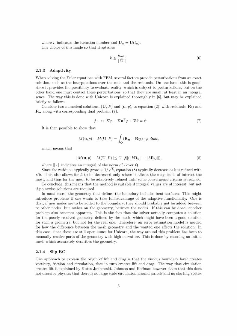
2.1.3 Adaptivity

When solving the Euler equations with FEM, several factors provide perturbations from an exactsolution, such as the interpolations over the cells and the residuals. On one hand this is good,since it provides the possibility to evaluate reality, which is subject to perturbations, but on theother hand one must control these perturbations, so that they are small, at least in an integralsence. The way this is done with Unicorn is explained thoroughly in [6], but may be explainedbriefly as follows.

Consider two numerical solutions, (U, P ) and (u, p), to equation (2), with residuals, RU andRu along with corresponding dual problem (7).

−ϕ− u · ∇ϕ+∇uTϕ+∇θ = ψ (7)

It is then possible to show that

M(u, p)−M(U, P ) =

∫Q

(Ru −RU) · ϕ dxdt,

which means that

|M(u, p)−M(U, P ) |≤ C‖ϕ‖(‖hRu‖+ ‖hRU‖), (8)

where ‖ · ‖ indicates an integral of the norm of · over Q.Since the residuals typically grow as 1/

√h, equation (8) typically decrease as h is refined with√

h. This also allows for h to be decreased only where it affects the magnitude of interest themost, and thus for the mesh to be adaptively refined until some convergence criteria is reached.

To conclude, this means that the method is suitable if integral values are of interest, but notif pointwise solutions are required.

In most cases, the geometry that defines the boundary includes bent surfaces. This mightintroduce problems if one wants to take full advantage of the adaptive functionality. One isthat, if new nodes are to be added to the boundary, they should probably not be added betweento other nodes, but rather on the geometry, between the nodes. If this can be done, anotherproblem also becomes apparent. This is the fact that the solver actually computes a solutionfor the poorly resolved geometry, defined by the mesh, which might have been a good solutionfor such a geometry, but not for the real one. Therefore, an error estimation model is neededfor how the difference between the mesh geometry and the wanted one affects the solution. Inthis case, since these are still open issues for Unicorn, the way around this problem has been tomanually resolve parts of the geometry with high curvature. This is done by choosing an initialmesh which accurately describes the geometry.

2.1.4 Slip BC

One approach to explain the origin of lift and drag is that the viscous boundary layer createsvorticity, friction and circulation, that in turn creates lift and drag. The way that circulationcreates lift is explained by Kutta-Joukowski. Johnson and Hoffman however claim that this doesnot describe physics; that there is no large scale circulation around airfoils and no starting vortex

5

[7]. Instead, they have presented a new explanation [7] that supposedly explains both lift anddrag, see figure 2.

Figure 2: Johnson/Hoffman’s alternative to Kutta-Joukowski [7].

When two flow streams are converging on the downstream side of 3D objects, a transverseflow is induced, that in turn induces streamwise vorticity. This allows for low pressure vorticesto pull down the flow towards the surface and thus creating lift and drag on airfoils.

What might introduce some problems here however, is the fact that the slip boundary condi-tion requires the surface normals. These may be defined as giving the node normals the mean ofthe surrounding facets’ normals, weighted by their areas. This might, however introduce errors inthe normals in a way that they do not exactly correspond to the normals of the actual geometryin the corresponding points. This might be solved by extracting the the true normal distributionfrom the geometry, and importing it in the solver, in order to get the true values in the nodes.That functionality is under development for Unicorn, but not yet incorporated. Therefore alsothis problem requires curved surfaces to be accurately defined already in the initial mesh.

Furthermore, when a geometry has edges or corners, the normals are not defined exactly onthe edge. This might be solved by using the mean value of the surrounding facets as describedabove. That might however induce a flow through the facets. To solve this, Unicorn has amaximum angle between the face normals, above which the node is defined as an edge node orcorner node, depending on the number of directions of nearby facet inclinations. This is doneby enforcing slip condition for both surrounding normals (edge) or no slip (corner). The defaultmaximum facet inclination angle in Unicorn is set to π

6 . However, since having an edge at thetrailing edge at the trailing edge will enforce a stagnation point at the trailing edge and a ”bubbleof slow air” of the size of the trailing edge cells, investigation is required as to whether the edgecondition should be present there. It is also to be investigated whether or not the edge criteriumis needed in the boundary between e.g. wings and wind tunnel walls.

2.1.5 Turbulence

As stated earlier, [6], argues that the potential solution is unstable to perturbations. This isshown in the analysis of the linearized Euler equations, but may also be shown by the vorticityequation, (9), explaining the large amount of vorticity, present in turbulent flows.

ω + (u · ∇)ω − (ω · ∇)u = 0 (9)

If one then focuses on the potential solution in the circular cylinder case, φ(x1, x2) = (r +1r )cos(β), being the real part of the analytic function w = z + 1

z with z = x1 + ix2, one gets

6

w(z) = z − 1 + 1 +1

z − 1 + 1≈ 2 + (z − 1)2

⇒ φ(x1, x2) ≈ 1 + (x1 − 1)2 − x22 (10)

⇒ u(x) = (2(x1 − 1),−2x2, 0)

Figure 3: Cylinder case definition.

Thus, (9) takes the form

ω1 + (u · ∇)ω1 =2ω1

ω2 + (u · ∇)ω2 =− 2ω2 (11)

ω3 + (u · ∇)ω3 =0,

close to the point z = 1 (the downstream stagnation point), which means that ω1 growsexponentially and thus that strong vorticity will be generated close to the rear stagnation point.

Equation (8) shows that the residuals may be pointwise large for small h, without having largeimpact on the mean value output of the magnitude of interest. This would be critical in caseyou get blow up when solving a problem, because even if the residual grows as the spacial stepsize is decreased, the reduction of h might counteract that growth. This is exactly what [6] claimhappens when the NS are solved with the G2 method, see equations (12).

R(U) ∼ h−1/2

|M(u, p)−M(U, P ) |≤ C‖ϕ‖(‖hRu‖+ ‖hRu‖) ∼ C‖ϕh1/2, (12)

This means that you would expect a turbulent solution to blow up and be wrong everywhere,but show a mean value convergence as the mesh is refined.

7

An example of this is shown in the following scalar linear constant coefficient stationary modelproblem.

u,1 + u− νδu = f, in Ω, u = 0, on Γ, (13)

where ν is small and Ω = (0, 1)2 with boundary Γ, u,1 = ∂u∂x1

and f is a given function. Thenlet U be a continuous piecewise linear G2 solution defined by

(U,1 + U, v + hv,1 = (f, v + hv, 1)) (14)

where (·, ·) is the L2(Ω)-norm, since ν << h and the stabilizing term, h(v,1 + v), has beensimplified to hv,1. With the L2(Ω)-norm ‖ · ‖, v = U , ‖f‖ = 1 the following energy estimate,

‖U‖2 + ‖√hU2

,1 ≤ (1 + h)‖f‖2 ≈ 1 (15)

shows that the stabilizing term ‖√hU,1‖2 will not be small in case the exact solution has

layers, because U,1 ∼ h−1 in an outflow layer of width ∼ h, and U,1 ∼ h−1/2 in characteristiclayers of width h1/2. Thus

R(U) ≈U,1 + U − f⇒ choose v =U ⇒ (16)

⇒ −(R(U), U) ≈‖√hU,1‖2 >> 0,

which shows that R(U) cannot be small everywhere, but with R(U) ∼ h−1 in the outflowlayers and R(U) ∼ 1 in the characteristic layers (parallel to boundary), then

|M(u)−M(U) |∼ h3/2, (17)

if M(u) = (u, ψ) and ψ vanishes in the layers. Then again, the error in output of interestmay be small even though the residuals are pointwise large (”output of interest” is a quantity ofwhich one may be interested, eg. a space intergral of the pressure on one of the boundaries). [6]

2.2 Structural Modeling

The constitutive modeling is derived by first expressing the displacement rate as function oforiginal particle position, time and velocity. This is described in equations (18). The displacementrate in one element contributes its velocity along with the neighbours’ displacement rates, thattranslates and rotates the element like a rigid body.

DtF(t,Pp(t,X)) = DtDXPp(t,X)

= DXu(t,Pp(t,X))

= Dpu(t,Pp(t,X))DXPp(t,X)

= ∇u(t,Pp(t,X))F (t,Pp(t,X))

⇔ DtF = ∇uF

⇒ DtF−1 = −F−1∇u (18)

Using the relation

8

B = FFT ,

equation (18) may be modified to exclude the displacement rate. This may be achieved byusing the Neo-Hookean constitutional equation (19).

σ = µ(B− I)− pI (19)

If we differentiate the component

σD = µ(B− I), (20)

with respect to time, using the relation

DtB = ∇uB + B∇uT , (21)

and equation (20), we obtain equation (22).

DtσD = µ2ε(u) +∇uσD + σD∇uT (22)

Thus, we may solve a rate problem, which is equivalent to the non rate model (20). Sincethe aerodynamic problem uses a rate model, this allows for the whole domain to be solvedsimultaneously given only the model parameters and an indicator that defines which cells arestructure and which ones are fluid.

This, does however require some approximations:

• Only choosing the σD part of the problem approximates the solid as incompressible.

• Using a scalar µ instead of a stiffness matrix, E, only allows for isotropic material models(which is the case for the code at the moment).

2.3 ALE

In aerodynamic problems, an Eulerian representation is most convenient, while in structuralproblems, a Lagrangian representation is easier. Therefore, an ideal way of solving a fluid-structure interaction problem would be to use Eulerian coordinates for the fluid and Lagrangiancoordinates for the structure. This may be done by moving the structural part of the mesh insidethe fluid part and adding the mesh velocity, w to the fluid equations of motion, see equation(23).

˙(u) + ((u−w) · ∇)(u) +∇pρ

= 0 (23)

This however, requires that the mesh must be smoothed in some way, in order to avoid bad orinverted elements. One way of doing this is by elastic mesh smoothing, which is briefly describedby equations (24).

σ = E(I− (FFT )−1)

DtF−1 = −F−1∇w, (24)

with the initial condition on F that it corresponds to the deformation gradient with regardto a scaled equilateral reference cell.

9

3 Method

3.1 Mesh generation

The mesh generator chosen was Salome [2], because it is open source and because it is possibleto load coordinate files for creating geometries. Another advantage with Salome is the scriptfunctionality, allowing the user to change parameters without having to redraw/remesh manually.It also allows exchanging scripts of a few kB instead of meshes tens or hundreds of MB, whenmore than one person is involved in the process. An example of a script for creating a uniformtetrahedral mesh of a cube in a tunnel is presented in figure 4.

import smeshimport geompyimport salomeimport StdMeshersimport NETGENPluginimport mathgg = salome.ImportComponentGUI("GEOM")

box1 = geompy.MakeBox(-0.1, -0.1, -0.1, 0.1, 0.1, 0.1)box2 = geompy.MakeBox(-2.0, -0.5, -0.5, 5.0, 0.5, 0.5)cut = geompy.MakeCut(box2, box1)geompy.addToStudy( cut, "cut" )

print 'Geometry computed'

Mesh_1 = smesh.Mesh(cut)Regular_1D = Mesh_1.Segment()Max_Size_1 = Regular_1D.MaxSize(0.2)MEFISTO_2D = Mesh_1.Triangle(algo=smesh.NETGEN_2D)Tetrahedron_Netgen = Mesh_1.Tetrahedron(algo=smesh.NETGEN)isDone = Mesh_1.Compute()

if not isDone: print 'Mesh computation failed'print "Done"

Figure 4: Simple cube mesh script for Salome.

However, since the dolfinXML mesh format is not available in Salome, a file format conversionprogram has been created. This simply reads the relevant data in a unv-file (available in Salome)to save in dolfinXML, see figure 5.

Corresponding dolfinXML file would then be the one described by figure 6.The cube case was solved using a uniform tetrahedral mesh with 3750 nodes as initial mesh.

This mesh was provided by Murtazo Nazarov.The wing section was generated by interpolating the coordinates shown in table 11 in the

appendix using bezierinterpolation, after scaling, rotating and translating the coordinates aroundthe geometric center of the wing section to fit the corresponding test case, see equation (25).

10

-1 2411 Node number 1 0 0 11 9.9697909977647450E-02 -7.8189990464832444E-03 2.5000000000000000E-01

.

.

. 23004 0 0 11 9.5590578885975636E-02 -6.7347100893712887E-03 -2.4953780229824737E-01 -1 -1 Node coordinates 2412 1 11 2 1 7 2 0 0 0 1D elements 17 4

.Element number .

. 1311 41 2 1 7 3 17 4 2 2D elements

.

.

. 146759 111 2 1 7 4 21576 21575 9453 9424 3D elements -1 Nodes in element

Figure 5: UNV-mesh example from Salome. Necessary mesh information for dolfinXML filesencircled (only 3D elements are needed).

xtransformed = c ∗(

(xtable −1

2) ∗ cos(α) + ytable ∗ sin(α) +

1

2

)ytransformed = c ∗

(−(xtable −

1

2) ∗ sin(α) + ytable ∗ cos(α)

)(25)

ztransformed = z

For the wing meshes, the attempts to use the NETGEN 1D-2D-3D generator with meshoptimization were unsuccessful, which is why manual choices of mesh sizes for different domainswere needed. The two different 1-D mesh size configurations that have been used in the projectare presented in table 1.

Four subdomains were used in order to enable different cell sizes at different locations in themesh. These are presented in figure 7.

To create the leading edge subdomains, the same procedure was performed for the same wing,scaled and translated to form a surrounding layer for an amount of points corresponding to thelength of the domain. Then all faces were extruded with the span of the wing and put inside atunnel with some appropriate cut/merge operations.

The flutter plate mesh was created using the NETGEN 1D-2D-3D algorithm. In order toavoid having to have no slip boundary conditions at the junction between the flutter plate and

11

<?xml version="1.0" encoding="UTF-8"?>

<dolfin xmlns:dolfin="http://www.fenics.org/dolfin/"><mesh celltype="tetrahedron" dim="3"><vertices size="23004">

<vertex index="0" x="0.0996979" y="-0.007819" z="0.25" />...

<vertex index="23003" x="0.0955906" y="-0.00673471" z="-0.249538" /></vertices><cells size="132011">

.

.

.<tetrahedron index="132010" v0="21575" v1="21574" v2="9452" v3="9423" />

</cells></mesh></dolfin>

Figure 6: DolfinXML file corresponding to the UNV file in figure 5.

Parameter 20k node mesh value 100k node mesh valueDomain 1 maximum 1D length 0.4 [m] 0.2 [m]Domain 2 maximum 1D length 0.1 [m] 0.05 [m]Domain 3 maximum 1D length 0.02 [m] 0.01[m]Domain 4 maximum 1D length 0.01 [m] 0.005[m]1D mesh generation algorithm Regular 1D Regular 1D2D mesh generation algorithm Mephisto 2D triangle Mephisto 2D triangle3D mesh generation algorithm Netgen 3D tetrahedron Netgen 3D tetrahedron

Table 1: Mesh specifications for wing case sub domains. Geometry and mesh generated withSalome [2].

the wind tunnel wall, the wind tunnel was divided into two sub domains, where the structuralone formed the plate and the wall, see figure 8 and table 2.

3.2 Manual wing surface normal computation

In order to manually compute the surface normals for the NACA0012 profile, one needs the wingsection equation (26) [5].

y

c= ±0.6[0.2969

√x/c− 0.126x/c− 0.3516(x/c)2 + 0.2843(x/c)3 − 0.1015(x/c)4] (26)

However, in order for equation (26) to be valid for a given node, that node’s coordinates haveto be rotated back from the present angle of attack to 0 degrees (see section sec:mesh). Then,in order to get the node normal in the rotated coordinate system, one may simply derivate thewing section equation and choose a vector, perpendicular to the derivative vector, see equations(27) and (28).

12

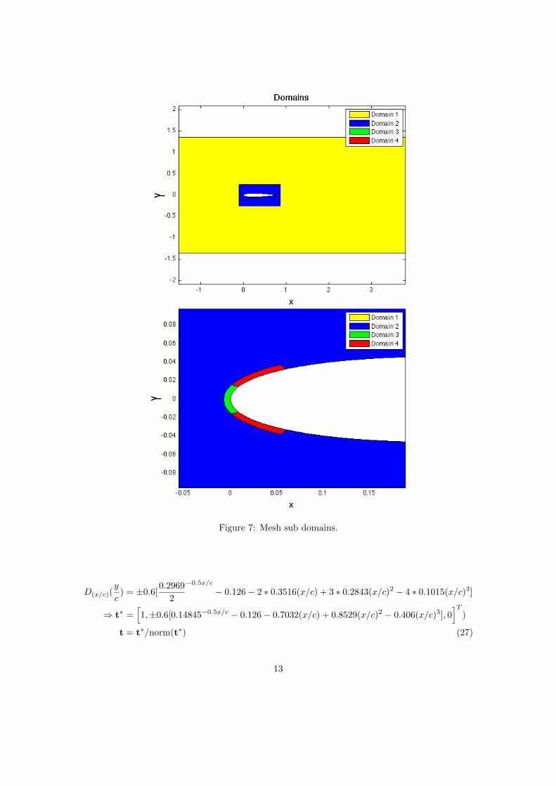
Figure 7: Mesh sub domains.

D(x/c)(y

c) = ±0.6[

0.2969

2

−0.5x/c

− 0.126− 2 ∗ 0.3516(x/c) + 3 ∗ 0.2843(x/c)2 − 4 ∗ 0.1015(x/c)3]

⇒ t∗ =[1,±0.6[0.14845−0.5x/c − 0.126− 0.7032(x/c) + 0.8529(x/c)2 − 0.406(x/c)3], 0

]T)

t = t∗/norm(t∗) (27)

13

Mesh generation algorithm Netgen 1D-2D-3D tetrahedronTotal number of elements ca 130 000

Table 2: Flutter plate mesh specifications. Geometry and mesh generated with Salome [2].

Figure 8: Structural domain in flutter plate mesh.

Since the z-component is zero, one may then simply switch places of the x- and y-componentsand times on of them with -1.

⇒ n =[±0.6[0.14845−0.5x/c − 0.126− 0.7032(x/c) + 0.8529(x/c)2 − 0.406(x/c)3],−1, 0

]T/norm(t∗))

(28)

14

4 Case Setups

4.1 Cube

The cube test case is made to try out the capabilities of the flow part of the solver to catchflow scenarios with large amounts of separation. Therefore, a cube aligned with the xyz-axesand corners in (0.6,0.4,0.4) and (0.8,0.6,0.6) is placed in a square tunnel, also aligned with thecoordinate axes, with corners in (0,0,0) and (3,1,1). The Initial mesh is composed of 18 000uniformly sized tetrahedrons. The parameters used for simulating the flow solution are shownin table 3.

ν [2 · 10−3, 2 · 10−5, 2 · 10−7] [m2/s]ρ 1 [kg/m3]

Number of adaptive iterations 10Percentage of cells to be refined/adaptive iteration 10

Time span [0,10] [s]Inflow velocity (1,0,0) [m/s]

Outflow p = 0 [Pa]Tunnel wall & cube Slip

Table 3: Parameters used for cube flow computation.

4.2 NACA0012 Airfoil

In order to validate also lift and drag, and their origins, the flow around a NACA0012 will alsobe computed.

The geometric and aerodynamic characteristics are defined in table 4 and the BCs and com-putational parameters in table 5.

Span 2.7 [m]Chord 0.76 [m]

Wing profile NACA0012*Tunnel corners in (-1.52,-1.35,-1.35) and (3.8,1.35,1.35) [m]

Geometric center of wing (0.38,0,0) [m]Axis of rotation (0.38,0,z) [m]

ν 0 [m2/s]ρ 1 [kg/m3]

Table 4: *yc = ±0.6[0.2969√x/c− 0.126x/c− 0.3516(x/c)2 + 0.2843(x/c)3 − 0.1015(x/c)4][5]

4.3 Flutter plate

In order to validate the fluid structure interaction functionality, a flutter experiment has beenset up. This test case is based on a flutter experiment made by Majid and Basri [9], but withthe approximations that the material is incompressible (instead of poisson’s number = 0.143)and isotropic (instead of transversally isotropic) since, at the time of the simulations, this iswhat the fluid structure interaction functionality could handle. The structural, aerodynamical

15

Inflow (1,0,0) [m/s]Outflow p = 0 [Pa]

Tunnel wall SlipWing Slip

Time span [0 19]Percentage of cells to be refined/adaptive iteration 5

Table 5: Boundary conditions for the NACA0012 test case.

and geometrical parameters used for this test case are presented in table 6, mesh information isspecified in table 2 and Boundary conditions and computational parameters in table 7.

Plate chord 0.1 [m]Plate span 0.5 [m]

Plate thickness 1.8 [mm]Axis of rotation (0,0,z)

Leading edge geometrical midpoint (0,0,0) [m]Wind tunnel corners (-0.25,-0.25,-0.25) and (0.5,0.25,0.5)[m]

ρ 1[kg/m3]ν 0 [m2/s]µ 10.24 [GPa]ρs 1849.711 [kg/m3]G 1.49 GPa

Table 6: Flutter plate geometric, aerodynamic and structure parameters.

Inflow (26,0,0) [m/s]Outflow p = 0 [Pa]

Tunnel wall SlipPlate Slip

Wall/Plate intersection No slipEdges No edge

Table 7: Flutter plate Boundary conditions and computational parameters.

The reason that no slip is needed between the flutter plate and the wind tunnel wall is thatit otherwise would allow for the wing to slide on the wall.

These specifications did however prove to require a lot of effort to fulfill. This, because ofthe fact that the geometry of the output corresponded not exactly, but roughly to the input,requiring trial and error specification of location of slip and no slip BCs. Therefore, a newmethod of fulfilling the no slip BC between plate and wall was developed. This was by makingsolid walls surrounding the fluid tunnel and using no slip on the entire outer boundary.

16

5 Results

5.1 Cube

The cube flow simulations gave CD = 1.04 and CD = 1.06, after 10 iterations in a mean valuesense, for the cases with ν = 2 · 10−5 and 2 · 10−7, respectively (giving Reynolds numbers of 104

and 106). This is in accordance with [10] and [3], who state that CD for a cube should be 1.05for Re> 104 and Re=105 respectively. In order to show more apparent convergence, another 4adaptive iterations were made for the Re=104 case with the parallel solver. The convergence ispresented in figure 9.

Figure 9: Drag coefficient time plots for serial and parallel computations at different levels ofrefinement. (Updated drag computation algorithm)

These results led to the suspicion that the updated force computation algorithm in the parallelsolver might be wrongly implemented or wrong. Therefore the old algorithm, which is simplya numerical surface integral of the pressure on the object was tried as well. Those results arepresented in figure 10. Figure 11 shows the logarithmic drag convergence with the error initeration i estimated as | CnD − CiD | where n is the maximum amount of iterations (in this case11).

17

Figure 10: Drag coefficient time plots for serial and parallel computations at different levels ofrefinement. (Simple drag computation algorithm)

Figure 11: Logarithmicrag coefficient convergence plot (Simple drag computation algorithm)

18

5.2 NACA0012 Airfoil

5.2.1 Lift and drag

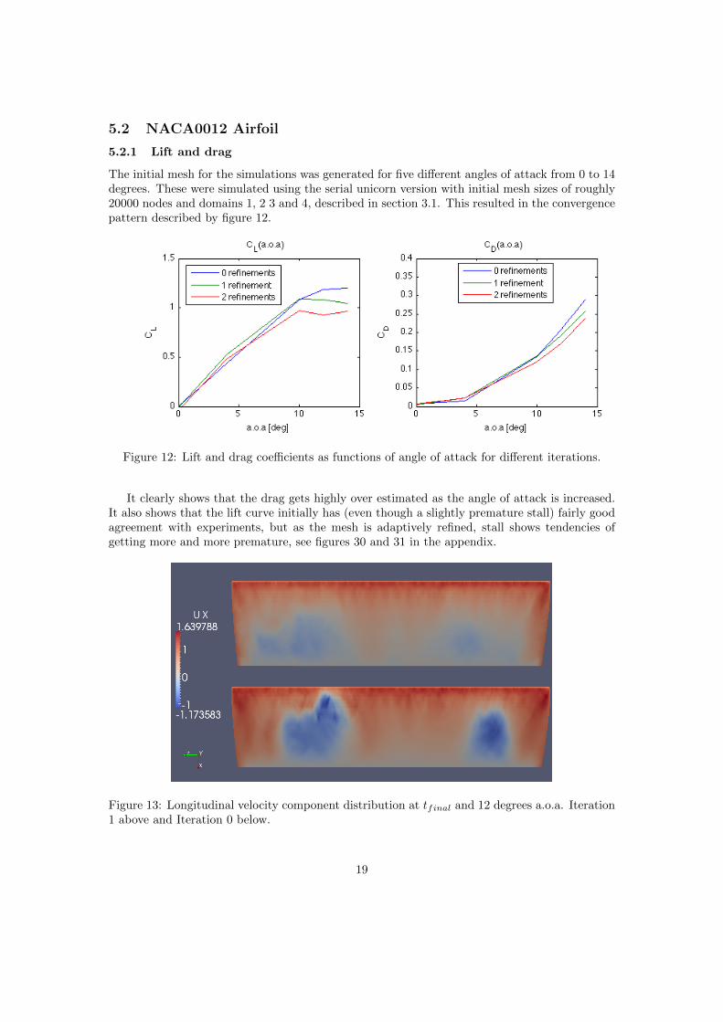
The initial mesh for the simulations was generated for five different angles of attack from 0 to 14degrees. These were simulated using the serial unicorn version with initial mesh sizes of roughly20000 nodes and domains 1, 2 3 and 4, described in section 3.1. This resulted in the convergencepattern described by figure 12.

Figure 12: Lift and drag coefficients as functions of angle of attack for different iterations.

It clearly shows that the drag gets highly over estimated as the angle of attack is increased.It also shows that the lift curve initially has (even though a slightly premature stall) fairly goodagreement with experiments, but as the mesh is adaptively refined, stall shows tendencies ofgetting more and more premature, see figures 30 and 31 in the appendix.

Figure 13: Longitudinal velocity component distribution at tfinal and 12 degrees a.o.a. Iteration1 above and Iteration 0 below.

19

As figure 13 shows, the separation is more intense for the refined mesh. This result agreeswith the lift curves but contradicts the drag curves, since more separation tends to reduce thelift and increase the drag. Therefore, it was believed that the refinement created more rapidchanges in normals, while it also was refined the wake, so that the ”vortex sausages” got moreresolved, see figure 14. Another idea was that the fact that the normals were computed from themesh might have caused problems, being slightly different from the ones of the true geometry.Furthermore it was reasoned that the leading edge might not have been resolved enough. Inorder to rule out the normal error as reason for the difference between the simulation and theexperiments, the mesh normals were exchanged for the analytical one as described in section 3.2,for the 10 degrees a.o.a. As can be seen in figure 15, this did not make a considerable change.

Figure 14: Cells marked for refinement at 12 degrees a.o.a. Iteration 1 is shown as wireframeand Iteration 0 as surface and red means marked.

Therefore more resolved meshes were used instead, which also required use of the parallelunicorn version in order for the simulations to be finished in reasonable time. Since a limitedamount of servers were available, these simulations were only made for 10, 15 and 18 degreesangle of attack. This because the larger angles were the ones with the most pronounced errorin lift and drag. The mesh size was chosen to be around 100 000 nodes, see table 1. While thiswas made, another issue was however encountered, namely the fact that using edges enforcedno slip-like conditions at the trailing edge, and therefore also creating a ”low speed bubble”around the trailing edge, see figure 16. This lead to the conclusion that edges might destroy thesolution and thus should not be used. Note that the edge/corner conditions were put there bythe software, for all edges/corners between neighboring surface elements that had an inclinationof π/6 or more.

However a new problem arised from taking them away entirely. When there were no edgesin the junction between the wing and the wind tunnel walls, jets of span wise flow appeared, seefigure 17. Though not wanted, neither of the artifacts had a major impact on the mean valueresults. The lift and drag coefficients of the cases are presented in table 5.2.1.

The results for above mentioned angles of attack and edge conditions on the wind tunnel

20

Figure 15: Lift and drag coefficient time plots for mesh normals and geometry normals.

Figure 16: Low speed bubble/stagnation on trailing edge.

walls only are presented in table 9.The reason that results from no more iterations are available (especially for 15 deg) is that at

this point in the simulation, the difference between the aerodynamic force computations betweenthe serial solver and the parallel one, pointed out in section 5.1, was discovered. Therefore, andin order to save time, another, smaller mesh was used only for 10 degrees a.o.a, with unit chordand span and wind tunnel corners in [-2,-0.5,-0.5] and [5,0.5,0.5]. This mesh was used for bothaerodynamic force computation algorithms. The resulting force coefficient plots are presented infigure 18. Here, the supercomputer results have been plotted as 8 iterations, since the uniformrefinement corresponds to at least 4 adaptive refinements.

In order to check if the results are converging towards some final result, a mesh with 800K

21

Edge boundary condition CL CDEdge conditions on all edges 1.11 0.13

No edge conditions at all 0.93 0.10No edge condition on TE only 0.93 0.11

Table 8: Lift and drag coefficients for different edge boundary conditions.

Figure 17: Span wise jet, from no edge condition at wing/wall junction. Red is high velocitymagnitude.

Figure 18: Comparison between simple, new force computation algorithm for 10 degrees a.o.afor short span wing and experiments (figures 30 and 31).

22

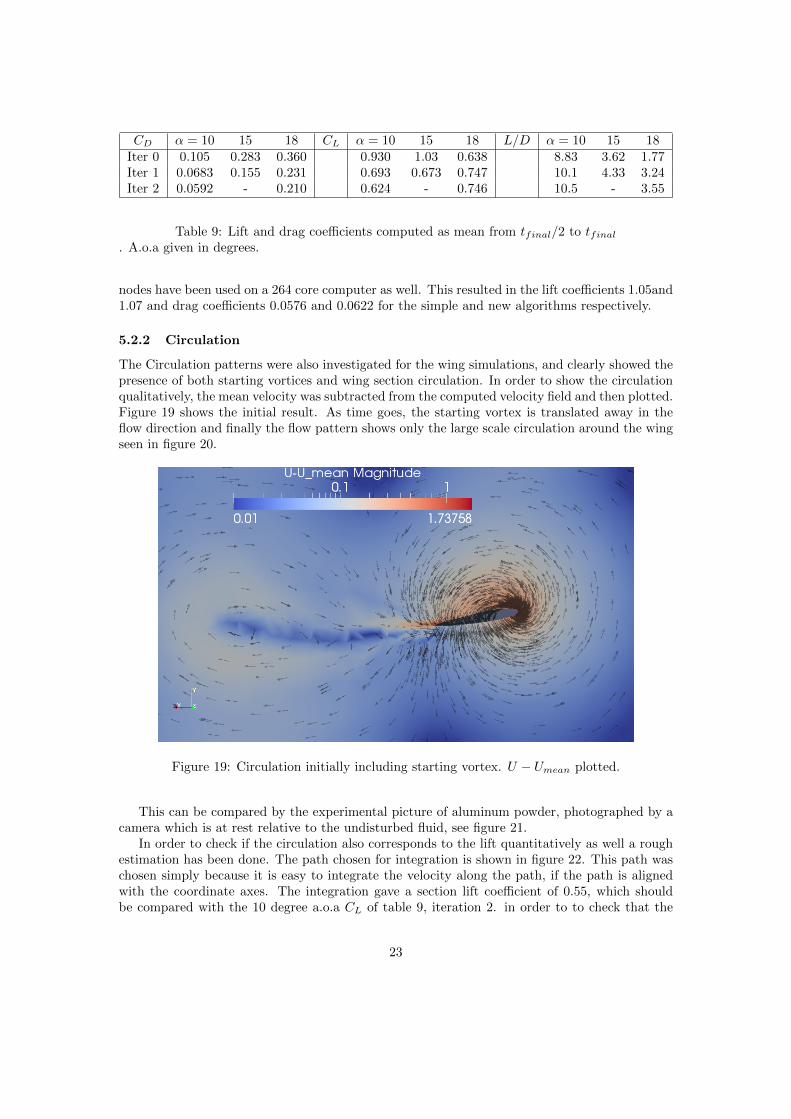
CD α = 10 15 18 CL α = 10 15 18 L/D α = 10 15 18Iter 0 0.105 0.283 0.360 0.930 1.03 0.638 8.83 3.62 1.77Iter 1 0.0683 0.155 0.231 0.693 0.673 0.747 10.1 4.33 3.24Iter 2 0.0592 - 0.210 0.624 - 0.746 10.5 - 3.55

Table 9: Lift and drag coefficients computed as mean from tfinal/2 to tfinal. A.o.a given in degrees.

nodes have been used on a 264 core computer as well. This resulted in the lift coefficients 1.05and1.07 and drag coefficients 0.0576 and 0.0622 for the simple and new algorithms respectively.

5.2.2 Circulation

The Circulation patterns were also investigated for the wing simulations, and clearly showed thepresence of both starting vortices and wing section circulation. In order to show the circulationqualitatively, the mean velocity was subtracted from the computed velocity field and then plotted.Figure 19 shows the initial result. As time goes, the starting vortex is translated away in theflow direction and finally the flow pattern shows only the large scale circulation around the wingseen in figure 20.

Figure 19: Circulation initially including starting vortex. U − Umean plotted.

This can be compared by the experimental picture of aluminum powder, photographed by acamera which is at rest relative to the undisturbed fluid, see figure 21.

In order to check if the circulation also corresponds to the lift quantitatively as well a roughestimation has been done. The path chosen for integration is shown in figure 22. This path waschosen simply because it is easy to integrate the velocity along the path, if the path is alignedwith the coordinate axes. The integration gave a section lift coefficient of 0.55, which shouldbe compared with the 10 degree a.o.a CL of table 9, iteration 2. in order to to check that the

23

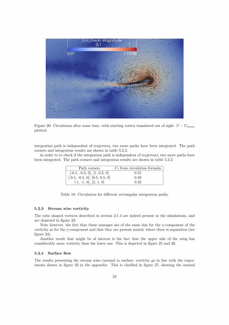
Figure 20: Circulation after some time, with starting vortex translated out of sight. U − Umeanplotted.

integration path is independent of trajectory, two more paths have been integrated. The pathcorners and integration results are shown in table 5.2.2.

in order to to check if the integration path is independent of trajectory, two more paths havebeen integrated. The path corners and integration results are shown in table 5.2.2.

Path corners Cl from circulation formula[-0.1, -0.2, 0], [1, 0.2, 0] 0.55

[-0.5, -0.5, 0], [0.5, 0.5, 0] 0.40[-1, -1, 0], [2, 1, 0] 0.23

Table 10: Circulation for different rectangular integration paths.

5.2.3 Stream wise vorticity

The tube shaped vortices described in section 2.1.4 are indeed present in the simulations, andare depicted in figure 23.

Note however, the fact that these sausages are of the same size for the x-component of thevorticity as for the y-component and that they are present mainly where there is separation (seefigure 24).

Another result that might be of interest is the fact that the upper side of the wing hasconsiderably more vorticity than the lower one. This is depicted in figure 25 and 26.

5.2.4 Surface flow

The results presenting the stream wise-/normal to surface- vorticity go in line with the exper-iments shown in figure 32 in the appendix. This is clarified in figure 27, showing the normal

24

Figure 21: Photo of aluminum powder in an airflow taken with a camera which is at rest relativeto the undisturbed flow. [12]

to surface vortices, responsible for smearing out the china clay in circular patterns and creatingwhat [5] refer to as stall cells.

Though the figures look similar to the experiments, it should be noted that these separationpatterns occur much earlier for the simulations than in the experiments. Figure 27 is takenfrom a low resolution10 degree a.o.a run with edge condition at the trailing edge. For the highresolution simulations these patterns seem to emerge at somewhat higher angles of attack (after10 but before 15 degrees). Note that the experiments showed these patterns at 15-17 degreesa.o.a [5].

5.3 Flutter plate

The flutter plate simulation was unsuccessful in the sense that stationary solutions were obtainedfor the 0 a.o.a simulations. Tries were however made for plates with large angles of attack, whichshowed oscillatory motion of the plate as it converged towards some mean deflection. Since theseresults have no experiments for comparison, they may work as a technology demonstration ratherthan as a validation of the solver. The angular and vertical displacements of the two cases canbe seen in figures 28 and 29.

25

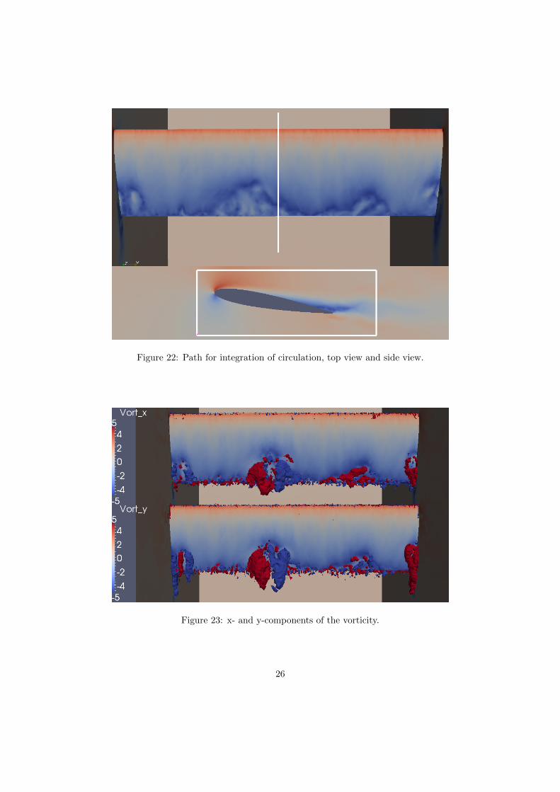
Figure 22: Path for integration of circulation, top view and side view.

Figure 23: x- and y-components of the vorticity.

26

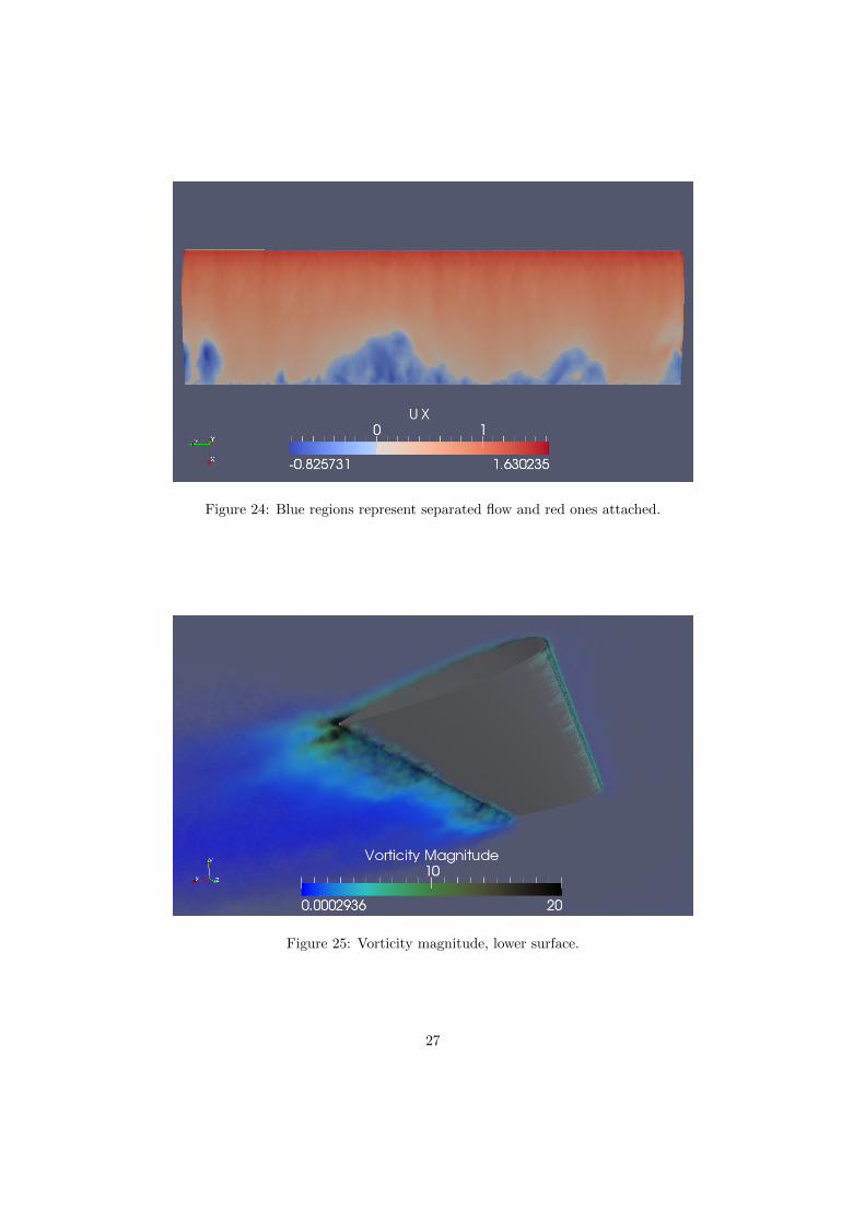
Figure 24: Blue regions represent separated flow and red ones attached.

Figure 25: Vorticity magnitude, lower surface.

27

Figure 26: Vorticity magnitude, upper surface.

Figure 27: Computed surface flow during stall. Snap shot below and 5 seconds of low opacityvelocity vectors above.

28

Figure 28: Computed vertical and angular displacements for 0 degree a.o.a plate tip.

Figure 29: Computed vertical and angular displacements for 15 degree a.o.a plate tip.

29

6 Discussion

6.1 Circulation and streamwise vorticity

Apparently Johnson and Hoffman’s theory results in both large scale circulation around thesection of a wing and a starting vortex. Furthermore, the circulation is of the right order ofmagnitude compared to the lift even though not independent of where it is integrated. Trulyremarkable however, is the fact that this is a result from inviscid computations, since the commonexplanation of generation of circulation comes from the viscous BL, and gives rise to somequestions that might need further investigation to be answered.

• Are the vortex sausages present in the computations from other state of the art softwareand can they be seen in experiments?

• Is there a way to make simplified models of airflow by connecting the x-y-plane vorticityto the chordwise circulation and create more accurate vortex lattice types of aerodynamicforce estimation methods?

• Is it possible to avoid this friction by allowing all velocity directions not crossing the surfaceat the nodes? or could it be possible to avoid by using curved elements (superparametric)?

• Why is the circulation reducing as the integration path is moved away from the wing?

• It seems, qualitatively like the streamwise vorticity mainly is present where separation ispresent. Could this be the explanation of separation rather than lift and drag?

6.2 Lift and drag

It seems like the lift coefficient converges toward the experimental values, but that drag estima-tions are too high. A list of proposed explanations is presented as follows:

• It is argued in [7] to be a result from the wind tunnel tests showing results from low Reynoldsnumber flows, and comparisons are being made between L/D for Unicorn simulations andfor full scale airliners. The author however, argues that the difference in L/D betweenthese wind tunnel tests and full scale aircraft is mainly due to wing tip vortices, fuselagedrag and drag from horizontal and vertical stabilizers. Therefore, the author suggests thatsimulations should be made for a mesh of a full scale, low speed aircraft with Unicorn.

• One proposition is that a small error in the total aerodynamic force vector direction would,as a result of the large difference between lift and drag, give a large impact on the dragbut not on the lift.

• Another proposed explanation for the difference in drag, compared to [5] is that the trailingedge and wake might need to be further resolved in order for the wake, especially close tothe wing to include smaller vortices.

• Finally, one idea for explaining the drag is that it could be a result from artificial friction,created by the velocity vector projection made by the slip condition at the nodes.

30

6.3 Edge conditions

The fact that edges seem to create no slip like conditions, could according to the author be anexplanation to the cube simulations converging towards the real drag coefficient, even thoughthe difference between edge and no edge was quite small in some wing cases. However, in orderto look closer into the validity of this explanation, the author suggests that the cube simulationsshould also be performed without edges, to see if this results in a highly different drag coefficient.Furthermore, since these simulations have been made with non zero viscosity, it would also bepreferred to try no edge in combination with zero viscosity. One way to solve the edge issueentirely could be to use a cube with filleted edges. Another example of bad influence from edgeconditions in the simulations is that this condition has in some cases been applied on the leadingedge, due to poor resolution, creating premature stall.

6.4 Geometric error

In order to avoid a too sharp leading edge creating premature stall, a lot of effort has been putinto using a mesh which is fine enough at the leading edge. This is a problem, both because ittakes a lot of time to get a satisfactory mesh and because of the fact that it is likely to resultin an unnecessarily fine mesh. Therefore it would be a large advantage if it would be possibleto use a truly coarse mesh and a geometry file that ensures the added nodes from the adaptiverefinement are placed on the actual geometry rather than in between the nodes on the mesh.

6.5 Flutter plate

The stationary solution of the scenario that in experiments has proved to generate flutter maybe a result of many reasons, and the ones the author can think of are listed below.

• The computations have been made for isotropic structure, while the experiment was madewith glass fiber-epoxy composite.

• The total force perturbations of the stationary solution might have been too small forflutter to be trigged.

• The flow part of the problem might estimate ∂CL

∂α and the aerodynamic damping in anon-conservative way. This might be a result of a too poorly resolved fluid.

This shows that the problem might be too complex for an early validation of a fluid-structureinteraction solver. An option that would probably be more efficient is to first validate theflow solver with a simpler structural model, either by using a mass-spring model or by setting aprescribed motion of the plate/wing and comparing these results with corresponding experiments.

7 Conclusions

• The Cube simulations have been very successful, showing convergence towards experimentaldrag coefficients within a few percent.

• The results presented in [6] have been reproduced with a new software framework, and liftseems to be accurate in comparison with experiments.

• In order to straighten out the argument regarding the impact from wing tips and fuselage,etcetera, a simulation should be made for a full scale aircraft.

31

• In order to give answers to the questions regarding the impact from edges creating partsof no slip like conditions, no edge simulations of the flow around a cube should be carriedout. For now, however it seems like no edges and fillets would be the best way, to avoidthe need of ad hoc edge placement.

• In order to avoid artifacts like the jet in figure 17, the use of fillets on edges, rounding themoff is proposed.

• The automatic movement of new nodes to the exact geometry at adaptive refinement isconcluded to be crucial for effective use of adaptivity and initial mesh size.

• In order to validate the flow solver for unsteady boundaries, the author recommends eitherusing a simple well tried structural model, like the pitch-plunge case, or a prescribedboundary movement like the one described by [4].

• For the fluid-structure interaction functionality to be useful for aeroelastic stability analysis,the author recommends trying some way of including perturbations that may trigger anunstable behaviour.

• One conclusion to be made however, can be drawn from [8]. This is the fact that thefluid-structure interaction version of unicorn does reproduce the results of the Hron-Turek2D benchmark problem [11] within a few percent.

32

References

[1] www.fenics.org.

[2] www.salome-platform.org.

[3] John F. Douglas, Janusz M. Gasiorek, and John A. Swaffield. Fluid mechanics, 5th edition.Ashford colour press ltd, Gosport, 2005.

[4] H. W. Forsching. Prediction of the unsteady airloads on oscillating lifting systems andbodies for aeroelastic analyses. 1978.

[5] N. GREGORY and C. L. O’REILLY. Low-speed aerodynamic characteristics of naca 0012aerofoil section, including the effects of upper-surface roughness simulating hoar frost. 1973.

[6] Johan Hoffman and Claes Johnson. Computational Turbulent Incompressible Flow. Springer-Verlag Berlin Heidelberg, 2007.

[7] Johan Hoffman and Claes Johnson. The mathematical secret of flight. 2009.

[8] M. Stockli J. Hoffman, J. Jansson. Unified continuum modeling of fluid-structure interaction.2010.

[9] Dayang Laila Abang Haji Abdul Majid and ShahNor Basri. Lco flutter of cantilevered wovenglass/epoxy laminate in subsonic flow. 2008.

[10] Chean Chin Ngo and Kurt Gramoll. Fluid mechanics - theory. http://www.ecourses.ou.edu.

[11] S. Turek and J. Hron. Proposal for numerical benchmarking of fluid-structure interactionbetween an elastic object and laminar incompressible flow. 2006.

[12] Theodore von Karman. Aerodynamics. McGraw-Hill, 1963.

33

Appendix

Figure 30: Experimental CL − α-curves. [5]

34

x ±y x ± y0.0000000 0.0000000 0.5120819 0.05216200.0005839 0.0042603 0.5362174 0.05051610.0023342 0.0084289 0.5602683 0.04876190.0052468 0.0125011 0.5841786 0.04691240.0093149 0.0164706 0.6078921 0.04498020.0145291 0.0203300 0.6313537 0.04297780.0208771 0.0240706 0.6545085 0.04091740.0283441 0.0276827 0.6773025 0.03881090.0369127 0.0311559 0.6996823 0.03667000.0465628 0.0344792 0.7215958 0.03450580.0572720 0.0376414 0.7429917 0.03232940.0690152 0.0406310 0.7638202 0.03015150.0817649 0.0434371 0.7840324 0.02798280.0954915 0.0460489 0.8035813 0.02583370.1101628 0.0484567 0.8224211 0.02371420.1257446 0.0506513 0.8405079 0.02163470.1422005 0.0526251 0.8742554 0.01763530.1594921 0.0543715 0.8898372 0.01573510.1775789 0.0558856 0.9045085 0.01391430.1964187 0.0571640 0.9182351 0.01218230.2159676 0.0582048 0.9309849 0.01054850.2361799 0.0590081 0.9427280 0.00902170.2570083 0.0595755 0.9534372 0.00761080.2784042 0.0599102 0.9630873 0.00632380.3003177 0.0600172 0.9716559 0.00516850.3226976 0.0599028 0.9791229 0.00415190.3454915 0.0595747 0.9854709 0.00328040.3686463 0.0590419 0.9906850 0.00255950.3921079 0.0583145 0.9947532 0.00199380.4158215 0.0574033 0.9976658 0.00158700.4397317 0.0563200 0.9994161 0.00134190.4637826 0.0550769 1.0000000 0.00126000.4879181 0.0536866

Table 11: NACA0012 coordinates normalized with respect to chord length.

35

Figure 31: Experimental CD − α-curves. [5]

Figure 32: Experimental china clay surface low visualization for NACA0012 at 17 degrees a.o.a.[5]

36