wood recruitment modeling in netmap
TRANSCRIPT
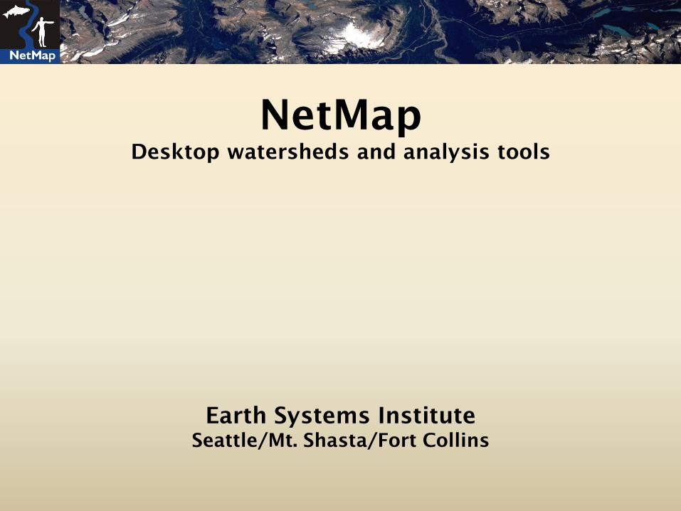
NetMap
Desktop watersheds and analysis tools
Earth Systems Institute
Seattle/Mt. Shasta/Fort Collins

A Collaborative Enterprise since 2007
-National Forests (WA, OR, NCA, AK, ID, MT)
-Forest Service Research: PSW, PNW; RMRS
-NOAA
-BLM
-EPA
-Oregon Dept. Forestry
-NGOs
-Watershed Councils
-Universities
-Private timber

Pre-fire planning
Post-fire (BAER) planning
Conservation
RestorationRoads
Forestry: Timber harvest
riparian management
Aquatic
Habitats
Applications
Climate
change

A desktop watershed is a virtual environment where landforms and physical and
biological processes are placed in context with spatial patterns of human activities
and infrastructure

NetMap in ArcMap 10/10.1
~70 tools/100+ parameters
-River Builder (create your own)
-Basic Tools
-Fluvial Morphology
-Aquatic Habitat
-Erosion
-Riparian Management
-Transportation/Energy

Current and Pending Coverage
2013/14
USFS
Region 1
½ of USFS
Region 5
EPA
Puget Sound
USFS
Region 6

NetMap Tools
Over to Sam…

Spatially Explicit Riparian Management
fish habitat distribution, debris flow risk & upslope wood
recruitment, streamside mortality wood
recruitment thermal loading
A stepwise procedurefor riparian managementplanning based on:

Example area: Lake Creek, a tributary to the Alsea River
Alsea River
Lake Creek basin (5 km2)

Step 1 – Define fish habitat distribution and quality
Define fish-bearing streams:e.g., Coho habitat (gradient < 8%; in red)

Step 2 – Define habitat distribution and quality by species
Lake creek is a moderate value Coho stream withIntrinsic Potential = 0.1 –0.5

Step 3 – Identify other species of concern (steelhead)
Lake creek is a better steelhead (than Coho) stream: IP values up to 0.8

Step 4 – Determine slope stability concerns, including landsliding
Certain areas in the Lake Creek basin are potentially unstable (in red)
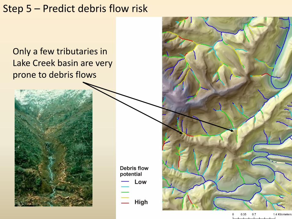
Step 5 – Predict debris flow risk
Only a few tributaries inLake Creek basin are very prone to debris flows
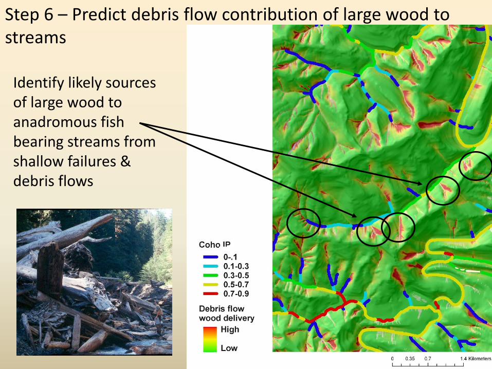
Step 6 – Predict debris flow contribution of large wood to streams
Identify likely sourcesof large wood toanadromous fishbearing streams fromshallow failures &debris flows

• Reach scale – Per 100m reach or project– For selected piece sizes – Temporally and spatially explicit– Up to 3 stands on each bank– Plots of volume and number of pieces
• Watershed scale– Temporally and spatially explicit– CE analysis of management scenarios– Based on RSWM technology– Plots and maps available
• SnapShot scale– Spatially explicit– Uses GNN tree data
Steps 7,8,9 – Evaluate effects of thinning on in-stream wood recruitment
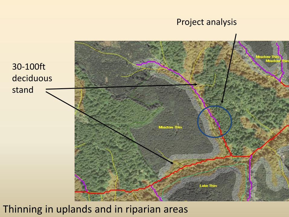
Thinning in uplands and in riparian areas
30-100ftdeciduousstand
Project analysis

Reach Scale Wood Model (RSWM)
Stream reachForest standsForest stands
Hillslope gradients
Channel width
Standwidths
Mortality types include suppression, fire, insect, disease, & wind-throw.
Bells and Whistles: channel width, stand width, hillslope gradient, bank erosion, wood decay, taper equations, thinned trees that are tipped,
and size of resulting wood pieces
Inputs: stand tables from forest growth modelsOutputs: 10 types of plots
Kozak, 1988; Bilby et al, 1999; Benda and Sias 2003; Sobota et al, 2006; Hibbs et al, 2007; and more.

RSWM Scenarios • Left bank is always no action scenario (70 m)• Right bank treatment scenarios (11) with and without a no action buffer• Double entry thin, 70 TPA: 2010, 2040• All other parameters held constant (bank erosion, channel width,
gradient, taper equations)
Right bank scenariosStand1 Stand2
No action buffer (10 m) No action (60 m)No action buffer ThinnedNo action buffer Thin & tip 5%No action buffer Thin & tip 10%No action buffer Thin & tip 15%No action buffer Thin & tip 20%Thinned (70 m)Thin & tip 5%
Thin & tip 10%Thin & tip 15%Thin & tip 20%

0
5
10
15
20
25
30
2010 2020 2030 2040 2050 2060 2070 2080 2090 2100 2110
Wo
od
Vo
lum
e (
m3
10
0 m
-1 r
eac
h)
Year
Cumulative wood volume using 2 bank scenarios, no buffer
Untreated / UntreatedUntreated/Double thinUntreated/Double thin, tip 5Untreated/Double thin, tip 10Untreated/Double thin, tip 15
0
5
10
15
20
25
30
2010 2020 2030 2040 2050 2060 2070 2080 2090 2100 2110
Wo
od
Vo
lum
e (
m3
10
0 m
-1 r
eac
h)
Year
Cumulative wood volume using 2 bank scenarios, 10 m buffer
Untreated / UntreatedUntreated/Buffer10_Double thinUntreated/Buffer10_Double thin tip 10%Untreated/Buffer10_Double thin tip 15%Untreated/Buffer10_Double thin tip 20%
The buffer reduces the effect of the thin and tip by reducing loss of wood. But in the long term the volume of wood in the stream increased to close to the untreated scenario.
Scenarios with tipped trees produce higher volumes of wood in the reach than untreated or thinned stands for most of the time simulated.

Total volume of cumulative wood over time(sorted by increasing volume)
Total cumulative wood
Volume (m3 100 m-1 reach)
(percent change from reference )
Untreated/Double thin 156 (-42%)
Untreated/Double thin, tip 5% 232 (-14%)
Untreated/Buffer10_Double thin 243 (-10%)
Untreated/Untreated (reference condition) 271
Untreated/Double thin, tip 10% 284 (5%)
Untreated/Buffer10_Double thin tip 10% 288 (6%)
Untreated/Buffer10_Double thin tip 15% 299(10%)
Untreated/Buffer10_Double thin tip 20% 305 (13%)
Untreated/Double thin, tip 15% 324 (20%)
Tree tipping from thinning operations combined with riparian buffers offer the highest volumes of wood loadings

Step 8. Watershed Scale Wood Model
Stand tables from forest growth models (FVS, Organon, Zelig) pre-processed in RSWM
Tabular data integrated with GIS: stream segments,
stands, and DEM
Generate output:plots and maps

Watershed area = 5 km2
Coho and steelhead habitat
Km
Step 11 - Consider ‘cumulative effects’ of thinning at watershed scale(example, wood recruitment) – a key part of the analysis (not complete)
Parameters: variable age stands, variable thinning timing and location over 30 years, numerous stream segments, 100 years

Stand treatments – thin to 70 TPA from the bottom(47% of watershed thinned)

Stand treatments – no action buffer & thin(39% of watershed thinned)

Spatial distributed sources of wood volume, year 2055
Difference between wood volumes, thinned and no action buffers, year 2055.
v2055th_dif
Difference in wood volume
More wood no action buffer
zero difference
More wood thinned buffer
Stands
Alt_NOth_B
No Thin
No Thin
Thin
Thin
0 50 10025 Meters

Wood volume by time (m3 100m-1 yr-1)Thinned 2015
No action buffer Thinned buffer
1995: high initial mortality – result of FVS model parameters2015: thinned2025 – 2085: no action buffer produces more wood2095+ : thinned buffer scenario produces more wood
Only one stand had data to 2295, others ended at 2195, hence the low values after 2195

Wood volume by piece size and time (m3 100m-1 yr-1), thinned 2015No action buffer Thinned buffer
Thinned buffers resulted in a 15% decrease in wood volume

Percent changes in wood volume by piece size (cm) from no action to thinned buffer
Decrease in wood of smaller sizes
Increase in wood of larger sizes
-40 -20 0 20 40
0
10
35
60
80
Total

Small reduction in the smallest volumes of wood in storage w/thinning, increases in larger volumes of stored wood w/thinning
Compare the cumulative distributions of total wood storage, 1000 stream segmentsover 100 years – not available.

Step 9. SnapShot wood model (coming summer 2013)
GNN wood data: snags / longevity value (10.66 or 20 yrs.)
Average height,
diameter, mortality
Probability of falling into the
stream by random fall
direction
Distance to stream, slope, channel width
Ohrmann and Gregory, 2002; Benda and Sias, 2003; Parish et al, 2010
Map of reaches with
wood by pieces or volume

SnapShot wood model – data availability(coming summer 2013)

Applications for land management
– Multi-scale: reach or project scale v. watershed scale management and analysis;
– Enables spatially variable approach and analysis;
– Designs for riparian treatments –thinning, buffers, habitat;
– Designs for mitigation,
enhancement, tree tipping

Step 10. Modeling stream thermal
loading for varying forest conditions

Examine the effect of thinning on thermal loading

Evaluate buffer designs
Both sides

NetMap: Thermal Tool Interface

Thermal tool sensitivity analysis:difference between fully vegetated and bare earth
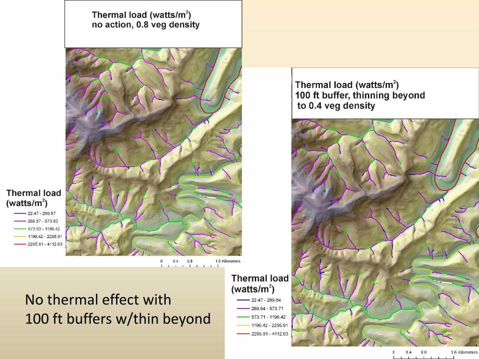
No thermal effect with100 ft buffers w/thin beyond

NetMap Tools
Back to Lee …

Step 12 - Assemble the pieces and design forest management andwatershed restoration (one hypothetical example)
Add road restorationactivities to reduce mass wasting & surface erosion

Spatially variable fire frequency based on landscape position

Step 13: (optional): Run forest fire simulation models (withtopographic dependency on fire frequency) to predict spatiallyheterogeneous nature of forest ages, including in riparian zones
On average, over time, approx.14% of the total length offirst-order streams arepredicted to have forestsless than 50 yrs old
Drops to 8% along largervalley floors
(distribution > 200 yrsnot shown)
Results from southwestWashington(GTR-101-CD, 2002)

NetMap
Community Digital Watersheds & Shared Analysis Tools
Earth Systems Institute
www.earthsystems.net
Seattle/Mt. Shasta/Fort Collins
www.netmaptools.org