Working Paper Series

This paper can be downloaded without charge from: http://www.richmondfed.org/publications/economic_research/working_papers/index.cfm

Recourse and Residential Mortgage Default: Theory

and Evidence from U.S. States�

Andra C. Ghent and Marianna Kudlyaky

Federal Reserve Bank of Richmond Working Paper No. 09-10R

June 10, 2010

Abstract

We analyze the impact of lender recourse on mortgage defaults theoretically and

empirically across U.S. states. We study the e¤ect of state laws regarding de�ciency

judgments in a model where lenders can use the threat of a de�ciency judgment to deter

default or to shorten the default process. Empirically, we �nd that recourse decreases

the probability of default when there is a substantial likelihood that a borrower has

negative home equity. We also �nd that, in states that allow de�ciency judgments,

defaults are more likely to occur through a lender-friendly procedure, such as a deed

in lieu of foreclosure.

JEL: E44, G21, G28, K11, R20. Key Words: De�ciency Judgment. Foreclosure.

Negative Equity. Residential Mortgage Default. Recourse.

�We thank Brent Ambrose, Larry Cordell, Jane Dokko, Kris Gerardi, Je¤rey Gunther, Bob Hunt, NedPrescott, Peter B. Ritz, Brent Smith, Jay Weiser, Paul Willen, and participants at the ALEA AnnualMeeting, FRB Richmond, FRB Philadelphia, the Federal Reserve System Committee on Financial Structureand Regulation Meeting, the FDIC / FHFA Symposium on Assessing Mortgage Default Risk, the Univ. ofWisconsin - FRB Atlanta HUML Conference, and the Wegmans Conference at the Univ. of Rochester forhelpful comments. This paper has bene�ted from conversations with Patricia Antonelli, Roger Bear, ChrisCauble, Dale Cottam, Craig Doyle, Charles Just, Doug Hanoy, Bob Kroker, Lester Leu, Michael Manniello,Kenneth McFadyen, Richard Rothfuss, Roman Sysuyev, Louis Vitti, Dave Weibel, and Randall Wharton.Anne Stilwell provided excellent research assistance. We thank Mark A. Watson at FRB Kansas City forassistance with the LPS data. The views expressed here do not necessarily re�ect those of the FederalReserve Bank of Richmond or the Federal Reserve System. All errors and omissions are ours alone.

yGhent: Zicklin School of Business, Baruch College; email andra.ghent@baruch.cuny.edu; phone 646-660-6929. Kudlyak: Research Department, FRB Richmond; email marianna.kudlyak@rich.frb.org; phone804-697-8791.

I. Introduction

The recent surge in defaults on residential mortgages has renewed interest in under-

standing borrowers�decisions of whether to default and what factors in�uence that decision.

One factor of interest is the recourse permitted to lenders. In some U.S. states, recourse

in residential mortgages is limited to the value of the collateral securing the loan. In other

U.S. states, the lender may be able to collect on debt not covered by the proceedings from

a foreclosure sale by obtaining a de�ciency judgment. Large increases in defaults in states

that severely restrict lender recourse, such as California and Arizona, raise the question of

whether allowing lenders more recourse substantially deters default.

Existing literature usually models the default decision as a borrower exercising a default

option when it is �in the money�, i.e., when the borrower is in a negative equity situation.1

Thus, if the lender has no recourse, even borrowers who do not experience a change in their

income or mortgage payments, but who �nd themselves having substantial negative equity

in their homes, will default on their mortgages. However, allowing the lender recourse to

assets other than the mortgaged property lowers the value of the default option and thus

reduces the borrower�s incentive to default.

In this paper we explore the di¤erences in recourse law across states to study the e¤ect of

recourse on residential mortgage default. We examine both how much recourse deters default

and to what extent it changes how borrowers default. The e¤ect of recourse on default is

not clear a priori. De�ciency judgments may be rare in practice. This may be because it is

often costly and time-consuming for a lender to pursue and collect on a de�ciency judgment.

Alternatively, the mere threat of a de�ciency judgment may deter default, implying few

de�ciency judgments in practice. Therefore, the lack of de�ciency judgments observed may

not be a good indicator of their in�uence on borrowers�behavior.

We present a model in which lenders can use the threat of a de�ciency judgment to get

the borrower to agree to expedite the default process or to deter default altogether. The

borrower �rst decides how to default and then, based on the expected payo¤ from default,

decides whether to default. In the subgame perfect equilibrium of the model, lenders rarely

1See, for example, Kau, Keenan, Muller, and Epperson (1992) and Deng, Quigley, and Van Order (2000).

1

pursue de�ciency judgments. However, allowing lenders recourse deters default in many

situations. Further, recourse has an impact on how default happens: when the lender has

recourse, defaults that do occur are likely to lead to smaller losses to lenders.

We investigate the e¤ect of recourse on default empirically using a large sample of

residential mortgages from the Lender Processing Services Inc. (LPS) Applied Analytics

database. Our empirical �ndings are as follows. First, recourse has a negative e¤ect on the

probability of default when there is a substantial likelihood that a borrower has negative

home equity (at high values of the default option). Second, the magnitude of the deterrent

e¤ect of recourse on default varies with the appraised value of the mortgaged property at

origination. The e¤ect is signi�cant only for higher-appraised properties. In particular, we

�nd that, for properties appraised at less than $200,000 (at origination, in real 2005 terms),

there is no di¤erence in the probability of default across recourse and non-recourse states.

At the mean value of the default option at the time of default and for homes appraised

at $500,000 to $750,000, borrowers in non-recourse states are more than twice as likely to

default as borrowers in recourse states. We also �nd that recourse deters default on loans

held privately. We cannot reject the hypothesis that recourse does not have an e¤ect on

loans held by government sponsored enterprises (GSEs). Third, allowing the lender recourse

increases the likelihood that default occurs by a more lender-friendly method, such as a deed

in lieu, rather than foreclosure.

Our �nding that recourse deters some borrowers from defaulting indicates that a non-

negligible portion of U.S. mortgage default is in fact strategic rather than involuntary,

whereby borrowers have no choice but to default because of liquidity constraints. This

�nding contrasts with the view that mortgage defaults are primarily driven by shocks to the

borrower�s ability to pay (see, for example, Foote, Gerardi, and Willen [2008]). Based on

their analysis of a rich dataset from Massachusetts, Foote, Gerardi, and Willen (2008) con-

clude that negative equity is not a su¢ cient condition for default. However, Massachusetts is

a recourse state, and analyzing data only from recourse states gives an incomplete picture of

the role of negative equity in the borrower�s default decision. As our �ndings show, the bor-

rower�s decision to default in recourse states is substantially less sensitive to negative equity

than in non-recourse states. Guiso, Sapienza, and Zingales (2009) and Bhutta, Dokko, and

2

Shan (2010) also �nd that at least some portion of default is not due to liquidity constraints.

To our knowledge, ours is the �rst study looking at di¤erences in how borrowers default.

Earlier work by Clauretie (1987), Jones (1993), and Ambrose, Capone, and Deng (2001) has

also looked empirically at di¤erences in defaults across states.2 Clauretie (1987) estimates a

linear regression model of aggregate state default rates and �nds that whether or not a state

permits a de�ciency judgment does not signi�cantly a¤ect the state�s default rate. Jones

(1993) looks at evidence from Alberta, which does not permit de�ciency judgments, and

British Columbia, which permits de�ciency judgments, and �nds that defaults in Alberta

are more likely to be due to deliberate defaults, rather than due to trigger events in the

borrower�s life. Ambrose, Capone, and Deng (2001) include a dummy variable for whether

a state allows a de�ciency judgment in their study of the determinants of mortgage default

in a sample of Federal Housing Administration (FHA) loans originated in 1989. Because

the principal of FHA loans is guaranteed by the FHA, FHA lenders cannot seek a de�ciency

judgment such that FHA loans may be particularly poorly suited to studying the e¤ect of

recourse on default behavior.

Ambrose, Buttimer, and Capone (1997) study theoretically the e¤ect of de�ciency judg-

ments on default and �nd that the probability of default is a decreasing function of the

probability of obtaining a de�ciency judgment. Our theoretical model builds on Ambrose,

Buttimer, and Capone (1997) by exploring the interaction of recourse laws and the lengthi-

ness of the foreclosure process but incorporates more fully the lender and borrower�s incen-

tives and the negotiation that goes on between them which determines how the borrower

terminates the mortgage.

The remainder of the paper proceeds as follows: The next section describes how lender

recourse varies across the U.S. states. Section 3 presents a model of the negotiation between

borrowers and lenders as a function of lender recourse, default costs, and homeowner equity.

In section 4 we describe our data and variables. We present our empirical results in section

5. Section 6 concludes.2Pence (2006) does not directly study how recourse a¤ects default rate; however, she looks at di¤erences

in average loan size in census tracts that span two states and �nds that the average loan size is smaller instates with more defaulter-friendly foreclosure laws.

3

II. Foreclosure Law and Default

A. Foreclosure Law Across the U.S. States

States vary in the statutes governing how much recourse the lender has in the event the

lender forecloses on the property and the proceeds from the foreclosure sale are not su¢ cient

to cover the borrower�s debt. States also di¤er in how long it takes the lender to foreclose.

In most states, the lender may obtain a de�ciency judgment to cover the di¤erence

between the balance owed and the value of the home in the event the lender must foreclose

in a negative equity situation. In states that permit de�ciency judgments, various restrictions

often apply. Usually, the lender must credit the borrower�s account for the fair market value

of the property rather than the foreclosure sale price. The fair market value restriction is

likely present because the lender is often the only bidder at the foreclosure sale (see, for

example, Brueggeman and Fisher [2008]). In the absence of such a restriction, the lender

could pro�t from a foreclosure by bidding an arti�cially low price. In addition to lowering

the likely recovery from a de�ciency judgment, such restrictions sometimes imply that the

lender must incur substantially higher legal costs and more time in pursuing a de�ciency.

The increase in costs and time depends on state statutes governing the determination of

fair market value. In some states, a single appraiser determines fair market value. In other

states, such as Minnesota, fair market value must be determined by a jury. Finally, states

di¤er in how easy it is for the borrower to contest the fair market value of the property.

Lenders have less recourse in practice in states that require lenders to go through a

lengthy judicial foreclosure process, rather than a quicker non-judicial foreclosure process,

to obtain a de�ciency judgment. In other states, such as Idaho and Nebraska, there is

a relatively short period in which the lender can �le. In some states, substantial personal

property or wages are exempt from collection on the de�ciency. Finally, in Ohio and Iowa, the

lender has a relatively short period in which to collect on the de�ciency after the foreclosure

sale.

In states that allow de�ciency judgments, a borrower retains the option to declare

bankruptcy and have some portion or all of the de�ciency judgment discharged. As White

(1998) reports, prior to the 2005 bankruptcy reform, most unsecured debts were discharged

4

in bankruptcy regardless of whether the borrower �led under chapter 7 or under chapter 13.

Furthermore, �ling for bankruptcy had a low pecuniary cost before the 2005 act such that

the major cost of �ling for bankruptcy was reduced availability of credit. In chapter 7 �lings,

it continues to be the case that de�ciency judgments are completely discharged and, if the

chapter 7 �ling is concurrent with a foreclosure, the lender loses the right to a de�ciency

judgment. In chapter 13 �lings, the lender may pursue a de�ciency judgment. Following the

2005 bankruptcy reform, however, borrowers with incomes above the state median income

usually must �le under chapter 13, rather than chapter 7, which might make it more di¢ cult

to discharge a de�ciency judgment for high income borrowers.

A few states explicitly forbid de�ciency judgments on most homes (Arizona and Oregon)

or on purchase mortgages. In other states, the restrictions on de�ciency judgments are so

onerous that it is highly impractical for the lender to pursue a judgment in the vast majority

of cases, which makes the state e¤ectively non-recourse. Table 1 summarizes the extent

of recourse the lender has in each state and the time it takes the lender to complete the

foreclosure process if the borrower does not contest the foreclosure. We classify Alaska,

Arizona, California, Iowa, Minnesota, Montana, North Carolina (purchase mortgages), North

Dakota, Oregon, Washington, and Wisconsin as non-recourse states.3

Our classi�cation of states is similar to that of the USFN (America�s Mortgage Banking

Attorneys). The states we classify as non-recourse are the same as those for which the USFN

(2004, pp. 5-5 - 5-7) indicates that a de�ciency judgment is either not available or for which

getting one is impractical. However, we classify purchase mortgages in North Carolina as

non-recourse since state law prohibits de�ciency judgments on purchase mortgages and we

treat South Dakota as a recourse state. We usually were able to speak with at least one

foreclosure attorney in each state where the amount of recourse in practice was unclear or

the statutes were di¢ cult to understand.3Appendix A describes the foreclosure and de�ciency judgment procedures in the U.S. states. We use

the foreclosure timelines from the National Mortgage Servicer�s Reference Directory (2004) published by theUSFN (America�s Mortgage Banking Attorneys).

5

B. Types of Default

In this paper, we use the term default to refer to a default that ends with the borrower

vacating the home. In practice, lenders usually view litigiously foreclosing as a last resort in

the event the borrower defaults and will often try to recover a portion of principal through

other means before resorting to foreclosure.4 Furthermore, lenders have a strong interest in

foreclosing quickly on the property even when the lender does choose to exercise the option

to foreclose.5

Lenders prefer to avoid foreclosures, especially contested foreclosures, for several rea-

sons. First, properties depreciate substantially when the borrower is in default. Second, the

property usually sells at a distressed value in a foreclosure sale. Third, lenders may incur

negative publicity and reputation costs among other prospective borrowers from forcibly

removing a borrower from his or her home. For instance, Campbell, Giglio, and Pathak

(2009) �nd that a foreclosure reduces the value of the home by approximately 28%. The

depreciation rate is faster when a property is in default because the borrower has no incen-

tive to adequately maintain the property and thus may deliberately accelerate the property�s

depreciation.

There are at least three lender-friendly ways by which a borrower can default: a short

sale, a voluntary conveyance, or simply agreeing not to contest the foreclosure. In a short

sale, the borrower �nds a buyer for the property who pays a purchase price that is less than

the full balance of the debt owed. Usually in a short sale, the lender agrees to waive his right

to a de�ciency in exchange for the borrower selling the property and remitting the proceeds

to the lender. Occasionally, the lender may only agree to waive his right to a de�ciency if the

borrower agrees to give the lender a lump sum payment in addition to the sale proceedings.

In a voluntary conveyance, the borrower hands over the deed to the property to the

lender. In the most common voluntary conveyance, a deed in lieu, the lender forgives the debt

owed in exchange for the deed. In addition to eliminating the risk of the lender pursuing a

de�ciency judgment, a deed in lieu may a¤ect a borrower�s future access to credit less severely

4See, for example, Larsen, Carey, and Carey (2007), Brueggeman and Fisher (2008), and Ling and Archer(2008).

5This view was also prevalent among the foreclosure attorneys to whom we spoke.

6

than if the lender must forcibly evict the borrower (Larsen, Carey, and Carey [2007]). The

bene�t to the lender is that, in addition to getting the property back more quickly, the

lender�s legal costs are lower and the deed in lieu of foreclosure �can be bene�cial to the

lender�s public image and to the public perception of the property�(Ling and Archer [2008]).

However, a voluntary conveyance carries some risks to the lender. First, if the borrower

declares bankruptcy within one year of a deed in lieu, the court may declare the conveyance

improper. In such a case, the lender�s claim becomes an unsecured claim on the borrower�s

assets and, in the case of the borrower �ling under chapter 13, on the borrower�s future

income, which will generally give the lender a worse payo¤. Second, a voluntary conveyance

does not cut o¤ any subordinate liens on the property the way a foreclosure does.

Finally, a borrower may simply agree to what is known as a �friendly foreclosure�. In

a friendly foreclosure, the borrower agrees to not contest the foreclosure and to submit to

the jurisdiction of the court regarding leaving the property and cooperating with the lender.

The main bene�t of this option is that the lender gets the property back more quickly

relative to a contested foreclosure. This takes more time than a voluntary conveyance but

is less time-consuming than a standard foreclosure (Brueggeman and Fisher [2008]). A

friendly foreclosure may be preferable to the lender as it cuts o¤ any subordinate interests

that may exist on the property and protects the lender if the borrower subsequently declares

bankruptcy (Ling and Archer [2008]). The bene�ts to the borrower from a friendly foreclosure

relative to a more standard foreclosure are similar to those from a short sale and a deed in

lieu: the lender usually agrees to waive his or her right to a de�ciency judgment.

Subsequent to a voluntary conveyance, the property becomes real estate owned (REO),

i.e., the lender owns the property. A property can also become REO subsequent to a fore-

closure sale if the lender acquires the property by virtue of being the only bidder.

III. A Model of the Default Decisions

In this section, we present a static model to study the e¤ect of recourse on default. In

the model, default refers to a situation that ends in the borrower vacating the home. The

model predicts that allowing lenders recourse changes both default rates and the method of

default even if lenders seldom actually pursue de�ciency judgments in equilibrium.

7

A. The Economic Environment

The borrower makes two decisions regarding default: whether to default on the mortgage

and how to default if she defaults. The borrower�s decision of whether to default on the

mortgage depends on the costs of default which, in turn, depend on whether the lender will

pursue a de�ciency. Default can happen through a litigious foreclosure or a lender-friendly

default. A lender-friendly default is a termination method that results in the lender getting

the property back more quickly and in better condition, which we view as being akin to

a friendly foreclosure, a deed in lieu of foreclosure, or a short sale. We combine lender-

friendly default outcomes into one event in the model for simplicity and because the lender

and borrower have similar incentives in both situations. The central issue is whether the

borrower cooperates with the lender or contests the foreclosure, not the precise method of

mortgage termination. Herein, we refer to that outcome as a lender-friendly default. In the

event of a foreclosure, the lender has the opportunity to seek a de�ciency judgment.

We assume that 1) the lender can get the property back more quickly if the borrower

agrees to default through a lender-friendly method; 2) the borrower receives free rent during

the default period; 3) the lender agrees to waive a de�ciency judgment if the borrower

defaults through a lender-friendly method; 4) at the foreclosure sale, the lender recovers less

than the fair market value of the property; 5) the lender recovers a greater fraction of the

fair market value if the default is lender-friendly; 6) if the lender sues for a de�ciency, the

borrower receives credit for the fair market value of the home; 7) the lender must pay a �xed

cost to pursue a de�ciency judgment; and 8) the borrower must pay a �xed cost to default.

Assumption (2) follows Ambrose, Buttimer, and Capone (1997). Assumption (4) is

based on widespread evidence that properties depreciate substantially more rapidly during

foreclosure and the lender is often the only bidder at a foreclosure sale (see, for example,

Campbell, Giglio, and Pathak [2009]). Thus, the lender cannot recover the fair market value

of the property in foreclosure. Assumption (6) is consistent with most states� foreclosure

laws requiring the borrower to receive credit for the fair market value of the home in any

de�ciency judgment. The �xed cost in assumption (8) refers to the search costs, transactions

costs, and the cost of being excluded from credit markets that the borrower must face if she

8

defaults.

In the model, we assume the lender will not agree to a loan modi�cation. This as-

sumption stems from empirical evidence that loan modi�cations are rare prior to the end

of our sample (December 2008). For example, Adelino, Gerardi, and Willen (2009) �nd

that only 3% of seriously delinquent loans receive payment-reducing modi�cations; see also

White (2009) for evidence on the infrequency of modi�cations. See Adelino, Gerardi, and

Willen (2009) and Piskorski, Seru, and Vig (2009) for discussions of why residential mortgage

modi�cations are rare during our sample period.

B. The Model

Consider a borrower with a home worth H and a balance owed on her mortgage of M ,

H < M , i.e., the borrower has negative equity. The borrower decides whether to terminate

her mortgage or whether to continue making payments. The mortgage can be terminated

in one of three ways: 1) the borrower and lender agree to a lender-friendly default (LFD),

2) the borrower and lender agree to a foreclosure and the lender does not seek a de�ciency

judgment (F), or 3) the lender forecloses with a de�ciency judgment (FDJ). If the lender

pursues a de�ciency judgment, he cannot recover his collateral for � periods. � is exogenous

to the model and determined by states�foreclosure laws.

The lender�s payo¤s from each of these possibilities are as follows. The payo¤ from no

default, XND, is

XND =M;

whereM is the unpaid mortgage balance. The lender�s payo¤ from a lender-friendly default,

XLFD, is

XLFD = �LFDH;

where H is the value of the home at the time the borrower announces he will default and

�LFD is the recovery rate in the event of a lender-friendly default, 0 < �LFD < 1.

The lender�s payo¤ from a foreclosure with no de�ciency judgement, XF , is

XF =

�1

1 + r

���FH;

9

where �F is the lender�s recovery rate in the event of a foreclosure, 0 < �F < �LFD < 1, and

r is the discount rate. The lender�s payo¤ from a foreclosure with a de�ciency judgement,

XFDJ :

XFDJ =

�1

1 + r

�� ��FH + � [M �H + cDJ ]� cDJ

�;

where � is the recovery rate, i.e., the fraction of the expected present value the lender collects

on the de�ciency, and cDJ is a �xed cost the lender must pay to pursue a de�ciency judgment.

The lender can recover a portion � of cDJ from the borrower.

The borrower receives free rent h (a fraction of the home value akin to the rent-price

ratio) in any period in which she is in default but has not been foreclosed upon. Once the

borrower either agrees to a lender-friendly default or gets foreclosed upon, she must pay the

default cost. If the borrower defaults, she incurs a �xed cost cD.

The borrower�s payo¤s are thus as follows. The payo¤ in case of no default, YND, is

YND = H �M:

The borrower�s payo¤ from a lender-friendly default, YLFD, is

YLFD = �cD:

The borrower�s payo¤ from a foreclosure with no de�ciency judgement, YF , is

YF =

�Xk=0

�1

1 + r

�khH �

�1

1 + r

��cD:

and the borrower�s payo¤ from a foreclosure with de�ciency judgement, YFDJ , is

YFDJ =

�Xk=0

�1

1 + r

�khH �

�1

1 + r

��[� (M �H + cDJ) + cD] :

C. Model Solution

Figure 1 illustrates the sequential problem the lender and the borrower solve. The

borrower and the lender choose the strategy that delivers the highest payo¤. The game has

10

a unique pure strategy equilibrium; we do not consider mixed strategy equilibria.

The model can be solved recursively. The borrower solves the lender�s problem and

ascertains, conditional on default, whether the lender will pursue a de�ciency judgment and

whether the lender will accept a lender-friendly default. After comparing the payo¤s, the

borrower makes her decisions regarding how to default and whether to default.

In a non-recourse situation, the option of default through a foreclosure with de�ciency

judgement is eliminated from both the lender�s and the borrower�s payo¤ set. In this situa-

tion, the solution to the game is simple: the borrower always defaults through a foreclosure.

The reason is that the borrower gets a higher payo¤ from being foreclosed upon since she

enjoys free rent during the foreclosure period.6

If the lender has the legal right to pursue recourse, and then either the borrower or

the lender opts for foreclosure, the lender decides whether to pursue a de�ciency judgment.

Conditional on foreclosing, the lender will pursue a de�ciency judgement if XFDJ > XF , i.e.,

if

(1)�

1� �

�M

H� 1�� cDJH

> 0.

That is, the lender will foreclose with a de�ciency judgment if the value of the de�ciency

exceeds the recoverable portion of the �xed costs of pursuing the judgment. In the extreme

cases where there is full recovery or the cost of pursuing a de�ciency is zero, the lender

always pursues a de�ciency judgment if the lender forecloses. At the other extreme, the

lender never pursues a de�ciency judgment if � = 0. In general, the lender is more likely to

pursue a de�ciency judgment when the expected recovery is high, when the current loan to

value is much greater than 1, and when the cost of pursuing a de�ciency judgment is small

relative to the value of the home.

If (1) does not hold, introducing recourse does not change the equilibrium outcome. In

this case, any threat on the part of the lender to pursue a de�ciency is not credible. The

solution is the same as in a non-recourse situation, i.e. the borrower defaults via foreclosure.

Thus, recourse will not change the equilibrium outcome when either the recovery rate is very

6The borrower will, in fact, enjoy free rent during any period between default and an LFD as well. Thedi¤erence the model captures is thus the di¤erence in the length of the period of free rent.

11

low or the cost of pursuing a de�ciency is high relative to the value of the property.

If (1) holds, the lender agrees to a lender-friendly default only if XLFD > XFDJ , i.e., if

(2)�LFD � (1 + r)�� �F

1� � >

�1

1 + r

�� ��

1� �

�M

H� 1�� cDJH

�.

That is, the lender agrees to a lender-friendly foreclosure if the discount on the home from

foreclosure relative to that from a lender-friendly method is larger than the present value of

the de�ciency recovered less the costs of pursuing the de�ciency relative to the home value

that cannot be recovered. Clearly, the lender will always agree to a lender-friendly default

if the lender would not pursue a de�ciency on a foreclosure.

Thus, there are three possible ways that introducing recourse can change the equilibrium

from the non-recourse equilibrium: 1) recourse deters default; 2) recourse results in a de�-

ciency judgment; 3) recourse induces a lender-friendly foreclosure. Recourse deters default

when the following two conditions are met: 1) the lender will not agree to a lender-friendly

default, i.e., if condition (2) does not hold, and 2) the borrower�s payo¤ from not defaulting

exceeds the payo¤ from a foreclosure with de�ciency judgement, i.e.,

(3) 1� MH>

�Xk=0

�1

1 + r

�kh+

�1

1 + r

�� ��

�1� M

H� cDJH

�� cDH

�.

For the lender to pursue a de�ciency judgment, the present value of what the lender will

recover from pursuing a de�ciency net of costs must exceed the higher value of the collateral

the lender recovers by agreeing to a lender-friendly default. If this is the case, the borrower

will only default if she does not have so much negative equity that the value of not defaulting

is higher than the free rents she receives less what she will have to pay back the lender from

the de�ciency judgment.

Examining conditions (2) and (3) also shows when the de�ciency judgments are actually

observed in equilibrium. If the loan-to-value is very high and � is moderate, the borrower still

bene�ts more from paying some of the de�ciency back than from not defaulting, particularly

since she also receives free rent during the foreclosure period.

The conditions under which recourse deters default also depend on how much delay

12

pursuing a de�ciency introduces into the foreclosure process. From examining (2), it is clear

that the lender is more likely to agree to a lender-friendly default when pursuing a de�ciency

would substantially delay the default process. Similarly, the deterrent e¤ect of recourse

decreases with the length of time it takes to foreclose because 1) the period of free of rent

increases, and 2) the de�ciency and �xed cost of default the borrower eventually has to pay

are discounted more heavily.

The second way that recourse changes the equilibrium outcome occurs when the recovery

on the de�ciency is su¢ ciently high that (1) holds, but is su¢ ciently low that (2) also holds.

In this situation, the lender pursues a de�ciency in the event of a foreclosure. For the

borrower to still default in this situation, it must also be the case that

�cDH> 1� M

H

and�cDH

>�Xk=0

�1

1 + r

�kh+

�1

1 + r

�� ��

�1� M

H� cDJH

�� cDH

�.

The �rst condition states that the �xed cost of default must be su¢ ciently low relative

to the amount of negative equity. The second condition states that the present value of

the de�ciency that the borrower must repay the lender must be larger than the value to

the borrower of the period of free rent and of delaying the payment of the �xed cost of

default. Thus, for even moderate values of �, introducing recourse is likely to lead to a more

lender-friendly method of default.

D. Discussion

To summarize, our model suggests that the presence of recourse will often change the

equilibrium outcome even if it does not often result in de�ciency judgments. The model

predicts that recourse will likely deter default when the expected recovery rate is high or

when the cost of pursuing a de�ciency is small relative to the value of the home. The

model also implies that, even for moderate recovery rates, borrowers will default di¤erently,

in ways that lead to lower losses for lenders, in states that allow lenders recourse. This

prediction of the model is consistent with the results of Clauretie and Herzog (1990) and

13

Crawford and Rosenblatt (1995) who �nd that, conditional upon foreclosure occurring, losses

on foreclosures are lower in states that permit de�ciency judgments. Our model suggests a

reason why, even if lenders rarely actually pursue de�ciency judgments, losses are lower in

states that permit lenders recourse.

It is worth noting that recourse laws will a¤ect how the borrower chooses to default both

in the case of voluntary defaulters (borrowers who can continue to make payments on their

mortgage if they choose to) and involuntary defaulters (borrowers who are insolvent and

unable to make payments). In our model, any borrower who is insolvent defaults such that

recourse does not deter involuntary default. In the case of involuntary defaulters, lenders

still can recover some portion of any de�ciency in most states since the lender typically has

ten years to collect on a de�ciency and can �le for a ten-year extension on that recovery,

ample time to see an improvement in a borrower�s �nancial circumstances.

Our model is static in the sense that we examine the equilibrium default decisions

conditional upon a borrower already being in a situation where she has negative equity. We

also do not consider how future house price expectations might a¤ect equilibrium outcomes.

Studying a static problem enables us to model the borrower�s and lender�s incentives in

more detail as well as to study how default occurs. The results in Corbae and Quintin

(2010) suggest that the deterrent e¤ect of recourse on default continues to hold in a dynamic

setting. Corbae and Quintin present a dynamic general equilibrium life cycle model in which

they �nd that recourse substantially reduces the foreclosure rate. Corbae and Quintin also

�nd that introducing recourse changes the home ownership rate and the cost of mortgage

credit.

In the remainder of the paper, we empirically examine how large a deterrent recourse is

to default in practice and whether defaults occur more frequently via lender-friendly methods

when state laws permit lenders recourse.

IV. Data

The data used in the study is loan-level data from LPS Applied Analytics, Inc. The

data contain information about loans on a monthly basis. The data contain information on

prime and non-prime private securitized loans, portfolio loans, and GSE loans. Appendix B

14

provides details about the variables by LPS codes.

A. Variable De�nitions

De�nition of Default.�We consider the loan as defaulted if it is terminated in one

of the following ways: by REO sale, by short sale, by payo¤ out of foreclosure, by payo¤

out of bankruptcy and serious delinquency, or by liquidation to termination. In the analysis

of the probability of default, the dependent variable takes a value of 1 in the month the

loan defaults. We drop all observations on defaulted loans subsequent to the default month.

Consequently, the dependent variable takes a value of 0 for observations in months prior to

default for defaulted loans and for all observations on loans that do not default.

Default Type.� In the analysis of whether recourse changes how default happens, we

consider only defaulted loans. We divide defaults into default by foreclosure and by a lender-

friendly method, i.e., a short sale or a deed in lieu. We de�ne a default as lender-friendly if

the loan passes directly to an REO loan or a short sale. We de�ne a default as a foreclosure

if the lender received a payo¤ out of bankruptcy or serious delinquency. Such a default is

akin to a contested foreclosure process since the borrower likely declared bankruptcy to halt

foreclosure proceedings. The default type variable takes a value of 1 if the loan defaulted

via a foreclosure and 0 otherwise.

Default Option Variables.�We de�ne the value of the default option as the proba-

bility that the borrower has negative equity in the house as in Deng, Quigley, and Van Order

(2000) and Ambrose, Capone, and Deng (2001). Since we know the balance owed on the

loan, we need only infer the distribution of individual house prices. The value of equity to

market value ki months after loan i�s origination is

Ei;t;ki =Mi;t;ki � Li;t;ki

Mi;t;ki

;

where Mi;t;ki is the market value of the property purchased at time t � ki, and Li;t;ki is the

present value of the remaining loan balance. The market value of the property is

Mi;t;ki = CiHPIi;tHPIi;t�ki

;

15

where Ci;t�ki is the cost of the property at the time of a purchase, HPIi;t is house price index

in the state where the property associated with mortgage i is located, and HPIi;tHPIi;t�ki

follows

a lognormal distribution (see Case and Shiller [1987] and Deng, Quigley, and Van Order

[2000] for details). The mean and variance of HPIi;tHPIi;t�ki

is obtained using the data available

from the O¢ ce of Federal Housing Enterprise Oversight (OFHEO).7

The value of the default option for mortgage i ki months after origination is the proba-

bility that equity is negative:

Default_Optioni;ki = Pr(Ei;t;ki < 0) = �

0@ lnLi;ki � lnMi;kiq�2HPIi;ki

1A ;where �(�) is the cumulative standard normal distribution and �2HPIi;ki is the variance of

individual house prices in the state in which the property associated with mortgage i is

located.

We also include the default option squared as in Deng, Quigley, and Van Order (2000).

Prepay Option Variables.� As a proxy for the prepayment option, we use a spread

between current market mortgage rate, rt, and the mortgage rate on the contract, r0. We use

indicator variables, rather than a continuous variable, based on the results of Kau, Keenan,

and Kim (1994) that the spread a¤ects default rates in a nonlinear fashion. Following

Ambrose, Capone, and Deng (2001), we de�ne the following dummy variables: Rate1 = 1

if r0 + 2% � rt, and 0 otherwise; Rate2 = 1 if r0 + 1% � rt < r0 + 2%, and 0 otherwise;

Rate3 = 1 if r0� 1% � rt < r0+1%, and 0 otherwise; Rate4 = 1 if r0� 2% � rt < r0� 1%,

and 0 otherwise; and Rate5 = 1 if rt < r0 � 2%, and 0 otherwise, where rt and r0 are in

percentages.

Foreclosure Timing and Recourse Variables.�We include the time it takes to

complete an uncontested foreclosure in the state in which the property is located since our

model predicts that a lengthier foreclosure process will increase defaults. Table 1 contains our

7To calculate the standard deviation of HPIi;tHPIi;t�ki

, �HPIi;ki , we use the volatility parameters A and Bprovided by OFHEO as follows:

�HPIi;ki =pAki +Bki2:

See Calhoun (1996) for the technical description of OFHEO index.

16

benchmark recourse classi�cation of states and the foreclosure timelines. We classify North

Carolina purchase mortgages as non-recourse and other mortgages on property located in

North Carolina as recourse.

Trigger Events.�We control for trigger events by including the contemporaneous

state divorce rate and the state unemployment rate. We use lagged monthly seasonally

unadjusted unemployment rates from the BLS.8

Loan Level Variables and Borrower Characteristics.� Additional variables that

we use in the empirical analysis are the age of the loan (in months), the LTV at origination,

an indicator variable that takes a value of 1 if the loan is interest only at origination, an

indicator variable that takes a value of 1 if the loan is an adjustable rate mortgage (ARM),

an indicator variable that takes a value of 1 if the loan is a jumbo, an indicator variable that

takes a value of 1 if the loan is not a purchase mortgage, and the borrower�s FICO score at

origination. We convert nominal appraisal amounts at origination into real 2005 dollars by

de�ating using the CPI excluding shelter.

Since a mortgage with an 80% LTV at origination may indicate a higher likelihood of

a second mortgage being present, we include a dummy variable that takes on a value of 1

if the LTV is exactly equal to 80%. We also include interactions of this variable with the

default option value and its square since, if an LTV of 80% makes it more likely the property

has a second mortgage, the default option value is in fact higher for these mortgages such

that it may have a stronger e¤ect on the probability of default. See Foote, Gerardi, Goette,

and Willen (2009) for empirical evidence that an LTV of exactly 80% increases the risk of

default.

B. Sample Description

We use information on loans originated between August 1997 and December 2008. Au-

gust 1997 is the �rst month that the FICO score variable is available in the data. We restrict

our analysis to �rst mortgages with constant principal and interest, ARMs, or Graduated

Payment Mortgages (GPMs) on single-family residences, townhouses, or condos. We drop all

8We do not use seasonally adjusted unemployment rates as there may be a seasonal pattern to defaultsdue to seasonal economic conditions.

17

FHA and VA loans because de�ciency judgments are prohibited on FHA loans and strongly

discouraged on VA loans (Larsen, Carey, and Carey [2007]). We also drop loans with private

mortgage insurance.

We then draw a 10% random sample from the LPS database. Our restrictions imply that

we have 85,888,286 loan-month observations. Table 2 provides a summary of the sample:

67% of our observations are on recourse mortgages and on average there is a 1% probability

that a home owner in our sample has negative equity; 7% of our observations are interest

only at origination and 20% of our observations are adjustable rate mortgages. In total, our

sample includes 2; 922; 196 loans and 43; 353 defaults.

V. The Impact of Recourse on Default

We use a probit as our benchmark model to study the e¤ect of recourse on whether

a borrower defaults. We assume that the borrower defaults if an unobserved variable x,

x = X� + ", falls below 0 where " � N (0; 1). X is a vector of variables that controls for

the borrower�s prepay and default options, other loan-level characteristics, and trigger event

variables.

As the theoretical model in section 3 shows, recourse a¤ects the borrower�s payo¤ from

defaulting. Di¤erent payo¤s from the default decision in recourse and non-recourse states

may lead to di¤erent threshold values of the default option at which the borrower defaults in

recourse and non-recourse states. Thus, to estimate the impact of recourse on the probability

of default, we model recourse in our empirical speci�cation as an interaction term between

the value of the default option and the recourse indicator variable. The recourse dummy

variable takes a value of 1 if the mortgaged property is located in a state with a provision

for recourse and 0 otherwise.

The �rst column of table 3 contains the results without recourse variables. The results

in the column illustrate the e¤ect of the prepay and default options, trigger events, and loan-

level characteristics on default when we do not control for recourse. All of the coe¢ cients

have the expected sign. Having an interest-only loan, an ARM, or a purchase mortgage raises

the probability of default. Borrowers with higher FICO scores at origination are less likely

to default while loans with a high LTV at origination are more likely to default. Finally,

18

younger loans are much more likely to default than older loans. The divorce rate has the

expected sign but is signi�cant only at the 10% level when we cluster the standard errors,

likely because there is relatively little variation across time in the divorce rate within a state.

The unemployment rate has the expected sign but becomes insigni�cant when the standard

errors are clustered.

Column 2 of table 3 contains the main result of the paper. The coe¢ cient on the

interaction term between recourse and negative equity is negative and statistically signi�cant.

The coe¢ cient on the interaction between recourse and the square of the probability of

negative equity is positive and statistically signi�cant. The negative coe¢ cient on the default

option value indicates that recourse decreases the impact of the negative equity on the

probability of default. The positive coe¢ cient on the squared term indicates that the e¤ect

decreases as the default option value increases. Because of this nonlinear e¤ect of default

option value on the probability of default, the e¤ect of recourse depends on a particular value

of the default option.

The coe¢ cient on the interaction between the default option value and the dummy for

an LTV of exactly 80% is signi�cant and positive, suggesting that properties on mortgages

with an LTV of exactly 80% are more likely to have second mortgages attached to them

and that �rst mortgages are thus more sensitive to negative equity. It is important that we

include this term to ensure that our results are not driven by the fact that there may be

more second mortgages in non-recourse states than in recourse states.9

To gauge the magnitude of the deterrent e¤ect of recourse, we evaluate the probability

of default in recourse and non-recourse states at di¤erent values of the default option. Table

4 contains the estimates of the probabilities. Columns 1 to 4 show the probabilities at the

means of the continuous variables and the modes of the dummy variables. At the mean of

the default option at the time of default, borrowers in non-recourse states are 32% more

likely to default than borrowers in recourse states. At the mean of the default option for all

observations, the probability of default is 6% higher in non-recourse states than in recourse

states. At the 90th percentile of the value of the default option for all observations, the

probability of default in non-recourse states is 2% higher. This di¤erence increases to 13%

9All our results are similar when we do not include the LTV80 variable and its interactions.

19

at the 95th percentile. The results in table 4 indicate that recourse has a deterrent e¤ect on

default at high values of the default option value, which are precisely the values associated

with default. Thus, the data allow us to reject the hypothesis that recourse has no e¤ect on

default.

In columns 3 and 4 of table 3, we present the results for two alternative speci�cations.

In column 3, we include the prepay option, the di¤erence between the contract rate and

current mortgage rates, in interactions with the probability of negative equity as in Ambrose,

Capone, and Deng (2001). The results are similar to our benchmark speci�cation, although

the log-likelihood is somewhat higher when rates are included in interactions suggesting that

including rates in levels �ts the data better.

In column 4, we explore whether our results regarding recourse are due to state-speci�c

factors by including state dummy variables.10 When we control for the state-speci�c �xed

e¤ects, the results on the e¤ect of recourse carries through: the coe¢ cient on the interaction

between recourse and the default option value is statistically signi�cant, negative, and slightly

larger in magnitude than in the benchmark speci�cation. Thus, our results regarding the

deterrent e¤ect of recourse are not driven by unobserved di¤erences between recourse and

non-recourse states.

A. Default and State Foreclosure Timelines

In column 5 of table 3, we show the e¤ect of the lengthiness of the uncontested foreclosure

process, as stated in USFN (2004), on the probability of default. In column 5 we include the

length of the uncontested foreclosure process in months for the state in which the property

is located. When we do not cluster the standard errors, states with lengthier foreclosure

processes appear to experience more defaults. However, the e¤ect becomes insigni�cant

when we cluster the standard errors by state. We also do not �nd that the lengthiness

of the foreclosure process signi�cantly a¤ects default in other speci�cations in which we

include the interaction of the foreclosure timeframe with recourse. While our model predicts

that a lengthier foreclosure process will increase the default rate in a few cases, the empirical

10We drop the divorce rate in this speci�cation as our divorce rate data are only available at the annualfrequency. Also, for some states, we only have a few divorce rate observations over the entire sample suchthat there is little variation remaining in the divorce rate after we control for state-speci�c e¤ects.

20

evidence in column 5 suggests those cases are infrequent in practice. We obtain similar results

with a speci�cation in which we include foreclosure timing by using a dummy variable that

takes on a value of 1 if the state�s uncontested foreclosure process takes more than 6 months

and 0 otherwise. Thus, we cannot reject the hypothesis that the lengthiness of the foreclosure

process has no e¤ect on the probability of default.

B. A Finer Recourse Classi�cation

In our benchmark speci�cation, we de�ne mortgages as being either recourse or non-

recourse. Our benchmark classi�cation (see table 1) de�nes a mortgage as non-recourse

if de�ciency judgments are either explicitly prohibited or impractical in the vast majority

of cases. We also consider a �ner classi�cation of non-recourse. In this speci�cation, we

categorize a mortgage as being non-recourse if it is de jure non-recourse and a mortgage

as being subject to limited recourse if the mortgage is de facto non-recourse. We de�ne

California and Montana non-purchase mortgages as well as mortgages on property in Alaska,

Iowa, Minnesota, Washington state, and Wisconsin as de facto non-recourse. We de�ne

mortgages on property in Arizona, North Dakota, and Oregon, as well as purchase mortgages

in California, Montana, and North Carolina, as de jure non-recourse.

In column 6 of table 3, we present the results from the speci�cation in which we use the

�ner recourse classi�cation: recourse (same mortgages as in the benchmark speci�cation), de

facto non-recourse, and de jure non-recourse. The omitted category is de jure non-recourse

while limited recourse is a dummy variable that takes a value of 1 if the mortgage is de facto

non-recourse and 0 otherwise. The coe¢ cient on recourse remains signi�cantly negative

and is slightly larger in magnitude than in our benchmark speci�cation. The coe¢ cient on

limited recourse is signi�cantly negative but much smaller in magnitude than the coe¢ cient

on recourse. Thus, while default is less likely if the mortgage is de facto non-recourse than

if it is explicitly non-recourse, default is more likely if the mortgage is de facto non-recourse

than if it is recourse.

21

C. Robustness

In table 5, we conduct several additional robustness exercises. First, we repeat our

analysis using only data on mortgages originated from 2005 onwards. There is some concern

that the data is of higher quality from 2005 onwards. Furthermore, a very large servicer enters

the database in 2005. Column 1 presents the results from our benchmark speci�cation but

using only data on originations from 2005 to the end of our sample. Column 2 presents the

results using our speci�cation that includes state �xed e¤ects using only data on originations

from 2005 to the end of our sample. The results are consistent with those we found using

our benchmark speci�cation.

Columns 3 to 5 of table 5 contain the additional results from the full sample. Column 3

contains the results from a speci�cation in which we include year of origination dummies. The

coe¢ cient on the interaction between the default option value and recourse is similar to that

of our benchmark speci�cation in column 2 of table 3. With 2003 as the omitted category, the

coe¢ cients on origination years from 1998 to 2001 are negative and statistically signi�cant

while the coe¢ cients on 2004, 2005, and 2006 are positive and statistically signi�cant. These

results provide some evidence that, controlling for a set of variables used in our benchmark

speci�cation, the mortgages originated in the later years of the sample, particularly from

2004 to 2006, have a higher probability of default than the mortgages originated earlier.

In columns 4 and 5 of table 5, we present proportional competing hazard models (see,

for example, Deng, Quigley, and Van Order, 2000). In our benchmark speci�cation, we use

a probit model and control for time-dependence with the time elapsed from loan origina-

tion. Thus, our benchmark speci�cation provides an estimate of the probability of the loan

defaulting in any particular month. Alternatively, we can estimate the hazard model of the

risk of default.

Generally, a mortgage can be terminated by default or prepayment such that a mortgage

is subject to two competing hazards. Column 4 contains the results (for default) from �tting

models for each termination type separately and treating failures due to a competing type

of termination as censored data. The hazard ratio on the interaction between recourse and

the default option is below 1 and highly signi�cant, indicating that recourse reduces the

22

sensitivity of default to negative equity as we found using our benchmark speci�cation.

We also estimate the two hazard functions jointly. In estimating them jointly, we assume

that the two competing hazard functions are additive. Consequently, the hazard of failure

by any termination type is a sum of the two competing processes. The observed time of

failure is the minimum time of failure of the two competing processes. Thus, at the time

of failure two survival times are observed: one for a process that corresponds to the failure

type and another one, censored, for the competing process.

We use a proportional hazard model with grouped duration data. To estimate the

competing hazards of default and prepayment, we duplicate the data using the method in

Lunn and McNeal (1995). The duplicated data set contains twice as many observations as

the original one with each new observation showing a censored observation for a competing

termination type. The censored observations are also duplicated, creating two censored ob-

servations �one for each failure type. We then de�ne a variable that identi�es two strata �

one for prepayment and one for default. The failure indicator then re�ects failures from a type

of termination corresponding to the respective stratum. We estimate the semi-parametric

Cox model including, in addition to our benchmark covariates, a strata indicator as a co-

variate, as well as interactions of the strata indicator with all covariates. Inclusion of the

strata indicator as a covariate assumes proportional baseline hazards for the two competing

types of termination while allowing the e¤ect of covariates on the hazard to di¤er.

Column 5 presents the results for default from the joint estimation of the competing

hazards model. The results from estimating competing hazards jointly are similar to those

obtained from estimating the hazards separately. The hazard ratio on the interaction between

recourse and the default option is below 1 and highly statistically signi�cant.

D. Results by Appraisal Amount

The model in section 3 predicts that the deterrent e¤ect of default on the probability

of default depends on the amount of the de�ciency judgment that a lender can actually

recover. In our empirical analysis, we proxy for the lender�s recovery rate with the appraised

value of the mortgaged property. A higher appraised value likely indicates that the borrower

has more assets that can be used by the lender to recover on the de�ciency judgment.

23

Additionally, a higher appraisal amount is more likely to be associated with higher income

since the ratio of debt to income is a key ratio in the underwriting process. Higher income

borrowers who declare bankruptcy also may have less chance to have their debt discharged

during bankruptcy proceedings. This is particularly true for borrowers considering default

after the 2005 bankruptcy reform, which usually requires borrowers above the state median

income to �le under chapter 13 rather than under chapter 7. This implies that, unlike with

poor borrowers, lenders have better recovery rates with richer borrowers. In fact, data from

the Survey of Consumer Finance indicate that there is a positive relationship between the

median value of the primary residence and �nancial (non-housing) wealth.11

Table 6 contains the results on estimating our benchmark speci�cation separately for

di¤erent values of the appraised value (real 2005 dollars) of the mortgaged property at

origination. As the results in table 6 show, recourse does not deter default for all households

in the same way. Recourse is a deterrent for default when the appraisal amount exceeds

$200,000: the coe¢ cient on the recourse interaction with the default option value and its

square are statistically insigni�cant when the appraisal amount is $200,000 or less. The

coe¢ cient on the interaction of the recourse with a linear default option term is particularly

large in the samples with appraisal amounts from $300,000 to $500,000 and from $500,000

to $750,000. For the sample with appraisal amounts of $1,000,000 or higher, the coe¢ cient

changes sign and is not statistically signi�cant.

The results of the estimation of the probability of default in the samples by appraisal

amount indicate that the e¤ect of recourse on the probability of default is mainly driven by

borrowers with mortgages on properties appraised at $200,000 and higher. To the extent that

the appraisal amount at origination proxies for the recovery rate on a de�ciency judgment,

these results indicate that recourse has a substantial deterrent e¤ect on default in cases

with higher recovery rates. Recourse does not have a statistically signi�cant e¤ect when the

recovery on a de�ciency judgment is likely to be low.

To gauge the magnitude of the deterrent e¤ect of recourse on the default probabilities,

we present estimates of the probabilities of default in recourse and non-recourse states in

11In 2007, households in the lowest quintile of �nancial (non-housing) wealth held homes worth $81,946on average while households in the second, third, fourth, and �fth quintiles of non-housing wealth held homesworth on average $118,367, $154,788, $191,208, and $318,681, respectively (in real 2004 dollars).

24

table 4. At the mean value of the default option at the time of default and for homes

appraised at $300,000 to $500,000, borrowers in non-recourse states are 81% more likely to

default than borrowers in recourse states. For homes appraised at $500,000 to $750,000,

borrowers in non-recourse states are more than twice as likely to default as borrowers in

recourse states. For homes appraised at $750,000 to $1 million, borrowers in non-recourse

states are 60% more likely to default than borrowers in recourse states.

Importantly, the size of the de�ciency judgment relative to the lender�s �xed cost of �ling

for a de�ciency is likely to be lower for low-value properties than for high-value properties.

This lowers the incentive for a lender to �le for a de�ciency judgment for low-value properties.

If the recovery rate is 100%, costs do not matter because they are recoverable. However,

if the recovery rate is less than 100%, the e¤ect of allowing the lender recourse depends

on the cost of pursuing the de�ciency judgment as well as the recovery rate; the e¤ect of

costs decreases as the recovery rate increases. As a result, the �nding that recourse does not

have a deterrent e¤ect on default for low-value properties is consistent with costs being an

important determinant of the e¤ect of allowing lenders recourse.

E. Recourse and Lender Types

Table 7 presents the results from the probit regression estimated separately for loans

held by Fannie Mae (FNMA), loans held by Freddie Mac (FHMLC), loans that are privately

held and securitized, and loans held in a bank�s portfolio. As seen in table 7, the coe¢ cient on

the interaction of the recourse dummy with the default option value is negative, sizeable, and

statistically signi�cant for privately securitized and private portfolio loans. Table 4 presents

estimates of the probabilities for recourse and non-recourse states. At the mean value of the

default option at the time of default and for securitized privately held loans, borrowers in

non-recourse states are 45% more likely to default than borrowers in recourse states while,

for privately held portfolio loans, borrowers in non-recourse states are 44% more likely to

default.12

12We also estimate our benchmark speci�cation on FHA and VA loans. Since these loans are explicitlynon-recourse in all states, we should not �nd a signi�cant negative coe¢ cient on the interaction betweenrecourse and the default option value. We �nd that the coe¢ cient on the interaction between recourse andthe default option value is positive, albeit small, for FHA and VA loans.

25

The estimation results in table 7 indicate that recourse does not have a signi�cant deter-

rent e¤ect on default for loans held by FNMA or FHMLC. The coe¢ cients on the interaction

between the default option value and recourse for the FNMA and FHMLC samples are much

smaller in magnitude than the ones for privately securitized loans and are statistically in-

signi�cant. This is true even when we consider only FNMA and FHMLC loans on properties

appraised at $200,000 or more (in real 2005 dollars), the threshold above which we found

recourse matters. We conclude that recourse has a statistically signi�cant deterrent e¤ect

on default only for privately held loans.

F. The Impact of Recourse on the Way a Borrower Defaults

We next turn to the question of how lender recourse a¤ects the way in which the borrower

defaults. We estimate a probit to determine which factors in�uence whether borrowers are

more likely to default by foreclosure. The sample is restricted to the observations for which

the default variable takes a value of 1. The dependent variable takes a value of 1 if the

default is by a foreclosure and 0 otherwise (i.e., default occurs through a deed in lieu or a

short sale).

Our model suggests that borrowers are less likely to default by litigious foreclosure in

states with recourse. We are unable to empirically distinguish between friendly foreclosures

and contested foreclosures, although our model also predicts that we should see more defaults

by friendly foreclosure than by contested foreclosure in recourse states. To test the hypothesis

that recourse in�uences how the borrower defaults, we include a recourse variable dummy as

explanatory variable for the probability of default by foreclosure. As controls, we include the

borrower�s FICO score at origination and the LTV at origination to control for unobserved

heterogeneity in the borrower�s costs of decreased access to credit or search costs. Column 1

of table 8 contains the results of the estimation. As the results indicate, recourse lowers the

probability of default by foreclosure. The estimated coe¢ cient is negative and statistically

signi�cant. In particular, the probability of default by foreclosure in recourse states is 10%

lower than the probability in non-recourse states.13

The model also predicts that the e¤ect recourse has on the way a borrower defaults

13We calculate the partial e¤ects at the mean of continuous variables and at the modes of dummy variables.

26

is in�uenced by how much recourse the lender has as well as the LTV at the time of de-

fault. However, the relationships are nonlinear. For high LTVs and high recovery rates,

the deterrent e¤ect of a de�ciency judgment is strong enough to deter default altogether.

For high LTVs and more moderate recovery rates, it is sometimes worthwhile for the lender

to pursue a de�ciency judgment and yet for the borrower to default. For moderate LTVs

and low-to-moderate recovery rates, recourse changes how the borrower defaults rather than

whether the borrower defaults.

To test whether recourse has a stronger e¤ect for higher values of the default option

value, we add the default option value and the default option value interacted with the

recourse dummy in addition to the recourse variable as the explanatory variables for the

probability of default by foreclosure. If recourse has a stronger negative e¤ect at higher

values of the default option, we expect a negative coe¢ cient on the interaction term between

recourse and the default option value. As can be seen from the results in column 2 of table

8, the negative e¤ect of recourse on the probability to default by foreclosure is stronger for

higher values of the default option. However, the e¤ect is not statistically signi�cant.

Our model suggests that the time it takes to foreclose on a home has an ambiguous

e¤ect on the share of lender-friendly defaults. On the one hand, a longer foreclosure process

makes it more likely the lender will prefer a lender-friendly default to a foreclosure and will

forgo a de�ciency judgment in favor of a deed in lieu or a short sale. However, the borrower

prefers foreclosure when she can delay the search and credit costs and receive a longer period

of free rent as a result of a lengthier foreclosure process. A priori, it is unclear what e¤ect

foreclosure timing will have on the process. To examine the e¤ect empirically, we include a

dummy variable that takes a value of 1 if the uncontested foreclosure time is less than six

months, and zero otherwise. As the results in column 3 indicate, the foreclosure timing does

not have a signi�cant e¤ect on the probability of default by the litigious foreclosure: the

partial e¤ect evaluated at the means implies an increase in probability of 2% and is far from

statistically signi�cant. The results were very similar when we included foreclosure timing

as a continuous variable rather than as a dummy variable.

Finally, we examine whether a lender�s type and the appraisal amount a¤ects the prob-

ability to default by litigious foreclosure. To examine the e¤ect of a lender�s type, we include

27

a dummy variable that takes a value of 1 if the lender is a GSE and 0 otherwise, i.e., when

the loan is privately securitized or held in a private lender�s portfolio. As can be seen from

the results in column 4, mortgages held by a GSE are no more likely to default by foreclosure

than mortgages held by private lenders.

To examine the e¤ect of the appraisal amount of the property on the probability of

default by foreclosure, we include the appraisal amount and the appraisal amount interacted

with the recourse dummy as explanatory variables. We present the estimation results in

column 5 of table 8. The coe¢ cient on the appraisal amount is positive and marginally

signi�cant. The e¤ect on the interaction term is negative but statistically insigni�cant.

G. Discussion

Our empirical �ndings shed light on the ongoing discussions about whether there is

strategic default (see, for example, Foote, Gerardi, and Willen [2008]) and whether the

default decision depends on the borrower�s income. The result that recourse deters default

indicates that at least some of the defaults in the data are strategic rather than involuntary,

whereby the borrower has no choice but to default because of liquidity constraints. Our

results indicate that at least some borrowers choose not to default when the lender has

recourse, indicating that they are capable of continuing to make payments on their mortgage.

Our results regarding the di¤erential e¤ect of recourse by the appraisal amount of the

mortgaged property indicate that at least some defaults on high and moderately priced

homes are strategic. We cannot eliminate the possibility that some of the defaults on low-

priced homes are strategic as the appraisal amount proxies for both the lender�s amount of

recourse and the borrower�s �nancial means in general. Thus, recourse may not signi�cantly

a¤ect default on low-priced homes for one of two reasons. The �rst possibility is that most

households with low-priced homes are liquidity constrained and thus default because of their

inability to carry payments. Alternatively, for low-value properties, the lender�s recovery

on a de�ciency judgment may be low in practice both because of a low recovery rate and a

relatively higher �xed cost.

The �nding that recourse has a di¤erential e¤ect on the probability of default depending

on the appraisal amount of the mortgaged property also suggests that the default decision

28

depends on the borrower�s income in recourse states. This e¤ect works via the expected

de�ciency judgment that allows the lender to claim a part of the borrower�s assets. The fact

that the default decision depends on income is relevant for policy discussions of the impact

of default on welfare (see Hatchondo, Martinez, and Sanchez [2009]).

VI. Conclusions

Our model predicts that we do not need to observe lenders frequently pursuing de�ciency

judgments to conclude that recourse alters borrowers�behavior. The threat of a de�ciency

judgment deters would-be strategic defaulters under many combinations of negative equity

and the degree of lender recourse. In other situations, if the borrower does default, then

allowing the lender to pursue a de�ciency judgment changes how the borrower defaults. In

particular, in states that allow lenders recourse, default occurs more frequently by deeds in

lieu and short sales, as recourse gives lenders better negotiating positions.

Empirically, we �nd that, in a sample of loans originated between August 1997 and

December 2008, at the mean value of the default option at the time of default, the probability

of default is 32% higher in non-recourse states than in recourse states. The deterrent e¤ect on

default is signi�cant only for borrowers with appraised property values of $200,000 or more

at origination. At the mean value of the default option at the time of default and for homes

appraised at $300,000 to $500,000, borrowers in non-recourse states are 81% more likely to

default than borrowers in recourse states. For homes appraised at $500,000 to $750,000,

borrowers in non-recourse states are more than twice as likely to default as borrowers in

recourse states while, for homes appraised at $750,000 to $1 million, borrowers in non-

recourse states are 60% more likely to default. We also �nd that recourse deters default on

loans held privately; we cannot reject the hypothesis that recourse does not have an e¤ect on

loans held by the government sponsored enterprises. Finally, we �nd that allowing lenders

recourse increases the likelihood that default occurs by a more lender-friendly method, such

as a deed in lieu of foreclosure.

Our �ndings pose a number of interesting questions. For example, what are the implica-

tions of recourse laws for welfare? Furthermore, to what extent do lenders take into account

the higher risk of default in non-recourse states at the time of mortgage origination? We

29

leave these questions for future research.

REFERENCES

Adelino, Manuel, Kristopher Gerardi, and Paul S. Willen. 2009. �Why Don�t Lenders Rene-

gotiate More Home Mortgages? Redefaults, Self-Cures, and Securitization.�Federal Reserve

Bank of Boston Working Paper 09-4.

Ambrose, Brent W., Richard J. Buttimer Jr., and Charles A. Capone. 1997. �Pricing Mort-

gage Default and Foreclosure Delay.�Journal of Money, Credit, and Banking, 29(3): 314-25.

Ambrose, Brent W., Charles A. Capone, and Yongheng Deng. 2001. �Optimal Put Exercise:

An Empirical Examination of Conditions for Mortgage Foreclosure.�Journal of Real Estate

Finance and Economics, 23(2): 213-34.

Brueggeman, William B. and Je¤rey D. Fisher. 2008. Real Estate Finance and Investments.

13th Ed. New York: McGraw-Hill Irwin.

Bhutta, Neil, Jane Dokko, and Hui Shan. 2010. �How Low Will You Go? The Depth of

Negative Equity and Mortgage Default Decisions.�Manuscript, Federal Reserve Board of

Governors.

Calhoun, Charles A. 1996. �OFHEO House Price Indexes: HPI Technical Description.�Man-

uscript, OFHEO.

Campbell, John Y., Stefano Giglio, and Parag Pathak. 2009. �Forced Sales and House

Prices.�NBER Working Paper 14866.

Case, Karl E. and Robert J. Shiller. 1987. �Prices of Single-Family Homes since 1970: New

Indexes for Four Cities.�New England Economic Review, Sept./Oct.: 45-56.

Clauretie, Terrence M. 1987. �The Impact of Interstate Foreclosure Cost Di¤erences and

the Value of Mortgages on Default Rates.�American Real Estate and Urban Economics

Association Journal, 15(3): 152-67.

30

Clauretie, Terrence M. and Thomas Herzog. 1990. �The E¤ect of State Foreclosure Laws on

Loan Losses: Evidence from the Mortgage Industry.�Journal of Money, Credit, and Banking,

22(2): 221-33.

Corbae, Dean and Erwan Quintin. 2010. �Mortgage Innovation and the Foreclosure Boom.�

Manuscript, University of Texas at Austin.

Crawford, Gordon W. and Eric Rosenblatt. 1995. �E¢ cient Mortgage Default Option Exer-

cise: Evidence from Loss Severity.�Journal of Real Estate Research, 10(5): 543-55.

Deng, Yongheng, John M. Quigley, and Robert Van Order. 2000. �Mortgage Terminations,

Heterogeneity, and the Exercise of Mortgage Options.�Econometrica, 68(2): 275-307.

Foote, Christopher L., Kristopher S. Gerardi, Paul S. Willen. 2008. �Negative Equity and

Foreclosure: Theory and Evidence.�Journal of Urban Economics, 64(2): 234-45.

Foote, Christopher L., Kristopher S. Gerardi, Lorenz Goette, and Paul S. Willen. 2009.

�Reducing Foreclosures: No Easy Answers.�NBER Macroeconomics Annual, 24, 89-138.

Guiso, Luigi, Paola Sapienza, and Luigi Zingales. 2009. �Moral and Social Constraints to

Strategic Default on Mortgages.�Manuscript, University of Chicago.

Hatchondo, Juan C., Leonardo Martinez, and Juan M. Sanchez. 2009. �Mortgage Recourse

and Foreclosure.�Manuscript, Federal Reserve Bank of Richmond.

Jones, Lawrence D. 1993. �De�ciency Judgments and the Exercise of the Default Option in

Home Mortgage Loans.�Journal of Law and Economics, 36(1): 115-38.

Kau, James B., Donald C. Keenan, and Taewon Kim. 1994. �Default Probabilities for Mort-

gages.�Journal of Urban Economics, 35(3): 278-96.

Kau, James B., Donald C. Keenan, Walter J. Muller, and James F. Epperson. 1992. �A

Generalized Valuation Model for Fixed-Rate Residential Mortgages.� Journal of Money,

Credit, and Banking, 24(3): 279-99.

Larsen, James E. with Bill Carey and Chantal Howell Carey. 2007. Real Estate. Hoboken:

Wiley.

31

Ling, David C. and Wayne R. Archer. 2008. Real Estate Principles: A Value Approach. 2nd

Ed. New York: McGraw-Hill Irwin.

Lunn, Mary and Don McNeil. 2005. �Applying Cox Regression to Competing Risks.�Bio-

metrics, 51(2), 524-32.

Pence, Karen M. 2006. �Foreclosing on Opportunity: State Laws and Mortgage Credit.�

Review of Economics and Statistics, 88(1): 177-82.

Piskorski, Tomasz, Amit Seru, and Vikrant Vig. 2009. �Securitization and Distressed Loan

Renegotiation: Evidence from the Subprime Mortgage Crisis.�Manuscript, Columbia Uni-

versity.

USFN. 2004. The National Mortgage Servicer�s Reference Directory. USFN: Tustin, CA.

White, Alan M., 2009. �Deleveraging the American Homeowner: The Failure of 2008 Volun-

tary Mortgage Contract Modi�cations�. Connecticut Law Review, 41, 1107-1132.

White, Michelle J. 1998. �Why it Pays to File for Bankruptcy: A Critical Look at the

Incentives Under US Personal Bankruptcy Law and a Proposal for Change.�The University

of Chicago Law Review, 65(3): 685-732.

32

33

Mean Std. Dev. 5th Percentile 95th PercentileRecourse 0.67 0.47 0 1Default Option (Probability of Negative Equity) 0.010 0.063 0 0.021Rate 1 0.015 0.121 0 0Rate 2 0.153 0.360 0 1Rate 4 0.080 0.271 0 1Rate 5 0.033 0.177 0 0Divorce Rate 3.82 0.87 2.60 5.10Lagged Unemployment Rate 5.07 1.14 3.30 7.00Fico Score at Origination 723 61 611 799Interest Only (at Origination) Dummy 0.067 0.250 0 1Jumbo Dummy 0.090 0.287 0 1ARM Dummy 0.196 0.397 0 1LTV Ratio at Origination 67 16 33 80Natural Log of Loan Age 3.09 0.87 1.39 4.22Purpose Type Dummy 0.649 0.477 0 1Foreclosure Timing (in months) 6.30 3.25 2 12LTV 80 Dummy 0.14 0.35 0 1Appraisal Amount (at Origination) 308,043 303,093 82,000 750,000Number of Loans 2,922,196Number of Defaults 43,353

Table 2: Summary Statistics

Notes: Recourse is a dummy variable that takes a value of 1 if the property is in a recourse state, 0 otherwise; for North Carolina,recourse takes a value of 1 if the loan is not a purchase mortgage, 0 otherwise. The rate variables control for the differencebetween the current mortgage rate and the contract rate. Purpose Type Dummy takes a value of 1 if the loan is not a purchasemortgage, 0 otherwise. LTV80 Dummy takes a value of 1 if the loan­to­value at origination is 80%.

34

Table 3: Recourse and the Probability of Default(1) (2) (3) (4) (5) (6)

1.06 1.97 1.97 1.99 1.98 2.32(0.25) (0.19) (0.22) (0.20) (0.17) (0.21)­1.18 ­2.22 ­2.81 ­2.17 ­2.23 ­2.83(0.22) (0.21) (0.27) (0.21) (0.20) (0.27)

­1.52 ­1.51 ­1.65 ­1.55 ­1.86(0.35) (0.35) (0.30) (0.31) (0.36)1.57 1.33 1.82 1.60 2.17

(0.43) (0.47) (0.37) (0.40) (0.46)­0.68(0.20)1.19(0.24)

0.13 0.13 0.12 0.13 0.13 0.13(0.02) (0.02) (0.02) (0.02) (0.02) (0.02)0.98 0.57 0.87 0.58 0.57 0.53

(0.30) (0.19) (0.20) (0.14) (0.19) (0.19)­1.81 ­1.40 ­1.74 ­1.31 ­1.40 ­1.35(0.50) (0.30) (0.30) (0.26) (0.30) (0.30)­0.359 ­0.350 ­0.359 ­0.350 ­0.350(0.027) (0.025) (0.024) (0.025) (0.025)­0.311 ­0.306 ­0.317 ­0.306 ­0.306(0.035) (0.033) (0.032) (0.033) (0.033)0.326 0.327 0.337 0.328 0.327

(0.011) (0.011) (0.008) (0.010) (0.010)0.444 0.451 0.465 0.451 0.451

(0.014) (0.015) (0.013) (0.014) (0.015)­2.418(1.121)­2.210(0.492)0.796

(0.053)0.906

(0.093)0.023 0.023 0.024 0.025 0.022

(0.014) (0.014) 0.013 (0.014) (0.015)0.008 0.007 0.015 ­0.054 0.006 0.007

(0.018) (0.020) (0.019) (0.015) (0.017) (0.021)­0.263 ­0.264 ­0.348 ­0.264 ­0.264 ­0.264(0.014) (0.015) (0.021) (0.015) (0.015) (0.015)0.195 0.187 0.111 0.187 0.188 0.186

(0.023) (0.022) (0.023) (0.021) (0.021) (0.022)0.046 0.027 ­0.019 0.021 0.028 0.027

(0.020) (0.017) (0.018) (0.014) (0.017) (0.017)0.313 0.310 0.375 0.289 0.310 0.310

(0.014) (0.012) (0.008) (0.009) (0.012) (0.012)

­

­

­

­

Default Option Sq. *Recourse ­

Rate 1 ­

Default Opt. *Limited RecourseDefault Opt. Sq. *Limited Recourse

ForeclosureTiming

Default Option

Default OptionSquaredDefault Option *Recourse ­

No RecourseDummies Benchmark Rates in

InteractionsState

Dummies

­

Rate 5 ­

Default Option *Rate 1 ­ ­

Rate 2 ­

Rate 4 ­

Divorce Rate

­

­ ­

Default Option *Rate 2 ­ ­ ­ ­

­

­

Lagged Unemp Rate

Fico Score atOrigination

­

Default Option *Rate 5 ­ ­ ­ ­

Default Option *Rate 4

Interest OnlyDummy

Jumbo Dummy

ARM Dummy

Finer RecourseClassification

LTV80

LTV80 * DefaultOptionLTV80 * DefaultOption Sq.

35

Table 3 (Continued) : Recourse and the Probability of Default(1) (2) (3) (4) (5) (6)

0.009 0.010 0.013 0.010 0.010 0.010(0.001) (0.001) (0.001) (0.001) (0.001) (0.001)0.078 0.077 0.065 0.087 0.078 0.077

(0.005) (0.005) (0.006) (0.007) (0.005) (0.005)­0.097 ­0.099 ­0.099 ­0.113 ­0.099 ­0.096(0.020) (0.021) (0.021) (0.020) (0.021) (0.021)

0.003(0.007)

­2.75 ­2.78 ­2.35 ­2.28 ­2.80 ­2.78(0.13) (0.13) (0.17) (0.12) (0.16) (0.13)

% Defaults 0.050% 0.050% 0.050% 0.050% 0.050% 0.050%Log ps. likelihood ­311,161 ­310,662 ­318,205 ­308,237 ­310,649 ­310,621Pseudo R­squared 16.46% 16.59% 14.57% 17.24% 16.59% 16.60%Number of obs. 85,888,286 85,888,286 85,888,286 85,888,286 85,888,286 85,888,286

Ln Loan Age

StateDummies

ForeclosureTiming

LTV Ratio atOrigination

Purpose TypeDummy

No RecourseDummies

­ ­ ­

Benchmark Rates inInteractions

­

Notes: The dependent variable in the probit is a binary variable that takes a value of 1 if the loan defaults in that month, 0otherwise. Default Option is the probability that the borrower has negative home equity. LTV80 takes a value of 1 if the loanhas an LTV of exactly 80%, 0 otherwise. The rate variables control for the difference between the current mortgage rate andthe contract rate. Purpose Type Dummy takes a value of 1 if the loan is not a purchase mortgage, 0 otherwise. Standarderrors are in parentheses. The coefficients and standard errors for Fico Score at Origination show the effect of a 100 pointincrease in the FICO score. Standard errors are clustered by state. Coefficients in bold font are significant at the 5% level. %Defaults is the percentage of observations that are defaults.

Finer RecourseClassification

­

Constant

Foreclosure Timing

36

Table 4: Estimated Default Probabilities in Recourse and Non­Recourse States

(1) (2) (3) (4)

Default option value 6.08% 1.00% 0.29% 2.07%Non­Recourse Def. Prob. 0.1801% 0.0088% 0.0083% 0.0095%Recourse Def. Prob. 0.1361% 0.0083% 0.0082% 0.0084%Ratio NR/R 132% 106% 102% 113%

Default option value 6.09% 0.84% 0.23% 1.28%Non­Recourse Def. Prob. 0.1750% 0.0069% 0.0066% 0.0072%Recourse Def. Prob. 0.1263% 0.0065% 0.0065% 0.0066%Ratio NR/R 139% 106% 102% 109%

Default option value 8.84% 1.14% 0.24% 2.01%Non­Recourse Def. Prob. 0.2141% 0.0048% 0.0045% 0.0052%Recourse Def. Prob. 0.1185% 0.0044% 0.0044% 0.0044%Ratio NR/R 181% 111% 102% 120%

Default option value 10.12% 1.57% 0.32% 4.00%Non­Recourse Def. Prob. 0.1721% 0.0043% 0.0039% 0.0053%Recourse Def. Prob. 0.0756% 0.0036% 0.0037% 0.0034%Ratio NR/R 228% 120% 104% 156%

Default option value 8.54% 1.30% 0.17% 2.55%Non­Recourse Def. Prob. 0.0818% 0.0039% 0.0035% 0.0043%Recourse Def. Prob. 0.0512% 0.0036% 0.0035% 0.0037%Ratio NR/R 160% 109% 101% 119%

Default option value 6.41% 2.21% 2.47% 11.40%Non­Recourse Def. Prob. 0.3306% 0.0231% 0.0235% 0.0413%Recourse Def. Prob. 0.2283% 0.0196% 0.0196% 0.0196%Ratio NR/R 145% 118% 120% 210%

Default option value 10.16% 2.55% 2.80% 15.37%Non­Recourse Def. Prob. 0.0807% 0.0211% 0.0215% 0.0448%Recourse Def. Prob. 0.0558% 0.0189% 0.0191% 0.0257%Ratio NR/R 144% 111% 113% 174%

Value of Default OptionAt Time of

DefaultAll Loans

Benchmark Specification

By Appraisal Amount (Real, 2005$)

At Mean ofDefault

At Mean At 90thpercentile

At 95thpercentile

$500,000 to $750,000

$750,000 to $1,000,000

$200,000 to $300,000

$300,000 to $500,000

Private Securitized

Private Portfolio

By Investor Type

Note: The benchmark specification is specification (2) from table 3. The probabilities areestimated at the modes for dummy variables and means for the variables other than thedefault option value and default option value squared. In column 1, we estimate theprobabilities at the modes of dummy variables and the means of all variables at the timeof default for defaulted loans. Ratio is the ratio of the probabilities in non­recourse andrecourse states.

37

Table 5: Robustness

(1) (2) (3) (4) (5)Coefficients

1.53 1.27 1.47 1.057 1.060(0.20) (0.10) (0.19) (0.002) (0.003)­1.84 ­1.46 ­1.80 0.999 0.999(0.18) (0.12) (0.18) (0.000) (0.000)­1.94 ­1.53 ­1.60 0.958 0.958(0.43) (0.29) (0.36) (0.002) (0.003)2.18 1.79 1.70 1.000 1.000

(0.48) (0.34) (0.43) (0.000) (0.000)0.16 0.14 0.12 1.562 1.571

(0.02) (0.02) (0.02) (0.020) (0.030)0.12 0.08 0.42 1.014 1.008

(0.19) (0.14) (0.23) (0.003) (0.004)­0.75 ­0.47 ­1.11 1.000 1.000(0.31) (0.25) (0.36) (0.000) (0.000)­0.040 ­0.016 ­0.285 0.279 0.274(0.05) (0.05) (0.03) (0.023) (0.035)­0.402 ­0.426 ­0.275 0.324 0.302(0.035) (0.034) (0.02) (0.010) (0.016)0.333 0.338 0.321 2.857 2.985

(0.012) (0.011) (0.01) (0.040) (0.066)0.430 0.460 0.425 3.877 4.103

(0.012) (0.013) (0.01) (0.070) (0.118)0.060 0.031 1.071 1.069

(0.022) (0.015) (0.006) (0.010)­0.005 ­0.115 0.016 1.100 1.079(0.021) (0.008) (0.019) (0.005) (0.008)­0.260 ­0.267 ­0.274 0.992 0.993(0.016) (0.018) (0.013) (0.000) (0.000)0.136 0.131 0.145 1.802 1.794

(0.020) (0.018) (0.015) (0.027) (0.042)0.070 0.013 0.031 1.074 1.084

(0.018) (0.030) (0.017) (0.017) (0.026)0.277 0.216 0.260 2.840 2.881

(0.012) (0.018) (0.008) (0.039) (0.062)

Rate 5

Rate 2

Rate 4

Benchmark State Dummies

­

Coefficients

Default OptionSquaredDefault Option *RecourseDefault Option Sq. *Recourse

Full Sample

Hazard RatiosCompeting

Hazards, SeparateEst.

CompetingHazards,Joint Est.

Year ofOriginationDummies

Default Option

2005­2008 Sample

LTV80

LTV80 * DefaultOptionLTV80 * DefaultOption Sq.

Rate 1

Interest Only Dummy

Jumbo Dummy

ARM Dummy

Divorce Rate

Lagged Unemp Rate

Fico Score atOrigination

38

Table 5 (Continued) : Robustness

(1) (2) (3) (4) (5)Coefficients

0.011 0.011 0.010 1.035 1.032(0.002) (0.002) (0.001) (0.001) (0.001)0.161 0.217 0.135 0.224 0.130

(0.020) (0.026) (0.020) (0.004) (0.001)­0.154 ­0.173 ­0.097 0.602 0.698(0.017) (0.019) (0.021) (0.007) (0.012)­3.09 ­2.14 ­3.07(0.17) (0.12) (0.14)

% Defaults 0.105% 0.105% 0.050%Log ps. likelihood ­180,901 ­178,135 ­308,656 ­559,643 ­12,033,972Pseudo R­squared 15.0% 16.3% 17.1%Number of obs. 25,828,688 25,828,688 85,888,286 85,888,286 68,559,958

Constant

Ln Loan Age

Purpose TypeDummy

Full Sample

Hazard RatiosCompetingHazards,Joint Est.

LTV Ratio atOrigination

State DummiesYear of

OriginationDummies

CompetingHazards, Separate

Est.Benchmark

Coefficients

2005­2008 Sample

Notes: The dependent variable in the probit (columns 1­3) is a binary variable that takes a value of 1 if the loandefaults in that month, 0 otherwise. Default Option is the probability that the borrower has negative home equity.LTV80 takes a value of 1 if the loan has an LTV of exactly 80%. The rate variables control for the differencebetween the current mortgage rate and the contract rate. Purpose Type Dummy takes a value of 1 if the loan isnot a purchase mortgage, 0 otherwise. Standard errors are in parentheses. The coefficients and standard errors forFico Score at Origination show the effect of a 100 point increase in the FICO score. Columns 4 and 5 presenthazard ratios from the estimated proportional hazard semiparametric models; standard errors are clustered byloan. The results in column 4 are from hazard functions for grouped data estimated separately, treating thecompeting hazard as censored. The results in column 5 are from the joint estimation of competing hazardfunctions for grouped data. Standard errors are clustered by state for the probit models. Coefficients in bold fontare significant at the 5% level. % Defaults is the % of observations that are defaults.

­ ­

39

1.97 0.99 1.22 2.18 2.27 2.25 2.24 1.71(0.19) (0.34) (0.36) (0.20) (0.23) (0.20) (0.22) (0.33)­2.22 ­1.79 ­1.14 ­2.45 ­2.55 ­2.86 ­2.49 ­2.22(0.21) (0.61) (0.44) (0.25) (0.25) (0.27) (0.29) (0.40)­1.52 0.18 ­0.61 ­1.76 ­2.28 ­2.81 ­1.67 1.26(0.35) (0.36) (0.39) (0.30) (0.36) (0.44) (0.82) (1.16)1.57 ­0.20 0.31 1.95 2.44 3.66 1.22 ­5.30

(0.43) (0.76) (0.48) (0.34) (0.44) (0.60) (1.23) (2.65)0.13 0.05 0.08 0.13 0.19 0.21 0.20 0.06

(0.02) (0.01) (0.01) (0.01) (0.01) (0.01) (0.02) (0.04)0.57 2.64 0.86 0.75 0.29 ­0.56 ­1.02 ­0.04

(0.19) (0.92) (0.39) (0.45) (0.21) (0.12) (0.21) (0.23)­1.40 ­16.11 ­2.44 ­1.59 ­1.14 0.39 0.85 ­0.14(0.30) (5.08) (0.66) (0.97) (0.32) (0.20) (0.28) (0.33)­0.350 ­0.200 ­0.274 ­0.325 ­0.354 ­0.547 ­0.353 ­0.203(0.025) (0.098) (0.049) (0.036) (0.046) (0.069) (0.080) (0.066)­0.306 ­0.182 ­0.227 ­0.314 ­0.325 ­0.487 ­0.371 ­0.282(0.033) (0.031) (0.023) (0.037) (0.048) (0.043) (0.090) (0.052)0.327 0.233 0.259 0.321 0.387 0.399 0.515 0.471

(0.011) (0.016) (0.014) (0.018) (0.024) (0.014) (0.056) (0.030)0.451 0.364 0.372 0.468 0.519 0.604 0.696 0.699

(0.015) (0.025) (0.021) (0.019) (0.025) (0.031) (0.068) (0.050)0.023 0.017 ­0.015 0.025 0.067 0.104 0.061 0.019

(0.014) (0.024) (0.018) (0.016) (0.021) (0.025) (0.027) (0.032)0.007 0.046 0.017 ­0.012 ­0.024 ­0.026 ­0.040 ­0.022

(0.020) (0.021) (0.020) (0.018) (0.016) (0.020) (0.025) (0.024)­0.264 ­0.206 ­0.279 ­0.291 ­0.291 ­0.292 ­0.266 ­0.280(0.015) (0.020) (0.013) (0.012) (0.018) (0.026) (0.021) (0.026)0.187 0.010 0.146 0.206 0.202 0.231 0.209 0.175

(0.022) (0.035) (0.023) (0.018) (0.011) (0.017) (0.029) (0.051)0.313 0.291 0.325 0.344 0.330 0.206 0.195 0.102

(0.014) (0.014) (0.015) (0.018) (0.019) (0.016) (0.033) (0.041)0.009 0.006 0.009 0.009 0.013 0.015 0.012 0.013

(0.001) (0.001) (0.000) (0.001) (0.001) (0.002) (0.003) (0.001)0.078 0.039 0.080 0.096 0.106 0.101 0.069 0.076

(0.005) (0.005) (0.005) (0.009) (0.014) (0.019) (0.019) (0.020)­0.097 ­0.050 ­0.084 ­0.108 ­0.154 ­0.145 ­0.086 ­0.043(0.020) (0.016) (0.016) (0.022) (0.031) (0.023) (0.023) (0.027)

% Defaults 0.050% 0.115% 0.048% 0.039% 0.046% 0.050% 0.034% 0.027%Log ps. likelihood ­311,161 ­55,730 ­96,082 ­57,104 ­63,350 ­26,487 ­5,866 ­4,121Pseudo R­sq 16.46% 11.52% 14.62% 17.72% 20.45% 20.36% 18.29% 14.55%Number of obs. 85,888,286 7,076,266 26,973,983 20,004,481 19,840,252 7,675,467 2,370,213 1,947,624

Default Option

All < $100,000 $100,000 to$200,000

Table 6: Recourse and the Probability of Default by Appraisal Amount (Real, 2005 $)$500,000 to

$750,000$750,000 to$1,000,000

>$1,000,000

$200,000 to$300,000

$300,000 to$500,000

Rate 4

Rate 5

Divorce Rate

Default OptionSquaredDefault Option *RecourseDefault Option Sq.* Recourse

Rate 1

LTV80 * DefaultOptionLTV80 * DefaultOption Sq.

Notes: The dependent variable in the probit is a binary variable that equals 1 if the loan defaults in that month, 0 otherwise. The benchmarkspecification is specification (2) from table 3. Default Option is the probability that the borrower has negative home equity. LTV80 takes a valueof 1 if the loan has an LTV of exactly 80%, 0 otherwise. The rate variables control for the difference between the current mortgage rate and thecontract rate.The results for Fico Score at Origination show the effect of a 100 point increase. Purpose Type Dummy takes a value of 1 if the loanis not a purchase mortgage, 0 otherwise. % Defaults is the percentage of observations that are defaults. Standard errors (clustered by state) inparentheses. All regressions include a constant.

LTV80

ARM Dummy

LTV Ratio atOrigination

Ln Loan Age

Purpose TypeDummy

Lagged UnempRateFico Score atOriginationInterest OnlyDummy

Rate 2

40

Table 7: Recourse and the Probability of Default by Investor Type

Appraisal Appraisal>$200,000 >$200,000

1.97 1.65 2.14 1.99 2.16 2.10 1.90(0.19) (0.25) (0.23) (0.27) (0.21) (0.18) (0.18)­2.22 ­1.59 ­2.36 ­2.38 ­2.56 ­2.56 ­1.71(0.21) (0.33) (0.27) (0.31) (0.31) (0.21) (0.17)­1.52 ­0.10 ­0.82 ­0.16 0.07 ­2.08 ­1.15(0.35) (0.34) (0.46) (0.37) (0.33) (0.41) (0.31)1.57 ­0.26 1.00 ­0.33 ­0.85 2.29 1.07

(0.43) (0.50) (0.58) (0.50) (0.87) (0.51) (0.37)0.13 0.05 0.06 0.07 0.10 0.15 0.17

(0.02) (0.01) (0.02) (0.01) (0.02) (0.02) (0.01)0.57 0.71 0.59 0.85 0.79 0.27 0.39

(0.19) (0.29) (0.17) (0.18) (0.20) (0.23) (0.19)­1.40 ­1.67 ­1.29 ­1.83 ­1.59 ­0.97 ­1.19(0.30) (0.27) (0.25) (0.47) (0.49) (0.38) (0.37)­0.350 ­0.121 ­0.122 ­0.165 ­0.237 ­0.448 ­0.270(0.025) (0.038) (0.050) (0.073) (0.110) (0.031) (0.059)­0.306 ­0.166 ­0.157 ­0.144 ­0.153 ­0.414 ­0.308(0.033) (0.019) (0.021) (0.023) (0.035) (0.033) (0.041)0.327 0.259 0.296 0.244 0.285 0.285 0.397

(0.011) (0.018) (0.021) (0.018) (0.039) (0.012) (0.015)0.451 0.423 0.487 0.481 0.560 0.353 0.632

(0.015) (0.023) (0.042) (0.029) (0.058) (0.011) (0.027)0.023 0.004 0.002 0.010 0.024 0.030 0.026

(0.014) (0.023) (0.016) (0.018) (0.015) (0.017) (0.019)0.007 0.025 0.011 0.022 0.002 0.004 0.014

(0.020) (0.025) (0.025) (0.020) (0.020) (0.018) (0.023)­0.264 ­0.307 ­0.327 ­0.273 ­0.284 ­0.232 ­0.182(0.015) (0.014) (0.011) (0.016) (0.018) (0.015) (0.028)0.187 0.205 0.278 0.307 0.332 0.130 0.231

(0.022) (0.048) (0.046) (0.053) (0.059) (0.023) (0.030)0.027 ­0.127 ­0.089 ­0.155 ­0.118 ­0.047 ­0.004

(0.017) (0.073) (0.078) (0.060) (0.064) (0.020) (0.022)0.310 0.147 0.167 0.080 0.094 0.280 0.261

(0.012) (0.014) (0.017) (0.028) (0.042) (0.010) (0.021)0.010 0.011 0.012 0.010 0.010 0.009 0.008

(0.001) (0.001) (0.001) (0.001) (0.001) (0.001) (0.001)0.077 0.088 0.095 0.124 0.125 0.075 0.125

(0.005) (0.007) (0.011) (0.009) (0.012) (0.008) (0.007)­0.099 0.017 0.003 0.063 0.037 ­0.163 ­0.082(0.021) (0.013) (0.022) (0.013) (0.035) (0.017) (0.014)

% Defaults 0.050% 0.0190% 0.0113% 0.0142% 0.0096% 0.165% 0.0585%Number of obs. 85,888,286 37,577,506 21,452,670 22,688,658 12,897,217 17,196,843 7,460,381

PrivatePortfolioAll All

Default Option

AllFannie Mae (FNMA) Freddie Mac (FHMLC) Private

Securitized

Default OptionSquaredDefault Option *RecourseDefault Option Sq. *Recourse

LTV80

Fico Score atOrigination

Interest Only Dummy

Rate 1

Rate 2

Rate 4

Rate 5

Purpose TypeDummy

Notes: Dependent variable in the probit is a binary variable that equals 1 if the loan defaults in that month, 0 otherwise. The benchmarkspecification is specification (2) from table 3. Default Option is the prob. that the borrower has negative home equity. LTV80=1 if the loanhas an LTV of exactly 80%, 0 otherwise. Rate variables control for the difference between the current mortgage rate and the contract rate.The results for Fico Score show the effect of a 100 point increase. Purpose Type Dummy = 1 if the loan is not a purchase mortgage, 0otherwise. % Defaults is the % of observations that are defaults. Std. errors (clustered by state) in parentheses. All regressions include aconstant.

LTV80 * DefaultOptionLTV80 * DefaultOption Sq.

Jumbo Dummy

ARM Dummy

LTV Ratio atOrigination

Ln Loan Age

Divorce Rate

Lagged Unemp Rate

41

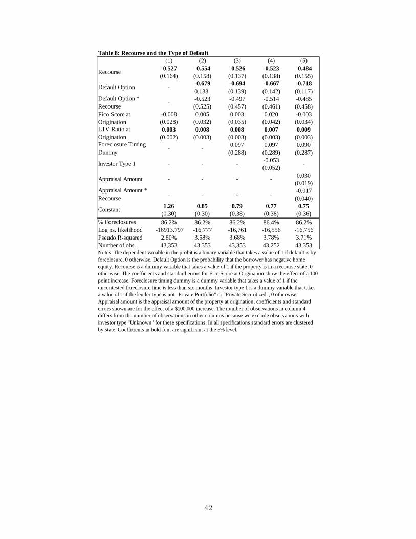
Table 8: Recourse and the Type of Default(1) (2) (3) (4) (5)

­0.527 ­0.554 ­0.526 ­0.523 ­0.484(0.164) (0.158) (0.137) (0.138) (0.155)

­0.679 ­0.694 ­0.667 ­0.7180.133 (0.139) (0.142) (0.117)­0.523 ­0.497 ­0.514 ­0.485(0.525) (0.457) (0.461) (0.458)

­0.008 0.005 0.003 0.020 ­0.003(0.028) (0.032) (0.035) (0.042) (0.034)0.003 0.008 0.008 0.007 0.009

(0.002) (0.003) (0.003) (0.003) (0.003)0.097 0.097 0.090

(0.288) (0.289) (0.287)­0.053(0.052)

0.030(0.019)­0.017(0.040)

1.26 0.85 0.79 0.77 0.75(0.30) (0.30) (0.38) (0.38) (0.36)

% Foreclosures 86.2% 86.2% 86.2% 86.4% 86.2%Log ps. likelihood ­16913.797 ­16,777 ­16,761 ­16,556 ­16,756Pseudo R­squared 2.80% 3.58% 3.68% 3.78% 3.71%Number of obs. 43,353 43,353 43,353 43,252 43,353Notes: The dependent variable in the probit is a binary variable that takes a value of 1 if default is byforeclosure, 0 otherwise. Default Option is the probability that the borrower has negative homeequity. Recourse is a dummy variable that takes a value of 1 if the property is in a recourse state, 0otherwise. The coefficients and standard errors for Fico Score at Origination show the effect of a 100point increase. Foreclosure timing dummy is a dummy variable that takes a value of 1 if theuncontested foreclosure time is less than six months. Investor type 1 is a dummy variable that takesa value of 1 if the lender type is not "Private Portfolio" or "Private Securitized", 0 otherwise.Appraisal amount is the appraisal amount of the property at origination; coefficients and standarderrors shown are for the effect of a $100,000 increase. The number of observations in column 4differs from the number of observations in other columns because we exclude observations withinvestor type "Unknown" for these specifications. In all specifications standard errors are clusteredby state. Coefficients in bold font are significant at the 5% level.

­

­

­

­

­

­

­

­

­

­

­

­

­

Recourse

Default Option

Default Option *RecourseFico Score atOrigination

Appraisal Amount *Recourse

Constant

LTV Ratio atOriginationForeclosure TimingDummy

Investor Type 1

Appraisal Amount

­

­­

42

Figure 1: Model Description

No Default Default

Borrower{Bnd;Lnd}

Lender­FriendlyDefault Foreclosure

F, no DJ F, DJ

Agree F, no DJ F, DJ

{Blfd; Llfd} {Bf; Lf} {Bfdj; Lfdj} {Bf; Lf} {Bfdj; Lfdj}

Borrower

LenderLender

43

A Foreclosure Laws State by State

Alabama: Lenders may foreclose through either a judicial or a non-judicial procedure.

State law permits de�ciency judgments without signi�cant restrictions. We classify Alabama

as a RECOURSE state. The borrower retains a right of redemption for one year after

foreclosure. The relevant statutes are in section 35-10 of the Alabama Code.

Alaska: Lenders may foreclose through either a judicial or a non-judicial procedure.

The usual �nancing instrument is a deed of trust and non-judicial foreclosure is the usual

foreclosure process. State law permits de�ciency judgments only if the lender pursues judicial

foreclosure under the promissory note; no separate "de�ciency judgment" is entered. The

property sold at a judicial sale is subject to a right of redemption, and the redemption period

is 12 months. As judicial foreclosure is substantially more time consuming and cumbersome,

we classify Alaska as a NON-RECOURSE state. The relevant statutes are in Title 34, Ch.

20, Section 100 of the Alaska Statutes.

Arizona: Lenders may foreclose through either a judicial or a non-judicial procedure.

The usual �nancing instrument is a deed of trust and non-judicial foreclosure is the usual

foreclosure process. De�ciency judgments are not permitted if the property is residential and

on 2.5 acres or less and its intended use was for a one-family dwelling or two-family dwelling.

We classify Arizona as a NON-RECOURSE state. The relevant statute is Article 33 of the

Arizona State Code.

Arkansas: Lenders may foreclose through either a judicial or a non-judicial procedure.

Lenders usually foreclose on a deed of trust through a non-judicial procedure. State law

permits de�ciency judgments with the restriction that borrowers must receive credit for the

greater of the foreclosure sales price or the fair market value of the property. We classify

Arkansas as a RECOURSE state. The relevant statutes are in sections 18-50-212 and 18-50-

216 of the Arkansas Code.

California: Lenders may foreclose through either a judicial or a non-judicial procedure.

Non-judicial foreclosure is the usual foreclosure process. The borrower has �ve days to

reinstate in a non-judicial foreclosure process. State law prohibits de�ciency judgments on

44

purchase mortgages. On other residential mortgages, state law permits de�ciency judgments

only if the lender pursues the more expensive and time-consuming judicial foreclosure process

rather than the non-judicial foreclosure process. The lender may only �le for a payment of the

di¤erence between the debt owed and the fair market value of the property. A de�ciency suit

also gives the borrower a right to redemption. We classify California as a NON-RECOURSE

state. The relevant statutes are in sections 2920-2944.5 of the California Code.

Colorado: Lenders may foreclose through either a judicial or a non-judicial procedure.

Non-judicial foreclosure is the norm. State law permits de�ciency judgments. However,

judges require lenders to bid fair market value on the property in the event that total debt

owed exceeds the property value less reasonable expenses; if the borrower can show that

lenders bid less than fair market value, the borrower can avoid a de�ciency judgment. After

the sale, there is a redemption period of 75 days. There are no unreasonably burdensome

statutory limitations on either �ling or collecting on a de�ciency or collection. We classify

Colorado as a RECOURSE state. The relevant statutes are Title 38, Articles 37-39 of the

Colorado Revised Statutes.

Connecticut: Lenders may foreclose only through one of two judicial procedures. The

two procedures are a strict foreclosure and a decree of sale foreclosure. State law permits

de�ciency judgments under both procedures; however, if the lender pursues decree of sale

foreclosure the lender must �rst credit the borrower with one-half the di¤erence between

the debt and the appraised value if the property is sold pursuant to a court-order and the

property sells for less than the appraised value. In strict foreclosure, the judge determines

the fair market value of the property for which the borrower receives credit; a motion for

de�ciency judgment must be �led within 29 days of title vesting. There is no statutory

deadline to �le the motion for de�ciency judgment after foreclosure-by-sale. We classify

Connecticut as a RECOURSE state. The relevant statutes are sections 49-14 and 49-28 of

the General Statutes of Connecticut.

Delaware: Lenders may foreclose only through a judicial procedure. State law permits

de�ciency judgments without signi�cant restrictions. We classify Delaware as a RECOURSE

state. The relevant statute is Title 10, Ch. 49:XI of the Delaware Code.

45

District of Columbia: Lenders may only foreclose through a non-judicial procedure. At

any time within thirty days after the time limit for redemption has expired, any party to

a mortgage foreclosure may �le a motion seeking a de�ciency judgment. We classify the

District of Columbia as a RECOURSE district. The relevant statute is Title 42, Ch. 8 of

the District of Columbia Code.

Florida: Lenders may foreclose only through judicial foreclosure. State law permits

de�ciency judgments subject to the borrower receiving credit for the greater of fair market

value of the property or the foreclosure sale price. A de�ciency judgment can be pursued

against the original makers of a note even if they were not a party to the foreclosure action.

However, Florida has an extremely generous homestead exemption such that if the property

is an investment property rather than a primary residence, the borrower can partially shield

his or her assets from collection on the de�ciency. We classify Florida as a RECOURSE

state. The relevant statutes are Title 40, Ch. 702 of the Florida Statutes.

Georgia: Lenders may foreclose through either a judicial or a non-judicial procedure.

Non-judicial foreclosure is the usual process. A prerequisite to a de�ciency judgment is

that the court has con�rmed and approved the sale which in turn requires that the sale

price was equal to at least the fair market value of the property. The lender must receive

such con�rmation and approval within 30 days of the foreclosure sale. There is no right of

redemption. We classify Georgia as a RECOURSE state. The relevant statutes are in Title

44, Ch. 14 of the O¢ cial Code of Georgia.

Hawaii: Lenders may foreclose through either a judicial or a non-judicial procedure.

A judicial foreclosure takes 320 days; non-judicial takes 195 days if uncontested. State

law permits de�ciency judgments if the lender pursues judicial foreclosure. The de�ciency

judgment process, if not contested, is fairly inexpensive. We classify Hawaii as a RECOURSE

state. The relevant statutes are Ch. 667-5 and Ch. 667-38 of the Hawaii Revised Statutes.

Idaho: Lenders may foreclose through either a judicial or a non-judicial procedure,

although judicial foreclosure is exceptionally rare. State law permits a de�ciency judgment

provided one is �led within 90 days of the foreclosure sale. The de�ciency is limited to

46

the di¤erence between the balance owed and the fair market value of the property. The

de�ciency judgment process is onerous in practice since the lender must prove fair market

value and the borrower can contest the fair market value of the property. We classify Idaho

as a RECOURSE state. The relevant statutes are in Idaho Statutes, Title 45, Ch. 15,

Section 45.12.

Illinois: Lenders may foreclose only through judicial foreclosure. State law permits

de�ciency judgments provided the borrower is personally served with the de�ciency suit.

Furthermore, a judge must con�rm the sale and, according to chapter 735, article XV,

section 15-1508, the judge may opt to not con�rm the sale on the grounds that �justice was

not otherwise done.�In practice, this means that is at the discretion of the judge whether

to grant a de�ciency judgment and judges rarely grant de�ciency judgments on residential

property. We decided to classify Illinois as a RECOURSE state as the possibility of personal

recourse may be su¢ cient to deter some strategic defaulters even if de�ciency judgments are

rarely granted. The relevant statutes are in chapter 735, article XV of the Illinois Compiled

Statutes.

Indiana: Lenders may foreclose only through judicial foreclosure, which optimally takes

266 days if uncontested. State law permits de�ciency judgments on residential properties

without signi�cant restrictions. The borrower must be served in person, which is not a

signi�cant restriction in practice. We classify Indiana as a RECOURSE state. The relevant

statutes are in Article 29, chapter 7 of the Indiana State code.

Iowa: Lenders may foreclose only through judicial foreclosure. State law permits de�-

ciency judgments on nonagricultural residential properties. However, seeking a de�ciency

judgment signi�cantly delays the foreclosure process. Furthermore, there is a two-year

statute of limitations on collecting on the de�ciency judgment and generous limits on gar-

nishment of wages. The law makes it much faster to foreclosure on property if the lender

waives the right to a de�ciency judgment. Because de�ciencies are hard to collect in Iowa,

lenders may even compensate the borrower who agrees to vacate the property fast by paying

the �rst month of rent on new housing. We classify Iowa as a NON-RECOURSE state. The

47

relevant statute is Ch. 654.6 of the Iowa code. There was a bill pending that may change

the foreclosure laws signi�cantly as of March 2009.

Kansas: Lenders may foreclose only through judicial foreclosure. Following a foreclo-

sure sale, a de�ciency judgment is automatically entered if the sale proceeds less expenses

are not su¢ cient to cover the debt owed. The borrower may contest the de�ciency if the

foreclosure sales price was less than the fair market value of the property. Kansas is unusual

as redemption rights can be sold to third parties such that if the lender bids substantially

less for the property than its fair market value, the holder of the redemption rights may

obtain the property at signi�cantly below market value. Further, second lien holders lose

the right to a de�ciency if they do not ask for a foreclosure themselves. We classify Kansas

as a RECOURSE state. The relevant statute is Ch. 60, 2417 of the Kansas Statutes.

Kentucky: Lenders may foreclose only through judicial foreclosure. Following a foreclo-

sure sale, a de�ciency judgment is automatically entered if the sale proceeds less expenses

are not su¢ cient to cover the debt owed. There are no signi�cant restrictions. We classify

Kentucky as a RECOURSE state. The relevant statutes are in Ch. 426 of the Kentucky

Revised Statutes.

Louisiana: Lenders may foreclose only through judicial foreclosure. State law permits

de�ciency judgments on residential properties without signi�cant restrictions. We classify

Louisiana as a RECOURSE state. The relevant statutes are in Title 10:9-629 of the Louisiana

Code.

Maine: Lenders may foreclose only through judicial foreclosure. State law permits de�-

ciency judgments on residential properties provided the lender credits the borrower�s account

for fair market value of the property. We classify Maine as a RECOURSE state. The relevant

statutes are in Title 14, part 4, Ch. 403 of the Revised Maine Statutes.

Maryland: Lenders may foreclose through either a judicial or a non-judicial procedure.

State law permits de�ciency judgments on residential properties without signi�cant restric-

tions. We classify Maryland as a RECOURSE state. The relevant statutes are in the

Maryland Rules, Title 14, Ch. 200.

48

Massachusetts: Lenders may foreclose through either a judicial or a non-judicial proce-

dure. State law permits a de�ciency judgment provided that the lender gives the borrower

notice in writing prior to the foreclosure sale that he or she intends to pursue a de�ciency.

We classify Massachusetts as a RECOURSE state. The relevant statutes are in Ch. 244 of

the General Laws of Massachusetts.

Michigan: Lenders may foreclose through either a judicial or a non-judicial procedure.

There is typically a six-month redemption period after the completion of a non-judicial

foreclosure. State law permits a de�ciency judgment without signi�cant restrictions in the

case of judicial foreclosure; in the case of non-judicial foreclosure, the borrower can contest

the de�ciency if the property sold for substantially less than the fair market value. We

classify Michigan as a RECOURSE state. Michigan Compiled Laws, Ch. 451; EPIC Act

236, Sections 600 and 700.

Minnesota: Lenders may foreclose through either a judicial or a non-judicial procedure,

although in the vast majority of cases, lenders foreclose through a non-judicial process. There

are substantial redemption rights in Minnesota. In particular, the mortgagor is entitled to a

6- or 12-month period after the foreclosure sale. The mortgagor is entitled to possession of

the property and the lender has limited right to enter the property. The redemption period

can be shortened to 6 months if certain conditions are met. A separate court procedure is

required to shorten the redemption period to 5 weeks if the residential property is deemed

�abandoned� and of less than 5 units and is on less than 10 acres. Thus, including the

redemption period the optimum timeframe for non-judicial foreclosure is 270-280 days. In

the event the lender forecloses by advertisement, state law prohibits de�ciency judgments.

In judicial foreclosure, the lender may obtain a de�ciency judgment subject to the borrower

receiving credit for the fair market value of the property. The fair market value of the

property is determined by a jury. Because judicial foreclosure is substantially more onerous

than the non-judicial procedure, lenders pursue non-judicial foreclosure in the vast majority

of cases. We classify Minnesota as a NON-RECOURSE state. The relevant statutes are in

580 and 582 of the 2008 Minnesota Statutes and, particularly, 582.2, Subdivision 2.

Mississippi: Lenders may foreclose on deeds of trusts or mortgages in default using ei-

49

ther a judicial or non-judicial foreclosure process. State law permits a de�ciency judgment

provided the lender �les for one within one year of the foreclosure sale date. If a mortgagee

participates in foreclosure sale auction, his bid must pass a judicial standard of reasonable-

ness. We classify Mississippi as a RECOURSE state. The relevant statutes are in Section

89-1-305 of the Mississippi State Code.

Missouri: Lenders may foreclose through either a judicial or a non-judicial procedure.

The state has a statutory right of redemption, but a burden on the borrower is prohibitively

heavy and this right can be rarely exercised. In the case of a non-judicial foreclosure sale,

a separate court action must be �led to obtain a de�ciency judgment, but there are no

other signi�cant restrictions on obtaining a de�ciency judgment. We classify Missouri as a

RECOURSE state. The relevant statutes are in the Missouri Revised Statutes, Chapter 141

Sections 400-590.

Montana: Lenders may foreclose through either a judicial or a non-judicial procedure.

De�ciency judgments are prohibited on purchase mortgages by title 71, chapter 1-232 of the

Montana Code Annotated. De�ciency judgments are permitted on other types of residential

mortgages only if the lender pursues judicial foreclosure; however, judicial foreclosure is

often impractical because the grantor is entitled to a one-year right of redemption. The

non-judicial foreclosure process is also substantially less complicated and costly. We classify

Montana as a NON-RECOURSE state. The relevant statutes are in Title 71, Chapter 1 of

the Montana Code Annotated.

Nebraska: Lenders may foreclose through either a judicial or a non-judicial procedure.

Lenders may obtain a de�ciency judgment; however, the borrower must receive credit for the

fair market value of the property and the de�ciency must be �led for within 90 days of the

foreclosure sale by non-judicial foreclosure and within 5 years in case of judicial foreclosure.

We classify Nebraska as a RECOURSE state. The relevant statutes are in the Nebraska

Revised Statutes Chapter 76-1013.

Nevada: Lenders may foreclose through either a judicial or a non-judicial procedure.

Usually properties are foreclosed through a non-judicial procedure. A de�ciency judgment

50

can be obtained; however, the borrower must receive credit for the greater of the fair market

value of the property, as determined through a hearing, or the foreclosure sale price. The

lender must �le for a de�ciency judgment with 90 days of the foreclosure sale. We classify

Nevada as a RECOURSE state. The relevant statutes are in the Nevada Revised Statutes,

Chapters 40, 106, and 107.

New Hampshire: Lenders may foreclose through either a judicial or a non-judicial proce-

dure. Almost all properties are foreclosed non-judicially. There are no signi�cant restrictions

on de�ciency judgments. We classify New Hampshire as a RECOURSE state. The relevant

statutes are in Title 38, Chapter 479 of the New Hampshire Revised Statutes.

New Jersey: Lenders foreclose through a judicial process. State law permits de�ciency

judgments but the borrower must be given credit for the fair market value of the property

and must be brought within 3 months of the foreclosure sale. The pursuit of a de�ciency

judgment extends the redemption period from 10 days to 6 months. We classify New Jersey

as a RECOURSE state. The relevant statutes are in the New Jersey Permanent Statutes

Title 2A, Section 50.

New Mexico: Lenders foreclose on residential properties through a judicial process. De-

�ciency judgments on mortgages and deeds of trust other than those used to �nance low-

income housing can be obtained and there are no signi�cant restrictions. We classify New

Mexico as a RECOURSE state. The relevant statutes are in Ch. 48, Articles 48-7-1 to

48-7-24 and Articles 48-10-1 to 48-10-21 of the New Mexico Statutes Annotated.

New York: Lenders may foreclose through either a judicial or a non-judicial procedure,

although non-judicial foreclosure is exceptionally rare. State law permits a de�ciency judg-

ment provided that the lender submits a request for a de�ciency judgment within 90 days

of �ling the foreclosure suit. However, the borrower receives credit for the greater of the

foreclosure sale price or the fair market value of the property. The judge usually sides with

the borrower regarding the fair market value of the property. A typical de�ciency judgment

is relatively expensive. We classify New York as a RECOURSE state. The relevant statutes

are in Article 13 of the New York State Consolidated Laws.

51

North Carolina: Lenders may foreclose through either a judicial or a non-judicial process.

Ch. 45, Article 2B, Section 21.38 of the North Carolina General Statutes prohibits de�ciency

judgments on purchase mortgages. We classify purchase mortgages in North Carolina as

NON-RECOURSE. De�ciency judgments are permitted on other types of residential mort-

gages but the borrower has the right to contest the de�ciency judgment such that he or she

receives credit for the fair market value of the property. The de�ciency judgment must be

�led within one year. North Carolina law does not permit garnishment of wages to collect

debt. We classify non-purchase mortgages in North Carolina as RECOURSE. The relevant

statutes are Sections 21.36 and 21.38 of Article 2B in Ch. 45 of the North Carolina General

Statutes.

North Dakota: Lenders foreclose through a judicial process. Chapter 32-19-01 of the

North Dakota Century Code prohibits de�ciency judgments on residential properties. This

provision applies to residential property with four or fewer units on up to 40 contiguous acres

if at least one unit is owner-occupied. We classify North Dakota as a NON-RECOURSE

state.

Ohio: Lenders may foreclose only through judicial foreclosure. If the debt is greater than

the foreclosure sales price plus reasonable expenses, a de�ciency judgment is automatic.

However, lenders have only two years to collect on the de�ciency. We classify Ohio as a

RECOURSE state. The relevant statutes are in the Ohio Revised Code, Section 2329.08.

Oklahoma: Lenders may foreclose through either judicial or non-judicial foreclosure.

The optimum timeframe for non-judicial foreclosure is 201 days. Lenders may only receive

a de�ciency judgment if they pursue non-judicial foreclosure and the borrower must receive

credit for the greater of the fair market value or the foreclosure sale price. The lender must

�le for a de�ciency judgment within 90 days of the foreclosure sale. We classify Oklahoma

as a RECOURSE state. The relevant statute is Title 12, Chapter 12, Section 686 of the

Oklahoma Statutes Citationized.

Oregon: Lenders may foreclose through either a judicial or a non-judicial procedure.

Lenders can generally not obtain a de�ciency judgment on a residential property. We classify

52

Oregon as a NON-RECOURSE state.

Pennsylvania: Lenders foreclose through a judicial procedure. Pennsylvania Law permits

the lender to �le for a de�ciency judgment through a separate suit from the foreclosure but

the borrower must receive credit for the fair market value of the property. The de�ciency

suit must be brought within six months of the foreclosure sale. We classify Pennsylvania as

a RECOURSE state. The relevant statute is the Pennsylvania De�ciency Judgment Act,

Chapter 81 Section 8103 of the Pennsylvania Consolidated Statutes.

Rhode Island: Lenders may foreclose through either a judicial or a non-judicial proce-

dure. De�ciency judgments can be obtained and there are no signi�cant restrictions. We

classify Rhode Island as a RECOURSE state. The relevant statutes are in Ch. 34-27 of the

Rhode Island General Laws.

South Carolina: Lenders foreclose through a judicial procedure. State law permits de�-

ciency judgments subject to the restriction that the borrower receive may present a motion to

receive credit for the fair market value of the property. In such a circumstance, the borrower,

judge, and lender all hire appraisers to determine the fair market value of the property. We

classify South Carolina as a RECOURSE state. The relevant statutes are in Title 29, Ch.

3, Article 7 of the South Carolina Code of Laws.

South Dakota: Lenders may foreclose through either a judicial or a non-judicial pro-

cedure. State law permits de�ciency judgments provided the borrower is credited for the

fair market value of the property. We classify South Dakota as a RECOURSE state. The

relevant statutes are in Ch. 21-47 of the South Dakota Codi�ed Laws.

Tennessee: Lenders may foreclose through either a judicial or a non-judicial procedure

although lenders seldom use the judicial foreclosure process. State law permits de�ciency

judgments without signi�cant restrictions. We classify Tennessee as a RECOURSE state.

The relevant statutes for non-judicial foreclosure are Title 21, Ch. 1, Section 803 of the

Tennessee Code.

Texas: Lenders may foreclose through either a judicial or a non-judicial procedure. The

lender must foreclose on a home equity loan through a judicial foreclosure process, however.

53

State law permits de�ciency judgments subject to the borrower receiving credit for the fair

market value of the property. However, Texas has a nearly unlimited homestead exemption

such that lenders have less recourse on mortgages backed by investment properties if the

borrower�s primary residence is also in Texas. We classify Texas as a RECOURSE state.

The relevant statutes are in Title 5, Section 51 of Texas Statutes.

Utah: Lenders may foreclose through either a judicial or a non-judicial procedure. State

law permits de�ciency judgments without signi�cant restrictions. We classify Utah as a

RECOURSE state. The relevant statutes are in Title 38, Ch.1-16 and Title 57, Ch. 1 of the

Utah Code.

Vermont: Lenders may foreclose through either a judicial or, if the mortgage contains

a power of sale clause, a non-judicial procedure. The norm, however, is judicial foreclosure.

State law permits de�ciency judgments with no signi�cant restrictions. We classify Vermont

as a RECOURSE state. The relevant Vermont Statutes are in Title 12, Chapter 163.

Virginia: Lenders may foreclose through either a judicial or non-judicial process. State

law permits de�ciency judgments with no signi�cant restrictions. We classify Virginia as a

RECOURSE state. The relevant statutes are in Title 8.9A Part 6 and Title 55, Ch. 4 of the

Code of Virginia.

Washington: Lenders may foreclose through either a judicial or non-judicial process. If

the lender wishes to pursue a de�ciency judgment, however, it must pursue judicial fore-

closure and pursuit of a de�ciency judgment triggers a 12-month right of redemption. Fur-

thermore, the judicial foreclosure process is substantially more time-consuming than the

non-judicial process. De�ciency judgments can also not be obtained if the property has been

abandoned for 6months or more which we view as one way a strategic defaulter could evade a

de�ciency judgment relatively easily. We classify Washington as a NON-RECOURSE state.

The relevant statutes are in Title 61, Ch. 61-12 of the Revised Code of Washington.

West Virginia: Lenders may foreclose through either a judicial or non-judicial process.

West Virginia permits de�ciency judgments without signi�cant restrictions. We classify West

54

Virginia as a RECOURSE state. The relevant statutes are in Articles 1 and 16 of Ch. 38 of

the West Virginia Code.

Wisconsin: Lenders foreclose through a non-judicial process. A de�ciency judgment

must be �led at the time the foreclosure action starts. A waiver of a de�ciency judgment

may reduce a redemption period of 12 months to 6 months, and a redemption period of

6 months to 3 months. The redemption period depends on a number of characteristics

including parcel size. We classify Wisconsin as a NON-RECOURSE state. The relevant

statutes can be found in Wisconsin Statutes and Annotations, Ch. 846.

Wyoming: Lenders may foreclose through either a judicial or non-judicial process. The

lender generally bids the lesser of the debt owed or the fair market value of the property at

a foreclosure sale. State law permits de�ciency judgments without signi�cant restrictions.

We classify Wyoming as a RECOURSE state. The relevant statutes are in Title 34, Ch. 4

of the Wyoming Statutes.

B Data Description

A. Sample Restrictions

We restrict our analysis to mortgages with constant principal and interest, ARMs, or

Graduated Payment Mortgages (GPM) (variable INT_TYPE takes values 1, 2, 5, respec-

tively). Also, we restrict the analysis to mortgages taken out for purchase or re�nance

(PURPOSE_TYPE_MCDASH variable takes values 1 = Purchase, 2 = Re�nance (Cash

out), 3 = Re�nance (No cash out), 5 = Re�nance (Unknown cash)). We drop mortgages for

home improvement, debt consolidation, education, medical, or other. The analysis is limited

to �rst mortgages (Variable MORT_TYPE takes values 1 = First mortgage, or 4 = First

mortgage, grade "B" or "C"). We restrict the sample to single-family residences, townhouse,

or condos (PROP_TYPE=1 or C).

55

B. Variable De�nitions

De�nition of Default.�We consider the loan as defaulted if the loan is terminated

in one of the following ways: by REO sale, by short sale, by payo¤ out of foreclosure, by

payo¤ out of bankruptcy or serious delinquency, or by liquidation to termination. We do not

count terminations by voluntary payo¤ or by a loan transfer from a servicer as defaults. The

default month is determined as the �rst month the loan that defaulted was reported as being

in foreclosure, in REO proceedings, or under liquidation, whichever comes �rst (MBA_STAT

variables takes values F, R, L, respectively). In addition, if the loan is terminated by default

without loan status reported as any of the three mentioned above, the default month is the

month when the loan is reported as paid o¤. Finally, if TERMINATION_TYPE=8, we

count the loan as defaulted since the FORECLOSURE_TYPE for these variables is non-

zero, indicating that there was a foreclosure although less than 0.1% of loans are terminated

in this fashion.

Default Type.� If a loan goes from being in foreclosure to being an REO loan, we treat

it as a foreclosure. That is, we de�ne a foreclosure as any loan for which MBA_STAT=F

prior to it being any other MBA_STAT.

Default Option.� For the current principal balance amount, we use variable

PRIN_BAL_AMT (the balance the borrower owns on the loan); for the cost of a purchase

we use variable ORIG_AMT (original loan amount). Loans for which the principal balance

amount at the time of default (which is described bellow) is zero or missing and cannot be

imputed from up to two previous months are dropped from the analysis. To calculate ki we

use the loan closing date (CLOSE_DT; as is used by McDash).

The OFHEO provides a quarterly (not seasonally adjusted) measure of the House Price

Index by state (http://www.ofheo.gov/hpi_download.aspx). The OFHEO provides A and

B in quarters and so we convert months since origination into quarters since origination. We

also construct monthly values of HPIi;t by linearly interpolating from the quarterly values,

attributing the quarterly value to the second month of the quarter.

Prepay Option Variables.� The ongoing contract rate on the mortgage is contained

in variable CUR_INT_RATE. (Variable ARM_INT_RATE contains the initial interest

56

rate on the loan; however, it is sparsely populated). The market mortgage rate is a contract

rate on the composite of all conventional mortgage loans (�xed- and adjustable-rate) from the

Finance Board�s Monthly Survey of Rates and Terms on Conventional Single-Family Nonfarm

Mortgage Loans. The survey collects information on fully amortized conventional mortgage

loans used to purchase single-family non-farm homes; mortgage loans insured by the Federal

Housing Administration or guaranteed by the Veterans Administration are excluded. Also

loans used to re�nance houses and non-amortized and balloon loans are excluded. The data

are available in Table 17, http://www.fhfb.gov/Default.aspx?Page=8&Top=4.

Trigger Events.� State divorce rates are available on an annual basis for most years

in our sample from the Division of Vital Statistics, National Center for Health Statistics,

CDC. The data are available at

http://www.cdc.gov/nchs/data/nvss/Divorce%20Rates%2090%2095%20and%2099-07.pdf. We

interpolate the values for 1997 and 1998 from the 1995 and 1999 values and use the 2007

value for 2008.

Loan Level Characteristics.�

� ln loan age in months from the closing date to the contemporaneous month

� LTV at origination

� an indicator variable if the loan is interest only at origination (IO_FLAG)

� an indicator variable if the loan is an option ARM (INT_TYPE)

� an indicator variable if the loan is a jumbo (JUMBO_FLG)

� an indicator variable if the loan is a �rst mortgage (MORT_TYPE)

� the borrower�s FICO score at origination (FICO_ORIG - original FICO score, available

from 8/1997)

57