Mortgage Recourse Provisions and Housing Prices∗

Robert R. Reed†

University of AlabamaAmanda LaRue

University of AlabamaEjindu S. UmeMiami University

July 27, 2017

Abstract

In light of the large swings in housing prices in the United States in recent years,there has been considerable interest in trying to understand the various factors whichled to the boom and bust of the housing market. In this paper, we explore the impactof the legal environment from provisions for mortgage default across U.S. states. To doso, we develop a rigorous framework with microeconomic foundations for financial in-termediaries. To be specific, we introduce a housing market and a residential mortgagemarket in the Diamond and Dybvig framework which emphasizes the role of depositoryinstitutions to help depositors manage idiosyncratic liquidity risk. Notably, we think ofnon-recourse provisions as a legal arrangement to protect risk-averse homeowners fromthe loss of housing value. While housing demand should be higher in markets wheremortgage borrowers have full insurance, lenders also adjust the amount of mortgagecredit provided to protect their risk-averse depositors. Thus, a priori, there is not anobvious connection between mortgage recourse provisions and housing prices. To drawfurther insights into the issue, we proceed to look at empirical evidence on housingprices at the MSA-level using the Case-Shiller Home Price Index. Once one controlsfor regional level unobservables, the evidence suggests that the demand side factorsdominate in which prices are higher in non-recourse states, following the predictionfrom the model that the demand for mortgages would be higher. We next move toobtain more concrete predictions from our theoretical framework with calibration ex-ercises to study the effects of mortgage recourse. Upon calibrating the model to matchsome stylized evidence on housing market conditions, the theoretical predictions areconsistent with the regression analysis. In this manner, our work sheds numerousinsights into the implications of the legal landscape regarding mortgage default forhousing market activity.

Keywords: Housing, Mortgage Default, Recourse, Strategic Default

∗We thank two anonymous referees for their valuable comments and suggestions.†For Correspondence: Robert R. Reed, Department of Economics, Finance, and Legal Studies, University

of Alabama, 35487, (205) 348-8667, email: rreed@cba.ua.edu.

1

1 Introduction

There have been a number of explanations for the recent housing bubble in the United States.Historically low interest rates adopted around the time of the 2001 recession and subsequentweak, jobless recovery have often been cited.1 Another potential explanation involves govern-ment policies to promote housing, especially lower income groups. For example, the FederalHousing Enterprises Regulatory Reform Act of 1992 states: “The purpose of these goals is tofacilitate the development in both Fannie Mae and Freddie Mac of ....day-to-day operationsto service the mortgage finance needs of low-and moderate-income persons, racial minoritiesand inner-city residents.”2

Other explanations focus on developments in financial markets. Bernanke (2005) arguesthat much of the appreciation of housing prices was a reaction to a “global savings glut”inwhich the United States ran large current account deficits. For a variety of reasons, largeflows of funds came to the United States from the developing world at a time when businessspending was low. As a result, much of the capital was invested in the residential sectorof the economy. Another possibility was the rise of the “shadow”banking sector in whichnon-traditional financial intermediaries acquired large amounts of assets, especially in thehousing sector.3 Notably, Gorton and Metrick (2012) present evidence showing that around80% of subprime mortgages were financed through securitizations in which large pools ofmortgage loans were sold to special purpose vehicles. As a consequence, mortgage-relateddebt became the largest fixed income market in the United States from 2004-2006. Finally,the proliferation of the 30 year fixed rate mortgage has been cited as it allowed borrowers tofinance higher priced homes through smaller mortgage payments. According to data fromthe Federal Housing Finance Agency, the average term to maturity on conventional loanswas 24.1 years in 1985. By comparison, in 2007, it was more than 5 years longer at 29.2years.Another argument is that the cost of strategic default was too low. That is, homeowners

without ‘skin in the game’could simply choose to walk away as housing conditions started todeteriorate. For example, Feldstein (2008) argues: “The ‘no recourse’mortgage is virtuallyunique to the United States. That’s why falling house prices in Europe do not triggerdefaults, since the creditors’potential to go beyond the house to other assets or to a portionof payroll earnings is enough to deter defaults.”However, in 2009, Nevada became a limitedrecourse state in order to protect mortgage borrowers. Thus, there is considerable debate

1In December 2000, the target for the federal funds rate stood at 6.5%. In January 2001, the FederalOpen Market Committee lowered the target by 100 basis points partly in response to weak business spending.This began a period of unprecedented (at the time) monetary policy accomodation in which the target waslowered all the way to 1% in June 2003. Though the level of accomodation was pulled back beginning a yearlater, the target has not returned to the rates of the year 2000.

2In particular, the Department of Housing and Urban Development (HUD) set a goal target of 40% in1996 for mortgages to low-moderate families. The number was raised a range of 50%-55% from 2001 to 2004.It was further increased to a range of 51%-56% from 2005-2008.

3Geithner (2008) suggests that overnight tri-party repos funded approximately $2.5 trillion of assets inearly 2007. Boulware, Ma, and Reed (2014) study the impact of monetary policy shocks on activity in therepo market. In addition, Boulware and Reed (2014) look at the impact of changes in monetary policy oncommercial paper market activity which is also cited as an explanation for the growth in housing marketactivity prior to the financial crisis.

2

surrounding the legal landscape of the mortgage market. One might argue that borrowersin states without recourse provisions would be tempted to borrow more as it would berelatively easy for them to strategically default on their mortgage obligations. Alternatively,policymakers might consider that protections for mortgage holders are vitally important toprotect risk-averse borrowers from weak housing market conditions.4

The objective of this paper is to study the implications of the legal environment regardingmortgage default for housing market activity. In many states, lenders have the ability topursue a deficiency judgement against a mortgage borrower who defaults. In other states,‘non-recourse’states, lenders cannot. Thus, there are significantly different option values tostrategic default across the United States.In order to carefully address this issue, it is important that one develop a rigorous general

equilibrium modeling framework capable of illuminating the incentives of different groupsof participants in mortgage lending and housing market activity. In this manner, the con-nections from housing market outcomes to the banking sector and overall economy maybe formally developed. To begin, it is critical that the model incorporate a well-definedmotivation for financial intermediation in order to adequately articulate the incentives of fi-nancial intermediaries and their mortgage lending behavior. That is, following Smith (2003),‘intermediation should be taken seriously.’ Towards this goal, we follow a tradition in themicroeconomics of financial institutions which emphasizes that financial intermediaries arefirms who pool resources so that agents can achieve outcomes which would not be possibleat the individual level. For example, Diamond (1984) and Williamson (1986) show howintermediaries can promote credit market activity by pooling funds among lenders in a waythat avoids duplication of effort in monitoring the activities of borrowers.By comparison, Diamond and Dybvig (1983) demonstrate that intermediaries can pro-

mote risk-sharing because consumers are subject to idiosyncratic liquidity risk. In fact, theyshow that in the absence of intermediation, there would not be any risk-sharing betweenindividuals. However, perfectly competitive financial institutions pool deposits together andeffi ciently distribute funds upon the realizations of liquidity shocks among depositors. Giventhe attention to liquidity risk in the most recent crisis, we choose to model intermedationfollowing Diamond and Dybvig’s seminal contribution. Further, though the scope for mon-itoring firm behavior as in Diamond and Williamson is large, it has less relevance in thehousing sector where borrowers would find it diffi cult to hide the monetary value and pro-ceeds from the sale of their homes.In contrast to the Diamond and Dybvig model, the return to the bank’s funding op-

portunities is endogenous in our setup as we construct a general equilibrium frameworkwhich incorporates a housing market and mortgage market. In our framework, the mortgagemarket has two different groups of participants. On the one hand, financial intermediariesobtain resources to lend by issuing short-term liabilities to risk-averse depositors who maywithdraw funds at any point in time. On the other hand, potential homebuyers seek accessto mortgage credit in order to purchase homes.

4As is well-known, the recent housing boom has not been limited to the United States. Consequently,other economies have also struggled with the appropriate implementation of public policies aimed at thehousing market. For example, Garriga, Tang, and Wang (2016) provide extensive documentation of policiesadopted to target the housing market during its development in China. In related work, Peng and Wang(2009) suggest that the optimal housing policy involves complete elimination of property taxes.

3

Interestingly, the model incorporates the possibility of strategic default among mortgageborrowers. Risk-averse mortgage borrowers are also subject to idiosyncratic shocks to thevalue that they obtain from homeownership. If they experience negative utility shocks, thevalue of owning declines and borrowers may be better off choosing to default on paying backtheir mortgages. The decision to ‘walk away’from their mortgage debt obligations dependson the legal environment regarding mortgage default.5 If intermediaries do not have theability to impose a default penalty, the cost of strategic default is very low. That is, non-recourse provisions provide full-insurance to risk averse mortgage borrowers against the lossof housing value. Effectively, the risk is transferred from borrowers to risk-averse depositorswho provide resources to intermediaries to extend mortgage funding. In this manner, non-recourse provisions introduce distortions in the banking sector and interrupt the ability ofdepository institutions to promote risk pooling among their depositors. On the other hand,the decision of a borrower to default is non-trivial if lenders can exact larger penalties fordefault.In our general equilibrium framework, borrowers choose the amount of housing demand

to maximize their expected lifetime utility. In mortgage markets where borrowers are subjectto legal recourse for default, the demand for housing will be lower. On the flip side, creditfunding to the mortgage market will be higher if lenders know that they can impose penaltiesupon buyers ex-post. In this manner, the supply-side incentives of banks in our theoreticalframework might reflect the behavior of lenders discussed in recent work by Goodman andLevitin (2014). In their empirical analysis, they find that state variation in the potential forinvoluntary modifications to be made to mortgages had a significant impact on mortgageinterest rates. In particular, interest rates on loans in states where ‘cramdown’was allowedwere higher than other states. They conclude that lenders were taking into account the riskof principal modification.Thus, a priori, it may be diffi cult to determine the overall effects of mortgage recourse

provisions for housing market activity —the supply and demand-side factors conflict witheach other. In order to obtain more direction from our theoretical framework, we look toempirical evidence on the role of non-recourse provisions for housing prices. In response tothe interest in understanding the dynamics of the recent housing crisis, there is an emerging

5There is also an emerging empirical literature that studies the incidence of strategic default. For ex-ample, Foote et al. (2008) conduct a rigorous examination of the behavior of underwater homeowners inMassachusetts in 1991. In particular, they contend that negative equity is not a suffi cient condition forstrategic default. Instead, they conclude that most underwater homeowners will not choose to default unlessthey experience a “double trigger,” an adverse life event such as a divorce or health shock along with theposition of negative equity. Bhutta et. al. (2010) expand upon Foote et. al. by studying non-prime borrow-ers across four different states: Arizona, California, Florida, and Nevada. Their analysis also supports the“double trigger”hypothesis. Moreover, they find that homeowners do not strategically default unless theyowe more than 60% above the value of their home.In contrast to previous analysis, Ghent and Kudlyak (2011) offer evidence indicating that strategic default

is a prevalent occurrence. Notably, they find that borrowers in non-recourse states are more likely to default—especially, at high appraisal values. For example, individuals with homes appraised between $500,000 and$750,000 were more than twice as likely to default in states which protect mortgage borrowers. In addition,Demiroglu et al. (2014) conclude that underwater homeowners are more likely to default in states wherethe foreclosure process is friendly to borrowers. In comparison to the existing literature which examines theincidence of strategic default in mortgage markets, our objective is to show the implications of legal recourseand the possibility of strategic default for conditions in the housing market.

4

literature on whether the housing market in ‘non-recourse’states behaves differently than‘recourse’states.In this regard, the two most closely empirical papers related to our work are Bao and

Ding (2016) and Nam and Oh (2015). Both papers find that housing prices grew fasterduring the housing ‘boom’in non-recourse states than recourse states. For example, Baoand Ding (2016) study the index produced by the Federal Housing Finance Agency whichis released every quarter. However, it has a cap on the limit of the mortgage and thus doesnot account for homes financed by jumbo mortgages. In contrast, Nam and Oh primarilylook at zip-code level data from Zillow Real Estate Research. Yet, neither series adjusts forthe quality of homes over time. Consequently, we conduct regression analysis on housingprices at the MSA-level using the Case-Shiller Home Price Index. Moreover, both Bao andDing and Nam and Oh are primarily concerned with whether housing prices grew faster innon-recourse states while we focus on the level of prices. One might worry that their studiesmay be misleading because it could be suggested that non-recourse areas experienced highergrowth rates if prices in these areas were initially lower —the same concern does not applyto our evidence.In addition, all three papers differ in how they account for spatial level unobservables.

Notably, as cited by Bao and Ding, one cannot use state-level fixed effects because the fixedeffects would be completely absorbed by the non-recourse dummy variable. While that istrue, we control for regional fixed effects by assigning each metro area to one of four differentCensus codes: (1) East, (2) Midwest, (3) South, and (4) the West. In the absence of ourregional fixed effects, we find that prices are either unrelated to non-recourse provisions ormay even be lower. Upon accounting for regional fixed effects, the results indicate that pricestend to be higher in non-recourse areas. In contrast, Nam and Oh attempt to control forunovervables through county-level border discontinuity techniques.Further, in comparison to both papers, we seek to address concerns about endogeneity

of mortgage rates in our regression analysis on housing prices. In particular, higher housingprices could feed back into changes in interest rates which would bias our results. Usinginstrumental variables techniques, we continue to find that housing prices were higher innon-recourse areas during the housing boom years from 2001 - 2005.Thus, our empirical analysis makes several contributions relative to Bao and Ding and

Nam and Oh. First, we study a different housing prices which explicitly tries to account forthe quality of homes. Second, we are primarily interested in looking at the level of housingprices rather than the growth rate of housing prices. Third, we account for spatial levelunobservables in different ways. Finally, we also include instrumental variables estimates toaccount for the potential endogeneity of mortgage rates in regressions on housing prices.6

6In related work, Saengchote (2014) points out that mortgage default is to some extent possible evenin recourse states — the reason is the amount of the mortgage deficiency judgment is considered to bean unsecured debt and therefore may be discharged by filing for bankruptcy. Exploiting changes in thebankruptcy code in 2005, Saengchote concludes that increases in bankruptcy protection encouraged banksto increase mortgage credit. However, the measure of lending is along the extensive margin — only thenumber of loans is considered, not the dollar amount of loans. Thus, there is not any evidence that changesin the bankruptcy code led to increased lending along the intensive margin —it may be that more loans weregranted, but in smaller amounts, which was actually a means to diversify risk across borrowers. In turn,the total amount of mortgage exposure by banks might be lower. Further, there is not any evidence thatchanges in bankruptcy protection led to changes in housing market activity through prices as we show.

5

As our empirical work indicates that prices were higher in non-recourse areas, we nextmove to obtain more concrete predictions from our theoretical framework with calibrationexercises to study the effects of mortgage recourse. Upon calibrating the model to matchsome stylized evidence on housing market conditions, the theoretical predictions are consis-tent with the regression analysis. In this manner, our work sheds numerous insights intothe implications of the legal landscape regarding mortgage default for housing market activ-ity. Notably, our framework is suitable for studying the welfare implications from mortgagedefault — the effects of non-recourse provisions on each group of market participants canbe determined in our model. For example, our results indicate that depositors at banks areworse off if non-recourse provisions are in place. It is fairly obvious that sellers obtain greaterutility since they obtain higher prices for their homes. Interestingly, the model predicts thatborrowers are unaffected —the only thing that recourse provisions do is change the timing ofpenalties for mortgage default. If lenders are allowed to pursue deficiency judgements, bor-rowers pay for the costs ex-post upon defaulting. By comparison, if recourse is not allowed,borrowers bear the burden ex-ante in the form of higher mortgage rates. Due to the lawof large numbers, aggregate welfare among homebuyers is invariant to the legal landscaperegarding mortgage default.The insights from our theoretical work tie into a number of recent valuable contribu-

tions which seek to address various aspects of recent housing market activity. In particular,Corbae and Quintin (2015) develop a life cycle model to capture some key stylized factssurrounding the recent housing boom and bust in the United States. Interestingly, they findthat broadening punishment for mortgage default by itself leads to less defaults. Similarto our analysis, this leads to lower interest rates. In turn, lower interest rates can actuallyexpand access to housing. As a result, though increasing punishment leads to less defaults,the effects may not be as strong in the long-run. By comparison to our framework, theinterest rate paid to depositors does not depend on the legal structure of mortgage default.Consequently, the analysis in Corbae and Quintin does not address how the absence of pun-ishment shifts the risk of default to depositors from mortgage borrowers. Yet, we show thatweaker punishment disturbs activity in the deposit sector and interferes with the ability ofintermediaries to provide their important risk pooling functions. In addition, housing pricesare exogenous in Corbae and Quintin and therefore do not respond to changes in punishmentfor default as in our framework. Quintin (2012) also shows that the pool of borrowers maychange as punishment increases.By comparison, Chatterjee and Eyigungor (2015) develop a quantitative framework to

study how oversupply of housing in the form of an exogenous supply shock accounts for thedeclines in housing prices and increases in the foreclosure rate. As in Corbae and Quintin,the rate of return to deposits is invariant to the amount of defaults. Rather than lookingat the role of non-recourse provisions as we study, Chatterjee and Eyigungor examine theimplications of the time to complete foreclosures for housing market activity.In terms of comparing our work to both papers, it is well understood that loans secured

by real estate are one of the largest assets on the balance sheets of commercial banks whichare deposit-based institutions. Notably, commercial banks play important roles in promot-ing the extension of credit through maturity transformation —banks fund long-term assetssuch as residential mortgages by issuing short-term liabilities as banks are responsible torespond to idiosyncratic short-term withdrawals by risk-averse depositors. Neither Corbae

6

and Quintin or Chatterjee and Eyigungor include this function. In other words, neither oneof the two frameworks incorporate liquidity risk in the form of random withdrawals by indi-viduals. From this perspecive, there are not any microeconomic foundations for the role offinancial intermediaries as in our setup. Due to these shortcomings, the way that mortgagedefault impacts the supply of resources to intermediaries and the mortgage market cannotbe considered. It directly follows that important transmission channels in the commercialbanking system and their responses to mortgage default are omitted. That is, it seems itwould be quite valuable to develop a framework to capture how mortgage default risk impairsthe ability of the banking system to perform a number of its essential economic functions —including risk-pooling which has received a lot of attention in the literature.The remainder of the paper is as follows. Section 2 discusses additional contributions

that are not mentioned in the introduction. Section 3 provides the physical description ofthe theoretical model. Section 4 focuses on housing market activity while Section 5 looks atthe mortgage market. Section 6 studies the economy in general equilibrium. Section 7 looksat the empirical evidence on non-recourse provisions and housing prices. Next, Section 8conducts calibration exercises which seek to replicate our empirical insights. Finally, Section9 provides concluding remarks.

2 Related Literature

In addition to the interest in the legal landscape over mortgage default in the United States,there have also been discussions regarding recourse provisions in other countries. For ex-ample, Castilla (2011) argues that Spain should adopt non-recourse provisions as part ofmortgage reform. In particular, Castilla contends that there are ineffi ciencies in mortgagemarkets because banks possess more information about future housing market activity thanborrowers. By adopting non-recourse provisions, borrowers would be insured against defla-tion risk and lenders would not excessively lend because they would be forced to internalizepotential mortgage default risk. In turn, bubbles would be less likely to develop.By comparison, using longitudinal data on homeowners in Japan, Seko et al. (2012) find

that homeowners with negative equity have less mobility. This is similar to Cunninghamand Reed (2013) who observe that workers with negative equity earn lower wages than otherhomeowners, potentially because of their lower labor market mobility. Consistent with ourcurrent work, the simulation exercises in Seko et al. reveal that mortgage rates would behigher if Japan switched to a non-recourse system. They also find residential mobility amonghomeowners who are underwater would be substantially higher if the full recourse system iseliminated.There are a number of other theoretical papers besides Corbae and Quintin and Chat-

terjee and Eyigungor which are related to our work. For example, Chen et al. (2006) studyforbearance lending in the presence of moral hazard among borrowers (firms). To be specific,moral hazard in the model emerges because borrowers can hide a proportion of investmentreturns. While this is certainly applicable in the context of firm behavior, it has less rele-vance in looking at housing market activity —it would not be possible to hide the purchaseprice of a home sale which may induce banks to forgive some mortgage debt. Moreover, allagents in Chen et al. are risk-neutral while borrowers and depositors are both risk-averse in

7

our model so that we can study the role of insurance against default risk. Notably, we showthat the introduction of full insurance in the form of non-recourse provisions to borrowersimpacts the extent of risk-sharing among all individuals in our framework —depositors andhomeowners —within the banking sector.Moreover, including risk aversion introduces additional non-linearities in our framework

which affects incentives while Chen et al. fail to do so. That is, in contrast to our work,‘banks’in Chen et al. do not improve allocations in a way that individual borrowers andlenders could not do. From this perspective, they do not provide any special services andsimply act as a veil in the transactions between agents.Chen and Leung (2008) develop a framework with households and leveraged entrepre-

neurs in a multi-period framework to illustrate that there may be a spillover effect fromcommercial real estate to residential real estate prices. They show that negative realizationsof productivity could lead to entrepreneurs liquidating their commercial properties in orderto raise funds to service their debt obligations. The unloading of commercial real estatecan spillover to the residential sector so that activity in the production sector triggers lowerhousing prices. It is also possible that households default on their mortgage obligations.Though the model includes creditors, homeowners, and entrepreneurs, there are not anyintermediaries as in our model. All transactions take place directly between agents ratherthan indirectly through banks. Yet, it would be interesting to explore the implications oflimitations on mortgage recourse for the feedback mechanisms between the housing andproduction sectors in their framework.Perhaps the closest paper to our theoretical framework is Jin et al. (2012). In the spirit

of Williamson and Huybens and Smith (1998), banks have an advantage in monitoring overhouseholds. That is, in-line with our approach, banks help depositors achieve outcomeswhich are not possible individually. The introduction of a costly state verification problemgives rise to a standard debt contract where monitoring by banks occurs in the event oflow income reports by borrowers. As is standard in the costly state verification literature,banks recover all borrower income in such cases. However, as in Chen et al, the potentialfor moral hazard lies at the firm level while we consider the potential for strategic default byhomeowners. Moreover, Jin et al develop a discrete stochastic general equilibrium frameworkwhich is solved numerically whereas most of our results are determined analytically so thatexistence and uniqueness can be formally demonstrated.In other research, Fang et al. estimate a dynamic structural model of behavior by sub-

prime adjustable rate mortgage holders using loan level data. In particular, their datasetincludes borrowers’credit bureau information when looking at mortgage payment decisionmaking by borrowers. They find that mortgage modification in environments where housingprices decline may impact delinquency and foreclosure rates. However, they consider hous-ing prices to be exogenous. Hence, they do not study how mortgage modification can affectequilibrium prices. Additionally, in contrast to our work, they do not consider the implica-tions of mortgage modification on the ability of lenders to raise funding resources and extendmortgage credit. Further, as in Corbae and Quintin and Chatterjee and Eyigungor, the exis-tence of financial intermediaries lacks microfoundations. Thus, the connections between theperformance of the housing sector and other important activities within the banking systemare not considered like our framework. In turn, there are limited welfare implications fromall three studies.

8

Next, Halket and Vasudev (2014) also develop a quantitative framework to examinehousing market activity, but their model is constructed to examine household mobility andhomeownership over the life cycle. In comparison to our analysis, strategic default is eitherexplicitly ruled out or the calibration exercises are constructed so that default does not occurin equilibrium. As a result, they do not look at the potential implications of limitations onmortgage recourse for mobility or life cycle asset purchases.In contrast to our approach, Kim (2015) develops a model with two sources of debt:

mortgage debt and unsecured debt. In this way, Kim studies how the different penaltiesacross the modes of default affect households’default decisions. Nevertheless, in comparisonto our framework, Kim does not model how lenders access funding —it is exogenously im-posed that any type of lender can simply obtain funding at a risk-free rate. Rather, in ourmodel, banks obtain funds to lend from risk-averse depositors. As in similar quantitativemodeling, the housing price series in Kim’s work follows an exogenously given stochasticprocess. Therefore, there is no analysis as to how penalties would endogenously feed intohousing prices as we do. Further, there is not any room to look at how relieving penaltiesfor default would feed into demand for either type of credit.In a similar work to Kim, Mitman (2016) also develops a model with both mortgage

debt and unsecured debt. However, in the spirit of Saeengchote (2014), Mitman’s focus is toexplore the implications of changes in bankruptcy laws that occurred in 2005 for mortgagedefaults. Contrary to standard intuition, increases in bankruptcy penalties are found toactually increase bankruptcy rates and foreclosure rates. Yet, Mitman concludes that suchincreases were associated with higher welfare.It is important to emphasize that both Kim and Mitman assume that intermediaries who

supply funds to credit markets are risk-neutral. However, our framework incorporates boththe roles of risk-pooling and maturity transformation as in Diamond and Dybvig. That is,the sources of funding come indirectly and collectively from risk-averse ‘lenders.’ Thus, thecounterintuitive results that one sometimes sees in the literature studying various penaltiesfor default may be driven by different attitudes towards risk than in our analysis.Finally, in contrast to the previous papers which look at various aspects of mortgage

default policy for borrower behavior, Garriga et al. develop a quantitative model to examinehow the extent of nominal rigidities across fixed rate versus adjustable rate mortgages impactsthe transmission channels of monetary policy. In particular, they show that monetary policyhas a larger impact on housing investment under an adjustable rate mortgage regime thanfixed rate mortgages. However, in contrast to our analysis, strategic default on loans is notconsidered.To briefly place our paper relative to other research in this area, we offer three main

arguments. First, we believe it is important to model the effects of mortgage non-recourseon loan contracts in a framework with microfoundations for financial intermediaries. Manyof the models mentioned do not model intermediaries as special types of institutions suchas in Diamond and Dybvig (1983), Diamond (1984), and Williamson (1986) which promoteactivity —this seems particularly important for understanding the welfare implications fromthe legal landscape in the mortgage sector. Second, some of the loan contracts in firmbehavior are not applicable to housing because sellers would find it diffi cult to hide themonetary value and sales price of their homes. Finally, DSGE frameworks can only besolved numerically while we are able to prove existence and uniqueness of equilbria in our

9

approach.

3 Theoretical Model

In this section, we present our theoretical model of mortgage default and recourse provisions.The structure we adopt is similar to that of Diamond-Dybvig (1983). However, our modelincludes a market for housing and does not focus on bank runs. Instead, we analyze theeffects of mortgage recourse on the supply and demand of mortgages. In general equilib-rium, mortgage recourse provisions affect housing prices. Our model economy consists ofdepositors, homebuyers, homesellers, and competitive banking and housing markets.

3.1 Depositors

The economy lasts for three periods, t = 0, 1, 2. There is a continuum of depositors indexedby iε[0, 1]. Each depositor has constant relative risk aversion preferences:

u(c1 + ψic2) =(c1 + ψic2)

1−θ

1− θ

where ct is equal to consumption in period t and θ < 1. Similar to Diamond-Dybvig, de-positors in our model economy face liquidity risk. That is, they face uncertainty regardingtheir desire to consume. As a reflection of this risk, the parameter ψi is a random variablewith support 0, 1 which is realized in period 1. In contrast to standard Diamond-Dybvigmodels which look at run behavior, an individual’s realization of ψi is publicly known. Theprobability that ψi = 0 where the depositor is impatient is equal to π. Each depositor isendowed with y0 units of the consumption good in period 0.

3.2 Homebuyers

Homebuyers do not have endowments in period 0 or period 1. However, they are endowedwith y2 units of the consumption good in period 2. Their preferences over consumption andhousing services are:

(1− q)[φ

(c2)1−θ

1− θ + (1− φ)(h2)

1−θ

1− θ

]+ q

[(c2)

1−θ

1− θ

]Similar to depositors, homebuyers are subject to idiosyncratic risk. In contrast to deposi-tors, homebuyers are subject to idiosyncratic risk from the utility of homeownership. Withprobability q, they only value consumption. With probability (1 − q), they derive utilityfrom consumption and housing where the weight placed on consumption is equal to φ. As inthe case of depositors, θ < 1. The total population of homebuyers is equal to B.

10

3.3 Homesellers

Homesellers are endowed with a stock of homes in time 0. However, they do not obtain anyutility from homeownership. In contrast, they obtain utility from consumption in period 0:u(c0) = (c0)1−θ

1−θ . The size of each seller’s endowment is equal to H0. As the total populationof homesellers is equal to 1, it is also equal to the total housing supply that will be availablein period 0.

3.4 Timeline

In period 0, homesellers receive their endowments of the housing stock. Depositors alsoreceive their endowments of the consumption good and deposit their income in financialintermediaries. Next, homebuyers seek access to mortgage financing from intermediaries.With their mortgage credit, they purchase homes from homesellers in the housing market.With the income they receive from sales of their homes, consumption among homesellersoccurs. In period 1, depositors experiencing liquidity shocks withdraw their funds frombanks. In period 2, homebuyers observe their utility from housing. Depending on therealization of the value of homeownership and the legal environment regarding mortgagedefault, homebuyers repay their mortgage obligations. Financial intermediaries transfer allof the income they receive from mortgage settlement to their remaining depositors.

4 Housing Market Activity

As previously mentioned, the housing market is in operation in period 0 as that is thetimeperiod in which sellers seek to gain income from the sale of their homes and obtainutility from consumption. The price of a unit of housing is equal to P. As we describe below,the housing market is in operation in period 0 before homebuyers know how much they willvalue housing. In order to purchase a home in period 0, homebuyers will need to borrowfunds from financial intermediaries. The interest rate in the mortgage market is equal to(1 + r).The desire of individuals to repay their mortgage obligations depends on two factors.

The first is the utility that they obtain from remaining in the home. The second is thelegal environment regarding mortgage recourse. If φ = 1, individuals will not obtain anyutility from housing. However, if there are mortgage recourse provisions in place, financialintermediaries will be able to recover a proportion δ of the funds that homeowners promisedto repay.In this context, the income available for consumption is state-dependent. If φ = 1, income

allocated to consumption is:c2 = y2 − δ(1 + r)Ph2

However, if individuals receive utility from housing services where φ ∈ (0, 1) :

c2 = y2 − (1 + r)Ph2

Individuals will choose the amount of housing to maximize their expected lifetime utility:

11

Maxh2

(1− q)[φ

(c2)1−θ

1− θ + (1− φ)(h2)

1−θ

1− θ

]+ q

[(c2)

1−θ

1− θ

]The first order condition reveals:

(1−q)(1−φ)h−θ2 = (1−q)φ [y2 − (1 + r)Ph2]−θ (1+r)P+q [y2 − δ(1 + r)Ph2]

−θ δ(1+r)P (1)

The left-hand side reflects the expected marginal utility from housing while the right-handside is the expected marginal utility from consumption.Let an individual’s housing demand function be denoted as hd(P, r, δ, y2). In order to

completely characterize a homebuyer’s demand function for housing, we offer the followingLemma:

Lemma 1. (Housing Demand Comparative Statics in the Presence of Mortgage Re-course). Suppose that hd < y2

(1+r)P. A homebuyer’s demand function behaves as follows:

dhd

dP< 0, dh

d

dr< 0, dh

d

dδ< 0, dh

d

dy2> 0.

We begin by discussing the effects of housing prices on housing demand. As can beobserved from the right-hand side of (1), an increase in housing prices raises the expectedmarginal utility from consumption. To counter this increase, the demand for housing will belower. Similar logic applies to the effects of mortgage rates. In terms of the mortgage recourseparameter (δ), it raises the expected marginal utility from consumption in the event thatthe homebuyer draws a negative shock from the utility of housing services. Consequently,the marginal utility in this state is the lowest in economies where legal recourse for mortgagedefault is not possible (δ = 0). In this manner, housing demand would be higher the lowerthe penalties frommortgage default. An increase in income (y2) lowers the expected marginalutility from consumption and thereby raises housing demand.An equilibrium in the housing market occurs when the total demand for housing is equal

to total supply. Noting that the total population of homebuyers is equal to B and the totalpopulation of homesellers is equal to H0, an equilibrium in the housing market occurs at aprice (P ) where Bhd(P ) = H0.Substituting the supply of housing into the demand for housing implies that:

(1−q)(1−φ)

(H0

B

)−θ= (1+r)P

[(1− q)φ

[y2 − (1 + r)P

(H0

B

)]−θ+ qδ

[y2 − δ(1 + r)P

(H0

B

)]−θ](2)

From this condition, we are able to derive a relationship between P and r where the housingmarket is in equilibrium:

12

Lemma 2. (Housing Market Equilibrium Locus). The housing market equilibrium rela-tionship is given by:

dP

dr=

−[θ(1− q)φΠ

(H0B

)[Ψ]−θ−1 + θqδ2Π

(H0B

)[Ω]−θ−1 + qδ [Ω]−θ P + (1− q)φ [Ψ]−θ P

][θ(1− q)φΦ

(H0B

)[Ψ]−θ−1 + θqδ2Φ

(H0B

)[Ω]−θ−1 + (1− q)φ(1 + r) [Ψ]−θ + qδ(1 + r) [Ω]−θ

]

where Ψ = y2− δ(1 + r)(H0B

)P, Ω = y2− δ(1 + r)

(H0B

)P,Π = (1 + r)P 2 and Φ = (1 + r)2P.

Along this locus, dPdr< 0 iff y2 > (1 + r)P

(H0B

).

We observe an inverse relationship between housing prices and interest rates in order forthe housing market to be in equilibrium. As observed in (1), an increase in interest ratesraises the expected marginal utility from consumption. For a given level of housing in whichthe market is in equilibrium, the expected marginal utility must fall back to the initial level.This only occurs if the price of housing falls. Consequently, the housing market equilibriumlocus would be downward-sloping.By way of driving down the demand for housing, higher interest rates reduce the price of

housing. We turn to the role of recourse provisions on the housing market equilibrium locus:

Lemma 3. (Partial Equilibrium Effects of Recourse Provisions through Housing Mar-ket Activity). Assume that the condition in Lemma 2 holds. Along the housing marketequilibrium locus,

dP

dδ=

−θqδ(1 + r)2P 2(H0B

)[Ω]−θ−1

θ(1− q)φ(1 + r)2(H0B

)P [Ψ]−θ−1 + (1− q)φ(1 + r) [Ψ]−θ + θqδ2(1 + r)2P

(H0B

)[Ω]−θ−1

Consequently, dPdδ< 0.

The impact of mortgage recourse is straightforward. An increase in δ raises the marginalutility of consumption when individuals receive negative shocks to housing utility. Similarto the effects of mortgage rates, housing prices must fall in order to maintain the demand forhousing. Therefore, an increase in the costs of mortgage default shifts the housing marketequilibrium locus down. In this manner, the partial equilibrium effects of mortgage recourseare clear.

5 Mortgage Market Activity

The mortgage market is open in period 0 as that is the period in which homebuyers will seekmortgage funding to buy homes from sellers. As mortgage credit is extended by financialintermediaries, we turn to their behavior.

13

5.1 The Bank’s Problem

Financial intermediaries pool risk on behalf of depositors in a perfectly competitive market.Since the banking sector is perfectly competitive, financial intermediaries must offer a returnschedule to maximize their expected utility:

π

((c1)

1−θ

1− θ

)+ (1− π)

((c2)

1−θ

1− θ

)As the population of depositors is equal to 1, the deposit base of a representative intermediaryis also equal to 1.The balance sheet constraint of an intermediary is:

1 = R0 +BM0

where R0 denotes reserves, M0 is the amount of mortgage credit extended to an individualhomebuyer, and BM0 represents total mortgage lending. Payments to early depositors aresuch that:

πc1 = R0

The interest rate in the mortgage market is r. Although the mortgage rate is fixed,realized mortgage income depends on more than mortgage rates. To clarify, idiosyncraticcredit risk for each borrower is present in the sense that borrowers may choose to default ontheir loans in which case banks only recover a portion (δ) of the mortgage interest obligations.The probability that a borrower would prefer to walk away from their obligations is q as thatis the probability that a homebuyer realizes zero utility from housing services. Though eachhomebuyer experiences idiosyncratic risk to utility from housing, the law of large numbersapplies so that the total income from the mortgage market is deterministic and equal toq(1 + r)δBM0 + (1− q)(1 + r)BM0. Therefore, payments to patient depositors satisfy:

(1− π)c2 = q(1 + r)δBM0 + (1− q)(1 + r)BM0

Consequently, the bank’s choice of mortgage lending seeks to maximize the expectedutility of its depositors:

MaxM0

π

[(1−BM0)

1−θ

1− θ

]+ (1− π)

[(qδ(1 + r)BM0 + (1− q)(1 + r)BM0)

1−θ

1− θ

]For impatient depositors, their consumption is equal to 1−BMt. While patient individualsconsume the amount qδ(1 + r)BM0 + (1 − q)(1 + r)BM0. It is clear that consumption forpatient depositors is a function of loan repayment. The first order condition for this problemis:

π (1−BM0)−θ B = (1−π) [qδ(1 + r)BM0 + (1− q)(1 + r)BM0]

−θ [qδ(1 + r)B + (1− q)(1 + r)B](3)

14

The left-hand side represents the loss of utility for impatient depositors if the bank issuesmore credit to a homebuyer. By comparison, the right-hand side represents the increasein utility among the patient depositors should the bank extend higher levels of mortgagefunding. Consequently, (3) is effectively an optimal risk-sharing condition between impatientand patient depositors.Let the mortgage supply function of an intermediary be defined as M s(π, r, δ, q). The

mortgage supply function by the intermediary is given by:

Lemma 4. (Mortgage Supply Function). The mortgage supply function of an interme-diary is given by:

M s(π, r, δ, q) =(πB)

−1θ

[(1− π)(1 + r)B [qδ + (1− q)]]−1θ (1 + r)B [qδ + (1− q)] + (πB)

−1θ B

The comparative statics of the mortgage supply function are summarized in the followingLemma:

Lemma 5. (Mortgage Supply Comparative Statics). The mortgage supply function ofan intermediary behaves as follows: dMs

dπ< 0, dM

s

dr> 0, dM

s

dδ> 0, dM

s

dq< 0.

An increase in the degree of liquidity risk among depositors lowers the gains from lendingto the mortgage market as there will be less patient depositors who would receive incomefrom mortgage lending by the intermediary. Consequently, mortgage supply is decreasing inπ. By comparison, an increase in mortgage rates raises the marginal utility to be experiencedby patient depositors. An increase in the likelihood that homebuyers ultimately experiencenegative shocks to housing utility lowers mortgage lending as it reduces expected income inthe mortgage market.As our focus is on the implications of mortgage recourse, an increase in the ability of in-

termediaries to recover their mortgage losses raises the marginal utility of patient depositors.In turn, banks supply more funding to the mortgage market.Next, we turn to our mortgage market equilibrium condition. Setting mortgage supply

equal to mortgage demand, Md = P(H0B

), yields the following relationship between housing

prices and mortgage rates in the mortgage market:

P

(H0

B

)=

(πB)−1θ

[(1− π) [qδ(1 + r)B + (1− q)(1 + r)B]]−1θ [qδ(1 + r)B + (1− q)(1 + r)B] + (πB)

−1θ B

(4)

15

Lemma 6. (Mortgage Market Equilibrium Conditions). Along the mortgage marketequilibrium locus,

dP

dr=

1θ

[(1− π) [qδ(1 + r)B + (1− q)(1 + r)B]]−1−θθ [(1− π)qδ + (1− q)] (1 + r)B3 [qδ + (1− q)][

[(1− π) [qδ(1 + r)B + (1− q)(1 + r)B]]−1θ (1 + r)B [qδ + (1− q)] + (πB)

−1θ B

]2H0

− qδB2 [(1− π) [qδ(1 + r)B + (1− q)(1 + r)B]]−1θ[

[(1− π) [qδ(1 + r)B + (1− q)(1 + r)B]]−1θ (1 + r)B [qδ + (1− q)] + (πB)

−1θ B

]2H0

Since θ < 1, dPdr> 0.

As shown in the optimal risk-sharing condition, higher mortgage rates raise the marginalutility among the patient depositors. At the higher level of mortgage rates, the only way tomaintain a given level of mortgage lending would be through a reduction in mortgage income.This takes place if housing prices are higher because higher housing prices reduce mortgagedemand. Consequently, the mortgage market equilibrium locus would be upward-sloping.Our main focus is on understanding the impact of mortgage recourse provisions on both

housing demand and mortgage supply. The impact of mortgage recourse is described in thefollowing Lemma:

Lemma 7. (Partial Equilibrium Effects of Recourse Provisions through the MortgageMarket). The impact of mortgage recourse on the mortgage market equilibrium locus is:

dP

dδ=

1θ

[(1− π) [qδ(1 + r)B + (1− q)(1 + r)B]]−1−θθ q(1 + r)2B3 [qδ + (1− q)][

[(1− π) [qδ(1 + r)B + (1− q)(1 + r)B]]−1θ (1 + r)B [qδ + (1− q)] + (πB)

−1θ B

]2H0

− [(1− π) [qδ(1 + r)B + (1− q)(1 + r)B]]−1θ q(1 + r)B2[

[(1− π) [qδ(1 + r)B + (1− q)(1 + r)B]]−1θ (1 + r)B [qδ + (1− q)] + (πB)

−1θ B

]2H0

Since θ < 1, dPdδ> 0.

On the supply side, we find that higher recourse penalties would be associated with higherhousing prices. The impact of higher recourse penalties is similar to an increase in mortgagerates as both would lead to higher levels of mortgage income. Consequently, higher penaltiesshift the mortgage market equilibrium locus higher and show that banks would lend more ifthey had greater protection from mortgage default.

16

6 General Equilibrium

Having described activity in both the housing and mortgage markets on a partial equilibriumbasis, we seek to study behavior in general equilibrium. Recall that the relationship betweenhousing prices and mortgage rates in which the housing market is in equilibrium is given by:

(1−q)(1−φ)

(H0

B

)−θ= (1+r)P

[(1− q)φ

[y2 − (1 + r)P

(H0

B

)]−θ+ qδ

[y2 − δ(1 + r)P

(H0

B

)]−θ](5)

By comparison, the mortgage market equilibrium is described by:

P

(H0

B

)=

(πB)−1θ

[(1− π) [qδ(1 + r)B + (1− q)(1 + r)B]]−1θ [qδ(1 + r)B + (1− q)(1 + r)B] + (πB)

−1θ B

(6)

We will prove existence and uniqueness of an equilibrium through standard intermediatevalue theorem arguments. First, as r → 0, P →∞ in order for the right-hand side of (5) toline-up with the left-hand side. By comparison, as implied by (6) P converges to:

(1

πB

) 1θ

(1

[(1− π) [qδB + (1− q)B]]−1θ [qδB + (1− q)B] + (πB)

−1θ B

)

In stark contrast, as r →∞, P → 0 in order for the housing market to be in equilibrium.The mortgage market is the exact opposite. Consequently, there are unique values of P ∗ andr∗ where both the housing and mortgage markets are in equilibrium.However, the model does not deliver unambiguous conclusions regarding mortgage re-

course. That is, the model reveals a discrepancy between the demand-side effects andsupply-side effects of lender protection. On the demand-side, more lender protection lowershousing prices. Conversely, an increase in lender protection drives up housing prices from thesupply-side. A priori, it is diffi cult to determine which effect dominates. Given our impasse,we turn to empirical analysis to provide further insights.

7 Data

The primary point of our work is to examine the implications of recourse provisions forthe level of price appreciation during the recent housing bubble in the United States. Aswe are seeking to study the potential for strategic default on prices, it is important thatwe examine a price series which is relatively homogeneous over time. Thus, we use the(seasonally-adjusted) Standard and Poor’s Case-Shiller Home Price Index (HPI) which isoften cited in economic releases on housing market conditions. This index looks at average

17

monthly changes in home prices across twenty metropolitan areas, measured in year 2000dollars.There are a variety of housing price series available. For example, Bao and Ding (2016)

study the index produced by the Federal Housing Finance Agency which is released everyquarter. However, it has a cap on the limit of the mortgage and thus does not account forhomes financed by jumbo mortgages. Moreover, the Case-Shiller HPI accounts for jumbomortgages and adjusts for quality of homes over time.As is well-known, there was a substantial amount of regional variation in the extent of

price appreciation during the years of the housing boom. Our objective is to investigatewhether protection for mortgage borrowers in some real estate markets was part of thereason. Based upon the classifications in Ghent and Kudlyak (2011), there are eleven stateswhich are non-recourse states during our sample period: 1. Alaska, 2. Arizona, 3. California,4. Iowa, 5. Minnesota, 6. Montana, 7. North Carolina, 8. North Dakota, 9. Oregon, 10.Washington, and 11. Wisconsin.As a benchmark, Figure 1 presents the HPI data for the metro areas in recourse states.

As the index is based upon year 2000 prices, most of the data is relatively close to 100 in2001. Most housing markets in recourse metro areas peak in 2006. For example, Miami,Tampa-St. Petersburg, and Washington, D.C. were the most expensive housing markets inrecourse states and peak at that time. Prices from 2001 - 2006 increased by 137% in Miamiand doubled during the same time in Tampa-St. Petersburg. After the bust, however, manymarkets experienced little appreciation relative to 2001. In fact, prices in the Detroit metroarea were substantially lower in 2010 than 2001.We turn to price behavior in the non-recourse metropolitan areas. As in the case of

markets in recourse states, most of the non-recourse markets peaked in 2006. Los Angeles,San Diego, and Phoenix were the most expensive markets at their peak. Prices in Los Angelesand San Diego more than doubled from 2001 - 2006. Relative to 2001, again, most marketsexperienced much less appreciation after the bust than over the bubble period. Since 2006appears to be the peak in prices for most markets, we refer to the first half of the sample(2001 - 2005) as the ‘boom’period and the second half (2006 - 2010) as the ‘bust’period.

8 Empirical Results

We present summary statistics for all of our variables in Table 1. Newly available data fromthe BLS on metro GDP begins in 2001 while our sample period ends in 2010. Thus, foreach metro area we have 10 years of annual data. The data on metroarea GDP is reportedin real terms, based upon year 2000 prices. It is measured in millions of dollars. Thus,the average metro GDP is just over $250 billion and the maximum is around $1 trillion(New York - Northern New Jersey - Long Island in 2010). We also include data from Davisand Palumbo (2008) on the share of land prices in housing costs.7 Mortgage interest ratesand housing market indicators come from the monthly interest rate survey released by the

7Davis, Morris A. and Jonathan Heathcote, 2007, “The Price and Quantity of Residential Land in theUnited States,” Journal of Monetary Economics, vol. 54 (8), p. 2595-2620; data located at Land andProperty Values in the U.S., Lincoln Institute of Land Policy; http://www.lincolninst.edu/resources/

18

Federal Housing Finance Agency. Unfortunately, data on Charlotte, North Carolina and LasVegas, Nevada is not available in the survey so we only have observations for eighteen metroareas. As shown in the table, about 40% of our observations come from housing markets innon-recourse states.Our principal objective is to study the implications of strategic default for housing prices.

To do so, we include a dummy variable according to whether non-recourse provisions werein place in a given market. Since each MSA is in a state where mortgage recourse provisionsdo not change over the course of the sample period, it is not possible to use MSA-levelfixed effects. Simply, there is no way to separate the effects of the MSA-level unobservablesfrom the effects of the mortgage recourse provisions. However, as we describe below, wecan account for unobservables by including regional fixed effects. This is accomplished byassigning each metro area to one of four regional Census codes: (1) East, (2) Midwest, (3)South and (4) the West. Nevertheless, our analysis begins by applying simple ordinary leastsquares ignoring unobservables. As a benchmark, we begin with a specification in column(I) of Table 2 that attempts to look at the determination of housing prices across the fullsample period. As one would expect, the results show that higher levels of local incomesupport higher housing prices.We continue by studying the role of supply-side factors in the regression equation. In

particular, we look at the share of housing costs that come from land. The coeffi cient estimatefor the variable is highly significant. Next, credit market conditions play an important rolein housing prices. In order to consider such factors, we add the effective interest rate and theterm to maturity of mortgage loans. The results indicate that conditions in the mortgagemarket certainly played an important role in housing prices. In fact, it appears that the trendtowards 30-year mortgages was an important factor. As mentioned in the introduction, theaverage maturity on conventional fixed-rate loans increased by five years from 1985 - 2007.The point estimate indicates that such an increase in term length would be associated witha substantial increase in the housing price index. Interest rates do not seem to matter.Our initial results do not show that recourse provisions affect housing prices. For example,

the coeffi cient estimate for the non-recourse dummy is not statistically different from zero.However, we note that the U.S. experienced two very different housing markets from 2001-2010. Moreover, we are particularly interested in understanding the role of protection forborrowers during the boom years. Thus, we proceed by looking at the determinants ofhousing prices during the first half of the sample. The results begin in column (III) whereagain it does not appear that mortgage recourse provisions played any role in the boomphase from 2001-2005. However, in column (IV) we consider the unemployment rate ratherthan Metro-GDP as an indicator of local economic activity. The results suggest that higherunemployment would drive housing prices lower. Moreover, the specification in column (IV)indicates that non-recourse provisions would drive housing prices lower. Presumably, thismight occur because financial intermediaries restrict mortgage lending in non-recourse states.However, none of the regressions in Table 2 account for regional unobservables. Conse-

quently, the regressions in Table 3 include regional fixed effects where the East is the omittedregional category. To begin, please see the results in columns (I) and (II). While the coeffi -cient estimates for nearly all of the control variables in the regression possess the same signas in the previous regressions and are statistically significant, the sign on the non-recoursevariable is now positive and statistically significant. Thus, the results now suggest that

19

increased demand by borrowers in non-recourse states fueled the incentives of homeownersto acquire housing and thereby led to higher prices. Consequently, it appears that the de-mand side of housing market conditions was very important in accounting for housing priceappreciation during the boom years.Next, one might also be concerned about endogeneity in both of the specifications in

columns (I) and (II). For example, higher housing prices could feed back into changes ininterest rates which bias our results. In order to account for this possibility, we also applyinstrumental variables estimation in column (IV) which satisfies exclusion restrictions for ourinstruments. In particular, we use local bank concentration as measured by the number ofpeople per bank in each state along with aggregate discount window lending from the Boardof Governors of the Federal Reserve System as instruments for the effective interest rate.As can be observed from column (III), many of the variables remiain statistically significantwith similar point estimates. However, there are two primary differences. First, interestrates no longer seem to matter for housing prices. In addition, the coeffi cient estimate forthe non-recourse variable is also insignificant indicating that mortgage recourse provisionsmay not have any influence on housing prices.However, mortgage recourse provisions do appear to be important during the boom years

from 2001-2005. For example, the coeffi cient estimate in column (IV) is positive and statis-tically significant at the 5% level. Moreover, it remains positive and significant even whenone instruments for the effective instrument rate in column (VI).

9 Calibration Exercises

As previously mentioned, the theoretical predictions regarding mortgage recourse from themodel are ambiguous. While housing demand would be expected to be higher in marketswith less legal control, lenders also adjust the amount of mortgage credit provided. Thus, apriori, there is not an obvious connection between mortgage recourse provisions and housingprices. However, the empirical evidence in the previous section suggests that the demand sidefactors dominate whereby prices are higher in non-recourse states, following the predictionfrom the model that mortgage demand would be higher if there are restrictions againstmortgage recourse. We proceed to calibrate the model to attempt to replicate the relativeprice of housing and interest rates in the data. In this manner, we argue that the mechansimsand welfare implications from our analysis are clearly important in policy debates.We are especially interested in trying to understand if the model can be used to explain

the role of mortgage non-recourse provisions for housing market activity during the recenthousing boom in the United States. Thus, as we explain below, the model is paramaterizedto match data for 2003. Moreover, in addition to studying how the model offers insightsinto housing market performance, we are also able to conduct welfare analysis among thedifferent groups of agents in our model: depositors, homebuyers, and sellers.As explained above, the parameter δ is equal to one if there are recourse provisions in

place while it is equal to zero if there are protections against mortgage default. We nextturn to our measure of the degree of liquidity risk, π. As discussed in other papers such asGhossoub and Reed (2017), it is common to set π = 1/2 in order to correspond to a long-runaverage of the M2-GDP ratio in the United States. As for the value of φ, the weight placed

20

on consumption in household utility, we set it equal to 0.7 so that it roughly correspondsto the idea that housing expenditure is generally around 30% of household income. Themortgage default rate in the United States was 1.83% in 2003 so we set q = 0.0183. Weselect homebuyers’ income, y, so that it corresponds to average household income at themonthly frequency which is obtained by adjusting per capita GDP in the United States forthe average number of members in a household in 2003. In this manner, our calculationsput y = $8, 497 in 2003. In addition, the total measure of homebuyers is normalized to one.This leaves us with two “free”parameters, θ and H0.We simultaneously pin these values

down by calibrating the model to match housing prices and mortgage interest rates in 2003.Unlike the Case-Shiller index, P is the price of housing relative to consumption in the model.Thus, we look to the consumer price index in 2003 to determine our target value of P . In2003, the price index for shelter was equal to 213.1 while the index for all items in theconsumer price index was equal to 184. Consequently, the target value for P = 1.16. Next,the contract interest rate for all property types in 2003 was 5.83%.8 Our calibration analysisreveals that θ = .108 and H0 = 0.485 best approximates the data if recourse provisions arein place. While we are able to produce results where the relative price of a home lines upwith its target value, the estimate for the mortgage rate is a bit below the rate in 2003.We now consider the predictions of the model if there are protections for defaulting

homeowners. The results from the analysis are available in Tables 5 and 6. Consistent withthe empirical evidence, the price of a home is higher if recourse is not permitted. Further,mortgage rates are higher which lines up with Goodman and Levitin.We proceed to studying the welfare implications from mortgage default — the effects

of non-recourse provisions on each group of agents are presented in the last three lines ofTable 6. Notably, our results indicate that depositors at banks are worse off if non-recourseprovisions are in place. It is fairly obvious that sellers obtain greater utility since theyobtain higher prices for their homes. Interestingly, the model predicts that borrowers areunaffected —the only thing that recourse provisions do is change the timing of penalties formortgage default. If lenders are allowed to pursue deficiency judgements, borrowers pay forthe costs ex-post upon defaulting. By comparison, if recourse is not allowed, borrowers bearthe burden ex-ante in the form of higher mortgage rates. Due to the law of large numbers,aggregate welfare among homebuyers is invariant to the legal landscape regarding mortgagedefault.In contrast to other theoretical contributions, our framework emphasizes the implications

of mortgage recourse in a setting where banks provide important risk-pooling services forrisk-averse depositors as emphasized by Diamond and Dybvig (1983). Though the calibrationwork points to a relatively low level of risk-aversion, we are able to study how the implicationsof mortgage default depend on the level of risk aversion. Table 7 presents the results forthe effects of risk aversion if recourse is allowed. By comparison, Table 8 shows the resultsfor non-recourse. The third line of Table 8 shows the difference in housing prices betweenrecourse and non-recourse economies —regardless of the level of risk-aversion, housing pricesare always higher if there are protections for those who default. Similarly, in line with thebenchmark results, mortgage rates are also higher. The welfare implications are also thesame as in Table 6.

8See www.fhfa.gov.

21

10 Conclusions

There has been considerable debate about the various factors which contributed to the recenthousing bubble in the United States. By understanding the forces which led to the bubbleand the ensuing “Great Recession,”we may be less inclined to revisit the mistakes of thepast. A number of explanations have been put forward — unprecedented easy monetarypolicy, ‘innovations’in financial markets and the rise of the “shadow banking system,”largecapital account deficits, and government interventions promoting homeownership.Another argument is that the cost of strategic default was too low. That is, homeowners

did not have enough ‘skin in the game’and simply chose to walk away as housing conditionsstarted to deteriorate. However, in 2009, Nevada became a limited recourse state in orderto protect mortgage borrowers. Thus, there is considerable debate surrounding the legallandscape of the mortgage market.In order to thoroughly understand how mortgage recourse provisions affect housing mar-

ket activity, we develop a rigorous general equilibrium model with four different groupsof housing market participants: homebuyers, homesellers, depositors, and financial inter-mediaries. It is also important that the model include microeconomic foundations for theexistence of financial institutions in order to clearly demonstrate how housing market activ-ity affects activity in the banking sector and overall economy. In particular, both depositorsand homebuyers are risk-averse and would benefit from the provision of insurance againstidiosyncratic risk. As in Diamond and Dybvig (1983), depositors are subject to idiosyncraticliquidity risk and value the risk-pooling services provided by financial intermediaries. Bycomparison, risk-averse homebuyers are subject to idiosyncratic risk regarding the utilityfrom housing. For this reason, non-recourse provisions provide full insurance against the riskthat they encounter. After individuals purchase homes, there is the possibility that theyeventually would receive zero utility from housing and therefore would like to walk awayfrom their mortgage obligations to intermediaries.Notably, our theoretical framework offers ambiguous conclusions regarding mortgage re-

course. On one hand, mortgage recourse limits housing demand as homebuyers are leeryabout their exposure to housing risk. On the other, intermediaries increase their supplyof funding to mortgage markets if they are able to recover a greater proportion of theirmortgage-related losses.Empirical analysis seeks to help resolve the debate. Once one controls for regional level

unobservables, the evidence suggests that the demand side factors dominate in which pricesare higher in non-recourse states, following the prediction from the model that the demandfor mortgages would be higher. We next move to obtain more concrete predictions from ourtheoretical framework with calibration exercises to study the effects of mortgage recourse.Upon calibrating the model to match some stylized evidence on housing market conditions,the theoretical predictions are consistent with the regression analysis. In this manner, ourwork sheds numerous insights into the implications of the legal landscape regarding mortgagedefault for housing market activity.

22

References

Bao, T. and L. Ding, 2016. Non-Recourse Mortgage and Housing Price Boom, Bust, andRebound. Real Estate Economics 44, 584-605.

Bernanke, Ben S., 2005. The Global Savings Glut and the Current Account Deficit.Speech at the Virginia Association of Economists, Richmond, Virginia, April 14.

Bhutta, N., J. Dokko, and H. Shan, 2010. The Depth of Negative Equity and Mort-gage Default Decisions. Working Paper, Finance and Economics Discussion Series, FederalReserve Board, WP 2010-35.

Boulware, K.D., J. Ma and R. Reed, 2014. How Does Monetary Policy Affect ShadowBanking Activity? Evidence from Security Repurchase Agreements. Mimeo, University ofAlabama.

_____, and R. Reed, 2014. Monetary Policy and the Non-Bank Financial Sector: ALook at Commercial Paper. Mimeo. University of Alabama.

Castilla, M. 2011. Non-Recourse Mortgages and the Prevention of Housing Bubbles.Mimeo, SSRN.

Chatterjee, S. and B. Eyigungor, 2015. A Quantitative Analysis of the U.S. Housing andMortgage Markets and the Foreclosure Crisis. Review of Economic Dynamics 18, 165-84.

Chen, N.K. and C. Leung, 2008. Asset Price Spillover, Collateral and Crises: with anApplication to Property Market Policy. Journal of Real Estate Finance and Economics 37,351-185.

Chen, N.K., H.L. Chu, T. Liu, and K.H. Wang, 2006. Collateral Value, Firm Borrowing,and Forbearance Lending: An Empirical Study of Taiwan. Japan and the World Economy18, 49-71.

Corbae, D. and E. Qunitin, 2015. Leverage and the Foreclosure Crisis. Journal of PoliticalEconomy 123, 1-65.

Cunningham, C. and R. Reed, 2012. The Role of Housing Equity for Labor MarketActivity. Mimeo, University of Alabama.

_____ and _____, 2013. Negative Equity and Wages. Regional Science and UrbanEconomics 43, 841-849.

Davis, M. and J. Heathcote, 2007. The Price and Quantity of Residential Land in theUnited States. Journal of Monetary Economics 54, 2595-2620.

Davis, M.A. and M.G. Palumbo, 2008. The Price of Residential Land in Large U.S.Cities. Journal of Urban Economics 63, 352-384.

Demiroglu, C., E. Dudley, and C.M. James, 2014. State Foreclosure Laws and the Inci-dence of Mortgage Default. Journal of Law and Economics 57, 225-280.

Diamond, D. and P. Dybvig, 1983. Bank Runs, Deposit Insurance, and Liquidity. Journalof Political Economy 85, 191-206.

23

Diamond, D., 1984. Financial Intermediation and Delegated Monitoring. Review ofEconomic Studies 51, 393-414.

Fang, H., Y.S. Kim, and W. Li, 2016. The Dynamics of Subprime Adjustable-RateMortgage Default: A Structural Estimation. Mimeo, Federal Reserve Bank of Philadelphia.

Feldstein, M., 2008. How to Help Negative Equity Homeowners. Mimeo, National Bureauof Economic Research.

Foote, C.L., K. Gerardi, and P. Willen, 2008. Negative Equity and Foreclosure: Theoryand Evidence. Journal of Urban Economics 64, 234-45.

Garriga, C., F. Kydland, and R. Sustek, 2013. Mortgages and Monetary Policy. Mimeo,Federal Reserve Bank of St. Louis.

Garriga, C., Y. Tang, and P. Wang, 2016. Rural-Urban Migration, Structural Transfor-mation, and Housing Markets in China. Mimeo, Federal Reserve Bank of St. Louis.

Geithner, T.F., 2008. Reducing System Risk in a Dynamic Financial System. Speechbefore the Economic Club of New York, 9 June.

Ghent, A. and M. Kudlyak, 2011. Recourse and Residential Mortgage Default: Evidencefrom U.S. States. Review of Financial Studies 24, 3139-3186.

Ghossoub, E. and R. Reed, 2017. Banking Competition, Production Externalities, andthe Effects of Monetary Policy. Forthcoming, Economic Theory.

Glaeser, E.L., J. Gyourko, and A. Saiz, 2008. Housing Supply and Housing Bubbles.Journal of Urban Economics 64, 198-217.

Goodman, J. and A. Levitin, 2014. Bankruptcy Law and the Cost of Credit: The Impactof Cramdown on Mortgage Interest Rates. Journal of Law and Economics 57, 139-158.

Gorton, G. and A. Metrick, 2012. Securitized Banking and the Run on Repo. Journal ofFinancial Economics 104, 425-451.

Halket, J. and S. Vasudev, 2014. Saving Up or Settling Down: Home Ownership overthe Life Cycle. Review of Economic Dynamics 17, 345-366.

Hatchondo, J., L. Martinez, and J. Sanchez, 2015. Mortgage Defaults. Journal of Mon-etary Economics 76, 173-190.

Huybens, E. and B.D. Smith, 1998. Inflation, Financial Markets and Long-Run RealActivity. Journal of Monetary Economics 43, 283-315.

Jin, Y., C.K.Y. Leung, and Z. Zeng, 2012. Real Estate, the External Finance Premiumand Business Investment: A Quantitative Dynamic General Equilibrium Analysis. RealEstate Economics 40, 167-195.

Kim, J., 2015. Household’s Optimal Mortgage and Unsecured Loan Default Decision.Journal of Macroeconomics 45, 222-244.

Mitman, K., 2016. Macroeconomic Effects of Bankruptcy and Foreclosure Policies. Amer-ican Economic Review 106, 2219-55.

24

Nam, T. and S. Oh, 2015. Recourse Mortgage Law and Housing Speculation. Mimeo,SSRN.

Quintin, E., 2012. More Punishment, Less Default? Annals of Finance 8, 427-454.

Peng, S.K. and P. Wang, 2009. Normative Analysis of Housing-Related Tax Policies ina General Equilibrium Model of Housing Quality and Prices. Journal of Public EconomicTheory 11, 667-696.

Saengchote, 2014. Recourse to Non-Housing Assets and Mortgage Credit Supply. Mimeo,SSRN.

Seko, M., K. Sumita, and M. Naoi, 2012. Residential Mobility Decisions in Japan: Effectsof Housing Equity Constraints and Income Shocks Under the Recourse Loan System. Journalof Real Estate Finance and Economics 45, 63-87.

Smith, B.D., 2003. Taking Intermediation Seriously. Journal of Money, Credit andBanking 35, 1319-1357.

Williamson, S.D., 1986. Costly Monitoring, Financial Intermediation, and EquilibriumCredit Rationing. Journal of Monetary Economics 18, 159-179.

25

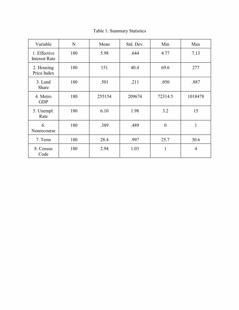
Table 1: Summary Statistics

Variable N Mean Std. Dev. Min Max

1. EffectiveInterest Rate

180 5.98 .644 4.77 7.13

2. HousingPrice Index

180 151 40.4 69.6 277

3. LandShare

180 .501 .211 .050 .887

4. MetroGDP

180 255154 209674 72314.5 1018478

5. Unempl.Rate

180 6.10 1.98 3.2 15

6.Nonrecourse

180 .389 .489 0 1

7. Term 180 28.4 .997 25.7 30.6

8. CensusCode

180 2.94 1.03 1 4

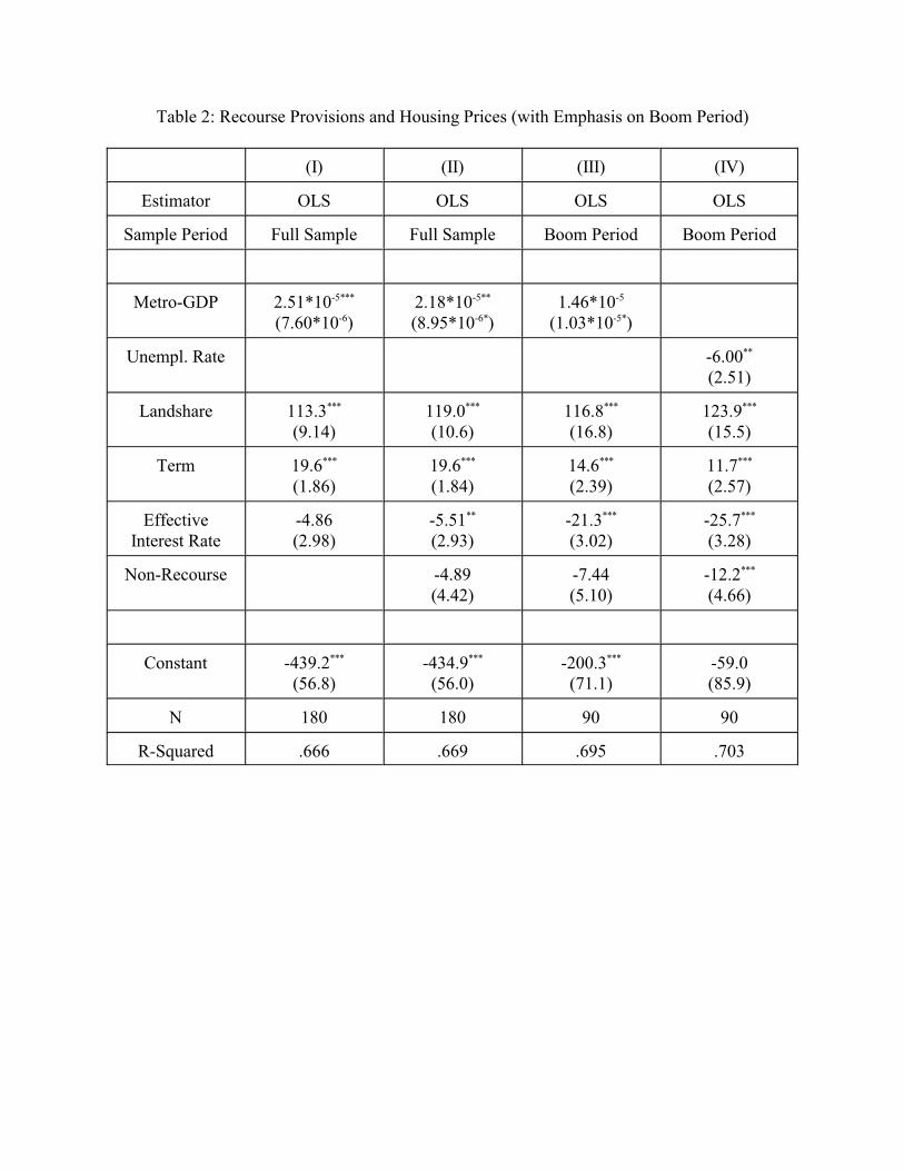
Table 2: Recourse Provisions and Housing Prices (with Emphasis on Boom Period)

(I) (II) (III) (IV)

Estimator OLS OLS OLS OLS

Sample Period Full Sample Full Sample Boom Period Boom Period

Metro-GDP 2.51*10-5***

(7.60*10-6)2.18*10-5**

(8.95*10-6*)1.46*10-5

(1.03*10-5*)

Unempl. Rate -6.00**

(2.51)

Landshare 113.3***

(9.14)119.0***

(10.6)116.8***

(16.8)123.9***

(15.5)

Term 19.6***

(1.86)19.6***

(1.84)14.6***

(2.39)11.7***

(2.57)

EffectiveInterest Rate

-4.86(2.98)

-5.51**

(2.93)-21.3***

(3.02)-25.7***

(3.28)

Non-Recourse -4.89(4.42)

-7.44(5.10)

-12.2***

(4.66)

Constant -439.2***

(56.8)-434.9***

(56.0)-200.3***

(71.1)-59.0(85.9)

N 180 180 90 90

R-Squared .666 .669 .695 .703

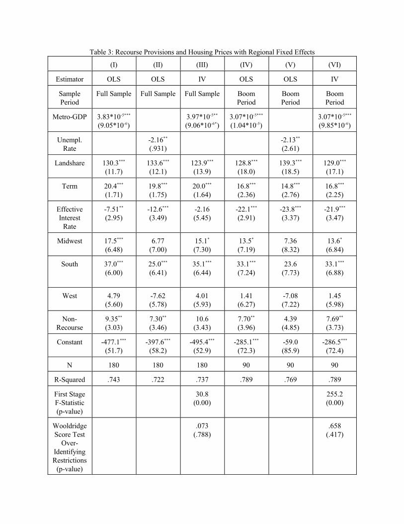
Table 3: Recourse Provisions and Housing Prices with Regional Fixed Effects

(I) (II) (III) (IV) (V) (VI)

Estimator OLS OLS IV OLS OLS IV

SamplePeriod

Full Sample Full Sample Full Sample BoomPeriod

BoomPeriod

BoomPeriod

Metro-GDP 3.83*10-5***

(9.05*10-6)3.97*10-5**

(9.06*10-6*)3.07*10-5***

(1.04*10-5)3.07*10-5***

(9.85*10-6)

Unempl.Rate

-2.16**

(.931)-2.13**

(2.61)

Landshare 130.3***

(11.7)133.6***

(12.1)123.9***

(13.9)128.8***

(18.0)139.3***

(18.5)129.0***

(17.1)

Term 20.4***

(1.71)19.8***

(1.75)20.0***

(1.64)16.8***

(2.36)14.8***

(2.76)16.8***

(2.25)

EffectiveInterest

Rate

-7.51**

(2.95)-12.6***

(3.49)-2.16(5.45)

-22.1***

(2.91)-23.8***

(3.37)-21.9***

(3.47)

Midwest 17.5***

(6.48)6.77

(7.00)15.1*

(7.30)13.5*

(7.19)7.36

(8.32)13.6*

(6.84)

South 37.0***

(6.00)25.0***

(6.41)35.1***

(6.44)33.1***

(7.24)23.6

(7.73)33.1***

(6.88)

West 4.79(5.60)

-7.62(5.78)

4.01(5.93)

1.41(6.27)

-7.08(7.22)

1.45(5.98)

Non-Recourse

9.35**

(3.03)7.30**

(3.46)10.6

(3.43)7.70**

(3.96)4.39

(4.85)7.69**

(3.73)

Constant -477.1***

(51.7)-397.6***

(58.2)-495.4***

(52.9)-285.1***

(72.3)-59.0(85.9)

-286.5***

(72.4)

N 180 180 180 90 90 90

R-Squared .743 .722 .737 .789 .769 .789

First StageF-Statistic(p-value)

30.8(0.00)

255.2(0.00)

WooldridgeScore Test

Over-IdentifyingRestrictions

(p-value)

.073(.788)

.658(.417)

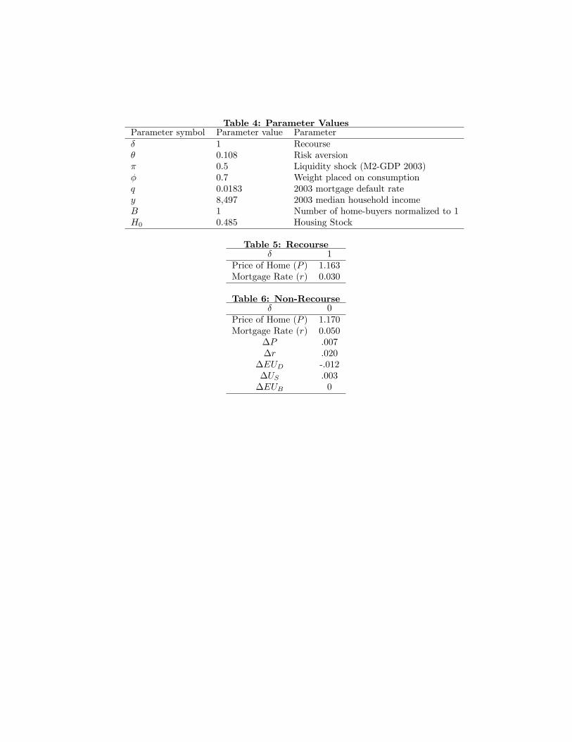
Table 4: Parameter ValuesParameter symbol Parameter value Parameter 1 Recourse 0.108 Risk aversion 0.5 Liquidity shock (M2-GDP 2003) 0.7 Weight placed on consumptionq 0.0183 2003 mortgage default ratey 8,497 2003 median household incomeB 1 Number of home-buyers normalized to 1H0 0.485 Housing Stock

Table 5: Recourse 1

Price of Home (P ) 1.163Mortgage Rate (r) 0.030

Table 6: Non-Recourse 0

Price of Home (P ) 1.170Mortgage Rate (r) 0.050

P .007r .020

EUD -.012US .003EUB 0

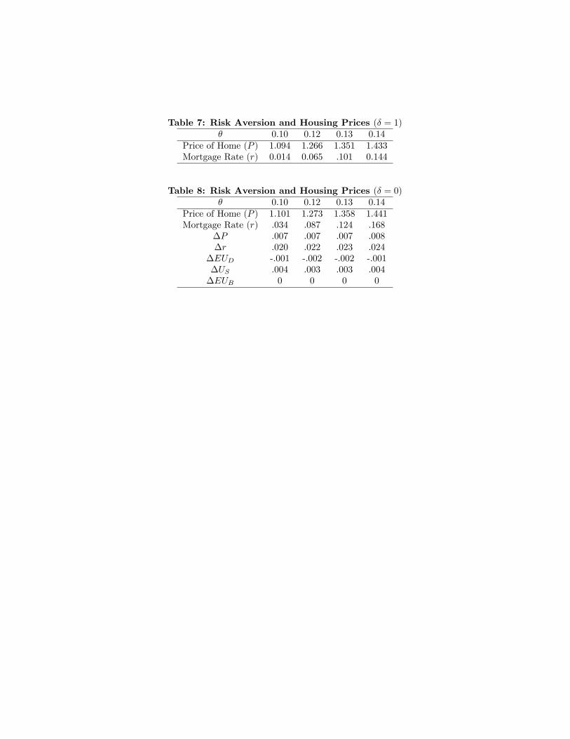
Table 7: Risk Aversion and Housing Prices ( = 1) 0.10 0.12 0.13 0.14

Price of Home (P ) 1.094 1.266 1.351 1.433Mortgage Rate (r) 0.014 0.065 .101 0.144

Table 8: Risk Aversion and Housing Prices ( = 0) 0.10 0.12 0.13 0.14

Price of Home (P ) 1.101 1.273 1.358 1.441Mortgage Rate (r) .034 .087 .124 .168

P .007 .007 .007 .008r .020 .022 .023 .024

EUD -.001 -.002 -.002 -.001US .004 .003 .003 .004EUB 0 0 0 0

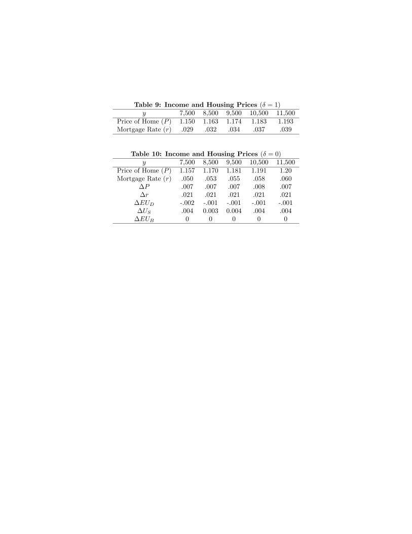
Table 9: Income and Housing Prices ( = 1)y 7,500 8,500 9,500 10,500 11,500

Price of Home (P ) 1.150 1.163 1.174 1.183 1.193Mortgage Rate (r) .029 .032 .034 .037 .039

Table 10: Income and Housing Prices ( = 0)y 7,500 8,500 9,500 10,500 11,500

Price of Home (P ) 1.157 1.170 1.181 1.191 1.20Mortgage Rate (r) .050 .053 .055 .058 .060

P .007 .007 .007 .008 .007r .021 .021 .021 .021 .021

EUD -.002 -.001 -.001 -.001 -.001US .004 0.003 0.004 .004 .004EUB 0 0 0 0 0