workshops on integrating climate change with ...€¦ · web viewthis document is disseminated...
TRANSCRIPT

Federal Highway Administration
Energy and Emissions Reduction Policy Analysis Tool User’s Guide
FHWA-HEPN-10
In Partial Fulfillment of Task 1.0DTFH61-09-F-00117
December 2011
Prepared for
Federal Highway Administration
Prepared byResource Systems Group, Inc.55 Railroad RowWhite River Junction, VT 05001802.295.4999

Notice
This document is disseminated under the sponsorship of the U.S. Department of Transportation in the interest of information exchange. The U.S. Government assumes no liability for use of the information contained in this document. This report does not constitute a standard, specification, or regulation.
The United States Government does not endorse products or manufacturers. Trademarks or manufacturers’ names appear herein only because they are considered essential to the objective of this document.
Quality Assurance Statement
The Federal Highway Administration (FHWA) provides high-quality information to serve Government, industry, and the public in a manner that promotes public understanding. Standards and policies are used to ensure and maximize the quality, objectivity, utility, and integrity of its information. The FHWA periodically reviews quality issues and adjusts its programs and processes to ensure continuous quality improvement.
Acknowledgements
The FHWA acknowledges the development work carried out by the Oregon Department of Transportation’s Transportation Planning Analysis Unit on the GreenSTEP model, on which the FHWA Energy and Emissions Reduction Policy Analysis Tool is based.

FHWA Energy and Emissions Reduction Policy Analysis Tool User’s Guide
EXECUTIVE SUMMARY
The FHWA Energy and Emissions Reduction Policy Analysis Tool (FHWA tool) is a screening tool to compare, contrast, and analyze the effects of various greenhouse gas (GHG) reduction policy scenarios on GHG emissions from the surface transportation sector at a statewide level. The FHWA tool estimates the amount of travel (in terms of vehicle miles traveled) and the resulting GHG emissions, including fuel use (and electricity use for battery charging) by autos, light trucks, transit vehicles, and heavy trucks.
This FHWA Tool User’s Guide steps through the stages of installing, setting up, and running the FHWA tool, as well as analyzing the outputs from scenarios that are tested. The user’s guide is accompanied by the FHWA Tool Model Documentation that describes the model objectives, the model design, the implementation platform, the data sources used for model estimation, and the estimation of each of the model components.
The FHWA tool is a policy analysis tool, and should not be used for specific project or plan evaluation. The FHWA tool complements tools such as EPA’s MOVES (MOtor Vehicle Emission Simulator)1 by providing rapid analysis of many scenarios that combine effects of various policy and transportation system changes. Users wishing to estimate detailed emissions for projects or corridors, or to evaluate detailed regional transportation impacts, should not rely on the FHWA tool. Such users should plan to use a project-level or regional travel demand model in conjunction with MOVES. This user’s guide includes explanations of how to take MOVES inputs and prepare them for use as inputs to the FHWA tool. The user’s guide describes how to develop each FHWA tool input file in turn; if the input can be obtained from MOVES inputs, then this is explained. In addition, the user’s guide summarizes the inputs that can be transferred from MOVES in the final section of the document, which also covers other aspects of integrating the FHWA tool and MOVES in scenario testing work.
The FHWA tool is implemented in the free R data analysis language.2 R provides a powerful, high-performance environment for data analysis that can be used interactively, as well as for scripted programs such as the FHWA tool. All code and data used in the FHWA tool analyses is freely available, and the code and data inputs can be reconfigured by technically adept users should that be necessary to support a specific analysis. The user’s guide provides links to R resources but it is not intended to be a guide to using R.
1 http://www.epa.gov/otaq/models/moves/index.htm2 http://www.r-project.org
Prepared by RSG, December 2011 Page

FHWA Energy and Emissions Reduction Policy Analysis Tool User’s Guide
TABLE OF CONTENTS
1 Introduction............................................................................................................................................................1
1.1 Introduction to the FHWA Tool.....................................................................................................................1
1.2 The FHWA Tool User’s Guide Structure.....................................................................................................1
2 Model Objectives..................................................................................................................................................3
3 Model Design..........................................................................................................................................................4
4 Installing R............................................................................................................................................................12
4.1 What is R?..............................................................................................................................................................12
4.2 Downloading R...................................................................................................................................................12
4.3 Installing R............................................................................................................................................................12
4.4 R Resources..........................................................................................................................................................12
5 Overview of FHWA tool Files........................................................................................................................13
6 Installing and running the FHWA tool......................................................................................................14
6.1 Installing the FHWA tool................................................................................................................................14
6.2 Running the FHWA tool..................................................................................................................................16
7 Developing the input files..............................................................................................................................19
7.1 Model Directory.................................................................................................................................................19
7.2 Scenarios Directory..........................................................................................................................................37
8 Estimation of sub models...............................................................................................................................62
8.1 Sub models...........................................................................................................................................................63
9 Designing scenarios..........................................................................................................................................69
9.1 Instructions for testing a selection of scenarios..................................................................................69
10 Analysis of results............................................................................................................................................. 74
10.1 Organization of outputs..................................................................................................................................74
10.2 Analysis concepts..............................................................................................................................................75
11 Integration with MOVES.................................................................................................................................76
11.1 Using MOVES inputs and parameters in the FHWA tool..................................................................76
11.2 Using the FHWA tool to generate MOVES inputs................................................................................77
11.3 Maintaining consistency between the FHWA tool and MOVES.....................................................78
Prepared by RSG, December 2011 Page

FHWA Energy and Emissions Reduction Policy Analysis Tool User’s Guide
Prepared by RSG, December 2011 Page
FHWA Energy and Emissions Reduction Policy Analysis Tool User’s Guide
LIST OF FIGURESFigure 1: Design of Model for Estimating GHG from Passenger and Truck Travel........................................................5Figure 2: R Shortcut Properties Window....................................................................................................................17Figure 3: Screenshot of R GUI and FHWA tool progress messages for a 2005 run.....................................................18Figure 4: File layout for arterial_lane_miles.csv (complete file shown).....................................................................20Figure 5: File layout for ave_rural_pop_density.csv (partial file shown)....................................................................21Figure 6: File layout for county_groups.csv (partial file shown).................................................................................22Figure 7: File layout for freeway_lane_miles.csv (complete file shown)....................................................................22Figure 8: File layout for global_values.txt..................................................................................................................24Figure 9: File layout for GreenSTEP_$CongModel_ $FwySpdMpgAdj.. (complete table shown)...............................26Figure 10: File layout for GreenSTEP_$HtProb.HtAp (partial file shown)...................................................................27Figure 11: File layout for PersonDf.txt (partial file shown).........................................................................................27Figure 12: File layout for GreenSTEP_$TruckBusAgeDist.AgTy (partial file shown)....................................................28Figure 13: File layout for GreenSTEP_$VehProp_$AgCumProp.AgTy (partial file shown)..........................................30Figure 14: File layout for GreenSTEP_$VehProp_$AgIgProp.AgIgTy (partial file shown)...........................................30Figure 15: File layout for OrVehSmry..RData (partial file shown)...............................................................................30Figure 16: File layout for hh_dvmt_to_road_dvmt.csv (complete file shown)...........................................................31Figure 17: File layout for HsldXXXX.RData (partial file shown)..................................................................................32Figure 18: File layout for mpo_base_dvmt_parm.csv (complete file shown).............................................................33Figure 19: File layout for pop_by_age_XXXX.csv (partial file shown).........................................................................34Figure 20: File layout for transit_revenue_miles.csv (complete file shown)..............................................................34Figure 21: File layout for truck_bus_fc_dvmt_split.csv (complete file shown)..........................................................35Figure 22: File layout for ugb_areas.csv (partial file shown)......................................................................................36Figure 23: File layout for urban_rural_pop_splits.csv (partial file shown).................................................................37Figure 24: File layout for age_adj.csv (complete file shown).....................................................................................39Figure 25: File layout for auto_lighttruck_fuel.csv (complete file shown).................................................................40Figure 26: File layout for auto_lighttruck_mpg.csv (partial file shown).....................................................................41Figure 27: File layout for bus_fuels.csv (partial file shown).......................................................................................42Figure 28: File layout for carshare.csv (partial file shown).........................................................................................42Figure 29: File layout for costs.csv (complete file shown)..........................................................................................43Figure 30: File layout for eco_tire.csv (complete file shown).....................................................................................44Figure 31: File layout for ev_characteristics.csv (partial file shown)..........................................................................45Figure 32: File layout for fuel_co2.csv (complete file shown)....................................................................................46Figure 33: File layout for fwy_art_growth.csv (complete file shown)........................................................................47Figure 34: File layout for heavy_truck_fuel.csv (complete file shown)......................................................................48Figure 35: File layout for hvy_veh_mpg_mpk.csv (partial file shown).......................................................................49Figure 36: File layout for light_vehicles.csv (partial file shown).................................................................................50Figure 37: File layout for lttruck_prop.csv (partial file shown)...................................................................................51Figure 38: File layout for metro_incident_reduction.csv (complete file shown)........................................................51Figure 39: File layout for metropolitan_urban_type_proportions.csv (complete file shown)....................................52Figure 40: File layout for optimize.csv (complete file shown)....................................................................................53Figure 41: File layout for parking.csv (partial file shown)...........................................................................................54
Prepared by RSG, December 2011 Page

FHWA Energy and Emissions Reduction Policy Analysis Tool User’s Guide
Figure 42: File layout for payd.csv (complete file shown)..........................................................................................55Figure 43: File layout for per_cap_inc.csv (complete file shown)..............................................................................56Figure 44: File layout for phev_characteristics.csv (partial file shown)......................................................................57Figure 45: File layout for power_co2.csv (partial file shown).....................................................................................57Figure 46: File layout for regional_inc_prop.csv (complete file shown).....................................................................58Figure 47: File layout for tdm.csv (partial file shown)................................................................................................59Figure 48: File layout for transit_growth.csv (partial file shown)...............................................................................60Figure 49: File layout for ugb_area_growth_rates.csv (partial file shown)................................................................61Figure 50: File layout for urban_rural_growth_splits.csv (partial file shown)............................................................61
Prepared by RSG, December 2011 Page

FHWA Energy and Emissions Reduction Policy Analysis Tool User’s Guide
1 INTRODUCTION
1.1 Introduction to the FHWA Tool
The FHWA Energy and Emissions Reduction Policy Analysis Tool (the FHWA tool) is a screening tool to compare, contrast, and analyze the effects of various GHG reduction policy scenarios on GHG emissions from the surface transportation sector at a statewide level. The FHWA tool estimates the amount of travel (in terms of vehicle miles traveled) and the resulting GHG emissions, including fuel use (and electricity use for battery charging) by autos, light trucks, transit vehicles, and heavy trucks.
Note: The FHWA tool is a policy analysis tool, and should not be used for specific project or plan evaluation. The FHWA tool complements tools such as EPA’s MOVES (MOtor Vehicle Emission Simulator)3 by providing rapid analysis of many scenarios that combine effects of various policy and transportation system changes. In order to provide quick response comparing many scenarios, the FHWA tool makes a number of simplifying assumptions (consistent with MOVES and with advanced regional travel demand modeling practice) that limit the detail and precision of its outputs. Users wishing to estimate detailed emissions for projects or corridors, or to evaluate detailed regional transportation impacts, should not rely on the FHWA tool. Such users should plan to use a project-level or regional travel demand model in conjunction with MOVES. To ensure that policy testing performed with the FHWA tool produces results that are consistent with more detailed analysis carried out using MOVES, users should use MOVES inputs in the FHWA tool; this process is described in the user’s guide.
The FHWA tool is implemented in the free R data analysis language.4 R provides a powerful, high-performance environment for data analysis that can be used interactively as well as for scripted programs such as the FHWA tool. All code and data used in the FHWA tool analyses is freely available, and the code and data inputs can be reconfigured by technically adept users should that be necessary to support a specific analysis.
1.2 The FHWA Tool User’s Guide Structure
This FHWA Tool User’s Guide will step you through the stages of installing, setting up, and running the FHWA tool, as well as analyzing the outputs from scenarios that you decide to test. The guide is divided into eleven sections:
1. Introduction: Intended use of the FHWA tool
2. Model Objectives
3. Model Design
4. Installing R
5. Overview of FHWA tool files
6. Installing and running the FHWA tool
3 http://www.epa.gov/otaq/models/moves/index.htm4 http://www.r-project.org
Prepared by RSG, December 2011 Page

FHWA Energy and Emissions Reduction Policy Analysis Tool User’s Guide
7. Developing the input files
8. Estimation of sub models
9. Designing scenarios
10. Analysis of results
11. Integration with MOVES.
Prepared by RSG, December 2011 Page

FHWA Energy and Emissions Reduction Policy Analysis Tool User’s Guide
2 MODEL OBJECTIVES
The FHWA tool is based on the Oregon Department of Transportation (ODOT) Transportation Planning Analysis Unit’s (TPAU’s) “GreenSTEP,” a modeling tool to assess the effects of a large variety of policies and other factors on transportation sector GHG emissions. The FHWA tool was developed to address the following factors, among others:
Changes in population demographics (age structure);
Changes in personal income;
Relative amounts of development occurring in metropolitan, urban, and rural areas;
Metropolitan, other urban, and rural area densities;
Urban form in metropolitan areas (proportion of population living in mixed-use areas with a well interconnected street and walkway system);
Amounts of metropolitan area transit service;
Metropolitan freeway and arterial supplies;
Auto and light truck proportions by year;
Average vehicle fuel economy by vehicle type and year;
Vehicle age distribution by vehicle type;
Electric vehicles (EVs), plug-in hybrid electric vehicles (PHEVs);
Non-motorized vehicles or two-wheeled electric vehicles, such as bicycles, electric bicycles, electric scooters, etc.;
Pricing – fuel, vehicle miles traveled (VMT), parking;
Demand management – employer-based and individual marketing programs;
Car-sharing;
Effects of congestion on fuel economy;
Effects of highway incident management on fuel economy;
Vehicle operation and maintenance – eco-driving, low rolling resistance tires, speed limits;
Carbon intensity of fuels; and
Carbon production from the electric power that is generated to run electric vehicles.
The FHWA tool addresses an entire State on a county basis in order to be responsive to regional differences. It distinguishes between households living in metropolitan, other urban, and rural areas to reflect the different characteristics of those areas in terms of density, urban form, transportation system characteristics, and transportation demand management (TDM) programs.
Prepared by RSG, December 2011 Page

FHWA Energy and Emissions Reduction Policy Analysis Tool User’s Guide
3 MODEL DESIGN
The FHWA tool is a system of disaggregate household-level models; the disaggregate nature of the models is intended to create a behaviorally consistent model. While the FHWA tool began as a sketch-planning model, the level of detail inherent in the current version has moved the FHWA tool out of that realm. Most of the FHWA tool operates at an individual household level where each household that the model synthesizes has individual attributes and where vehicle ownership and use is predicted on an individual synthesized household basis.
An advantage of this approach over a sketch-planning approach is that it better accounts for interactions between policies. For example, a policy that increases urban area density decreases household daily vehicle miles traveled (DVMT) by increasing shortened trips and increasing non-auto travel. Higher densities also increase the market for car-sharing. Increased car-sharing in turn reduces household vehicle ownership, which also reduces household DVMT. Reducing household DVMT also increases the likelihood that a household vehicle could be replaced by an EV and/or increases the proportion of household PHEV mileage that can be traveled on an electric charge. Another benefit of the disaggregate approach is that it provides a means for accounting for the effects of changes in fuel prices and a number of other costs of household travel in a consistent manner. Because household fuel costs are a function of household vehicle fuel economy, in addition to fuel prices, the model accounts for increases in travel that would occur with gains in fuel economy (rebound effect). Finally, modeling at the individual household level allows for better analysis of how different households would be affected by policies in a number of ways.
The FHWA tool is designed to run at a county level. This design concept was motivated by the availability of long-range population projections by age at the county level and the need for the model to be sensitive to regional differences.
Figure 1 shows an overview of the FHWA tool model design (in two parts). The gray boxes in the middle of the figure identify the major steps in the model execution. The number in the lower right-hand corner of each box corresponds to paragraph numbering in the description that follows. The blue boxes on the left side of the figure show the input assumptions on which the calculations are based and which may be altered to represent different policies. The green boxes on the right side of the figure identify the models and methodologies that are used in the calculations. These models and how they were estimated and calibrated are explained in the FHWA Tool Model Documentation.
Prepared by RSG, December 2011 Page

FHWA Energy and Emissions Reduction Policy Analysis Tool User’s Guide
Figure 1: Design of Model for Estimating GHG from Passenger and Truck Travel
Prepared by RSG, December 2011 Page

FHWA Energy and Emissions Reduction Policy Analysis Tool User’s Guide
Figure 1: Design of Model for Estimating GHG from Passenger and Truck Travel (continued)
Prepared by RSG, December 2011 Page

FHWA Energy and Emissions Reduction Policy Analysis Tool User’s Guide
The following is an explanation of major steps in the model execution shown in the gray boxes in Figure 1.
1. Create Synthetic Households: A set of households is created for each forecast year that represents the likely household composition for each county, given the county-level forecast of persons by age. Each household is described in terms of the number of persons in each of six age categories residing in the household. A total household income is assigned to each household, given the ages of persons in the household and the average per capita income of the region where the household resides.
2. Calculate Population Densities and Other Land Use Characteristics: Population density and land use characteristics are important variables in the vehicle ownership, vehicle travel, and vehicle type models. Models were developed to estimate density and land use characteristics at a Census tract level based on more aggregate policy assumptions about metropolitan and other urban area characteristics.5 Each household is assigned to a metropolitan, other urban, or rural development type in the county where it is located based on policy assumptions about the proportions of population growth that will occur in each type. The overall densities for metropolitan and other urban areas in each county are calculated based on policy assumptions for urban growth boundary expansions. Households assigned to metropolitan areas are assigned to population density drawn from a likely household density distribution corresponding to the overall metropolitan area density. Households assigned to other urban areas are assigned the overall population density for non-metropolitan areas in the county. Households assigned to rural areas are assigned a population density reflecting the predominant rural population density of the county where they are located. Households in urban areas are also assigned to an urban mixed-use setting or not, based on a model using population density. This can be overridden to simulate greater amounts of urban mixed-use development.
3. Calculate Freeway, Arterial, and Public Transit Supply Levels: The number of lane miles of freeways and arterials is computed for each metropolitan area based on base-year inventories and policy inputs as to how rapidly lane miles are added relative to the addition of metropolitan population. For example, a value of one for freeways means that freeway lane miles grow at the same rate as population grows. If population doubles, freeway lane miles would double as well. For public transit, the inputs specify the growth in transit revenue miles relative to the base year. Inputs for each metropolitan area also specify the revenue mile split between electrified rail and buses.
4. Determine Households Affected by Travel Demand Management and/or Vehicle Operations and Maintenance Programs: Each household is assigned as being a participant or not in a number of travel demand management programs (e.g. employee commute options programs, individualized marketing) and/or to vehicle operations and maintenance programs (e.g. eco-driving, low rolling resistance tires) based on policy assumptions about the degree of deployment of those programs and the household characteristics.
5. Calculate Vehicle Ownership and Adjust for Car-sharing: Each household is assigned the number of vehicles it is likely to own based on the number of persons of driving age in the household, whether only elderly persons live in the household, the income of the household, and the population density where the household lives. For metropolitan households, vehicle ownership depends on the freeway supply, transit supply, and whether the household is located in an urban mixed-use area. Households are identified as car-sharing participants or not based on household characteristics and policy assumptions about the deployment of
5 The FHWA tool could be modified to operate at a metropolitan level with data being input for each Census tract.
Prepared by RSG, December 2011 Page

FHWA Energy and Emissions Reduction Policy Analysis Tool User’s Guide
car-sharing. The number of vehicles owned by car-share households is reduced based on a simple model.
6. Calculate Initial Household Daily Vehicle Miles Traveled (DVMT): The average DVMT for each household is modeled based on household information determined in previous steps. There are different models for households residing inside and outside metropolitan (urbanized) areas. The metropolitan model is sensitive to household income, population density of the neighborhood where the household resides, number of household vehicles, whether the household owns no vehicles, the levels of public transportation and freeway supplies in the metropolitan area, the driving-age population in the household, the presence of persons over age 65, and whether the neighborhood is characterized by mixed-use development. The non-metropolitan model is similar but does not include the transit supply, freeway supply, or mixed-use variables.
7. Calculate Non-Price TDM and Non-Motorized Vehicle Adjustment Factors and Adjust Household DVMT: Non-price TDM policies are grouped into two categories, workplace-oriented commute options programs and household-oriented individualized marketing programs. Household DVMT adjustment factors are calculated based on participation in these programs (determined in step #4) and assumptions regarding the average reductions in household DVMT that the programs produce. Adjustment factors are also calculated to account for the potential substitution of non-motorized vehicles travel for household DVMT. For the purposes of the FHWA tool, non-motorized vehicles are bicycles, electric bicycles, and similar vehicles. The model predicts the potential amount of household DVMT that could be diverted to non-motorized vehicle travel using a model of the amount of household vehicle travel occurring in single-occupant vehicle (SOV) tours of less than various specified lengths. This model is sensitive to household income, population density, household size, urban mixed-use character, and average household DVMT. The amount of diversion is a function of this potential, assumptions about non-motorized vehicle ownership rates, and assumptions about the proportion of the potential diverted vehicle travel that may be suitable for non-motorized vehicle travel. After the TDM and non-motorized factors have been calculated, they are applied to the initial household DVMT estimates to produce adjusted estimates.
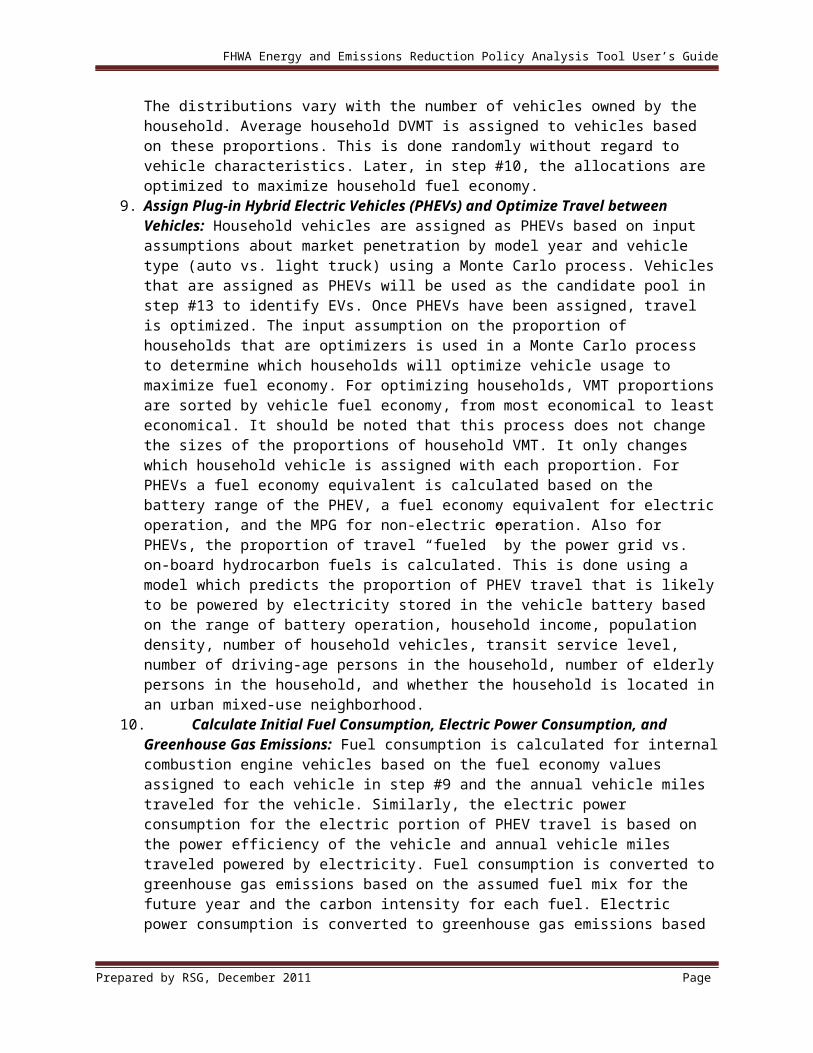
8. Calculate Vehicle Types, Ages, Initial Fuel Economy, and Assign DVMT to Vehicles: Two body styles of household vehicles are considered – automobiles and light trucks. The latter includes pickup trucks, sport-utility vehicles, and vans. A model predicts the probability that a household vehicle is a light truck based on the number of vehicles in the household, the household income, the population density where the household resides, and whether the household lives in an urban mixed-use area. This probability is then used as a sampling probability to determine stochastically whether each household vehicle is an automobile or light truck. Once the type of vehicle has been assigned to each vehicle, the age of each vehicle is determined. This is done by sampling from vehicle age distributions by vehicle type and household income group. These distributions may be changed based on input assumptions about changes in fleet turnover rates. Once vehicle ages have been determined, initial assignments of vehicle fuel economy are made based on input assumptions about average vehicle fuel economy by model year and vehicle type. Fuel economy is adjusted in later steps for vehicles identified as plug-in hybrid electric vehicles (PHEVs) and electric vehicles (EVs) and to reflect the effects of congestion and vehicle operation and maintenance on fuel economy. Vehicles are assigned a proportion of the estimated household DVMT based on distributions of how annual household mileage is allocated among multiple vehicles. The distributions vary with the number of vehicles owned by the household. Average household DVMT is assigned to vehicles based on these proportions.
Prepared by RSG, December 2011 Page

FHWA Energy and Emissions Reduction Policy Analysis Tool User’s Guide
This is done randomly without regard to vehicle characteristics. Later, in step #10, the allocations are optimized to maximize household fuel economy.
9. Assign Plug-in Hybrid Electric Vehicles (PHEVs) and Optimize Travel between Vehicles: Household vehicles are assigned as PHEVs based on input assumptions about market penetration by model year and vehicle type (auto vs. light truck) using a Monte Carlo process. Vehicles that are assigned as PHEVs will be used as the candidate pool in step #13 to identify EVs. Once PHEVs have been assigned, travel is optimized. The input assumption on the proportion of households that are optimizers is used in a Monte Carlo process to determine which households will optimize vehicle usage to maximize fuel economy. For optimizing households, VMT proportions are sorted by vehicle fuel economy, from most economical to least economical. It should be noted that this process does not change the sizes of the proportions of household VMT. It only changes which household vehicle is assigned with each proportion. For PHEVs a fuel economy equivalent is calculated based on the battery range of the PHEV, a fuel economy equivalent for electric operation, and the MPG for non-electric operation. Also for PHEVs, the proportion of travel “fueled” by the power grid vs. on-board hydrocarbon fuels is calculated. This is done using a model which predicts the proportion of PHEV travel that is likely to be powered by electricity stored in the vehicle battery based on the range of battery operation, household income, population density, number of household vehicles, transit service level, number of driving-age persons in the household, number of elderly persons in the household, and whether the household is located in an urban mixed-use neighborhood.
10. Calculate Initial Fuel Consumption, Electric Power Consumption, and Greenhouse Gas Emissions: Fuel consumption is calculated for internal combustion engine vehicles based on the fuel economy values assigned to each vehicle in step #9 and the annual vehicle miles traveled for the vehicle. Similarly, the electric power consumption for the electric portion of PHEV travel is based on the power efficiency of the vehicle and annual vehicle miles traveled powered by electricity. Fuel consumption is converted to greenhouse gas emissions based on the assumed fuel mix for the future year and the carbon intensity for each fuel. Electric power consumption is converted to greenhouse gas emissions based on the amount of electric power consumed and the assumed rates of greenhouse gas emissions per unit of power consumed.
11. Calculate Household Mileage Costs: Total variable vehicle costs (costs that vary based on vehicle usage) are calculated for each household. These costs include the cost of fuels and electric power. They may also include, depending on policy assumptions, carbon taxes, VMT taxes, pay-as-you-drive (PAYD) insurance rates, and parking charges. For metropolitan areas, a model is applied to determine how many working-age persons in each household pay for parking at their worksite, based on input assumptions about the proportion of employees in the metropolitan area with employers who charge for parking or who must pay for parking at commercial lots, and how easily the parking charges may be avoided by parking for free on the street or at free parking lots. The model also estimates the proportion of non-work household trips and another model calculates daily parking charges for households paying for employment parking and other trip parking.
12. Recalculate Household DVMT and Reallocate to Vehicles: A household budget model is used to adjust household DVMT to reflect the effect of variable vehicle costs on the amount of household travel. The adjusted household DVMT is allocated to vehicles in proportion to the previous allocation. The travel reduction proportions from TDM and non-motorized vehicle use calculated in step #7 are applied.
13. Assign Electric Vehicles (EVs) and Calculate Adjustments to Fuel and Electric Power Consumption: Household vehicles are identified as candidates to be electric vehicles based on how their vehicle usage patterns compare with the average travel range of EVs for their
Prepared by RSG, December 2011 Page

FHWA Energy and Emissions Reduction Policy Analysis Tool User’s Guide
vehicle model years. A vehicle is considered to be a candidate to be an EV only if the vehicle was identified as a PHEV in step #9 and if the EV range is large enough to accommodate most of the expected usage of the vehicle by the household. To determine this, the 95th percentile DVMT is determined for each vehicle as a function of the average DVMT of the vehicle. Candidate vehicles are then identified as EVs based on input assumptions regarding the market penetration of EVs among candidate vehicles. EVs are selected only from the pool of vehicles previously identified as PHEV so that the cost calculations in step #11 would be close to representing EV costs.
14. Calculate Auto and Light Truck Travel on Metropolitan Area Roadways: Since roadway congestion affects vehicle speeds and fuel economy, it is necessary to calculate roadway VMT in metropolitan areas. This is done by applying a factor calculated for the base year (2005) that is the ratio of urbanized area road auto and light truck DVMT calculated from Highway Performance Monitoring System (HPMS) data and the estimate of household DVMT of urbanized area households calculated by the FHWA tool. This ratio is calculated for each metropolitan area.
15. Calculate Truck and Bus DVMT and Assign Proportions to Metropolitan Areas: Statewide truck VMT is calculated based on changes in the total state income. As a default, a one-to-one relationship between state income growth and truck VMT growth is assumed. In other words, a doubling of total state income would result in a doubling of truck VMT. Portions of the statewide truck DVMT are assigned to metropolitan areas based on estimates derived from HPMS data. Bus DVMT is calculated from bus revenue miles that are factored up to total vehicle miles to account for miles driven in non-revenue service.
16. Adjust Metropolitan Area Fuel Economy to Account for Congestion: Auto and light truck DVMT, truck DVMT and bus DVMT in metropolitan areas are allocated to freeways, arterials, and other roadways. Truck and bus DVMT are allocated based on mode-specific data derived from the HPMS data. Auto and light truck DVMT are allocated based on a combination of HPMS-derived factors and a model that is sensitive to the relative supplies of freeway and arterial lane miles. System-wide ratios of DVMT to lane miles for freeways and arterials are used to allocate DVMT to congestion levels using congestion levels defined by the Texas Transportation Institute for the Urban Mobility Report. Each freeway and arterial congestion level is associated with an average trip speed for conditions that do and do not include highway incidents. Overall average speeds by congestion level are calculated based on input assumptions about the degree of incident management. Speed vs. fuel efficiency relationships for light vehicles, trucks, and buses are used to adjust the fleet fuel efficiency averages computed for each metropolitan area.
17. Adjust Fuel Economy to Account for Eco-Driving and Low Rolling Resistance Tires: The average fuel economy of households identified as eco-drivers is adjusted based on assumed adjustment rates. Adjustment to fuel economy and power consumption is also made for households identified as having low rolling resistance tires on their vehicles.
18. Calculate Final Household Light Vehicle Fuel Consumption, Electric Power Consumption, Greenhouse Gas Emissions and Costs: Fuel consumption, electric power consumption, and greenhouse gas emissions are recalculated to reflect the adjusted fuel economy and power consumption.
19. Calculate Bus, Truck, and Passenger Rail Fuel Consumption and Greenhouse Gas Emissions Adjusted for Congestion: The age distributions of trucks and buses are computed from base year distributions and input assumptions about changes in fleet turnover. The average MPG of the specific fleets is computed from the respective age distributions and respective assumptions about future MPG by model year. These fuel economy values are adjusted for the truck and bus VMT in metropolitan areas using the adjustment factors computed in step #16.
Prepared by RSG, December 2011 Page

FHWA Energy and Emissions Reduction Policy Analysis Tool User’s Guide
Prepared by RSG, December 2011 Page

FHWA Energy and Emissions Reduction Policy Analysis Tool User’s Guide
4 INSTALLING R
4.1 What is R?
The FHWA tool is implemented in R. R is a freely available language and environment for statistical computing and graphics which provides a wide variety of statistical and graphical techniques: linear and nonlinear modeling, statistical tests, time series analysis, classification, clustering, etc. R is available from the Comprehensive R Archive Network (CRAN), a network of ftp and web servers around the world that store identical up-to-date versions of code and documentation for R.
4.2 Downloading R
Download the latest version of R from CRAN: http://cran.r-project.org/. R is available for Linux, Mac OS X, and Windows; the current version (as of December 2011) is R-2.14.0.
4.3 Installing R
Installation instructions are at http://cran.r-project.org/doc/FAQ/R-FAQ.html#How-can-R-be-installed_003f. There are two platform specific FAQ sites that contain detailed installation instructions for Windows (http://cran.r-project.org/bin/windows/base/rw-FAQ.html) and Mac OS X (http://cran.r-project.org/bin/macosx/RMacOSX-FAQ.html).
4.4 R Resources
There are many resources for helping newer R users become more familiar with using R for data analysis and modeling. Here are some places to get started:
Manual and introduction to R: http://cran.r-project.org/manuals.html Journal: The R Journal (http://journal.r-project.org/) is the refereed journal of the R project
for statistical computing. It features short to medium length articles covering topics that might be of interest to users or developers of R.
Wiki: http://rwiki.sciviews.org/doku.php Online resource list: http://rwiki.sciviews.org/doku.php?id=links:links Books: http://www.r-project.org/doc/bib/R-books.html R function reference card: http://cran.r-project.org/doc/contrib/Short-refcard.pdf R search engine: http://www.rseek.org/ Webinar: FHWA’s TMIP Webinar series included a webinar on travel modeling using R in
February 2011 (http://tmip.fhwa.dot.gov/webinars/usingR)
Prepared by RSG, December 2011 Page

FHWA Energy and Emissions Reduction Policy Analysis Tool User’s Guide
5 OVERVIEW OF FHWA TOOL FILES
The FHWA tool and its documentation are available for download as files from the FHWA tool website (http://www.planning.dot.gov/FHWA_tool/default.asp):
1. User’s Guide: EERPAT_Users_Guide_21.pdf, the present document, steps through the stages of installing, setting up, and running the FHWA tool, as well as analyzing the outputs from scenarios.
2. Documentation: EERPAT_Model_Documentation_21.pdf. This is a thorough introduction to the FHWA tool and its sub models, including details of the estimation of the sub models. This covers in detail the technical aspects of the FHWA tool’s model structure and the sub models that are only briefly introduced in this user’s guide.
3. EERPAT_21.zip: a zip file containing the FHWA tool application (version 2.1), and a blank set of input files. The zip file includes all of the files required to set up and run the model, but data must be added before the model can be run. It extracts with the directory structure required to run the model.
4. EERPAT_Florida_21.zip: a zip file containing the FHWA tool application, with example input files for Florida. The zip file includes all of the files required to set up and run the Florida implementation of the model. It extracts with the directory structure required to run the model.
5. EERPAT_Estimation_21.zip: this contains the input data and scripts that were used to estimate each of the sub models. Re-estimation of some of the sub models using local data is discussed later in this user’s guide.
Prepared by RSG, December 2011 Page
FHWA Energy and Emissions Reduction Policy Analysis Tool User’s Guide
6 INSTALLING AND RUNNING THE FHWA TOOL
6.1 Installing the FHWA tool
The zip files “EERPAT_21.zip” and “EERPAT_Florida_21.zip”, which are available for download from the FHWA tool website, each contain the FHWA tool application. The FHWA tool is not pre-populated with “default” inputs in the way that MOVES and some other models are. The example model is supplied with a complete set of input files for Florida (developed as part of FHWA’s review and dissemination of the FHWA tool). These are example inputs and are not intended to serve as a fully validated set of inputs for other areas.
Once a zip file is downloaded to your computer, install it by using a zip file utility to extract the files to a directory on your computer, e.g. C:\FHWATool\. The files will extract into the directory structure required to run the model:
ModelPop_forecasts
Scenariosbase
inputsoutputs
futureinputsoutputs
ScriptsAnalysis Setup
In order to maintain the Florida example for reference and to have one installation where you can add new input files for the application of the FHWA tool in your state, you will need to install the model twice times, each time unzipping one of the two zip files into a separate directory.
6.1.1 Model DirectoryThis directory contains all of the model input files that make up the FHWA tool model. These files are described below in Section 7 “Developing the Input Files.” Once the model has been set up, the files in this directory are typically held constant across scenarios.
6.1.2 Scenarios DirectoryThis directory contains the inputs and outputs of all the policy scenarios that are modeled. There is one folder per scenario. The “base” directory contains the base scenario information. The base scenario is the model run for current conditions and policies, i.e. the scenario against which alternative scenarios can be compared. The “run_parameters.txt” file is set up with the expectation that the directory is called “base.” If the base scenario directory is to be named something else, then the “BaseScenName” parameter in the “run_parameters.txt” file should be edited by the analyst to
Prepared by RSG, December 2011 Page

FHWA Energy and Emissions Reduction Policy Analysis Tool User’s Guide
identify the directory name that is used. The analyst must run the base scenario for at least the base year (which is set at 2005) before running any future scenarios.
There may be one or more future scenarios. There are no caveats for naming the future scenario directories. Each scenario directory includes two subdirectories: inputs and outputs. The inputs directory includes all of the input files needed to specify a scenario. The outputs directory contains all of the output files that are produced by the model. The FHWA tool creates an output directory during the run.
The input files in the base/inputs/ and future/inputs/ directories are described below in Section 7 “Developing the Input Files.”
The outputs directory for each scenario contains all of the files saved by the FHWA tool in the course of a model run. The outputs directory contains a directory for each forecast year for which the model was run (the analyst can choose to run any year between 1990 and 2050 in 5-year increments). In each forecast year directory there are files containing the household simulation results for each county. The file names are built from the name of the county and a “.RData” extension. There is also a set of files that contains data at a more aggregate level. Most of the files are tabulations by metropolitan area for calculations that take place at that level of detail. The “Year2005” directory also contains a file named “Pop.CoDt.RData” which is a tabulation of base year population by county and development type. The outputs are discussed below in Section 10 “Analysis of Results.”
6.1.3 Scripts DirectoryThis directory contains all of the R scripts that run portions of the FHWA tool. They are as follows:
GreenSTEP.r – This is the main script which runs the FHWA tool. It calls all of the other scripts as needed.
GreenSTEP_Hh_Synthesis.r – This script generates a complete list of households, each described in terms of the number of household members in each of six age categories, for each county and forecast year from population age cohort forecasts by county and year.
GreenSTEP_Inputs.r – This script reads in all the model input files and scenario input files used in the FHWA tool.
GreenSTEP_Sim.r – This script performs all of the household level simulations to predict vehicle ownership, vehicle travel, and vehicle types.
license.txt – This text file contains the software license for the FHWA tool. The FHWA tool is open-source software that is copyrighted by the Oregon Department of Transportation and licensed under the terms of the GNU General Public License Version 3.
6.1.4 Analysis DirectoryThis directory contains R scripts that load and analyze scenario results. It also contains the results of any analysis performed using the scripts. Note that this directory is not currently used but will be used for scripts that help users aggregate, analyze, chart, and map the data.
6.1.5 Setup Directory
Prepared by RSG, December 2011 Page

FHWA Energy and Emissions Reduction Policy Analysis Tool User’s Guide
This directory contains R scripts and datasets to assist with setting up a new application of the FHWA tool. Note that this directory is not currently used but will be used for data and scripts to assist with model setup.
6.2 Running the FHWA tool
The FHWA tool with Florida input files can be immediately run as described in this section of the user’s guide. Once input files have been developed for the application of the FHWA tool in a new State, the same steps will be used to run the FHWA tool. We recommend that the FHWA tool first be run with the provided Florida input files to check that the installation of R is correct and that all of the files have been successfully unzipped and installed.
Shortcuts
Check that the R shortcuts in both the “base” directory and the “future” directory point to the version of R that is currently installed and that “Start in” properties for both shortcuts are set correctly.
1. The shortcut file is “R 2.11.1” and points to the Rgui executable. It is named R 2.11.1 because this was the latest version of R when the FHWA tool was released. However, it should point to whatever version of R is currently installed, for example R 2.14.0 is the latest version of R as of December 2011.
2. Creating a shortcut to R can be done by copying and pasting as a shortcut the Rgui.exe icon located in the bin subdirectory of the relevant R program directory (e.g. C:\Program Files\R\R-2.11.1\bin\Rgui.exe).
3. The properties of the shortcut should be edited so that R will start in the directory for the scenario. If that is not done, R will not know where to find the required files. This can be done by right-clicking on the shortcut and choosing “Properties” in the pop-up menu. The window shown in Figure 2 will appear. Remove anything listed in the “Start in” field and then click on the “OK” button. This will change the shortcut so that it will point R to the directory where the shortcut is located.
Prepared by RSG, December 2011 Page

FHWA Energy and Emissions Reduction Policy Analysis Tool User’s Guide
Figure 2: R Shortcut Properties Window
Run the base scenario
1. Start the R console with the R shortcut in the base directory.
2. Click on the “Buffered output” menu item in the “Misc” menu in the R console so that you can see progress messages in the console. The model will run fine without doing this, but you will not be able to see progress messages as the model runs.
3. Drag and drop the “run_GreenSTEP.r” script from the base directory onto the R console window. This will run the FHWA tool. Figure 3 shows the R GUI and the FHWA tool progress messages at the end of a 2005 run (in this case, just a single year was run).
4. Close the R console window after the model run is completed.
Prepared by RSG, December 2011 Page

FHWA Energy and Emissions Reduction Policy Analysis Tool User’s Guide
Figure 3: Screenshot of R GUI and FHWA tool progress messages for a 2005 run
Run a future scenario
Future scenarios are run in a similar way to the base scenario.
1. Copy the “future” directory and rename as desired, e.g. “future_scenario1”.
2. Since future scenarios are meant to model the effects of different prospective policies, the input files will need to be modified to reflect those policies. The “Designing Scenarios” section of this report discusses setting up alternative future scenarios.
3. Start the R console with the R shortcut in the future scenario directory that you created.
4. Drag and drop the “run_GreenSTEP.r” script from the future scenario directory that you created onto the R console window. This will run the FHWA tool.
5. Close the R console window after the model run is completed.
Prepared by RSG, December 2011 Page

FHWA Energy and Emissions Reduction Policy Analysis Tool User’s Guide
7 DEVELOPING THE INPUT FILES
This section of the user’s guide provides details of the format and role of each of the files in the model directory and the input directories within the base and future scenario folders. Approaches that the analyst can follow to develop or obtain the data in each file are discussed, including how the analyst can create several of the input data files from MOVES inputs if those are available. Examples of each of the files are included in the Florida example model. Each of the files must be present in their respective directories for a model run to be successful (except for files that are indicated as being created during a run). This section does not contain specific recommendations or guidance on the reasonableness of input values; the analyst needs to consider what variation in inputs is reasonable. The analyst should consult other sources of information (some of which are referenced in the FHWA Tool Model Documentation) for what assumptions could be viable.
7.1 Model Directory
Most of the files in the model directory will need to be created by the analyst for the geography in which the FHWA tool is being applied. The corresponding files supplied with the Florida model can be used as templates. After the initial set up, these files are generally not changed again unless model components are re-estimated or base year data are changed. As noted in the description of each file, several of these files are automatically created from other input files during model runs and do not have to be constructed directly by the analyst.
The files in the directory are listed below; descriptions of what they contain and discussion of how to create the data for a new geography follow. File names having a “csv” extension are tabular text files formatted using the comma separated values convention. The “csv” files should include a header line as their first line, as shown in the sample data figures below. File names having an “RData” extension are R binary files. File names having a “txt” extension are text files in a format described for the file.
arterial_lane_miles.csv – base year arterial lane miles by metropolitan area ave_rural_pop_density.csv – base year rural population density by county county_groups.csv – association of counties with regions and metropolitan areas freeway_lane_miles.csv – base year freeway lane miles by metropolitan area global_values.txt – a text file that contains global run parameters GreenSTEP_.RData – R binary object containing all of the estimated models applied by the
FHWA tool and several input data tabulations that are used by the model. hh_dvmt_to_road_dvmt.csv – factors to convert household daily VMT to light vehicle road
daily VMT HsldXXXX.RData – R binary objects that contain the household level population forecasts LtVehDvmtFactor.Ma.RData – R binary object, replaces hh_dvmt_to_road_dvmt.csv when the
model is run mpo_base_dvmt_parm.csv - additional data to calculate metropolitan daily VMT pop_forecasts/pop_by_age_XXXX.csv – population estimates/forecasts by county and age
cohort
Prepared by RSG, December 2011 Page

FHWA Energy and Emissions Reduction Policy Analysis Tool User’s Guide
transit_revenue_miles.csv – annual bus and rail revenue miles per capita by metropolitan area
truck_bus_fc_dvmt_split.csv – proportions of truck and bus daily VMT by functional class ugb_areas.csv – geographic areas within urban growth boundaries urban_rural_pop_splits.csv – proportions of population in each area type by county
7.1.1 arterial_lane_miles.csvFormat: arterial_lane_miles.csv is a table of base year (2005) arterial lane miles by metropolitan area. Figure 4 shows the file layout, with one row per metropolitan area and the values in units of miles.
Use: The arterial lane miles data are used to describe the supply of arterial capacity in the models and calculations that adjust metropolitan area fuel economy to account for congestion.
Source: This file is user created. The analyst can obtain these data from FHWA’s Highway Statistics data (http://www.fhwa.dot.gov/policy/ohim/hs05/roadway_extent.htm) and State DOT data.
Figure 4: File layout for arterial_lane_miles.csv (complete file shown)Msa ArtlnmiMetro 1995EugeneSpringfield 419SalemKeizer 419RogueValley 354Bend 164Corvallis 146
7.1.2 ave_rural_pop_density.csvFormat: ave_rural_pop_density.csv is a table of base year (2005) rural population density by county. Figure 5 shows the file layout, with one row per county and the values in units of people per square mile.
Use: This file is used in the models of household vehicle ownership and vehicle travel.
Source: This file is user created. The analyst can develop this file using Census 2000 block group data (http://www.census.gov/main/www/cen2000.html), more recent population data to update 2000 data to 2005 data (such as county level and incorporated place population estimates from the Census bureau, http://www.census.gov/popest/estbygeo.html, or State sources of land use data), and State-specific information such as urban growth boundaries. A script (“calculate_rural_density.r”) to process these data is included in EERPAT_Estimation_21.zip, in the rural_density directory. The script averages the population density for each county by averaging block groups within the county that are outside the urban growth boundary and with a population density of less than 1000 persons per square mile (this is the population threshold used by the Census Bureau to identify urbanized areas). In States where there are no defined urban growth
Prepared by RSG, December 2011 Page

FHWA Energy and Emissions Reduction Policy Analysis Tool User’s Guide
boundaries, the user should define the urban areas as those with population density of 1000 persons or more per square mile.
Figure 5: File layout for ave_rural_pop_density.csv (partial file shown)County DensityBaker 82Benton 168Clackamas 274Clatsop 61Columbia 145Coos 142Crook 39Curry 79Deschutes 164…
7.1.3 county_groups.csvFormat county_groups.csv is a table associating counties with regions and metropolitan areas. Figure 6 shows the file layout, with one row per county and adjacent columns defining the region and the Metropolitan Statistical Area (MSA) that the county (or part of the county) falls in. The literal character string “NA” denotes that no portion of the county is in an MSA.
Use: This file is used to associate counties with MSAs in various models. The file is also used to associate counties with regions for use in the household income model.
Source: This file is user created. The analyst can develop this file using Census definitions of county, MSA and Public Use Microdata Area (PUMA) boundaries (http://www.census.gov/geo/www/cob/bdy_files.html). Counties are associated together in regions that correspond to a PUMA or aggregations of PUMAs. The regions can be defined by the analyst but should generally be designated to reflect areas in the State with consistent economic characteristics by grouping together adjacent counties with relatively similar average household incomes.
Prepared by RSG, December 2011 Page

FHWA Energy and Emissions Reduction Policy Analysis Tool User’s Guide
Figure 6: File layout for county_groups.csv (partial file shown)County Region MsaBaker Northeast NABenton BentonLinn CorvallisClackamas Metro MetroClatsop NorthCoast NAColumbia NorthCoast NACoos CoosCurryJosephine NACrook NorthCentral NACurry CoosCurryJosephine NADeschutes Deschutes Bend…
7.1.4 freeway_lane_miles.csvFormat: freeway_lane_miles.csv is a table of base year (2005) freeway lane miles by metropolitan area. Figure 7 shows the file layout, with one row per metropolitan area and the values in units of miles.
Use: The freeway lane miles data are used to describe the supply of freeway capacity in the vehicle ownership and vehicle use models and in the models and calculations that adjust metropolitan area fuel economy to account for congestion.
Source: This file is user created. The analyst can obtain these data from FHWA’s Highway Statistics data (http://www.fhwa.dot.gov/policy/ohim/hs05/roadway_extent.htm) and State DOT data.
Figure 7: File layout for freeway_lane_miles.csv (complete file shown)Msa FwylnmiMetro 523EugeneSpringfield 130SalemKeizer 122RogueValley 90Bend 48Corvallis 10
7.1.5 global_values.txtFormat: global_values.txt is a text file that contains global run parameters that are not defined elsewhere. Figure 8 shows the file layout. Lines in this file that start with the pound sign (#) are comments that provide information about the contents of the file and are ignored by the R software during a model run. Other lines have the format “variable = value” where ‘variable’ is the name of the global run parameter, and ‘value’ is the global value. Note that the name of the variable is case-sensitive (so ‘BaseYrVMT’ will NOT be recognized as ‘BaseYrVmt’). The parameters in this file include two that should be changed to new State-specific values: base year annual light vehicle VMT (BaseYrVmt) and base year annual truck VMT (BaseTruckVmt) control totals, which are total vehicle miles traveled in the State in the base year (2005) by light vehicles (autos and light trucks)
Prepared by RSG, December 2011 Page

FHWA Energy and Emissions Reduction Policy Analysis Tool User’s Guide
and by heavy trucks, respectively. The remaining values are typically applicable in any State. The full list of parameters set in this file is:
BaseYear – The base year for the model.
CostMultiplier – A multiplier to adjust costs to account for the percentage of gross household income that is accounted for by non-discretionary income reductions (taxes).
BaseYrVmt – Base year annual light vehicle VMT
BaseTruckVmt – Base year annual truck VMT
TranAdjFactor - Transit vehicle mile adjustment, which accounts for deadheading to convert transit revenue miles to vehicle miles.
TruckVmtGrowthMultiplier – Truck VMT growth multiplier, which controls the relationship between the growth in truck VMT and the growth in total state income. A value of one means a one-to-one relationship between state income growth and truck VMT growth, i.e., a doubling of total State income would result in a doubling of truck VMT. A value greater than one means truck VMT grows at a higher rate than State income, while a value between zero and one means that truck VMT grows more slowly than State income.
MjPerGallon – The number of megajoules of energy per gallon of vehicle fuel. This is the value for gasoline, and therefore fuel economy values that are multiplied by MjPerGallon to calculate energy used are in units of gasoline equivalent gallons.
PoundToKilogram – US pounds to kilograms conversion factor
AnnVmtInflator – Factor to convert daily VMT to annual VMT
BaseCostPerMile – Base cost in cents per mile of travel, used in initial estimates of daily VMT
BudgetProp – Default budget proportion, used as the limit for the proportion of household income that can be spent on gasoline and other variable transportation expenses in the household travel budget model.
Use: The parameters are global values used in various models that are not defined elsewhere in input files. The base year annual light vehicle VMT and base year annual truck VMT control totals are used to calculate daily VMT conversion factors and the calculation and allocation of truck VMT, respectively.
Source: This file is user created. The analyst should add State-specific values for base year annual light vehicle VMT and base year annual truck VMT control totals, and can obtain these from HPMS data or other State DOT data.
Prepared by RSG, December 2011 Page

FHWA Energy and Emissions Reduction Policy Analysis Tool User’s Guide
Figure 8: File layout for global_values.txt
7.1.6 GreenSTEP_.RDataGreenSTEP_.RData is an R binary object that is a list containing all of the estimated models for the FHWA tool. Three of the elements contain data that must be updated for a new application of the FHWA tool, and a fourth element contains data that users can replace with data from MOVES; in other cases, the elements would be updated only if new versions of the models are estimated. The elements of GreenSTEP_.RData that contain data needing to be updated for a new application of the FHWA tool are discussed in the following paragraphs.
The models are discussed in detail in the FHWA Tool Model Documentation and approaches to re-estimating those that are geographically specific are discussed in Section 8 “Estimation of Sub Models” in this user’s guide.
When any of the elements of GreenSTEP_.RData are updated using the scripts provided in EERPAT_Estimation_21.zip, the “make_GreenSTEP.r” script in the make_GreenSTEP directory of EERPAT_Estimation_21.zip can be used to create a new version of GreenSTEP_.RData that can be copied to the model directory.
Prepared by RSG, December 2011 Page

FHWA Energy and Emissions Reduction Policy Analysis Tool User’s Guide
7.1.6.1 GREENSTEP_$CONGMODEL_
Format: The CongModel_ object in GreenSTEP_.Rdata includes several tabulations, three of which deal with how fuel economy varies by speed for different vehicle types and on different functional class roads. Figure 9 shows the file layout, with one row per 5-mph speed decrement from the free flow speed (60mph for freeways) to 5mph. There are columns for light vehicles, trucks, and buses, and the cell values show the fuel economy adjustment relative to fuel economy at the free-flow speed. The table shown is for freeways ($FwySpdMpgAdj..) and there are additional tables for arterials ($ArtSpdMpgAdj..), which has rows from 30mph to 5mph and for other functional class roads ($OtherSpdMpgAdj..) which has rows from 20mph to 5mph.
Use: The tabulations are used to adjust fuel economy for each vehicle type and for each functional class to model the effect that congestion has on speed and therefore fuel economy. The FHWA Tool Model Documentation, in Section 18 “Adjusting Metropolitan Area Fuel Economy to Account for Congestion,” explains this process in more detail.
Source: This file is user created. The data sources for the default tabulations provided with the FHWA tool are data compiled by the FHWA using MOVES for buses and trucks and from the Transportation Energy Data Book6 for autos and light trucks. A script (“estimate_speed_model.r”) to process new tabulations from .csv files into an updated version of the CongModel_ object is included in EERPAT_Estimation_21.zip, in the speed_mpg_model directory. For consistency with MOVES, the analyst should replace the tabulations used for autos and light trucks with tabulations derived from MOVES (as discussed below), especially in areas where MOVES is already being used for other transportation and air quality purposes.
Using MOVES inputs: The relationship between speed and fuel economy for buses and trucks used in the FHWA tool is based on MOVES data processed by FHWA, but the default relationship used for autos and light trucks is not. For better consistency with MOVES, users can update the CongModel_ object using the “estimate_speed_model.r” script in EERPAT_Estimation_21.zip, in the speed_mpg_model directory. The data in EERPAT_Estimation_21.zip, in speed_mpg_model\data\speed_mpg.xls on the “From_FHWA_MOVES” sheet of the spreadsheet, can be used to update the .csv files that the script uses.
6 Davis, Diegel, & Boundy, Transportation Energy Databook, 29th Edition, U.S. Department of Energy, Oak Ridge National Laboratory, July 2010, Table 4.29.
Prepared by RSG, December 2011 Page

FHWA Energy and Emissions Reduction Policy Analysis Tool User’s Guide
Figure 9: File layout for GreenSTEP_$CongModel_ $FwySpdMpgAdj.. (complete table shown)LtVeh Truck Bus
60 1 1 155 1.030035 0.977501 0.96038950 1.030035 0.936627 0.95296545 1.00636 0.905106 0.94404640 0.984806 0.898434 0.94447635 0.992226 0.890009 0.94649730 1.008481 0.771785 0.92500425 0.971025 0.751566 0.84342520 0.885866 0.703541 0.79458215 0.777385 0.641147 0.74232310 0.59258 0.574643 0.647213
5 0.373498 0.365626 0.365602
7.1.6.2 GREENSTEP_$HTPROB.HTAP
Format: The HtProb.HtAp object in GreenSTEP_.Rdata is a table of household types by age category for population synthesis generated using Public User Micro Sample (PUMS) data. Figure 10 shows the file layout, with one row per household type. The household type code is in the first column, with the code indicating the number of household members in each age category, i.e. 0-0-0-0-0-1 indicates zero household members in the first five age categories and one household member in the final age category, 65+. The following six columns show the probability that a person in that age group resides in a household of that type. The columns in the file sum to one.
Use: The HtProb.HtAp data table is used in the population synthesis model to associate person information with household information. The probabilities in the data table serve as the basis for developing a representative forecast of households for a county given the age cohort population forecast for the county. The FHWA Tool Model Documentation, in Section 6 “Household Age Composition,” explains in more detail how the data table is used in the population synthesis model.
Source: This file is user created. The analyst can download PUMS data for their State from the Census 2000 website (http://www.census.gov/main/www/cen2000.html). A script to process a set of fields extracted from PUMS data into the correct format, “estimate_household_age_model.r”, is included in EERPAT_Estimation_21.zip, in the hh_age_model directory. The script takes as an input a tabulation of person records from PUMS data, called PersonDf.txt. An example of this file containing Oregon PUMS data is included in EERPAT_Estimation_21.zip at hh_age_model\data\pums\PersonDf.txt, and the format is shown in Figure 11, with one row per person and a column for each of the PUMS fields “SERIALNO”, “PNUM”, “RELATE”, and “AGE”. The final column is IsHead, which is added to the file by the analyst. It is a TRUE/FALSE indicator field with a value of TRUE when PNUM = 1 and FALSE otherwise.
Prepared by RSG, December 2011 Page

FHWA Energy and Emissions Reduction Policy Analysis Tool User’s Guide
Figure 10: File layout for GreenSTEP_$HtProb.HtAp (partial file shown)Age0to14 Age15to19 Age20to29 Age30to54 Age55to64 Age65Plus
0-0-0-0-0-1 0 0 0 0 0 0.3198813320-0-0-0-0-2 0 0 0 0 0 0.4426508440-0-0-0-1-0 0 0 0 0 0.163450128 00-0-0-0-1-1 0 0 0 0 0.108862657 0.0760438030-0-0-0-1-2 0 0 0 0 0.003997252 0.0060643080-0-0-0-2-0 0 0 0 0 0.364561864 00-0-0-0-2-1 0 0 0 0 0.009243645 0.0031848520-0-0-0-2-2 0 0 0 0 0.000874399 0.000698050-0-0-1-0-0 0 0 0 0.117887785 0 00-0-0-1-0-1 0 0 0 0.012703629 0 0.035077004
Figure 11: File layout for PersonDf.txt (partial file shown)SERIALNO PNUM RELATE AGE IsHead
1 833 1 1 47 TRUE2 833 2 2 46 FALSE3 833 3 3 21 FALSE4 833 4 3 18 FALSE5 833 5 3 12 FALSE6 833 6 3 9 FALSE7 833 7 9 66 FALSE8 5556 1 1 35 TRUE9 5556 2 2 35 FALSE
10 5556 3 5 15 FALSE11 5556 4 13 18 FALSE
…
7.1.6.3 GREENSTEP_$TRUCKBUSAGEDIST.AGTY
Format: The TruckBusAgeDist.AgTy object in GreenSTEP_.Rdata is a table of truck and bus age distributions that is used in the calculation of truck and bus average fuel economy. Figure 12 shows the file layout, with one row per vehicle year from zero years old up to 32 or more years old. The file has two columns; the first is “Truck” which is the cumulative age distribution for trucks, with values representing the proportion of trucks that are up to the age represented by that row, and the second is “Bus” which is the cumulative age distribution for buses.
Use: The TruckBusAgeDist.AgTy tabulations are used to develop data for the truck and bus vehicle fleets and specifically to allow the assignment of fuel economies based on vehicle age to the correct number of vehicles. The FHWA Tool Model Documentation, in Section 16 “Calculate Heavy Truck VMT and Fuel Economy,” describes this process in more detail.
Source: This file is user created. The analyst can develop the truck and bus age distributions using State-specific registration data obtained from the State DMV, or distributions taken from inputs to a
Prepared by RSG, December 2011 Page

FHWA Energy and Emissions Reduction Policy Analysis Tool User’s Guide
State’s MOVES model where State-specific data have been obtained to develop truck and bus age distributions as discussed below. A script to convert a table of truck and bus age distributions to a tabulation in the correct cumulative distribution format for use in the FHWA tool, “truck_bus_mpg_model.r”, is included in EERPAT_Estimation_21.zip, in the truck_travel directory.
Using MOVES inputs: The vehicle age distributions for trucks and buses in TruckBusAgeDist.AgTy should be developed using the MOVES vehicle age distribution (SourceTypeAgeDistribution) where the truck and bus age distributions in a State’s MOVES model are based on State-specific data. The vehicle age distributions required by the FHWA tool use similar (but not identical) categories to those in MOVES, with categories for each year between current vehicle model year to 32 years or older, while MOVES uses categories for each year between current vehicle model year and 30 years or older. The vehicle types used in MOVES (SourceType) that correspond with or can be grouped to correspond with the bus and heavy truck categories used in the FHWA tool are:
MOVES Source Type 42, Transit Bus, is equivalent to bus in the FHWA tool. MOVES also includes Source Type 41, Intercity Bus, and Source Type 43, School Bus. Travel by these two vehicle types is not explicitly represented in the FHWA tool.
MOVES Source Type 51-53 and 61-62 are equivalent to heavy trucks in the FHWA tool and their distributions should be combined (weighting by the vehicle population of each of the SourceTypes in SourceTypeYear).
Figure 12: File layout for GreenSTEP_$TruckBusAgeDist.AgTy (partial file shown)Truck Bus0.048118 0.0307050.112188 0.092101
0.1755 0.1534950.237191 0.2148830.296481 0.276266
0.35281 0.3376530.405861 0.3990710.455534 0.4605680.501882 0.522203
…
7.1.6.4 GREENSTEP_$VEHPROP_
Format: The VehProp_ object in GreenSTEP_.Rdata contains a cumulative distribution of auto and light truck ages (called AgCumProp.AgTy), and auto and light truck age distributions by income category (called AgIgProp.AgIgTy). Figure 13 shows the format of the tabulation of the cumulative distribution of auto and light truck ages (AgCumProp.AgTy), with one row per vehicle year from zero years old up to 32 or more years old. The file has two columns; the first is “Auto” which is the cumulative age distribution for autos, with values representing the proportion of autos that are up to the age represented by that row, and the second is “LtTruck” which is the cumulative age distribution for light trucks. Figure 14 shows the format of the tabulation of the auto age distributions by income category (this is part of AgIgProp.AgIgTy; a similar tabulation is included
Prepared by RSG, December 2011 Page

FHWA Energy and Emissions Reduction Policy Analysis Tool User’s Guide
for light trucks), with one row per vehicle year from zero years old up to 32 or more years old. The file has columns for each of the six household income categories and the values in the tabulation represent the proportion of all autos that are of that age and are owned by a household with that income. The values in the tabulation sum to one.
Use: The VehProp_ tabulations are used to develop the auto and light truck vehicle fleet data and specifically to allow the assignment of fuel economies based on vehicle age to the correct number of vehicles. The FHWA Tool Model Documentation, in Section 14.2 “Vehicle Age Model,” describes their use in more detail.
Source: This file is user created. The analyst can develop these tabulations using a combination of State DMV data (the cumulative distributions) and NHTS data (the distributions by income category). The cumulative distributions should be updated using State vehicle registration data, or distributions taken from inputs to a State’s MOVES model as discussed below. For the Oregon application, Western Census region data were used for the NHTS-based tabulation while, for the Florida application, Southern Census region data were used. For States in different regions, the distributions should be developed using the applicable region’s data from the NHTS. NHTS data for all regions and a set of scripts are included in EERPAT_Estimation_21.zip, in the veh_fleet_model directory. The “create_estimation_datasets.r” script prepares the datasets, and can be used to select an alternative Census region’s NHTS data. It also processes State DMV data formatted as shown in Figure 15, with one row per vehicle and columns indicating county, vehicle type, and age in years. The script “estimate_vehicle_age_model.r” produces the final versions of the tabulations.
Using MOVES inputs: The vehicle age distributions for autos and light trucks in VehProp_ can be developed using the MOVES vehicle age distribution (SourceTypeAgeDistribution). The vehicle age distributions required by the FHWA tool use similar (but not identical) categories to those in MOVES, with categories for each year between current vehicle model year to 32 years or older, while MOVES uses categories for each year between current vehicle model year and 30 years or older. The vehicle types used in MOVES (SourceType) correspond with the two categories of light vehicles used in the FHWA tool:
MOVES SourceType 21, Passenger Car, is equivalent to autos in the FHWA tool.
MOVES Source Type 31, Passenger Truck, is equivalent to light truck in the FHWA tool.
The remaining source types in MOVES that represent similar vehicles (i.e. Source Type 32, light commercial trucks), and other vehicles that are used for personal travel, Source Type 54, motorhomes, and Source Type 11, motorcycles, are not explicitly represented in the FHWA tool.
Prepared by RSG, December 2011 Page

FHWA Energy and Emissions Reduction Policy Analysis Tool User’s Guide
Figure 13: File layout for GreenSTEP_$VehProp_$AgCumProp.AgTy (partial file shown)Auto LtTruck0.007245 00.063374 0.0482770.119651 0.107670.176111 0.1675280.232668 0.227701
0.2892 0.2878470.345617 0.3475410.401738 0.4063630.457237 0.463882
…
Figure 14: File layout for GreenSTEP_$VehProp_$AgIgProp.AgIgTy (partial file shown)0to20K 20Kto40K 40Kto60K 60Kto80K 80Kto100K 100KPlus
0 6.89E-04 1.54E-03 1.46E-03 9.54E-04 1.07E-03 1.53E-031 5.45E-03 1.20E-02 1.15E-02 7.40E-03 8.21E-03 1.16E-022 5.57E-03 1.21E-02 1.17E-02 7.42E-03 8.19E-03 1.14E-023 5.85E-03 1.22E-02 1.21E-02 7.44E-03 8.11E-03 1.08E-024 6.23E-03 1.23E-02 1.26E-02 7.44E-03 7.98E-03 1.01E-025 6.64E-03 1.24E-02 1.30E-02 7.40E-03 7.82E-03 9.27E-036 7.07E-03 1.25E-02 1.34E-02 7.31E-03 7.64E-03 8.51E-037 7.53E-03 1.27E-02 1.35E-02 7.15E-03 7.41E-03 7.83E-038 8.02E-03 1.29E-02 1.33E-02 6.91E-03 7.10E-03 7.20E-039 8.52E-03 1.32E-02 1.29E-02 6.57E-03 6.68E-03 6.58E-03
…
Figure 15: File layout for OrVehSmry..RData (partial file shown)County VehType AgeLane Truck 6Clackamas SUV 6Deschutes Car 2Josephine Truck 1Lane Car 10Jackson Truck 6…
7.1.7 hh_dvmt_to_road_dvmt.csvFormat: hh_dvmt_to_road_dvmt.csv is a table of factors to convert metropolitan household daily VMT to metropolitan light vehicle daily VMT by metropolitan area. Figure 16 shows the file layout, with one row per metropolitan area. The values are represented as proportions (0-1). The values are approximations of the proportion of household daily VMT that take place inside the
Prepared by RSG, December 2011 Page

FHWA Energy and Emissions Reduction Policy Analysis Tool User’s Guide
metropolitan area and that therefore contributes to metropolitan area congestion. Generally, the larger the metropolitan area, the closer the proportion is to one.
Use: This file is used in calculations of the effects of metropolitan area congestion. It is used to produce LtVehDvmtFactor.Ma.RData, which is simply an R binary file version of the data in hh_dvmt_to_road_dvmt.csv. At the beginning of a model run, the model will check for the presence of LtVehDvmtFactor.Ma.RData. If it is not present, the model will create it from hh_dvmt_to_road_dvmt.csv. Once it is created, the model will use LtVehDvmtFactor.Ma.RData rather than hh_dvmt_to_road_dvmt.csv in subsequent model runs. Therefore, the analyst should delete LtVehDvmtFactor.Ma.RData if updating hh_dvmt_to_road_dvmt.csv and those changes are to be reflected in subsequent model runs.
Source: This file is user created. The analyst can estimate values for this file from survey data, such as statewide or metropolitan household travel surveys.
Figure 16: File layout for hh_dvmt_to_road_dvmt.csv (complete file shown)Msa DvmtFactorMetro 0.95EugeneSpringfield 0.8SalemKeizer 0.8RogueValley 0.75Bend 0.7Corvallis 0.7
7.1.8 HsldXXXX.RDataFormat: HsldXXXX.RData (where XXXX is replaced with a year in the 5-year sequence starting at 1990 and ending at 2050) are R binary objects that contain the household level synthetic population for each county. Figure 17 shows the file layout for each county: the file contains a list with one row per household and each household is described in six columns, with each column indicating the number of persons in one of six age categories residing in the household (0 – 14, 15 – 19, 20 – 29, 30 – 54, 55 – 64, 65+).
Use: These files contain the results of the population synthesis model that are used in all subsequent steps of the model.
Source: These files are not user created; they are created by the model during a model run from the pop_forecasts/pop_by_age_XXXX.csv files. At the beginning of a model run, the model checks to see if the HsldXXXX.RData files exist and will not overwrite them if they do exist. Therefore, if the analyst updates the files in the pop_forecasts directory and wants those changes to be reflected in the synthesized population used in subsequent model runs, the HsldXXXX.RData files should be deleted.
Prepared by RSG, December 2011 Page

FHWA Energy and Emissions Reduction Policy Analysis Tool User’s Guide
Figure 17: File layout for HsldXXXX.RData (partial file shown)Age0to14 Age15to19 Age20to29 Age30to54 Age55to64 Age65Plus
0 0 1 0 0 00 1 0 2 0 00 0 0 0 0 20 0 0 0 0 20 0 0 0 0 21 1 1 2 0 0
…
7.1.9 LtVehDvmtFactor.Ma.RDataFormat: LtVehDvmtFactor.Ma.RData is an R binary object that contains a table of factors to convert metropolitan household daily VMT to metropolitan light vehicle daily VMT by metropolitan area. The file has the same layout as hh_dvmt_to_road_dvmt.csv (Figure 16), with one row per metropolitan area and the values in proportions (0-1).
Use: This file is used in calculations of the effects of metropolitan area congestion.
Source: This file is not user created; it is created by the model during a model run using the data contained in hh_dvmt_to_road_dvmt.csv. The contents of the file are the same as hh_dvmt_to_road_dvmt.csv. At the beginning of a model run, the model will check for the presence of LtVehDvmtFactor.Ma.RData. If it is not present, the model will create it from hh_dvmt_to_road_dvmt.csv. Once it is created, the model will use LtVehDvmtFactor.Ma.RData rather than hh_dvmt_to_road_dvmt.csv in subsequent model runs. Therefore, the analyst should delete LtVehDvmtFactor.Ma.RData if updating hh_dvmt_to_road_dvmt.csv and those changes are to be reflected in subsequent model runs.
7.1.10 mpo_base_dvmt_parm.csvFormat: mpo_base_dvmt_parm.csv is a table of base year (2005) metropolitan light vehicle daily VMT (LtVehDvMT), truck daily VMT proportions (PropTruckDvmt), and proportions of daily VMT on freeways and arterials for each metropolitan area (FwyArtProp). Figure 18 shows the file layout, with one row per metropolitan area. The metropolitan light vehicle daily VMT is in units of thousands of miles.
Use: The base year metropolitan light vehicle daily VMT is used to calculate a factor to convert household daily VMT to metropolitan road light vehicle daily VMT. The truck daily VMT proportions are used to allocate part of the statewide truck daily VMT to each of the metropolitan areas. The proportions of daily VMT on freeways and arterials are used in calculations of the effects of metropolitan area congestion.
Source: This file is user created. The analyst can develop this file using a combination of Highway Performance Monitoring System (HPMS) data, Federal Highway Cost Allocation Study data, and State DOT data.
Prepared by RSG, December 2011 Page
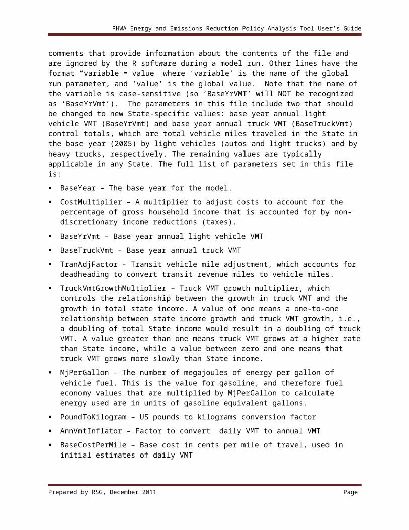
FHWA Energy and Emissions Reduction Policy Analysis Tool User’s Guide
LtVehDvmt – The values are the amount of VMT in each metropolitan area that is attributed to light vehicles, in units of thousands of miles. The analyst can develop these values using the data described for developing PropTruckDvmt, where the light vehicle VMT is the total VMT for each functional class in each metropolitan area minus the truck VMT. The LtVehDvmt is simply the sum of light vehicle VMT for all functional classes.
PropTruckDvmt – Heavy truck VMT needs to be attributed to metropolitan areas to calculate metropolitan congestion, which is done by applying the “PropTruckDvmt” proportions. The values are the proportion of total State truck VMT that takes place in each metropolitan area; the proportions sum to the proportion of total State truck VMT that takes places in all metropolitan areas in the State. The remaining proportion (i.e. 1 – proportion of VMT in metropolitan area) is the proportion of total State truck VMT that takes place in non-metropolitan areas. The analyst can develop these proportions by using base year (2005) State highway vehicle counts to allocate truck VMT between urbanized and non-urbanized areas. The Federal Highway Cost Allocation Study (Table II-6, 1997 Federal Highway Cost Allocation Study Final Report, Chapter II, http://www.fhwa.dot.gov/policy/hcas/final/two.htm) is used to calculate the average proportion of truck VMT by urban area functional class. The amount of the VMT in each metropolitan area that is truck-related is calculated by applying the proportions of truck VMT by functional class to HPMS estimates of VMT by functional class calculated for each metropolitan area. The proportions of total state truck VMT in each metropolitan area are then calculated from those results.
FwyArtProp – The values are the proportion of the VMT in each metropolitan area that takes place on freeways or arterials. The analyst can develop the proportions using urban area HPMS data by functional class and calculating the proportions of VMT using either freeway or arterial functional class roads.
Figure 18: File layout for mpo_base_dvmt_parm.csv (complete file shown)Area LtVehDvmt PropTruckDvmt FwyArtPropMetro 27244 0.191 0.77EugeneSpringfield 4112 0.0272 0.801SalemKeizer 3905 0.0282 0.85RogueValley 2783 0.019 0.743Bend 1423 0.008 0.738Corvallis 817 0.0046 0.728
7.1.11 pop_forecasts/pop_by_age_XXXX.csvFormat: This directory contains population estimates/forecasts by county and age cohort for each year (1990 to 2050 in 5-year intervals). The estimates/forecasts for each year are text files having the name “pop_by_age_XXXX.csv” where XXXX is the 4-digit year. Figure 19 shows the file layout, with one row per county and a column for each of the six age categories. The values are numbers of people.
Use: These files are used in the population synthesis model, which outputs the HsldXXXX.RData files. At the beginning of a model run, the model checks to see if the HsldXXXX.RData files exist and will not overwrite them if they do exist. Therefore, if the analyst updates the pop_by_age_XXXX.csv files and wants those changes to be reflected in the synthesized population used in subsequent model runs, the HsldXXXX.RData files should be deleted.
Prepared by RSG, December 2011 Page

FHWA Energy and Emissions Reduction Policy Analysis Tool User’s Guide
Source: These files are user created. The analyst can obtain Census data to develop the estimates for existing and past forecast years. In the Oregon application, population forecasts were provided by the Portland State University Center for Population Research and Census. The analyst can obtain State-specific population forecasts from similar data centers and/or academic sources in their State.
Figure 19: File layout for pop_by_age_XXXX.csv (partial file shown)County Age0to14 Age15to19 Age20to29 Age30to54 Age55to64 Age65PlusBaker 3494 914 1517 5007 1624 2865Benton 13633 7087 15708 23245 4521 6837Clackamas 63951 19236 34093 108875 22502 32216Clatsop 7356 2228 4075 11347 2983 5437Columbia 9273 2697 4209 13807 3113 4759Coos 12923 3784 6709 20205 6359 10423Crook 3298 997 1657 4665 1369 2252Curry 3498 913 1695 5993 2649 4705Deschutes 16916 4833 8798 28184 6846 10457…
7.1.12 transit_revenue_miles.csvFormat: transit_revenue_miles.csv is a table of annual bus and rail revenue miles7 per capita by metropolitan area. Figure 20 shows the file layout, with one row per metropolitan area and a column for each of bus, rail, and total revenue miles. The values are per capita revenue miles, i.e. total revenue miles divided by the population of the metropolitan area.
Use: The transit revenue miles are used to represent transit supply in the vehicle ownership model and vehicle use models and then are used in the calculations of transit vehicle emissions.
Source: This file is user created. The analyst can obtain these data from the National Transit Database (http://www.ntdprogram.gov/ntdprogram/data.htm)
Figure 20: File layout for transit_revenue_miles.csv (complete file shown)Msa Bus Rail TotalMetro 19 4 23EugeneSpringfield 18 0 18SalemKeizer 18 0 18RogueValley 10 0 10Bend 1 0 1Corvallis 5 0 5
7.1.13 truck_bus_fc_dvmt_split.csvFormat: truck_bus_fc_dvmt_split.csv is a table of proportions of truck and bus daily VMT by functional class. Figure 21 shows the file layout, with one row per metropolitan area for Bus VMT 7 “Transit revenue miles” represents the total distance traveled by the transit vehicles while in service, i.e. operating routes and available for passengers to travel on. This excludes miles traveled by the transit vehicles while not in service, e.g. traveling to/from depots to the start/end of routes.
Prepared by RSG, December 2011 Page

FHWA Energy and Emissions Reduction Policy Analysis Tool User’s Guide
followed by one row per metropolitan area for Truck VMT, and a column for proportions of VMT that take place on each of freeway, arterial, and other functional class roads.
Use: This file is used in calculations of the effects of metropolitan area congestion.
Source: This file is user created. The analyst can develop these data using Federal Highway Cost Allocation Study data, and data from transit authorities. The Federal Highway Cost Allocation Study (Table II-6, 1997 Federal Highway Cost Allocation Study Final Report, Chapter II, http://www.fhwa.dot.gov/policy/hcas/final/two.htm) is used to calculate the average proportion of truck VMT by urban area functional class, with the same values applied in each metropolitan area. Data from transit authorities are used to calculate the proportions of bus VMT by urban area functional class.
Figure 21: File layout for truck_bus_fc_dvmt_split.csv (complete file shown)Value Area Fwy Art OtherBusVmt Metro 0.15 0.591853844 0.258146156BusVmt EugeneSpringfield 0.05 0.661483708 0.288516292BusVmt SalemKeizer 0 0.69629864 0.30370136BusVmt RogueValley 0 0.69629864 0.30370136BusVmt Bend 0 0.69629864 0.30370136BusVmt Corvallis 0 0.69629864 0.30370136TruckVmt Metro 0.452028197 0.398645294 0.149326508TruckVmt EugeneSpringfield 0.452028197 0.398645294 0.149326508TruckVmt SalemKeizer 0.452028197 0.398645294 0.149326508TruckVmt RogueValley 0.452028197 0.398645294 0.149326508TruckVmt Bend 0.452028197 0.398645294 0.149326508TruckVmt Corvallis 0.452028197 0.398645294 0.149326508
7.1.14 ugb_areas.csvFormat: ugb_areas.csv is a table of geographic areas contained within urban boundaries (urban growth boundaries in States where those exist) defining metropolitan areas and other urban (town) areas by county. Figure 22 shows the file layout, with one row per county, and columns for metropolitan and town urban areas measured in square miles.
Use: The urban areas are used in calculations of urban densities.
Source: This file is user created. The analyst can develop these data using Census definitions of Urbanized Area boundaries based on Census block group population densities (http://www.census.gov/geo/www/cob/bdy_files.html), more recent population data to update 2000 data to 2005 data (such as county-level and incorporated place population estimates from the Census bureau, http://www.census.gov/popest/estbygeo.html), and State GIS data defining urban growth boundaries and/or urban areas. In States where there are no defined urban growth boundaries, the user can define the urban areas by means of the population density threshold used by the Census Bureau (areas with population density of 1000 persons or more per square mile). Where the high density urban area is part of a designated Urbanized Area, the area falls into the
Prepared by RSG, December 2011 Page

FHWA Energy and Emissions Reduction Policy Analysis Tool User’s Guide
“Metropolitan” category used in the FHWA tool. Where the high-density urban area is a smaller community outside any Urbanized Areas, then the area should be assigned to the “Town” category used in the FHWA tool. All remaining, non-urban land in each county should be designated as “Rural.”
Figure 22: File layout for ugb_areas.csv (partial file shown)County Metropolitan TownBaker 0 12.16549Benton 36.17008281 0.811709Clackamas 77.3122125 15.55516Clatsop 0 25.09685Columbia 0 19.20591Coos 0 31.10994Crook 0 8.31507Curry 0 15.78997Deschutes 32.39413281 16.85111…
7.1.15 urban_rural_pop_splits.csvFormat: urban_rural_pop_splits.csv is a table of the proportions of population located in the metropolitan, town, and rural portions of each county in the base year (2005). Figure 23 shows the file layout, with one row per county, and columns for the proportion of the population in metropolitan, town, and rural areas.
Use: This file is used to allocate the population from the county level to each of the three land use types.
Source: This file is user created. The analyst can develop these data using Census 2000 block group data (http://www.census.gov/main/www/cen2000.html), more recent population data to update 2000 data to 2005 data (such as county level and incorporated place population estimates from the Census bureau, http://www.census.gov/popest/estbygeo.html, or State sources of land use data), and the geographic definitions of urban and rural land use types discussed above under ugb_areas.csv.
Prepared by RSG, December 2011 Page

FHWA Energy and Emissions Reduction Policy Analysis Tool User’s Guide
Figure 23: File layout for urban_rural_pop_splits.csv (partial file shown)County Metropolitan Town RuralBaker 0 0.693433 0.306567Benton 0.745064169 0.065884 0.189052Clackamas 0.693735945 0.093422 0.212843Clatsop 0 0.628992 0.371008Columbia 0 0.522704 0.477296Coos 0 0.621211 0.378789Crook 0 0.53644 0.46356Curry 0 0.474523 0.525477Deschutes 0.498626124 0.130271 0.371103…
7.2 Scenarios Directory
The scenarios directory contains a directory for each scenario for which the FHWA tool is run. The inputs directory in each scenario directory must contain specific files described below. The “Designing Scenarios” section of this user’s guide discusses how to adjust these input files to set up alternative future scenarios.
age_adj.csv – Vehicle age adjustment factors by vehicle type and year auto_lighttruck_fuel.csv – Fuel type proportions for automobiles and light trucks auto_lighttruck_mpg.csv – Average fuel economy for automobiles and for light trucks by
vehicle model year bus_fuels.csv – Proportions of fuels used by buses carshare.csv – Availability rates for car-share vehicles costs.csv – Fuel and power costs for each forecast year eco_tire.csv – Participation/fuel economy benefits for eco-driving and low rolling resistance
tires ev_characteristics.csv – Information on electric vehicles for each vehicle model year fuel_co2.csv – CO2 equivalent emissions by fuel type fwy_art_growth.csv – Freeway lane mile growth and arterial lane mile growth heavy_truck_fuel.csv – Fuel type proportions for heavy trucks hvy_veh_mpg_mpk.csv – Average fuel economy and power economy for heavy vehicles light_vehicles.csv – Parameters for the light weight vehicle model lttruck_prop.csv – Proportion of the passenger vehicle fleet that is light trucks in each
forecast year metro_incident_reduction.csv – Incident reduction factors by metropolitan area and forecast
year metropolitan_urban_type_proportions.csv – Proportions of households in urban mixed-use
areas optimize.csv – Proportion of households who optimize their vehicle use parking.csv – Information on work place parking charges and other parking policy inputs payd.csv - Information describing Pay-as-You-Drive Insurance participation and costs per_cap_inc.csv – Statewide average per capita income by forecast year
Prepared by RSG, December 2011 Page
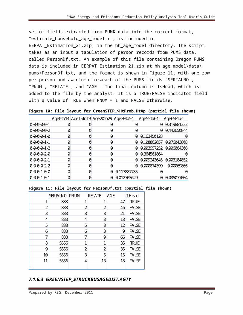
FHWA Energy and Emissions Reduction Policy Analysis Tool User’s Guide
phev_characteristics.csv - Information on plug-in hybrid electric vehicles for each vehicle model year
power_co2.csv – CO2 equivalents generated per kilowatt hour of electricity consumed regional_inc_prop.csv – Ratios of regional per capita income to statewide per capita income run_parameters.txt – Text file containing scenario details tdm.csv –Proportion of households reached TDM programs transit_growth.csv – Rates of transit revenue mile growth ugb_area_growth_rates.csv – Growth rates of urban growth boundary areas urban_rural_growth_splits.csv – Proportions of population growth by area type
7.2.1 age_adj.csvFormat: age_adj.csv contains a table of vehicle age adjustment factors by vehicle type and forecast year. Figure 24 shows the file layout, with one row per forecast year from 1990 to 2050 in 5-year increments, and a column for auto, light truck, truck, and bus. The data are adjustment factors that can be varied around 1.0.
Use: The purpose of this input is to allow scenarios to be developed that test faster (or slower) turnover of the vehicle fleet. The age adjustment factors identify how much the 95th percentile vehicle fleet age is to be adjusted from that of the current vehicle fleet based on recent State DMV data (the data that were used to develop the cumulative distribution of auto and light truck ages tabulation in VehProp_ described in Section 7.1.6). For example, a value of 0.9 would adjust the 95th
percentile age to be 0.9 times the current value. If the current 95th percentile age is 20 years, then applying this adjustment factor to a forecast year would show the 95th percentile age for that year to be 18 years. The FHWA tool alters the entire age distribution to be consistent with the adjusted 95th percentile age. Figure 24 shows how to represent cases where historical fleet turnover was slower than the current rate of fleet turnover. For the Oregon implementation, the current age distributions were based on 2009 State DMV data; historical data showed that the 95th percentile vehicle fleet age varied between 10% and 30% higher between 1990 and 2005.
Source: This file is user created.
Prepared by RSG, December 2011 Page

FHWA Energy and Emissions Reduction Policy Analysis Tool User’s Guide
Figure 24: File layout for age_adj.csv (complete file shown)Year Auto LtTruck Truck Bus
1990 1.1 1.1 1 11995 1.3 1.2 1 12000 1.3 1.3 1 12005 1.1 1.1 1 12010 1 1 1 12015 1 1 1 12020 1 1 1 12025 1 1 1 12030 1 1 1 12035 1 1 1 12040 1 1 1 12045 1 1 1 12050 1 1 1 1
7.2.2 auto_lighttruck_fuel.csvFormat: auto_lighttruck_fuel.csv contains a table of fuel type proportions for automobiles and light trucks for the forecast years. Figure 25 shows the file layout; the table fields are as follows. The remaining proportion of fuel not accounted for in these categories is assumed to be gasoline:
Year – The forecast year (i.e. 1990 to 2050 in 5-year increments) AutoPropDiesel – The proportion of the automobile fleet that uses diesel AutoPropCng – The proportion of the auto fleet that uses compressed natural gas LtTrkPropDiesel – The proportion of the light truck fleet that uses diesel LtTrkPropCng – The proportion of the light truck fleet that uses compressed natural gas GasPropEth – The average ethanol proportion in gasoline sold DieselPropBio – The average biodiesel proportion in diesel sold.
Use: This file is used in the calculations of fuel consumption. This file can be used to test alternative fuel scenarios by varying the future shares of non-gasoline fuels.
Source: This file is user created.
Using MOVES inputs: MOVES uses fuel supply, fuel formulation, and engine fuel type inputs (FuelSupply, FuelFormulation, and FuelEngFraction) that can be used to derive the simpler fuel inputs required by the FHWA tool. The engine fuel type table contains the joint distribution of vehicle types and fuel types, from which the proportion of autos and light trucks that use diesel can be extracted. The fuel supply and fuel formulation tables can be used to derive the average ethanol proportion in gasoline and, if a user-defined biodiesel blend had been added to the State MOVES model being referenced by the analyst, the average biodiesel proportion in diesel.
Prepared by RSG, December 2011 Page

FHWA Energy and Emissions Reduction Policy Analysis Tool User’s Guide
Figure 25: File layout for auto_lighttruck_fuel.csv (complete file shown)Year AutoPropDiesel AutoPropCng LtTrkPropDiesel LtTrkPropCng GasPropEth DieselPropBio
1990 0.007 0 0.04 0 0 01995 0.007 0 0.04 0 0 02000 0.007 0 0.04 0 0 02005 0.007 0 0.04 0 0.1 0.052010 0.007 0 0.04 0 0.1 0.052015 0.007 0 0.04 0 0.1 0.052020 0.007 0 0.04 0 0.1 0.052025 0.007 0 0.04 0 0.1 0.052030 0.007 0 0.04 0 0.1 0.052035 0.007 0 0.04 0 0.1 0.052040 0.007 0 0.04 0 0.1 0.052045 0.007 0 0.04 0 0.1 0.052050 0.007 0 0.04 0 0.1 0.05
7.2.3 auto_lighttruck_mpg.csvFormat auto_lighttruck_mpg.csv contains estimates and forecasts of average fuel economy in miles per gallon for automobiles and for light trucks by vehicle model year. Note that this is not the fleet average. It is the average for new vehicles sold in the year. The fuel economy is the same for all fuel types and is measured in gasoline equivalent gallons (i.e. energy content of a gallon of gasoline). Figure 26 shows the file layout, with one row for each year from 1975 to 2050.
Use: This file is used in the calculations of fuel consumption. This file can be used to test alternative vehicle development scenarios, such as improved technology and/or fuel economy standards that lead to higher vehicle fuel economies.
Source: This file is user created.
Using MOVES input/output: MOVES emissions inventory results can be used to calculate an average fuel economy by vehicle type and vehicle model year. Fuel economy is the quantity of miles traveled per unit of fuel used (in gallons). MOVES calculates total energy consumed by vehicle type and vehicle age based on inputs of miles traveled for each vehicle type and vehicle age. The ratio of miles traveled/mJ of energy consumed for each vehicle type and vehicle age can be converted to fuel economy based on the assumption for energy content per gallon of gasoline used in the FHWA tool of 121 mJ/gallon (the single value for gasoline is used irrespective of fuel type, which means that the conversion is to fuel economy in gasoline equivalent gallons). The MOVES vehicle types to use for this input file are:
MOVES SourceType 21, Passenger Car, is equivalent to autos in the FHWA tool
MOVES Source Type 31, Passenger Truck, is equivalent to light truck in the FHWA tool.
Prepared by RSG, December 2011 Page

FHWA Energy and Emissions Reduction Policy Analysis Tool User’s Guide
Figure 26: File layout for auto_lighttruck_mpg.csv (partial file shown)Year Auto LtTruck
1975 15.1 12.71976 16.6 13.21977 17.4 14.11978 19.2 13.71979 19.3 13.11980 22.6 17.11981 24.2 18.61982 25.6 19
…2050 63.7 41.1
7.2.4 bus_fuels.csvFormat: bus_fuels.csv contains estimates and forecasts of the proportions of fuels used by buses. Figure 27 shows the file layout, with four rows (one for each fuel type) for each metropolitan area, and columns for each forecast year from 1990 to 2050. For each metropolitan area and each forecast year, the following proportions are specified:
PropGas – The proportion of bus miles using gasoline PropGng – The proportion of bus miles using compressed natural gas DieselPropBio – The biodiesel proportion of diesel fuel used GasPropEth – The ethanol proportion of gasoline used.
Use: This file is used in the calculations of fuel consumption. The future values can be varied to test alternative bus fueling scenarios such as investments in CNG-fueled buses.
Source: This file is user created. Historical data can be obtained from metropolitan bus operators and/or transit authorities.
Using MOVES inputs: MOVES uses fuel supply, fuel formulation, and engine fuel type inputs (FuelSupply, Fuel Formulation, and FuelEngFraction) that can be used to derive the simpler fuel inputs required by the FHWA tool. The engine fuel type table contains the joint distribution of vehicle types and fuel types, from which the proportion of buses that use gasoline or compressed natural gas can be extracted. The fuel supply and fuel formulation tables can be used to derive the average ethanol proportion in gasoline and the average biodiesel proportion in diesel.
Prepared by RSG, December 2011 Page

FHWA Energy and Emissions Reduction Policy Analysis Tool User’s Guide
Figure 27: File layout for bus_fuels.csv (partial file shown)Area Fuel 1990 1995 2000 2005 … 2050Metro PropGas 0 0 0 0 0Metro PropCng 0.039574 0.039574 0.039574 0.039574 0.039574Metro DieselPropBio 0 0 0.05 0.05 0.05Metro GasPropEth 0 0 0.05 0.1 0.1EugeneSpringfield PropGas 0 0 0 0 0EugeneSpringfield PropCng 0 0 0 0 0EugeneSpringfield DieselPropBio 0 0 0 0 0EugeneSpringfield GasPropEth 0 0 0.05 0.1 0.1…
7.2.5 carshare.csvFormat: carshare.csv is a table showing the availability of car-share vehicles in terms of the population per car-share vehicle in medium- (4,000-10,000 people per square mile) and high- density (>10,000 people per square mile) portions of metropolitan areas. Figure 28 shows the file layout, with one row per metropolitan area for each of medium-density and high-density areas. There is one column for each forecast year by 5-year intervals from 1990 to 2050. The units of the rates are persons per car-share vehicle.
Use: The representation of car-sharing is discussed in the FHWA Tool Model Documentation in Section 13.1 “Car-Sharing.”
Source: This file is user created.
Figure 28: File layout for carshare.csv (partial file shown)Value Area 1990 1995 2000 2005 … 2050MedDenRate Bend 50000 50000 50000 50000 50000MedDenRate Corvallis 50000 50000 50000 50000 50000MedDenRate EugeneSpringfield 50000 50000 50000 50000 20000MedDenRate Metro 50000 50000 50000 20000 10000MedDenRate RogueValley 50000 50000 50000 50000 50000MedDenRate SalemKeizer 50000 50000 50000 50000 20000HighDenRate Bend 50000 50000 50000 50000 50000HighDenRate Corvallis 50000 50000 50000 50000 50000HighDenRate EugeneSpringfield 50000 50000 50000 25000 10000HighDenRate Metro 50000 50000 25000 10000 5000HighDenRate RogueValley 50000 50000 50000 50000 50000HighDenRate SalemKeizer 50000 50000 50000 25000 50000
7.2.6 costs.csvFormat: costs.csv contains information on fuel and power costs in year 2000 dollars for each forecast year. Figure 29 shows the file layout, with one row per forecast year and columns for various types of vehicle fuel costs or charges. The table fields are as follows:
Prepared by RSG, December 2011 Page

FHWA Energy and Emissions Reduction Policy Analysis Tool User’s Guide
Year – The forecast year (i.e. 1990 to 2050 in 5-year increments) FuelCost – The average cost of gasoline and diesel fuels excluding tax KwhCost – The average cost of electricity per kilowatt hour VmtCost – The cost of taxes for vehicle miles traveled CarbonCost – The cost of taxes for any carbon emissions GasTax – The average cost of gasoline and diesel fuel taxes.
Use: The costs in this file can be used to test various vehicle travel cost scenarios, such as VMT fees. The FHWA Tool Model Documentation, in Section 12 “Modeling the Effects of Vehicle Travel Costs on Household Vehicle Travel” explains how daily vehicle travel is affected by these costs.
Source: This file is user created.
Figure 29: File layout for costs.csv (complete file shown)Year FuelCost KwhCost VmtCost CarbonCost GasTax
1990 1.23 0.075 0 0 0.4241995 1.06 0.075 0 0 0.4242000 1.25 0.075 0 0 0.4242005 1.82 0.075 0 0 0.4242010 2.38 0.075 0 0 0.4242015 3.02 0.135 0 0 0.4242020 3.32 0.157 0 0 0.4242025 3.5 0.175 0 0 0.4242030 3.71 0.185 0 0 0.4242035 3.97 0.19 0 0 0.4242040 4.2 0.193 0 0 0.4242045 4.44 0.193 0 0 0.4242050 4.68 0.193 0 0 0.424
7.2.7 eco_tire.csvFormat: eco_tire.csv contains information on the proportion of households participating in eco-driving practices and the proportion of households that use low rolling resistance tires. Figure 30 shows the file layout, with one row for each forecast year and the following columns:
Year – The forecast year (i.e. 1990 to 2050 in 5-year increments) EcoDrvProp – The proportion of households participating in eco-driving practices LowRollProp – The proportion of households that use low rolling resistance tires EcoMpgImp – The increase in fuel economy for internal combustion engines (as a
proportion) as a result of eco-driving EcoMpkwhImp – The increase in miles per kWh for electric vehicles (as a proportion) as a
result of eco-driving TireMpgImp – The increase in fuel economy for internal combustion engines (as a
proportion) as a result of using low rolling resistance tires TireMpkwhImp – The increase in miles per kWh for electric vehicles (as a proportion) as a
result of using low rolling resistance tires.
Prepared by RSG, December 2011 Page
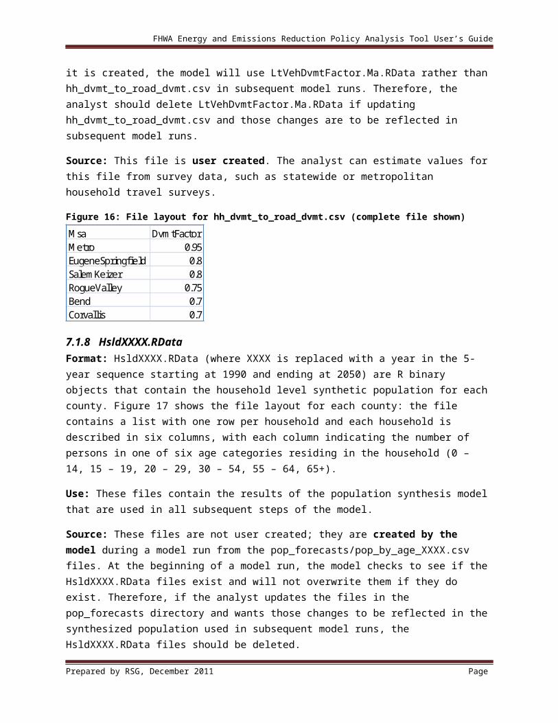
FHWA Energy and Emissions Reduction Policy Analysis Tool User’s Guide
Use: This file is used in the calculations of fuel consumption and electricity consumption to modify average fuel economy. The participation rates can be adjusted to test the effect of policies to increase eco-driving and use of low rolling resistance tires.
Source: This file is user created. The FHWA Tool Model Documentation (in Section 13.8 “Eco-Driving” and Section 13.9 “Low Rolling Resistance Tires”) discusses research into the effectiveness of both eco-driving practices and the low rolling resistance tires that can be used as references for developing the values in this file, including information in the “Moving Cooler” study8 and TRB Special Report 286 “Tires and Passenger Vehicle Fuel Economy.”9
Figure 30: File layout for eco_tire.csv (complete file shown)Year EcoDrvProp LowRollProp EcoMpgImp EcoMpkwhImp TireMpgImp TireMpkwhImp
1990 0 0 0.03 0.03 0.01 0.011995 0 0 0.03 0.03 0.01 0.012000 0 0 0.03 0.03 0.01 0.012005 0 0 0.03 0.03 0.01 0.012010 0 0 0.03 0.03 0.01 0.012015 0 0 0.03 0.03 0.01 0.012020 0 0 0.03 0.03 0.01 0.012025 0 0 0.03 0.03 0.01 0.012030 0 0 0.03 0.03 0.01 0.012035 0 0 0.03 0.03 0.01 0.012040 0 0 0.03 0.03 0.01 0.012045 0 0 0.03 0.03 0.01 0.012050 0 0 0.03 0.03 0.01 0.01
7.2.8 ev_characteristics.csvFormat: ev_characteristics.csv contains information on electric vehicles for each vehicle model year. Figure 31 shows the file layout, with one row for each vehicle model year (1975 to 2050). The fields are as follows:
Year – The vehicle model year AutoRange – The average vehicle range (between charges) for electric automobiles in the
vehicle model year AutoPropEv – The proportion of autos for each vehicle model year driven on average within
the range of electric vehicles that are electric vehicles. For example, if the average electric vehicle range for the year 2030 is 100 miles and the AutoPropEv value for 2030 is 0.5, then half of the automobiles that travel on average less than or equal to 100 miles in a day are assumed to be electric vehicles
AutoMpkwh – The average power efficiency of electric automobiles for the vehicle model year in miles per kilowatt hour
8 Cambridge Systematics, “Moving Cooler,” Urban Land Institute, Washington, D.C., 2009, Technical Appendix, Table 7.1, page B-63.9 Transportation Research Board, “Tires and Passenger Vehicle Fuel Economy,” Special Report 286, Transportation Research Board, Washington, D.C., 2006.
Prepared by RSG, December 2011 Page

FHWA Energy and Emissions Reduction Policy Analysis Tool User’s Guide
LtTruckRange – The average vehicle range for electric light trucks for each vehicle model year
LtTruckPropEv – Same data as for AutoPropEv but for light trucks LtTruckMpkwh – Same data as for AutoMpkwh but for light trucks.
Use: This file is used to assign the number of electric vehicles in the Electric Vehicle Model. The electric vehicle model assigns electric vehicle ownership using a Monte Carlo process from amongst the pool of electric vehicle candidates, i.e. all plug-in hybrid electric vehicles. The values in the file can be adjusted to test alternative electric vehicle scenarios, such as higher electric vehicle market shares or technological improvements that increase vehicle range.
Source: This file is user created.
Figure 31: File layout for ev_characteristics.csv (partial file shown)Year AutoRange AutoPropEv AutoMpkwh LtTruckRange LtTruckPropEv LtTruckMpkwh
1975 0 0 3 0 0 21976 0 0 3 0 0 21977 0 0 3 0 0 21978 0 0 3 0 0 21979 0 0 3 0 0 21980 0 0 3 0 0 21981 0 0 3 0 0 21982 0 0 3 0 0 2
…
7.2.9 fuel_co2.csvFormat: fuel_co2.csv contains information on “pump-to-wheels” CO2 equivalent emissions by fuel type in grams per mega Joule of fuel energy content. Figure 32 shows the file layout, with one row for each forecast year (1990 to 2050 in 5-year increments) and columns for each fuel type: ULSD (ultra low-sulfur diesel), biodiesel, RFG (reformulated gasoline), CARBOB (gasoline formulated to be blended with ethanol), ethanol, CNG (compressed natural gas), and light vehicle composite fuel.
Use: This file is used to convert fuel use to CO2 equivalent emissions. The “pump-to-wheels” rates do not vary by State and so the values provided in the table can be used for any application of the FHWA tool.
Source: This file is user created.
Using MOVES inputs/outputs: The FHWA tool is consistent with MOVES in that it produces calculations for “pump-to-wheels” CO2 equivalent emissions. However, the estimate of the portion of CO2 equivalent emissions that comes from sources other than CO2 (i.e. CH4, N2O, and HFCs) is an approximation and can be calculated in more detail using MOVES.
Prepared by RSG, December 2011 Page

FHWA Energy and Emissions Reduction Policy Analysis Tool User’s Guide
The calculation of rates for CO2 equivalent emissions is discussed in the Draft MOVES 2009 Software Design and Reference Manual,10 with the calculation of energy consumption explained in Section 10.17, and the calculation of CO2 equivalent emissions discussed in Section 10.20. The rates used in the FHWA tool are CO2 equivalent emissions by fuel type in grams per mega Joule of fuel energy content; these could be derived from MOVES by taking the ratio of CO2 equivalent emissions and energy consumption for each fuel type.
Figure 32: File layout for fuel_co2.csv (complete file shown)Year ULSD Biodiesel RFG CARBOB Ethanol Cng LtVehComposite
1990 77.19 76.81 75.65 75.65 74.88 62.14 75.691995 77.19 76.81 75.65 75.65 74.88 62.14 75.692000 77.19 76.81 75.65 75.65 74.88 62.14 75.692005 77.19 76.81 75.65 75.65 74.88 62.14 75.612010 77.19 76.81 75.65 75.65 74.88 62.14 75.612015 77.19 76.81 75.65 75.65 74.88 62.14 75.612020 77.19 76.81 75.65 75.65 74.88 62.14 75.612025 77.19 76.81 75.65 75.65 74.88 62.14 75.612030 77.19 76.81 75.65 75.65 74.88 62.14 75.612035 77.19 76.81 75.65 75.65 74.88 62.14 75.612040 77.19 76.81 75.65 75.65 74.88 62.14 75.612045 77.19 76.81 75.65 75.65 74.88 62.14 75.612050 77.19 76.81 75.65 75.65 74.88 62.14 75.61
7.2.10 fwy_art_growth.csvFormat: fwy_art_growth.csv contains information about rates of freeway lane mile growth and arterial lane mile growth relative to population for each metropolitan area. For example, a value of 0.5 for arterials means that arterial lane miles are assumed to grow at half the rate of population growth. Figure 33 shows the file layout, with one row per metropolitan area and columns for freeways and arterials.
Use: This file is used to calculate transportation supply in terms of lane miles for freeways and arterials in metropolitan areas in the future. The data are used in the vehicle ownership and vehicle use models and in the models and calculations that adjust metropolitan area fuel economy to account for congestion.
Source: This file is user created.
10 http://www.epa.gov/otaq/models/moves/420b09007.pdf
Prepared by RSG, December 2011 Page

FHWA Energy and Emissions Reduction Policy Analysis Tool User’s Guide
Figure 33: File layout for fwy_art_growth.csv (complete file shown)Msa Fwy ArtMetro 0.24 0.21EugeneSpringfield 0.1 0.11SalemKeizer 0.97 0.23RogueValley 0 0.11Bend 0 0.1Corvallis 0 0.35
7.2.11 heavy_truck_fuel.csvFormat: heavy_truck_fuel.csv contains a table of fuel type proportions for heavy trucks for the forecast years. Figure 34 shows the file layout, with one row for each forecast year. The table fields are as follows; the remaining fuel is assumed to be diesel fuel:
Year – The forecast year (i.e. 1990 to 2050 in 5-year increments) PropGas – The proportion of heavy trucks using gasoline PropCng – The proportion of heavy trucks using compressed natural gas GasPropEth – The ethanol proportion of gasoline used DieselPropBio – The biodiesel proportion of diesel fuel used.
Use: This file is used in the calculations of fuel consumption. This file can be used to test alternative fuel scenarios by varying the future shares of non-diesel fuels.
Source: This file is user created.
Using MOVES inputs: MOVES uses fuel supply, fuel formulation, and engine fuel type inputs (FuelSupply, Fuel Formulation, and FuelEngFraction) that can be used to derive the simpler fuel inputs required by the FHWA tool. The engine fuel type table contains the joint distribution of vehicle types and fuel types, from which the proportion of trucks that use gasoline or compressed natural gas can be extracted. The fuel supply and fuel formulation tables can be used to derive the average ethanol proportion in gasoline and the average biodiesel proportion in diesel.
Prepared by RSG, December 2011 Page

FHWA Energy and Emissions Reduction Policy Analysis Tool User’s Guide
Figure 34: File layout for heavy_truck_fuel.csv (complete file shown)Year PropGas PropCng GasPropEth DieselPropBio
1990 0.05 0 0 01995 0.05 0 0 02000 0.05 0 0 02005 0.05 0.005 0.1 0.012010 0.05 0.005 0.1 0.052015 0.05 0.005 0.1 0.052020 0.05 0.01 0.1 0.052025 0.05 0.01 0.1 0.052030 0.05 0.01 0.1 0.052035 0.05 0.015 0.1 0.052040 0.05 0.015 0.1 0.052045 0.05 0.015 0.1 0.052050 0.05 0.015 0.1 0.05
7.2.12 hvy_veh_mpg_mpk.csvFormat: hvy_veh_mpg_mpk.csv contains estimates and forecasts of average fuel economy and power economy in miles per gallon and miles per kilowatt hour for heavy vehicles (heavy truck, bus, train) by vehicle model year. Note that this is not the fleet average. It is the average for new vehicles sold in the year. The fuel economy is the same for all fuel types and is measured in gasoline equivalent gallons (i.e. energy content of a gallon of gasoline). Figure 35 shows the file layout, with one row per vehicle model year (1975 to 2050).
Use: This file is used in the calculations of fuel consumption. This file can be used to test alternative vehicle development scenarios, such as improved technology and/or fuel economy standards that lead to higher vehicle fuel economies.
Source: This file is user created.
Using MOVES input/output: MOVES emissions inventory results can be used to calculate an average fuel economy by vehicle type and vehicle model year. Fuel economy is the quantity of miles traveled per unit of fuel used (in gallons). MOVES calculates total energy consumed by vehicle type and vehicle age based on inputs of miles traveled for each vehicle type and vehicle age. The ratio of miles traveled/mJ of energy consumed for each vehicle type and vehicle age can be converted to fuel economy using the assumption for energy content per gallon of gasoline used in the FHWA tool of 121 mJ/gallon (the single value for gasoline is used irrespective of fuel type, which means that the conversion is to fuel economy in gasoline equivalent gallons). The MOVES vehicle types to use for this input file are:
MOVES Source Type 42, “Transit Bus,” is equivalent to bus in the FHWA tool
MOVES Source Type 51-53 and 61-62 are equivalent to heavy trucks in the FHWA tool and their distributions should be combined (weighting by the vehicle population of each of the SourceTypes in SourceTypeYear).
Prepared by RSG, December 2011 Page
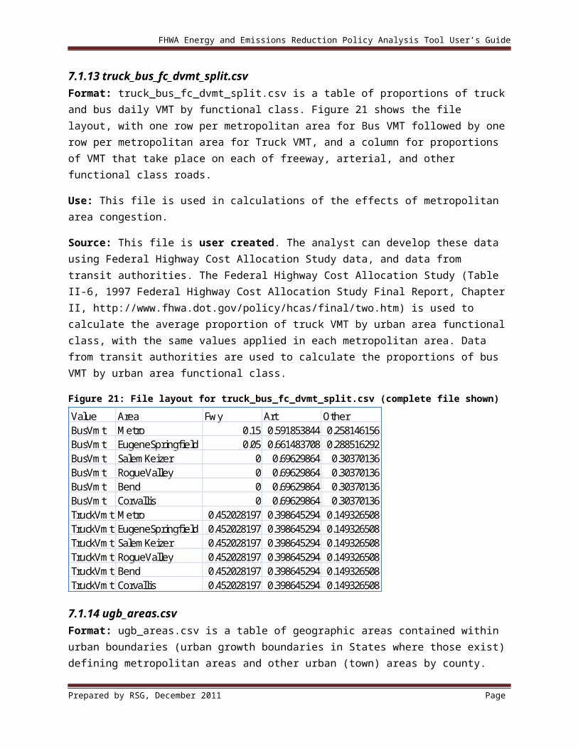
FHWA Energy and Emissions Reduction Policy Analysis Tool User’s Guide
Figure 35: File layout for hvy_veh_mpg_mpk.csv (partial file shown)Year Truck Bus Train
1975 5.1 4.2 0.0982661976 5.1 4.1 0.0982661977 5.1 4.1 0.0982661978 5.1 4 0.0982661979 5.1 3.9 0.0982661980 5.3 3.9 0.0982661981 5.1 3.8 0.0982661982 5.2 3.8 0.098266
…
7.2.13 light_vehicles.csvFormat: light_vehicles.csv contains input data for the non-motorized vehicle model. In the FHWA tool, non-motorized vehicles are bicycles, and also electric bicycles, Segways, and similar vehicles that are small, light-weight and can travel at bicycle speeds or slightly higher. Figure 36 shows the file layout, with one row per metropolitan area plus a row for non metropolitan areas, for each of “TargetProp”, “Threshold” and “PropSuitable”, and columns for each forecast year (1990 to 2050 in 5-year increments).
TargetProp – non-motorized vehicle ownership rate (average ratio of non-motorized vehicles to driver age population)
Threshold – SOV tour mileage threshold used in the SOV travel proportion model PropSuitable – proportion of SOV travel suitable for non-motorized vehicle travel.
Use: This file is used in the light vehicle model, which is described in the FHWA Tool Model Documentation in Section 15 “Non-Motorized Vehicle Model.” This section includes the SOV travel proportion model. This file can be used to define and test scenarios where ownership of non-motorized increases in the future.
Source: This file is user created.
Prepared by RSG, December 2011 Page

FHWA Energy and Emissions Reduction Policy Analysis Tool User’s Guide
Figure 36: File layout for light_vehicles.csv (partial file shown)Value Area 1990 1995 2000 2005 … 2050TargetProp Bend 0.2 0.2 0.2 0.2 0.2TargetProp Corvallis 0.2 0.2 0.2 0.2 0.2TargetProp EugeneSpringfield 0.2 0.2 0.2 0.2 0.2TargetProp Metro 0.2 0.2 0.2 0.2 0.2TargetProp RogueValley 0.2 0.2 0.2 0.2 0.2TargetProp SalemKeizer 0.2 0.2 0.2 0.2 0.2TargetProp NonMetro 0.2 0.2 0.2 0.2 0.2Threshold Bend 2 2 2 2 2Threshold Corvallis 2 2 2 2 2Threshold EugeneSpringfield 2 2 2 2 2Threshold Metro 2 2 2 2 2Threshold RogueValley 2 2 2 2 2Threshold SalemKeizer 2 2 2 2 2Threshold NonMetro 2 2 2 2 2PropSuitable Bend 0.1 0.1 0.1 0.1 0.1PropSuitable Corvallis 0.1 0.1 0.1 0.1 0.1PropSuitable EugeneSpringfield 0.1 0.1 0.1 0.1 0.1PropSuitable Metro 0.1 0.1 0.1 0.1 0.1PropSuitable RogueValley 0.1 0.1 0.1 0.1 0.1PropSuitable SalemKeizer 0.1 0.1 0.1 0.1 0.1PropSuitable NonMetro 0.1 0.1 0.1 0.1 0.1
7.2.14 lttruck_prop.csvFormat: lttruck_prop.csv contains targets for the proportion of the passenger vehicle fleet that is light trucks in each forecast year. The FHWA tool will compute the proportion based on year 2000 household behavior where the input value is “NA”. If a number (between 0 and 1) is input, the FHWA tool will make adjustments to match the target value instead. Figure 37 shows the file layout, with one row for each county and columns for each forecast year (1990 to 2050 in 5-year increments).
Use: This file is used in the vehicle type model. This file can be used to explore the effects of different vehicle buying preferences, in terms of light trucks vs. autos, in the future.
Source: This file is user created.
Using MOVES inputs: The proportion of the passenger vehicle fleet that is light trucks can be calculated from MOVES vehicle population data (SourceTypeYear) derived from local registration data. The vehicle types used in MOVES (SourceType) correspond with the two categories of passenger vehicles used in the FHWA tool: MOVES SourceType 21, Passenger Car, is equivalent to autos in the FHWA tool and MOVES Source Type 31, Passenger Truck, is equivalent to light trucks.
Prepared by RSG, December 2011 Page

FHWA Energy and Emissions Reduction Policy Analysis Tool User’s Guide
Figure 37: File layout for lttruck_prop.csv (partial file shown)County 1990 1995 2000 2005 … 2050Baker 0.44 0.51 0.58 0.62 0.63Benton 0.33 0.39 0.44 0.47 0.48Clackamas 0.35 0.41 0.47 0.5 0.51Clatsop 0.4 0.46 0.53 0.56 0.57Columbia 0.38 0.44 0.5 0.53 0.54Coos 0.41 0.48 0.55 0.58 0.59Crook 0.44 0.52 0.59 0.63 0.64Curry 0.42 0.49 0.56 0.59 0.6Deschutes 0.42 0.49 0.56 0.6 0.61…
7.2.15 metro_incident_reduction.csvFormat: metro_incident_reduction.csv contains a table of incident reduction factors by metropolitan area and forecast year. The values need to be between 0 and 1 where 0 means no incident reduction and 1 means that all incidents have been eliminated. Figure 38 shows the file layout, with one row for each forecast year (1990 to 2050 in 5-year increments) and one column for each metropolitan area.
Use: This file is used in calculations of the effects of metropolitan area congestion. The calculations use the values to interpolate between mean speeds with and without incidents to compute an overall average speed by road type and congestion level. The approach provides a simple level of sensitivity testing of the potential effects of incident management programs on emissions.
Source: This file is user created.
Figure 38: File layout for metro_incident_reduction.csv (complete file shown)Year Bend Corvallis EugeneSpringfield Metro RogueValley SalemKeizer
1990 0 0 0 0 0 01995 0 0 0 0 0 02000 0 0 0 0 0 02005 0 0 0 0 0 02010 0 0 0.02 0.1 0 0.022015 0 0 0.02 0.1 0 0.022020 0 0 0.02 0.1 0 0.022025 0 0 0.02 0.1 0 0.022030 0 0 0.02 0.1 0 0.022035 0 0 0.02 0.1 0 0.022040 0 0 0.02 0.1 0 0.022045 0 0 0.02 0.1 0 0.022050 0 0 0.02 0.1 0 0.02
Prepared by RSG, December 2011 Page

FHWA Energy and Emissions Reduction Policy Analysis Tool User’s Guide
7.2.16 metropolitan_urban_type_proportions.csvFormat: metropolitan_urban_type_proportions.csv contains a table of household proportions that are located in urban mixed-use areas by metropolitan area and forecast year. The FHWA tool will compute the proportion based on year 2000 household characteristics where the input value is “NA”. If a number (between 0 and 1) is input, the FHWA tool will make adjustments to match the target value instead. Figure 39 shows the file layout, with one row for each forecast year (1990 to 2050 in 5-year increments) and one column for each metropolitan area.
Use: This file is used in the household daily VMT model to account for the reduced VMT generated by households that live in mixed-use areas. The file can be used to test the effects of land use development policies that facilitate and encourage mixed-use development.
Source: This file is user created.
Figure 39: File layout for metropolitan_urban_type_proportions.csv (complete file shown)Year Bend Corvallis EugeneSpringfield Metro RogueValley SalemKeizer
1990 NA NA NA NA NA NA1995 NA NA NA NA NA NA2000 NA NA NA NA NA NA2005 0.25 0.25 0.25 0.35 0.25 0.252010 0.25 0.25 0.25 0.35 0.25 0.252015 0.25 0.25 0.25 0.35 0.25 0.252020 0.25 0.25 0.25 0.35 0.25 0.252025 0.25 0.25 0.25 0.35 0.25 0.252030 0.25 0.25 0.25 0.4 0.25 0.252035 0.25 0.25 0.25 0.4 0.25 0.252040 0.25 0.25 0.25 0.4 0.25 0.252045 0.25 0.25 0.25 0.4 0.25 0.252050 0.25 0.25 0.25 0.4 0.25 0.25
7.2.17 optimize.csvFormat: optimize.csv contains information on the proportion of households that optimize, i.e. that consciously use, the most fuel efficient vehicle that is available to them for a given trip. Figure 40 shows the file layout, with one row for each forecast year (1990 to 2050 in 5-year increments).
Use: This file is used in the calculations to allocate household DVMT to different household vehicles. The file can be used to test scenarios for different levels of optimizing behavior in the population.
Source: This file is user created.
Prepared by RSG, December 2011 Page

FHWA Energy and Emissions Reduction Policy Analysis Tool User’s Guide
Figure 40: File layout for optimize.csv (complete file shown)Year OptimProp
1990 01995 02000 02005 02010 02015 02020 02025 02030 02035 02040 02045 02050 0
7.2.18 parking.csvFormat: parking.csv contains information that allows the effects of policies such as workplace parking charges and “cash-out buy-back” programs to be tested. Figure 41 shows the file layout, with rows for each metropolitan area for a set of input parameters, and columns for each forecast year (1990 to 2050 in 5-year increments). The input parameters are as follows:
PropWrkPkg – proportion of employees that park at work PropWrkChrgd – proportion of employers that charge for parking PropCashOut – proportion of employment parking that is converted from being free to pay
under a “cash-out buy-back” type of program PrkOthChrgd – proportion of other parking that is not free PkgCost – average daily parking cost.
Use: This file is used to test the effects of policies such as workplace parking charges and “cash-out buy-back” programs. The policies are discussed in the FHWA Tool Model Documentation in Section 13.6 “Parking Pricing”.
Source: This file is user created.
Prepared by RSG, December 2011 Page

FHWA Energy and Emissions Reduction Policy Analysis Tool User’s Guide
Figure 41: File layout for parking.csv (partial file shown)Value Area 1990 1995 2000 2005 … 2050PropWrkPkg Bend 0 0 0 0 0PropWrkPkg Corvallis 0 0 0 0 0PropWrkPkg EugeneSpringfield 0.75 0.75 0.75 0.75 0.75PropWrkPkg Metro 1 1 1 1 1PropWrkPkg RogueValley 0 0 0 0 0PropWrkPkg SalemKeizer 0.75 0.75 0.75 0.75 0.75PropWrkChrgd Bend 0 0 0 0 0PropWrkChrgd Corvallis 0 0 0 0 0PropWrkChrgd EugeneSpringfield 0.1 0.1 0.1 0.1 0.1PropWrkChrgd Metro 0.1 0.1 0.1 0.1 0.1PropWrkChrgd RogueValley 0 0 0 0 0PropWrkChrgd SalemKeizer 0.1 0.1 0.1 0.1 0.1PropCashOut Bend 0 0 0 0 0PropCashOut Corvallis 0 0 0 0 0PropCashOut EugeneSpringfield 0 0 0 0 0PropCashOut Metro 0 0 0 0 0PropCashOut RogueValley 0 0 0 0 0PropCashOut SalemKeizer 0 0 0 0 0PropOthChrgd Bend 0 0 0 0 0PropOthChrgd Corvallis 0 0 0 0 0PropOthChrgd EugeneSpringfield 0.05 0.05 0.05 0.05 0.05PropOthChrgd Metro 0.05 0.05 0.05 0.05 0.05PropOthChrgd RogueValley 0 0 0 0 0PropOthChrgd SalemKeizer 0.05 0.05 0.05 0.05 0.05PkgCost Bend 0 0 0 0 0PkgCost Corvallis 0 0 0 0 0PkgCost EugeneSpringfield 1 1 1 1 1PkgCost Metro 5 5 5 5 5PkgCost RogueValley 0 0 0 0 0PkgCost SalemKeizer 2.5 2.5 2.5 2.5 2.5
7.2.19 payd.csvFormat: payd.csv contains information describing Pay-as-You-Drive Insurance participation and costs. Figure 42 shows the file layout, with one row for each forecast year (1990 to 2050 in 5-year increments) and columns showing the proportion of households that buy Pay-as-You-Drive Insurance and the rate in cents per mile.
Use: This file is used to evaluate the effects of participation in Pay-as-You-Drive Insurance. The costs are included in the calculations of daily VMT along with other vehicle operating costs that are proportional to VMT. The FHWA Tool Model Documentation discusses this policy in Section 13.2 “Pay-as-You-Drive Insurance.”
Prepared by RSG, December 2011 Page

FHWA Energy and Emissions Reduction Policy Analysis Tool User’s Guide
Source: This file is user created.
Figure 42: File layout for payd.csv (complete file shown)Year Proportion RatePerMile
1990 0 01995 0 02000 0 02005 0 02010 0 02015 0 02020 0 02025 0 02030 0 02035 0 02040 0 02045 0 02050 0 0
7.2.20 per_cap_inc.csvFormat: per_cap_inc.csv contains information on statewide average per capita income by forecast year in year 2000 dollars. Figure 43 shows the file layout, with one row for each forecast year (1990 to 2050 in 5-year increments).
Use: This file is used in the household income model to develop income for each of the forecast years. The data can be obtained from State sources such as Bureaus of Economic and Business Research. The data can be varied to test the sensitivity of the emissions forecasts to assumptions about income changes over time.
Source: This file is user created.
Prepared by RSG, December 2011 Page

FHWA Energy and Emissions Reduction Policy Analysis Tool User’s Guide
Figure 43: File layout for per_cap_inc.csv (complete file shown)Year Income
1990 267401995 288732000 325702005 325152010 328912015 344672020 361172025 378472030 396602035 415592040 435492045 456352050 47821
7.2.21 phev_characteristics.csvFormat: phev_characteristics.csv contains information on plug-in hybrid electric vehicles for each vehicle model year. Figure 44 shows the file layout, with one row for each vehicle model year (1975 to 2050). The fields are as follows:
Year – The vehicle model year AutoPhevRange – The average vehicle range (between charges) using batteries only for plug-
in hybrid electric automobiles in the vehicle model year AutoPropPhev – The proportions of autos of each vehicle model year that are plug-in hybrid
electric vehicles AutoMpkwh – The average power efficiency of plug-in hybrid electric automobiles for the
vehicle model year in miles per kilowatt hour AutoMpg – The average fuel economy of plug-in hybrid electric automobiles for the vehicle
model year in miles per gallon when using their conventional engine LtTruckPhevRange – Same data as for AutoPhevRange but for light trucks LtTruckPropPhev – Same data as for AutoPropPhev but for light trucks LtTruckMpkwh – Same data as for AutoMpkwh but for light trucks LtTruckMpg – Same data as for AutoMpg but for light trucks.
Use: This file is used in the Plug-in Hybrid Electric Vehicle Model to assign the number of plug-in hybrid electric vehicles and to estimate the amount of VMT that they drive on battery power and using their gas engine, and in the Vehicle Use Optimization calculations to apportion household VMT between electric and conventional vehicles. The assumptions and structures of those models are described in the FHWA Tool Model Documentation in Section 14.3 “Plug-in Hybrid Electric Vehicle Model and Vehicle Use Optimization.” The values in the file can be adjusted to test alternative plug-in hybrid electric vehicle scenarios, such as higher market shares or technological improvements that increase vehicle range using battery only.
Source: This file is user created.
Prepared by RSG, December 2011 Page

FHWA Energy and Emissions Reduction Policy Analysis Tool User’s Guide
Figure 44: File layout for phev_characteristics.csv (partial file shown)Year AutoPhevRange AutoPropPhev AutoMpkwh AutoMpg LtTruckPhevRange LtTruckPropPhev LtTruckMpkwh LtTruckMpg
1975 0 0 3 0 0 0 2 01976 0 0 3 0 0 0 2 01977 0 0 3 0 0 0 2 01978 0 0 3 0 0 0 2 01979 0 0 3 0 0 0 2 01980 0 0 3 0 0 0 2 01981 0 0 3 0 0 0 2 01982 0 0 3 0 0 0 2 0
…2050 40 0.14 3.5 63.7 40 0.04 2 41.1
7.2.22 power_co2.csvFormat: power_co2.csv contains information on county-specific average pounds of CO2 equivalents generated per kilowatt hour of electricity consumed by the end user by forecast year. Figure 45 shows the file layout, with one row per county and columns for each forecast year (1990 to 2050 in 5-year increments).
Use: This file is used to convert electricity use to CO2 equivalent emissions. The rates vary by county based on the electricity generation mix for power in that county. The emissions rates are end-user values rather than source values so they include power transmission loss effects. They therefore represent the full CO2 equivalent emissions for EVs. County-specific values should be obtained from State departments of energy or other local sources.
Source: This file is user created.
Figure 45: File layout for power_co2.csv (partial file shown)County 1990 1995 2000 2005 … 2050Baker 0.0794 0.0794 0.0794 0.0794 0.0735Benton 1.558 1.558 1.558 1.558 1.2037Clackamas 1.4024 1.4024 1.4024 1.4024 1.0792Clatsop 1.8699 1.8699 1.8699 1.8699 1.4421Columbia 0.0858 0.0858 0.0858 0.0858 0.0784Coos 1.4947 1.4947 1.4947 1.4947 1.1554Crook 1.4229 1.4229 1.4229 1.4229 1.1005Curry 0.0794 0.0794 0.0794 0.0794 0.0735Deschutes 1.1272 1.1272 1.1272 1.1272 0.8745…
7.2.23 regional_inc_prop.csvFormat: regional_inc_prop.csv relates the ratios of average per capita income for each region of the state to the overall statewide average per capita income. Figure 46 shows the file layout, with one row for each region.
Use: This file is used in the household income model. The data are developed using PUMS data for each region; the “estimate_income_model.r” script in the hh_income_model in
Prepared by RSG, December 2011 Page

FHWA Energy and Emissions Reduction Policy Analysis Tool User’s Guide
EERPAT_Estimation_21.zip can be used to summarize the income variable in the PUMS data by region.
Source: This file is user created.
Figure 46: File layout for regional_inc_prop.csv (complete file shown)Region ProportionBentonLinn 0.921502898CoosCurryJosephine 0.81300153Deschutes 0.989260166Douglas 0.830753942Jackson 0.915776837Lane 0.918751992Marion 0.903542413Metro 1.162470816NorthCentral 0.806184175NorthCoast 0.898436238Northeast 0.793988827PolkYamhill 0.887262719Southeast 0.774803318
7.2.24 run_parameters.txtFormat: run_parameters.txt is a text file that identifies whether the scenario is a base scenario or not, what the name of the base scenario is, and what forecast years to run the model for. The forecast years to choose from are between 1990 and 2050 in increments of 5 years.
Use: This file is used by the analyst to identify the run as a base or future run, to give the scenario a name, and to select the forecast years to run.
Source: This file is user created.
7.2.25 tdm.csvFormat: tdm.csv contains a table of factors identifying the proportion of metropolitan area households that are reached by travel demand management (TDM) programs in each metropolitan area by forecast year. The values are from 0 to 1 where 1 means that the program is implemented for the entire metropolitan area. Figure 47 show the file layout, with one row per metropolitan area for each of the TDM programs and columns for each forecast year (1990 to 2050 in 5-year increments). The TDM programs are as follows:
PropWrkEco – the proportion of employees participating in employee commute option programs
ImpPropGoal – percentage of households participating in an individualized marketing program
EcoReduction – reduction in commute daily VMT by households participating in employee commute option programs
Prepared by RSG, December 2011 Page

FHWA Energy and Emissions Reduction Policy Analysis Tool User’s Guide
ImpReduction – reduction in daily VMT by households participating in individualized marketing programs.
Use: This file is used to account for reduction in household VMT for households participating in employee commute options and individualized marketing programs. The programs are discussed in the FHWA Tool Model Documentation in Section 13.7 “Employee Commute Options Programs and Individualized Marketing Programs.” The participation rates can be varied to test policies that increase participation in these programs.
Source: This file is user created.
Figure 47: File layout for tdm.csv (partial file shown)Value Area 1990 1995 2000 2005 … 2050PropWrkEco Bend 0 0 0 0 0.01PropWrkEco Corvallis 0 0 0 0 0.01PropWrkEco EugeneSpringfield 0 0 0 0 0.05PropWrkEco Metro 0 0 0 0.25 0.5PropWrkEco RogueValley 0 0 0 0 0.01PropWrkEco SalemKeizer 0 0 0 0 0.05ImpPropGoal Bend 0 0 0 0 0ImpPropGoal Corvallis 0 0 0 0 0ImpPropGoal EugeneSpringfield 0 0 0 0 0ImpPropGoal Metro 0 0 0 0 0.01ImpPropGoal RogueValley 0 0 0 0 0ImpPropGoal SalemKeizer 0 0 0 0 0EcoReduction Bend 0.054 0.054 0.054 0.054 0.054EcoReduction Corvallis 0.054 0.054 0.054 0.054 0.054EcoReduction EugeneSpringfield 0.054 0.054 0.054 0.054 0.054EcoReduction Metro 0.054 0.054 0.054 0.054 0.054EcoReduction RogueValley 0.054 0.054 0.054 0.054 0.054EcoReduction SalemKeizer 0.054 0.054 0.054 0.054 0.054ImpReduction Bend 0.09 0.09 0.09 0.09 0.09ImpReduction Corvallis 0.09 0.09 0.09 0.09 0.09ImpReduction EugeneSpringfield 0.09 0.09 0.09 0.09 0.09ImpReduction Metro 0.09 0.09 0.09 0.09 0.09ImpReduction RogueValley 0.09 0.09 0.09 0.09 0.09ImpReduction SalemKeizer 0.09 0.09 0.09 0.09 0.09
7.2.26 transit_growth.csvFormat: transit_growth.csv contains information about rates of transit revenue mile growth relative to population growth for each metropolitan area and the proportion of transit revenue mile growth that is electrified rail transit. Figure 48 shows the file layout, with one row per metropolitan area for each of the following variables:
Prepared by RSG, December 2011 Page

FHWA Energy and Emissions Reduction Policy Analysis Tool User’s Guide
RevMiCapGrowth – rates of transit revenue mile growth relative to population growth. A value of 1 indicates that revenue miles grow at the same rate as the population, less than 1 means that population growth exceeds revenue mile growth, and more than 1 means that revenue mile growth is faster than population growth.
PctElectric – the proportion of transit revenue mile growth that is electrified rail transit.
Use: This file is used to calculate transportation supply in terms of transit revenue mile growth and the proportion that is electrified transit in metropolitan areas in the future. The data are used in the vehicle ownership and vehicle use models and in the models and calculations that adjust metropolitan area fuel economy to account for congestion. In addition, the distinction between electric and non-electric growth is used in the calculations of fuel and electricity use by transit. The growth rates can be varied to test the impacts of increasing or decreasing transit investments in the future.
Source: This file is user created.
Figure 48: File layout for transit_growth.csv (partial file shown)Value Area 1990 1995 2000 2005 … 2050RevMiCapGrowth Metro 1 1 1 1 1RevMiCapGrowth EugeneSpringfield 1 1 1 1 1RevMiCapGrowth SalemKeizer 1 1 1 1 1RevMiCapGrowth RogueValley 1 1 1 1 1RevMiCapGrowth Bend 1 1 1 1 1RevMiCapGrowth Corvallis 1 1 1 1 1PctElectric Metro 30 30 30 30 30PctElectric EugeneSpringfield 0 0 0 0 0PctElectric SalemKeizer 0 0 0 0 0PctElectric RogueValley 0 0 0 0 0PctElectric Bend 0 0 0 0 0PctElectric Corvallis 0 0 0 0 0
7.2.27 ugb_area_growth_rates.csvFormat: ugb_area_growth_rates.csv contains a table of growth rates of urban growth boundary areas relative to urban population growth rates for metropolitan and other urban areas in each county. Values can be between 0 and any positive number where a value of 0 will result in no increase in the area within urban growth boundaries and a value of 1 will increase the area within urban growth boundaries at the same rate as population growth. Figure 49 shows the file layout, with one row per county and columns for metropolitan and town growth rates.
Use: This file is used to adjust the growth in urban land area over time. This allows the testing of various land use policies, such as hard limits on urban growth that will (in combination with assumptions in urban_rural_growth_splits.csv) increase density over time.
Source: This file is user created. For States with urban growth boundaries, the values in this file might relate to planned changes to the defined urban growth boundary. For States without urban
Prepared by RSG, December 2011 Page

FHWA Energy and Emissions Reduction Policy Analysis Tool User’s Guide
growth boundary, the values in this file might relate to possible change in the land area that is developed to a density that qualifies as urban, i.e. greater than or equal to a population density of 1000 persons per square mile.
Figure 49: File layout for ugb_area_growth_rates.csv (partial file shown)County Metropolitan TownBaker 1 1Benton 1 1Clackamas 1 1Clatsop 1 1Columbia 1 1Coos 1 1Crook 1 1Curry 1 1Deschutes 1 1…
7.2.28 urban_rural_growth_splits.csv Format: urban_rural_growth_splits.csv contains a table of the proportions of population growth in each county that will occur in metropolitan, other urban, and rural portions of the county. Figure 50 shows the file layout, with one row per county and proportions of population growth that occur in each of the area types.
Use: This file is used to allocate population growth by area type and allows the impact of land use policies to be tested (in combination with ugb_area_growth_rates.csv). For example, restricting rural population growth through land use policies can be represented using this file.
Source: This file is user created.
Figure 50: File layout for urban_rural_growth_splits.csv (partial file shown)County Metropolitan Town RuralBaker 0 0.709818 0.290182Benton 0.790683034 0.098626 0.110691Clackamas 0.906531054 0.05173 0.041739Clatsop 0 0.879288 0.120712Columbia 0 0.77252 0.22748Coos 0 0.596858 0.403142Crook 0 0.756201 0.243799Curry 0 0.599325 0.400675Deschutes 0.267744037 0.544887 0.187369…
8 ESTIMATION OF SUB MODELS
Prepared by RSG, December 2011 Page

FHWA Energy and Emissions Reduction Policy Analysis Tool User’s Guide
The FHWA tool links together a set of models that perform each of the separate calculations necessary to get from the inputs described earlier in this user’s guide to the final outputs. The structure of the FHWA tool is shown in Figure 1, which highlights the sequence of the models. The models, in the order that they are used in the FHWA tool, are as follows:
Household age structure model Household income model (requires re-estimation for a new application) Census tract density model Urban mixed-use model Models to identify individual TDM and vehicle operations and maintenance households Vehicle ownership model Car-sharing model Household daily VMT model (requires minor adjustment for States outside Census West
region) TDM models Non-motorized vehicle model (requires minor adjustment for States outside Census West
region) Light truck model (requires re-estimation for States outside Census West region) Vehicle age model (requires re-estimation for States outside Census West region, re-
calibration for all new applications) Vehicle travel proportions model PHEV models Parking cost model Household daily VMT budget adjustment model Electric vehicle model Metropolitan household daily VMT metropolitan roadway daily VMT factors Truck VMT model Metropolitan truck proportions VMT distributions by functional class model VMT distributions by congestion level model Average speed vs. congestion level model Fuel economy adjustment vs. average speed model Vehicle age models.
The following sections introduce each of the models, provide references to more detailed discussion in the FHWA Tool Model Documentation, and explain whether the models require re-estimation for a new application of the FHWA tool. The EERPAT_Estimation_21.zip file that can be downloaded from the FHWA tool’s website contains the input data and scripts that were used to estimate each of the models; the following sections also reference the relevant directories in EERPAT_Estimation_21.zip, and provide advice for each model on how to re-estimate the models with data for a new area.
When any of the models are updated using the scripts provided in EERPAT_Estimation_21.zip, the “make_GreenSTEP.r” script in the make_GreenSTEP directory of EERPAT_Estimation_21.zip can be assembled to create a new version of GreenSTEP_.RData to be used in the application.
Prepared by RSG, December 2011 Page

FHWA Energy and Emissions Reduction Policy Analysis Tool User’s Guide
8.1 Sub models
8.1.1 Household age structure modelThe household age structure model is the population synthesizer used in the FHWA tool, and is discussed in Section 6 “Household Age Composition” of the FHWA Tool Model Documentation. It is not an estimated model and does not require re-estimation for a new application. However, the two key inputs, PUMS data for the State in which the FHWA tool is being applied and forecasts of population by age, do require updating. These inputs, and how to obtain and format them, are discussed above in Error: Reference source not found and 7.1.11, respectively. The input data (for the Oregon implementation) and the “estimate_household_age_model.r” script, which can be used to format the PUMS input data, are in the “hh_age_model” directory of EERPAT_Estimation_21.zip.
8.1.2 Household income modelThe household income model is a regression model that predicts household income from the number and ages of persons in the household and the average per capita income for the region of the State in which the household resides. It is discussed in Section 7 “Household Income” of the FHWA Tool Model Documentation. This model is estimated using Census PUMS data for the State to which the model applies, and consequently does require estimation for a new application. The input data and scripts are in the “hh_income_model” directory of EERPAT_Estimation_21.zip.
8.1.3 Census tract density modelThe Census tract density model calculates metropolitan tract densities to assign to households by sampling from known distributions in metropolitan areas of different overall densities. It is discussed in Section 8 “Land Use Characteristics Models” of the FHWA Tool Model Documentation. It does not require re-estimation for a new application. The input data and scripts are in the “hh_density_model” directory of EERPAT_Estimation_21.zip.
8.1.4 Urban mixed-use modelThe urban mixed-use model is a binomial logit model that predicts the likelihood that a household is located in an “urban” type area based on Census tract population density. It is discussed in Section 8 “Land Use Characteristics Models” of the FHWA Tool Model Documentation. It does not require re-estimation for a new application. The input data and scripts are in the “hh_density_model” directory of EERPAT_Estimation_21.zip.
8.1.5 Models to identify individual TDM and vehicle operations and maintenance households
The models to identify individual TDM and vehicle operations and maintenance households are a set of calculations that assign household participation in the employee commute option and individualized marketing programs and whether households are eco-drivers or use low rolling resistance tires. They are discussed in Section 13 “Modeling Travel Demand Management and Household Vehicle Operations and Maintenance Measures” of the FHWA Tool Model Documentation. They are not estimated models and do not require re-estimation for a new
Prepared by RSG, December 2011 Page

FHWA Energy and Emissions Reduction Policy Analysis Tool User’s Guide
application. The input data and scripts are in the “tdm_models” directory of EERPAT_Estimation_21.zip.
8.1.6 Vehicle ownership modelThe vehicle ownership model predicts the number of vehicles owned by each household. It is implemented in two stages. In the first stage, households are categorized by the ratio of vehicles per driving-age person (1. zero vehicles, 2. less than one vehicle per driving-age person, 3. one vehicle per driving-age person, 4. more than one vehicle per driving-age person). In the second stage, the number of vehicles for category 2 and category 4 households is determined. The first stage is implemented using a set of binomial logit models. In the second stage, draws are taken from the observed distribution to assign a specific number of vehicles to each household. The model is discussed in Section 10 “Vehicle Ownership Model” of the FHWA Tool Model Documentation. It is estimated using NHTS data for the whole country and does not require re-estimation for a new application. The input data and scripts are in the “hh_vehicle_ownership_model” directory of EERPAT_Estimation_21.zip.
8.1.7 Car-sharing modelThe car-sharing model identifies households as car-sharing households based on the density of the area they live in and on their household characteristics. The model is discussed in Section 13.1 “Car-Sharing” of the FHWA Tool Model Documentation. It is a synthesized rather than estimated model and does not require re-estimation for a new application. The input data and scripts are in the “tdm_models” directory of EERPAT_Estimation_21.zip.
8.1.8 Household daily VMT modelThe household vehicle travel model component is the most important component of the FHWA tool. The main purpose of this component is to calculate the average daily VMT. The model also calculates the 95th percentile daily VMT and the maximum daily VMT for the household. The model includes a binary logit model to estimate whether a household travels on a given day or not, and linear regression models of average, 95th percentile, and maximum daily VMT for each household.
The model is discussed in Section 11 “Household Vehicle Travel Model” of the FHWA Tool Model Documentation. It is estimated using NHTS data for the whole country and does not require re-estimation for a new application. However the coefficients of some of the linear regression models do require adjustment depending in which Census region the State is located. In the FHWA Tool Model Documentation, “Table 30: Metropolitan Area Household Average DVMT Model,” and “Table 31: Non-metropolitan Area Household Average DVMT Model” each shows coefficients for a regression model. The coefficients include dummy variables for Census regions (Census_rMidwest, Census_rSouth, and Census_rWest). For States in the western, southern, or midwestern region, the relevant coefficient should be used in addition to the model’s intercept. For States in the northeastern region, just the model’s intercept should be used. The input data and scripts for the household daily VMT model are in the “hh_travel_data” and “hh_travel_model” directories of EERPAT_Estimation_21.zip. In the “hh_travel_model” directory, the “estimate_ave_hh_travel_model.r” script, which estimates and saves the average DVMT models, can be used to replace the Census_rWest coefficient if necessary.
Prepared by RSG, December 2011 Page

FHWA Energy and Emissions Reduction Policy Analysis Tool User’s Guide
8.1.9 TDM modelsThe models to identify TDM adjustment factors to daily VMT are a set of calculations that reduce daily VMT for households participating in the employee commute option and individualized marketing programs. They are discussed in Section 13 “Modeling Travel Demand Management and Household Vehicle Operations and Maintenance Measures” of the FHWA Tool Model Documentation. They are not estimated models and do not require re-estimation for a new application. The input data and scripts are in the “tdm_models” directory of EERPAT_Estimation_21.zip.
8.1.10 Non-motorized vehicle modelThe non-motorized vehicle model calculates the proportion of the household vehicle travel that occurs in short-distance SOV tours to determine the maximum potential for household daily VMT to be diverted to non-motorized vehicles, using a combination of binomial logit and linear regression models. This is combined with a linear regression model to predict the number of non-motorized vehicles owned by each household and factors that reflect the effect of weather and trip purpose on limiting trips by non-motorized vehicles to calculate the daily VMT that is diverted.
The model is discussed in Section 15 “Non-Motorized Vehicle Model” in the FHWA Tool Model Documentation. The models are estimated using NHTS data. The first set of models that deals with the proportion of the household vehicle travel that occurs in short-distance SOV tours does not require re-estimation for a new application. The non-motorized vehicle ownership model does not require re-estimation but the coefficients of the linear regression model do require adjustment depending in which Census region the State is located. In the FHWA Tool Model Documentation, “Table 61: Metropolitan Household Non-Motorized Ownership Model” and “Table 62: Non-metropolitan Household Non-Motorized Ownership Model” each shows coefficients for a regression model. The coefficients include dummy variables for Census regions (Census_rMidwest, Census_rSouth, and Census_rWest). For States in the western, southern, or midwestern region, the relevant coefficient should be used in addition to the model’s intercept. For States in the northeastern region, just the model’s intercept should be used.
The input data and “estimate_light_vehicle_model_current.r” script are in the “light_vehicle_model” directory of EERPAT_Estimation_21.zip. The script can be used to replace the Census_rWest coefficient in the “LtVehOwnModels_” component of “GreenSTEP_” if necessary.
8.1.11 Light truck model The light truck model determines which household vehicles, if any, are light trucks. A binary logit model is used to predict vehicle type for each household vehicle. The model is discussed in Section 14.1 “Vehicle Type Model” of the FHWA Tool Model Documentation. The model is estimated using the western Census region subset of the NHTS data and therefore does require re-estimation for a new application outside the western Census region. The input data and scripts are in the “veh_fleet_model” directory of EERPAT_Estimation_21.zip.
8.1.12 Vehicle age model
Prepared by RSG, December 2011 Page

FHWA Energy and Emissions Reduction Policy Analysis Tool User’s Guide
The vehicle age model determines the age of household vehicles. The model uses a Monte Carlo approach to select vehicle ages. The model is discussed in Section 14.2 “Vehicle Age Model” of the FHWA Tool Model Documentation. The joint vehicle age and household income table used in the model is developed using the western Census region subset of the NHTS data and therefore for a new application outside the western Census region, NHTS data from the applicable Census region must be tabulated. The output from the model is calibrated iteratively during model runs using local data so that the overall outputs of the model match the vehicle age distribution of the fleet as a whole, and so for all new applications State DMV registration data are required. The input data and scripts are in the “veh_fleet_model” directory of EERPAT_Estimation_21.zip. Section 7.1.6, above, discusses how to produce the two tabulations and add them to the “VehProp_” component of “GreenSTEP_”.
8.1.13 Vehicle travel proportions modelThe vehicle travel proportions model allocates household daily VMT among the vehicles in the household. This is done by a Monte Carlo process. The model is discussed in Section 14 “Vehicle Fleet Models” of the FHWA Tool Model Documentation. The distributions used in the model are developed using NHTS data for the whole country and do not require re-estimation for a new application. The input data and scripts are in the “veh_fleet_model” directory of EERPAT_Estimation_21.zip.
8.1.14 PHEV modelsThe PHEV model assigns PHEV ownership using a Monte Carlo process where the choice probabilities are the assumed market penetration rates by vehicle type (car, light truck) and vehicle model year. The second part of the model then estimates the proportion of PHEV mileage using electricity. The model is discussed in Section 14.3 “Plug-in Hybrid Electric Vehicle Model and Vehicle Use Optimization” of the FHWA Tool Model Documentation. The distributions used in the first part of the model are based on user-supplied inputs, and the second part of the model is developed using NHTS data for the whole country and so the model does not require re-estimation for a new application. The input data and scripts are in the “veh_fleet_model” directory of EERPAT_Estimation_21.zip.
8.1.15 Parking cost modelThe parking cost model is a set of calculations that develop costs for parking as part of work and non-work trips. They are discussed in Section 13.6 “Parking Pricing” of the FHWA Tool Model Documentation. They are not estimated models and do not require re-estimation for a new application. The input data and scripts are in the “tdm_models” directory of EERPAT_Estimation_21.zip.
8.1.16 Household daily VMT budget adjustment modelThe household daily VMT budget adjustment model accounts for the effects of all variable vehicle costs (costs that vary with the amount of vehicle travel rather than with the number of vehicles owned) on travel. The model is discussed in Section 12 “Modeling the Effects of Vehicle Travel Costs on Household Vehicle Travel” of the FHWA Tool Model Documentation. The model is validated against Consumer Expenditure Survey data for the whole country and does not require re-
Prepared by RSG, December 2011 Page

FHWA Energy and Emissions Reduction Policy Analysis Tool User’s Guide
estimation for a new application. The input data and scripts are in the “hh_travel_model” directory of EERPAT_Estimation_21.zip.
8.1.17 Electric vehicle modelThe electric vehicle (EV) model assigns electric vehicle ownership using a Monte Carlo process to assign EVs from amongst the pool of EV candidates, all PHEVs. The model is discussed in Section 14.4 “Electric Vehicle and Plug-in Hybrid Electric Vehicle Models” of the FHWA Tool Model Documentation. The model is not estimated and does not require re-estimation for a new application. The input data and scripts are in the “veh_fleet_model” directory of EERPAT_Estimation_21.zip.
8.1.18 Metropolitan household daily VMT to metropolitan roadway daily VMT factorsThe metropolitan household daily VMT to metropolitan roadway daily VMT factors are arrived at using urbanized area road auto and light truck DVMT calculated from HPMS data and the estimate of household daily VMT of urbanized area households calculated by the FHWA tool. The calculation is based on input data and does not require re-estimation for a new application.
8.1.19 Truck VMT factorsHeavy truck VMT is calculated on a statewide basis as a function of the base year estimate of heavy truck VMT and the growth in the total statewide income. The model is discussed in Section 16 “Calculate Heavy Truck VMT and Fuel Economy” of the FHWA Tool Model Documentation. The model is not estimated and does not require re-estimation for a new application. However, the parameter “TruckVmtGrowthMultiplier” in the global_values.txt file in the model directory can be varied from a value of 1 if the assumption of truck VMT increasing in proportion to growth in total statewide income does not hold for the State in which the FHWA tool is being implemented.
8.1.20 Metropolitan truck proportionsHeavy truck VMT is assigned to metropolitan areas using calculations based on inputs describing the proportion of truck VMT in each metropolitan area. The model is discussed in Section 16 “Calculate Heavy Truck VMT and Fuel Economy” of the FHWA Tool Model Documentation. The model is not estimated and does not require re-estimation for a new application. The inputs are described in 7.1.10, above.
8.1.21 VMT distribution to functional class model The VMT distribution to functional class model allocates household, truck, and bus daily VMT in metropolitan areas to the simplified functional classifications of freeways, arterials, and other roadways. The model is discussed in Section 18 “Adjusting Metropolitan Area Fuel Economy to Account for Congestion” of the FHWA Tool Model Documentation. The linear regression model that divides household VMT between freeways and arterials is estimated using national data and does not require re-estimation for a new application. The input data and scripts are in the “speed_mpg_model” directory of EERPAT_Estimation_21.zip.
8.1.22 VMT distribution by congestion level model
Prepared by RSG, December 2011 Page

FHWA Energy and Emissions Reduction Policy Analysis Tool User’s Guide
The VMT distribution by congestion level model estimates the proportions of VMT experiencing different levels of congestion. The model is discussed in Section 18 “Adjusting Metropolitan Area Fuel Economy to Account for Congestion” of the FHWA Tool Model Documentation. Urban Mobility Report categories and data are used to create the model and it does not require re-estimation for a new application. The input data and scripts are in the “speed_mpg_model” directory of EERPAT_Estimation_21.zip.
8.1.23 Average speed vs. congestion level modelThe average speed vs. congestion level model estimates the average speed appropriate for each congestion level. The model is discussed in Section 18 “Adjusting Metropolitan Area Fuel Economy to Account for Congestion” of the FHWA Tool Model Documentation. Urban Mobility Report data are used to create the model and it does not require re-estimation for a new application. The input data and scripts are in the “speed_mpg_model” directory of EERPAT_Estimation_21.zip.
8.1.24 Fuel economy adjustment vs. average speed modelThe fuel economy adjustment vs. average speed model calculates fuel economy using speed and fuel economy curves. The model is discussed in Section 18 “Adjusting Metropolitan Area Fuel Economy to Account for Congestion” of the FHWA Tool Model Documentation. The model uses relationships between fuel economy and average speed that are based on national data and does not require re-estimation for a new application. The input data and scripts are in the “speed_mpg_model” directory of EERPAT_Estimation_21.zip.
8.1.25 Vehicle age modelsThe truck and bus vehicle age model develops an age distribution and then uses it along with truck and bus MPG by vehicle model year to calculate an age-weighted average MPG. The calculation is discussed in Section 16 “Calculate Heavy Truck VMT and Fuel Economy” of the FHWA Tool Model Documentation. The model is a calculation using input data and does not require re-estimation for a new application. The input data and scripts are in the “truck_travel” directory of EERPAT_Estimation_21.zip.
Prepared by RSG, December 2011 Page

FHWA Energy and Emissions Reduction Policy Analysis Tool User’s Guide
9 DESIGNING SCENARIOS
The FHWA tool is intended as a tool to test many alternative scenarios including individual policies to reduce greenhouse gas emissions from surface transportation and combinations of those policies. The FHWA tool provides a consistent framework for testing the scenarios and then analyzing and comparing the results. This section of the user’s guide provides some advice on how to design scenarios and explains which input files to adjust to test certain types of scenario. The steps necessary to run a scenario are introduced in the “Run a future scenario” instructions in 6.2, above, and the layout of each of the scenario input files is discussed in detail in 7.2, above. Analyzing and comparing scenario results is discussed in Section 10 “Analysis of results,” below.
One key aspect of the FHWA tool is that it is sensitive to many of the interacting effects of different scenarios, and so it is recommended that once a set of individual policies is developed, the combinations of those policies are tested to understand if some of the policies’ effects partially cancel each other out. If many individual policies are defined, testing all of the combinations could lead to a large number of runs so this could be confined to a later stage in the policy testing phase once the number of policies to test is reduced.
This section does not contain specific recommendations or guidance on the reasonableness of input values; the analyst needs to consider what variation in inputs is reasonable. The analyst should consult other sources of information (some of which are referenced in the FHWA Tool Model Documentation) for what assumptions could be viable.
9.1 Instructions for testing a selection of scenarios
Section 2 “Model Objectives,” above, explains that the FHWA tool was developed to address a large group of factors. The remainder of this section discusses how to create scenarios to test policies around these factors.
9.1.1 Changes in population demographicsPopulation forecasts by age are in pop_forecasts/pop_by_age_XXXX.csv in the model/inputs directory (7.1.11). To test changes in the evolution of the population over time, alternative versions of these files can be created. Since these files are stored in the model/inputs directory and not the scenario directory, creating an alternative population scenario requires care with file management.
Income forecasts are contained in per_cap_inc.csv (7.2.20), and regional income values are in regional_inc_prop.csv (7.2.23). The first of the two files can be used to test the effects (e.g. sensitivity of the emissions forecasts) of different income growth in the State over time. The second file can be varied to test alternative regional income distributions over time.
9.1.2 Land use policiesThe ability to test alternative land use scenarios is an important capability. This family of scenarios deals with different possible outcomes from land use policies. These policies include allocating development amongst metropolitan, urban, and rural areas, policies that will affect growth in urban areas (e.g. allowing urban growth boundaries to grow) and policies that affect urban form in
Prepared by RSG, December 2011 Page

FHWA Energy and Emissions Reduction Policy Analysis Tool User’s Guide
metropolitan areas. There are three key files that can be used to describe alternative land use policies:
urban_rural_growth_splits.csv (7.2.28) is used to allocate population growth by area type. This file can be used, for example, to represent restrictions in rural population growth through land use policies.
ugb_area_growth_rates.csv (7.2.27) is used to adjust the growth in urban land area over time. This allows the testing of policies such as hard limits on urban growth that will (in combination with assumptions in urban_rural_growth_splits.csv) increase urban density over time.
One type of policy designed to reduce household VMT, and hence greenhouse gas emissions, is to attempt to increase the proportion of the population living in mixed-use areas with a well interconnected street and walkway system. The file metropolitan_urban_type_proportions.csv (7.2.16) contains a table of household proportions that are located in urban mixed-use areas by metropolitan area and forecast year. The file can be used to test the effects of policies that facilitate and encourage mixed-use development.
9.1.3 Transportation supply policiesGrowth in transportation supply in metropolitan areas, in terms of the amount of public infrastructure and services, i.e. roads and transit service, is described in two files:
fwy_art_growth.csv (7.2.10) contains information about rates of freeway lane mile growth and arterial lane mile growth relative to population for each metropolitan area. Policies that either prioritize or diminish investment in metropolitan freeway and arterial infrastructure can be tested using this file.
transit_growth.csv (7.2.26) contains information about rates of transit revenue mile growth relative to population growth for each metropolitan area and the proportion of transit revenue mile growth that is electrified rail transit. The growth rates can be varied to test the impacts of increasing or decreasing transit investments in the future.
9.1.4 Vehicle fleet policiesThere are several files that describe aspects of how the vehicle fleet might change over time, whether by market actions or as a result of adopted policies:
Auto and light truck proportions by forecast year are input in lttruck_prop.csv (7.2.14). This file can be used to explore the effects of different vehicle-buying preferences, in terms of light trucks vs. autos, in the future.
Average vehicle fuel economy by vehicle type and vehicle model year for autos and light trucks are input in auto_lighttruck_mpg.csv (7.2.3). This file can be used to test alternative vehicle development scenarios, such as improved technology and/or fuel economy standards that lead to higher vehicle fuel economies.
A similar file for heavy vehicles, hvy_veh_mpg_mpk.csv (7.2.12) contains estimates and forecasts of average fuel economy and power economy in miles per gallon and miles per
Prepared by RSG, December 2011 Page

FHWA Energy and Emissions Reduction Policy Analysis Tool User’s Guide
kilowatt hour for heavy vehicles (heavy truck, bus, train) by vehicle model year. This file can be used to test alternative vehicle development scenarios that lead to higher vehicle fuel economies for heavy vehicles.
The vehicle age distribution by vehicle type can be adjusted using age_adj.csv (7.2.1), which contains a table of vehicle age adjustment factors by vehicle type and forecast year. The purpose of this input is to allow scenarios to be developed that test faster turnover of the vehicle fleet.
The market share and performance of electric vehicles and plug-in hybrid electric vehicles are input in ev_characteristics.csv (7.2.8) and phev_characteristics.csv (7.2.21). The values in these files can be adjusted to test alternative electric vehicle or plug-in hybrid electric vehicle scenarios, such as higher market shares or technological improvements that increase vehicle ranges.
The input data concerning use of non-motorized vehicles such as bicycles, electric bicycles, electric scooters, etc., are contained in light_vehicles.csv (7.2.13). This file can be used to define and test scenarios where ownership of non-motorized vehicles increases in the future.
9.1.5 Pricing policiesThe FHWA tool’s forecasts of daily household travel are sensitive to driving costs, allowing the testing of policies that affect the per-mile cost of driving. The file costs.csv (7.2.6) contains information on fuel and power costs in year 2000 dollars for each forecast year, allowing the following costs to be explicitly modeled.
Fuel costs (product costs, excluding tax) Electricity costs for charging electric vehicles and powering transit systems Taxes for vehicle miles traveled Taxes for carbon emissions Taxes on gasoline and diesel fuel.
An additional file, payd.csv (7.2.19) contains information describing Pay-as-You-Drive Insurance participation and costs. The costs are included in the calculations of daily VMT along with other vehicle operating costs that are proportional to VMT.
Parking pricing policies can also be represented in the FHWA tool. The file parking.csv (7.2.18) contains information that allows the effects of policies such as workplace parking charges and “cash-out buy-back” programs to be tested.
9.1.6 Travel demand managementParticipation in and the effectiveness of two types of travel demand management policies are described using tdm.csv (7.2.25):
Employee commute options programs are work-based travel demand management programs. They may include transportation coordinators, employer-subsidized transit passes, bicycle parking, showers for bicycle commuters, education and promotion, carpool and vanpool programs, etc.
Prepared by RSG, December 2011 Page

FHWA Energy and Emissions Reduction Policy Analysis Tool User’s Guide
Individualized marketing programs are travel demand management programs focused on individual households. These marketing programs involve individualized outreach to households that identify household travel needs and ways to meet those needs with less vehicle travel.
Car-share vehicle availability is described in carshare.csv (7.2.5). Availability can be described separately for metropolitan medium-density and high-density areas.
9.1.7 Incident managementThe impacts of policies to improve the effect of incident management on fuel economy can be tested using the file metro_incident_reduction.csv (7.2.15), which contains a table of incident reduction factors by metropolitan area and forecast year. This file is used in calculations of the impacts of metropolitan area congestion and provides a simple level of sensitivity testing of the potential effects of incident management programs on emissions.
9.1.8 Vehicle operation and maintenanceThe FHWA tool contains inputs for testing participation in three specific forms of vehicle operation and maintenance policies:
Eco-driving involves educating motorists on how to drive in order to reduce fuel consumption and cut emissions. Examples of eco-driving practices include avoiding rapid starts and stops, matching driving speeds to synchronized traffic signals, and avoiding idling. Practicing eco-driving also involves keeping vehicles maintained in a way that reduces fuel consumption such as keeping tires properly inflated and reducing aerodynamic drag. The file eco_tire.csv (7.2.7) provides household participation rates for eco-driving.
Low rolling resistance tires reduce fuel consumption by reducing energy losses due to tire deformation as the tire rolls down the road. The file eco_tire.csv (7.2.7) provides household participation rates for use of low rolling resistance tires.
Optimizing households are those that consciously allocate their travel to vehicles in the order of the fuel economy of their vehicles. The file optimize.csv (7.2.17) provides household participation rates in optimizing behavior.
9.1.9 Carbon intensity of fuels and electric powerThe fuel types used by light and heavy vehicles and the carbon intensity of electricity are important variables in the calculations of emission and can all be affected by policies to reduce greenhouse gas emissions from surface transportation. The following files can be used to create scenarios:
auto_lighttruck_fuel.csv (7.2.2) contains a table of fuel type proportions for automobiles and light trucks for the forecast years. This file can be used to test alternative fuel scenarios for autos and light trucks by varying the future shares of non-gasoline fuels.
heavy_truck_fuel.csv (7.2.11) contains a similar table of fuel type proportions for heavy trucks. This file can be used to test alternative fuel scenarios for heavy vehicles by varying the future shares of non-diesel fuels.
power_co2.csv (7.2.22) contains information on county-specific average pounds of CO2 equivalents generated per kilowatt hour of electricity consumed by the end user. The rates
Prepared by RSG, December 2011 Page

FHWA Energy and Emissions Reduction Policy Analysis Tool User’s Guide
vary by county based on the electricity generation mix for power in that county, and are end-user values rather than source values so they include power transmission loss effects. This file can be used to test alternative power generation scenarios that might reduce the power generation emissions, for example, increased solar power generation.
Prepared by RSG, December 2011 Page
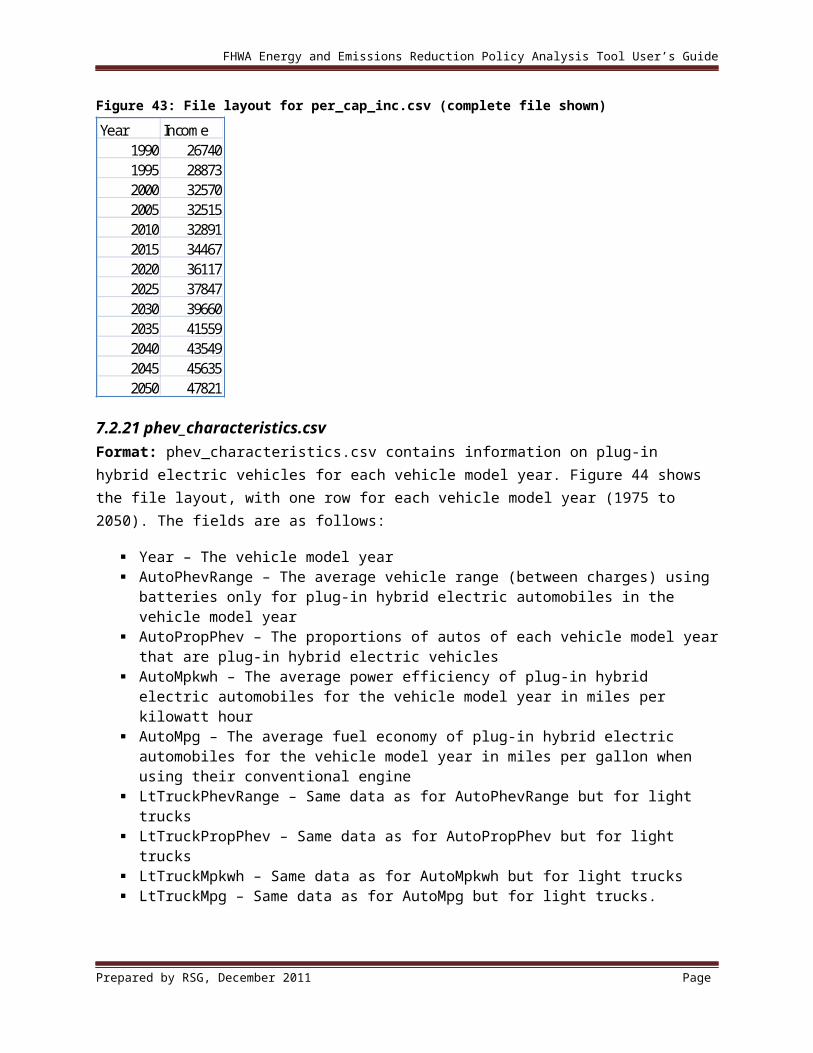
FHWA Energy and Emissions Reduction Policy Analysis Tool User’s Guide
10 ANALYSIS OF RESULTS
The FHWA tool produces large amounts of output from each model run, which can be analyzed in many ways. This section of the user’s guide describes how the output data are organized and explains conceptually how to conduct analysis of the output.
10.1 Organization of outputs
Once a run of the FHWA tool is complete, the outputs directory in the scenario folder will be populated. The outputs directory contains a directory for each forecast year for which the model was run.
In each year directory there are files containing the household simulation results for each county. These files are simply named with the name of the county and an “.RData” extension. Within each of the county files is a table called “SynPop” which contains 54 variables for each household in the county. The variables describe the household, the area it lives in, the vehicles it owns, its participation in various TDM programs, and its daily travel, fuel use, and emissions.
There is also a set of files that contain data at a more aggregate level. Most of the files are tabulations by metropolitan area for calculations that take place at that level of detail. The files created are as follows:
ArtLnMiCap.Ma.Rdata: Arterial lane miles per capita by metropolitan area AveSpeed.MaTy.Rdata: Average speeds by vehicle type (light vehicles, trucks, and buses) and
by metropolitan area BusCo2e.Ma.Rdata: Bus CO2 equivalent emissions by metropolitan area BusFuel.MaFt.Rdata: Bus fuel use by fuel type and by metropolitan area BusRevMi.Ma.Rdata: Bus revenue miles by metropolitan area DelayVehHr.MaTy.Rdata: Hours of delay by vehicle type and by metropolitan area Dvmt.CoDt.Rdata: Daily VMT by county and by development type (metropolitan, town, rural) FfVehHr.MaTy.Rdata: Hours of free flow travel by vehicle type and by metropolitan area FwyLnMiCap.Ma.Rdata: Freeway lane miles per capita by metropolitan area HhMpgAdj.Ma.Rdata: Household fuel economy adjustment by metropolitan area Inc.CoDt.Rdata: Income by county and by development type MpgAdj.MaTy.Rdata: Fuel economy adjustment by vehicle type and by metropolitan area Pop.CoDt.Rdata: Population by county and by development type RailCo2e.Ma.Rdata: Rail CO2 equivalent emissions by metropolitan area RailPower.Ma.Rdata: Rail power use by metropolitan area RailRevMi.Ma.Rdata: Rail revenue miles by metropolitan area TranRevMiCap.Ma.Rdata: Transit revenue miles per capita by metropolitan area TruckCo2e.Ma.Rdata: Truck CO2 equivalent emissions by metropolitan area TruckFuel.MaFt.Rdata: Truck fuel use by fuel type and by metropolitan area VehHr.MaTy.Rdata: Total hours of travel (free flow plus delay) by vehicle type and by
metropolitan area.
The “Year2005” directory of the base scenario also contains a file named “Pop.CoDt.RData” which is a tabulation of base year population by county and development type.
Prepared by RSG, December 2011 Page

FHWA Energy and Emissions Reduction Policy Analysis Tool User’s Guide
10.2 Analysis concepts
The FHWA tool is designed to test scenarios using a consistent framework. Therefore, the main type of analysis that users are likely to perform is to compare the results from different scenarios cross-sectionally, e.g. in 2050, how much CO2 is emitted? Other types of analysis include across years within the same scenario, and with validation datasets to compare specific outputs or series of outputs.
For household-level variables, county-level totals can be obtained by summing across all of the records in each county file. State-level totals would then be the total of the county totals. For example, summing “FuelGallons” gives total fuel used by households in a county. For complete State-level totals for aggregate variables such as VMT, fuel and power used, and emissions, the household totals must be combined with the metropolitan totals from trucks and transit.
Prepared by RSG, December 2011 Page

FHWA Energy and Emissions Reduction Policy Analysis Tool User’s Guide
11 INTEGRATION WITH MOVES
EPA's Office of Transportation and Air Quality (OTAQ) has developed the MOtor Vehicle Emission Simulator (MOVES). The MOVES website is http://www.epa.gov/otaq/models/moves/index.htm. MOVES is a new emission modeling system that estimates emissions for mobile sources covering a broad range of pollutants and allows multiple scale analysis. MOVES currently estimates emissions from cars, trucks, and motorcycles. Section 1 discusses situations when it is appropriate to use the FHWA tool instead of MOVES.
This section of the user’s guide includes:
1. A discussion of using MOVES inputs and parameters in the FHWA tool
2. An overview of how the FHWA tool can be used to generate some of the inputs that are required by MOVES (so that the emissions calculations are carried out in MOVES using its detailed emissions rates)
3. Some considerations for ensuring consistency when using the FHWA tool for preliminary scenario testing and MOVES for more detailed plan, project, and program analysis.
11.1 Using MOVES inputs and parameters in the FHWA tool
Earlier sections of this user’s guide discussed several input files to the FHWA tool that can be developed using data that have already been developed and input to MOVES. The following list provides links to those paragraphs for easy reference. Where a MOVES model exists in a State and the FHWA tool is being implemented, it is recommended that users take the following inputs from MOVES to ensure that the results obtained from each model are as consistent as possible. This is particularly important when the FHWA tool is being used for preliminary policy screening and MOVES for more detailed modeling. Consistency considerations are discussed further below.
GreenSTEP_ .Rdata – The vehicle age distributions for autos and light trucks in VehProp_, and for trucks and buses in TruckBusAgeDist.AgTy can be developed using the MOVES vehicle age distribution (SourceTypeAgeDistribution). For better consistency with MOVES, users can update the relationship between speed and fuel economy for autos and light trucks in CongModel_.
auto_lighttruck_fuel.csv – MOVES uses fuel supply, fuel formulation, and engine fuel type inputs (FuelSupply, Fuel Formulation, and FuelEngFraction) that can be used to derive the simpler fuel inputs used in the FHWA tool.
auto_lighttruck_mpg.csv – MOVES emissions inventory results can be used to calculate an average fuel economy by vehicle type and model year.
bus_fuels.csv – MOVES uses fuel supply, fuel formulation, and engine fuel type inputs (FuelSupply, Fuel Formulation, and FuelEngFraction), which can be used to derive the simpler fuel inputs used in the FHWA tool.
fuel_co2.csv – MOVES calculates “pump-to-wheels” CO2 equivalent emissions, which is consistent with the FHWA tool. However, the estimate used in the FHWA tool of the portion of CO2 equivalent emissions that comes from sources other than CO2 (i.e. CH4, N2O, and HFCs) is an
Prepared by RSG, December 2011 Page

FHWA Energy and Emissions Reduction Policy Analysis Tool User’s Guide
approximation and can be calculated in more detail using MOVES (The rates used in the FHWA tool are CO2 equivalent emissions by fuel type in grams per mega Joule of fuel energy content; these could be derived from MOVES by taking the ratio of CO2 equivalent emissions and energy consumption for each fuel type.
heavy_truck_fuel.csv – MOVES uses fuel supply, fuel formulation, and engine fuel type inputs (FuelSupply, Fuel Formulation, and FuelEngFraction), which can be used to derive the simpler fuel inputs used in the FHWA tool.
hvy_veh_mpg_mpk.csv – MOVES emissions inventory results can be used to calculate an average fuel economy by vehicle type and model year.
lttruck_prop.csv – The proportion of the passenger vehicle fleet that is light trucks can be calculated from MOVES vehicle population data (SourceTypeYear) derived from local registration data.
11.2 Using the FHWA tool to generate MOVES inputs
The FHWA tool can be used to generate some of the required inputs for running MOVES at the county scale. Under this approach the FHWA tool is used to generate inputs that can typically be produced by a State or regional travel demand model such as VMT and vehicle fleet characteristics. In areas where a State or regional travel demand model does not exist, the FHWA tool can fill that gap relatively quickly, although with less detailed information. The FHWA tool also provides a consistent framework for testing a wide range of scenarios that may be difficult or impossible to test using an existing travel demand model. Once the FHWA tool has been run to prepare MOVES inputs, MOVES is used for the emissions calculations. This approach replaces the standard data and procedures used for those calculations in the FHWA tool with comparable calculations performed by MOVES.
The MOVES inputs that can be partially or completed developed using the FHWA tool are:
Source Type Population: the number of vehicles in the geographic area that is to be modeled for each vehicle or "source type". The FHWA tool has a detailed vehicle fleet model for autos and light trucks. The household level vehicle ownership and vehicle type model results (contained in the “SynPop” table in each county results file) can be summarized up to the county level to produce the numbers of vehicles for the scenario. the FHWA tool treats heavy trucks in a more aggregate manner and so does not synthesize a heavy truck fleet.
Vehicle Age Distribution: the distribution of vehicle counts by age for each calendar year and vehicle type. As with the source type population, the household-level vehicle ownership and vehicle type model results (contained in the “SynPop” table in each county results file) can be summarized up to the county level to produce an age distribution by vehicle type for the scenario. The FHWA tool uses a heavy truck age distribution as an input, which can also be used as an input to MOVES.
Vehicle Type VMT: MOVES inputs include yearly VMT by vehicle type by county. MOVES also requires fractions to apportion VMT by month, day, and hour. The FHWA tool can provide the yearly VMT totals by vehicle type and by county for autos and light trucks by summing the VMT results in the “SynPop” table in each county results file up to the county level. These results include the VMT for every auto and light truck in the vehicle fleet.
Prepared by RSG, December 2011 Page

FHWA Energy and Emissions Reduction Policy Analysis Tool User’s Guide
Average Speeds: MOVES requires speed distribution inputs. If these are available from other sources for the base scenario, the FHWA tool outputs can be used to adjust overall metropolitan area speed distributions. The “AveSpeed.MaTy.Rdata” output contains average speeds by vehicle type (light vehicle, trucks, and buses) and by metropolitan area for alternative scenarios.
11.3 Maintaining consistency between the FHWA tool and MOVES
If the FHWA tool is used as a tool to screen a large set of policy alternatives before more detailed modeling of a subset of alternatives is carried out using MOVES, consistency between inputs used in the two model systems may be an important consideration to reduce the likelihood that decisions made at the two analysis stages are inconsistent. Users who are concerned about maintaining such consistency (and who are not, for example, simply using the FHWA tool to identify the relative efficacy of alternative policy strategies in reducing greenhouse gas emissions) should take note of the following considerations:
If, during detailed modeling, the FHWA tool is still used to produce the inputs to MOVES described above and the FHWA tool was run using model inputs that were derived from MOVES (as discussed above), the screening and detailed modeling are more likely to be consistent. For example, emissions calculations will be based on the same vehicle fleets and VMT totals. Differences will be due only to the more detailed treatment in MOVES of aspects of the calculations such as time of day/time of year and speeds.
If an alternative travel demand model is used in conjunction with MOVES, then the consistency of the FHWA tool outputs and travel demand model outputs should be checked. The key outputs to test are those discussed in Section 11.2 that could be produced by the FHWA tool and used in MOVES. For example, it is possible that VMT estimates for certain policy tests will differ between the FHWA tool and an alternative travel demand model, particularly where the sensitivity of the alternative travel demand model to the policy scenario is uncertain. It is possible to calibrate the FHWA tool against travel model outputs in order to improve model consistency in this case.
Using MOVES input: As discussed above, MOVES allows users to enter data such as vehicle fleet age distribution and population, and fuel type proportions. Similar input data are used in the FHWA tool, and so consistent inputs should be used. It is recommended that inputs derived from MOVES be used in the FHWA tool to ensure that the emissions calculations are as similar as possible.
Prepared by RSG, December 2011 Page