contentsguanine.evolbio.mpg.de/homepage/wolf.pdf · introduction 3 1 introduction in most western...

Contents

1 INTRODUCTION .................................................................3

2 THEORETICAL FUNDAMENTALS..........................................9

2.1 Immunity and Cancer ........................................................ 9 2.2 The Immune Efficiency Test (IET) – A Theranostic Approach ... 9 2.3 IET Technology ................................................................10 2.4 Database Technology........................................................16 2.5 Web Interface..................................................................20 2.6 Data Mining and Knowledge Discovery in Databases..............21

2.6.1 Data Mining Algorithms ...............................................22 2.6.2 Limitations of Data Mining............................................27

3 MATERIALS AND METHODS..............................................34

3.1 Immune Efficiency Test (IET).............................................34 3.2 IET – Database (IETDB) ....................................................35 3.3 IET – Web Interface .........................................................35 3.4 Data Mining Methods ........................................................36

4 RESULTS ..........................................................................38

4.1 Immune Efficiency Test (IET).............................................38 4.2 IET Relational Database ....................................................39 4.3 IET – Web Interface .........................................................42 4.4 Data Mining.....................................................................47

4.4.1 Business understanding ...............................................48 4.4.2 Data understanding ....................................................49 4.4.3 Data pre-processing....................................................52 4.4.4 Modelling...................................................................58 4.4.5 Evaluation .................................................................60

5 DISCUSSION....................................................................62

6 BIBLIOGRAPHY................................................................65

7 APPENDIX........................................................................71

7.1 IETDB Documentation (IET_Database.info) ..........................71 7.2 Visual Programming in Clementine......................................73 7.3 Transformer.java .............................................................77 7.4 Randomiser.java ..............................................................77 7.5 RandomisationTester.java .................................................78 7.6 IET CD............................................................................78

8 GLOSSARY .......................................................................79

9 LIST OF ABBREVIATIONS.................................................81

10 LIST OF FIGURES .............................................................83

11 LIST OF TABLES ...............................................................84

Introduction

3

1 Introduction

In most western industrialised countries, cancer and cardiovascular

diseases constitute the main cause of death and assume more

importance, as life expectancy in these societies increases. As

illustrated in Figure 1, the most common and fatal cancer types affect

human internal organs, including bronchial tubes, lungs, ovaries,

mammary and prostate glands.

Figure 1 Cancer Mortality by Tissue - Leading Causes of Cancer Deaths. This figure represents age standardised cancer mortality rates in the Federal Republic of Germany (taken from http://www.dkfz-heidelberg.de (DKFZ 2003)). Lung cancer is the leading cause of death in males and breast cancer is the leading cause in females. The most common types of cancer are – with the exception of gender-specific cancer types - largely identical.

Cancer Therapy: Conventional Approaches – Conventional cancer

therapy is based on a combination of surgery, and pre- or postoperative

radiation- and chemotherapy. Chemotherapy shows significant success

in the treatment of childhood leukaemia, but for epithelial tumour types

that constitute about 80% of all tumour-related deaths, chemotherapy

neither improves the patients’ quality of life nor increases life

expectancy (Abel 1996). Most cytostatic drugs applied in chemotherapy

Introduction

4

aim to damage DNA in order to stop proliferation of cells characterised

by high cell division rates. This is the reason why cytostatic drugs

exhibit a broad range of side effects, including potential damage of liver

and heart, as well as immune suppression (Windstosser 1994).

However, the genesis of all cancer types is to some degree due to

precancerous chronic immune deficiency. Therefore, the benefit of

cytostatic drugs in cancer therapy is questionable (Schmähl 1986).

In contrast, the benefit of radiation therapy in pre- and postoperative

treatment for the reduction of highly proliferating cancer tissue is

indisputable. Nevertheless, destroying cancer tissue by radiation

promotes the release of both cancer cell components and intact cancer

cells into the blood stream. This increases the risk of metastasis

formation and primarily, detoxification and waste disposal organs, such

as kidney and liver, are affected by new tumour growth.

Recent Developments in Cancer Therapy – In order to overcome

drawbacks arising from cytostatic drugs and radiation, modern cancer

treatment optimises existing methods and introduces principles of

adjuvant and neo-adjuvant therapy as a complement or alternative to

established approaches. Adjuvant and neo-adjuvant therapy aims to

reduce postoperative tumour regrowth or to transfer the tumour from a

non-operable into an operable state (Jatzko 2005). Different methods,

such as radiation-, chemo-, and immunotherapy, are applied alone or in

combination. In particular, immunotherapy offers several promising

principles. The most common approaches are listed in Table 1.

Introduction

5

Principle Description Active immunisation Immunisation against known tumour viruses

Non-specific active immunisation

Immunisation via synthetic molecules (cytokines: INFa,b,y, IL2, TNF)

Adaptive immunotherapy Immunity transfer or tumour resistance transfer from one individual to another via in vitro cultivation of tumour-specific lymphocytes

Passive immunotherapy Treatment with monoclonal antibodies against tumour antigens

Immunodepletive therapy

Transplantation of bone marrow

Table 1 Recent Approaches in Immunotherapy (Jatzko 2005).

In particular, theranostics, a recently emerging new field that combines

therapeutics and diagnostics, introduces promising ideas to cancer

therapy (Mazumdar-Shaw 2005). Initially, concepts of theranostics were

applied to pharmaco-genomics. In 1995, a research group at Mayo

Clinic, Rochester, USA described why the childhood leukaemia drug,

Azathioprine, caused fatality in some patients, although the drug’s

efficiency was proven in most cases. It was reasoned that a missing

enzyme, TPMT (Tiopurine methyltransferase), is responsible for the

fatality observed in certain cases (Szumlanski 1995). This raises the

question of whether or not it is sufficient to design drugs from a disease

oriented perspective. A promising alternative might be to design specific

drugs for individual patients or patient subgroups based on their

genotype (individualised therapy).

Several research groups are addressing this question differently (Diaz-

Rubio 2005; Hanrahan 2005; Shen 2005). However, many recent

approaches are similar in that they utilize principles of theranostics and

pharmaco-genetics. Here, they apply modern biomolecular techniques

to investigate both, drug response and dose finding on a genomic and

proteomic level. With the publications of the first draft sequence of the

human genome in 2001 (Lander 2001; McPherson 2001; Venter 2001),

and its subsequent completion, error correction, verification and

annotation (Stein 2004), modern medical research possesses a powerful

and vast knowledge base to support cancer research and therapy. In

Introduction

6

order to deploy this information for the benefit of gaining deeper insight

into the mechanisms and the aetiology of human diseases, it is essential

to compare genomic information with other information about human

diversity and cellular pathways. For that reason, efficient techniques

need to be applied in order to extract genomic, proteomic or

transcriptomic information, derived from messenger RNA (mRNA)

splicing, translational and post-translational variations, epigenetics

(histone code, DNA methylation etc.), protein sequence and structure,

and protein-protein interactions. High-throughput technologies with the

capability to rapidly characterise genomic functionality, constitute the

basis of functional genomics (Bailey 2002). The information gathered

via diverse techniques, including DNA sequencing, PCR, rtPCR and

qPCR, DNA and protein microarrays, native chromatin immuno

precipitation (NChIP), fluorescent in situ hybridisation (FISH), yeast two

hybrid, mass spectrometry and many more (Ideker 2001), needs to be

assembled. For that reason, powerful bioinformatics tools have been

designed to help mine biological information, and make meaningful

associations with clinical data. Hence, the combination of biological and

clinical information collated via bioinformatics is critical for deriving

near-term benefits in clinical research from the underlying basic

biomolecular knowledge.

For instance, in 1997, the Food and Drug Administration (FDA)

approved FISH technology for prenatal diagnosis (Tepperberg 2001). In

breast, bladder and renal cancer, several microarray technologies were

applied to rapidly identify associated genes, accelerate diagnosis and

adjust therapy (Man 2004). However, the main objectives of theranostic

approaches are to increase patients’ life expectancy and quality of life,

exclude ineffective or harmful medication by individually analysing the

patient’s drug and dosage response in vitro and therefore reducing

hospital and medication expenses.

Introduction

7

The Immune Efficiency Test (IET): A Theranostic Approach For Cancer

Therapy – The IET was developed and first introduced by Dipl. -Ing.

Hans-Albert Schöttler, specialist in general medicine, in 1999 and has

been applied to more than 80 patients since then. The analytical part of

the IET was performed in collaboration with Davids Biotechnologie

GmbH in Regensburg. The test is an in vitro method analysing the

ability of the patient’s immune system to kill cancer cells under the

influence of different drugs. Here the motivation is, to select the drugs

which perform best in the in vitro test and design an individualised

treatment. Most interestingly, the IET may also lead to accurate

prediction of ideal medication, which is discussed in this paper.

The immune efficiency test combines personal diagnosis with

individualised therapy and is therefore classified as theranostic

approach.

Organising and Model Building of IET data – Medication prediction

constitutes the central motivation of this IET-based study. Here,

principles of theranostics and individualised therapy are combined with

modern molecular biology and bioinformatics. This study covers the

following four tasks.

(1) Documentation of the immune efficiency test.

(2) Design and implementation of a database to store and

maintain IET data and supplemental patient information.

(3) Development and introduction of a web interface to

provide local and remote access to the database.

(4) Knowledge extraction of IET data to test the hypothesis

that predictive models estimating medication effects can

be built.

The genesis of cancer is associated with immune suppression.

Therefore, the fundamental idea of IET is that cancer therapy should

improve immune activity. For this purpose, two properties are

examined, namely the patients’ general immunological constitution and

Introduction

8

their individual ability to eliminate cancer cells. As a result, IET is a

personalised analytical assay mimicking the interacting system of

cancer and immune cells under varied medication on an in vitro

platform.

Consequently, the purpose of this thesis is to provide a detailed

documentation of the immune efficiency test, which has not been

published yet. Furthermore, the infrastructure for organising and

analysing IET data, which was designed and implemented within this

thesis, is described. In addition, this document proposes two prediction

models derived from two different machine learning algorithms, and

describes all required dataset and attribute operations in detail.

Theoretical Fundamentals

9

2 Theoretical Fundamentals

2.1 Immunity and Cancer

All types of immune cells arise from bone marrow stem cells. Some

develop into myeloid progenitor cells while others become lymphoid

progenitor cells.

Myeloid progenitor cells develop into cells that respond early and non-

specifically to infections. These include neutrophils, monocytes,

macrophages, eosinophils and basophils.

Lymphoid progenitor cells develop into lymphocytes characterised by a

later but more specific response to infections. After antigen-presenting

by dendritic cells or macrophages, lymphocytes trigger a specifically

tailored attack. Lymphocytes further differentiate into B cells, T cells,

dendritic cells and natural killer cells.

When normal cells turn into cancer cells, some surface proteins

(antigens) change. Cancer cells, like most cells, constantly release

protein fragments into the circulatory system. Tumour antigens among

these fragments prompt an immunological reaction by activating natural

killer cells and T cells. These cells provide a constant and body-wide

surveillance and eliminate cells that undergo malignant transformations.

Tumours develop when this surveillance breaks down or is overwhelmed

(NCI 2005). For this reason, lymphocyte stimulation might support this

surveillance and become a promising therapeutic option in cancer

therapy (Dunn 2005).

2.2 The Immune Efficiency Test (IET) – A Theranostic Approach

As noted in Chapter 1, theranostics (personalised medicine) is the

convergence of therapeutics and diagnostics. This neologism defines a

diagnostic tests that can identify which drugs are most suited for a

patient. Theranostic tools can provide physicians with information that


10

enables them to individualise and optimise a patient’s therapeutic

regimen (www.oralcancerfoundation.org 2004).

Immunotherapy in cancer treatment substantially necessitates the

implementation of theranostics. The ability of the immune system to

mount a response to disease is highly patient-individual and depends on

interactions between the various components of the immune system

and the antigens. The complexity of the immune system is reflected in

the presence of approximately 200 different blood group substances.

Blood groups are classified according to immunological (antigenic)

properties and are placed within 19 known blood group systems, such

as Lewis, Lutheran and MNSs. The most commonly used blood group

system is the ABO system and the association of blood group

substances to cancer is well reported (D'Adamo 2000; Madjd 2005;

Schneider 2005).

The immune efficiency test (IET) is a theranostic approach supporting

individual immunotherapy for cancer patients. The test individually

analyses the lymphocytes’ ability to detect and eliminate cancer cells

under the influence of varied therapeutic substances. This results in a

schema identifying drugs reducing or increasing lymphocytic immune

response and consequently affecting cancer growth. This schema can be

applied for individualised cancer therapy.

2.3 IET Technology

The IET probes the effect of various drugs on the interaction between

cancer cells and human lymphocytes. On the one hand, particular drugs

may directly affect cancer cells either by introducing toxic or growth

inhibitory substances. Conversely, medication may affect the human

immune system and promote immune suppression or enhancement.

The IET mimics this interactive system on an in vitro platform by

incubating lymphocytes and cancer cells, along with the drugs in

question (Figure 2).


11

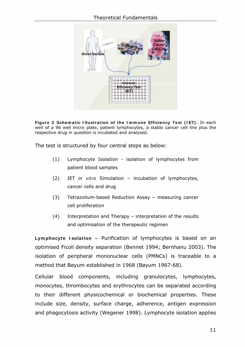
Figure 2 Schematic Illustration of the Immune Efficiency Test (IET). In each well of a 96 well micro plate, patient lymphocytes, a stable cancer cell line plus the respective drug in question is incubated and analysed.

The test is structured by four central steps as below:

(1) Lymphocyte Isolation - isolation of lymphocytes from

patient blood samples

(2) IET in vitro Simulation – incubation of lymphocytes,

cancer cells and drug

(3) Tetrazolium-based Reduction Assay – measuring cancer

cell proliferation

(4) Interpretation and Therapy – interpretation of the results

and optimisation of the therapeutic regimen

Lymphocyte Isolation – Purification of lymphocytes is based on an

optimised Ficoll density separation (Bennet 1994; Bernhanu 2003). The

isolation of peripheral mononuclear cells (PMNCs) is traceable to a

method that Bøyum established in 1968 (Bøyum 1967-68).

Cellular blood components, including granulocytes, lymphocytes,

monocytes, thrombocytes and erythrocytes can be separated according

to their different physicochemical or biochemical properties. These

include size, density, surface charge, adherence, antigen expression

and phagocytosis activity (Wegener 1998). Lymphocyte isolation applies


12

density gradient centrifugation loosely based on the Meselson and Stahl

protocol (Meselson 1958) originally developed for the investigation of

DNA replication. This method separates cells of different size and

density via centrifugation. Ficoll (specific weight: 1.077 g/ml) is a water

soluble synthetic high molecular weight (Mw = 400000 g/mol) polymer

based on sucrose and epichlorohydrin. While erythrocytes and

granulocytes pass the gradient during centrifugation (800g, 15 min)

due to their higher specific weight, lymphocytes, monocytes and

thrombocytes stay above the gradient and the lymphocyte enriched

section of the inter phase can manually be separated from the rest. The

lymphocytes isolated can then be used for further investigations.

IET in vitro Simulation – Each single IET experiment simulates the

interacting system of an immunological reaction. In this study, the

immunological in vivo system is mimicked on a micro plate platform.

Here the concept of a micro array of cells serves as a model for IET

technology. The transfer from the micro plate to a micro array platform

is intended for the near future.

In 2001, Ziauddin and Sabatini described a high-throughput tool for the

analysis of gene over-expression called “transfected cell microarray”

(Ziauddin 2001). Furthermore, cell microarray technology is applied to

siRNA (small interfering RNA) analysis (Kumar 2003; Mousses 2003)

and is integrated in several projects, including initiatives by the

Mammalian Gene Collection (MGC) (Straussberg 1999) and the Harvard

Institute of Proteomics. This aims to determine potential targets for

human diseases. The principle of a high-throughput cell microarray, as

Xu and colleges presented in 2002, serves as a model for the

technology applied in this study (Xu 2002).

The IET determines the lymphocytes’ ability to eliminate cancer cells

under the influence of various therapeutic substances by monitoring

alterations of the proliferation rate of cancer cells. In order to

successfully mimic the in vivo system, lymphocyte concentration of the

assay and of the blood sample need to be identical. The principle of


13

identical in vivo and in vitro conditions applies to the medication

conditions as well.

Tetrazolium-based Reduction Assay – Measurement of cell proliferation

and cell viability forms the general basis for many in vitro assays of a

cell population’s response to external factors. The proliferation rate of

the cancer cell line used in IET analysis is determined via a tetrazolium-

based reduction assay. This assay is based on the ability of

metabolically active cells to reduce tetrazolium salts to formazan (Aziz

2005). After 3-4 hours of incubation, formazan crystallises in early

apoptotic and living cells. By adding organic solvent, cell lysis is induced

and the crystal structure of formazan dissolves. Formazan solution

absorbs light at a specific wavelength. Cancer cell proliferation depends

on lymphocyte activity and medication. For that reason, absorbance is a

measure for cancer cell proliferation and provides a means to determine

individual patient response to a particular drug.

Interpretation and Therapy – As previously explained, the IET

simulates the immunological reaction of lymphocytes on an in vitro

platform. This gives information about 1) the patient’s individual

immunological condition and 2) the effect of a particular drug on the

lymphocytes’ ability to eliminate cancer cells. The first is assessed by

monitoring the patient-specific lymphocyte concentration in the blood

sample. The latter is probed by performing both standard reactions

without drug addition and test reactions with drug addition on the same

micro plate. The proliferation values of test and standard reactions are

normalised by the proliferation value of cancer cells without any

lymphocyte and drug addition. Therefore, all proliferation values –

measured as optical densities (ODs) – represent relative changes of the

proliferation when cancer cells alone are compared to treated cells (see

Equation 1).


14

( ) ( )Drug Control STD Control

Control Control

OD OD OD ODILA LA SPR

OD OD− −

= − = −

ILA : Induced Lymphocyte Activity

LA : Lymphocyte Activity (normalised)

SPR : Standard Proliferation Rate (normalised)

ODDrug : Optical Density of the Test Reactions

ODControl : Optical Density of the Control Reaction

ODSTD : Optical Density of the Standard Reaction

Equation 1 Calculation of Induced Lymphocyte Activities (ILA). ILA values are derived by 1) comparing and then normalising optical densities (ODs) of test and standard reactions by the OD of the control reaction and 2) subtracting the normalised standard values (SPR) from the normalised test values (LA).

The proliferation rates of the standard reactions represent the patients’

own ability to eliminate cancer cells without the aid of drug addition.

These values are henceforth called Standard Proliferation Rates (SPR,

see Equation 1 and Figure 3). The effect of a particular drug on the

lymphocytes’ ability to eliminate cancer cells is assessed by determining

the proliferation rate of cancer cells under the influence of varied drugs

when lymphocytes are present. The normalised values of these

reactions are called Lymphocyte Activity (LA). LA subtracted by the

SPR, represents the pure contribution of the drug to cancer cell

elimination/stimulation (some drugs may also stimulate cancer

proliferation). These values are called Induced Lymphocyte Activity

(ILA). The terminology of lymphocyte activity and respectively induced

lymphocyte activity refers to the fact that 1) the ability of lymphocytes

to eliminate cancer cells can also be interpreted as lymphocyte activity

and 2) medication can induce an increase or decrease in lymphocyte

activity.


15

IET Results

-17%

22%

-42%

3%

-14%

39%

-25%

20%

3%

-50% -40% -30% -20% -10% 0% 10% 20% 30% 40%

Induced Lymphocyte Activity (ILA) Lymphocyte Activity (LA) Drug 56

Drug 55

Drug …

Drug 2

Drug 1

Standard Proliferation Rate (SPR)

Lymphocyte Activity

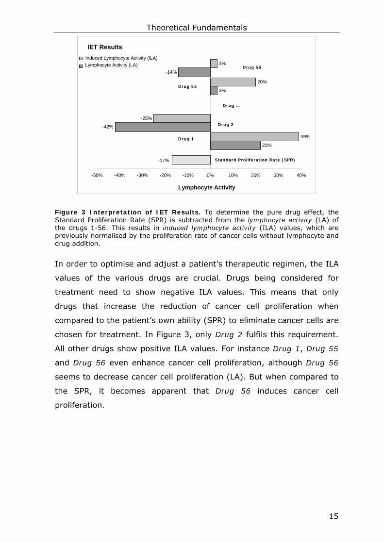
Figure 3 Interpretation of IET Results. To determine the pure drug effect, the Standard Proliferation Rate (SPR) is subtracted from the lymphocyte activity (LA) of the drugs 1-56. This results in induced lymphocyte activity (ILA) values, which are previously normalised by the proliferation rate of cancer cells without lymphocyte and drug addition.

In order to optimise and adjust a patient’s therapeutic regimen, the ILA

values of the various drugs are crucial. Drugs being considered for

treatment need to show negative ILA values. This means that only

drugs that increase the reduction of cancer cell proliferation when

compared to the patient’s own ability (SPR) to eliminate cancer cells are

chosen for treatment. In Figure 3, only Drug 2 fulfils this requirement.

All other drugs show positive ILA values. For instance Drug 1, Drug 55

and Drug 56 even enhance cancer cell proliferation, although Drug 56

seems to decrease cancer cell proliferation (LA). But when compared to

the SPR, it becomes apparent that Drug 56 induces cancer cell

proliferation.


16

2.4 Database Technology

Motivation – The history of database systems goes back to libraries,

governmental, business and medical records. There is a long tradition of

information storage, indexing and retrieving. Basically two different

approaches of information management systems are distinguished,

namely file-based systems and database systems (Connolly 2001). A

file-based system constitutes a collection of application programs

performing services for the end user. Each of these programs defines

and manages its own data. Limitations of this file-based approach are

summarised in Figure 4.

Figure 4 Turning Limitations into Innovations. Database systems turned limitations of file-based systems into innovations and are now the most commonly used data repository systems.

To overcome and prevent these limitations of file-based systems, the

database approach arose (Figure 4). Here, data is no longer simply

embedded in application programs but stored separately and

independently. This implies access and manipulation of data beyond

that imposed by application programs. A database is a shared collection

of logically related data, designed to meet the information needs of an

organisation. Here, a system catalogue provides metadata to enable


17

independence of program data. A software system that enables users to

create, define and maintain databases, and which provides controlled

access to this database, is called a database management system

(DBMS). Three types of DBMSs are as follows: hierarchical and

network-based DBMSs (first generation), relational DMBSs (second

generation) and object-relational or object-oriented DBMSs (third

generation). There are hundreds of DBMSs on the market such as MS

Acess, MS SQL server, MySQL, Oracle, Postgre SQL and many more.

Drawbacks of DBMSs are mainly due to a higher degree of complexity,

which is accomplished by the demands of trained users. Nevertheless,

the advantages of DBMSs significantly exceed the drawbacks as

illustrated in Figure 4 and are therefore used for information storage in

this study.

Relational Database Model – The relational model was developed from

the work done by E. F. Codd in the late 1960s (Sol 1998) and now

constitutes the most commonly used database model. The fundamental

structure of the relational model is the concept of tables (also called

relations) in which all data is stored. Each table constitutes of records

(horizontal rows, also called tuples) and fields (vertical columns, also

called attributes) and is identified by a unique key attribute (primary

key). This key is essential for the DBMS to organise and find records.

This distinguishes the relational model significantly from hierarchical or

network-based models, in which the user is responsible for data

structure within the database. Querying of relational databases is

simply done by comparing the value stored within a particular column

and row to some criteria. Users can query information concerning table

names, access rights, storage types etc. This simplifies administration

of the database, as well as usage.


18

Database Design Methodology – The database design methodology is a

structured approach using procedures, techniques, tools and

documentation aids to support and facilitate the process of design.

Database design is structured as follows:

(1) Conceptual Database Design – Conceptual database

design is the process of constructing a model of

information used in an enterprise, independent of all

physical considerations. Here, the “real-world” domain is

specified and captured. All entity and relationship types

are identified and associated with the respective

attribute types. This is done by using a database design

model (Entity-Relationship-Model – E/R model (Chen

1976)).

(2) Logical Database Design – Transformation of a

conceptual model into local and global logical data

models supported by the DBMS (Relational Model (Sol

1998)). Normalisation procedures ensure that

information will be non-redundant and properly

connected.

(3) Physical Database Design – The relational model is

translated into tasks physically concerning the DBMS.

Here, the implementation of the database is described

including file organisation, indexing, user views, security

mechanisms and analysis of disk space requirements,

among others.

Separation of database design into these three phases reduces the

complexity of database projects. If not all design decisions depend

mutually on one another, problems can be separated and solved one

after the other. In order to increase the efficiency of a database,

normalisation is performed (logical database design). This is the process

of increasing efficiency of a database by eliminating redundant

information and assessing significance of data dependencies by a set of


19

rules. Most commonly four different normal forms are distinguished and

defined as follows (Kennedy 2000).

• Un-normalised Form (UNF) – A table that contains

one or more repeating groups.

• First Normal Form (1NF) – A relation in which

intersection of each row and column contains one and

only one value.

• Second Normal Form (2NF) – A relation that is in 1NF

and every non-primary-key attribute is fully functionally

dependent on any candidate key.

• Third Normal Form (3NF) – A relation that is in 1NF

and 2NF and in which no non-primary-key attribute is

transitively dependent on any candidate key.

• Boyce-Codd Normal Form (BCNF) – A relation that is

in 3NF and all determinants are candidate keys.

In practice, the boundaries of the three design phases are overlapping

and even de-normalisation is a common means to introduce a different

logical model for performance purposes (Angus 2001). In addition,

adjustments or alterations of the physical design (software and/or

hardware) may be required to meet performance requirements. This

can easily be done, if database design was conducted in separate

phases. In general, separation of database design into these three

phases increases flexibility and simplifies implementation of large

database projects.


20

2.5 Web Interface

For the interaction of a client with a data repository system, several

approaches including mainframe and two tier architecture are available.

However, the most commonly used client-server architecture is three

tier client-server architecture (also known as multi tier architecture,

Figure 5). The first tier (client) contains the presentation logic, including

simple control and user input validation. The second tier (application

server), provides the business logic and data access. Tier three

(database server), provides the business data.

This architecture enables easy modification and replacement of one tier

without affecting the others. Additional, separating application and

database functionalities enhances load balancing and security policies

can be enforced within the server tiers without interfering with the

client (Ramirez 2000).

First TrierClient

Second TierApplication

Server

Third TierDatabase Server

Tasks- User Interface- Presentation logic

Tasks- Business logic- Data processing logic

Tasks- Business Data- Data validation- Database access

Figure 5 Three-Tier Client Server Architecture. This architecture separates the three domains Client, Application Server and Database Server.

Most web applications accessing a database directly via a browser (web

interface) use three tier client-server architecture. For communication

of DBMSs with the Web, several approaches are available. Along with


21

Common Gateway Interface (CGI) technology, the use of scripting

languages (JavaScript, VBScript, Perl and PHP) extending browser and

web server with database functionality are the most common

techniques.

The world wide web (www) constitutes the most popular and powerful

networked information system to date. The www was designed to be

platform-independent and therefore, web-based applications can

significantly lower deployment and implementation costs. Web sites

today contain more and more dynamic information. The content of a

dynamic Web page is generated each time it is accessed. This enables

the web page to respond to user input and to provide customised views.

However, accessing a database via the web (Web-DBMS Approach)

involves some drawbacks, primarily those concerning reliability and

security. Nevertheless, the Web-DBMS approach is a simple and

platform-independent application to access a database via the Web.

2.6 Data Mining and Knowledge Discovery in Databases

“Data Mining is the process of exploration and analysis, by autonomic or

semi-autonomic means, of large quantities of data in order to discover

meaningful patterns and rules.” (Johansson 2004)

Several terms have been put forth to describe the process of

discovering useful patterns in data. These include data archaeology,

data mining, data pattern processing, information discovery and

information harvesting (Fayyad 1996). The term data mining has in

particular been used by statisticians and data analysts, but it is now

also commonly used in the database field. The term knowledge

discovery in databases (KDD) emphasises the fact that knowledge is the

result of a data-driven discovery (Piatetsky-Shapiro 1991). In general,

KDD is the overall process of discovering meaningful knowledge. One

step of this process is data mining which aims to discover and extract

underlying patterns from data through the application of specific

algorithms (Brodley 1999). The central motivation of the KDD approach


22

is to transform low-level data into a more abstract, compact and useful

format. This may result in a model of the process that generated the

data, a brief report or a prediction model to estimate future values. KDD

is an iterative process comprising the following six stages.

(1) Basic Understanding of the Enterprise

(2) Dataset Creation

(3) Correction or Removal of Corrupted Data

(4) Data Reduction

(5) Model Building by the Use of Data Mining Algorithms

(6) Interpretation and Validation of the Results

These operations are summarised in CRISP-DM 1.0 (Chapman 1999) a

widely accepted methodology to design and describe the KDD process.

2.6.1 Data Mining Algorithms Data mining is an AI-powered procedure that aims to discover

meaningful information from a data source that then can be used to

improve action. To achieve this objective data mining uses machine

learning algorithms. Machine learning refers to a process or system

capable of autonomously acquiring and integrating knowledge (AAAI

2006). Both machine learning and data mining are subtopics of AI. In

2004, John McCarthy defined intelligence as the “…computational part

of the ability to achieve goals in the world. Varying kinds and degrees of

intelligence occur in people, many animals and some machines…”

(McCarthy 2004). This is a general – even so anthropological –

definition of intelligence and enables us to explain the term AI. The

American Association for Artificial Intelligence describes AI as “…the

scientific understanding of the mechanisms underlying thought and

intelligent behaviour and their embodiment in machines…” (Reddy

1996). The technical implementation of AI results in the development of

algorithms, such as flexible rule interpreters, artificial neural networks

(ANNs) and self organising software (Sloman 1998).


23

AI-powered algorithms are implemented in several data mining

software tools which most commonly provide unsupervised (grouping

into similar, initially undetermined classes) and/or supervised

(predictions using already determined classes) machine learning

algorithms (Mangasarian 1990; Mangasarian 1990; Wolberg 1990;

Bennet 1992). Both types – supervised and unsupervised – are

implemented in Clementine (SPPS) providing implementations of Build

C5.0, classification and regression tree (CART), ANN and Kohonen

algorithms. However, many other comparable software tools are

available, such as Darwin (Thinking machines, Corp.), Intelligent Miner

(IBM), CART (Salford Systems) (Elder 1998)

Several prediction methods have been published using machine learning

in gene expression profiling (Golub 1999; Brown 2000; Furey 2000).

These studies demonstrate the substantial demand of restricting

prediction models by taking account of the competing demands of

simplicity and accuracy (Brazam 2000). This principle applies to

immune efficiency profiling as well. Therefore, this study focuses on the

application of the two supervised machine learning algorithms ANN and

CART as described by Dudoit (Dudoit 2002). The algorithms are

discussed below.

Artificial Neural Networks (ANNs) – ANN algorithms simulate neuronal

information processing of the human brain at a very basal level. ANNs –

as their human paradigm – are able to learn and generate expert

abilities on a trial and error basis. Table 2 summarises and Figure 6

illustrates analogies between artificial and biological neural networks.

Biological Neural Network Artificial Neural Network Soma Neuron Dendrite Input Axon Output Synapse Weight

Table 2 Analogy between Biological and Artificial Neural Networks.

Learning of ANNs is performed with a large number of single subunits

(neurons) organised in different layers (usually input-, middle- and

output-layer). The linkage of these subunits is implemented by variable


24

connection weights (Figure 6). Based on the investigation of several

individual data points, an ANN formulates predictions for each single

record and adjusts the previously defined connection weight in case the

prediction was incorrect. The definition of stopping criteria enables the

user to terminate this self-repeating process (SPSS 1994-2003).

Neurons constitute the central processing units of an ANN and are

organised as illustrated in Figure 6. A neuron receives several weighted

input signals, computes a new activation function and sends the result

to its output link. For instance, the output is “–1” if the weighted sum of

the input signals is less than a certain threshold. If the input is higher

than the threshold, the neuron becomes activated and the output

attains “+1”. This particular activation function is called sign function.

However, several other activation schemes have been tested, including

step, linear and sigmoid functions (Negnevitsky 2002). Depending on

the activation function chosen and the resulting output signal, the input

weights are updated differently. This process is performed iteratively.

A

B

C

Figure 6 Architecture of Biological and Artificial Neural Networks. Section A) depicts a biological neural network, B) the basic architecture of an artificial neural network and C) illustrates a single neuron of an artificial neural network.


25

In conclusion, the training process of ANNs is performed in four steps:

(1) Initialisation – The initial weights (w1, w2,…,wn), a

certain threshold and the activation function are defined.

(2) Activation – The neuron output is calculated based on

the activation function chosen and the respective

weighted input.

(3) Weight training – The input weights are updated

according to the difference between the respective

output and the expected value.

(4) Iteration – Iteration starts at step 2 and is repeated

until convergence.

Classification and Regression Tree (CART) – CART is a decision tree

algorithm and “…takes as input an object or situation described by a set

of properties, and outputs a yes/no decision…” (Russell 1995). Decision

making of CART algorithms is therefore based on Boolean functions.

CART is a predictive rule induction algorithm that estimates future

values by using binary recursive partitioning. The original records are

split into fragments of similar output values. These partitions are ranked

in order to find the best fragment. This process proceeds until a

stopping criteria is reached. Most commonly, CART uses the Gini

coefficient1 as criterion to drive splitting (Luan 2002; Ranawana 2006),

but also the tree-depth is a means of defining the termination of

recursion. In general, rule induction algorithms cull through a set of

predictors by successively splitting the data set of choice into subsets

based on interactions of predictor and output fields. Recursive splitting

results in the construction of decision trees (Sessum 2001).

Figure 7 illustrates a four layer decision tree generated by using a CART

algorithm and built upon data derived from the breast cancer database

established at the University of Wisconsin Hospitals (Madison, USA) by

1 The Gini coefficient is a dispersion measure to analyse any form of uneven distribution. This statistical measure was developed by the Italian statistician Corrado Gini and his paper “Variabilità e mutabilità” was published in 1912 (http://en.wikipedia.org/wiki/Gini_index).


26

Dr. William H. Wolberg (Mangasarian 1990; Mangasarian 1990; Wolberg

1990; Bennet 1992). Based on cellular properties, the tree predicts a

binary class label holding the values “2” (benign) and “4” (malignant)

with an accuracy of ~96%. The tree shows that the Uniformity of Cell

Shape attribute is most significant for predicting the class label. For

94% of the patients being considered “benign”, the Uniformity of Cell

Shape attribute is characterised by a value lower than 3.5. Conversely,

87% of the patients being considered “malignant” show values of higher

than 3.5. This reflects the binary nature of the CART algorithms.

Figure 7 Decision Tree Built by Applying a CART Algorithm. The data are derived from the breast cancer database established at the University of Wisconsin, Madison. Each instance has one of two possible classes: “2” for benign and “4” for malignant. All other attributes are discrete numeric attributes with a range from “1” to “10”, where “1” indicates that the attribute can not be applied to the respective instance and “10” that it can be fully applied.

Conclusion. While CART algorithms are easy to train, represented

visually by trees and therefore provide interpretable models of the

underlying data sets, ANNs are usually characterised by a faster

response and lower computational times, but lack explanation facilities


27

and act as a black box. They essentially are models without information

concerning the internal components or algorithms of the storage device

(Wang 2004).

2.6.2 Limitations of Data Mining While data mining is a significant advance of the analytical tools

currently available to analyse large data sets, they are not self-

sufficient applications and there are limitations to their capability

(Seifert 2004).

Although data mining can aid in revealing patterns and relationships, it

does not assess the significance of these patterns in a causal sense.

This type of determinations can not be automated in data mining and

must be performed by analytical personnel. The validity of the patterns

depends on how well “real world” situations are explained. Data mining

can identify connections and different connection weights between

variables and the patterns discovered might describe the real world

situation accurately but it does not necessarily increase the knowledge

about the nature of the problem and how it is caused (Seifert 2004).

For successful data mining, skilled analytical personnel is required to

structure the analysis, interpret the output and formulate meaningful

results. Consequently, personnel or data limitations do primarily affect

the success of data mining, rather than technical constraints.


28

In this chapter, four different techniques are described to overcome

some of the aforementioned limitations.

(1) CRoss Industry Standard Process for Data Mining

(CRISP-DM) – to structure data mining projects.

(2) Hypothesis Testing for Statistical Dependencies –

to detect potential patterns before modelling algorithms

are applied.

(3) Validation by a Training and Validation Set Splits –

to investigate how patterns discovered compare to

unknown circumstances.

(4) Randomisation Testing – to assess significance of

patterns discovered.

CRISP-DM – CRISP-DM methodology was published by NCR Systems

Engineering Copenhagen, DaimlerChrysler AG, SPSS Inc. and OHRA

Verzekeringen en Bank Groep B.V in 1999 (Chapman 1999). It

combines an industry proven guideline for data mining projects with

helpful advices for proper documentation of the process and for clean

presentation of the results.

In CRISP-DM methodology, the terminology slightly differs from the

initially mentioned KDD process. In CRISP-DM, the term data mining

refers to the entire process of knowledge discovery and the actual data

mining phase, as defined above, is called modelling or model building.

Nevertheless, CRISP-DM methodology constitutes the most commonly

used standard protocol for knowledge discovery.

CRISP-DM methodology is best displayed as a life cycle model (shown in

Figure 8). The model includes six phases, business understanding, data

understanding, data preparation, modelling, evaluation and

deployment, with arrows indicating the most important dependencies.

The sequence of the phases is not strict and allows the analyst to go

back and forth as needed. This guarantees flexibility for the users’

diverse needs.


29

Business Understanding

Data understanding

Data preparation

Modelling

Evaluation

Deployment

Data

Figure 8 Phases of the CRISP-DM Reference Model. CRISP-DM includes the following six phases: business understanding, data understanding, data pre-processing, modelling, evaluation and deployment. (Chapman 1999)

The surrounding outer circle in Figure 8 refers to the cyclical nature of a

data mining project and emphasises that a data mining lifecycle does

not necessarily terminate, once one turn is finished. In most cases,

deployment solutions trigger new questions for the previous phases

such as business- or data understanding.

The initial phase of business understanding guides the analyst of a data

mining project from a basic understanding of the diverse requirements

and objectives to a first problem definition and a design of preliminary

concepts for solving the problem from a business-oriented perspective.

Data understanding entails the intensive investigation of the initial

dataset in order to assess data quality and to become aware of the type

and format of information. Moreover, this process provides a first

insight into the dataset and promotes the discovery of interesting

subsets, first hypotheses and/or constraints. Without the use of

machine learning algorithms, data understanding explores the dataset

on a basal level and feeds into data pre-processing. Main tasks concern

dataset, data and attribute considerations.


30

In-depth data understanding enables the analyst to proceed with data

pre-processing, which covers activities such as assortment of significant

records, attributes and subsets while disposing irrelevant information.

Furthermore, in many cases data transformation and formatting is

required to construct a dataset compatible with the modelling

algorithms of choice. In cases of high-dimensional feature space, data

pre-processing needs to be performed in two steps: First, pure data

preparation, including data formatting, integrating, selecting, cleaning

and constructing tasks; Second, a feature selection phase, to reduce

feature space dimensionality (Piatetsky-Shapiro 2003). Here, several

approaches such as T-test for Mean Difference, Stepwise forward

selection or stepwise backward elimination are available (Han 2001).

The modelling phase applies various data mining algorithms to the

dataset and adjusts respective parameters such as pruning or stop

criteria to build significant models. Typically, different algorithms

require different data formats and consequently stepping back to the

data pre-processing phase may be required.

After successful model building, it is important to evaluate the model

before deployment. The evaluation phase reviews all actions of the

previous phases and probes whether or not the model takes all initially

defined business objectives into account. Most importantly, quality and

significance of the models generated are assessed here.

Deployment is the final phase of a data mining project which makes use

of the findings, models and documentations of the study. In most cases,

the deployment phase is not carried out by the analyst, but by the

customer.

Hypothesis Testing for Statistical Dependencies. Assuming underlying

patterns to the data given – and only then will model building be

successful – statistical dependencies within the data will be detectable

as well. By introducing hypothesis testing before model building is

performed, the success of data mining algorithms on a given dataset

can be investigated. On the one hand, this increases data mining


31

efficiency, since irrelevant datasets or subsets can be excluded and on

the other hand patterns discovered during model building are

confirmed. To prove statistical dependencies, the principle of linkage or

gametic disequilibrium can be used. Linkage disequilibrium was defined

by Brown and colleges who employed this concept to detect

associations of Hordeum Spontaneum alleles among different loci

(Brown 1980). This principle is used in LIAN 3.0 (from LInkage

ANalysis), a software tool to test the null hypothesis of linkage

equilibrium for multilocus data (Haubold 2000). LIAN was originally

used to detect linkage disequilibrium in bacterial populations (Haubold

1998), but can be applied to any multilocus data such as IET data.

Statistically relevant associations or linkage disequilibrium can be

assumed if the null hypothesis can be rejected.

Validation by Training/Validation Set Splitting. Splitting the initial

dataset into training and validation sets enables the analyst to perform

model building and validation on two separate datasets. In doing so, it

can be investigated how patterns discovered during model building

compare to unknown circumstances. This mimics a “real world”

situation. Most commonly, training and validation is performed with a

70%/30% randomly split dataset (Gansky 2003; Piatetsky-Shapiro

2003; Bloom 2004; Chakraborty 2005).

Similarly, in cases of high feature space and low number of instances,

cross-validation can be performed (Radmacher 2002).

Randomisation Testing. Validating by training/validation set splits,

however, is not sufficient for assessing the significance of a model. A

small error rate found during validation does not necessarily guarantee

that the patterns are significant (Radmacher 2002). To assess

significance, it needs to be tested whether or not the models built

perform significantly better than due to chance alone. This can be done

using randomisation testing (Manly 1991).

For instance, in this study, 1241 immune efficiency profiles were used

for model building. Five different class labels can be assigned to each


32

profile. This results in 51241 ≈ 10867 possible combinations for predicting

the outcomes of the 1241 profiles. This number is too huge for any

computer to analyse all possible permutations. Thus, a large sample

(e.g. N=105) is used to estimate the proportion of random predictions

that have an accuracy better than the model. This is done by randomly

shuffling the actual class labels (ACLs) N-times and thus generating N

randomised class label (RCL) sets (Figure 9). The percentage of RCL

sets characterised by a higher accuracy than the predicted class label

(PCL) set generated by the model is represented by the p-value. For

instance, a p-value of 0.25 indicates that 25% of the RCL sets

performed just as well as or better than the model. Therefore, the

model may not be considered as significantly describing the underlying

dataset.


33

Figure 9 Randomisation Testing. (A) depicts the initial dataset and shows the actual class labels (ACL) for four instances. Model Building (B) generates predicted class labels (PCL) based on the supplemental information (attributes A to Z). Randomisation testing (C) shuffles the ACLs N times and consequently generates N randomised class labels (RCL). Comparison of RCL to ACL results in the distribution of prediction accuracy. The p-value represents the portion of the distribution that exceeds the accuracy level achieved by model building (or the p-value is the percentage of RCL sets performing better than the PCL set).

Materials and Methods

34

3 Materials and Methods

This section summarises all materials and methods required for this

study. This includes technology to 1) perform the IET test; 2) create a

relational database to store IET results along with clinical and general

patient information; 3) implement a web-interface to access the

database and 4) build predictive models to estimate drug effects.

3.1 Immune Efficiency Test (IET)

The IET analyses the proliferation rate of a stable cancer cell line under

the influence of various drugs and patient individual lymphocytes. The

proliferation rate is a measure to determine the usefulness of particular

drugs for a specific patient. The test is performed in the following three

steps:

Lymphocyte Isolation - Based on optimised Ficoll density separation,

lymphocytes were isolated from whole blood using Ficoll-PaqueTM Plus

and following the manufacturers’ instructions (Amersham Bioscience,

Uppsala, Sweden).

IET Incubation – Cancer cells of a stable and well defined cancer cell

line (details on the cancer cell line can not be published) were incubated

at 37°C in a 96 well micro array along with the drug under review and

patient lymphocytes. The cancer cell concentration was adjusted to 106

cells per millilitre. The total volume was 200µl. Lymphocyte

concentration corresponded to the concentration in the blood sample.

Drug concentration reflected the physiological dosage of the drug.

Culture medium was Dulbecco’s Modified Eagle Medium (DMEM) with

additives.

Measurement of Cancer Cell Proliferation – Cancer cell proliferation

was measured using Mosmann’s MTT reduction assay (Mosmann 1983).

For each sample three wells of a 96-well microplate were used. 100µl of

the sample plus 10µl of MTT stock solution (5mg MTT/ml of PBS) was


35

incubated for three hours at 37°C. The absorbance was measured

subsequently using a spectrometer at the wavelength specific for

formazan absorbance.

3.2 IET – Database (IETDB)

IETDB was organised with a relational model and stored in MYSQL

4.0.23 relational database management system. The database was

implemented via phpMyAdmin (phpMyAdmin 2.6.0-rc3), a commonly

used platform for database implementation in MySQL. For database

design Microsoft Office Visio Professional 2003 was used. The SQL code

is presented on the IET CD.

3.3 IET – Web Interface

Three tier architecture was used for assessing IETDB via a web

interface. The web interface connects to the IETDB and was constructed

by HTML scripts running on an Apache/2.0.48 web server. Client

interference with the database was implemented via php-embedded

SQL statements. All logical operations were executed in php and by

JavaScript code embedded in HTML code. The source code of the web

interface can be found on the IET CD.


36

3.4 Data Mining Methods

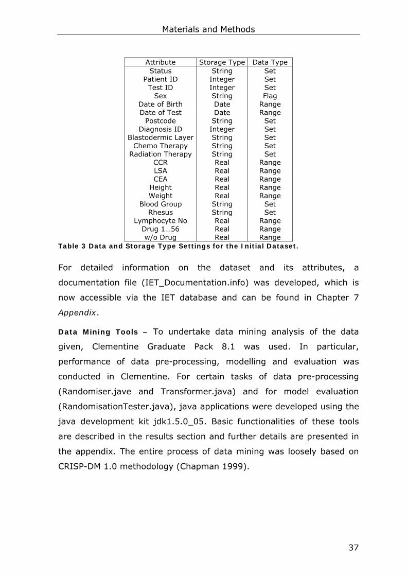
Initial Dataset – All information available from patient charts (see

Figure 10) was integrated into one dataset (Microsoft Excel format).

Figure 10 Structure and Attributes of a Patient Chart – The Basis for the Initial Dataset. The various attributes are sorted by the type of information they belong to. The three sources of information were integrated into one Excel file.

Consequently, this dataset was organised in a patient-wise manner (i.e.

each single entry hold the complete IET result – for drug1 through

drug56 – for a particular patient). Altogether, the dataset hold 105

entries for 75 attributes. Most attributes are self-explanatory, e.g. the

attribute Blastodermic Layer can take “meso” for meso dermal, “ekto”

for ekto dermal and “endo” for endo dermal. Data and storage types of

all attributes are summarised in Table 3.


37

Attribute Storage Type Data Type Status String Set

Patient ID Integer Set Test ID Integer Set

Sex String Flag Date of Birth Date Range Date of Test Date Range

Postcode String Set Diagnosis ID Integer Set

Blastodermic Layer String Set Chemo Therapy String Set

Radiation Therapy String Set CCR Real Range LSA Real Range CEA Real Range

Height Real Range Weight Real Range

Blood Group String Set Rhesus String Set

Lymphocyte No Real Range Drug 1…56 Real Range w/o Drug Real Range

Table 3 Data and Storage Type Settings for the Initial Dataset.

For detailed information on the dataset and its attributes, a

documentation file (IET_Documentation.info) was developed, which is

now accessible via the IET database and can be found in Chapter 7

Appendix.

Data Mining Tools – To undertake data mining analysis of the data

given, Clementine Graduate Pack 8.1 was used. In particular,

performance of data pre-processing, modelling and evaluation was

conducted in Clementine. For certain tasks of data pre-processing

(Randomiser.jave and Transformer.java) and for model evaluation

(RandomisationTester.java), java applications were developed using the

java development kit jdk1.5.0_05. Basic functionalities of these tools

are described in the results section and further details are presented in

the appendix. The entire process of data mining was loosely based on

CRISP-DM 1.0 methodology (Chapman 1999).

Results

38

4 Results

The aim of this study was to document the immune efficiency test and

to organise and explore IET data. At this point, more than 80 patients

have been tested, their specific immunological reaction was monitored

and based on these results an individualised therapy was applied.

Chapter 4 presents tools developed for organising and exploring IET

data. For this purpose, a relational database was created incorporating

IET, clinical and general data. To provide access to this database, a web

interface was created. Finally, based on IET and supplemental

information, knowledge discovery and data mining techniques were

applied for model building. The motivation was to clarify whether or not

models predicting medication effects can be found. This study proposes

two different prediction models of proven significance and accuracy.

4.1 Immune Efficiency Test (IET)

Depending on the patient’s anamnesis, ten to twenty different drugs are

tested per IET. The motivation of each test is to identify drugs that

positively affect the immune system and therefore promote the

reduction of cancer cell proliferation. In this study, criteria for accurate

medication were understood and mathematically described (positive

drug effects are characterised by a negative Induced Lymphocyte

Activity; see equation 1 in Theoretical Fundamentals). Drugs associated

with an increase in cancer cell proliferation are excluded from the

therapeutic regimen. At the time this study started, IET had been

applied to 82 patients. Some patients were tested more than once.

Altogether 56 different drugs had been tested resulting in more than

1200 single experiments.

Results

39

4.2 IET Relational Database

In order to store, access and update general, clinical and IET data, a

relational database was designed and implemented. Database design

was performed within the three phases conceptual, logical and physical

database design. The database was subsequently implemented on a

MYSQL 4.0.23 relational database management system.

Conceptual Database Design. The dataset given hold general and

medical patient information along with test data and results of the

respective drugs. This results in the definition of five basic entities:

Patient, Immune Efficiency Test, Laboratory Tests, Diagnosis and Drug

(illustrated in Figure 11). All attributes of the initial dataset can be

assigned to one of these entities.

Figure 11 Entity Relationship (E/R) Model. The five basic entities Patient, Immune Efficiency Test, Laboratory Tests, Drug and Diagnosis are connected as shown above. All attributes of the dataset given can be assigned to one of the four entities as illustrated.

Logical Database Design. Logical database design develops a logical

model describing the real world domain captured within the E/R model.

For this purpose, normalisation of the initial dataset was performed.

Results

40

Figure 12 Un-normalised Form (UNF) of the IET database. The UNF contained redundant information (highlighted red) that was removed during the process of normalisation.

Figure 12 reveals some of the dependencies that occurred in the

dataset given. Test information depends on patient information in a way

so that each patient can have more than one single test, but each test

requires exactly one single patient. Moreover, each patient needs to

have one single diagnosis, whereas the same diagnosis can be assigned

to more than one patient. In addition, each single drug has metadata

including a drug group and a description, but each drug group may

describe more than one drug. Therefore, redundancies occur within the

UNF. In order to transfer the UNF into 1NF all redundancies had to be

resolved.

For this purpose, separate patient and test tables along with the unique

identifiers Patient_ID and Test_ID were created. In addition, both tables

were further split in order to resolve remaining redundancies and to

integrate metadata (drug group and description). This was done by

generating Diagnosis and Drug tables. Consequently, this required a

separate IET_Results table for assessing the test results of each drug

being tested within a particular IET. IET_Results is a so-called “weak

entity”2, which is only defined by the two tables Drug and Test. After

creating the unique identifiers Diagnosis_ID and Drug_ID for the tables

Diagnosis and Drug, further investigation of these five tables revealed

that the design was also in 2NF, since no partial dependencies occurred.

2 In relational databases, a weak entity is an entity that cannot be uniquely identified by its own attributes alone (http://en.wikipedia.org/wiki/Weak_entity).

Results

41

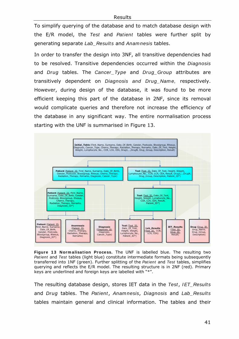
To simplify querying of the database and to match database design with

the E/R model, the Test and Patient tables were further split by

generating separate Lab_Results and Anamnesis tables.

In order to transfer the design into 3NF, all transitive dependencies had

to be resolved. Transitive dependencies occurred within the Diagnosis

and Drug tables. The Cancer_Type and Drug_Group attributes are

transitively dependent on Diagnosis and Drug_Name, respectively.

However, during design of the database, it was found to be more

efficient keeping this part of the database in 2NF, since its removal

would complicate queries and therefore not increase the efficiency of

the database in any significant way. The entire normalisation process

starting with the UNF is summarised in Figure 13.

Figure 13 Normalisation Process. The UNF is labelled blue. The resulting two Patient and Test tables (light blue) constitute intermediate formats being subsequently transferred into 1NF (green). Further splitting of the Patient and Test tables, simplifies querying and reflects the E/R model. The resulting structure is in 2NF (red). Primary keys are underlined and foreign keys are labelled with “*”.

The resulting database design, stores IET data in the Test, IET_Results

and Drug tables. The Patient, Anamnesis, Diagnosis and Lab_Results

tables maintain general and clinical information. The tables and their

Results

42

relationships are summarised in the logical model presented in Figure

14.

Figure 14 Relational Model of the IET-Database in 2NF. The relational model shows tables, relationships and attributes. The different tables are assigned to the three types of information stored within the database: general, clinical and IET information. Primary keys (PK) are underlined and ‘FK’ indicates foreign keys. The arrows indicate the direction of the dependency. For instance, Anamnesis depends on Patient.

Physical Database Design. The relational model illustrated in Figure 14

served as a logical model for physical database design. The tables of the

relational model were directly used to implement the database. All

attributes, primary and foreign keys as illustrated in Figure 14 could be

adopted to implement the database on a relational database

management system. The manageable size of the database, did not

require disk space and performance considerations so far.

4.3 IET – Web Interface

In order to maintain, update and access the database, a user-friendly

web interface was developed and connected to the IETDB using three

Tier architecture. Here, the IET-web interface constitutes the top tier

and provides user interference. The third tier provides IETDB

management functionality and is implemented using a MySQL database

Results

43

server. The middle tier provides process management services that can

be shared by multiple applications. Here, an Apache/2.0.48 web server

was employed.

This reflects the fact that the database will not only serve as a local

data repository, but might be accessed via the internet in the near

future. For this reason, a basic user management model was developed.

The web interface distinguishes between ‘read only’ and ‘read/write’

users.

The IET - web interface operates the underlying database and offers

three main functionalities for user interaction:

(1) Data Retrieval – Information stored in the database

can be displayed and optionally be downloaded.

(2) Data Insertion – New information can be incorporated

into the database.

(3) Data Editing – Information stored in the database can

be edited.

Data Retrieval – Two basically different options for data retrieval were

implemented in the IET web interface. The first involves a pure display

of information. This includes general drug and patient details, the

respective IET and laboratory results, along with information about

diagnosis and anamnesis. This option will primarily be used by medical

practitioners requiring a platform for easy and fast information retrieval,

for example details concerning a particular patient.

In addition to this display function, the interface provides a download

option to retrieve the entire database as a comma separated value

(csv) file. In addition, a documentation file for the database can be

displayed and alternatively be downloaded (IET Documentation

function). This functionality was implemented for analysts who for

example perform data mining on the database. Both functionalities are

shown in Figure 15.

Results

44

Figure 15 Data Retrieval. Two distinct modes for data retrieval were developed: a pure display of information accessible via the VIEW functions (upper red circle) and the CSV retrieval and IET Documentation (lower red circle) download options. The right frame shows the retrieval form used to access patient details.

Data Insertion – The insert option was developed for medical

practitioners and can only be accessed by read/write users. This

function supports incorporation of new drug-, diagnosis- and patient-

information along with the respective IET- and laboratory results. Figure

16 illustrates how to insert new patient information.

Figure 16 Data Insertion. Four options were developed for data insertion, namely New Patient, New Result, New Drug and New Diagnosis. Exemplarily, insertion of new patient information is displayed in the right frame.

Results

45

The New Results option operates both the insertion of new IET data and

laboratory information. New results can only be inserted if the patient

already exists within the database. Insertion of new results is performed

in two steps. First, general and clinical information is entered and the

drugs being tested are selected from a pull-down list. Second, IET

results are entered for the respective drugs. These two steps are linked

via confirmation logic implemented by embedded JavaScript code that

summarises all inputs of the first step (Figure 17). This aims to prevent

the aberrant storage of type errors into the database. Another

JavaScript pop-up window has to be confirmed before IET results are

sent to the database (this is not shown in Figure 17). All other Insert

options were linked to JavaScript confirmation logic in the same way.

1

3

2

Figure 17 Data Insertion – New Result. Insertion of new results (IET and laboratory results) is carried out in two steps. First, the insertion of general information such as Height and Lymphocyte No plus the selection of the drugs being tested (left red circle, 1). Second, the insertion of the IET results for the previously selected drugs (right red circle, 3). These two steps were linked via a JavaScript pop-up window (2) to confirm the entries of the first step. Before sending the new results to the database, another JavaScript pop-up window needs to be confirmed (not shown in Figure 17).

Results

46

Data Editing – Data editing is closely linked to data retrieval and uses

the VIEW options to select the type of information for being edited or

deleted. This functionality can only be accessed by read/write users.

The result frame of each query provides options for editing or deleting.

In case the delete record option was chosen, deletion needs to be

confirmed before the command will be executed at the database level.

The edit record option leads to another frame to change the respective

entry. The edition of the entry needs to be confirmed in a java-script

pop-up window. Figure 18 shows this sequence of forms for updating

patient information.

1

2

3

4

Figure 18 Edit Data. Editing of records is shown for patient information. After querying for a particular patient (1), the result frame (2) gives options to edit or delete the respective entry. When selecting edit record the Edit Patient Information menu (3) is started. Before updating the database with the edited version of the record, all alterations must be confirmed in a JavaScript pop-up window (4).

In conclusion, the IET web interface provides standard functionalities to

maintain and update the database, and to view and retrieve the

information stored. Since the database holds sensitive patient

information, the following three aspects of data security were

implemented:

Results

47

(1) Secure Data Transfer Protocols (SSL) – Secure

Sockets Layer (SSL) is a asymmetrical cryptographic

protocol providing secure communication and endpoint

authentication on the internet. The Apache server used

was authenticated using SSL 3.0.

(2) Validation of Potentially Insecure User Input - PHP

provides the function mysql_real_escape_string() to

escape potentially insecure user input and therefore to

avoid SQL Injections. The term SQL Injection defines a

security vulnerability occurring in the database layer of

an application by incorrect escaping of string literals

embedded in SQL.

(3) Basic Access Management – User management of the

IETDB web interface covers two different user situations:

read only users and read/write users. For both

password-protection was implemented.

4.4 Data Mining

The fundamental objective of this data mining study was to investigate

whether or not predictive models estimating future effects of particular

drugs on individual patients can be built and validated based on IET

data.

Therefore, this study had access to more than 80 immune efficiency

tests (~ 1200 single measurements). Each measurement constituted an

individual experiment investigating the ability of lymphocytes to

eliminate cancer cells under the influence of particular drugs. Here, the

proliferation rate of the cancer cells was monitored. Along with the

respective clinical and general patient information, individual immune

efficiency profiles were designed. These profiles can be used in data

mining, for instance, to discover biologically similar drugs or risk

circumstances for cancer development or to construct multivariate

predictors of group memberships. The latter is covered within this study

which proposes two models for predicting the effect of particular drugs

Results

48

on cancer patients. Here, principles of CRSIP-DM methodology

(Chapman 1999) are applied.

4.4.1 Business understanding Business Objectives. This data mining project integrated IET, general

and clinical information resulting in the generation of individual immune

efficiency profiles. The project’s objective was to clarify whether or not

prediction models for personalised medication can be developed based

on the exploration of immune efficiency profiles.

Assess situation. All resources required to achieve the business

objective were available. These included CRISP-DM 1.0 data mining

guide, Clementine Graduate Pack 8.1 and the dataset itself, which could

legally be used for this study. Recommended system requirements for

Clementine were fulfilled (Operating System: Microsoft Windows XP or

Windows 2000 Professional; Hardware: Intel Pentium compatible

processor; Memory: 512 MB RAM; Minimum free disk space: 320MB

(SPSS 2005)).

Data mining objectives. In order to implement the business objective,

the following four data mining objectives needed to be achieved.

(1) Data Integration – Combination of general, clinical and

IET data in order to design individual immune efficiency

profiles.

(2) Test for Attribute Dependency – The detection of

statistical attribute dependency that indicates underlying

patterns within the profiles and makes model building

reasonable.

(3) Model Building - Design of prediction models for

personalised medication.

(4) Quality and Significance Assessment – Validation of

the prediction models designed.

Results

49

Project Plan. The project schedule of this data mining project was

basically structured by CRISP-DM 1.0 methodology (compare Figure 8).

All data available were used for model building and validation.

Therefore, no data could be placed at the disposal of a deployment

phase. For this reason, the deployment phase was excluded, although

all other considerations of CRISP-DM were implemented in this project.

4.4.2 Data understanding Data understanding results in advice and considerations that need to be

conducted in the data pre-processing phase. Here, we can divide the

considerations found into three categories, namely Dataset, Data and

Attribute considerations.

Dataset Considerations – As a requirement of the third data mining

objective (pp. 47), the class attribute of the dataset needs to be a

measure representing the effect of particular drugs. In the initial

dataset, this demand was fulfilled by the attributes Drug1 to Drug57. In

order to design prediction models for medication based on IET data, one

single class attribute (Actual Class Label, ACL) is required. A statistical

model predicts the ACL by generating Predicted Class Labels (PCL). For

that reason, the initial dataset needs to be transformed from a patient-

wise into a drug-wise format. This implies the substitution of the

patient-oriented attributes Drug1 to Drug57 by one drug-oriented class

attribute representing drug effects and one additional attribute

identifying the respective drug.

For model building and validation, the initial dataset needs to be divided

into a training set and a validation set. To guarantee compatibility to all

modelling algorithms of potential interest, the dataset needs to be

formatted.

Data Considerations – In most cases, more than one test was

performed per patient. Results of the test were used to adjust

medication. However, information about these adjustments was not

Results

50

available. For this reason, only the first test of each patient can be

included, since subsequent tests do not guarantee independence.

Moreover, a detailed data quality report is required to assess if it is

necessary to remove other records.

Attribute Considerations – Generally, attribute operations may increase

knowledge and spur the achievement of data mining goals. In the given

dataset, some of the drugs can be grouped based on their chemical,

structural or functional properties. Therefore, it is reasonable to

introduce a new attribute called Drug Group.

Moreover, the combination of attributes may increase the information

content. In our case, the two attributes Date of Test and Date of Birth

should be merged to the more meaningful attribute, Age at Test. The

attributes Height and Weight should be linked to the attribute BMI

(body mass index).

In addition, exclusion of attributes might be a useful means to increase

the accuracy of prediction models. All attributes originating from

database design, including Test ID and Patient ID can be excluded.

Moreover, the attribute Postcode is of no relevance within this study.

However, the importance of attributes can hardly be predicted before

applying modelling algorithms to the dataset. Nevertheless, the impact

of the attributes Blood Group and Rhesus to cancer was analysed more

closely, since their influence in cancer is already well-reported

(Dabelsteen 2005; Madjd 2005; Schneider 2005; Yei 2005). Several

publications associate blood group effects with breast carcinoma, oral or

gastric cancer (Dabelsteen 2005; Madjd 2005; Yei 2005). Moreover, in

2005, Schneider et al proved the significant impact of the rhesus factor

on the development of symptomatic meningioma and found that rhesus

positive cases were less frequent in the underlying patient group

(Schneider 2005). Basal analyses of the IET dataset showed strong

interactions of blood group A and status malignant (60.66%, Figure

19).

Results

51

Figure 19 Web Graphs of the Attributes Blood Group, Rhesus and Status. Strong interactions were shown for blood group A, malignant and unknown rhesus factor (left graph, strong interactions are labelled bold). When focusing on the attributes Blood Group and Status (right graph) the correlation between blood group A and the malignant state became more evident. No conclusion could be drawn from interactions between blood group AB and the malignant state, since blood group AB is only represented by one single record. Significant associations between blood group 0 and either malignant (27.27%) or benign (24.59%) were not found.

Since blood group AB was only represented by one single record,

associations of blood group AB could not be taken into account. The

attribute Rhesus may be removed from the dataset due to its high

number of missing values (69.51%).

In conclusion, strong associations were only found between blood group

A and the malignant state, whereas blood group 0 and B were

characterised by indifferent interactions. Consequently, the attribute

Blood Group needs to be included in this study. No associations of the

attribute Rhesus were found due to low data quality. This shows the

need for general attribute quality verification.

Results

52

Conclusions. In Table 4, all suggestions and considerations obtained

from the Data understanding phase are summarised for being

transformed into operations within the subsequent data pre-processing

phase.

Dataset Considerations

Data Considerations

Attribute Considerations

Dataset Transformation:

Transform the dataset from a patient-wise into a drug-wise format; this includes some attribute operations.

Series Exclusion:

Exclude test series by only selecting the first test of each patient; this guarantees independence.

Grouping:

Group the various drugs by introducing the new attribute, Drug Group.

Formatting:

Before starting model building, the final dataset needs to be formatted to guarantee compatibility with modelling algorithms.

Data Quality Analysis:

Decide whether or not particular entries should be excluded.

Combination:

Combine the following attributes: Date of Test/Date of Birth to Age at Test and Weight/Height to BMI.

Sampling:

Generation of training and validation subsets for evaluation.

Exclusion:

Analyse attribute quality and relevance.

Table 4 Advices and Consideration Acquired from Data Exploration.

4.4.3 Data pre-processing In this study, data pre-processing was mainly concerned with the

integration of general, clinical and proliferation information. This

provided a suitable dataset of individual immune efficiency profiles for

data mining. All considerations derived from the data understanding

phase were transformed into operations and finally aided in obtaining

reliable prediction models for the data.

Results

53

Dataset Operations

Dataset Transformation. To perform the transformation from a patient-

wise into a drug-wise format, a java application (Transformer.java) was

developed. Functionality of this application is illustrated in Figure 20.

Figure 20 Dataset Transformation from Patient-wise to Drug-wise Format. This operation was performed by the java application Transformer.java.

Here, the initial attributes Drug 1 to Drug 56 were substituted by the

two attributes Result and Drug ID. The attribute w/o Drug got the

Drug_ID “0”. All other drug IDs (e.g. “3”) represented the initial

attribute name (e.g. Drug 3). This guaranteed unique identification of

each particular proliferation measurement and defined the single class

attribute Result. In doing so, the number of attributes decreased from

75 to 22 while the number of instances increased from 106 to 1241.

Sampling. Another java application (RandomDistributor.java) was

developed to generate random subsets of the initial dataset. These

subsets were required for training and validation of prediction models.

The training set hold ~70% (871 instances) and the validation set

~30% (370 instances) of the initial dataset. Here, it was crucial to

guarantee that the two datasets did not overlap and that the validation

set was not used in any way for model building.

Results

54

Data Operations

Series Exclusion. Only the first test of each patient was taken for

further investigation. Exclusion of the remaining entries was performed

within the original excel file before transferring the dataset into

Clementine.

Data Quality Analysis. In Clementine, a Quality node was used to

assess data quality. Missing values needed to be declared in Clementine

but did not affect further modelling. This was done by using a Type

node.

Attribute Operations

Grouping. Most drugs could be grouped according to their physical,

biological or chemical properties as shown in Table 5. For that reason, a

new attribute Drug Group was included, without substituting the

attribute Drug ID. This operation was also implemented in MS Excel by

using basic if/else expressions.

Table 5 Grouping of Drug ID According to Chemical or Structural properties. This table lists all drug subgroups and their respective candidates. Due to data security, the actual drug can not be published yet. Please note that Drug ID “0” represents the control reactions and is listed as a separate group.

Combination. In this study, the attributes Date of Birth and Date of Test

were less important than the age of a particular patient. Therefore,

Date of Birth and Date of Test were merged to a new attribute called

Age. The attributes Height and Weight were combined in the same way

by introducing a new attribute called BMI (body mass index). This

reduced feature space and simplified the initial dataset without affecting

the amount of information. This operation was undertaken in

Clementine.

Group Drug ID Description Group 0 0 Control Group 1 37, 41, 50, 56 Enzyme Group 2 13, 18, 22, 25, 26 Mistletoe Group 3 32, 33, 47, 48, 49 Thymus Group 4 30, 54, 55 Vitamin Group 5 All others Others

Results

55

Exclusion. Criteria for data selection include relevance of information for

the data mining objectives and data quality. As discussed before, the

attributes Postcode, Patient ID and Test ID did not contribute to

knowledge discovery and were therefore omitted. The 17 remaining

attributes, were analysed in terms of data quality. This included two

tasks. First, the declaration of all user defined missing values and

second, the quality analysis and exclusion of attributes characterised by

low data quality. Missing values have already been declared in Data

Operations. Results of the data quality analysis are listed below. Both

data quality analysis and attribute exclusion were performed by using a

Quality node which excludes values of quality lower than 50% by

default. Table 6 shows data quality of the various attributes and

indicates those being excluded for further investigations in bold.

Attribute % complete Number of Legal values

Status 92.1 1143 Sex 100.0 1241 Age 94.2 1169

Diagnosis 92.1 1143 BlastELSEmic layer 92.1 1143

Chemo Therapy 39.24 487 Radiation Therapy 39.24 487

CCR 10.64 132 LSA 5.48 68 CEA 6.77 84 BMI 100.0 1241

Blood Group 99.03 1229 Rhesus 33.36 414

Lymphocyte No. 100.0 1241 Drug ID 100.0 1241

Drug Group 100.0 1241 Result 100.0 1241

Table 6 Data Quality Report. Completion rate and the number of legal values are provided for each attribute. Attributes being excluded after assessing data quality are labelled in bold.

Results

56

Format Data

To guarantee compatibility with the modelling algorithms used, the

dataset needed to be formatted. Most machine learning algorithms

require discrete class labels. This demanded the introduction of the new

class attribute Effect based on the former class attribute Result. All

Result values were assigned to one of the following subsets: high

increase, increase, stagnancy, reduction and high reduction of the

proliferation rate. Identification of the various subsets was done by

applying a scheme of even numbers ‘0’, ’2’, ’4’, ’6’, ’8’ as summarised in

Table 7.

Change of Proliferation rate [%]

Effect Explanation

-10 to 10 0 Stagnancy 10 to 50 2 Increase

-10 to -50 4 Reduction 50 to 100 6 High Increase

-50 to -100 8 High Reduction Table 7 Relationship of the Proliferation Rate and the New Class Attribute Effect. Based on the change of the proliferation rate (-100% to 100%), the new class attribute Effect was designed. Here, a scheme of even numbers was applied, but other schemes may serve equally.

Here, reduction of the proliferation rate indicated effectiveness of the

respective drug, since proliferation of the cancer cell line was reduced.

In turn, Increase signalled an ineffective drug, since the growth of the

cancer cell line was up-regulated.

Most commonly, numeric variables are required for analysis. Therefore,

the storage type of all string attributes was transformed to numeric.

This affects the Status, Sex, Blastodermic Layer, Diagnosis and Blood

Group attributes. These string attributes were transformed by a scheme

of even numbers as listed in Figure 21.

Results

57

CLASS

Not known 0Malignant 2Benign 4

SEX

F 2M 4

F – femaleM - male

Blastodermic Layer

Not known 0Meso 2Ekto 4Endo 6Control 8

Bloodgroup

Not known 0A 2B 4AB 60 8

Diagnosis

Not known 1Bronchial Ca. 2Colon Ca. 3Control 4Esophagus Ca. 5Glioma 6Intestinal Ca. 7Leukemia 8Maignant Melanoma 9Mamma Ca. 10Myosarcoma 11Nasopharynx Ca. 12Ovarian Ca. 13Pancreas Ca. 14Prostata Ca. 15Rectum Ca. 16Renal Ca. 17Sigma Ca. 18Squanous Epithelium Ca. 19Stomach Cancer 20Uterus Ca. 21Vaginal Ca. 22Vesica Ca. 23Immune Deficiency 24

Figure 21 Compilation of String and Numeric Values of the Respective Attributes. Attributes of the storage type string were transformed into numeric values. Figure 21 shows the initial string value in contrast to the new numeric value.

Please note that cases of immune deficiency (ID 24) were treated

separately from control cases, although both attributes are classified as

benign. Cancer patients frequently show immune deficiency as well and

therefore it is essential to distinguish between these cases. Otherwise

discrimination of control and cancer cases may decrease significantly.

In conclusion, the sequence of operations described above produced

two datasets (training and validation set) of 11 attributes holding 1241

records altogether. Table 8 summarises the attributes being used for

modelling, reports completion rates and lists the range of values, as

well as storage and data types.

Results

58

Attribute % complete Storage Type Data Type Value Age 94.2 Real Range [22.5, 91.4]

Blastodermic layer 92.1 Integer Set 0*, 2, 4, 6, 8 Blood Group 99.03 Integer Set 0*, 2, 4, 6, 8

BMI 100.0 Real Range [16.7, 36.7] Diagnosis ID 92.1 Integer Set 1,…,24 Drug Group 100.0 Integer Set 0, 1, 2, 3, 4, 5

Drug ID 100.0 Integer Set 0,…,56 Lymphocyte No. 100.0 1Real Range [0.31, 4.5]

Sex 100.0 Integer Flag 2, 4 Status 92.1 Integer Set 0*, 2, 4 Effect 100.0 Integer Set 0, 2, 4, 6, 8

Table 8 Final Attribute Properties. Completion rates, the range of values, as well as data and storage types are listed for each of the 11 attributes of the final dataset. The class attribute Effect is in bold. Values labelled with * constitute user defined missing values and once declared, they do not appear in Clementine any more.

The dimensionality of the feature space was reduced from 75 to 11.

Most importantly, the dataset was transformed into a drug-wise format

integrating clinical, general and proliferation information. The

combination of these different sources of information resulted in

individual immune efficiency profiles, which can be used for testing

whether or not prediction models for the class attribute Effect can be

built.

4.4.4 Modelling In order to answer the question whether or not prediction models based

on immune efficiency profiles can be built, four tasks were to be

executed.

(1) Hypothesis Testing for Statistical Dependencies

(2) Determine Settings for Class Prediction

(3) Selection of the Prediction Method

(4) Model Building

Hypothesis Testing for Statistical Dependencies. Prior to starting the

model building process, it was essential to probe whether or not

statistical dependencies of the attributes can be found. In the case of

statistical dependency, we can assume underlying patterns within the

Results

59

dataset. It is only then that further investigations to determine

prediction models become reasonable.

For this exercise, LIAN 3.0 (Haubold 1998; Haubold 2000) was used.

Analyses of the dataset using LIAN showed highly significant

associations between attributes (P =10-4) and therefore gave reason to

suspect patterns associated with the dataset. Based on this finding,

modelling algorithms were applied to the dataset to build meaningful

prediction models.

Settings for Class Prediction. This study aimed to produce prediction

models for the declared class attribute Effect. For this reason,

supervised algorithms were most useful for model building.

Selection of a Prediction Method. In this study, a prediction method

loosely based on Dudoit and colleges (Dudoit 2002) was applied by

employing the two modelling algorithms ANN and CART.

Model Building. C&R tree, a CART version of Clementine, and an ANN

approach were applied for model building. The C&R tree algorithm

(using default settings with a maximum tree depth of 10) applied to the

training dataset, identified the attributes Diagnosis ID and Lymphocyte

No as most important for class prediction. The ANN algorithm using

default settings without the prevention of overtraining, defined the

attributes Blood Group, Blastodermic Layer, Age and Lymphocyte No as

most important. These attributes are characterised by their similar

relative importance (0.19, 0.18, 0,14 and 0.13).

Results

60

4.4.5 Evaluation Regardless of the prediction method chosen, in order to assess the

quality and significance of the models, it was necessary to perform

validation and randomisation testing, asking the question “if the models

perform well on the training set, will they also predict the class attribute

accurately when applied on unknown data?”

When testing the two models on the validation set, the C&R tree model

achieved an accuracy of 63.0%. In 61.1% of the cases, the ANN model

predicted the class attribute correctly. These findings showed that the

two algorithms can be used to build predictive models estimating the

effect of a specific drug, based on immune efficiency profiles. However,

significance of the models has not yet been proven. For that reason,

randomisation testing was performed. This task was conducted by

developing a java application (RandomisationTesting.java).

Randomisation testing showed that correct class prediction by chance

alone obtained a mean accuracy of 34% (Figure 22) and a p-value of

1x10-5 when compared to the two prediction models.

Std.Dev = 0.02Mean = 0.34N = 10,000

0

0,05

0,1

0,15

0,2

0,25

0,3

0,35

0,4

0,22 0,24 0,26 0,28 0,3 0,32 0,34 0,36 0,38 0,4 0,42 0,44 0,46 0,48

Prediction Accuracy [%]

Perf

orm

ance

Figure 22 Randomisation Test. Distribution of prediction accuracy produced by N = 10,000 randomly generated predictions.

This evidence definitely reveals the significance of the previously

designed models.

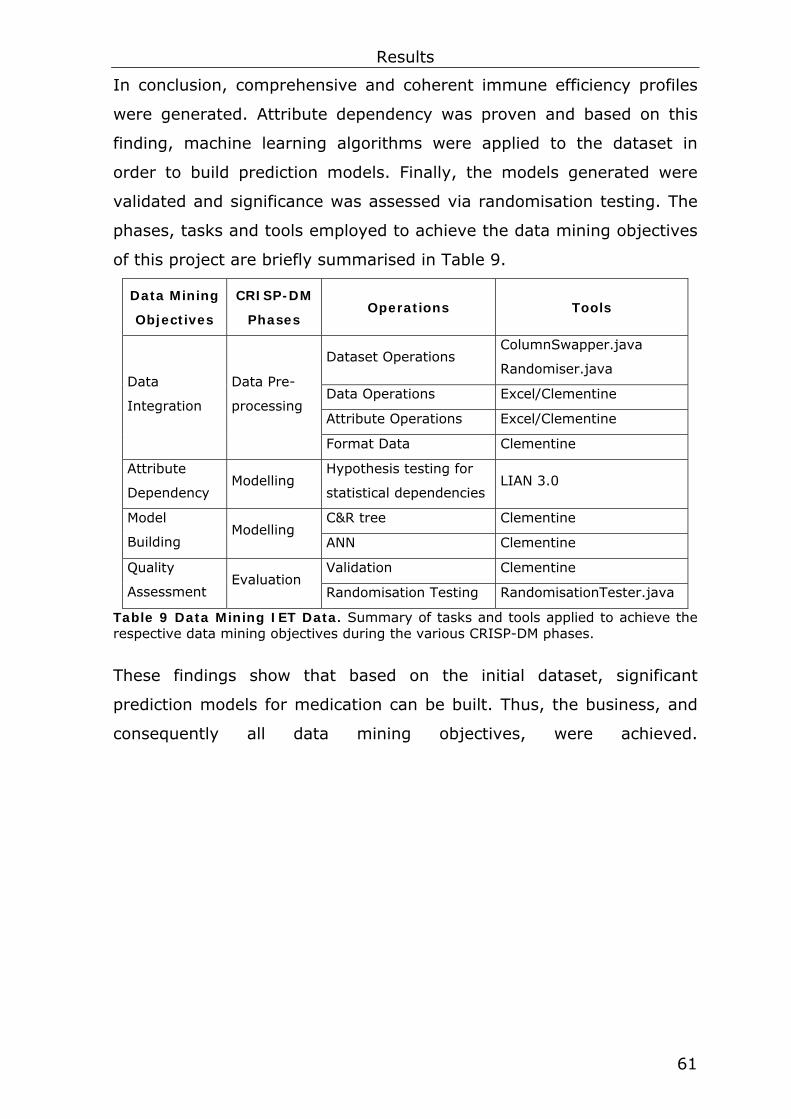
Results

61

In conclusion, comprehensive and coherent immune efficiency profiles

were generated. Attribute dependency was proven and based on this

finding, machine learning algorithms were applied to the dataset in

order to build prediction models. Finally, the models generated were

validated and significance was assessed via randomisation testing. The

phases, tasks and tools employed to achieve the data mining objectives

of this project are briefly summarised in Table 9.

Data Mining

Objectives

CRISP-DM

Phases Operations Tools

Dataset Operations ColumnSwapper.java

Randomiser.java

Data Operations Excel/Clementine

Attribute Operations Excel/Clementine

Data

Integration

Data Pre-

processing

Format Data Clementine

Attribute

Dependency Modelling

Hypothesis testing for

statistical dependencies LIAN 3.0

C&R tree Clementine Model

Building Modelling

ANN Clementine

Validation Clementine Quality

Assessment Evaluation

Randomisation Testing RandomisationTester.java

Table 9 Data Mining IET Data. Summary of tasks and tools applied to achieve the respective data mining objectives during the various CRISP-DM phases.

These findings show that based on the initial dataset, significant

prediction models for medication can be built. Thus, the business, and

consequently all data mining objectives, were achieved.

Discussion

62

5 Discussion

Immune Efficiency Test – The main focus of conventional cancer

therapy including chemo- and radiation therapy is to maximise tumour

eradication within the limits of tolerable toxicity and radiation to the

organism. Recently, several approaches arose to overcome or assist

such conventional therapy. These include adjuvant and neo-adjuvant

therapy, immunotherapy and theranostic approaches. Within the field of

theranostics, the immune efficiency test (IET) presented in this study

provides a novel approach of individualising cancer therapy as an

alternative or supplement to conventional therapy. The IET combines

immunotherapy with theranostics and enables the medical practitioner

to selectively compare different treatment strategies and to optimise

the patients’ therapeutic regimen based on these findings.

Storage and Maintenance of IET data – This thesis presents techniques

required to store and maintain IET data, along with supplemental

patient information including general and clinical data. For this purpose,

a relational database was created. To access this data, a web interface

was implemented and connected to the database. The database

efficiently represents the “real world” domain. However, future

alterations concerning the IET and/or supplemental information may

require adjustments of the database. Similarly, alterations of the web

interface may also be required once the system is deployed and tested.

This study identified and implemented two different user types – read

only users and read/write users. This results in a clearly defined

permission management for accessing the functionalities for data

retrieval, data editing and deletion. This is sufficient to effectively

access and maintain the current database. However, database growth

and accessibility of the database via the Web and/or a local network,

may require adjustments of user management, functionalities and

security aspects.

Discussion

63

Analysis of IET data – In 1999, Shochat and colleges presented a

computational approach using “…computer simulations for evaluating

the efficacy of breast cancer chemotherapy protocols” (Shochat 1999).

Schochat modelled the effect of chemotherapy on tumour mass and

simulated the outcome of several treatment protocols. The ensuing

mathematical models have been used to design treatment protocols and

to identify patterns among the many combinations of drug dosage and

scheduling. Their work showed that computer sciences may enhance

medical research and help to individualise therapy. In recent years,

several other research groups demonstrated the utility of the concept of

computer aided medical research and therapy. In 2005, Arakelyan et al.

validated a computer model for predicting tumour growth based on data

obtained by dynamic measurements of tumour growth and

vascularisation dynamics (Arakelyan 2005). In addition, computer

modelling has been used to simulate anaphylactic reactions due to

chemotherapeutic reactions (Castiglione 2003) and to understand the

complex process of angiogenesis – the formation of new blood vessels

(Arakelyan 2003) – which has a widespread significance in cancer

therapy (Folkman 1995; Folkman 2005).

Within this context, this thesis combines the concept of theranostics in

immunotherapy with computer science. This study proves that the

modelling of IET data provides predictive models estimating the effect

of a treatment strategy. Here, two models were built that significantly

predict the patient specific induced lymphocyte activity range (ILA-

range) of various drugs based on supplemental patient information. To

prove this concept, the machine-learning algorithms ANN and CART

were used and the models derived were validated via training/validation

set splitting and randomisation testing. Consequently, the objective was

neither to optimise the models built nor to compare different machine

learning algorithms. Nevertheless, in order to apply these models for

treatment, the prediction accuracy of 63.0% (CART) and 61.1% (ANN)

respectively is not sufficient and needs to be optimised. This can be

Discussion

64

achieved, by adjusting the algorithms, increasing sample size and/or

employing other algorithms.

In conclusion, this study not only proved the concept of computer

simulations for the prediction of therapeutic regimens, but also

proposed a general framework for analysing IET data. This framework

includes crucial steps as data pre-processing for creating individual

immune efficiency profiles, model building and evaluation of predictive

models, and can be applied to all future studies analysing IET data.

Bibliography

65

6 Bibliography

AAAI (2006). Machine Learning. AI Topics. http://www.aaai.org, Menlo Park, USA, American Association for Artificial Intelligence.

Abel, U. (1996). Die zytostatische Chemotherapie fortgeschrittener epithelialer Tumoren - eine kritische Bestandsaufnahme. Stuttgart, Hippokrates.

Angus, V. (2001). Database Review - Database Design Guidelines. http://www.abdn.ac.uk/clsm/dbase, Aberdeen, UK, Institute of Applied Health Sciences, University of Aberdeen: 1-12.

Arakelyan, L. (2003). Multi-Scale Analysis of Angiogenic Dynamics and Therapy. Cancer Modelling and Simulation. L. Preziosi. Torino, Italy, Chapman & Hall/CRC.

Arakelyan, L. (2005). "Vessel maturation effects on tumour growth: validation of a computer model in implanted human ovarian carcinoma spheroids." European Journal of Cancer 41: 159-167.

Aziz, D., M. (2005). "Application of MTT reduction assay to evaluate equine sperm viability." Theriogenology 64: 1350-1356.

Bailey, S., N. (2002). "Applications of transfected cell micro-arrays in high-throughput drug discovery." Drug Discovery Today 7: 1-6.

Bennet, K., P. (1992). Robust linear programming discrimination of two linearly inseparable sets. Optimization Methods and Software 1, Gordon and Breach Science Publisher.

Bennet, S. (1994). "Variables in the isolation and culture of human monocytes that are of particular relevance to studies of HIV." Journal of Leukocyte Biology 56: 236-240.

Bernhanu, D. (2003). "Optimized lymphocyte isolation methods for analysis of chemokine receptor expression." Journal of Immunological Methods 279: 199-207.

Bloom, G. (2004). "Short Communication - Multi-Platform, Multi-Site, Microarray-Based Human Tumor Classification." American Journal of Pathology 164: 9-16.

Bøyum, A. (1967-68). "Isolation of mononuclear cells and granulocytes from human blood." Scandinavian Journal of Clinical and Laboratory Investigations 21-22: 77-89.

Brazam, A. (2000). "Gene expression data analysis." FEBS Letters 480: 17-24.

Brodley, C., E. (1999). "Knowledge Discovery and Data Mining." American Scientist 87: 54.

Brown, A., H., D. (1980). "Multilocus structure of natural populations of Hordeum spontaneum." Genetics 96: 523-536.

Bibliography

66

Brown, M., P., S. (2000). "Knowledge-based analysis of microarray gene expression data by using support vector machines." Proceedings of the National Acadamy of Sciences, USA 97: 262-267.

Castiglione, F. (2003). The effect of drug schedule on hypersensitive reactions: a study with a cellular automata model of the immune system. Cancer Modelling and Simulation. L. Preziosi, CRC Press.

Chakraborty, S. (2005). "Bayesian neural networks for bivariate binary data: An application to prostate cancer study." Statistics in Medicine 24: 3645-3662.

Chapman, P. (1999). CRISP-DM 1.0, Step-by-Step data mining guide, NCR System Engineering Copenhagen, Daimler Crysler AG, SPSS INC., OHRA Verzecheringen en Bank Groep B.V.

Chen, P. (1976). "The Entity-Relational Model- Toward a Unified View of Data." ACM Transactions on Database Systems 1: 9-36.

Connolly, T. a. B., C. (2001). Database Systems: A Practical Approach to Design, Implementation, and Managemanet. Boston, Addison Wesley Higher Education.

Dabelsteen, E. (2005). "ABO blood-group antigens in oral cancer." Journal of Dental Research 84: 21-8.

D'Adamo, P., J. (2000). ABO Blood Group and Cancer, www.dadamo.com.

Diaz-Rubio, G., E. (2005). "A panel discussion of controversies and challenges in the adjuvant treatment of colon cancer." Clinical and Translational Oncology 7: 3-11.

DKFZ (2003). The 20 Most Frequent Causes of Cancer Deaths 2003. http://www.dkfz-heidelberg.de, Heidelberg, Deutsches Krebsforschungszentrum.

Dudoit, S. (2002). "Comparison of discrimination methods for the classification of tumors using gene expression data." Journal of the American Statistic Association 78: 316-331.

Dunn, G. (2005). "Dendriti cells and HNSCC: A potential treatment option? (Review)." Oncology Reports 13: 3-10.

Elder, J., F. (1998). A Comparison of Leading Data Mining Tools. Fourth International Conference on Knowledge Discovery & Data Mining, New York, New York, Elder Research.

Fayyad, U. (1996). "From Data Mining to Knowledge Discovery in Databases." AI Magazine Fall 1996: 37-54.

Folkman, J. (1995). "Angiogenesis in cancer, vascular, rheumatoid and other diseases." Nature Med 1: 27.

Folkman, J. (2005). "Antiangiogenesis in cancer therapy - endostatin and its mechanims of action." Experimental Cell Research 312: 594-607.

Bibliography

67

Furey, T., S. (2000). "Support vector machine classification and validation of cancer tissue samples using microarray exression data." Bioinformatics 16: 906-914.

Gansky, S., A. (2003). "Dental Data Mining: Potential Pitfalls and Practical Issues." Advances in Dental Research 17: 109-114.

Golub, T., R. (1999). "Molecular classification of cancer: Class discovery and class predicition by gene exression profiling." Science 286: 531-537.

Han, J. (2001). Data Mining: Concepts and Techniques. San Francisco, California, Morgan Kaufmann Publishers.

Hanrahan, E., O. (2005). "Neoadjuvant systemic therapy for breast cancer: an overview and review of recent clinical trials." Expert Opinion on Biological Therapy 6: 1477-1491.

Haubold, B. (1998). "Detecting linkage disequilibrium in bacterial populations." Genetics 150: 1341-1348.

Haubold, B. (2000). "LIAN 3.0: detecting linkage disequilibrium in multilocus data." Bioinformatics Application Note 16: 847-848.

Ideker, T. (2001). "Integrated genomic and proteomic analysis of a systematically perturbed metabolic network." Science 292: 929-934.

Jatzko, G. (2005). Kolorektales Karzinom. http://www.aco.at, Austrian Society of Surgical Oncology.

Johansson, U. (2004). Accuracy vs. Comprehensibility in Data Mining Models. The 7th International Conference on Information Fusion, Stockholm, Sweden, International Society of Information Fusion.

Kennedy, D. (2000). Database Design and the Reality of Normalisation. Proceedings of the NACCQ 200, Wellington, NZ.

Kumar, R. (2003). "High-throughput selection of effective RNAi probes for gene silencing." Genome Research 13: 2333-2340.

Lander, E. S. (2001). "Initial sequencing and analysis of the human genome." Nature 409: 860-921.

Luan, J. (2002). "Data Minig and Its Application in Higher Education." New Directions for Institutional Research 113: 17-36.

Madjd, Z. (2005). "High expression of Lewis antigens is associated with decreased survival in lymph node negative breast carcinomas." Breast Cancer Research 7: 780-787.

Man, T., K. (2004). "Genome-wide array comparative genomic hybridization analysis reveals distinct amplifications in osteosarcoma." BMC Cancer 4: 45.

Mangasarian, O., L. (1990). Pattern recognition via linear programming: Theory and application to medical diagnosis", in: "Large-scale numerical optimization. Philadelphia, SIAM Publications.

Bibliography

68

Mangasarian, O., L. and Wolberg, W., H. (1990). "Cancer Diagnosis via linear programming." SIAM News 23: 1 & 18.

Manly, B., F., J. (1991). Randomization and Monte Carlo methods in biology. London, Chapman and Hall.

Mazumdar-Shaw, K. (2005). The Age of Theranostics. http://www.biospectrum.com, Bangalore, India, BioSpectrum.

McCarthy, J. (2004). What is artificial intelligence? http://www-formal.standford.edu/jmc/whatisai.html, Stanford, USA, Computer Science Department, Stanford University.

McPherson, J., D. (2001). "A physical map of the human genome." Nature 409: 934-941.

Meselson, M. a. S., F., W. (1958). "The replication of DNA." Cold Spring Harbor Symposium on Quantitative Biology 23: 9-12.

Mosmann, T. (1983). "Rapid colorimetric assay for cell growth and survival: application to proliferation and cytotoxicity assays." Journla of Immunological Methods 65: 55-63.

Mousses, S. (2003). "RNAi microarray analysis in cultured mammalian cells." Genome Research 13: 2341-2347.

NCI (2005). The Immune System. Understanding Cancer Series. http://www.cancer.gov, National Cancer Institute.

Negnevitsky, M. (2002). Artificial Intelligence - A guide to Intelligent Systems. Harlow, Pearson Education Limited.

Piatetsky-Shapiro, G. (1991). "Knowledge Discovery in Real Databases: A Report of IJCAI-89 Workshop." AI Magazine 11: 68-70.

Piatetsky-Shapiro, G. (2003). Capturing Best Practise for Microarray Gene Expression Data Analysis. The Ninth ACM SIGKDD International Conference on Knowledge Discovery and Data Mining, Washington, D.C., USA, Association for Computer Machinery.

Radmacher, M., D. (2002). "A paradigm for class prediction using gene expression profiles." Journal of Computational Biology 9: 505-511.

Ramirez, A. (2000). Three-Tier Architecture. Linux Journal. http://www.linuxjournal.com/article/3508.

Ranawana, R. (2006). "Multi-Classifier Systems - A Review and a Roadmap for Developers." Jounrnal of Hybrid Intelligent Systems.

Reddy, R. (1996). "To dream the possible dream, Turing Award Lecture." Communication of the ACM 39: 105-112.

Russell, S. a. N., P. (1995). Artificial Intelligence: A Modern Approach. Englewood Cliffs, Prentice Hall Series in Artificial Intelligence.

Schmähl, D. (1986). Carcinogenicity of anticancer drugs and especially alkylating agents. Carcinogenicity of alkylating cytostatic drugs.

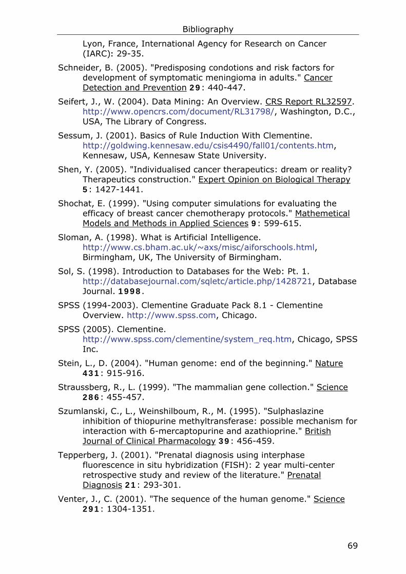
Bibliography

69

Lyon, France, International Agency for Research on Cancer (IARC): 29-35.

Schneider, B. (2005). "Predisposing condotions and risk factors for development of symptomatic meningioma in adults." Cancer Detection and Prevention 29: 440-447.

Seifert, J., W. (2004). Data Mining: An Overview. CRS Report RL32597. http://www.opencrs.com/document/RL31798/, Washington, D.C., USA, The Library of Congress.

Sessum, J. (2001). Basics of Rule Induction With Clementine. http://goldwing.kennesaw.edu/csis4490/fall01/contents.htm, Kennesaw, USA, Kennesaw State University.

Shen, Y. (2005). "Individualised cancer therapeutics: dream or reality? Therapeutics construction." Expert Opinion on Biological Therapy 5: 1427-1441.

Shochat, E. (1999). "Using computer simulations for evaluating the efficacy of breast cancer chemotherapy protocols." Mathemetical Models and Methods in Applied Sciences 9: 599-615.

Sloman, A. (1998). What is Artificial Intelligence. http://www.cs.bham.ac.uk/~axs/misc/aiforschools.html, Birmingham, UK, The University of Birmingham.

Sol, S. (1998). Introduction to Databases for the Web: Pt. 1. http://databasejournal.com/sqletc/article.php/1428721, Database Journal. 1998.

SPSS (1994-2003). Clementine Graduate Pack 8.1 - Clementine Overview. http://www.spss.com, Chicago.

SPSS (2005). Clementine. http://www.spss.com/clementine/system_req.htm, Chicago, SPSS Inc.

Stein, L., D. (2004). "Human genome: end of the beginning." Nature 431: 915-916.

Straussberg, R., L. (1999). "The mammalian gene collection." Science 286: 455-457.

Szumlanski, C., L., Weinshilboum, R., M. (1995). "Sulphaslazine inhibition of thiopurine methyltransferase: possible mechanism for interaction with 6-mercaptopurine and azathioprine." British Journal of Clinical Pharmacology 39: 456-459.

Tepperberg, J. (2001). "Prenatal diagnosis using interphase fluorescence in situ hybridization (FISH): 2 year multi-center retrospective study and review of the literature." Prenatal Diagnosis 21: 293-301.

Venter, J., C. (2001). "The sequence of the human genome." Science 291: 1304-1351.

Bibliography

70

Wang, M. (2004). Storage Device Performance Prediction with CART Models. Joint International Conference on Measurement and Modelling of Computer Systems, New York, New York, ACM Sigmetrics.

Wegener, S. (1998). Zellisolierung. DGI Technisches Handbuch Histokompatibilität und Immungenetik, Methodenkommision der Deutschen Gesellschaft für Immungenetik: 12-41.

Windstosser, K. (1994). "Chemotherapie aus ganzheitlicher Sicht." ECIM-Broschüre 72: 1-15.

Wolberg, W., H. (1990). "Multisurface method of pattern seperation for medical diagnosis applied to breast cytology." Proceedings of the National Acadamy of Sciences, USA 87: 9193-9196.

www.oralcancerfoundation.org (2004). Theranostics: Guiding therapy, Oral cancer foundation.

Xu, C., W. (2002). "High-Density cell microarrays for Parallel functional determinations." Genome Research 12: 482-486.

Yei, C., J. (2005). "Lewis blood genotypes of peptic ulcer and gastric cancer patients in Taiwan." World Journal Gastroenterology 11: 4891-4894.

Ziauddin, J., Sabatini, D., M. (2001). "Microarrays of cells expressing defined cDNAs." Nature 411: 107-110.

Appendix

71

7 Appendix

7.1 IETDB Documentation (IET_Database.info)

The documentation file of the IETDB is accessible via the IET web

interface and is also published on the IET-CD attached to this thesis. It

summarises general information and attribute descriptions for the IET

database and is reprinted below.

Citation Request:

This Immuno Efficiency Test (IET) database was obtained from Davids Biotechnolgie and Dr. Hans-Albert Schöttler. If you publish results when using this database, then please include this information in your acknowledgements.

1. Title: Immuno Efficiency Test (IET) Database (November, 2005)

2. Sources:

-- Dr. Michael Davids (Laboratory)

Davids Biotechnologie

Regensburg,

Germany

-- Donor: Dipl.-Ing. Hans-Albert Schöttler (Physician)

Received by Dipl.-Ing. Hans-Albert Schöttler

-- Date: 01 August 2005

3. Past Usage:

The dataset was used to determine patterns and build predictive models to estimate drug effects.

1. Wolf, A.F-J. (2005). Storage and Analysis of Data Obtained from the Immune Efficiency Test (IET).

4. Relevant Information:

Samples arrive periodically as Dr. Davids and Dipl.-Ing. Schöttler report their clinical cases. The database therefore reflects this chronological grouping of the data. This grouping information appears immediately below.

Appendix

72

Group 1: 1 patient (0.95%) (1999) Group 2: 4 patients (3.81%) (2000) Group 3: 8 patients (7.62%) (2001) Group 4: 24 patients (22.86%) (2002) Group 5: 12 patients (11.43%) (2003) Group 6: 34 patients (32.38%) (2004) Group 7: 22 patients (20.95%) (2005)

-------------------------------------------------

Total: 1241 patients

5. Number of Instances: 1241 (as of 01 August 2005)

6. Number of Attributes: 11

7. Attribute Information:

Attribute Storage Type Data Type Value

Age Real Range [22.5, 91.4]

Blastodermic layer Integer Set 0, 2, 4, 6, 8 Blood Group Integer Set 0, 2, 4, 6, 8 BMI Real Range [16.7, 36.7] Diagnosis ID Integer Set 1,…,24 Drug Group Integer Set 0, 1, 2, 3, 4, 5 Drug ID Integer Set 0,…,56 Lymphocyte No. Real Range [0.31, 4.5] Sex Integer Flag 2, 4 Status Integer Set 0, 2, 4

8. Diagnosis ID: ID Diagnosis ID Diagnosis

1 not known 13 Ovarian Ca. 2 Bronchial Ca. 14 Pancreas Ca. 3 Colon Ca. 15 Prostata Ca. 4 Control 16 Rectum Ca. 5 Esophagus Ca. 17 Renal Ca. 6 Glioma 18 Sigma Ca. 7 Intestinal Ca. 19 Squanous Epithelium Ca. 8 Leukemia 20 Stomach Cancer 9 Malignant Melanoma 21 Uterus Ca. 10 Mamma Ca. 22 Vaginal Ca. 11 Myosarcoma 23 Vesica Ca. 12 Nasopharynx Ca. 24 Immune Deficiency

9. Tumarmarker: CCR, LSA, CEA

CCR [Extension]: Continuous Complete Remission (normal

range<0,8) LSA [mg/100ml]: Lipid bound Sialic Acid (normal

range<22mg/100ml) CEA [ng/ml]: Carcino Embryonic Antigen (normal range

0-3ng/ml)

Appendix

73

10. Class distribution: Benign: 18 (17.14%) Malignant: 81 (77.14%) Not Known: 6 (5.71%)

11. Drug Attribute: Aggregation

Some drugs can be merged based on their chemical structure or groups. All currently known subgroups occurring within the database are listed below:

7.2 Visual Programming in Clementine

Most data mining procedures were performed in Clementine by visual

programming. All implementations in Clementine (called streams) are

summarised in this section.

Data understanding – The stream implementation for data

understanding is shown in Figure 23. First, data type settings for all

attributes were made. This was done using a Type node. Storage types

of the attributes were defined in the InitialDataset node.

Group Drug ID Description

Group 0 0 Control Group 1 37, 41, 50, 56 Enzyme Group 2 13, 18, 22, 25, 26 Mistletoe Group 3 32, 33, 47, 48, 49 Thymus Group 4 30, 54, 55 Vitamin Group 5 All others Others

Appendix

74

7

8

6

5

3

4

2 1

Figure 23 Clementine stream for data understanding. Visualisation of the initial dataset (1) aided to define data mining objectives. Clementine provides a set of tools to promote basic understanding of the dataset. To promote data understanding tables (8), distribution graphs (4), basic statistics tools (6) and general data audit illustrations (5) were used. The Type node (2) is used to define data types of the various attributes. A web graph (7) is used to determine interactions of the Blood Group, Rhesus and Status attributes. A Derive node (3) is used to generate the attribute YearOfTest.

For visualisation of the initial dataset, the Clementine tools Table,

Distribution graph, Statistics and Data Audit were used. In order to

create the new attribute YearOfTest a Derive node was used. Results of

these operations, in particular the distribution of the attributes Sex,

Status and YearOfTest, increase data understanding and are

summarised in the documentation file, IET_Documentation.info. To

identify interactions between the Status, Blood Group and Rhesus

attributes, a Web Graph node was used.

Data Pre-processing – All dataset, data, attribute and formatting

operations performed in Clementine and necessary to create individual

immune efficiency profiles are displayed in Figure 24.

Appendix

75

1 2 3

4

5

6

7

8

13

12

11

10 9

Figure 24 Clementine Stream for Data Pre-processing. The stream shows all operations required to prepare the dataset for modelling.

Before starting data pre-processing in Clementine, the dataset was

transformed from a patient-wise into a drug-wise format by using the

java application Transformer.java. Further, data types and missing

values of the initial dataset (1) are set using a Type node (2). Irrelevant

attributes (Patient_ID, Test_ID and Postcode) were excluded using a

Filter node (3). Data quality analysis was performed using a Quality

node (4) which automatically generates a Filter node (5) to exclude

attributes of insufficient data quality. The derived Age, BMI and Effect

attributes were included by using Derive nodes (6, 7, 8). A Type node

(9) was used to set data types for these attributes. Thus, the original

Date of Birth, Date of Test, Height, Weight and Result attributes were

excluded using a Filter node (10). Data quality was analysed (11) once

more, before accepting all data pre-processing operations by creating a

new data file (12). Finally, the source code of the entire stream was

published using a Publisher node (13). The source code of the stream

can be found on the IET-CD.

Modelling – Before model building was started, the pre-processed

dataset was split into a training and validation set. This was done using

Appendix

76

the java application Randomiser.java. The Clementine stream of the

modelling phase is illustrated in Figure 25.

1

2

7

6

4 5

3

Figure 25 Clementine Stream Implementation for Modelling. In the Modelling phase, the two Clementine algorithms C&Rtree (4) and Neural Network (5) were used for model building.

In the modelling phase the machine learning algorithms C&RTree (4)

and Neural Network (5) used the training set (1) for model building.

Since dataset splitting was performed externally (Sampling methods

provided by Clementine were not sufficient for our purposes; see

Randomiser.java), data types and missing values needed to be defined

again. This was done using a Type node (2). A Quality node (4) was

used to analyse data quality before model building was started.

Evaluation – The evaluation phase (Figure 26) tested how well the two

models (4, 5) performed on the validation set (1). This was done using

Quality nodes (6, 7). The steps (2) and (3) were identical to the

modelling phase. Finally, the stream source code was published for both

models (8, 9). This includes all settings for model building as well.

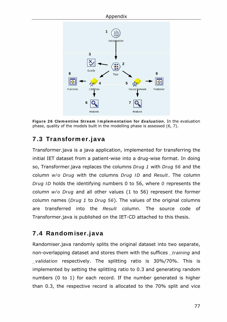
Appendix

77

1

5 4

8 9

6 7

3

2

Figure 26 Clementine Stream Implementation for Evaluation. In the evaluation phase, quality of the models built in the modelling phase is assessed (6, 7).

7.3 Transformer.java

Transformer.java is a java application, implemented for transferring the

initial IET dataset from a patient-wise into a drug-wise format. In doing

so, Transformer.java replaces the columns Drug 1 with Drug 56 and the

column w/o Drug with the columns Drug ID and Result. The column

Drug ID holds the identifying numbers 0 to 56, where 0 represents the

column w/o Drug and all other values (1 to 56) represent the former

column names (Drug 1 to Drug 56). The values of the original columns

are transferred into the Result column. The source code of

Transformer.java is published on the IET-CD attached to this thesis.

7.4 Randomiser.java

Randomiser.java randomly splits the original dataset into two separate,

non-overlapping dataset and stores them with the suffices _training and

_validation respectively. The splitting ratio is 30%/70%. This is

implemented by setting the splitting ratio to 0.3 and generating random

numbers (0 to 1) for each record. If the number generated is higher

than 0.3, the respective record is allocated to the 70% split and vice

Appendix

78

versa. The 30% split is used for validation, the 70% for training. The

source code of Randomiser.java is published on the IET-CD.

7.5 RandomisationTester.java

As input file, RandomisationTester.java takes for example the IET

validation set. The number of permutation and number of bars

parameters for the resulting histogram can be altered in the source

code. By default 10,000 permutations and 50 bars are used.

RandomisationTester.java was implemented to perform randomisation

testing not being provided in Clementine. Here, the class attribute Effect

is randomly shuffled 10,000 times for the given dataset. These

permutations are stored and compared to the original set. This results

in a histogram representing the number of correct predictions by

randomisation testing. The user gets a file with the suffix _histogram

appended to the original file name, including histogram data, along with

the standard deviation and the arithmetic mean. The source code is

published on the IET-CD.

7.6 IET CD

The CD attached to this thesis is meant for specialists interested in the

source code. Here, the source code of the following applications and

implementations is published:

• IET Database – SQL statements for creating the database

• IET Web Interface – All html and php scripts developed for the interface

• Clementine Visual Programming – Code for all relevant streams including those for data pre-processing, modelling and evaluation

• Transformer.java – Source code written in java

• Randomiser.java – Source code written in java

• RandomisationTester.java – Source code written in java

Glossary

79

8 Glossary

CGI

CGI is a standardised web technology for the communication of a client browser and a web server.

CRISP-DM

CRISP-DM is a industry proven standard methodology for data mining.

Data Type

A data type is a named category of data that is characterised by a set of values along with a description to denote those values and a collection of operations that interpret and manipulate the values.

Entity

An entity is something that has a distinct and separate existence. This does not necessarily imply a material existence.

Entity Type

A collection of entities characterised by common properties.

Java

Java is a object-oriented programming language.

JavaScript

JavaScript is a object-based scripting language used to include dynamic elements into web pages.

Kohonen

The kohonen algorithm implements the concept of self organising maps and assigns to unsupervised learning.

PERL

Perl is an interpreted procedural programming language developed by Larry Wall in 1987. Perl is synthesis of C, unix commands and other influences.

Glossary

80

PHP

PHP is a programming language used to create websites. The syntax of php is loosely based on C and Perl.

Primary key

A primary key is a unique identifier (attribute) within a table, that is capable of distinguishing each row from all the other rows.

SQL

SQL is the most commonly used computer language to create, modify and retrieve data from a relational database management system.

Stream programming

Stream programming or visual programming provides an opportunity for the developer to build a program just by plugging pre-written pieces of logic together.

Table

A table is a set of elements with a horizontal dimension (rows) and a vertical dimension (columns).

List of Abbreviations

81

9 List of Abbreviations

ACL Actual Class Label

AI Artificial Intelligence

ANN Artificial Neural Network

CART Classification And Regression Tree

C&Rtree Classification & Regression tree

CGI Common Gateway Interface

CRISP-DM CRoss Industry Standard Process for Data Mining

DBMS DataBase Management System

DMEM Dulbecco/Vogt Modified Eagle’s Minimum Essential Medium

FCS Fetal Calf Serum

FISH Fluorescent In Situ Hybridisation

IET Immune Efficiency Test

ILA Induced Lymphocyte Activity

KDD Knowledge Discovery in Databases

LA Lymphocyte Activity

NchIP Native Chromatin Immuno Precipitation

PCL Predicted Class Label

PCR Polymerase Chain Reaction

PERL Practical Extraction and Report Language

PHP PHP: Hypertext Preprocessor

PK Primary Key

FK Foreign Key

q-PCR q - Polymerase Chain Reaction

RCL Randomised Class Label

List of Abbreviations

82

rt-PCR real time - Polymerase Chain Reaction

SQL Structured Query Language

List of Figures

83

10 List of Figures

Figure 1 Cancer Mortality by Tissue - Leading Causes of Cancer Deaths............................................................................................. 3

Figure 2 Schematic Illustration of the Immune Efficiency Test (IET). ..11 Figure 3 Interpretation of IET Results.............................................15 Figure 4 Turning Limitations into Innovations. .................................16 Figure 5 Three-Tier Client Server Architecture. ................................20 Figure 6 Architecture of Biological and Artificial Neural Networks........24 Figure 7 Decision Tree Built by Applying a CART Algorithm................26 Figure 8 Phases of the CRISP-DM Reference Model. .........................29 Figure 9 Randomisation Testing.....................................................33 Figure 10 Structure and Attributes of a Patient Chart – The Basis for the

Initial Dataset. ......................................................................36 Figure 11 Entity Relationship (E/R) Model .......................................39 Figure 12 Un-normalised Form (UNF) of the IET database. ................40 Figure 13 Normalisation Process....................................................41 Figure 14 Relational Model of the IET-Database in 2NF. ....................42 Figure 15 Data Retrieval. .............................................................44 Figure 16 Data Insertion. .............................................................44 Figure 17 Data Insertion – New Result. ..........................................45 Figure 18 Edit Data. ....................................................................46 Figure 19 Web Graphs of the Attributes Blood Group, Rhesus and

Status..................................................................................51 Figure 20 Dataset Transformation from Patient-wise to Drug-wise

Format.................................................................................53 Figure 21 Compilation of String and Numeric Values of the Respective

Attributes. ............................................................................57 Figure 22 Randomisation Test. ......................................................60 Figure 23 Clementine stream for data understanding. ......................74 Figure 24 Clementine Stream for Data Pre-processing. .....................75 Figure 25 Clementine Stream Implementation for Modelling. .............76 Figure 26 Clementine Stream Implementation for Evaluation.............77

List of Tables

84

11 List of Tables

Table 1 Recent Approaches in Immunotherapy (Jatzko 2005). ............ 5 Table 2 Analogy between Biological and Artificial Neural Networks..... 23 Table 3 Data and Storage Type Settings for the Initial Dataset.......... 37 Table 4 Advices and Consideration Acquired from Data Exploration.... 52 Table 5 Grouping of Drug ID According to Chemical or Structural

properties. ........................................................................... 54 Table 6 Data Quality Report. ........................................................ 55 Table 7 Relationship of the Proliferation Rate and the New Class

Attribute Effect. .................................................................... 56 Table 8 Final Attribute Properties. ................................................. 58 Table 9 Data Mining IET Data....................................................... 61

contentsguanine.evolbio.mpg.de/homepage/wolf.pdf · introduction 3 1 introduction in most western...

Documents