a constrained large time increment method for modelling...
TRANSCRIPT

A constrained LArge Time INcrement method
for modelling quasi-brittle failure
Bram VANDORENa
K. De Profta A. Simoneb L. J. Sluysb
a Hasselt University, Belgium
b Delft University of Technology, The Netherlands
CFRAC 2013, 6th June, 2013, Prague, Czech Republic

Outline
introduction to LArge Time INcrement (LATIN) method
tracing snap-back behaviour within the LATIN method
numerical examples
A constrained LArge Time INcrement method for modelling quasi-brittle failure 1 / 20

LATIN method
non-incremental solution method for non-linear mechanics
[Boisse et al., IJNME 1990; Ladevèze, 1999]
an alternative to step-by-step solution methods
e.g. incremental-iterative Newton-Raphson method
limited range of convergence
requires continuation techniques in case of limit andsnap-back points, i.e. the addition of a constraint equation
to the FE equations [Riks, IJSS 1979; Crisfield, C&S 1981]
continuation techniques: which constraint function?
convergence problems in case of bifurcations
A constrained LArge Time INcrement method for modelling quasi-brittle failure 2 / 20

LATIN method
whole time domain is calculated in one iteration
converged solution is the exact solution
snap-back behaviour cannot be traced
F
u
F
u
t
t+1
A constrained LArge Time INcrement method for modelling quasi-brittle failure 3 / 20
Newton-Raphson LATIN

LATIN method
typically applied to hardening (visco-)plastic and brittle
materials [Abdali et al., JMPT 1996; Dolbow et al., CMAME 2001]
goals of this contribution
application to quasi-brittle materials
tracing snap-back points within LATIN method
A constrained LArge Time INcrement method for modelling quasi-brittle failure 4 / 20

LATIN method: Ingredients
two main solution stages, executed alternately
local solution stage (n + 1/2): local and non-linear
global solution stage (n + 1): global and linear
‘separating the difficulties’ [Ladevèze, 1999]
A constrained LArge Time INcrement method for modelling quasi-brittle failure 5 / 20
(
σn+1/2, εn+1/2
)
(σn, εn)
(σn+1, εn+1)
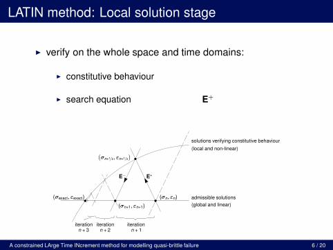
(σexact, εexact) admissible solutions
(global and linear)
solutions verifying constitutive behaviour
(local and non-linear)
E+E−
iterationiterationiterationn + 1n + 2n + 3

LATIN method: Local solution stage
verify on the whole space and time domains:
constitutive behaviour: σn+1/2 = Cεn+1/2
search equation:(
σn+1/2 − σn
)
+ E+(
εn+1/2 − εn
)
= 0
A constrained LArge Time INcrement method for modelling quasi-brittle failure 6 / 20
(
σn+1/2, εn+1/2
)
(σn, εn)
(σn+1, εn+1)
(σexact, εexact) admissible solutions
(global and linear)
solutions verifying constitutive behaviour
(local and non-linear)
E+E−
iterationiterationiterationn + 1n + 2n + 3
LATIN method: Local solution stage
verify on the whole space and time domains:
constitutive behaviour : σn+1/2 = Cεn+1/2
search equation :(
σn+1/2 − σn
)
+E+(
εn+1/2 − εn
)
= 0
A constrained LArge Time INcrement method for modelling quasi-brittle failure 6 / 20
(
σn+1/2, εn+1/2
)
(σn, εn)
(σn+1, εn+1)
(σexact, εexact) admissible solutions
(global and linear)
solutions verifying constitutive behaviour
(local and non-linear)
E+E−
iterationiterationiterationn + 1n + 2n + 3

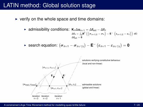
LATIN method: Global solution stage
verify on the whole space and time domains:
admissibility conditions:
search equation:(
σn+1 − σn+1/2
)
− E−
(
εn+1 − εn+1/2
)
= 0
A constrained LArge Time INcrement method for modelling quasi-brittle failure 7 / 20
∫
Ωδε(σn+1 − σn) dΩ =∫
Γtδu
(
tn+1 − tn
)
dΓt
with σ S. A. and u K. A.
(
σn+1/2, εn+1/2
)
(σn, εn)
(σn+1, εn+1)
(σexact, εexact) admissible solutions
(global and linear)
solutions verifying constitutive behaviour
(local and non-linear)
E+E−
iterationiterationiterationn + 1n + 2n + 3
LATIN method: Global solution stage
verify on the whole space and time domains:
admissibility conditions:
search equation:(
σn+1 − σn+1/2
)
− E−
(
εn+1 − εn+1/2
)
= 0
A constrained LArge Time INcrement method for modelling quasi-brittle failure 7 / 20
Kn∆un+1 = ∆fext −∆fn
∆fn =∫
ΩBT((
σn+1/2 − σn
)
− E−
(
εn+1/2 − εn
))
dΩ
∆fext = 0
(
σn+1/2, εn+1/2
)
(σn, εn)
(σn+1, εn+1)
(σexact, εexact) admissible solutions
(global and linear)
solutions verifying constitutive behaviour
(local and non-linear)
E+E−
iterationiterationiterationn + 1n + 2n + 3

LATIN method: Global solution stage
verify on the whole space and time domains:
admissibility conditions:
search equation :(
σn+1 − σn+1/2
)
−E−
(
εn+1 − εn+1/2
)
= 0
A constrained LArge Time INcrement method for modelling quasi-brittle failure 7 / 20
Kn∆un+1 = ∆fext −∆fn
∆fn =∫
ΩBT((
σn+1/2 − σn
)
− E−
(
εn+1/2 − εn
))
dΩ
∆fext = 0
(
σn+1/2, εn+1/2
)
(σn, εn)
(σn+1, εn+1)
(σexact, εexact) admissible solutions
(global and linear)
solutions verifying constitutive behaviour
(local and non-linear)
E+E−
iterationiterationiterationn + 1n + 2n + 3
LATIN method: Tracing snap-back behaviour
one option: switch to classical Newton-Raphson algorithmnear the snap-back point [Kerfriden et al., CM 2009]
complicates the algorithm
which constraint function?
an alternative: add a constraint function to the globalsolution stage of the LATIN algorithm
‘stand-alone’ LATIN algorithm
which constraint function?
A constrained LArge Time INcrement method for modelling quasi-brittle failure 8 / 20

LATIN method: Tracing snap-back behaviour
classical constrained Newton-Raphson method
constraint function defined in terms of incremental
displacement field
constrained LATIN method
no previous converged load step
constraint function in terms of thetotal displacement field, e.g.
un+1TAun+1 − τ2 = 0
A selects a subset of DOF’s[Geers, IJNME 1999]
A constrained LArge Time INcrement method for modelling quasi-brittle failure 9 / 20
τ
u2u1
λ
u
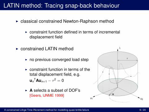
LATIN method: Tracing snap-back behaviour
classical constrained Newton-Raphson method
constraint function defined in terms of incremental
displacement field
constrained LATIN method
no previous converged load step
constraint function in terms of thetotal displacement field, e.g.
unTAun+1 − τ2 = 0
A selects a subset of DOF’s[Geers, IJNME 1999]
A constrained LArge Time INcrement method for modelling quasi-brittle failure 9 / 20
τ
u2u1
λ
u

LATIN method: Global solution stage
verify on the whole space and time domains:
admissibility conditions:
search equation:(
σn+1 − σn+1/2
)
− E−
(
εn+1 − εn+1/2
)
= 0
A constrained LArge Time INcrement method for modelling quasi-brittle failure 10 / 20
Kn∆un+1 = ∆fext −∆fn
∆fn =∫
ΩBT((
σn+1/2 − σn
)
− E−
(
εn+1/2 − εn
))
dΩ
∆fext = 0∆λn+1 fext
(
σn+1/2, εn+1/2
)
(σn, εn)
(σn+1, εn+1)
(σexact, εexact) admissible solutions
(global and linear)
solutions verifying constitutive behaviour
(local and non-linear)
E+E−
iterationiterationiterationn + 1n + 2n + 3

Constrained LATIN method: Global solution stage
verify on the whole space and time domains:
admissibility conditions:
search equation:(
σn+1 − σn+1/2
)
− E−
(
εn+1 − εn+1/2
)
= 0
constraint equation: unTAun+1 − τ2 = 0
A constrained LArge Time INcrement method for modelling quasi-brittle failure 10 / 20
Kn∆un+1 = ∆fext −∆fn
∆fn =∫
ΩBT((
σn+1/2 − σn
)
− E−
(
εn+1/2 − εn
))
dΩ
∆fext = ∆λn+1 fext
(
σn+1/2, εn+1/2
)
(σn, εn)
(σn+1, εn+1)
(σexact, εexact) admissible solutions
(global and linear)
solutions verifying constitutive behaviour
(local and non-linear)
E+E−
iterationiterationiterationn + 1n + 2n + 3

Constrained LATIN method: Global solution stage
verify on the whole space and time domains:
admissibility conditions :
search equation :(
σn+1 − σn+1/2
)
−E−
(
εn+1 − εn+1/2
)
= 0
constraint equation: unTAun+1 − τ2 = 0
A constrained LArge Time INcrement method for modelling quasi-brittle failure 10 / 20
Kn∆un+1 = ∆fext −∆fn
∆fn =∫
ΩBT((
σn+1/2 − σn
)
− E−
(
εn+1/2 − εn
))
dΩ
∆fext = ∆λn+1 fext
(
σn+1/2, εn+1/2
)
(σn, εn)
(σn+1, εn+1)
(σexact, εexact) admissible solutions
(global and linear)
solutions verifying constitutive behaviour
(local and non-linear)
E+E−
iterationiterationiterationn + 1n + 2n + 3

Numerical examples
masonry wall under shear loading
fracture of a perforated cantilever beam
A constrained LArge Time INcrement method for modelling quasi-brittle failure 11 / 20

Numerical examples: Masonry wall
linear elastic bricks and exponential damage law in mortarjoints (modelled as interface-like elements [Simone, CNME 2004])
tint = (1 − ω)dint[[u]]int
degenerated capped Drucker-Prager material model
[Vandoren et al., CMAME 2013]
A constrained LArge Time INcrement method for modelling quasi-brittle failure 12 / 20
0.30 N/mm2
990
70
70
1106
F bricks: 52 mm × 210 mm× 100 mm
hjoints = 10 mm
Ebrick = 16700 N/mm2
νbrick = 0.15
dn,int = 82 N/mm3
dt,int = 36 N/mm3
ft,int = 0.25 N/mm2
fc,int = 10.5 N/mm2
GfI,int = 0.018 N/mm
[Raijmakers and Vermeltfoort, 1992]
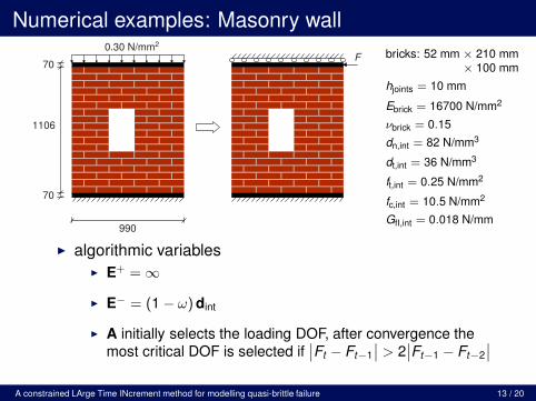
Numerical examples: Masonry wall
algorithmic variables
E+ = ∞
E− = (1 − ω)dint
A initially selects the loading DOF, after convergence the
most critical DOF is selected if∣
∣Ft − Ft−1
∣
∣ > 2∣
∣Ft−1 − Ft−2
∣
∣
A constrained LArge Time INcrement method for modelling quasi-brittle failure 13 / 20
0.30 N/mm2
990
70
70
1106
F bricks: 52 mm × 210 mm× 100 mm
hjoints = 10 mm
Ebrick = 16700 N/mm2
νbrick = 0.15
dn,int = 82 N/mm3
dt,int = 36 N/mm3
ft,int = 0.25 N/mm2
fc,int = 10.5 N/mm2
GfI,int = 0.018 N/mm

Numerical examples: Masonry wall
0 1 2 3 4 50
10
20
30
40
50iteration 1
displacement [mm]
forc
e [k
N]
A constrained LArge Time INcrement method for modelling quasi-brittle failure 14 / 20

Numerical examples: Masonry wall
A constrained LArge Time INcrement method for modelling quasi-brittle failure 14 / 20

Numerical examples: Masonry wall
0 1 2 3 4 50
10
20
30
40
50
displacement [mm]
forc
e [k
N]
A constrained LArge Time INcrement method for modelling quasi-brittle failure 15 / 20

Numerical examples: Masonry wall
A constrained LArge Time INcrement method for modelling quasi-brittle failure 15 / 20

Numerical examples: Perforated beam
non-linear interface element along horizontal axis of
symmetry: linear cohesive damage law
tint = (1 − ω)dint[[u]]int
damage driven by [[un]]int
A constrained LArge Time INcrement method for modelling quasi-brittle failure 16 / 20
0.2 0.375
1.5
1.0
F
F
Ebeam = 100 N/mm2
νbeam = 0.30
dn,int = 10000 N/mm3
dt,int = 5000 N/mm3
ft,int = 1.0 N/mm2
GfI,int = 2.5 · 10−3 N/mm
[Verhoosel et al., IJNME 2009]

Numerical examples: Perforated beam
algorithmic variables
E+ = ∞
E− = (1 − ω)dint
A initially selects the loading DOF, after convergence the
most critical DOF is selected if∣
∣Ft − Ft−1
∣
∣ > 2∣
∣Ft−1 − Ft−2
∣
∣
A constrained LArge Time INcrement method for modelling quasi-brittle failure 17 / 20
0.2 0.375
1.5
1.0
F
F
Ebeam = 100 N/mm2
νbeam = 0.30
dn,int = 10000 N/mm3
dt,int = 5000 N/mm3
ft,int = 1.0 N/mm2
GfI,int = 2.5 · 10−3 N/mm

Numerical examples: Perforated beam
0 0.01 0.02 0.030
0.02
0.04
0.06
0.08
0.1
0.12iteration 1
displacement [mm]
forc
e [N
]
A constrained LArge Time INcrement method for modelling quasi-brittle failure 18 / 20

Numerical examples: Perforated beam
A constrained LArge Time INcrement method for modelling quasi-brittle failure 18 / 20

Numerical examples: Perforated beam
0 0.01 0.02 0.03
0.02
0.04
0.06
0.08
0.1
displacement [mm]
forc
e [N
]
A constrained LArge Time INcrement method for modelling quasi-brittle failure 19 / 20

Numerical examples: Perforated beam
A constrained LArge Time INcrement method for modelling quasi-brittle failure 19 / 20

Conclusions
constrained LATIN method
now possible to trace snap-backs within LATIN method
most critical DOF’s in the constraint function are
automatically detected
linear convergence rate (with the current search directions)
a robust alternative to conventional step-by-step methods
future work
optimise search directions
A constrained LArge Time INcrement method for modelling quasi-brittle failure 20 / 20