a convex variational model for restoring blurred images with multiplicative noise

General rights Copyright and moral rights for the publications made accessible in the public portal are retained by the authors and/or other copyright owners and it is a condition of accessing publications that users recognise and abide by the legal requirements associated with these rights.

Users may download and print one copy of any publication from the public portal for the purpose of private study or research.

You may not further distribute the material or use it for any profit-making activity or commercial gain

You may freely distribute the URL identifying the publication in the public portal If you believe that this document breaches copyright please contact us providing details, and we will remove access to the work immediately and investigate your claim.

Downloaded from orbit.dtu.dk on: Jan 06, 2019

A Convex Variational Model for Restoring Blurred Images with Multiplicative Noise

Dong, Yiqiu; Tieyong Zeng

Published in:S I A M Journal on Imaging Sciences

Link to article, DOI:10.1137/120870621

Publication date:2013

Document VersionPublisher's PDF, also known as Version of record

Link back to DTU Orbit

Citation (APA):Dong, Y., & Tieyong Zeng (2013). A Convex Variational Model for Restoring Blurred Images with MultiplicativeNoise. S I A M Journal on Imaging Sciences, 6(3), 1598-1625. DOI: 10.1137/120870621

https://doi.org/10.1137/120870621

http://orbit.dtu.dk/en/publications/a-convex-variational-model-for-restoring-blurred-images-with-multiplicative-noise(de96c2c7-bb64-4f68-a29e-6c5fc2461447).html

Copyright © by SIAM. Unauthorized reproduction of this article is prohibited.

SIAM J. IMAGING SCIENCES c© 2013 Society for Industrial and Applied MathematicsVol. 6, No. 3, pp. 1598–1625

A Convex Variational Model for Restoring Blurred Images with MultiplicativeNoise∗

Yiqiu Dong† and Tieyong Zeng‡

Abstract. In this paper, a new variational model for restoring blurred images with multiplicative noise isproposed. Based on the statistical property of the noise, a quadratic penalty function techniqueis utilized in order to obtain a strictly convex model under a mild condition, which guaranteesthe uniqueness of the solution and the stabilization of the algorithm. For solving the new convexvariational model, a primal-dual algorithm is proposed, and its convergence is studied. The paperends with a report on numerical tests for the simultaneous deblurring and denoising of images subjectto multiplicative noise. A comparison with other methods is provided as well.

Key words. convexity, deblurring, multiplicative noise, primal-dual algorithm, total variation regularization,variational model

AMS subject classifications. 52A41, 65K10, 65K15, 90C30, 90C47

DOI. 10.1137/120870621

1. Introduction. In real applications, degradation effects are unavoidable during imageacquisition and transmission. For instance, the photos produced by astronomical telescopesare often blurred by atmospheric turbulence. In order to further improve image processingtasks, image deblurring and denoising continue to attract attention in the applied mathematicscommunity. Based on the imaging systems, various kinds of noise were considered, such asadditive Gaussian noise, impulse noise, and Poisson noise. We refer the reader to [17, 21, 35,40, 44, 45] and references therein for an overview of those noise models and the restorationmethods. However, multiplicative noise is a different noise model, and it commonly appears insynthetic aperture radar (SAR), ultrasound imaging, laser images, and so on [8, 9, 39, 43]. Fora mathematical description of such degradations, suppose that an image u is a real functiondefined on Ω, a connected bounded open subset of R2 with compact Lipschitz boundary, i.e.,u : Ω → R. The degraded image f is given by

(1.1) f = (Au)η,

where A ∈ L(L2(Ω)) is a known linear and continuous blurring operator and η ∈ L2(Ω)represents multiplicative noise with mean 1. Here, f is obtained from u, which is blurredby the blurring operator A, and then is corrupted by the multiplicative noise η. Usuallywe assume that f > 0. In this paper, we concentrate on the assumption that η follows a

∗Received by the editors March 20, 2012; accepted for publication (in revised form) May 29, 2013; publishedelectronically August 22, 2013. This work was supported by RGC 211710, RGC 211911, NSFC 11271049, and theFRGs of Hong Kong Baptist University.

http://www.siam.org/journals/siims/6-3/87062.html†Department of Applied Mathematics and Computer Science, Technical University of Denmark, 2800 Kgs. Lyngby,

Denmark ([email protected]).‡Department of Mathematics, Hong Kong Baptist University, Kowloon Tong, Hong Kong ([email protected]).

1598

Dow

nloa

ded

10/0

3/13

to 1

92.3

8.67

.112

. Red

istr

ibut

ion

subj

ect t

o SI

AM

lice

nse

or c

opyr

ight

; see

http

://w

ww

.sia

m.o

rg/jo

urna

ls/o

jsa.

php

http://www.siam.org/journals/siims/6-3/87062.html

mailto:[email protected]

mailto:[email protected]


CONVEX MULTIPLICATIVE RESTORATION MODEL 1599

Gamma distribution, which commonly occurs in SAR. The deblurring process under noise iswell known to be an ill-posed problem in the sense of Hadamard [30]. Since the degradedimage provides only partial restrictions on the original data, there exist various solutionswhich can match the observed degraded image under the given blurring operator. Hence, inorder to utilize variational methods, the main challenge in image restoration is to design areasonable and easily solved optimization problem based on the degradation model and theprior information on the original image.

Until the past decade, a few variational methods have been proposed to handle the restora-tion problem with the multiplicative noise. Given the statistical properties of the multiplica-tive noise η, in [39] the recovery of the image u was based on solving the following constrainedoptimization problem:

(1.2)

infu∈S(Ω)

∫Ω|Du|

subject to

∫Ω

f

Audx = 1,

∫Ω

(f

Au− 1

)2

dx = θ2,

where θ2 denotes the variance of η, S(Ω) = {v ∈ BV (Ω) : v > 0}, BV (Ω) is the space offunctions of bounded variation (see [6] or below), and the total variation (TV) of u is utilizedas the objective function in order to preserve significant edges in images. In (1.2), onlybasic statistical properties, the mean and the variance, of the noise η are considered, whichsomehow limits the restored results. For this reason, based on the Bayes rule and Gammadistribution with mean 1, by using a maximum a posteriori (MAP) estimator, Aubert andAujol [5] introduced a variational model as follows:

(1.3) infu∈S(Ω)

∫Ω

(log(Au) +

f

Au

)dx+ λ

∫Ω|Du|,

where the TV of u is utilized as the regularization term and λ > 0 is the regularizationparameter which controls the trade-off between a good fit of f and a smoothness requirementdue to the TV regularization. Below we refer to (1.3) as the AA model. Since both (1.2) and(1.3) are nonconvex, the gradient projection algorithms proposed in [39] and [5] may stickat some local minimizers, and the restored results strongly rely on the initialization and thenumerical schemes. To overcome this problem and provide a convex model, in [32] Huang, Ng,and Wen introduced an auxiliary variable z = log u in (1.3), and in [41] Shi and Osher modified(1.3) by adding a quadratic term. With convex models, these two methods both providebetter restored results than the method proposed in [5], and they are independent of the initialestimations. In addition, Steidl and Teubner [42] combined the I-divergence as the data fidelityterm with the TV regularization or the nonlocal means to remove the multiplicative Gammanoise. A general patch-based denoising filter was proposed in [20]. In [22], the denoisingproblem was handled by using a L1 fidelity term on frame coefficients. In [36], the approachwith spatially varying regularization parameters in the AA model (1.3) was considered inorder to restore more texture details of the denoised image. In [31], the multiplicative noiseD

ownl

oade

d 10

/03/

13 to

192

.38.

67.1

12. R

edis

trib

utio

n su

bjec

t to

SIA

M li

cens

e or

cop

yrig

ht; s

ee h

ttp://

ww

w.s

iam

.org

/jour

nals

/ojs

a.ph

p


1600 YIQIU DONG AND TIEYONG ZENG

removal was addressed via a learned dictionary, and extensive experimental results illustratedthe leading performance of this approach. However, all of the above methods work only onthe multiplicative noise removal issue, and it is still an open question to extend them to thedeblurring case.

In this paper, we focus on the restoration of images that are simultaneously blurred andcorrupted by multiplicative noise. Since the nonconvexity of the model (1.3) proposed in [5]causes a uniqueness problem and the issue of convergence of the numerical algorithm, weintroduce a new convex model by adding a quadratic penalty term based on the statisti-cal properties of the multiplicative Gamma noise. Furthermore, we study the existence anduniqueness of a solution to the new model on the continuous, i.e., functional space, level.Here, we still use the TV regularization in order to preserve edges during the reconstruc-tion. Evidently, it can be readily extended to some other modern regularization terms suchas nonlocal TV [26] or the framelet approach [12]. The minimization problem in our methodis solved by the primal-dual algorithm proposed in [15, 24] instead of the gradient projec-tion method in [5, 39]. The numerical results in this paper show that our method has thepotential to outperform the other approaches in multiplicative noise removal with deblurringsimultaneously.

The rest of the paper is organized as follows. In section 2, we briefly review the TVregularization and provide its main properties. In section 3, based on the statistical propertiesof the multiplicative Gamma noise, we propose a new convex model for denoising and studythe existence and uniqueness of a solution with several other properties. Then in section 4 weextend the model and those properties to the case of denoising and deblurring simultaneously.Section 5 gives the primal-dual algorithm for solving our restoration model based on the workproposed in [15]. The numerical results shown in section 6 demonstrate the efficiency of thenew method. Finally, conclusions are drawn in section 7.

2. Review of TV regularization. In order to preserve significant edges in images, intheir seminal work [40] Rudin, Lions, and Osher, introduced TV regularization into imagerestoration. In this approach, they recover the image in BV (Ω), which denotes the space offunctions of bounded variation (BV); i.e., u ∈ BV (Ω) iff u ∈ L1(Ω) and the BV-seminorm,

(2.1)

∫Ω|Du| := sup

{∫Ωu · div(ξ(x))dx∣∣ξ ∈ C∞

0 (Ω,R2), ‖ξ‖L∞(Ω,R2) ≤ 1

},

is finite. The space BV (Ω) endowed with the norm ‖u‖BV = ‖u‖L1 +∫Ω |Du| is a Banach

space. If u ∈ BV (Ω), the distributional derivative Du is a bounded Radon measure, andthe above quantity defined in (2.1) corresponds to the total variation (TV). Based on thecompactness of BV (Ω), in the two-dimensional case we have the embedding BV (Ω) ↪→ Lp(Ω)for 1 ≤ p ≤ 2, which is compact for p < 2. See [3, 6, 16] for more details.

3. A convex multiplicative denoising model. To propose a convex multiplicative denois-ing model, we start from the multiplicative Gamma noise. Suppose that the random variableη follows a Gamma distribution; i.e., its probability density function (PDF) is

(3.1) pη(x; θ,K) =1

θKΓ(K)xK−1e−

xθ for x ≥ 0,

Dow

nloa

ded

10/0

3/13

to 1

92.3

8.67

.112

. Red

istr

ibut

ion

subj

ect t

o SI

AM

lice

nse

or c

opyr

ight

; see

http

://w

ww

.sia

m.o

rg/jo

urna

ls/o

jsa.

php



where Γ is the usual Gamma-function, and θ and K denote the scale and shape parameters,respectively, in the Gamma distribution. Furthermore, the mean of η is Kθ, and the varianceof η is Kθ2; see [29]. As multiplicative noise, in general we assume that the mean of η equals1; then we have that Kθ = 1 and its variance is 1

K .Now, set a random variable Y = 1√

η , whose PDF is

(3.2) pY (y) =2

θKΓ(K)y−2K−1e

− 1θy2 for y ≥ 0.

We can prove the following properties of Y .Proposition 3.1. Suppose that the random variable η follows a Gamma distribution with

mean 1. Set Y = 1√η . Then the means of Y and Y 2 are

E(Y ) =

√KΓ(K − 1/2)

Γ(K)and E(Y 2) =

K

K − 1,

respectively. Furthermore, we have

E(Y n) =K

n2 Γ(K − n

2 )

Γ(K)

for any n ∈ N.Proof. Based on the PDF of η shown in (3.1) and Kθ = 1, we obtain

E(Y ) =

∫ +∞

0

1√x

1

θKΓ(K)xK−1e−

xθ dx

=Γ(K − 1/2)√

θΓ(K)

∫ +∞

0

1

θK−1/2Γ(K − 1/2)xK−3/2e−

xθ dx

=Γ(K − 1/2)√

θΓ(K)

∫ +∞

0pη(x; θ,K − 1/2) dx

=

√KΓ(K − 1/2)

Γ(K).

Similarly, we have

E(Y 2) =

∫ +∞

0

1

x

1

θKΓ(K)xK−1e−

xθ dx

=Γ(K − 1)

θΓ(K)

∫ +∞

0

1

θK−1Γ(K − 1)xK−2e−

xθ dx

=K

K − 1.

Further, for any n ∈ N we can calculate E(Y n) similarly, and obtain

E(Y n) =K

n2 Γ(K − n

2 )

Γ(K).

Dow

nloa

ded

10/0

3/13

to 1

92.3

8.67

.112

. Red

istr

ibut

ion

subj

ect t

o SI

AM

lice

nse

or c

opyr

ight

; see

http

://w

ww

.sia

m.o

rg/jo

urna

ls/o

jsa.

php



Table 1The values of E((Y − 1)2) and the KL divergence of Y with the Gaussian distribution N (μK , σ2

K) fordifferent values of K.

K 4 6 10 20 30

E((Y − 1)2) 0.1178 0.0631 0.0320 0.0141 0.0090

DKL(Y ||N (μK , σ2K)) 0.0114 0.0068 0.0035 0.0014 8.5739e-04

According to the properties of the Gamma function [4] and Proposition 3.1, if K is large,the mean of Y is close to 1. Furthermore, we have the following result.

Proposition 3.2. Suppose that the random variable η follows a Gamma distribution withmean 1. Set Y = 1√

η . Then

(3.3) limK→+∞

E((Y − 1)2) = 0.

Proof. With Proposition 3.1, we readily have

E((Y − 1)2) =K

K − 1− 2

√KΓ(K − 1/2)

Γ(K)+ 1.

Based on the property of the Gamma function (see [4]),

limK→+∞

Γ(K + α)

Γ(K)Kα= 1 ∀α ∈ R;

taking α = −12 , we can immediately obtain

limK→+∞

E((Y − 1)2) = 0.

Proposition 3.2 ensures that the value of E((Y − 1)2) is small with a large K. On theother hand, from Table 1 we can see that, even with a small K, its value is still rather small.

Remark 3.3. Since pY (y) defined in (3.2) is monotonic on either side of the single maximalpoint y = 1 − θ

2 , it is a strictly unimodal function. In statistics, a Gaussian distribution iscommonly used to approximate the unimodal or other distributions; see [23, 38]. To furtherunderstand the relationship between Y and a Gaussian distribution, we need the concept ofthe Kullback–Leibler (KL) divergence. Suppose that P andQ are continuous random variableswith the PDFs p(x) and q(x), respectively. The KL divergence of P and Q is defined as

DKL(P ||Q) :=

∫ ∞

−∞log

(p(x)

q(x)

)p(x) dx,

which is always nonnegative and is zero iff P = Q almost everywhere; see [7]. Based on thePDF of the random variable Y , we can prove that the KL divergence of Y with the Gaussiandistribution N (μK , σ

2K) tends to 0 when K goes to infinity, where μK and σ2K are the mean

and variance of Y , respectively; i.e.,

(3.4) μK := E(Y ) and σK :=√

E(Y 2)− (E(Y ))2.

Proposition 3.4. Suppose that the random variable η follows a Gamma distribution withmean 1. Set Y = 1√

η . Then we have the following:Dow

nloa

ded

10/0

3/13

to 1

92.3

8.67

.112

. Red

istr

ibut

ion

subj

ect t

o SI

AM

lice

nse

or c

opyr

ight

; see

http

://w

ww

.sia

m.o

rg/jo

urna

ls/o

jsa.

php



0 0.5 1 1.5 2 2.5 30

0.2

0.4

0.6

0.8

1

1.2

1.4

1.6

1.8

2

y

p(y)

pY(y)

pN(μ,σ2

)(y)

(a)

0 0.5 1 1.5 2 2.5 30

0.5

1

1.5

2

2.5

y

p(y)

p

Y(y)

pN(μ,σ2

)(y)

(b)

0 0.5 1 1.5 2 2.5 30

0.5

1

1.5

2

2.5

3

3.5

4

4.5

y

p(y)

pY(y)

pN(μ,σ2

)(y)

(c)

Figure 1. Comparisons of the PDFs of Y and N (μK , σ2K) with different K. (a) K = 6, (b) K = 10,

(c) K = 30.

(i)∫ +∞0 pY (y) log pY (y)dy = log 2 − log(

√KΓ(K)) + 2K+1

2 ψ(K) − K, where ψ(K) :=d log Γ(K)

dK is the digamma function (see [2]);

(ii)∫ +∞0 pY (y) log pN (μK ,σ2

K)(y)dy = −12 log(2πeσ

2K), where pN (μK ,σ2

K)(y) denotes the PDF

of the Gaussian distribution N (μK , σ2K);

(iii) limK→+∞DKL(Y ||N (μK , σ2K)) = 0.

Proof. For the proof, see Appendix I (section 8).

Furthermore, let us consider a rescaled version of Y , the random variable Z := Y−μKσK

.When K goes to infinity, Y degenerates to 1; however, Z tends to follow the Gaussian distri-bution N (0, 1). Further, based on Proposition 3.4, we have

limK→+∞

DKL(Z||N (0, 1)) = limK→+∞

DKL(Y ||N (μK , σ2K)) = 0.

Using Proposition 3.4 and the definition of the KL divergence, in Table 1 we list theKL divergence between Y and the Gaussian distribution N (μK , σ

2K) with respect to different

values of K. Obviously, even with small K, DKL(Y ||N (μK , σ2K)) is already very small. In

addition, in Figure 1 we show the PDFs of Y and N (μK , σ2K) with K = 6, K = 10, and

K = 30. We can see that the PDF of Y decreases quickly and is close to symmetry as Kincreases, which are the essential properties of Gaussian distribution.

In the denoising case, that is, where A is the identity operator, from the degradation model

(1.1) we obtain that Y = 1√η =

√uf . Inspired by (3.3), we introduce a quadratic penalty term

into the AA model (1.3), which turns out to be

(3.5) infu∈S(Ω)

E(u) :=

∫Ω

(log u+

f

u

)dx+ α

∫Ω

(√u

f− 1

)2

dx+ λ

∫Ω|Du|

with the penalty parameter α > 0. In addition, we set

S(Ω) := {v ∈ BV (Ω) : v ≥ 0},

which is closed and convex, and we define log 0 = −∞ and 10 = +∞. Note that as f > 0, we

need not define 00 .D

ownl

oade

d 10

/03/

13 to

192

.38.

67.1

12. R

edis

trib

utio

n su

bjec

t to

SIA

M li

cens

e or

cop

yrig

ht; s

ee h

ttp://

ww

w.s

iam

.org

/jour

nals

/ojs

a.ph

p



3.1. Existence and uniqueness of a solution. For the existence and uniqueness of asolution to (3.5), we start with discussing the convexity of the model. Since the quadraticpenalty term provides extra convexity, we prove that E(u) in (3.5) is convex if the parameterα satisfies certain condition.

Proposition 3.5. If α ≥ 2√6

9 , then the model (3.5) is strictly convex.Proof. With t ∈ R

+ and a fixed α, we define a function g as

g(t) := log t+1

t+ α(

√t− 1)2.

Easily, we have that the second order derivative of g satisfies

g′′(t) = −t−2 + 2t−3 +α

2t−

32 .

A direct computation shows that the function t32 g′′(t) reaches its unique minimum, 9α−2

√6

18 ,

at t = 6. Hence, if α ≥ 2√6

9 , we have g′′(t) ≥ 0; i.e., g is convex. Furthermore, since the

function g has only one minimizer, g is strictly convex when α ≥ 2√6

9 .

Setting t = u(x)f(x) for each x ∈ Ω, we obtain the strict convexity of the first two terms

in (3.5). Based on the convexity of the TV regularization, we deduce that E(u) in (3.5) is

strictly convex if α ≥ 2√6

9 . Since the feasible set S(Ω) is convex, the assertion is an immediateconsequence.

Based on Proposition 3.5, we see that, with a suitable α, (3.5) is a convex approximationof the nonconvex model (1.3) with A as the identity operator. Now, we argue the existenceand uniqueness of a solution to (3.5) and the minimum-maximum principle.

Theorem 3.6. Let f be in L∞(Ω) with infΩ f > 0; then the model (3.5) has a solution u∗

in BV (Ω) satisfying0 < inf

Ωf ≤ u∗ ≤ sup

Ωf.

Moreover, if α ≥ 2√6

9 , the solution of (3.5) is unique.Proof. Set c1 := infΩ f , c2 := supΩ f , and let

E0(u) :=

∫Ω

(log u+

f

u

)dx+ α

∫Ω

(√u

f− 1

)2

dx.

For each fixed x ∈ Ω, easily we have log t+ f(x)t ≥ 1 + log f(x) with t ∈ R

+ ∪ {0}. Notingthat E(u) is defined in (3.5), we thus have

E(u) ≥∫Ω

(log u+

f

u

)dx ≥

∫Ω(1 + log f) dx.

In other words, E(u) in (3.5) is bounded from below, and we can choose a minimizingsequence {un ∈ S(Ω) : n = 1, 2, . . .}.

Since for each fixed x ∈ Ω the real function on R+ ∪ {0},

g(t) := log t+f(x)

t+ α

(√t

f(x)− 1

)2

,

Dow

nloa

ded

10/0

3/13

to 1

92.3

8.67

.112

. Red

istr

ibut

ion

subj

ect t

o SI

AM

lice

nse

or c

opyr

ight

; see

http

://w

ww

.sia

m.o

rg/jo

urna

ls/o

jsa.

php



is decreasing if t ∈ [0, f(x)) and increasing if t ∈ (f(x),+∞), one always has g(min(t,M)) ≤g(t) with M ≥ f(x). Hence, we obtain that

E0(inf(u, c2)) ≤ E0(u).

Combining this with∫Ω |D inf(u, c2)| ≤

∫Ω |Du| (see Lemma 1 in section 4.3 of [34]), we have

E(inf(u, c2)) ≤ E(u). In the same way we are able to get E(sup(u, c1)) ≤ E(u). Hence, wecan assume that 0 < c1 ≤ un ≤ c2, which implies that un is bounded in L1(Ω).

As {un} is a minimizing sequence, we know that E(un) is bounded. Furthermore,∫Ω |Dun|

is bounded, and {un} is bounded in BV (Ω). Therefore, there exists a subsequence {unk} which

converges strongly in L1(Ω) to some u∗ ∈ BV (Ω), and {Dunk} converges weakly as a measure

toDu∗ [6]. Since S(Ω) is closed and convex, by the lower semicontinuity of the TV and Fatou’slemma, we get that u∗ is a solution of the model (3.5), and necessarily 0 < c1 ≤ u∗ ≤ c2.

Moreover, if α ≥ 2√6

9 , uniqueness follows directly from the strict convexity of the functionE.

As for Theorem 4.1 in [5], here we also need the assumption infΩ f > 0, which ensures thelower boundedness of E(u) defined in (3.5). In numerical practice, this assumption is alwayskept by using max(f, ε) as the observed image with a very small positive value ε.

In [5] a comparison principle was given concerning the model (1.3). With the α-term in(3.5), it is satisfied with certain conditions on α as well.

Proposition 3.7. Let f1 and f2 be in L∞(Ω) with a1 > 0 and a2 > 0, where a1 = infΩ f1and a2 = infΩ f2. Further, set b1 = supΩ f1 and b2 = supΩ f2. Assume f1 < f2. Suppose u∗1(resp., u∗2) is a solution of (3.5) with f = f1 (resp., f = f2). Then when α < a1a2

b1b2−a1a2, we

have u∗1 ≤ u∗2.Proof. Referring to [5], we define u ∧ v = inf(u, v) and u ∨ v = sup(u, v). Since u∗i is a

minimizer of E(u) with f = fi, which is defined in (3.5), with respect to i = 1, 2, we have

E(u∗1 ∧ u∗2) + E(u∗1 ∨ u∗2) ≥ E(u∗1) + E(u∗2).

Based on the result∫Ω |D(u∗1 ∧ u∗2)|+

∫Ω |D(u∗1 ∨u∗2)| ≤

∫Ω |Du∗1|+

∫Ω |Du∗2| in [13, 27], we get

∫Ω

⎡⎣log(u∗1 ∧ u∗2) + f1

u∗1 ∧ u∗2+ α

(√u∗1 ∧ u∗2f1

− 1

)2⎤⎦ dx

+

∫Ω

⎡⎣log(u∗1 ∨ u∗2) + f2

u∗1 ∨ u∗2+ α

(√u∗1 ∨ u∗2f2

− 1

)2⎤⎦ dx

≥∫Ω

⎡⎣log u∗1 + f1

u∗1+ α

(√u∗1f1

− 1

)2⎤⎦ dx

+

∫Ω

⎡⎣log u∗2 + f2

u∗2+ α

(√u∗2f2

− 1

)2⎤⎦ dx.

Dow

nloa

ded

10/0

3/13

to 1

92.3

8.67

.112

. Red

istr

ibut

ion

subj

ect t

o SI

AM

lice

nse

or c

opyr

ight

; see

http

://w

ww

.sia

m.o

rg/jo

urna

ls/o

jsa.

php



Writing Ω = {u∗1 > u∗2} ∪ {u∗1 ≤ u∗2}, we easily deduce that

∫{u∗

1>u∗2}(f1 − f2)(u

∗1 − u∗2)

[1

u∗1u∗2+

α

f1f2− 2α√

f1f2(√f1 +

√f2)(

√u∗1 +

√u∗2)

]≥ 0.

Based on Theorem 3.6, we have 0 < a1 ≤ u∗1 ≤ b1 and 0 < a2 ≤ u∗2 ≤ b2, which imply1

u∗1u

∗2≥ 1

b1b2and

2√f1f2(

√f1 +

√f2)(

√u∗1 +

√u∗2)

− 1

f1f2≤ 2√

a1a2(√a1 +

√a2)2

− 1

b1b2≤ 1

a1a2− 1

b1b2.

Hence, we find that

1

u∗1u∗2

+α

f1f2− 2α√

f1f2(√f1 +

√f2)(

√u∗1 +

√u∗2)

> 0,

as soon as α < a1a2b1b2−a1a2

. Taking account of f1 < f2, in this case we deduce that {u∗1 > u∗2}has a zero Lebesgue measure; i.e., u∗1 ≤ u∗2 a.e. in Ω.

4. The extension to simultaneous deblurring and denoising. The model (3.5) is based onthe statistical properties of Gamma distribution and is specifically devoted to multiplicativeGamma noise removal. In this section, we extend it to the simultaneous deblurring anddenoising case, i.e., to restoring the image u in (1.1) with the blurring operator A. Therestoration is processed by solving the optimization problem

(4.1) infu∈S(Ω)

EA(u) :=

∫Ω

(logAu+

f

Au

)dx+ α

∫Ω

(√Au

f− 1

)2

dx+ λ

∫Ω|Du|,

where A ∈ L(L2(Ω)). As a blurring operator, we assume that A is nonnegative; i.e., A ≥ 0 inshort. Then we have Au ≥ 0 with u ∈ S(Ω). As in Proposition 3.2, since A is linear, we canreadily establish the following convexity result.

Proposition 4.1. If α ≥ 2√6

9 , then the model (4.1) is convex.

4.1. Existence of a solution. Based on the properties of TV and the space of BV func-tions, we prove the existence and uniqueness of a solution to (4.1).

Theorem 4.2. Recall that Ω ⊂ R2 is a connected bounded set with compact Lipschitz bound-

ary. Suppose that A ∈ L(L2(Ω)) is nonnegative and does not annihilate constant functions;i.e., A1 �= 0. Let f be in L∞(Ω) with infΩ f > 0; then the model (4.1) admits a solution u∗.Moreover, if α ≥ 2

√6

9 and A is injective, then the solution is unique.

Proof. Similar to the proof of Theorem 3.6, EA is readily bounded from below. We canchoose a minimizing sequence {un} ⊂ S(Ω) for (4.1). So {∫Ω |Dun|} with n = 1, 2, . . . isbounded. Using the Poincare inequality (see Remark 3.50 of [3]), we obtain

(4.2) ‖un −mΩ(un)‖2 ≤ C

∫Ω|D(un −mΩ(un))| = C

∫Ω|Dun|,

Dow

nloa

ded

10/0

3/13

to 1

92.3

8.67

.112

. Red

istr

ibut

ion

subj

ect t

o SI

AM

lice

nse

or c

opyr

ight

; see

http

://w

ww

.sia

m.o

rg/jo

urna

ls/o

jsa.

php



where mΩ(un) = 1|Ω|∫Ω un dx and |Ω| denotes the measure of Ω. Further, C is a constant.

Recalling that Ω is bounded, it follows that ‖un − mΩ(un)‖2 is bounded for each n. SinceA ∈ L(L2(Ω)) is continuous, {A(un −mΩ(un))} must be bounded in L2(Ω) and in L1(Ω).

On the other hand, according to the boundedness of EA(un), for each n, (√

Aunf − 1)2

is bounded in L1(Ω), which implies that ‖Aunf ‖1 is bounded; then we obtain that ‖Aun‖1 is

bounded. Moreover, we have

|mΩ(un)| · ‖A1‖1 = ‖A(un −mΩ(un))−Aun‖1 ≤ ‖A(un −mΩ(un))‖1 + ‖Aun‖1.Hence, |mΩ(un)| · ‖A1‖1 is bounded. Thanks to A1 �= 0, we obtain that mΩ(un) is uniformlybounded. Together with the boundedness of {un−mΩ(un)}, this leads to the boundedness of{un} in L2(Ω) and thus in L1(Ω). Since S(Ω) is closed and convex, {un} is bounded in S(Ω)as well.

Therefore, there exists a subsequence {unk} which converges weakly in L2(Ω) to some

u∗ ∈ L2(Ω), and {Dunk} converges weakly as a measure to Du∗. Due to the continuity of the

linear operator A, one must have that {Aunk} converges weakly to Au∗ in L2(Ω). Then, based

on the lower semicontinuity of the TV and Fatou’s lemma, we obtain that u∗ is a solution ofthe model (4.1).

Based on Proposition 4.1, when α ≥ 2√6

9 , the model (4.1) is convex. Furthermore, if A isinjective, (4.1) is strictly convex, and then its minimizer has to be unique.

As in Theorem 3.6, the assumption that infΩ f > 0 basically guarantees the well-posednessof the model. Moreover, in the discrete settings, adding a few more technicalities, the as-sumption that A is injective may be weakened to ker(A)

⋂ker(∇) = {0}, where ∇ denotes

the discrete gradient operator.Remark 4.3. In the proof of Theorem 4.2, because of the α-term, we obtain that the

sequence {Aun} is bounded in L1(Ω). Thus, when α = 0, that is, in the case of the model(1.3), it is difficult to get the same result, and in [5] the existence of a solution to (1.3) is stillan open question.

According to the constraint in (4.1), we find that the model’s minimizer is nonnegative.Further, we have the following result.

Proposition 4.4. Suppose that u∗ is the solution of (4.1). Then there exists a constant C1

such that

|{x ∈ Ω : (Au∗)(x) ≤ εf(x)}| ≤ ε

1 + ε log ε

(C1 +

∫Ωlog f dx

)for any 0 < ε < 1.

Proof. Suppose that C1 is the minimal value of (4.1), which is independent of ε. Setw = Au∗

f ; then we have

|Ω|+∫Ωlog f dx ≤

∫Ω

(logw +

1

w

)dx ≤ C1 +

∫Ωlog f dx,

where we have used the fact that, for each t > 0, log t+ 1t ≥ 1. Moreover, if t ≤ ε < 1, then

log t+ 1t ≥ log ε+ 1

ε , and we get that

|{x ∈ Ω : w(x) ≤ ε}| ≤ ε

1 + ε log ε

(C1 +

∫Ωlog f dx

).

Dow

nloa

ded

10/0

3/13

to 1

92.3

8.67

.112

. Red

istr

ibut

ion

subj

ect t

o SI

AM

lice

nse

or c

opyr

ight

; see

http

://w

ww

.sia

m.o

rg/jo

urna

ls/o

jsa.

php



Based on w = Au∗f , we obtain the assertion.

As a consequence, |{x ∈ Ω : (Au∗)(x) = 0}| = 0; i.e., Au∗ is positive a.e. Especially, inthe discrete situation, Au∗ is strictly positive.

4.2. Bias correction. In [22], a variational model was proposed in the log-image domainfor multiplicative noise removal. In order to ensure that the mean of the restored image equalsthat of the observed image, the method ends up an exponential transform along with a biascorrection. In addition, we recall that through the theoretical analysis in [14, 16], the classicalROF (Rudin–Osher–Fatemi) model in [40],

(4.3) infu∈BV (Ω)

∫Ω

1

2(Au− f)2 dx+ λ

∫Ω|Du|,

is proved to preserve the mean; i.e., mΩ(Au∗) = mΩ(f) with u

∗ as a solution. However, (4.3)is proposed to remove the additive white Gaussian noise. In this section, we consider our newmodel (4.1) through theoretical analysis similar to that in [14] and try to find the relationbetween the observed image f and the solution u∗.

Proposition 4.5. Suppose that A1 = 1. Let u∗ be a solution of (4.1), and assume that wehave infΩAu

∗ > 0. Then the following properties hold true:

(i) ∫Ω

[f

(Au∗)2− α

(1

f− 1√

f ·Au∗)]

dx =

∫Ω

1

Au∗dx.

(ii) If there exists a solution in the case of α = 0, then we have∫Ω

1

fdx ≥

∫Ω

1

Au∗dx.

Proof.

(i) We define a function with single variable t ∈ (− infΩAu∗,+∞):

e(t) :=

∫Ω

(logA(u∗ + t) +

f

A(u∗ + t)

)dx+ α

∫Ω

(√A(u∗ + t)

f− 1

)2

dx

+ λ

∫Ω|D(u∗ + t)|.

Concerning A1 = 1, we necessarily have

e(t) =

∫Ω

(log(Au∗ + t) +

f

Au∗ + t

)dx+ α

∫Ω

(√Au∗ + t

f− 1

)2

dx+ λ

∫Ω|Du∗|.

Since t = 0 is a (local) minimizer of e(t), we have e′(0) = 0, which leads to

∫Ω

[1

Au∗− f

(Au∗)2+ α

(1

f− 1√

f · Au∗)]

dx = 0.

Dow

nloa

ded

10/0

3/13

to 1

92.3

8.67

.112

. Red

istr

ibut

ion

subj

ect t

o SI

AM

lice

nse

or c

opyr

ight

; see

http

://w

ww

.sia

m.o

rg/jo

urna

ls/o

jsa.

php



(ii) With α = 0, the result in (i) becomes∫Ω

f

(Au∗)2dx =

∫Ω

1

Au∗dx.

Moreover, according to Holder’s inequality and the nonnegativity of Au∗ and f , weobtain ∫

Ω

f

(Au∗)2dx ·

∫Ω

1

fdx ≥

(∫Ω

1

Au∗

)2

dx.

Combining both, we have ∫Ω

1

fdx ≥

∫Ω

1

Au∗dx.

Note that in the discrete situation the assumption that infΩAu∗ > 0 is always satisfied,

based on the conclusion of Proposition 4.4.From Proposition 4.5 we cannot obtain the similar theoretical result as in [14, 16]; that

is, the mean of the observed image is automatically preserved for the model (4.1). In orderto reduce the influence from the bias and keep the restored image in the same scale as f , weimprove the model (4.1) as

(4.4) inf{u∈S(Ω):mΩ(u)=mΩ(f)}

∫Ω

(logAu+

f

Au

)dx+ α

∫Ω

(√Au

f− 1

)2

dx+ λ

∫Ω|Du|.

It is straightforward to show that the feasible set {u ∈ S(Ω) : mΩ(u) = mΩ(f)} is closedand convex, and then the existence and uniqueness of a solution to (4.4) are easily obtainedby extending Theorem 4.2. Note that the bias-variance trade-off in statistics does not al-ways advocate for unbiased estimators. It is possible to obtain better peak signal-to-noiseratio (PSNR) results with a small (but different from zero) bias. However, in our numericalsimulations, we do observe the improvement of PSNR with our bias correction step.

In (4.4), we implicitly suppose that

mΩ(u) ≈ mΩ(Au), mΩ((Au)η) ≈ mΩ(Au).

Under some independence conditions, the above assumptions are theoretically rooted in statis-tics. Moreover, in the practical simulations, we find that these two assumptions provide ratherreasonable results.

5. Primal-dual algorithm. Since the model (4.4) is convex, there are many methods thatcan be extended to solve the minimization problem in (4.4). For example, the alternating di-rection method [11, 25], which is convergent and is well suited to large-scale convex problems,and its variant, the split-Bregman algorithm [28], which is widely used to solve L1 regular-ization problems such as the TV regularization. In this section, we apply the primal-dualalgorithm proposed in [15, 24, 37] to solve the minimization problem in (4.4). This algorithmcan be used for solving a large family of nonsmooth convex optimization problems; see theapplications in [15]. It is simple and comes with the convergence guarantees.D

ownl

oade

d 10

/03/

13 to

192

.38.

67.1

12. R

edis

trib

utio

n su

bjec

t to

SIA

M li

cens

e or

cop

yrig

ht; s

ee h

ttp://

ww

w.s

iam

.org

/jour

nals

/ojs

a.ph

p



Now, we focus on the discrete version of (4.4). For the sake of simplicity, we keep thesame notation from the continuous context. Then the discrete model reads as follows:

(5.1) minu∈X

EA(u) := 〈logAu, 1〉 +⟨f

Au, 1

⟩+ α

∥∥∥∥∥√Au

f− 1

∥∥∥∥∥2

2

+ λ‖∇u‖1,

where X = {v ∈ Rn : vi ≥ 0 for i = 1, . . . , n, and

∑ni=1 vi =

∑ni=1 fi}, n is the number of

pixels in the images, f ∈ X is obtained from a two-dimensional pixel-array by concatenationin the usual columnwise fashion, and A ∈ R

n×n. Moreover, the vector inner product 〈u, v〉 =∑ni=1 uivi is used, and ‖ · ‖2 denotes the l2-vector-norm. The discrete gradient operator

∇ ∈ R2n×n is defined by

∇v =

[ ∇xv∇yv

]

for v ∈ Rn, with ∇x, ∇y ∈ R

n×n corresponding to the discrete derivatives in the x-directionand y-direction, respectively. In our numerics, ∇x and ∇y are obtained by applying finitedifference approximations for the derivatives with symmetric boundary conditions in the re-spective coordinate directions. In addition, ‖∇v‖1 denotes the discrete TV of v, which isdefined as

‖∇v‖1 =n∑

i=1

√(∇xv)2i + (∇yv)2i .

Define the function G : X → R as

G(u) := 〈logAu, 1〉 +⟨f

Au, 1

⟩+ α

∥∥∥∥∥√Au

f− 1

∥∥∥∥∥2

2

.

Based on the definition of TV in section 2, we give the primal-dual formulation of (5.1):

(5.2) maxp∈Y

minu∈X

G(u)− λ〈u,div p〉,

where Y = {q ∈ R2n : ‖q‖∞ ≤ 1}, ‖q‖∞ = maxi∈{1,...,n} |

√q2i + q2i+n| denotes the l∞-vector-

norm, p is the dual variable, and the divergence operator div = −∇.This is a generic saddle-point problem, and we can apply the primal-dual algorithm pro-

posed in [15] to solve the above optimization task. The algorithm is summarized as follows.

Algorithm for solving the model (5.1).

1: Fixed σ, τ . Initialize u0 = f , u0 = f , and p0 = (0, . . . , 0) ∈ R2n.

2: Calculate pk+1 and uk+1 from

pk+1 =argmaxp∈Y

λ〈uk,div p〉 − 1

2σ‖p− pk‖22,(5.3)

uk+1 =argminu∈X

G(u)− λ〈u,div pk+1〉+ 1

2τ‖u− uk‖22,(5.4)

uk+1 =2uk+1 − uk.(5.5)

Dow

nloa

ded

10/0

3/13

to 1

92.3

8.67

.112

. Red

istr

ibut

ion

subj

ect t

o SI

AM

lice

nse

or c

opyr

ight

; see

http

://w

ww

.sia

m.o

rg/jo

urna

ls/o

jsa.

php



3: Stop; or set k := k + 1 and go to step 2.In order to apply the algorithm to (5.1), the main questions are how to solve the dual

problem in (5.3) and the primal problem in (5.4). For (5.3), the solution can be easily givenby

(5.6) pk+1i = π1

(λσ(∇uk)i + pki

)for i = 1, . . . , 2n,

where π1 is the projector onto the l2-normed unit ball; i.e.,

π1(qi) =qi

max(1, |qi|) and π1(qn+i) =qn+i

max(1, |qi|) for i = 1, . . . , n,

with |qi| =√q2i + q2i+n. Since the minimization problem in (5.4) is strictly convex and its

objective function has the second derivative, it can be solved efficiently by the Newton methodfollowing with one projection step,

(5.7) uki :=

∑nj=1 fj∑n

j=1max(ukj , 0)max(uki , 0) for i = 1, . . . , n,

to ensure that uk is nonnegative and preserves the mean of f . This projection is inspired byProposition 2.1 of [18] or Proposition 12 of [19].

Based on Theorem 1 in [15], we end this section with the convergence properties of ouralgorithm. The proof is given in [15].

Proposition 5.1. The iterates (uk, pk) of our algorithm converge to a saddle point of (5.2),provided that στλ2‖∇‖2 < 1.

According to the result ‖∇‖2 ≤ 8 with the unit spacing size between pixels in [13], weneed only στλ2 < 1

8 in order to keep the convergent condition. In our numerical practice, λis tuned empirically (and usually it is around 0.1; see next section for details), and we simplyset σ = 3 and τ = 3, which in most cases ensures the convergence of the algorithm.

6. Numerical results. In this section we provide numerical results to study the behaviorof our method with respect to its image restoration capabilities and CPU-time consumption.Here, we compare our method with the one proposed in [5] (AA method) by solving (1.3) andwith the one in [39] (RLO method, for the author’s initials) by solving (1.2), and both of themare able to remove the multiplicative noise and deblurring simultaneously. In the denoisingcase, we also provide numerical results from [20], where a probabilistic patch-based (PPB)method was proposed for several kinds of noise, including multiplicative noise. Since in theAA and RLO methods the preservation of the mean of the observed image is not guaranteed,in order to compare fairly, we add the same projection step as in (5.7) before outputting theresults. Indeed, assume that uo is the result of the AA method or the RLO method; then werevise it as

(6.1) unewi :=

∑nj=1 fj∑n

j=1max(uoj , 0)max(uoi , 0) for i = 1, . . . , n.

Note that usually this will improve the result by around 0.1 to 0.3 dB, depending on imagesand noise levels. For the PPB filter, we numerically find that this correction is not necessary.D

ownl

oade

d 10

/03/

13 to

192

.38.

67.1

12. R

edis

trib

utio

n su

bjec

t to

SIA

M li

cens

e or

cop

yrig

ht; s

ee h

ttp://

ww

w.s

iam

.org

/jour

nals

/ojs

a.ph

p



(a) (b) (c)

Figure 2. Original images. (a) “Phantom,” (b) “Cameraman,” (c) “Parrot.”

For illustrations, the results for the 256-by-256 gray level images Phantom, Cameraman,and Parrot are presented; see the original test images in Figure 2. The quality of the restora-tion results is compared quantitatively by means of the PSNR [10], which is a widely usedimage quality assessment measure. In addition, all simulations listed here are run in MAT-LAB 7.12 (R2011a) on a PC equipped with 2.40GHz CPU and 4G RAM memory.

6.1. Image denoising. Although our method is proposed for the simultaneous deblurringand denoising of images subject to multiplicative noise, here we show that it also providesgood results for noise removal only. However, since our model is rather basic, more advancedapproaches such as the patch-based method [20] or dictionary learning method [31] for multi-plicative noise removal could have better results. In our example, the test images are corruptedby multiplicative noise with K = 10 and K = 6, respectively. The results are shown in Fig-ures 3–8. For the AA method and the RLO method, we use the time-marching algorithm tosolve the minimization models, as proposed in [5, 39]. We set the step size to 0.1 in order toobtain a stable iterative procedure. The algorithms are stopped when the maximum numberof iterations is reached. In addition, after many experiments with different λ-values in theAA model, the RLO model, and ours, the ones that provide the best PSNRs are presentedhere. In the PPB filter [20], we use the codes provided by the authors in [1], which are writtenas C++ mex-functions. Since the codes were written for removing multiplicative noise withNakagami–Rayleigh distribution, a square root transform was applied in order to eliminatethe gap between the Gamma and Nakagami–Rayleigh distributions. We use the suggestedparameter values for the PBB filter except for Phantom, where the search window size hasto be enlarged to get better result, which costs more time (see Table 2). In our method, westop the iterative procedure as soon as the value of the objective function has no big relativedecrease, i.e.,

(6.2)E(uk)− E(uk+1)

E(uk)< ε.

In the denoising case, we set ε = 5× 10−4. Notice that the computing time of the PPB filterin [20] is not comparable with the remaining three TV-based methods, since the programminglanguages are different.D

ownl

oade

d 10

/03/

13 to

192

.38.

67.1

12. R

edis

trib

utio

n su

bjec

t to

SIA

M li

cens

e or

cop

yrig

ht; s

ee h

ttp://

ww

w.s

iam

.org

/jour

nals

/ojs

a.ph

p



(a) (b)

0 500 1000 1500 2000 2500 30003.2

3.4

3.6

3.8

4

4.2

4.4

4.6

4.8

5

iterations

func

tion

valu

es

(c)

0 500 1000 1500 2000 2500 3000

0.8

1

1.2

1.4

1.6

1.8

2

2.2

2.4

2.6

iterations

func

tion

valu

es

(d)

0 20 40 60 80 100 1203.4

3.6

3.8

4

4.2

4.4

4.6

4.8

5

iterations

func

tion

valu

es

(e)

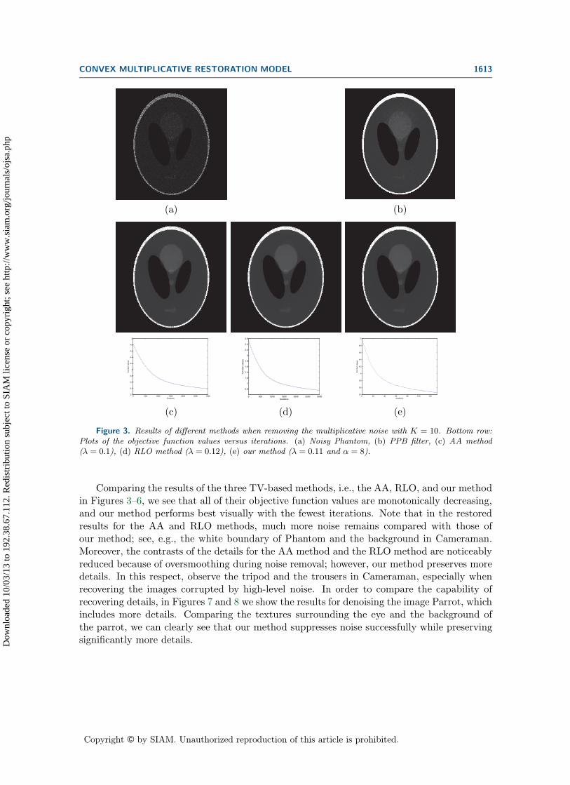
Figure 3. Results of different methods when removing the multiplicative noise with K = 10. Bottom row:Plots of the objective function values versus iterations. (a) Noisy Phantom, (b) PPB filter, (c) AA method(λ = 0.1), (d) RLO method (λ = 0.12), (e) our method (λ = 0.11 and α = 8).

Comparing the results of the three TV-based methods, i.e., the AA, RLO, and our methodin Figures 3–6, we see that all of their objective function values are monotonically decreasing,and our method performs best visually with the fewest iterations. Note that in the restoredresults for the AA and RLO methods, much more noise remains compared with those ofour method; see, e.g., the white boundary of Phantom and the background in Cameraman.Moreover, the contrasts of the details for the AA method and the RLO method are noticeablyreduced because of oversmoothing during noise removal; however, our method preserves moredetails. In this respect, observe the tripod and the trousers in Cameraman, especially whenrecovering the images corrupted by high-level noise. In order to compare the capability ofrecovering details, in Figures 7 and 8 we show the results for denoising the image Parrot, whichincludes more details. Comparing the textures surrounding the eye and the background ofthe parrot, we can clearly see that our method suppresses noise successfully while preservingsignificantly more details.D

ownl

oade

d 10

/03/

13 to

192

.38.

67.1

12. R

edis

trib

utio

n su

bjec

t to

SIA

M li

cens

e or

cop

yrig

ht; s

ee h

ttp://

ww

w.s

iam

.org

/jour

nals

/ojs

a.ph

p



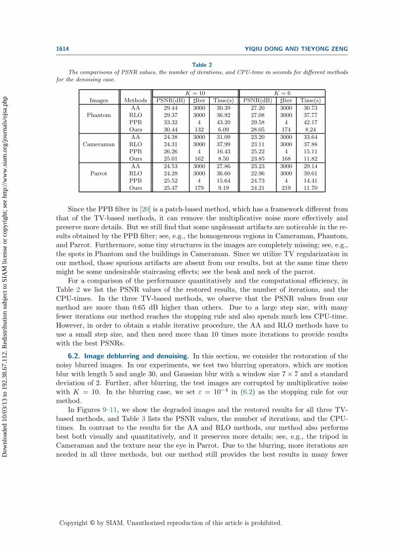
Table 2The comparisons of PSNR values, the number of iterations, and CPU-time in seconds for different methods

for the denoising case.

K = 10 K = 6Images Methods PSNR(dB) �Iter Time(s) PSNR(dB) �Iter Time(s)

AA 29.44 3000 30.39 27.20 3000 30.73Phantom RLO 29.37 3000 36.92 27.08 3000 37.77

PPB 33.32 4 43.20 29.58 4 42.17Ours 30.44 132 6.09 28.05 174 8.24

AA 24.38 3000 31.09 23.20 3000 33.64Cameraman RLO 24.31 3000 37.99 23.11 3000 37.88

PPB 26.26 4 16.43 25.22 4 15.11Ours 25.01 162 8.50 23.85 168 11.82

AA 24.53 3000 27.86 23.23 3000 29.14Parrot RLO 24.28 3000 36.60 22.96 3000 39.61

PPB 25.52 4 15.64 24.73 4 14.41Ours 25.47 179 9.19 24.21 219 11.70

Since the PPB filter in [20] is a patch-based method, which has a framework different fromthat of the TV-based methods, it can remove the multiplicative noise more effectively andpreserve more details. But we still find that some unpleasant artifacts are noticeable in the re-sults obtained by the PPB filter; see, e.g., the homogeneous regions in Cameraman, Phantom,and Parrot. Furthermore, some tiny structures in the images are completely missing; see, e.g.,the spots in Phantom and the buildings in Cameraman. Since we utilize TV regularization inour method, those spurious artifacts are absent from our results, but at the same time theremight be some undesirable staircasing effects; see the beak and neck of the parrot.

For a comparison of the performance quantitatively and the computational efficiency, inTable 2 we list the PSNR values of the restored results, the number of iterations, and theCPU-times. In the three TV-based methods, we observe that the PSNR values from ourmethod are more than 0.65 dB higher than others. Due to a large step size, with manyfewer iterations our method reaches the stopping rule and also spends much less CPU-time.However, in order to obtain a stable iterative procedure, the AA and RLO methods have touse a small step size, and then need more than 10 times more iterations to provide resultswith the best PSNRs.

6.2. Image deblurring and denoising. In this section, we consider the restoration of thenoisy blurred images. In our experiments, we test two blurring operators, which are motionblur with length 5 and angle 30, and Gaussian blur with a window size 7× 7 and a standarddeviation of 2. Further, after blurring, the test images are corrupted by multiplicative noisewith K = 10. In the blurring case, we set ε = 10−4 in (6.2) as the stopping rule for ourmethod.

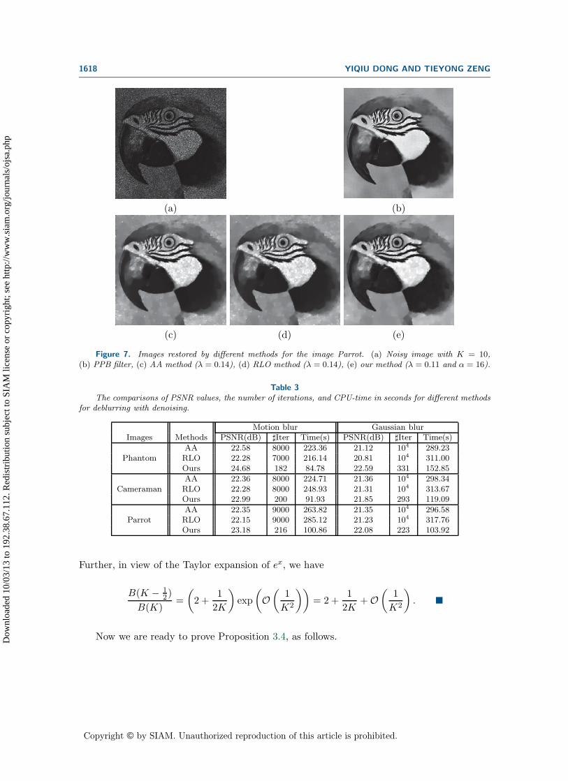
In Figures 9–11, we show the degraded images and the restored results for all three TV-based methods, and Table 3 lists the PSNR values, the number of iterations, and the CPU-times. In contrast to the results for the AA and RLO methods, our method also performsbest both visually and quantitatively, and it preserves more details; see, e.g., the tripod inCameraman and the texture near the eye in Parrot. Due to the blurring, more iterations areneeded in all three methods, but our method still provides the best results in many fewerD

ownl

oade

d 10

/03/

13 to

192

.38.

67.1

12. R

edis

trib

utio

n su

bjec

t to

SIA

M li

cens

e or

cop

yrig

ht; s

ee h

ttp://

ww

w.s

iam

.org

/jour

nals

/ojs

a.ph

p



(a) (b)

0 500 1000 1500 2000 2500 30006

7

8

9

10

11

12

13

14

15

16

iterations

func

tion

valu

es

(c)

0 500 1000 1500 2000 2500 30001

2

3

4

5

6

7

8

9

10

iterations

func

tion

valu

es

(d)

0 20 40 60 80 100 120 140 1606

7

8

9

10

11

12

13

14

iterations

func

tion

valu

es

(e)

Figure 4. Results of different methods when removing the multiplicative noise with K = 10. Bottom row:Plots of the objective function values versus iterations. (a) Noisy Cameraman, (b) PPB filter, (c) AA method(λ = 0.14), (d) RLO method (λ = 0.14), (e) our method (λ = 0.12 and α = 16).

iterations with the least CPU-times. In conclusion, our method turns out to be more efficientand outperforms the other methods which are able to deblur while removing multiplicativenoise simultaneously.

7. Conclusion. In this paper, we propose a new variational model for restoring blurredimages subject to multiplicative Gamma noise. In order to obtain the convexity, we add aquadratic penalty term according to the statistical properties of the multiplicative Gammanoise in the model proposed in [5], which combines an MAP estimator with the TV regulariza-tion. The existence and uniqueness of a solution to the new model are obtained. Furthermore,some other properties are studied, such as the minimum-maximum principle, bias correction,and so on. Due to the convexity, we are allowed to employ the primal-dual algorithm proposedin [15] to solve the corresponding minimization problem in the new model, and its convergenceis guaranteed. Compared to other recently proposed methods, our method appears to be verycompetitive with respect to image restoration capabilities and CPU-time consumption.D

ownl

oade

d 10

/03/

13 to

192

.38.

67.1

12. R

edis

trib

utio

n su

bjec

t to

SIA

M li

cens

e or

cop

yrig

ht; s

ee h

ttp://

ww

w.s

iam

.org

/jour

nals

/ojs

a.ph

p



(a) (b)

0 500 1000 1500 2000 2500 30003.5

4

4.5

5

5.5

6

6.5

iterations

func

tion

valu

es

(c)

0 500 1000 1500 2000 2500 30000.5

1

1.5

2

2.5

3

3.5

4

iterations

func

tion

valu

es

(d)

0 20 40 60 80 100 120 140 1603

3.5

4

4.5

5

5.5

iterations

func

tion

valu

es

(e)

Figure 5. Results of different methods when removing the multiplicative noise with K = 6. Bottom row:Plots of the objective function values versus iterations. (a) Noisy Phantom, (b) PPB filter, (c) AA method(λ = 0.13), (d) RLO method ( λ = 0.13), (e) our method (λ = 0.11 and α = 4).

8. Appendix I: Proof of Proposition 3.4. In order to prove Proposition 3.4, we need thefollowing lemma.

Lemma 8.1. Let B(K) denote the Beta-function B(K,K) with K ≥ 1, i.e., B(K) := Γ2(K)Γ(2K) .

Then, we have

(8.1)B(K − 1

2)

B(K)= 2 +

1

2K+O

(1

K2

).

Proof. Based on a property of the Gamma-function,

(8.2)Γ(x+ 1)

Γ(x)= x for x > 0,

Dow

nloa

ded

10/0

3/13

to 1

92.3

8.67

.112

. Red

istr

ibut

ion

subj

ect t

o SI

AM

lice

nse

or c

opyr

ight

; see

http

://w

ww

.sia

m.o

rg/jo

urna

ls/o

jsa.

php



(a) (b)

0 500 1000 1500 2000 2500 30006

8

10

12

14

16

18

20

22

24

iterations

func

tion

valu

es

(c)

0 500 1000 1500 2000 2500 30000

2

4

6

8

10

12

14

16

18

iterations

func

tion

valu

es

(d)

0 20 40 60 80 100 120 140 1606

8

10

12

14

16

18

20

iterations

func

tion

valu

es

(e)

Figure 6. Results of different methods when removing the multiplicative noise with K = 6. Bottom row:Plots of the objective function values versus iterations. (a) Noisy Cameraman, (b) PPB filter, (c) AA method(λ = 0.2), (d) RLO method ( λ = 0.2), (e) our method (λ = 0.16 and α = 16).

we readily obtain

log

(B(K − 1

2)

2B(K)

)= log

(K − 1

2

)+ 2

(log Γ

(K − 1

2

)− log Γ(K)

).

Then using the expansion of log Γ(x) with x > 0 in [2],

(8.3) log Γ(x) = x log x− x− 1

2log

x

2π+

1

12x+O

(1

x2

),

and the Taylor expansion of log(1 + x) for x ∈ (−1, 1), we get

log

(B(K − 1

2)

2B(K)

)= 1 + (2K − 1) log

(1− 1

2K

)+

1

12K(K − 12)

+O(

1

K2

)

= log

(2 +

1

2K

)+O

(1

K2

).

Dow

nloa

ded

10/0

3/13

to 1

92.3

8.67

.112

. Red

istr

ibut

ion

subj

ect t

o SI

AM

lice

nse

or c

opyr

ight

; see

http

://w

ww

.sia

m.o

rg/jo

urna

ls/o

jsa.

php



(a) (b)

(c) (d) (e)

Figure 7. Images restored by different methods for the image Parrot. (a) Noisy image with K = 10,(b) PPB filter, (c) AA method (λ = 0.14), (d) RLO method (λ = 0.14), (e) our method (λ = 0.11 and α = 16).

Table 3The comparisons of PSNR values, the number of iterations, and CPU-time in seconds for different methods

for deblurring with denoising.

Motion blur Gaussian blurImages Methods PSNR(dB) �Iter Time(s) PSNR(dB) �Iter Time(s)

AA 22.58 8000 223.36 21.12 104 289.23Phantom RLO 22.28 7000 216.14 20.81 104 311.00

Ours 24.68 182 84.78 22.59 331 152.85

AA 22.36 8000 224.71 21.36 104 298.34Cameraman RLO 22.28 8000 248.93 21.31 104 313.67

Ours 22.99 200 91.93 21.85 293 119.09

AA 22.35 9000 263.82 21.35 104 296.58Parrot RLO 22.15 9000 285.12 21.23 104 317.76

Ours 23.18 216 100.86 22.08 223 103.92

Further, in view of the Taylor expansion of ex, we have

B(K − 12)

B(K)=

(2 +

1

2K

)exp

(O(

1

K2

))= 2 +

1

2K+O

(1

K2

).

Now we are ready to prove Proposition 3.4, as follows.Dow

nloa

ded

10/0

3/13

to 1

92.3

8.67

.112

. Red

istr

ibut

ion

subj

ect t

o SI

AM

lice

nse

or c

opyr

ight

; see

http

://w

ww

.sia

m.o

rg/jo

urna

ls/o

jsa.

php



(a) (b)

(c) (d) (e)

Figure 8. Images restored by different methods for the image Parrot. (a) Noisy image with K = 6, (b) PPBfilter, (c) AA method (λ = 0.18), (d) RLO method (λ = 0.18), (e) our method (λ = 0.12 and α = 8).

Proof.

(i) Based on (3.2) and θ = 1K , we have

∫ +∞

−∞pY (y) log pY (y)dy =

∫ +∞

0pY (y)

(log

2

θKΓ(K)− (2K + 1) log y − K

y2

)dy.

Let x = 1y2. Note that the mean of η equals 1; then we get

∫ +∞

−∞pY (y) log pY (y)dy =

∫ +∞

−∞pη(x)

(log

2

θKΓ(K)+

2K + 1

2log x−Kx

)dx,

= log2

θKΓ(K)+

2K + 1

2(ψ(K)− logK)−K,

= log 2− log(√KΓ(K)) +

2K + 1

2ψ(K)−K,

where we use a property of the Gamma distribution, Eη(log x) = ψ(K)− logK (The-

orem 2.1 in [33]) and recall that ψ(K) := d log Γ(K)dK is the digamma function (see [2]).D

ownl

oade

d 10

/03/

13 to

192

.38.

67.1

12. R

edis

trib

utio

n su

bjec

t to

SIA

M li

cens

e or

cop

yrig

ht; s

ee h

ttp://

ww

w.s

iam

.org

/jour

nals

/ojs

a.ph

p



(a) (b)

0 1000 2000 3000 4000 5000 6000 7000 80003

3.1

3.2

3.3

3.4

3.5

3.6

3.7

3.8

iterations

func

tion

valu

es

0 1000 2000 3000 4000 5000 6000 70000.2

0.3

0.4

0.5

0.6

0.7

0.8

0.9

1

iterations

func

tion

valu

es

0 20 40 60 80 100 120 140 160 1803

3.5

4

4.5

5

5.5

6

6.5

7

iterations

func

tion

valu

es

0 1000 2000 3000 4000 5000 6000 7000 80005.5

6

6.5

7

7.5

8

8.5

9

9.5

iterations

func

tion

valu

es

(c)

0 1000 2000 3000 4000 5000 6000 7000 80000

0.5

1

1.5

2

2.5

3

3.5

4

iterations

func

tion

valu

es

(d)

0 50 100 150 2006

7

8

9

10

11

12

iterations

func

tion

valu

es

(e)

Figure 9. Results of different methods when restoring the degraded images corrupted by motion blur andthen multiplicative noise with K = 10. Row 1: Degraded images. Rows 2 and 4: Restored images for differentmethods. Rows 3 and 5: Plots of the objective function values versus iterations. (a) Degraded Phantom,(b) degraded Cameraman, (c) AA method (row 2: λ = 0.05; row 4: λ = 0.06), (d) RLO method (row 2:λ = 0.05; row 4: λ = 0.06), (e) our method (row 2: λ = 0.09 and α = 16; row 4: λ = 0.09 and α = 16).D

ownl

oade

d 10

/03/

13 to

192

.38.

67.1

12. R

edis

trib

utio

n su

bjec

t to

SIA

M li

cens

e or

cop

yrig

ht; s

ee h

ttp://

ww

w.s

iam

.org

/jour

nals

/ojs

a.ph

p



(a) (b)

0 2000 4000 6000 8000 100003

3.05

3.1

3.15

3.2

3.25

3.3

3.35

3.4

3.45

3.5

iterations

func

tion

valu

es

0 2000 4000 6000 8000 10000

0.2

0.25

0.3

0.35

0.4

0.45

0.5

0.55

0.6

0.65

iterations

func

tion

valu

es

0 50 100 150 200 250 3003

3.5

4

4.5

5

5.5

6

iterations

func

tion

valu

es

0 2000 4000 6000 8000 100005.5

6

6.5

7

7.5

8

8.5

9

iterations

func

tion

valu

es

(c)

0 2000 4000 6000 8000 100000

0.5

1

1.5

2

2.5

3

3.5

iterations

func

tion

valu

es

(d)

0 50 100 150 200 2506

6.5

7

7.5

8

8.5

9

9.5

10

10.5

11

iterations

func

tion

valu

es

(e)

Figure 10. Results of different methods when restoring the degraded images corrupted by Gaussian blur andthen multiplicative noise with K = 10. Row 1: Degraded images. Rows 2 and 4: Restored images for differentmethods. Rows 3 and 5: Plots of the objective function values versus iterations. (a) Degraded Phantom,(b) degraded Cameraman, (c) AA method (row 2: λ = 0.03; row 4: λ = 0.05), (d) RLO method (row 2:λ = 0.03; row 4: λ = 0.05), (e) our method (row 2: λ = 0.07 and α = 16; row 4: λ = 0.07 and α = 16).D

ownl

oade

d 10

/03/

13 to

192

.38.

67.1

12. R

edis

trib

utio

n su

bjec

t to

SIA

M li

cens

e or

cop

yrig

ht; s

ee h

ttp://

ww

w.s

iam

.org

/jour

nals

/ojs

a.ph

p



(a) (b)

(c) (d) (e)

Figure 11. Results for different methods for the image Parrot blurred by different kernels and then corruptedby multiplicative noise with K = 10 (row 2: by motion blur; row 3: by Gaussian blur). (a) Image degraded bymotion blur, (b) image degraded by Gaussian blur, (c) AA method (row 2: λ = 0.05; row 3: λ = 0.04), (d) RLOmethod (row 2: λ = 0.05; row 3: λ = 0.04), (e) our method (row 2: λ = 0.08 and α = 16; row 3: λ = 0.07 andα = 16).

(ii) Based on the PDFs of Y and the Gaussian distribution N (μK , σ2K), we have∫ +∞

−∞pY (y) log pN (μK ,σ2

K)(y)dy

=

∫ +∞

−∞pY (y) log

(1√

2πσKe− (y−μK)2

2σ2K

)dy

= −∫ +∞

−∞pY (y)

(log(

√2πσK) +

(y − μK)2

2σ2K

)dy

= − log(√2πσK)

∫ +∞

−∞pY (y)dy − 1

2σ2K

∫ +∞

−∞pY (y)(y − μK)2dy

= −1

2log(2πeσ2K),

Dow

nloa

ded

10/0

3/13

to 1

92.3

8.67

.112

. Red

istr

ibut

ion

subj

ect t

o SI

AM

lice

nse

or c

opyr

ight

; see

http

://w

ww

.sia

m.o

rg/jo

urna

ls/o

jsa.

php



where we have utilized the definition of the variance, i.e.,∫ ∞

−∞pY (y)(y − μK)2dy = σ2K .

(iii) In view of the results in (i) and (ii), using the approximation of ψ(x) in [2],

ψ(x) = log x− 1

2x+O

(1

x2

),

we have

DKL(Y ||N (μK , σ2K)) = log 2− log(

√KΓ(K))(8.4)

+2K + 1

2ψ(K)−K +

1

2log(2πeσ2K)

= log 2− log(√KΓ(K)) +

2K + 1

2

(logK − 1

2K

)

− K +1

2log(2πeσ2K) +O

(1

K

)

= log 2 +1

2logKσ2K +O

(1

K

).

Here, we obtain (8.4) by simplifying DKL(Y ||N (μK , σ2K)) with (8.3).

Moreover, based on the results in Proposition 3.1, we have

σ2K = E(Y 2)− E2(Y )

=KΓ(K − 1)

Γ(K)− KΓ2(K − 1

2)

Γ2(K)

=K

K − 1− K

2K − 1

Γ2(K − 12)

Γ(2K − 1)

Γ(2K)

Γ2(K)

=K

2K − 1− K

2K − 1

B(K − 12 )

B(K).(8.5)

Substituting the result (8.5) into (8.4) and applying the expansion in Lemma 8.1, weget

DKL(Y ||N (μK , σ2K))

= log 2 +1

2log

(K2

K − 1− K2

2K − 1

(2 +

1

2K+O

(1

K2

)))+O

(1

K

)

= log 2 +1

2log

(1

4+O

(1

K

))+O

(1

K

)

= O(

1

K

),

which yield the assertion.

Dow

nloa

ded

10/0

3/13

to 1

92.3

8.67

.112

. Red

istr

ibut

ion

subj

ect t

o SI

AM

lice

nse

or c

opyr

ight

; see

http

://w

ww

.sia

m.o

rg/jo

urna

ls/o

jsa.

php



Acknowledgment. The authors would like to thank the reviewers for the careful readingof the manuscript and the insightful and constructive comments.

REFERENCES

[1] C. Deledalle, Probabilistic patch-based filter (PPB), image analysis software, http://www.math.u-bordeaux1.fr/∼cdeledal/ppb.php.

[2] M. Abramowitz and I. Stegun, Handbook of Mathematical Functions with Formulas, Graphs, andMathematical Tables, 7th ed., Appl. Math. Ser. 55, National Bureau of Standards, Gaithersburg,MD, 1968.

[3] L. Ambrosio, N. Fusco, and D. Pallara, Functions of Bounded Variation and Free DiscontinuityProblem, Oxford University Press, London, 2000.

[4] G. Andrews, R. Askey, and R. Roy, Special Functions, Cambridge University Press, Cambridge, UK,2001.

[5] G. Aubert and J.-F. Aujol, A variational approach to removing multiplicative noise, SIAM J. Appl.Math., 68 (2008), pp. 925–946.

[6] G. Aubert and P. Kornprobst, Mathematical Problems in Image Processing. Partial Differential Equa-tions and the Calculus of Variations, Appl. Math. Sci. 147, Springer, New York, 2006.

[7] P. Bickel and K. Doksum, Mathematical Statistics: Basic Ideas and Selected Topics, Vol. 1, 2nd ed.,Pearson, NJ, 2007.

[8] J. Bioucas-Dias and M. Figueiredo, Total variation restoration of speckled images using a split-Bregman algorithm, in Proceedings of the IEEE International Conference on Image Processing, 2009,pp. 3717–3720.

[9] J. Bioucas-Dias and M. Figueiredo, Multiplicative noise removal using variable splitting and con-strained optimization, IEEE Trans. Image Process., 19 (2010), pp. 1720–1730.

[10] A. Bovik, Handbook of Image and Video Processing, Academic Press, New York, 2000.[11] S. Boyd, N. Parikh, E. Chu, B. Peleato, and J. Eckstein, Distributed optimization and statistical

learning via the alternating direction method of multipliers, Found. and Trends Mach. Learning, 3(2010), pp. 1–122.

[12] J. Cai, R. Chan, and Z. Shen, A framelet-based image inpainting algorithm, Appl. Comput. Harmon.Anal., 24 (2008), pp. 131–149.

[13] A. Chambolle, An algorithm for total variation minimization and application, J. Math. Imaging Vis.,20 (2004), pp. 89–97.

[14] A. Chambolle and P. Lions, Image recovery via total variation minimization and related problems,Numer. Math., 76 (1997), pp. 167–188.

[15] A. Chambolle and T. Pock, A first-order primal-dual algorithm for convex problems with applicationsto imaging, J. Math. Imaging Vis., 40 (2011), pp. 120–145.

[16] T. F. Chan and J. Shen, Image Processing and Analysis: Variational, PDE, Wavelet, and StochasticMethods, SIAM, Philadelphia, 2005.

[17] T. Chartrand and T. Asaki, A variational approach to reconstructing images corrupted by Poissonnoise, J. Math. Imaging Vis., 27 (2007), pp. 257–263.

[18] C. Chaux, J.-C. Pesquet, and N. Pustelnik, Nested iterative algorithms for convex constrained imagerecovery problems, SIAM J. Imaging Sci., 2 (2009), pp. 730–762.

[19] P. Combettes and J. Pesquet, A Douglas-Rachford splitting approach to nonsmooth convex variationalsignal recovery, IEEE J. Selected Topics Signal Process., 1 (2007), pp. 564–574.

[20] C.-A. Deledalle, L. Denis, and F. Tupin, Iterative weighted maximum likelihood denoising withprobabilistic patch-based weights, IEEE Trans. Image Process., 18 (2009), pp. 2661–2672.

[21] Y. Dong, M. Hintermuller, and M. Neri, An efficient primal-dual method for L1TV image restora-tion, SIAM J. Imaging Sci., 2 (2009), pp. 1168–1189.

[22] S. Durand, J. Fadili, and M. Nikolova, Multiplicative noise removal using L1 fidelity on framecoefficients, J. Math. Imaging Vis., 36 (2010), pp. 201–226.

[23] J. Einmahl, Poisson and Gaussian approximation of weighted local empirical processes, Stochastic Pro-cess Appl., 70 (1997), pp. 31–58.D

ownl

oade

d 10

/03/

13 to

192

.38.

67.1

12. R

edis

trib

utio

n su

bjec

t to

SIA

M li

cens

e or

cop

yrig

ht; s

ee h

ttp://

ww

w.s

iam

.org

/jour

nals

/ojs

a.ph

p

http://www.math.u-bordeaux1.fr/~cdeledal/\penalty \z@ ppb.php

http://www.math.u-bordeaux1.fr/~cdeledal/\penalty \z@ ppb.php



[24] E. Esser, X. Zhang, and T. F. Chan, A general framework for a class of first order primal-dualalgorithms for convex optimization in imaging science, SIAM J. Imaging Sci., 3 (2010), pp. 1015–1046.

[25] M. Figueiredo and J. Bioucas-Dias, Restoration of Poissonian images using alternating directionoptimization, IEEE Trans. Image Process., 19 (2010), pp. 3133–3145.

[26] G. Gilboa and S. Osher, Nonlocal operators with applications to image processing, Multiscale Model.Simul., 7 (2008), pp. 1005–1028.

[27] E. Giusti, Minimal Surfaces and Functions of Bounded Variation, Birkhauser Boston, Cambridge, MA,1984.

[28] T. Goldstein and S. Osher, The split Bregman algorithm for L1-regularized problems, SIAM J. ImagingSci., 2 (2009), pp. 323–343.

[29] G. Grimmett and D. Welsh, Probability: An Introduction, Oxford Science Publications, London, 1986.[30] J. Hadamard, Sur les problemes aux derivees partielles et leur signification physique, Princeton Univ.

Bull., 13 (1902), pp. 49–52.[31] Y. Huang, L. Moisan, M. Ng, and T. Zeng, Multiplicative noise removal via a learned dictionary,

IEEE Trans. Image Process., 21 (2012), pp. 4534–4543.[32] Y.-M. Huang, M. K. Ng, and Y.-W. Wen, A new total variation method for multiplicative noise

removal, SIAM J. Imaging Sci., 2 (2009), pp. 20–40.[33] M. Khodabin and A. Ahmadabadi, Some properties of generalized gamma distribution, Math. Sci., 4

(2010), pp. 9–28.[34] P. Kornprobst, R. Deriche, and G. Aubert, Image sequence analysis via partial differential equations,

J. Math. Imaging Vis., 11 (1999), pp. 5–26.[35] T. Le, R. Chartrand, and T. Asaki, A variational approach to reconstructing images corrupted by

Poisson noise, J. Math. Imaging Vis., 27 (2007), pp. 257–263.[36] F. Li, M. K. Ng, and C. Shen, Multiplicative noise removal with spatially varying regularization pa-

rameters, SIAM J. Imaging Sci., 3 (2010), pp. 1–20.[37] T. Pock, D. Cremers, H. Bischof, and A. Chambolle, An algorithm for minimizing the Mumford-

Shah functional, in Proceedings of the 12th IEEE International Conference on Computer Vision, 2009,pp. 1133–1140.

[38] B. Quinn and H. MacGillivray, Normal approximations to discrete unimodal distributions, J. Appl.Probab., 23 (1986), pp. 1013–1018.

[39] L. Rudin, P. Lions, and S. Osher, Multiplicative denoising and deblurring: Theory and algorithms, inGeometric Level Set Methods in Imaging, Vision, and Graphics, S. Osher and N. Paragios, Springer,New York, 2003, pp. 103–119.

[40] L. Rudin, S. Osher, and E. Fatemi, Nonlinear total variation based noise removal algorithms, Phys. D,60 (1992), pp. 259–268.

[41] J. Shi and S. Osher, A nonlinear inverse scale space method for a convex multiplicative noise model,SIAM J. Imaging Sci., 1 (2008), pp. 294–321.

[42] G. Steidl and T. Teuber, Removing multiplicative noise by Douglas-Rachford splitting methods, J.Math. Imaging Vis., 36 (2010), pp. 168–184.

[43] T. Teuber and A. Lang, Nonlocal filters for removing multiplicative noise, in Scale Space and Varia-tional Methods in Computer Vision 6667, Springer, New York, 2011, pp. 50–61.

[44] Y. Xiao, T. Zeng, J. Yu, and M. Ng, Restoration of images corrupted by mixed Gaussian-impulsenoise via l1-l0 minimization, Pattern Recognition, 44 (2011), pp. 1708–1728.

[45] T. Zeng and M. Ng, On the total variation dictionary model, IEEE Trans. Image Process., 19 (2010),pp. 821–825.

Dow

nloa

ded

10/0

3/13

to 1

92.3

8.67

.112

. Red

istr

ibut

ion

subj

ect t

o SI

AM

lice

nse

or c

opyr

ight

; see

http

://w

ww

.sia

m.o

rg/jo

urna

ls/o

jsa.

php

a convex variational model for restoring blurred images with multiplicative noise

Documents