A D-A 246 929Oj

STOCHASTIC VERSIONS OF THE EM ALGORITHM

by

Jean-Claude BiscaratGilles CeleuxJean Diebolt

TECHNICAL REPORT No. 227

January 1992

Department of Statistics, GN.22D uUniversity of Washington ~f C

Seattle, Washington 9819s USA 24 9*

ICI-

92- 04430

4221 5

STOCHASTIC VERSIONS OF THE EM ALGORITHM

Jean-Claude BISCARAT*, Gilles CELEUX** and Jean DIEBOLT* 1

* LSTA, 45-55, Universitd Paris VI, 4 Place Jussieu 75252 Paris Cedex, France

** lNRIA Rocquencourt 78150 Le Chesnay, France

Abstract: We compare three different stochastic versions of the EM algorithm: the SEM algorithm, theSAEM algorithm and the MCEM algorithm. We suggest that the most relevant contribution of theMCEM methodology is what we call the simulated annealing MCEM algorithm, which turns out to bevery close to SAEM. We focus particularly on the mixture of distributions problem. In this context, wereview the available theoretical results on the convergence of these algorithms and on the behavior ofSEM as the sample size tends to infinity. Finally, we illustrate these results with some Monte-Carlonumerical simulations.Keywords: Stochastic Iterative Algorithms; Incomplete Data; Maximum Likelihood Estimation;Stochastic Imputation Principle; Ergodic Markov Chain.

1. Introduction

The EM algorithm (Dempster, Laird and Rubin 1977) is a popular and often

efficient approach to maximum likelihood (ML) estimation or for locating the posterior

mode of a distribution (Tanner and Wong 1987, Green 1990 and Wei and Tanner 1990)

for incomplete data. However, despite appealing features, the EM algorithm has several

well-documented limitations: Its limiting position can strongly depend on its starting

position, its rate of convergence can be painfully slow and it can provide a saddle point of

the likelihood function (1.f.) rather than a local maximum. Moreover, in certain situations,

the maximization step of EM is untractable.

Several authors have proposed various nonstochastic improvements on the EM

algorithm (e.g., Louis 1982, Meilijson 1989, Nychka 1990, Silverman, Jones, Wilson

and Nychka 1990, Green 1990). However, none of these improvements resulted in a

completely satisfactory version of EM. The basic motivation of each of the three

stochastic versions of the EM algorithm that we study in the present paper is to overcome

the above-mentioned limitations of EM. These stochastic versions of EM are the SEM

algorithm (Broniatowski, Celeux and Diebolt, 1983 and Celeux and Diebolt, 1985), the

SAEM algorithm (Celeux and Diebolt, 1989) and the MCEM algorithm (Wei and Tanner,

1990 and Tanner, 1991). The purpose of the present paper is to compare the

I This paper has been prepared while the third author was a Visiting Scholar at the University ofWashington, Seattle. He was supported by a NATO grant, the CNRS and the ONR Contract N-00014-91-J-1074

characteristics of these stochastic versions of EM and to focus on the relationships

between MCEM and the two other algorithms.

The motivations of the introduction of a simulation step making use of

pseudorandom draws at each iteration are not the same for SEM and MCEM (SAEM is

but a variant of SEM). On one hand, the simulation step of SEM relies on the Stochastic

Imputation Principle (SIP): Generate pseudo-completed samples by drawing potential

unobserved samples from their conditional density given the observed data, for the

current fit of the parameter. On the other hand, MCEM replaces analytic computation of

the conditional expectation of the log-likelihood of the complete data given the

observations by a Monte-Carlo approximation. However, despite different motivations,

both SEM-SAEM and MCEM can be considered as random perturbations of the discrete-

time dynamical system generated by EM. This is the reason of their successful behavior:First, the random perturbations prevent these algorithms from staying near the unstable or

hyperbolic fixed points of EM, as well as from its nonsignificant stable fixed points.

Moreover, the underlying EM dynamics helps them finding good estimates of the

parameter in a comparatively small number of iterations. Finally, the statistical

considerations directing the simulation step of these algorithms lead to a proper data-

driven scaling of the random perturbations. In Section 2, we present each of these three

algorithms in the same general setting, the ideas which underlie them and their keyproperties. In Section 3, we show how these algorithms apply to the mixture problem.

Given some reference measure, a density f(y) is a finite mixture of densities from someparametrized family 3 { p(x,a): a e Al if f(y)

Kf(y) = I pk (p(y, ak), (1.1)

k=1

for some finite integer K, where the weights pk are in (0, 1) and sum to one. The mixture

problem consists in identifying the weighting parameters p, .... , PK and the parameters

al, ... , aK of the component densities, on the basis of a sample of i.i.d. observations yl,

.... YN issued from (1.1). The mixture problem and its variants and extensions is amongthe most relevant areas of application of the EM methodology (Redner and Walker 1984,

Titterington, Smith and Makov 1985). In the same section, the main results concerning

the convergence properties of the algorithms EM, SEM, SAEM and MCEM in the

mixture context are reviewed. Moreover, a theorem about the asymptotic behavior of

SEM in a particular mixture setting as the sample size goes to infinity is stated. Also, a

theorem about the almost sure (a.s.) convergence of a simulated annealing type version of

the MCEM algorithm (abbreviated s.a. MCEM hereafter) is stated. None of the proofs of

these various results is given in this paper, since each of them is very technical and the

purpose is rather to provide a brief comparative study. However, detailed references are

given for interested readers. Some illustrative numerical Monte-Carlo experiments are

presented in Section 4.2

2. The EM algorithm and its stochastic versions

2.1. The EM algorithm. The EM algorithm (Dempster et al. 1977) is an iterative

procedure designed to find ML estimates in the context of parametric models where the

observed data can be viewed as incomplete. In this subsection, we briefly review the

main features of EM. The observed data y are supposed to be issued from the density

g(ylO) with respect to some o-finite measure that we denote dy. Our objective is toA

estimate 0 by 0 = arg max L(0), where L(0) = log g(yl6). The basic idea of EM is to

take advantage of the usual expressibility in a closed form of the ML estimate of the

complete data x = (y, z). Here, z denotes the unobserved (or latent) data. The EM

algorithm replaces the maximization of the unknown L.f. f(x10) of the complete data x by

successive maximizations of the conditional expectation Q(0', 0) of log f(xl0') given y

for the current fit of the parameter 0. More formally, let k(z I y, 0) = f(x I 0)/g(y I 0)

denote the conditional density of z given y with respect to some a-finite measure dz.

Then

Q(0', 0)= k(z I y, 0) log f(x I 0') dz, (2.1)

where Z denotes the sample space of the latent data z. Given the current approximation Or

to the ML estimate of the observed data, the EM iteration 0r+l = TN(er) involves two

steps: The E step computes Q (0, Or) and the M step deteimines 0r+1 = arg max0 Q (0,

or). This updating process is repeated until convergence is apparent.

The EM algorithm has the basic property that each iteration increases the 1.f., i.e.

L(0r+l) > L(61) with equality iff Q(or+1, O'r) = Q (or , or). A detailed account of

convergence properties of the sequence {orl generated by EM can be found in Dempster

et al. (1977) and Wu (1983). Under suitable regularity conditions, {or} converges to a

stationary point of L(0). But when there are several stationary points (local maxima,

minima, saddle points), it can occur that {0r } does not converge to a significant local

maximum of L(0).

In practical implementations, the EM algorithm has been observed to be extremely

slow in some (important) applications. As noted in Dempster et al. (1977), the

convergence rate of EM (at least when the initial position is not too far from the true value

of the parameter) is linear and governed by the fraction of missing information. Thus,

slow convergence generally appears when the proportion of missing information is high.

On the other hand, when the log-likelihood surface is littered with saddle points and sub-

optimal maxima, the limiting position of EM greatly depends on its initial position.

3K .l

- L-I"

2.2. The SEM algorithm. The SEM algorithm (Broniatowski, Celeux and Diebolt

1983, and Celeux and Diebolt 1985, 1987) has been designed to answer the above-

mentioned limitations of EM. The basic idea underlying SEM is to replace the

computation and maximization of Q (0, Or) by the much simpler computation of k(z I y,

Or) and simulation of an unobserved pseudosample zr, and then to update or on the basis

of the pseudocompleted sample xr = (y, zr). Thus, SEM incorporates a stochastic step (S

step) between the E and M steps. This S step is directed by the Stochastic Imputation

Principle: Generate a completed sample xr = (y, zr) by drawing zr from the conditional

density k(z I y, Or) given the observed data y, for the current fit Or of the parameter.

SEM basically tests the mutual consistency of the current guess of the parameter and of

the corresponding pseudo-completed samples. Since the updated estimate Or+1 is the ML

estimate computed on the basis of xr, an analytic expression of Or+1 as a function of xr

can be derived in a closed form in all relevant situations.

Remark 22.1. The random drawings prevent the sequence {Or } generated by SEM from

converging to the first stationary point of the log-l.f. it encounters. At each iteration, thereis a non-zero probability of accepting an updated estimate Or+] with lower likelihood

value than Or. This is the basic reason why SEM can avoid the saddle points or the

nonsignificant local maxima of the 1.f.

Remark 2.2.2. The random sequence {Or} generated by SEM does not converge

pointwise. It turns out that this sequence is a homogeneous Markov chain, which isirreducible whenever k(x I y, 0) is positive for almost every 0 and x. This condition is

satisfied in most contexts where SEM can be applied. If {Orl turns out to be ergodic,

then it converges to the unique stationary probability distribution W of this Markov chain.

Indeed, this is a situation very similar to that prevailing in the Bayesian approach, exceptthat V cannot be viewed as a posterior probability resulting from Bayes formula. Like in

the Bayesian perspective, all the information for inference on 0 is contained in the

probability distribution W: The empirical mean of V provides a point estimate of 0 and the

empirical variance matrix of q provides information on the accuracy of this point

estimate. Since the simulation step of 0 in any Bayesian sampling algorithm (see Remark

2.2.4 below) is replaced in SEM by a deterministic ML step, the variance matrix of V is

smaller than the inverse of the observed-data Fisher information matrix.

Remark 2.2.3. In some situations, the M step of the EM algorithm is not analytically

tractable (e.g. censored data from Weibull distributions, see Chauveau 1990). Since SEM

maximizes the log-l.f. of pseudocompleted, it does not involve such difficulties.

4

Remark 2.2.4. In a Bayesian perspective, the tractability of the complete data likelihood

f(y, z 1 0) is viewed as that of the posterior density of 0 given the complete data,

1(0y, Z) f(y, zIB) n() , (2.2)J f(y, z10') n (0') d0

where 7t(0) is the prior density on 0. In this context, it is natural to replace the M step of

SEM by a step of simulation of 0 from t(0ly, z). This is actually the essence of the Data

Augmentation algorithm of Tanner and Wong (1987), which can thus be considered as

the Bayesian version of SEM. Alternatively, SEM can be recovered from the Data

Augmentation algorithm by taking a suitable noninformative prior 7r(0) and replacing the

simulation step of 0 from n(Oly, z) by an imputation step where 0 is updated as

107t(01y, z)d0. See Diebolt and Robert (1991) for more details in the mixture context.

Remark 2.2.5. Since SEM can be seen as a stochastic perturbation of the EM algorithm,

it is still directed by the EM dynamics. Thus, SEM can find the most stable fixed points

of EM in a comparatively small number of iterations. The most stable a fixed point 0f of

EM is, the longest the mean sojourn time of SEM in small neighborhoods of Of is. Since

the stability of a fixed point 0f of EM is linked to the matrix (I - J¢-' Jobs) (Of), where I is

the identity matrices, and Jc(0f) and Jobs(0 f) are the complete and observed Fisher

information matrices, respectively (see, e.g., Dempster et al., 1977, and Redner andWalker, 1984), the stationary distribution V of the SEM sequence concentrates around

the stable fixed point of EM for which the information available without knowing the

missing data, JC-1 Jobs, is the largest. This is in accordance with the approach of

Windham and Cutler (1991), who base their estimate of the number of mixture

components on the smallest eigenvalue of JC-' Jobs. Also, the SIP provides a satisfactory

data-driven magnitude for the random perturbations of SEM. When the sample of

observed data is small and contains few information about the true value of the parameter

0, the variance of these random perturbations becomes large. This is natural since in such

a case no guess 0r of 0 is very likely, so that the updated Or+ l arising from the pseudo-

completed sample xr = (y, Zr) generated from k(z I y, er) is comparatively far from or

with high probability and the variance of the stationary distribution V of SEM is large.

Such an erratic behavior makes SEM difficult to handle for small sample sizes. This is the

reason why we have introduced the SAEM algorithm, described in the next Subsection.

2.3. The SAEM algorithm. The SAEM algorithm (Celeux and Diebolt 1989) is a

modification of the SEM algorithm such that convergence in distribution can be replaced5

by a.s. convergence and the possible erratic behavior of SEM for small data sets can be

attenuated without sacrificing the stochastic nature of the algorithm. This is accomplishedby making use of a sequence of positive real numbers Yr decreasing to zero, which

parallel the temperatures in Simulated Annealing (see, e.g., van Laarhoven and Arts1987). More precisely, if or is the current fit of the parameter via SAEM, the updated

approximation to 0 is

r+l (2.30r" =G( - Yr+ 0 0 r+M + 'Yr+j 0 , (2.3)

EM SEM

where 0 (resp. 0 ) is the updated approximation of 0 via EM (resp. SEM).EM SEM

Remark 2.3.1. SAEM is going from pure SEM at the beginning towards pure EM at theend. The choice of the rate of convergence to 0 of Yr is very important. Typically, a slow

rate of convergence is necessary for good performance. From a practical point of view, itis important that Yr stays near yo = 1 during the first iterations to let the algorithm avoid

suboptimal stationary values of L(0). From a theoretical point of view, we will see inSection 3 that, in the mixture context, we essentially need the assumptions that limr,,

(yr/r+l) = I and r Yr = -c to ensure the a.s. convergence of SAEM to a local maximizer

of the log-l.f. L(0) whatever the starting point.

2.4. The MCEM algorithm. The MCEM algorithm (Wei and Tanner 1990) proposes

a Monte-Carlo implementation of the E step. It replaces the computation of Q(0, or) by

that of an empirical version Qr+ 1 (0, or), based on m (m >> 1) drawings of z from

k(z I y, Or). More precisely, the r th step: ,') Generates an i.i.d. sample zr(l),..., zr(m)

from k(z Iy, Or) and (b) Updates the current approximation to Q(0, or) as1 m

Qr+1(0, or) = y . log f(y, zr(J)) 10 ). (2.4)In1=1

(c) Then, the M step provides 0r+1 = arg max0 Qr+1(0, or).

Remark 2.4.1. If m = 1, MCEM reduces to SEM.

Remark 2.4.2. If m is large, MCEM works approximatively like EM; thus it has the samedrawbacks as EM. Moreover, if m > 1, maximizing Qr+l(0, Or) can turn out to be nearly

as difficult as maximizing Q(0, 0').

6

Remark 2.43. Wei and Tanner motivated the introduction of the MCEM algortihm as an

alternative which replaces analytic computation of the integral in (2.1) by numerical

computation of a Monte-Carlo approximation to this integral. On the contrary, SEM does

not involve exact or approximate computation of Q(0, Or): the only computation involved

in its E step is that of the conditional density k(z I y, or). Moreover, its M step is

generally straightforward, since it consists in maximizing the likelihood f(y, zr 10) of the

completed sample (y, zr). Thus, in all situations where SEM works well, it should be

preferred to MCEM.

Remark 2.4.4. The discussion in Remark 2.4.3 points out that numerical integration of

(2.1) is not the real interest of MCEM. From the comments of Wei and Tanner (1990)

and Tanner (1991) about the specification of m, it turns out that the real interest of

MCEM is its simulated annealing type version, in the spirit of the SAEM algorithm.

Indeed, Wei and Tanner recommend to start with small values of m and then to increasem as or moves closer to the true maximizer of L(O). More precisely, if we select a

sequence {mr} of integers such that mo 1 and mr increases to infinity as r-+- at a

suitable rate and perform the rth iteration with m = mr, then we go from pure SEM (mo =1) to pure EM (m = -) as r.- . Since the variance of the random perturbation term then

decreases to zero, the resulting MCEM version can be viewed as a particular type ofsimulated annealing method with I/mr playing the role of the temperature. For brevity,we call this algorithm the simulated annealing MCEM algorithm (s.a. MCEM) throughout

this paper. Note that the s.a. MCEM can still be used when no tractable expression ofQ(O, or) can be derived, in contrast with SAEM.

Remark 2.4-5. Wei and Tanner established no convergencet result for MCEM or its

simulated annealing version. In Section 3, we state a theorem which ensures the a.s.convergence of the simulated annealing MCEM to a local maximizer of L(O) for suitable

sequences {mr}, under reasonable assumptions, in the mixture context. This result

shows the interest of this version of MCEM. It is proved in Biscarat (1991) and has been

derived fron' previous results (Celeux and Diebolt 1991a and Biscarat 1991) about the

convergence of SAEM.

3. A basic example: the mixture case

3.1. The incomplete data structure of mixture data. We now focus on the

mixture of distributions problem. It is one of the areas where the EM methodology has

found its most significant contributions. Many authors have studied the behavior of EM

in this context from both a practical and a theoretical point of view: e.g., Redner and

7

Walker (1984), Titterington, Smith and Makov (1985), Celeux and Diebolt (1985),

McLachlan and Basford (1989) and Titterington (1990). For simplicity, we will restrictourselves to mixtures of densities from the same exponential family (see, e.g., Redner

and Walker 1984 and Celeux and Diebolt 199 1a).

The observed i.i.d. sample y = (Yl,.... YN) is assumed to be drawn from the

mixture density

Kf(y)= I Pk p(y, ak), (3.1)

k=1

where y E Rd, the mixing weights Pk, 0 < Pk < 1, sum to one and

9p(y, a) = D(a)-1 n(y) exp{aT b(y)}, (3.2)

where a is a vector parameter of dimension s, aT denotes the transpose of a, n : Rd --.> Rand b : Rd -4 Rs are sufficiently smooth functions and D(a) is a normalizing factor. The

parameter to be estimated 0 = (PI, ..., PK-1, al, ..., aK) lies in some subset E) of RK-

1 +sK

In this context, the complete data can be written x = (y, z) = {(yi, zi), i 1,

N}, where each vector of indicator variables zi = (zij, j = 1, ..., K) is defined by zij = 1

or 0 depending on whether the ith observation yi has been drawn from the jth componentdensity (p(y, aj) or from another one. Owing to independence, k(zly, 0) can be split into

the product Hi k(zilyi, 0) where the probability vector k(zly,0) is defined by

k(zly, 0) = p(z) (p(y, a(z)) (3.3)KI Ph (p(y, ah)

h=1

with p(z) = pj and a(z) = aj iff z = (0, ..., 1, ..., 0), 1 being in the jth position. The

posterior probability that yi has been drawn from thejth component is

tj(y, 0) - p p(yi, a) (3.4)

X Ph (p(yi, ah)h=i

The log-1.f, takes the form L(O) = Yi log{Zj pj Wp(yi, aj)} and (Titterington er al. 1985)

N KQ(0', 0) = Y Y tj(yi, 0) {log p'j + log p(yi, a'j)}. (3.5)

i=I j=

8

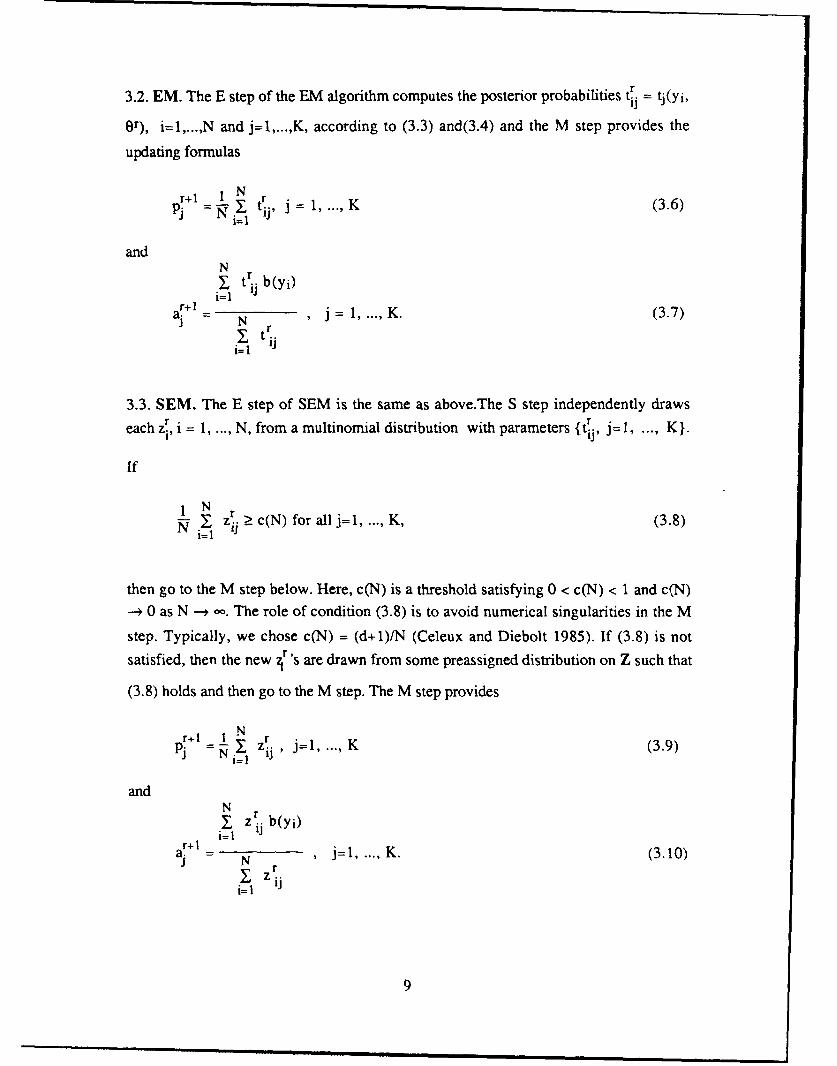
3.2. EM. The E step of the EM algorithm computes the posterior probabilities t r = tj(yi,

Or), i=l,...,N and j=l,...,K, according to (3.3) and(3.4) and the M step provides the

updating formulas

pj , j= , ... ,K (3.6)i~l

andN

tr b(yi)

aj = N r 1, K. (3.7)r+ r

i=1 j

3.3. SEM. The E step of SEM is the same as above.The S step independently drawseach zr, i = 1, ..., N, from a multinomial distribution with parameters {tJ, j=1 ... , K.

If

IN r1 X z > c(N) for all j=1, ... , K, (3.8)i=lI

then go to the M step below. Here, c(N) is a threshold satisfying 0 < c(N) < 1 and c(N)--+ 0 as N -+ -. The role of condition (3.8) is to avoid numerical singularities in the M

step. Typically, we chose c(N) = (d+l)/N (Celeux and Diebolt 1985). If (3.8) is not

satisfied, then the new r 's are drawn from some preassigned distribution on Z such that

(3.8) holds and then go to the M step. The M step provides

pi -I Z j=l, ...,K (3.9)i=1

andN

ij b(yi)i=1

a. N j=l , K. (3.10)= N ' "Sz.

i=l

i m~mmmmmm mmmIimu m m mm m m9m

3.4. SAEM. The formulas for the SAEM algorithm can be directly derived from the

above descriptions of EM and SEM and from (2.3). They are not detailed here.

3.5. MCEM. We now turn to the description of the MCEM algorithm in the mixture

case. Again, the E step is as in Subsection 3.2. The Monte-Carlo step generates mindependent samples of indicator variables zr(h)= (Zl(h), ... , zr(h)) (h 1 .... m) from

the conditional distributions {IJ j=l, ..., KI (i = 1, ..., N). Thus, from the definition of

MCEM, the updated approximation Or+ maximizes

Qr+l(O, -) = I - {log p(zr(h)) + log (p(yi, a(z (h)))} (3.11)nh=l i=l

where p(r(h)) = p and a(z!(h)) a iff zr.(h) 1. Equality (3.11) can also be writtenJ I J

N KQr+l(0, Or) = ur {log pj + log (p(yi, aj)}, (3.12)

i=1 j=l

where

# {h: h = 1, m, z.(h) = 1}ur. = m (3.13)

represents the frequency of assignment of yi to the jth mixture component, at the rth

iteration, along the m drawings. Comparing (3.5) and (3.12), it appears that MCEM justr rreplaces the posterior probabilities tJ by the frequencies ur. in the formulas (3.6) and

iii

(3.7) resulting from the M step of the EM algorithm.

Remark 3.5.1. As for SEM, the random drawings which lead to the zr(h)'s are started

afresh from a suitable distribution on Z if condition (3.8) is not satisfied.

Remark 3.5.2. As noticed above, starting with m=l and increasing m to infinity as the

iteration index grows wii produce the s.a. MCEM algorithm, quite analogous to SAEM

(see Section 3.4). Tf the s.a. MCEM is, in some sense, more elegant and natural than

SAEM, it is dramatically more time consuming than SAEM, since it involves more and

more random drawings.

3.6. Convergence properties. This subsection lists the main results concerning the

convergence properties of the algorithms examined in this paper, in the particular context10

of mixtures from some exponential family, which is the area of application of EM and its

various versions where the most precise results are available. Moreover, a result

concerning the asymptotic behavior of the stationary distribution of SEM as the sample

size N -4 0 is stated. The proofs of these results are not given in this paper, since they

are very technical.

A. Concerning EM, Redner and Walker (1984) have proved the following local

convergence result.

Theorem I (Redner and Walker 1984). - In the context of mixtures from some

exponential family, if the Fisher information matrix evaluated at the true 0 is positive and

the mixture proportions are positive, then with probability J,for N sufficiently large, the

unique strongly consistent solution ON of the likelihood equations is well defined and the

sequence {Or} generated by EM converges linearly to ON whenever the starting point 00

is sufficiently near ON.

B. Concerning SEM, Celeux and Diebolt (1986, 1991b) have proved the ergodicity of

the sequence {0r} generated by SEM in the mixture context. The proof reduces to

showing that the sequence {zr} is a finite-state homogeneous irreducible and aperiodic

Markov chain. This result guarantees weak convergence of the distribution of or to the

unique stationary distribution XN of the ergodic Markov chain generated by SEM. (The

index N indicates dependence on the sample.) However, such a result does not guarantee

that NWN is concentrated around the consistent ML estimator ON of 0 mentioned in

Theorem 1. Celeux and Diebolt (1986, 199 1b) have examined the asymptotic behavior of

W4N. They start by showing that the SEM sequence satifies a recursive relation of the form

0r1 = TN(Or) + VN(Or, Zr), (3.14)

where TN denotes the EM operator and VN : Rs x Z -* Rs is a measurable function such

that -N VN(Or, Zr) converges in distribution as N -) o, uniformly in 0 e GN (compact

subset of 8), to some Gaussian r.v. with mean 0 and positive variance matrix. In the

particular case of a two-component mixture where the the mixing proportion p is the only

unknown parameter, they have established the following result.

Theorem 2 (Celeux and Diebolt (1986, 1991b)). - Let f(x I p) = p'pl(x) + (I - p)p2(x), 0

< p < 1. be the density with respect to some a-finite measure li(dx) of a two-component

mixture where the densities p I and (P2 are assumed known. Then, for a suitable rate of

convergence to 0 of the threshold c(N) introduced in (3.8):

11

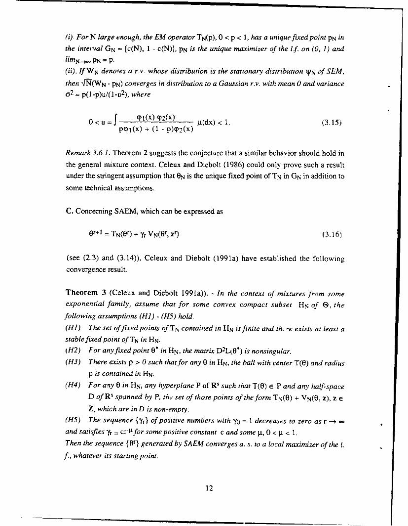
(i). For N large enough, the EM operator TN(p), 0 < p < 1, has a unique fixed point PN in

the inteival GN = [c(N), 1 - c(N)], PN is the unique maximizer of the If. on (0, 1) and

limN--, PN = P.

(ii). If WN denotes a r.v. whose distribution is the stationary distribution 1N'N of SEM,

then N(WN - PN) converges in distribution to a Gaussian r.v. with mean 0 and varianceo2 = p(1 -p)uI(1 -u2), where

0 < u f (P IW01(x)P2(x) g(dx) < 1. (3.15)p(p1(x) + (1 - P)(P2(x)

Remark 3.6.1. Theorem 2 suggests the conjecture that a similar behavior should hold in

the general mixture context. Celeux and Diebolt (1986) could only prove such a resultunder the stringent assumption that ON is the unique fixed point of TN in GN in addition to

some technical assumptions.

C. Concerning SAEM, which can be expressed as

0r+1 = TN(Or) + Yr VN(0 r , zr) (3.16)

(see (2.3) and (3.14)), Celeux and Diebolt (1991a) have established the following

convergence result.

Theorem 3 (Celeux and Diebolt 1991a)). - In the context of mixtures from some

exponential family, assume that for some convex compact subset HN of E, the

following assumptions (HI) - (H5) hold.

(HI) The set of fixed points of TN contained in HN is finite and th, -e exists at least a

stable fixed point of TN in HN.(H2) For any fixed point 0* in HN, the matrix D2L(0*) is nonsingular.

(H3) There exists p > 0 such that for any 0 in HN, the ball with center T(0) and radius

p is contained in HN.

(H4) For any 0 in HN, any hyperplane P of Rs such that T(0) r P and any half-space

D of Rs spanned by P, the set of those points of the form TN(0) + VN(0, z), z

Z, which are in D is non-empty.

(H5) The sequence {yr} of positive numbers with y0 = 1 decreaes to zero as r -4

and satisfies yr = cr-4for some positive constant c and some .t, 0 < t < 1.

Then the sequence {Or} generated by SAEM converges a. s. to a local maximizer of the 1.

f, whatever its starting point.

12

Remark 3.6.2. For EM, the possibility of convergence to a saddle point of the L.f. is

always present. On the contrary, Theorem 3 ensures that SAEM does not c.,averge to

such a point a.s. The basic reason why SAEM achieves better results than EM is that

SAEM does not necessarily terminate in the first local maximum encountered.

Remark 3.6.3. The assumption (H4) is very technical, but is reasonable for N large

enough, since the number of points of the form TN(O) + VN(O, z), z r Z, is equal to KN.

D. Concerning the s.a. MCEM algorithm, which can be expressed as

or+l = TN(0r) + U (3.17)

where jr {zr(h), h=l,..., m(r)} represents the vector of the m(r) samples drawn at

iteration r and UrN : Rs x Zm(r)-- Rs is a measurable function, Biscarat (1991) has

established the following convergence result.

Theorem 4 (Biscarat 1991). - In the context of mixtures from some exponential family,

assume that for some convex compact subset HN of 8, the above assumptions (HI) -

(H.3) hold along with the following assumption (1-15 bis):

(H5 bis). There exists a positive constant aF such that ra = o{m(r)} (r--->o).

Then the sequence {Or} generated by the s.a. MCEM algorithm converges a. s. to a local

maximizer of the 1. f., whatever its starting point.

Remark 3.6.4. Theorem 4 does not require the technical assumption (1-14). This is

essentially due to the fact that the noise Ur is asymptotically Gaussian as r -4 . In this

perspective, MCEM can be thought of as more natural than SAEM.

6. Numerical comparisons of EM, SEM, SAEM and MCEM

In this section, we compare the practical behavior of EM, SEM, SAEM and

MCEM on the basis of a Monte-Carlo experiment in a small sample context for a

Caussian mixture which is somewhat difficult to identify. For each sample size N = 100

and N = 60, we gene.ated 50 samples from an univariate four-component Gaussian

mixture with weights pi = p2 = P3 = p4 = 0.25, means ml = 2, m2 = 5, m3 =9 and m42 2 2 2=4.Frehgerad=15 and variances 02 = 0.625, 02 = 0.25, 03 = I and o2 4. For each generated

sample, we performed 200 iterations of EM, SEM and SAEM using two different

13

initialization schemes. In the first one, we started from the true parameter values. In the

second one, the initial positions of the parameters were drawn at random as follows. We

first drew uniformly four points cl, ... , c4 among {Y1, ..., YNI. We then partitioned the

sample into four clusters by aggregating each yi, i = 1, ..., N, around the nearest of cl,

c4. Finally, we computed the initial parameters on the basis of these four clusters.

In order to derive in a simple way, from the SEM scheme, a reliable pointwise

estimate of the mixture parameters, we used a hybrid algorithm. We ran 200 SEMiterations. Then we ran 10 additional EM iterations starting from the position which

achieved the largest value of the likelihood function among these 200 SEM iterations.The choice of the rate of convergence to 0 of the sequence {yr} for SAEM is very

important and delicate. From our experience, the following cooling schedule turns out togive good results yr = cos rcx for 0 < r < 20, and Yr = c/ rF for 21 < r < 200, where cos(20 x) = c / -- 0= 0.3. We performed the s.a. MCEM algorithm with mr = [1/y r ] and Yr

as above to have the same cooling rate for SAEM and s.a. MCEM, in view of (3.16) and(3.17). Moreover, in these numerical experiments, we did not take into account the trialsfor which one of the mixing weights pj (j = 1, 4; r = 1, ..., 200) became smaller than

2/N. This procedure ensures that (3.8) holds with c(N) = 2/N.The results obtained when starting from the true parameter values are not reported

here. For both sample sizes, the four algorithms gave similar satisfactory estimates.Therefore, when strong prior information on the parameters is available, EM should bepreferred to its stochastic variants even for small sizes, because of its simplicity.

The results corresponding to random initial positions are displayed in Table 1. In

this table, the first row indicates the algorithm which has been performed. The secondrow indicates the sample size. The row '#' provides the number of successful trials (outof 50). Then, the rows 'PI' - 'P4', 'mi' - ' 4 ' and ' 2, v 2,'~~ ~ "4 l provide the average and

standard deviation, into brackets, of the estimates of these parameters over the '#'recorded trials.

Table I about here

These results highlight the main practical differences between EM and the three

stochastic versions of EM under consideration.Since the samples were small, the likelihood functions were littered with many

local maxima, and the EM algorithm provided solutions which greatly depended on its

initial positions. This is apparent from the mean values of the first two component

parameters, which are far from the true values, and from the large standard deviations of

the estimates.

14

These simulations illustrate the poor performance of SEM for small samples (only

17 successful trials out of 50 for N = 60 with the random initialization): This is the reason

why SAEM, which can be regarded as a simulated annealing type version of SEM, has

been proposed. However, SEM provides good results when the trials can be achieved

and other numerical experiments for moderate sample sizes highlight its ability to avoid

unstable stationary points of the likelihood (see, e.g., Celeux and Diebolt 1985).

They also show that if the temperatures in SAEM and s.a. MCEM are chosen

such that the magnitudes of the perturbations of both algorithms decrease at similar rates,

then SAEM and s.a. MCEM give very close results; furthermore, if the rates of the

temperatures are suitably chosen, then both algorithms remain more stable than SEM for

small samples and give better results than EM; however, the major drawback of s.a.MCEM is that it requires more and more pseudorandom draws as the iteration number

increases: The CPU time of each run of s.a. MCEM in our trials was about 25 times the

corresponding time for SAEM. Another drawback, common to SAEM and s.a. MCEM,is that no data-driven determination of the temperatures is available (see also the Monte-

Carlo simulations in Celeux and Diebolt, 199 la).

Acknowledgements. We are grateful to C. P. Robert and M. P. Windham for their

much valuable comments.

REFERENCES

Biscarat, J.L. (1991). "Almost Sure Convergence of a Class of Stochastic Algorithms."

Rapport Technique LSTA, Universit6 Paris 6 (to appear).

Broniatowski, M., Celeux, G. and Diebolt, J. (1983). "Reconnaissance de M6langes de

Densitts par un Algorithme d'Apprentissage Probabiliste." Data Analysis and

Informatics, 3, 359-374.

Celeux, G. and Diebolt, J. (1985). "The SEM Algorithm: a Probabilistic Teacher

Algorithm Derived from the EM Algorithm for the Mixture Problem." Computational

Statistics Quaterly, 2, 73-82.

Celeux, G. and Diebolt, J. (1989). "Une Version de type Recuit Simuld de l'Alagorithme

EM." Notes aux Comptes-Rendus de l'Acadmie des Sciences, 310, 119-124.

Celeux, G. and Diebolt, J. (1986). "Comportement Asymptotique d'un Algorithme

d'Apprentissage Probabiliste pour les Mdlanges de Lois de Probabilit6." Rapport de

recherche INRIA , 563.

Celeux, G. and Diebolt, J. (1987). "A Probabilistie Teacher Algorithm for Iterative

Maximum Likelikood Estimation." Classification and related methods of Data

Analysis. North Holland, 617-623.

15

Celeux, G. and Diebolt, J. (1991a). "A stochastic Approxiata i, Type EM Algorithm

for the Mixture Problem." Rapport de recherche INRIA , 1383.

Celeux, G. and Diebolt, J. (1991b). "Asymptotic Properties for a Stochastic EM

Algorithm for estimating mixture proportions." Technical Report, University ofWashington, Seattle.

Chauveau, D. (1991) "Algorithmes EM et SEM pour un Mdlange Cachd et Censur."

Revue de Statistique Appliquie,

Dempster, A. P., Laird, N. M. and Rubin, D. B. (1977). "Maximum Likelikood fromIncomplete Data via the EM Algorithm (with discussion)." Journal of the Royal

Statistical Society, Ser. B 39, 1-38.

Diebolt, J. and Robert, C. P. (1991). "Estimation of Finite Mixture Distribution throughBayesian Sampling."Journal of the Royal Statistical Society, Ser. B (to appear).

Green, P. J. (1990). "On Use of the EM Algorithm for Penalized LikelihoodEstimation." Journal of the Royal Statistical Society, Ser. B 52, 443-452.

van Laarhoven, P. J. M. and Aarts, E. H. L. (1987). Simulated Annealing: Theory and

Applications. Reidel: Dordrecht.Louis, T. A. (1982). "Finding the Observed Information Matrix when Using the EM

Algorithm." Journal of the Royal Statistical Society, Ser. B 44, 226-233.McLachlan, G.J. and Basford, K.E. (1989). Mixture models - Inference and applications

to Clustering, New York: Marcel Dekker.Meilijson, I. (1989). "A Fast Improvement to the EM Algorithm on its Own Terms."

Journal of the Royal Statistical Society, Ser. B 51, 127-138.Nychka, D.W. (1990). "Some Properties of Adding a Smoothing Step to the EM

Algorithm." Statistics and Probability Letters, 9, 187-193.

Redner, R.A. and Walker, H.F. (1984) "Mixtures Densities, Maximum Likelikood and

the EM Algorithm." SIAM Review, 26, 195-249.Silverman, B. W., Jones, M. C., Wilson, J. D. and Nychka, D. W. (1990). "A

Smoothed EM Approach to Indirect Estimation Problems, with Particular Reference to

Stereology and Emission Topography." Journal of the Royal Statistical Society, Ser.B 52, 271-324.

Tanner, M. A. (1991). Tools for Statistical Inference. Lectures Notes in Statistics 67,

New York: Springer-Verlag.Tanner, M. A. and Wong, W. H. (1987). "The Calculation of Posterior Distribution by

Data Augmentation (with discussion)." Journal of the American Statistical

Association, 82, 528-550.Titterington, D. M. (1990). "Some Recent Research in the Analysis of Mixture

Distribution." Statistics, 21, 619-640.

16

Titterington, D. M., Smith, A. F. M. and Makov U. E. (1985)Statistical Analysis of

Finite Mixture Distribution. New York: Wiley.Wei, G. C. G. and Tanner, M. A. (1987). "A Monte Carlo Implementation of the EM

Algorithm and the Poor Man's Data Augmentation Algorithms." Journal of the

American Statistical Association, 85, 699-704.

Windham, M. P. and Cutler, A. (1991). "Information Ratios for Validating Cluster

Analyses." Working paper, Utah State University (Logan).

Wu, C.F. (1983). "On the Convergence Properties of the EM Algorithm." Annals of

Statistics, 11, 95-103.

17

aig. EM SEM SAEM MCEM EM SEM SAEM MCEM

N 100 100 100 100 60 60 60 60

# 50 28 38 36 50 17 30 27

P, 0.28 (0.14) 0.23 (0.05) 0.24 (0.05) 0.24 (0.05) 0.32 (0.14) 0.26 (0.06) 0.25 (0.05) 0.25 (0.05)

P2 0.26 (0.10) 0.24 (0.03) 0.24 (0.04) 0.24 (0.04) 0.26 (0.12) 0.27 (0.05) 0.25 (0.07) 0.26 (0.05)

P3 0.20 (0.09) 0.28 (0.05) 0.26 (0.06) 0.27 (0.06) 0.21 (0.10) 0.23 (0.05) 0.26 (0.07) 0.27 (0.07)

P4 0.25 (0.10) 0.25 (0.05) 0.26(0.04) 0.25 (0.05) 0.22 (0.11) 0.24 (0.07) 0.25 (0.06) 0.23 (0.07)

m1 2.34 (0.70) 2.02 (0.05) 2.01 (0.05) 2.02 (0.05) 2.45 (0.76) 2.10 (0.38) 2.01 (0.06) 2,08 (0.06)

m 2 5.96 (2,10) 4.99 (0.12) 4.98 (0.12) 4.99 (0.14) 6.22 (1.96) 5.33 (1.06) 5.00 (0.14) 4.97 (0.13)

m 3 9.80 (2.31) 9.14 (0.26) 9.04 (0.23) 9.06 (0.24) 10.13 (2.53) 9.37 (1.34) 9.01 (0.29) 9.09 (0.34)

m 4 15.00 (1.29) 15.04 (0.57) 14.99 (0.51) 14.98 (0.61) 15.28 (1.44) 15.06 (0.70) 15.00 (0.65) 15.02 (0.67)

a1 0.71 (1,07) 0.07 (0.02) 0.06 (0.02) 0.07 (0.02) 0.80 (1.22) 0.20 (0.58) 0.06 (0.02) 0.07 (0.02)

a2 0.77 (1.55) 0.22 (0.08) 0.23 (0.08) 0.28 (0.10) 0.96 (1.88) 0.29 (0.20) 0.23 (0.08) 0.26 (0.12)23 1.09(1.48) 1.10(0.58) 1.08(0.76) 1.11 (0.73) 0.90(0.96) 0.79(0.46) 0.92(0.68) 0.88(0.56)

2a4 3.91 (3.25) 3.29 (1.40) 3.71 (1.67) 3.47 (1.55) 3.25 (3.00) 3.64 (2.96) 3.62 (2.33) 3.78 (2.50)

Table 1. Number of successful trials (row #), mean and standard deviation of the estimates of the

mixture parameters using EM, SEM, SAEM and MCEM, with random initializations,for the sample

sizes N = 100 and 60.

18

SECURITY .._ASSIFICATION OF 'NSPAGE (VA,.. Oio. En-ld

REPORT OCUME14TATION PAGE SFRE fOML'JSRU7NS R1. REPORT NUMBER 2. GOVT ACCESSION NO. 1 3. REC;PIE4T*S CATAL.OG NUMBER

4. TITLE (drid..,itle) 5. TYPE OF REPORT & PERIOD COVERED

Stochastic Versions of the EM Algorithm TR 10-1-90 to 9-30-93

6. PERFORMING ORG. REPORT NUMBER

7. AujTHOR(s) 0. CONTRACT OR GRANT NUM4BER(.)I

Jean-Claude BISCARATGilles CELEUX arnd-' Jean Di-ebolt N00014-91-J-1074

9. OcRORMING ORGANIZATION NAME AMC ACCRESS AREPCIAA & WGR EJNT NUMB'ERS TSffniversity of Washington ARE OKJ1 UaR

Dept of StatisticsSeattle, WA 98195

It. CONTROL..IMG OFFICE NAME ANC ADDRESS tZ. REPORT DATE

ONR Code N63374 _______________

1107 NE 45th St. 13. NUMBER OF PAGE5

Seattle- wA gins 19Is. MONI 7ORING AGENCYr NAME a ADORESS(It d~f!.,nt f1ram Controlling Office) 1S. SECURITY CL.ASS. (at ctLe report)

ISUnclasifiPH-15. EC._A5SIFICA7IOM/ DOWNGRADING

SCHEDtjL.E=

6. ZISTRIBUrION ST A7EMENT7 (at Enos R.poe;

APPRO/End FOR PUBL: C RELEASE: DISTMIBUTI "ON UNLIMITED.

'7. DIST RIBUTION ST ATEMZNT (of vt* absract oseiered In alocAt 20. if affferve, from Report)

IS. SUPPL.EMEN4TARY NOTES

19. K EY WORDS (CantIn.u. on ~toor ids It necirse~r and~ Identifty by' blak number)

Stochastic Iterative Algorithms, Incomplete Data, Maximum Likelihood Estimatifn,Stochastic Imputation Principle, Ergodic Markov Chain

20. A0!S? PACT (Contnue. an rees side It nacesear and IdenCtf by oilock rot.WIO*)

We compare three different stochastic versions of the EM algorith: the SEM al-gorithm, the SAEM algorithm and the MCEM algorithm. We suggest that the mostrelevant contribution of the MCEM emthodology is what we call the simulated an-nealing MCEM algorithm, which turns out to be very close to SAEM. We focusparticularly on the Mixture of distributions problem. In this c ontext, wereview the available theoretical results on the convergence of these algorithmsand on the behavior of SEM as the sample size tends to infinity. Finally we

DO O'RI 1473 E3ITIO. OF 1 NOV, 65 IS OS3SOLE'TE

S/ N 0 102. - 01 4- 66 1 SECURITY C:.ASSIFiCATiOM OF THIS PACE *

illustrate these results with some Monte-Carlo numerical simulations.