LU

O CO

Office of Naval Rt »earch Contract Nooar-144

Task Order II (NE 062..010)

POTE^niAL FLOW THROUGH RAÖlÄi. FLOW

TURBOMACHINE MOTORS

A. }. AcosU

Uvrfrndtrtukmics Laboratory California ln*tttute of Technology

Pasadena» California

Report No« £-19*4 r«oruary 19S4

<mmmv ,*

x

! ft - - fir i

I«»

•

t r

T able of Contents

Abstract

i. Introduction

II. Formulation of the Problem

Mapping Function

III. The Displacement Flow

Conjugation of the Displacement Flow

IV. The Through Flow

a. Pump

b. Turbine

V. Head Flow-Rate Equation

a. Pump

Calculation of Values of +0

Condition of Shockless Entry

b. Turbine

Shockless Entry

Torque Characteristics

VI. Extension to Nonlogarithmic Spiral Shapes

a. Solution for Any Power Boundary Condition

b. Application to the Through Flow

Boundary Condition for Nonlogarithmic Spiral

c. Application to the Displacement Flow

d. Head Flow-Rate Equation

e. Shockless Entry

VII. Extension to Nonradial Profiles

a. Flow Over a Conical Surface of Small Constant Breadth

b. Effect of Variation in Breadth

c. Remark on Application Mixed Flow Impellers

d. Remark on the Influence of Compressibility

e. Numerical Examples

VIII. Concluding Remarks

IX. Notation

X. References

Figures

1

1

2

3

5

6

10

10

11

12

12

14

17

19

21

21

22

23

24

25

28

30

31

33

34

35

->7

39

40

43

45

47

'

!

~ • . ' '- . v-

Abstract

X The exact theory of incompressible potential flow through pump im-

pellers with logarithmic spiral (constant angle) blades is extended to include

radial or conical turbomachines with small variations in vane angle and

passage breadth. Approximate formulas are obtained and charts given for

smooth entry and performance characteristics of pump or turbine configura-

tions when the solidity is somewhat greater than unity and when the major

blade deviations are confined to the inlet regions. However, the results of the

present analysis are general and may be applied to blade rows with reasonably

arbitrary camber lines.

1* I. Introduction

'*

In recent years there has been some attention given to the problem of

calculating the performance of compressor or pump impellers with a finite

number of blades. ' By and large these efforis consist of solving field

equations either by numerical methods (i.e. the relaxation technique) or by

variations of stream filament theories. If compressibility effects must be

considered it appears inevitable that such methods must be used, particularly

if any of the flow details, e.g., velocity distributions, are desired. Further-

more, since the impeller geometries commonly employed are rather complex

the question of analysis is made increasingly difficult. Although it is possible

to obtain velocity and pressure fields for rather arbitrary configurations by

the methods proposed in Refs. 1 and 2» the labor and time required for

solutions are prohibitive for most engineering situations. Moreover, these

calculations are for specific cases and do not permit generalizations to be

made from them.

•

•

•

;

>

** ; It was precisely Decause oi tne se limitations tnat tne earlier extorts oi 3 .. 4

Spannhake and Sorensen were devoted to obtaining analytic solutions for

impeller geometries of somewhat simplified shape. Spannhake obtained ehe

incompressible, nonviscous head flow-xate characteristic for impellers with

straight radial blaaes of arbitrary radius ratio with constant impeller breadth.

Later, Sörensen extended the theory to include the effect of constant blade or

.

i

'

-2-

stagger angle, bur. was unable to obtain exact solutions in closed form lor the

overall performance parameters. A. Busemann in 1928 finally solved this

problem and obtained expressions for the head flow-rate equation as well as

for the "shockless entry" condition. His analysis was restricted to the

potential flow in "two-dimensional" impellers with a finite number of logarith-

mic spiral blades. These result? are exact insofar as the results are given

in series which may be calculated to any accuracy desired. Busemann's

theory gives a good approximation for many cases provided the flow is pre-

dominantly radial or two-dimensional. However, most impellers are not

two-dimensional nor are the impeller blades strictly logarithmic spirals.

It is to this last problem that this present work is mainly devoted. Un-

fortunately, a truly exact general analytic solution would involve great

difficulties, so that approximations must be rriade. The program to be fol-

lowed herein consists first of obtaining a more general form of Busemann1 s

results by a slightly different method. Inasmuch as this theory is applicable

to turbines as well as pumps both sets of coefficients will be given. It will

then be seen that approximations in the spirit of the thin airfoil theory can be

made. The approximate problem is then formulated and the results are given

for . all variations in blade shape and impeller breadth. It will also be

shown that under certain conditions these results apply to (Iowa over

cones so that the present results may form the i carting point for a theory of

mixed flow impellers.

In the course of this work, approximate formulas may be obtained easily

for the case of high solidity. These have been found to be extremely useful

for a rapid estimate of the overall performance.

.-

'

II. Formulation of the Problem

*•

In this and the following three sections we work out the potential flow

through a circular array of equally spaced logarithmic spiral blades. The

breadth of the impeller is assumed to be constant. Under these conditions

the flow is two-dimensional and hence the methods of conformal mapping may

be used. An important simplification in this problem is that the flow due to

the rotation of the blades may be treated separately from the through flow,

A . .-.»•T

»W» V •'-. , ' "•=. . .,..:

'

a

-3-

i.e.j the flow responsible for net discharge through the runner. In this sec-

tion the properties of the mapping function which enable these problems to be

solved are worked out. In the succeeding aections the flow arising from the

rotation of the blades in still watei (displacement flow) and the through flow

are obtained.

Mapping Function

The mapping function is"

z = w - w

o

o

1

w - l/w

w -I

e nr

(i)

or,

dz z

e iY dw [ e1^ w L w0-l

w /w

•IV e ' w 'V - w

o (2)

It is easy to verify that £q.(l)is the desired function since when w is on the

unit circle Eq,(2) gives Arg dz/z = Y which is precisely the equation of a

logarithmic spiral. Moreover, Eq.(l)is a single valued function if |wji 1

and the point w is not enclosed. If w is enclosed, once the argument of

z increases by ZTT/N, thus moving a point in one blade passage to a congruent

ptint in the next adjacent one. Fig. la. The point w is the complex (

constant and represents the origin of the physical plane. The point w = oo

corresponds to z = oo also. This functic>. io slightly different than the one

usually used for annular or cascade flows. The end points of the blade are

given by the roots of dz/dw = 0. If the point corresponding to the exit tip of

the blade is arbitrarily chosen as unity, then

w2 . 1

\v - e i(2y + iö+ü)

and

w = a e o i6

a = sin x /sin( y + 6 )

(4)

I

I

.

where w. corresponds to the inlet edge of the blade. From the above

the exit radius of the blade r? = jz?J = 1, thus the radius ratio of the im-

peller is given as r./r? - ja.| or using Eq.(l)one obtains

1 4- cos 2Y

Lin12Yiij] sin 6 I

2( y-fi-Y).:. ?v

For straight radial blades y = 0 an(* Eq.(5) reduces to

i fa" 1

La +

2/N

From Eq. 4

(5)

(5a)

.<?

tan r = a sin 6

1-a cos 6

from which Fig. lb may be constructed. As an aid in determining the

constants a and 6 the following expressions are useful:

a2-l 2 cos2 Y

co ̂ rv-^sinYfr-e-jcn L 2 cos Y J

where

o- = N In r^/r.

COSY

In case a srf 1, the relation

(5b)

_ <r-4 siny (TT-5-Y) 2 i A 2^ 2 cos Y a - 1 = 4 cos Y e (5c)

k*

5

may be used as an approximation. Equation(5b)is plotted in Fig. 2.

I .«w ,

i. ' -5-

V

..•-*-^-- •

III. The Displacement Flow

S5e

In order that there be no flow through the surface of the blade, the

velocity component of the flow normal to the blade must satisfy the condition

V -- n • co x r

•\:.

where a is the outward normal of the blaÄe surface. Thus the normal

vector velocity must be

V = as cos Y z, e nz b i(ir/?-+Y)

Let F be the complex po*ential of this flow. Then

dF dF dz d"w d"z * d"w '

and dF/dz is the conjugate of the vector velocity V in the z-plane. Since z polar coordinates must be used in the w-plane, we have as the boundary con-

dition on the unit circle

V e rw •iO , _ dzb ~i(Tt/2+Y)

= M cos Y '% 3w" e (6a)

With the aid of Eq. (2) one obtains finally

rw co cos- w zbzb

i(Y-«) -i(Y-O)

w • *- o •TT vi - e

o r*r (6b)

where

zbzb

iO w - e

o w'-l

w - e o

-iO

«v - *.

q = i (!•.»*>

(6c)

;

The problem is now to find the corresponding tangential velocity

•

•• -: "F

* »A

1 • •

-6-

distribution on the unit circle subject to the additional restriction that this

velocity vanish at infinity. The solution may be obtained in any number of

ways. The most direct consists of writing the complex potential F in the

form oo

> A w Z_i n n=o

-n

and solving for the coefficients by means of Eq» 6b and hence obtaining the

conjugate velocity V- . The procedure that will be followed herein is

essentially the same as that outlined above and differs only in some details.

In order to effect a solution, the fact will be used that if the normal

component of the velocity about the unit circle can be written as

m i

I >•»

Vr = f(e-i0) +7(eiQ)

then the tangential velocity is

,. 1 r-7 , iOv ,/ -i0> I

(7)

provided that the velocity should vanish at infinity. This statement is essen- 7

tially a variation of Milne-Thompson's circle theorem. Thus in order to

obtain the conjugate velocity VQ all that must be done is to arrange Eq,(6b) iO in ascending and descending powers of e and then to apply Eq.(7). In

Eq. (7), V0 is frequently spoken of as the "conjugate function" or simply

the conjugate of V .

Conjugation of the Displacement Flow

Since |w \h \ , the brackets in Eq. (6b) may be expanded by the

binomial theorem. If the terms are arranged in positive and negative powers iO o.t e* one obtains for the boundary condition in the w-plane

"*•• \

jCü cos Y

N ••(-q)r(-q)

w \ -A w -1 I

o J

w o

w -V o

q f oo V P(n-q)r(n-q)

l x i . i i 2n I n=o "• ni |w0|

-T ik.9 \

w

A, e -ikQ -

— k w o

ei(Y-0)

= ^B w - e o

-i(Y-O)

w - e o (8)

! - -* t.**-3 \

7- ^ J

where oo

A. V r(m+k-q)n(rn-q) (m+k/l mi |w |

m=o ' ° 2m

The following terms must now be conjugated:

(9)

i ; . y r(n-q)r(n-q) T £l^

r.=o nl tt! tw0l L wo"e

-i(Y-O)

IT w - e o

-iY i(k+l)9 A^ eiYe-i(k+l)

1 w w - e o

e e 7=V""= ^TBT i w w - e

and

iY i(k-l)0 e <?

J3 " 1 w w - e o TTT

*k •=TT -

1 w

-iY -i(k-l)0 e i e v /

w - e o •

The terms S. and 5? are easily conjugated by a straightforward application

of Eq. (7). However, it is evident that if the denominatcr of S- is expanded

by the binomial theorem then S, will contain terms of both positive and nega- iO tive powers of e . Thus in order to accomplish the conjugation it will be

necessary to separate these terms, S, can be written as

co Ake

1 w n=.

.i(k-n}0

— n w o

+ conj. term

with the aid of the geometrical series. Now if in the first sum

4 k - n = r = 0, 1, 2 • • • for n £ k

k-n=-r=l,2, 3 • • • for n > k

then S, r»*ay be written in four separate terms as •

X w '- •w ,..

K.«

-{$•

J. I

-.1

S3 =

;r« Ave' iY k-1 •irQ

. k 1 w o r=ow0

."~k" Z_, 1Wo r^o

k-r w o

* -irO V e A. e"iY °°

lwo rT^

ir 0 e . k 1 w o

/ . k+r trzri w r-i 0

k+r w o

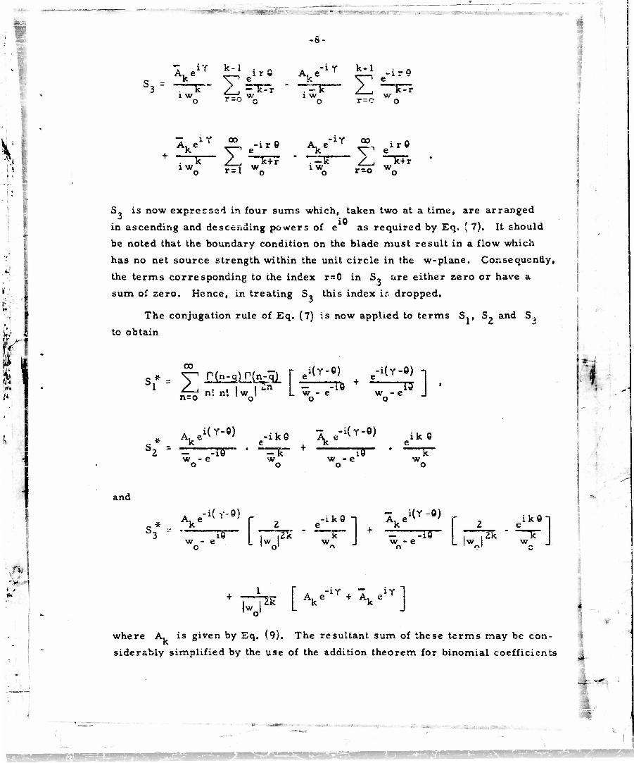
S- is now expressed in four sums which, taken two at a time, are arranged i6 in ascending and descending powers of e as required by Eq, ( 7). It should

be noted that the boundary condition on the blade must result in a flow which

has no net source strength within the unit circle in the w-plane. Consequently,

the terms corresponding to the index r=0 in S., are either zero or have a

sum of zero. Hence, in treating S, this index ir, dropped.

The conjugation rule of Eq. (7) is now applied to terms S., S, and S,

to obtain

oo

s*= YI&iRlLiz^L 1 ^ ni n! Iw |"n

n=o o

r i(Y-e) ,-i(Y-8) e ' , e = 3Ü + ~ L w - e w - e o o i

Ake'(-.) e-ik0 \e-^Y-8) ik 0 e -id w - e o \v w - e o o

k w o

and

Ake i(r 9)

w - e o iff

-ikO 1

w ,2k w

Ake i(Y-O)

w - e n rr

ikOn

Llwj 2k w

i

•*»

M

w p* [ -IY "" A, e T + A, k k .*]

where A. is given by Eq. (9). The resultant sum of these terms may be con-

siderably simplified by the use of the addition theorem for binomial coefficients

-..~^

'

»•-

... •9-

I

which in the form suitable for use here is

S i

—!— > r(-a) m=o aP(-a) mT

The result of these operations is

M &—L

!

6w

<lr^ n r w pr* " UCOSY O O

ei(Y-0)

= ^5" . w -e c

i(Y-0)-|

»v -c o

N cos Y

10 1 +

w -e o TO

e"i0 1 -—^ w -e J

F2 +

.i(Y-W - -i© w -e e

IT" wQ-e

00 ou r

r (m+n-q) r(m-q) e inO

(m-n)! m! Iw I w - * o o

Vn+n-q.)r(m;q)e I 2m

i nfi

(m+n)! ml |w w

1 t (iOa)

where F., F, are hypergeometric functions defined by

F = F(-q, -q;l;-^--2), F, = lim f F (- q, - q; « ; -*±-y) 1 1 |w r L e ~» 0 L Iw r J

.9

Kf ar.= J V i r? #»•-»»*» W*» ^k* series

oo

F(a,b;c;z)= "('} y n^n)r<bt,) B« ( r(a)r(b) ^ iir(c+n)

(10b)

Unfortunately, there seems to be no way to reduce the double series to a

single series. However, this equation does provide the displacement flow

velocity distribution around the impel"er blades and in any specific case pre-

sumably these terms could be evaluated. Equation (10a) represents only part

of the complete displacement flow, for in order to establish lift or torque, the

Kutta condition must be prescribed at the »xit tip for a pump or at the inlet

edge (w.) for a turbine. Consequently, in determining the head-flow rate

characteristics the values of V- and Vö will be needed, i.e., those

I -

_Mi<-il f". "• • - 'V" • ' . ,

i • velocities corresponding to the exit and inlet blade tips. Fortunately, the

factor of the double series (Eqs.(lO)) vanishes at these points. Let V,

and V, denote the tangential displacement velocities at the exit and inlet

tips. They become

1 I'

•

'd2

and

'dl

to cos "T7;

mcosy

X. w -Is!

TTp l

w -lj o

-- T

w

w

Lw -U o

v ",q r

2F N i + c^V^2-2cOSY)F2J '

(Ha)

-lj Lw -l. N 2F. Ü— (p, + 2 cosy) F, 1 cos y 1 ' ' 2

where

= l-o-1! • |wo-wJi

(lib)

(12)

Equations (11) are Busemann's principle results.

IV. The Through Flow

In this section the flow from a source-vortex through the stationary

(nonrotating) array of blades is worked out. Inasmuch as the through flow for

normal pumping and turbining is slightly different they will be discussed

separately.

a. Pump. The point w represents the origin in the z-plane, and all

of the through flow is supposed to originate there. In the w-plane the solu-

tion of this flow is obtained by imaging a source vortex at w in the unit

circle, This flow potential is

-

•

1

fit • *

G(w) = -TZ loE (w " WJ + TT lo8 ( ~, " WJ (13)

where A - Q + i H , Q and P being the source and vortex strength respec-

tively. In order to see the significance of A let w--*w so that z —+ 0 ,

Then from Eq. (1)

w - w—> const x B o N

. • - - . ,

•—PB—«——IB—IEM— '-^^mmamum^'-'-^^ •~r^r">aummmsa

IjN

7

• W.IIMIXW«^ Jim -•.-

Hence, near the origin in the z-plane

M N (a)-* 4~ log z" = ./-(C -> \P ) (log |z| + i Arg z) ,

and the stream function is

N * = -^r (H log | s| + Q Arg z) .

The angle between a radial line and the tangent to the streamline is given by

0,-yy- tan al = r -^- = - P/Q , (14)

HI ui •>R i

•;.K.

.4/4

where Q is positive as shown in Fig. 3. Hence, it can be seen that the

streamlines issue from the origin on logarithmic spirals inclined at an angle

Q, to any radius.

The velocities on the unit circle may be found by differentiation of Eq.

(13) and they are found to be

1 + i tan a. i

J Vrw-

lVew= £ [(1-itanaj)

w w-w

w (

itanojl *

xrrj ' \i w o' ';

The radial velocity is zero as it should be and upon reference to Fig. lb

it can be seen that for w - 1

Q cos Y IT p.

(tan Y - tan a.) (15a)

i

and similarly,

Q cos Y up 1

(tan Y " tan a,) . (15b)

fir

< / b. Turbine, In the case of a pump the flow issues from the origin and

approaches the blades with a pre whirl characterized by the angle a.. How-

ever, in normal turbine operation the flow progresses radially inwards and

approaches the impeller with a given angle Q? positive in the same sense

as a.. The potential for this flow is obtained by merely replacing Q by

- Q in Eq. (13). Thus,

is-

•«IHK

1 •> _

- • -

4

i

i

i it ' 9 id. D

tan a2 - P/Q

tor a turbine and also

Q cos r ' trp-,

(tan Y - tan aj

Qc°Sr (tan Y- tan a,)

(16)

(17a)

(17b)

for the velocities at the exit and inlet blade Lips.

In the development of the characteristic head equ3t;.on for a turbine we

shall need to use an expression for the circulation which muäi be put around

the blades in order to satisfy the Kutta condition at the inner blade edge

(w = w.). However, this flow differs from that of a pump inasmuch as it must

not disturb the flow conditions at infinity,, Consequently, the potential for this

flow in the w-plane must consist of a vortex at the point w with an image at

the inverse point within the circle. Thus if H is this potential,

H(W) = i 2ir

log (w-w ) i r\

log(v-l/wJ. ;i«)

The velocities at the outer and inner blade tips are then respectively

r. T, =

T IT

I

p. - 2 cos Y

P2

p. + Z cos Y

(19a)

(19b)

where I ' is the strength of this vortex.

V, The Head Flow-Rate Equation

a. Pump. From elementary considerations the head of a pump can be

shown to be

H = U, V - Ü. V 2 u2 1 ui

.'

'

•

13- i

t

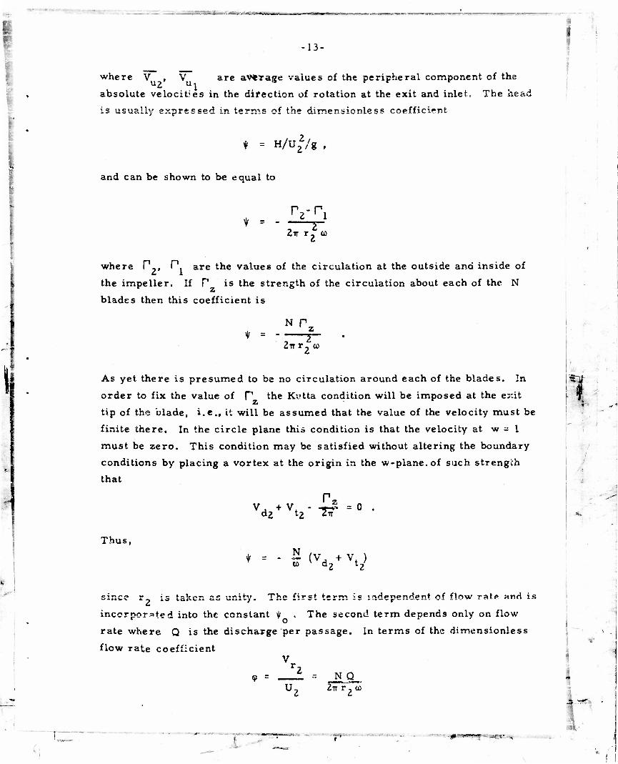
where V , V are aVtrage values of the peripheral component of the

absolute velocities in the direction of rotation at the exit and inlet. The head

is usually expressed in terms of the dimensionless coefficient

* = H/U^/g

and can be shown to be equal to

* • 2TT r- co

? !

J

where P., P. are the values of the circulation at the outside and inside of

the impeller. If p is the st

blades then this coefficient is

the impeller. If p is the strength of the circulation about each of the N

* = N Pz

:—r" ZTT r. co

As yet there is presumed to be no circulation around each of the blades. In

order to fix the value of P the Kvitta condition will be imposed at the eidt

tip of the blade, i.e., it will be assumed that the value of the velocity must be

finite there. In the circle plane this condition is that the velocity at w - 1

must be zero. This condition may be satisfied without altering the boundary

conditions by placing a vortex at the origin in the w-plane.of such strength

that

P, d2 t£ 2IT

Thus,

+ = N to <vd,+ vt>

—' *uwv Lt^ L. CLXX V- * * t*. ta» l* k * * V V The fi^st terrr is m^npn^nf r»f flnw rat.p and is

incorporated into the constant i/ , The second term depends only on flow

rate where Q is the discharge per passage. In terms of the dimensionless

flow rate coefficient

!1 X •

•

•

i •

•4,

<? = u.

N Q 2ir r, ü>

i

T.MV.JJ.». .—^Bm^rzHHpegHmfpr*

-14-

the head equation assumes the form

* + <p Cw (tan Y - tan a, ) o JH

for forward curved blades (Y > 0} and

• = * - <P C„(tan Y- tan cu) O rl x

(20a)

(20b)

for backward curved blades (Y< 0). The shut-off head coefficient ^ is

found from Eq. (11a) to be

4 cos Y

*o = CH [4%-] «P [-****-("*-«>]

• [Fi + N (& -1) F; where

H

_ 2 cos Y 2a sin 6 cot Y CH = " = 5 , " r2 1 + a -2a cos o

(21)

(22)

This coefficient represents the effectiveness of the blades in guiding the flow

whereas ty represents the effectiveness in bringing up the average circum-

ferential velocity to the impeller tip speed. It is evident from Eq. (21) and

Fig. lb that 0 £• C„ ^ 1 . Values of the coefficient C„ are plotted in Ref. 8

and a more detailed plot is given herein in Fig. 5.

For particular values of r./r?, Y and N, a, q, and <r may be

determined either from Eq. (5b) or Fig. 2. The value of the functions F.

and F? may then be found through the use of the series expansion Eq. (10b)

in order to obtain M , Values of this coefficient are also plotted in Ref. 8 o for various values of r, /f ify, N and y« However, these graphs, although

quite useful, are not too accurate and since in the region of major interest

relatively simple expressions may be developed for the shut-off head coef-

ficient, the following paragraphs will be devoted to obtaining more convenient

formulas and charts.

Calculation of values of \Jr0

It is clear from Fig. 2 that if the number o£ blades is small and the

I -m !•%•• *v.- i _„__.• .

I I i i i

•

I i i

•

[ 1 " J*

- i i

•

- 1R. i i

\ radius ratio r\/ry near unity, then the parameter a is large and con-

sequently the expansion of the hypereeometrie functions F,, F, will contain

only a few terms so that '.hese cases may be easily worked out« However, the

majority of cases for pump and turbine applications turn out to be in the range

of the parameter 1 ^ ar/Zn ± 2 . An inspection of Fig. 2 shows that the quan

tity Jw | = a is about unity for these conditions. This situation is for-

tunate because the hypergeometric functions F,, F, permit easy expansions

to be made when the argument is near unity. In particular, the expansion 9

around the point 1 of the hypergeometric function is

^••»•flHS») W^W^/ffi*««* c-a-b

:! •

F(c-a, c-b; 1+c-a-b;1-x)

provided none of a, b, c are negative integers.

Let —» • 1 - A, then the two sums F,, F, become

P(l+q)r(l+q) i.si.A.aüLslika) A2----]

q+q 2(l-q-q)(q+q) J

sm-rr q

IT sin

(23)

ISiSLSl r(l^q)P(Uq? AUqi-q [* j + ܱäHÜ2 A • • - • I (24a) •"(q+q) P(2+q+q) L 2+q+q J

F2 = = r{l+VHL . [lt qq jii- -] «intrgsin^q Pj^jj PJi+jfl Aq+q

Nr(ltq)r(l+q) L 1-q-q J IT sin w (q+q) r(l + q+q)

1 + . ^i^ A + • • • | 1 + q+q J

(24b)

| !

. With the aid of Fig. 2, F, and F, may bi simply romputed for any given

2 case. Again as is evident from Fig. 2, A 3* a - 1 becomes quite small and

nearly independent of Y for about cr/2ir > 1.2. Since Eqs. (24) depend

largely on 1/a , it can be seen that both they and the coefficient y will

t. - • • • »i-«* » t

-16-

rapidly approach the limiting value given by ?. = 1. If then, only iirst order

terms in A are retained

I

= C

, 2 Ysin 2 Y > expv-- n -)

max H

(2 cosy)

4ccs2Y lr(l+q)r(l+q) L NJ

—R

1 T~ 4 cos Y L P(l+q) P(l+ q)

4 cos Y

P(l+q)HH-q) (A) N

P(l+q+q)

and

cH - 1 - 4 cos Y

(25a)

(26)

or more approximately

max

/ 2Ysin 2Y \ expv - —!—JJ—H

1 T~ 4 cos Y ft

(2 COSY)

pq+q+q) P(l+q)P(l+q)

U*P)

The gamma function factor may be directly calculated from its product defi-

nition, however a convenient expansion for it is

JCiita+ai = exp [6. 5797 S2&L - 19. 233 S»i-i- p(i+q)p(i+q) L if if

+ 8.6584 co^T. (8 cos2 r-l)+ ••• N

(27)

4 CO 6 Y Although this series diverges for i > 1 it is rapidly convergent for

values of this parameter less than about a quarter. For Y = *r/2, q is real

and any of the tables of the gamma function may be used. From Eq. (25b)

m

i

' - "^ ' *f?y \

-17-

it can be seen that \|i - 1, and the equality sign only holds for the case of

N = co.

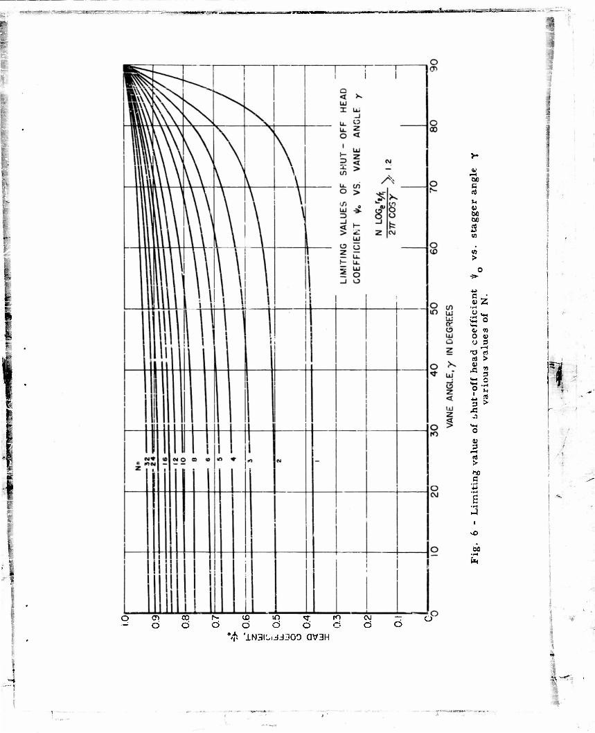
Figure 6 is a plot of the limiting or maximum value of if figured

from Eq. (25b) vs. the blade angle Y for various numbers of blades. If the

geometrical parameter <r/2ir is less than about unity, more accurate values

of the shut-off head coefficient can be computed from Eq. (25a), However

the proportions of most designs are such that Fig. 6 gives a good estimate of

this parameter.

Condition of shockless entry

The head flow-rate characteristic (Eqs. (20)) is a straight line and in

potential flow any point on that line could be achieved in operation. However,

in the flow of a real fluid, large viscous effects may be expected to occur for

highly unfavorable pressure gradients in the inlet portions of the impeller.

For forward curved blades, an infinite velocity always occurs at the blade

inlet edge, however for backward curved blades there is one flow rate for

which finite velocities result at the inlet and this condition is variously known

as "smooth entry" or "shockless entry". For shockless entry, then, the

velocity is finite everywhere on the blade and presumably real fluid effects

should be minimized at or near this operating point, other things being equal.

Hence, the present calculations should be expected to give the best design

predictions at or near smooth entry.

In the w-plane V(0.) = 0 for shockless entry and hence

V + V dl h = 0

is the condition that must be satisfied. The value of the circulation P can z be expressed in terms of the exit velocities so that

*

. ^'

' . ' j

1 •

"-"i '

i

I

(V. - V ) + (V, - V. ) d1 d2' tj t2'

is the requirement. From Eqs. (15)

= 0

V - V *i l2

Qcos Y ,. , v / 1 . 1 v 3 • • - • (tanY- tanoj) (•— + —)

and from Eqs. (11)

»

f 1

iMIMur

-18-

- J9

dl d2 ~ LV1! LW -iJ l - ?! P2

3

Hence,

NQ q — q

(tan Y- tan Q ) = - \ Z°J L^J^-NF L o J Lw -1J

(28a)

As before, most interest is usually in the case of <r/2ir > 1 or a - 1 <* 1 .

In this event Eq. (28) may be evaluated with the use of Eqs. (5c) and (24).

Then,

F NF^_ Nsinirqsimrq P (l+qj Tjl + qj ^2^^

IT sinir (q+q) P(l+q+q) Ha+q+q)

r(l+q)f(l+q)

2 . a -1

&-

or for 4 cos Y/N << 1

2 4 cos Y

ir MT? /, , 8ir cos Y ^ Hl + q) r(l+q),„ 2 . Ä /4ysin?.Y \*l F -NF? = (1 + V ' ) —»—3*—1—a/ (4 cos y) exp( ' <f -Xr-, 1 2 6tf P(l+q+q) N 2

Equation 28 can now be put into the more usable forrr

i o 2 2 r, u ** . \ 1 /i ^ 8^ cos vw 1, <pe(tan Y- tan c^) = - r (1 + 7—j-H (~)

°m ax

(28b)

with an error of less than 2 percent if tr/Zv > 1. 2 or so, since the next term

gives an additional factor of

2 , , 8 cos Y / o- - 4Y sin Y \ 1 + «• exp(- •• v • ' • ) N rN 2 cos Y

i«4 1 «

•

which amounts to about a percent at most for the case considered here.

The significance of Eq. (28a) is brought out by noting that for the simple

infinite var.e theory 2 rl

<? (tan Y-tan a ) = - (—) eoo l r2,

-3 l

X »•-^B,»N«J«J I > I, •

••'. • ir-T

- «atf.umm

-19-

in which the subscript oo denotes an infinite number of blades. Thus we have

<p , ,22 Is. = JL (i + 4" c°s I) (29)

ao %i ax 3 N

Since y £ 1 it is evident that the flow rate for smooth entry always occurs

at a flow rate greater than predicted by the infinite vane theory. This correc-

tion is important siikce from Fie. 6 typical values of i|f may be 0.65 to °max

0. 8. Thus if corrections are not allowed for, errors of 30 percent may be

made.

Figure 7 is a plot of the head characteristic equation (Eq. (20)) for

forward curved and backward curved vanes.

b. Turbine. The same considerations are used in developing the

characteristics for turbines as for a pump. In fact if the flow-rate is suf-

ficiently high for a pump with backward curved blades, a brief inspection of

Fig. 7 will show that the bead is negative and hence power is being tak°n out

of the flow. However, turbines normally operate with the flow directed

radially inwards, and the above situation is termed "reverse turbine" opera-

tion. In the condition of normal operation, then, the flow is inward and hence

the Kutta condition must be applied at the inner blade edges.

The head drop across the impeller will be the same as for a pump,

namely

N r

2* r22 »

'-» 1

•'

The Kutta condition at the inner blade edge (w,) requires that

vt + vd + vr = ° • li di ri

With the aid of Eqs. (lib), (17b) and (19b) one obtains in a manner similar to

that of Eq. (20a)

»|fT - c». CH(ian Y-tan a2) - <|»Q (30)

jp> l«H 11 iin im i «

——m•

5«

where

-20-

'oT cos Y

q — q w I r w -1

o o w -if

o J LW -1 o

N 2Fr^TY-(?i + 2cosY)F2

(31)

The subscript "oT" refers to the turbine "shut-off head".

It is of interest to note that for valuer si y where

<p ^ ^oT^CH ^tan T" tan a2^

the head of the fluid increases in passing through the turbine and thus we bftve

the analog to the reverse turbine, namely, the inward flow pump.

As in the case of the pump, most turbine configurations have values of

the parameter c"/2ir > 1.2 vHch means Lhat a« i and P-.& 0. In this

event f _ can be closely approximated by C X

oT

w q - — I l w_

w -U o

(FrNF2)

This expression is seen t^ be nearly the same as that of Eq. (28a) so that one

has approximately

oT

IT A 2 2 r. H_ (i+in «LJL)(JL) . ~„„ 3N' 2

(32)

max

f

The behavior of the turbine shut-off coefficient is thus similar to that of the

flow-rate for shockless entry of a pamp.

Figure 8 is a plot of the characteristic equation (Eq. (30)) for a turbine

for various values of a?. For normal operation a? < 0 and the sense of

rotation is opposite to that of a pump with backward curved blades. The con-

dition of no leaving whirl usually represents a useful approximation of the

design operating point for most configurations.. This condition is easily ob-

tained from the inlet velocity triangle to be

= - tan Q.

T W'^1

n- -21-

fe!

Shockless entry

Reaction turbines, in general, have blade shapes which differ substan-

tially from that of a logarithmic spiral so that smooth entry calculations based

on the present theory are not too meaningful except possibly for a pump of con-

ventional design run as a normal turbine. In this case, the calculation pro-

ceeds in the same manner as that leading to Eq. (28a), i.e., the condition

V(Ö = 0) = 0 must be satisfied. When this occurs, the velocity at both the outer

and inner blade edges is finite and it is clear that this condition corresponds

exactly to that of a pump operating at shoekless entry except that the direction

of flow and rotation are reversed. Since the Kutta condition is satisfied at

both points, the flow is reversible and the shockless entry computations for a

pump can be applied to turbine operation.

Torque characteristics

Turbine performance is not usually presented in terms of the dimension-

less head and flow coefficients y and f unless the speed is maintained

constant. If the speed is not constant, torque is given as a function of angular

speed with either the head or flow-rate kept constant. In the present work it

is most convenient to hold the discharge constant. The torque can then be

expressed by means of the dimensionless coefficient X

*= PA2Qr2Vr2 = ^ (33)

where here p signifies density. In the case of a real fluid the efficiency is

given by

^T ~

This torque coefficient is to be distinguished from that of a pump operated at

constant speed which is given by

and where the efficiency is given

:

-

!

i 4 '

22-

The torque coefficient can be expressed as

K - C„ (tan r - tan a,) ft ' c Vr (34)

with the use of Eq. (30). Thus "X is a straight line function of l/'{>. The

intercept of — » 0 represents the locked rotor torque, and the value of l/m <P

for "X = 0 represents the turbine runaway speed. These results are shown

in Fig. 9.

•

VI. Extension to Nonlogarithmic Spiral Shapes

The theory as presented thus far is limited to flow in strictly two-

dimensional radial turbomachines. The simplified shapes demanded by this

theory are seldom realized in actual designs. There is no doubt that the

effects of blade angle and passage breadth variations, in addition to meridional

curvature can cause important deviations from the two-dimensional theory.

The flow through an arbitrary cascade of airfoils is a related but simpler

problem and it has received great attention in the past twenty years. Un-

fortunately, it is quite difficult to get an exact analytic solution even for a

circular arc profile although special cases may be worked out by Garrick's

procedure. Thi'- difficulty was partially circumvented by employine approxir 13

mate methods similar to that of the thin airfoil theory. The work of Rannie

is among the most useful of these except that it is restricted to circular arc . 14

camber lines. Integrals for other shapes have been given by Pistolesi

but not evaluated.

There seems to have been relatively little analytical work done for an

arbitrary radial array of pump blades. Calculation schemes using Ackeret1 s

method of the continuous distribution of singularities have been worked out

for pumping configurations by Betz and Flügge-Lotz, but this method does

not permit general analytic solutions to be obtained.

In the sections that fellow a theory for nonlogarithmic spiral blades will

be outlined. Like the work of Rannie and Pistolesi it is based on the ideas of

thin airfoil theory. As the smarting point for this method the solution of a

more general boundary condition than Eq. (6) will be obtained. These new

I

-

s • 7—^rt "*"r .

•

-23-

solutions r.ri then interpreted from the point of view of perturbations on a

logarithmic spiral and correction terms for the head and flow-rate equation

are obtained. The resulting blade shapes can be quiie general and no restric-

tion to any particular variation i* necessary. These solutions ?re also em^

bodied in further approximations to account for the non-uniform breadth of

most impellers. Finally, a simple correction for nonradial, i.e., conical

flows is given.

a. Solution for any Power Boundary Condition

Suppose that on the surface of the blade (Section II) the normal velocity

is to be

m+1 |V = ku cosY r n (35)

where r, cc, f have the same meaning as before and k, m are real constants.

The vector velocity is then

V =k co cosy zx |zjm .*<»/*+ Y)f nz b • b'

and following the procedure leading to Eq. (6b) the radial velocity in the w-

plane becomes

kcocosY ."•"TT— - i im fei(Y-9) e-i(Y-e) 1

rw zb % l2bl — -iö w -e o id w -e o

Now

zbZb lZbl m m+2

i

<•

A

t

\

and since |z,| is given by Eq. (6c), j zv

2 by m+2 to get

may be found by replacing

-b m+2

w -e o w -1

m+2 — iO ' "2- q

m+2

w -e o •iO

Thus the radial velocity in the circle plane can be written as

k CÜCOSY

V *-i N

r w

iG w -e o w -1

o

rei(Y-0) e-i(Y-S)

- -iö." " TT w -1 w -e w -e o J u o o

w -e o

(36)

r •

—I .— . - "-? Ifc» llliuaa. i..i.u .«•„•»<%* --

24-

<

,fft

• •

I

•here 1 2iY

or 2 N m + 2 N

(37a)

(37b)

The geometrical constants of the mapping are still determined by N, r\/r ?

and Y • Equation.(36) is now formally the same as (6b) except that q

has been replaced by., q'. The tangential velocity corresponding to boundary

condition Eq. (36) is ifte same as Eq. (11) except that q and quantities de-

rived from it are replaced by q'. Thus

...' kwccsv o o 2 N p- w -1 ! — , 2 L ° J L^v1

W_ 1 «' (- W i 1' r 2FS + N'

1 cos Y (p2-2cos Y)F2 , (38a)

and

' kcocosy Vl = " N pj

where now

w o

w -1 I O

o

Lw -1 J o [ 2F, +

N' I" cosY

(pl + 2COSY)F2 (38b)

'. = F(-q-, -q«;

l%l Equations (38) are the exact solution of the potential boundary value

problem given by Eq. (35).

b. Application to the Through Flow

Before the typesof approximations to be made are discussed it is illus-

trative to show the applicability of Eqs. (38) by using them to obtain the

solution for the through flow of an impeller with logarithmic spiral blades.

If in the z-piane there is a source flow issuing from the origin at an

angle a, to the radius» the velocity along a streamline can be shown to be 1

NQ 2IT r

1 COS CL.

',-_•- \

- ._ - * * -T

1

—:

This velocity has a component -V normal to the blade, and in order to make

the blade a streamline, a flow must be added which has a component V^ that

will cancel the contribution from the source. If Y is tne angle of the blade

to a radius then this component is

V = N Q sintr-aj) n 2 IT r cos a,

By inspection of Eq. 35 it is seen that m = -2 and that

k = NQ sin(Y-0l)

2 IT to cos Y cos a.

Upon substitution of these values into Eq. (38) one obtains

V = - Q C — ' l)

2 2TT H cos ycosa,

which is the same as that given by Eq. (15a) (except in slightly different form)

for the tangential velocity at the point w = 1.

Boundary condition for nonlogarithmic spiral

Let us first consider a log-spiral blade of constant angle Y • ^ there

is a source flow at the origin in the physical plane given by the potential

NQ ,. . , s . -jr^— (1-i tanaj) log z ,

then the velocity component parallel to the blade is

V = NQ 2TT r

COS ( Y - O.)

cos a, (39)

I i

ts->

This flow component is everywhere parallel to the blade surfaces, and the

required solution is given correctly by Eqs. (15). Suppose, however, the

blade angle is locally slightly different from Y (Fig. 10). The condition of

no flow through the surface is then that

V tan« (40)

•

•:

1^ I

-26-

where V is the perturbation velocity normal to the skeleton l:a«; A angle y ,

V is given by the above and t is the angular difference

« = y - (41)

Y being the angle of the perturbed blade. It will now be assumed as is

customary in thin airfoil theory, that boundary condition Eq. (40) may be

applied on the logarithrric spiral. For simplicity it will also be assumed

that € « 1 so that tan e = c . With these assumptions the boundary condition

on the logarithmic spiral may be expressed as

v' = SL2_ n 2irr

cos( Y-Q,)

cos o (42)

If the angular perturbation e is expressed as a power series in the

radius the required solution can be readily obtained by means of Eqs. (38).

The present interest in this work is for pumping configurations and the

function « (r ) will accordingly be specialized to suit this end. For this pur-

pose it is convenient to express e in terms of the circumferential variation

y (Fig. 10). From the figure»

and

Thus

Now if

0" = 0 - y/r ,

tan y = r -r—

tan Y = tan Y J 1 - cot y-£ + X. cot Y 1

i s~Tt

C « 1

then

tan Y = tan y+ «/cos Y

c = cos 2v Lf-Sj (43)

The variation y is useful in laying out impeller blade designs. The

true length of the blade is customarily developed by graphical procedures,

and typical blade variations are shown in Fig. 11 where it is seen that most

' =— r «MW»W>: fi ',- 9 -• > ;~^*^*-

-27-

of the departure from a logarithmic-spiral occurs in the inlet regions. This

fact is also important because it means that the blade shape perturbations

are mainly subjected to the oncoming inlet flew. Hence for this reason the

perturbation boundary conditions are based upon the component of the inlet

flow parallel to the angle Y . This situation is different from cascade theory

in which the vector mean of the inlet and outlet velocities is used.

Perturbations representative of pump design are

and

y = X(l-r)-

fc.-SX(l-r)J

(44)

so that according to Eq. 43

« : • i

•

e = X. cos Y (— " 3r + 2r ) (45)

The coefficient X is determined by specifying « at the inlet (since « = 0

at r = 1).

The equation for the boundary condition now reads

. NQ cos( Y-o ) » T 1 1 V = -EH —i i X COSY -T - 3 + 2r

n 2TT COS O. ! r (46)

The constants k and m in Eq. (35) can now be identified for the three terms

of Eq. (46) ! *

*

NQ cos(Y-a.) , k = (SSL) — i- xcesy; m = -3; N = irr«' cos a. 2N

/NQ cos(Y-a) , k, = - 3 (-—=-) -~- i- XcosY; m=-l; N =2N 2 V2TT«ü ' cos a.

K - * ttt NQ, cos(Y-ttj)

2TT Cü cos a, X. cos Y ; m = 0; N = N

(47)

With the aid of Eq. (38), each of the contributions of Eq. (47) to the tangential

28-

velocity V. may be determined. They are:

a

i

V = -\Z _J L cos^Y-i I(-2N) 't ir cos a.

T\1 Fj(-2N) -J- 2N F2( -2N) 2:N F2( -2N) ^ 2'cosy

- 3J(2N) F(2N)-2NF(2N) 1 -i 1 + , *N. F7(2N)

p, 2 cos Y 2X j

-

+ 2J(N) F(N)-NF,(N) N 1j -i + rr-T- F,(N) \

P2 2 cos x 2* ' j (48a)

and

V, =\H L cos Y { J(-2N) t TT cos a. '

F(-2N)+2NF2f-2N> + „££L-_-F,(-2N)

3J(2N)

+ 2J(N)

Fl(2M)-2NF2(2N) 2N

2 cos Y 2

1

F,(2N)

2 cos Y 2*

^(Nj-NF^N)

TTZTr F2^ 1 (48b)

in which the special notation

J(N) w

w

• -,q w i x r w

o * J Lw -1

has been introduced. These equation» may be evaluated by means of Eqs.

(24) and in the case ef tr/Z-n > i. 2 further simplification can be made.

The through flow solution then consists of the above correction terms

plus the main contribution from the log-spiral solution. In like manner,

correction terms for the displacement flow will be obtained.

c. Application to the Displacement Flow

The boundary condition on the perturbed blade is

-i

, '

••..••

t. . • •*.:. »-ex; I ,

m r

mmimii -7—

29

V = r Cö cos Y = r co cos (y +c ) •

i 7

The parameter c is again supposed to be small compared to unity, and as in

the preceding section this boundary condition is applied on the logarithmic

spiral of Y = const. With these assumptions

V = r © cos Y - « r a sin y n •

is the condition to be satisfied on the blade surface. However, the first term

consists of the displacement flow already solved, the second term thus

corresponds to the perturbation which accounts for the non-uniform angle,

hence i

r to c sin y (49)

is the additional term which must be determined. If the specialized shape for

pump blading is used (£q.(44)) one obtains finally:

V = - X « sin y cos y jl - 3 r + 2 r i (50)

1

The constants k and N are

k. = - X sinycos y ; m = - !, N = 2N

t 2N k_ = 3 X sin y cos y ; m = 1, N = -*-

' N k- = - 2 X siny cos Y i m = 2, N = y-

(51)

The additional tangential velocity contributions are again found by use of

Eo«s (38) to be

i —i • «g_ E,(2N/3)j mm

V,.= -2 col

+ 3K^)

2J(£) F^N/2) - N/2 F2(N/2) N/-->

2 cos Y F, (N/2) (52a)

' , '

:

*£&

T^ZZ '

^-umm^jcr^- '

-30-

und

di 2 cos \ sin YCOS Y "-"H—' , -J(2N)

L

FL(2N)-2NF2(2N) 2N

5 -=- F7(2N) 2 cosy 2

2N r F1(2N/3) - 2N/3 F,(2N/3) 2N/3 E,(ZN/3) + 3J(-5-) |^ 2 v.c Y

N r Fj(N/2) - N/2 F2(N/2) N/2 F?(N/2) 2J(T>4 FT 6 cos Y

(52b)

i

The effect of these perturbations on the head flow-rate equation will

now be considered.

d. Head Flow-Rate Equation

From Section III the dimensionless head coefficient is seen to be

<

* = - H (v + v. + v,' + V.') f tt V d2 h d2 fc2

where the primed quantities refer to the correction terms given by Eqs.

(48) and (52). In ordar to evaluate these expressions the condition <r/2ir> 1. 2

will be imposed. Then if

+ = 2 COSY J(N) F(N)-NFJN) -i £— + —El E,(N)

p7 cos Y 2* ' } to(-2N)Ä l/*o(2N) .

With these simDlifications the head eauation becomes

| = t + •' +jl CH(tanY - tana.) 1 + X cot( Y - a.) cos Y

[rrzHj ,,^1 I

• o^ ' •ox J '

where 1

• ^ = X sin Y COSY [3 *o(^) . +o(2N) - 2 ^(^ ] . (54)

:

••

-

*

• s '* —*.. — *r

*M*:£KAi^

-M

\

Equations (53) and (54) represent approximations which can be made

if the solidity is sufficiently high. For the terms IJL(2N) the approximations

are satisfactory but are less accurate for i|r(N/2). Although more accurate

formulas may be obtained with the use of Eqs. (24)t the present results pro-

vide <t fir »L-or der correction to the head flow-rate equation.

These corrections are applicable for pumping configurations in which

the major blade shape variations occur in the inirt portions of the impeller.

It has already been stated that the shut-off coefficient {, and the guiding

parameter Cu are very insensitive functions of the solidity if it exceeds n unity. Consequently, as a result of inlet perturbations one should expect

only negligible changes in performance. Such indeed is the case in Eq. (54)

since the y terms are all of the same order of magnitude and hence almost

cancel each ether. Thus changes in inlet angle should not result in signifi-

cant performance changes. However, there should be a change in the shock-

less entry condition at least of the same order of magnitude as the variation

of the inlet angle itself.

e. Shockless Entry

The additional contributions of Eqs. (48) and (52) are used in the same

way as the development leading to Eq. (28a). Thus the condition for shock-

less entry is

= 0 . (V. - V. ) + (V, - V, ) + (V. - V. ) + (V. - V. ) = H *2 dl d2 ll *2 dl d2

If the same approximations are to be made herein as in Eq. (54), then one

may use the result

J(pN)[rl(pN).pNr2(pN,] . [1+ü!«|!x.]_^ [li] 2/t

I "

i -

f -

&• The shockless entry condition then takes the form

i

*e 1+B 1+A (55a)

where

1 •**•***......*.,.>. .„a..-/. • dT

•

t" + •-» •».. «"1**-. -k .»

rjr-

Si*>~f' . *m*&~ . .jwr^-'iiriwMBMMjiMa»

3?.-

KJI^. J.H v*".|«

- !

A -- >. cot( Y- a,) cos Y *o<2N> XJ2N) S(*\/->2) 2('x/r2)4

MN)

•'\ ••

I 1 + 8,T2COS2Y 1 L 6N" J

B = KCOSY sinY • (N)

1 + 7*1—T" 8tr cos Y

6N2

3<rl/r2> f_3.2cos2Yl (r2/rl)

*0(2N/3) 1 +

N J

(55b)

i

*A'V •

m • WS*

V*

% •**

2(*,1/'2J"

*0|N/2) 1 + lbir cos Y

3S* J (55c)

The ratio 9_/<Pfc is the ratio of flow rates for shockless entry with and with-

out the inlet angle perturbation. A close inspection of Eqs. (55b, c) shows

that

lij<9 < 1 for \ > 0

*e/*e > l £or K < ° *

This behavior is to be expected since if X. > 0, Y > Y and a "flatter" blade

inlet angle results. This can be easily seen if the limiting case N—» co is

considered, since then

A -» \cot( Y- a.jcos'Y ft- •% ••»)']• B —* \cos Ysir.Y 3

2-1

w-^-ra J Presumably,

A, B C< \ so that

Ü* t 1

I

'

- .1*8-* .

i" i

•1:

(•*•

-a-

With this simplification

- 'i

it

:* A

tanY - tana 1 2 ,° » taniY + e ) - tana

cos Y(tany- tana.) Vl '

which is the simple infinite vane theory. Equations (55) give the correct

limiting value for shockless entry, but this result may be used as a "rule of

thumb" for determining the flow rate for this condition. More exact values

for a finite number of blades can, of course, be computed.

- ' *, -

'•*'• 3ii

'. rK

flth

VII. Extension to Nonradial Profiles

Of particular interest to the designer, is the so-called "mixed-flow"

impeller in which the flow approaches axially and progresses through the

impeller on more or less conical surfaces. In certain cases it is possible

to apply the results of the foregoing calculations to such impeller geometries

and thereby obtain information in this important field of application.

The principal difficulty in such mixed flows is that the stream function

and velocity potential both do not satisfy Laplace's equation, so that the

methods of complex variables cannot be used. This circumstance is shown

below in Eqs. (56) which are the equations to be satisfied by the velocity

potential & and stream function T for incompressible, perfect fluid flow

over a conical surface with varying breadth b and constant vortex angle X>

l. e.,

1 3 If "SIT

1 3

Rb 3$

R 31 F^oTf R"

-JBL- 3-£^

3J>

i 3 = o

(56)

The coordinate system is shown in Fig. 12. In the derivation of these equa.

tions it has been assumed that the curvature of the waU is small so that

variations across the passage breadth may be neglected.

!

-

\

\

k

i....

-34-

T.t is clear from Eq. (56) that if the breadth b is not constant then

y and Y both do not satisfy Laplace's equation. However,, an important

deduction concerning the special case b = constant caii be made.

a. Flow over a Con\c*l Surface of Small Constant Breadth

If b is constant and if there are no variations across the breadth then

Eqs. (56) reduce to Laplace's equation in the conical coordinates R,i>-, and

the two-dimensional calculations may be applied as follows: First, it is

clear that if there are N blades, that the flow on the conical surface is

periodic with a period of 2ir sin £/N. Thus if there are N blades on the

cone, they are equivalent to N/sin X, in a straight radial array, i.e.

N* = N/sin K . (57a)

The other geometric properties of the array follow in a similar fashion. The

radius ratio R-/R. = r?/r. remains unchanged. The solidity parameter

becomes

_£ _ NlogrZ/ri 2TT 2TT sin £ cos y (57b)

The boundary conditions for the displacement and through flows are also the

same as for the pure radial flow. This result is easily shown, for on the

conical surface

V = SxR COSY =Rö sin X. cos Y = r « cos Y . n

Hence, the radial flow calculations may be applied to the flow in a conicai

impeller of constant breadth if the equivalent number of radial blades is given

by Eq. (5 7a) and the solidity by Eq. (57b).

An interesting limiting case is provided by making K—» 0 but keeping

er constant.

it R--R. is the slant blade height then

cr 7Z

Nlcg(H- -^~) Ztr sin £ cos y

and as C —? 0 and R? sin £ = r? is a constant, one obtains

•*

•

? *<VR1> ?TT T- COS Y

which is the definition of solidity for a two-dimensional cascade. The flow

coefficients of the radial case also become equal to the cascade results since

if <r is constant and N/sin K —> oo then the head coefficient (Eq. (25a))

become s

*osCH

which is the cascade result.

b. Effect of Variation in Breadth

From the foregoing discussion it is evident that a realistic treatment

of the effect of breadth variation cannot be done by complex variable methods.

However, if db/dR is small compared to unity then approximations based on

complex variable methods should give correction terms of the right magnitude

and in the limiting case of an infinite number of vanes, converge to the exact

answer.

For the sake of simplicity., in this section it will be assumed that

K =90 , i.e. , a straight radial impeller. In Section V-b, the through flow

solution was obtained by computing the "interference" velocity necessary to

make the blade a streamline, and using this velocity component as a boundary

condition in Eqs. (-6). Nov.' it is clear that if the breadth is varied, the

interference velocity will be changed and hence a different flow will result.

In this section the j-.d6iticr.al terms for the through flow wilt be worked out.

Inasmuch as the disp1^cement flow boundary condition is independent of the

breadth, no additional correction terms should be expected to occur,

11 :

»

r. The boundary condition

. V •- ££ n 2irr

sin( v - a\) b^ cos ai b[7) (57) '

> •

vmm* a—i

-36-

•

I 1

applied along the blade surface makes it a streamline in the through flow

where h> and b(r} are the impeller widths at the exit and at any radius

respectively, and y is the angle of the perturbed blade as before. The re-

striction t =Y'~Y < < 1 will fee retained so that

sin( Y - a.) = sin( Y -a,)+ « cos(Y-a,) ,

and if the breadth term be written as

b2/b(r) = 1 + f(r)

the boundary condition becomes:

NQsin(Y-o,) NQsin(Y-eu) V = , l

n 2ir r cos a. '1 "27 r cos a,

(58)

NQcos( Y-a,) ,- -j f(r) + < —_ L l + £(r) >- r cos a. L 1 2ir

The first and third term of this expression have already been worked out in

Sections III and V-b respectively. Thus the additional term required for

breadth variation is

\T n

NQ sin( Y-a,) r -i -i- f(r) [1 + c cottr-ajjj . T7 r cos a (59a)

1

In keeping with the spirit of the foregoing approximations, e will be neglected

compared to unity. It should be pointed out that this assumption results in a

linear theory. In order to obtain the solution of Eq. (59) by means of Eq. (38)

the function f(r) must be expressed in a power series. Although any parti-

cular function could be worked out, it seems most to the point to evaluate the

effeci. of breadth variation for the simplest case possible, namely, a linear

one. For some mixed flow designs this is a fairly realistic choice but

Francis type impellers require more complicated functions. Thus, assume

%

1 . '

•

so that

\r _ v — n

i{r) = u(l - r) ,

NQsin( Y - a.) , „ -, -L (i. - i) '» cos a, r ' -2T

(60)

(59b) 1

•

\ •

•^rfrstmmsausm^rr^s^t

-37-

In terms of £q. (35) one has

NQsin( Y- Cj) , - u. • .. • i ; m=-2, N =00 1 r 2TT (ocos a. cos y

NQsin(Y-aj) 1 k, = - u .a. .,, ., 1 ., . - ; rn - - 1, N = 2N

2 • 2TTCO COS a. cos y

hence the perturbation tangential velocities (found from Eq. (35)) are

Q sin( Y-oJ

and

ir

•n cos a i

J(2N) f F1(2N)-2NF2(2N) 2N

( 2 cos Y 2 F(2N) \ - -L

Qsin( y-Qj)

t 1

TT cos a 1

f F,(2N)-2NF,(2N) 2N 1 . J(2N) * -i « 5 *N

V F,(2N) - ~ 1 Pj 2 cosy 2> 'J p

(61)

These results may be used in conjunction with Eqs. (48) and (52) to obtain

correction terms to the head flow-rate equation. However, one may expect these

terms tobe small for pumping configurations and also that the only major

change will be in the condition for smooth entry.

With the former restrictions on the solidity one has approximately

11 11 Q sin( Y- a.) Vt "Vt s* IT COS ä

1 *o rzNj -L+JL pi n J

When this expression is included in the shockless entry condition Eq. (55a) 1

remains unchanged except that A is replaced by A , i. e. ,

i 1

or 11

Is. 9.1

1 4 B 1 ? A' '

1 + A

(oua)

1 + A' (60b)

1

••-• -'.Mi";

-38-

where

A - A + L r2 ijm -1 (61)

and » is the flow rate coefficient for shockless entry for an impeller with

variable breadth and nonconstant blade angle. The coefficient A is given by

Eq, (55b).

If \i > 0, th& impeller inlet is smaller than the exit (Eq. (60)), »o that

the shockless flow rate must decrease (Eq. (60b)), However, the usual case

is that the iniet breadth is greater than that of the exit so that (j. < 0 and the

ratio

> 1

In the limit N -+ co, Eq. (60b) becomes

<P b, re 2 to DT Ye 1

(62)

which is precisely the result of the infinite vane theory. If there is no pre-

whirl (a,= 0) this limiting condition can also be written as

tan Yj b2 tan Y2

= *7

where now y is the relative flow angle at the inlet for two different breadths.

Both this equation and Eq. (62) are really the conditions for maintaining the

same incidence angle to the blade inlet. Without undertaking detailed calcula-

tions this result is probably as good a rule as any other for inlet breadth

variation.

More complicated breadth variations could be used to account for dif-

ferent profile shapes. However, it is doubtful whether or not they will add

significantly to the results of Eq. (60) in view of the already approximate

nature of the solution. In fact because of the obvious crudeness of the breadth

approximation* we have oeen somewhat hesitant to present them, and have

done so only because we are unable to find similar computations elsewhere.

.

,- J

i

* : 4 '

_v„^*_^

-39

c. Remark on Application to Mixed Flow Impellers

With the aid of the theory developed thus far it is possible to make more

extended analytic computations of mixed flow impeller performance than here-

tofore possible. Thus far, the effect of the blade forces on the meridional

streamline distribution have been neglected. Tn the case of radial or mixed

flow pumps the deviations can probably be overlooked at least at the design

point unless blades of unusually high "warp" are employed or if the total

head distribution is not uniform across the passage at the design point. In

any case, these effects may be approximately calculated by theories recently id 17 made available. '

For most conventional designs with constant total head developed across

the passage it will still be necessary to obtain ike meridional streamline and

velocity distribution and thus work out a "pseudo-three-dimensional" solution

by application of the foregoing theory to each stream lamina. The blade sec-

tions can then be designed to have smooth entry occur simultaneously across

the inlet or any other condition.

This discussion: will be closed by observing that although the present

theory is applicable for the straight radial or conical profiles it is still

inadequate for the smooth entry calculations of Francis type impellers with

rather large meridion curvatures. In this situation the flow may be imagiaed

to take place on an infinitesimally thin lamina of revolution and the methods IS of conformal mapping can be applied to this "two-dimensional" problem.

d. Remark on the Influence of Compressibility

A general treatment of the radial flow turbomachine problem is too

difficult to be attempted directly. Specific cases have been worked out numeri-

cally for the pressure and velocity distributions in the passage. Radial flow

compressor configurations in general have rather high values of the solidity,

e.g., c/Zir ^ Z are not uncommon. For these cases it seems reasonable to

suppose Lixdl the design Coefficients i and C H

are still quite subsonic. That this is indeed the case is shown in Ref, 1

wherein the value of the coefficient ^ differs by less than one percent for

an impeller operating with a tip Mach number o£ I, 5 and zero. In fact, the

value of these coefficients for compressible flow is'Only about one percent

• f S ' —TZ. ~USr -,

- '^Rö0^•^w'', *—ojSrr--~**'t

-40-

different from the results given in Fig. 6.

Thus, it would appear that for configurations of high solidity the in-

compressible calculations give a good approximation for compressible flow

performance, except for the maximum mass flow which depends mainly upon

the inlet design. The head flow-rate curve should then be nearly the same if

the volume flow parameter is based on the exit volume, i.e.,

u. m

where m is the mass flow-rate/exit area/sec and p, is the exit density.

The total pressure ratio then becomes

i

Pi

U2 C„m(tanY - tana.)

p ^ po(p7J *2

+ 1 •

k

(63)

where k is the ratio of specific heats, J the mechanical heat equivalent,

p , T are the inlet density and static temperature respectively.

e. Numerical Examples

In this section a few examples illustrating the use of the graphs will be

worked cut,

1. Consider a radial flow pump of constant breadti. with 6 blades of

constant, angle y = 70 » radius ratio 0.5, and with no pre-whirl, i.e.,

a, = 0. The solidity is

-2- = 6 In l/lv cos v = 1.94

so that icqs. (25b) and (29) may be used safely. The shut-off coefficient i.<

(Fig. 6) t = °«81 and CH = l*00' Thus the head flow-rate relation

(Eq, (2 Ob)) for backward curved blades becomes

f = 0.81 -2.745 0 ,

th« condition for shockless entry is (Eq. (29))

, '

-;

—*—'•*.%;.. j-. .— I. >..

-4 ) - !

8TT2COS270° 6 - (\ , OTT COS iU x _ , ?Q

eCX3

or 29% more than the simple theory would indicate. Now

thus

<p = (*,/*,) cot y = 0.091 eoo * £

<p = 0. 117 e

•

Since there is no inlet whirl, the absolute exit flow angle a, is given by

tan a, = ff/q 2 " T/*

or

= 76"*

at the shockless flow rate.

It should be emphasized that ty is only a parameter useful in deter-

mining that part of the head curve near tne design point. Cress *eal fluid

effects prevent \|i from being realized near shut-off. »

2. If it is desired to operate the pump of Ex. 1 at a shockles« flow rate

of $ = 0. 100, then the inlet angle y. will have to be increased (i.e. made

flatter). Thus from Eq. (55a)

^e 0.100 tfT 0. i i 7 f = 0. 85S

'

Since y , N, r./r^ are known, X. in Eqs. (55b, c) can be found. For a. = 0

hence

A = 0.0324 X

B = -0.224 X

X = 0.566 .

* • .-tj; »

,

By Eq= (45)

-42-

t = 0.0664 = 3.8

or Yj-73.8 . The inlet angle must be increased by about 4 in order to

have smooth entry occur at 0 = 0. 100. At this operating condition the inci-

dence angles to the blade is 5. 5 whereas in the case of Ex. 1 it is 5 at

shockless. For this casa then, the simp?" rule of maintainirg s constant

angle of attack or incidence to the blade will satisfy the smooth entry con-

dition. For smaller values of \/2TT, however, deviations from this ruie must

be expected to occur. Without further calculation we may also suppose th-.t

the same result holds true for minor breadth variations.

3. Let the pump of Ex. 1 be operated now as a normal turbine. In

general there will be some whirl leaving the impeller so that a. / 0. For the

normal direction of operation Eqs. (30) and (32) give

ilr= <p(2. 75 - tano,) - 0. 322 .

Typical values of a, are in the interval -80 £S a7 £ - 60 . If the value of o

a2 is chosen is that for the normal pump operation in Ex. 7, i.e.» a, = - 78. 5

then

t s 6. 91* -0. 32

is the performance of the pump in Ex. 1 operated as a turbine. The condition

of no exit whirl is the same as that of the shockless flow rate in Ex. 1, viz.

9 = 0. 117.

4. In the last example a 70 angle pump with 5 blades, constructed on a

45 cone with a radius ratio of 0. 7 will be considered. The solidity of this

configuration is

~7Z N In r2/

ri 2TT sin£ cos

in 2

In sin 45 cos 70 1. 17

which is large enough for ihe approximations of Eq. (25b) and (29) to be used.

The equivalent number of radial blades is N = N/sin X, = 7. 1, hence from

Figs. 5 and 6

CH - 0.983

• • =0.83

o

-du -

" AW1!**IJI""*Vi*! " ... .... ^ '">-.- ' N

•43-

The coefficients y given in Fig. 6 are the maximum values for the given

number of blades. Unless C.. falls several percent less than unity closer ri

approximations of -if do not have to be made. In that event, however,

Eq. (25a) will provide a first order correction.

For a. = 0, ihe head equation is

* = 0.B3 - 2. 70 <p ,

and shockless entry occuvs at

« = <p 1 ;oo Tory

2 2,n< ir cos 70 7TT~

» =0. 222 . *e

If the breadth of the impeller is comparable to the radius then the

analysis will have to be done for a number of streamlines. It is customary

to design pumps in such a way so as to have a constant head developed across

the exit breadth. The meridian velocity distribution is then only slightly

affected by the blade loading and one may use any means to obtain the meridian

flow. However, at "off design" flows, the effect of the blade loading will

become important for small values of K , i.e.? shallow conical pumps, and

recalculation of the meridian velocity profiles by the methods of Ref. 16 may

become necessary.

VIII. Concluding, Remarks

There have been three purposes in presenting this material. The first

ha.s been to outline an f«?rf theorv for "^ocential flow in impellers with loga-

rithmic spiral vanes. The second has been to describe an analytic "thin

airfoil" theory which could account for the effect of blade angle variation.

This approximate theory starts from the solution of the potential flow through

a radial array of log-spiral blades with the normal velocity component being

prescribed as any power function of the radius. A method is shown whereby

these aolutior»;; may be used to obtain correction terms for small variation.?

i

I I

.44,

in vant- angle and cassace breadth and also when the meridional streamlines

are cones.

The last objective has been to develop the theory in a form suitable for

radial flew pump and turbine configurations. Formulas and charts, useful

for rapid performance estimates, are provided for this field subject to the

restriction that the solidity be greater than about 1.2. However, general re-

sults are also given so that other designs may be determined.

It would have been desirable to include a number of detailed impeller computations in which account is taken of the meridional streamline distribu-

tion. Th? work involved is considerable, however, and for that reason such

results are not presented here.

It would also be of interest to extend the present theory to account for

the effect of strong meridional curvature (i.e. Francis type impellers). This

would complete the theory of the "pse-ido-three-dimensional" impeller with

a finite number of blades. The write-« is interested in this problem and would

like to see examples of such calculations made available so that the im-

portance of these parameters could be determined.

1

i

i 1

-

•

H

-45-

IX. Notation

List of Symbols

- Area

- Complex velocity potential, hyper geometric function as noted

- Number of impeller blades

- Flow rate through one impeller passage

- Torque

- Circumferential velocity = rco

- Absolute velocity

- Relative velocity

- Flow-rate correction factor

- Breadth of impeller passage

- Gravitational constant

A

F

N

Q

T

U

V

W

C

a

b

8 k, m, n- Constants

r - Radius in physical plane

q - Complex constant

w • Complex coordinate in circle plane

w - A constant in the w-plane representing the origin of the z-plane • ae

z - Comdex coordinate in physical plane = x + ig

r

X.

\

n

1

<P

- Angle between absolute flow and radius vector, ^ Positive increasing counter-clockwise)

- Angle between blade tangent and radius vector

- Argument of w^

- Angular perturbation of blade

- Cone ancle

- Angular coordinates

- Constant

- Radiu? vector in w-Dlane

- Solidity = Vlnr2/ri

cos Y

- Torque coefficient at constant speed

- Velocity potential

- Flow-rate coefficient = NO./2tr A-,V, -

M-Y

r2 2

r 1

Torque coefficient at constant flow-rate - i»/^

-46-

Notation (continued)

CO

Stream function

Head coefficient = H/U2 /g

Angular speed

Superscripts

- Conjugate i.e., 2 = x-f iy, z = x-iy

- Conjugate function

b

d

c

n

r

t

z

u

w

0

r o

oT

1

2

co

Subscripts

- refers to impeller blade quantities

- displacement flow tangential velocity component

- conditions at shockless or smooth entry

- normal velocity component

- radial velocity in w-plane

- thiough flow tangential velocity component

- velocity in z-plane

- circumferential component of velocity in z-plane

- .velocity in w-plane

- tangential velocity in w-plane

- circulation flow velocity component

- conditions at no flow for a pump

- conditions at no flow for a turbine

- conditions at inlet

- conditions at exit

- conditions based on an infinite number of vanes

v —:

! i

•47-

References

1. Starütz, john D. , Ellis, Gaylord O. , "Two-dimensional * iow on General Surfaces of Revolution in Turbcmcchincs", NACA TN 2654.

2. Chung-Hua Wu, Brown. Curtis A. , Prian, Vasily D. , "An Approxi- mate Method of Determining the Subsonic Flow in an Arbitrary Stream Filament of Revolution Cut by Arbitrary Turbomachine Blades". NACA TN 2702.

3. Spannhake, W., "Anwendung der conformen Abbildung auf die Berechnung von Strömungen in Kreiselrädern", ZAMM, Vol. 5, 1Q7C ^ Aftl

4. Sörensen, E., "Potential Flow Through Pumps and Turbines", NACA TN 973.

5. Busemsnn, A., "Das Förderhohenverhaltnis von Kreiselpumpen mit logarithmischspiraligen Schaufeln", ZAMM, Vol. 8, 1928.

6. Duranc, W.F., "Aerodynamic Theory", Vol. II, Springer, Berlin, 1935, p. 71.

7. Milne-Thompson, L.M., "Theoretical Hydrodynamics", MacMillan, 1950, p. 149.

8. Wislicenus, G.F., "Fluid Mechanics of Turbomachinery", McGraw- Hill, 1947, p. 141.

9. Copson, E.T., "Theory of Functions of a Complex Variable", Oxford University Press, 1935, Ch. 10.

10. Dwight, H. B., "Tables of Integrals", MacMillan, 1947.

11. Accsta, A. J., "An Experimental and Theoretical Investigation of Two- dimensional Centrifugal Pump Impellers", Hydrodynamics Laboratory, California Institute of Technology Report No. 21-9.

12. Garrick, I.E.. "On the Plane Potential Flow Past a Lattice of Arbitrary Airfoils", NACA Report No. 788.

13. Bowen, J.T., Sabersky, R.H., Rannie, W. D., "Theoretical and C*„...Ä — i — — _ * ~1 T p.i!«.^^ — * A r - « rr*i *- —. _t§ t /% 4 #\ uA^iiiiwiiMi uivcsugauuua ui .rvji.ia.1 J: ».uw buiiifiicssuis , 17**7, Mechanical Engineering Laboratory, California Institute of Technology.

14. Pistolesi, E., "On the Calculation of Flow Past an Infinite Screen of Thin Airfoils", NACA TM 968.

15. Betz, A., Flugge-Lotz, I., "Design of Centrifugal Impeller Blades", NACA TM 902.

. '*"' " '.:''•**"" . 'S-" *

r

,i. Ü

iO.

I?.

-48-

References (continued)

ohurig-HuA Wu, Brown, Curtis A., Costilow, Eleanor L. , "Analysis of Flow in a Subsonic Mixed-Flow Impeller", NACA TN 2749.

Holmquist, Carl O. , "An Approximate Method o' Calculating Three- dimensional Compressible Flow in Axial T'lrbomacHines'*, unpublished thesis 1953, California Institute of Technology.

18. Smythe, W. R., "Static and Dynamic Electricity ;, McGraw-Hill, 1939, p. 241

a 3

I

I I

i

•

\

Z PLANE W PLANE

Fig. 1 - Sketch illustrating tne mapping from the physical (z) plane to the circle (w) plane.

0.1 E~l—'

005

iQ0i=-

0.01 -

0005

0001

0.0005

0000

Fig. 2 - Values of the mapping parameter a - 1 vs. the solidity a/2-rr = N log r 2/r. /2TT cos f .

1

: i

.

Si*

n ! i .

i

\

i

•

M

•ar.r

•:-"

M»jHB •

*u

i »

.1 '•1*4

fH

'*<*•

STREAMLINE FROM

SOURCE FLOW

Fig. 3 - Definition sketch showing direction of positive a .

Fig. 4 - Definition sketch showing inlet and exit velocity triangles for backward curved vanes.

UJ

O

U. U. LU O O

O UJ or or o o UJ

< or

r i'

•

•

SOLIDITY N In r2/r,

2 7T COS y

'ig. 5 - Correction factor CR vs. solidity for various values of r

•

.„•» *,»••* -m I .n»„n>haj — »

d 00 Ö Ö

to m <j- ro Ö Ö Ö Ö

°jf* 'lN3ll.(Ji300 QV3H

CJ Ö

Ü

bo ei

00

>

o <u y 3

i—i

rt >

*" 3

3 > .1

0!

T—<

C

6

i

60

i*4

I

'

J

!

i

-

I

•

f •

I

FOPWARn CURVCD 2L.*DES

BACKWARD CURVED BLADES

^ DENOTES CONDITION OF SHOCKLESS ENTRY

NORMAL PUMP

*,/C„ (tonr- tana,)

_±_ _L 1.0

FLOW RATE COEFFICIENT ••V,. /u.

REVERSE TURBINE

Fig. 7 - Head-flow rate characteristic line for a pump impeller operating in frictionless incom- pressible fluid with a finite number of blades.

-t IJO

NORMAL TURBINE

I „

FLOW RATE COEFFICIENT i \\\

+'\/». A v\ REVERSE PUMP 1 \ÄH'i/'i>

*„/c. (to»y-t«,«,)-/| ]*"

Fig. 8 - Theoretical head-flow rate characteristics for a turbine rotor v/ith a finite number of blades opera- ting at constant speed. Note that the flow coefficient axis is the negative of that for a pump.

SPEED COEFFICIENT - ^ (ton y- tan a,)

Fig. 9 - Theoretical torque coef- ficient vs. speed coefficient for a turbine operated at constant flow rate.

.-1

i

1

\

if

i -• - jss

Jp<v'7T ,— _.,— - • «^ VlM<ir-:.#« p

S

Fig. 12 - Definition sketch for mixed flow conical pump of variable breadth.

PERTURBED BLADr.

a :-

I

l .

Fig. 10 - Sketch illustrating para- meter for a perturbed bla.de shape.

Fig. 11 - Sketch showing type of per- turbations useful in pump designs. The plane shown is the logazitlmi. of the physical or real plane.

BLADE

•

i i

DISTRIBUTION LIST - CONTRACT N6onr-24402 Hydrodynamics Laboratory

Technology

i

Chief of Naval Research Department of the Navy Washington 25, D. C. Atta: Code 429 l

Cods 436 2

Commanding Officer Office of Naval Research Branch Office John Crerar Library Bldg. 86 E. Randolph Street Chicago 1, Illinois 1

Commanding Officer Office of Naval Research Branch Office 346 Broadway New York 13, New York 1

Commanding Officer Office of Naval Research Branch Office 1030 E. Green Street Pasadena 1, California 2

Commanding Officer Office of Naval Research Branch Office 1000 Geary Street San Francisco, California 1

Chief, Bureau of Aeronautics Department of the Navy Washington 25, D. C. Attn: Research Division 1

Chief, Bureau of Ordnance Dept. of the Navy Washington 25, D. C. Attn: Code Reoa 1

Research and Development Division 1

Commanding Officer Naval Ordnance Laboratory White Oak, Silver Spring, Md. 1

Commander Naval Ordnance Test Station 3202 E. Foothill Blvd. Pasadena, California Attn: Mr. J. Neuatein

Commanding O^ccr Naval Torpedo Station Key port, Washington

Chief, Bureau of Ships Department of the Navy Washington 25, D. C. Attn: Research Div.

Prop and Shaft Branch

Documents Service Center Armed Services Technical

Information Agency Knott Building Dayton 2, Ohio

Director Naval Research Laboratory Washington 20, D. C. Attn: Code 2021

Commanding Oficer and Director David Taylor Model Basin Washington 7, D. C. Attn: Hydromechanics Lab.

Hydromechanics Div. Ship Div. Technical Library

Commanding General Office of Ordnance Research Department of the Army Washington 25, D. C.

Directorate of Intelligence Headquarters, U. S. Air Force Washington 25, D, C. Attn: Director, Research and

Development

Commanding General Air Research and Development

Command Office Of Scientific Research Post Office Bo* 1395 Baltimore 3, Maryland

f

A

•m

i **W:n± — • .

• - •

0

Distribution List - Contract N6onr-24402 (continued) Hydrodynamics Laboratory

California Institute of Technology

Director of Research National Advisory Committee for Aeronautics

1724 F Street, Northwest Washington, D.C. Attn: Director of Research

Director Langley Aeronautical Laboratory National Advisory Committee for Aeronautics

Langley Field, Virginia

Direr-tor Ames Aeronautical Laboratory National Advisory Committee for Aeronautics

Moffett Field, California 1

Director Lewis Flight Propulsion Laboratory National Advisory Committee for Aeronautics

21000 Brookpark Road Cleveland 11, Ohio 1

Director National Bureau of Standards National Hydraulic Laboratory Washington 25, D.C. Attn: Dr. G. B. Schubauer 1

Polytechnic Institute of Brooklyn Dept. of Aeronautical Engineering

and Applied Mechanics 99 Livingston Street Brooklyn 2, New York Attn: Professor A. Ferri 1

: Professor H. J. Reissner 1

Polytechnic Institute of Brooklyn Dept. of Mechanical Engineering 99 Livingston Street Brooklyn 2, New York >vfn: Professor C.H. Wu 1

The Johns Hopkins University Dept. of Mechanical Engineering Baltimore 18, Maryland Attn: Dr. G. F. Wislicenus 1

Massachusetts Institute of Technology Hydrodynamics Laboratory Cambridge 39, Mass. Attn: A. T. Ippen 1

Massachusetts Institute of Technology Dept. of Naval Architecture Cambridge 39, Mass. 1

Massachusetts Institute of Technology Department of Mechanical Engineering Cambridge 39, Mass. Attn; Professor E. S. Taylor 1

Ordnance Research Laboratory Pennsylvania State College Gt&te College, Pennsylvania Attn: Dr. J. M. Robertson 1

Princeton University Department of Mechanical Engineering; Princeton, New Jersey Attn: Professor C, P. Kittridge i

State University of Iowa Iowa Institute of Hydraulic Research Iowa City, Iowa Attn: Dr. Hunter Rouse, Director 1

Experimental Towing Tank Stevens Institute of Technology 711 Hudson Street Hoboken, New Jersey 1

University of California Department of Mechanical Engineering Los Ans„!~s, California Attn: Dr. H. A. Einstein 1

University of Maryland Institute for Fluid Mechanics and

Applied Mathematics College Park, Maryland Attn: Professor J. R. Wcske 1 n.,; uiic iota St. Anthony Falls Hydraulic Laboratory Minneapolis 14, Minnesota Attn: Dr. L. G. Straub 1

University of Notre Dame College of Engineering Notre Dame, Indiana Attn: Dr. K. E. Schoenherr, De»n i

j

:iaf

'. _ -

-,__•• . -*-?~-f --;, .... .

Distribution List - Contract Nfconr-24402 (continued) Hydrodynamics Laboratory

> io gy r'aliff-»»» Tnc+itiit» r\( T'«>r>h«-.,

*

University of Tennessee Engineering Experimental Statiot» Knoxviile, Tennessee Attn: Dr. G. H. Hickox

Associate Director

Worcester Polytechnic Institute Alden Hydraulic Laboratory Worcester, Mass. Attn: Professor L. J. Hooper

Aerojet General Corporation 6352 Irwindale Avenue Azusa, California Attn: Mr. C. A. Gang wer

California Institute oi Technology Jet Propuliiior. Laboratory Pasadena 4, California

Commanding Officer Office of K*val Research Navy 100, Fleet Post Office New York, New York Editor, Bi biography of Technical Reports

Office of Technical Services U. S. De pi. of Commerce Was[*ingioü». 25, D. C.

Editor, Technical Data Digest Armed Services Technical In- formation Agency

Document Service Center U. B. Building Dayton 2, Ohio

Editor, Engineering Index 29 West 39th Street New York 18, N. Y.

Editor, Aeronautical Engineering Re vie- 2 E. 64th Street New York 21, N. Y. l

Editor, Applied Mechanics Reviews Midv^es! Research Institute 4049 Pennsylvania Avenue Kansas City 2, Missouri 2

Technical Library Lockheed Aircraft Corp. 2555 North Hollywood Way Bur bank, California *

Technical Library Praitt and Whitney Aircraft Div. United Aircraft Corp. East K&riford 8, Conn. 1

Technical Library Glenn L. Martin Company Baltimore 3, Maryland i

Technical Library Grumann Aircraft Engineering Corp. Bethpage, Long Island, N. Y. I

Technical Library McDon&eii Airc?^i C"p, Box 516 St. Louis 3, Missouri Technical Library North American Aviation, Inc. 12241 Lake wood Blvd. Downey, California * Technical Library Northrop Aircraft Company 101? E. Broadway Hawthorne, California 1

Prof. H. Emmons Harvard University Cambridge 38, Mass.

^

•

* -.- 'T