a lagrangean heuristic approach for the simultaneous...

A Lagrangean Heuristic Approach for theSimultaneous Cyclic Scheduling and

Optimal Control of Multi-GradePolymerization Reactors.

Sebastian Terrazas-Moreno, Antonio Flores-Tlacuahuac∗Departamento de Ingenierıa y Ciencias Quımicas, Universidad Iberoamericana

Prolongacion Paseo de la Reforma 880, Mexico D.F., 01210, Mexico

Ignacio E. GrossmannDepartment of Chemical Engineering, Carnegie-Mellon University

5000 Forbes Av., Pittsburgh 15213, PA

April 8, 2006

∗Author to whom correspondence should be addressed. E-mail: [email protected], phone/fax:+52(55)59504074, http://200.13.98.241/∼antonio

1

Abstract

In this work we apply a decomposition technique to address the simultaneous

scheduling and optimal control problem of multi-grade polymerization reactors.

The simultaneous scheduling and control (SSC) problem is reformulated using La-

grangean Decomposition as presented by Guignard and Kim1. The resulting model

is decomposed into scheduling and control subproblems, and solved using a heuristic

approach used before by Van den Heever et.al.2 in a different kind of problem. The

methodology is tested using a Methyl Methacrylate (MMA) polymerization system,

and the High Impact Polystyrene (HIPS) polymerization system, with one contin-

uous stirred-tank reactor (CSTR), and with a complete HIPS polymerization plant

composed of a train of seven CSTRs. In these case studies, different polymer grades

are produced using the same equipment in a cyclic schedule. The results of the

heuristic decomposition technique are compared against those obtained by solving

the problem without decomposition, whenever both solutions were available. The

presence of a duality gap for the decomposed solution is observed, as expected, when

integer variables and other nonconvexities are present. Computational times in the

first two examples were lower for the decomposition heuristic than for the direct

solution in full space, and the optimal solutions found were slightly better. The ex-

ample related to the full scale HIPS plant was only solvable using the decomposition

heuristic.

2

1 Introduction

The simultaneous scheduling and control (SSC) problem involves determining the best se-

quencing of products for a manufacturing operation, while at the same time determining

the optimal dynamic trajectories during product transitions. The simultaneous approach

has shown to result in improved operation of certain chemical engineering systems com-

pared to the traditional sequential approach3,4. The sequential approach involves the

determination of the production schedule and the optimal product transitions in two dif-

ferent steps . The SSC problem in polymerization systems has been addressed in a number

of ways4,5,6,7,8,9,10. Some works compare different product transitions for a polymerization

CSTR5,6. In these works robust control theory is employed to propose screening tools

and heuristics for determining favorable transitions, and a preferred schedule is proposed

based on those tools. Prata et.al.7 propose a simultaneous scheduling and control formula-

tion in which the dynamic optimization part is solved using multiple shooting techniques.

This formulation was tested using a continuous polymerization reaction system under

different demand patterns (with and without due dates). Nystrom et. al.8,9 propose a

solution methodology for the SSC problem in which the original MIDO formulation is

decoupled into a master scheduling problem and a primal control problem. The two prob-

lems are solved separately in an iterative manner, while information regarding key high

level parameters is exchanged between them. The key high level parameters exchanged

include transition and production times obtained from the primal problem, and are in-

cluded in the solution of the master problem. This methodology completely decouples the

sequencing and the control problem. The solution to be proposed in this paper is different

from the last two references discussed8,9 since the two subproblems in the present work,

share a common set of dualized constraints. Therefore, the SSC problem is decomposed

rather than decoupled. In other works4,10, assuming cyclic schedules, the SSC problem

in multiproduct CSTRs turned out to be a MIDO problem which was solved using the

Simultaneous Dynamic Optimization (SDO) approach11.

3

The objective of this paper is to solve the Simultaneous Scheduling and Control

(SSC) problem based on our previous formulation4 by exploiting its decomposable nature

through a Lagrangean Decomposition technique1. The SSC model reformulated using

the decomposition technique is solved using a heuristic iterative procedure known to be

useful for MINLP problems. In this procedure a set of upper bounds for the maximization

problem is obtained through the rigorous solution of the decomposed model, while lower

bounds are obtained by solving an NLP in which the binary variables are fixed using

heuristics. Van den Heever et.al.2 found that this technique can greatly reduce the time

spent solving large MINLPs in the area of oil field planning. The same work also shows

that if the problem size is large enough the decomposition heuristic allows the solution of

otherwise unsolvable problems.

The idea of applying decomposition techniques to large scale scheduling problems has

been presented before. A good example is the work by de Matta12, where a Lagrangean

decomposition is used to solve a single line multiproduct scheduling problem. This work

is similar to ours in that it minimizes total inventory and changeover costs over a certain

number of production periods. However, de Matta does not consider transition dynam-

ics, changeover time is assumed to be negligible, and changeover cost is not dependent on

product sequence. Another example of the use of decomposition techniques for scheduling

problems is presented by Wu et.al.13. In this work a number of different decomposition

approaches are used in a reaction-separation sequence, represented by a state task net-

work. One of these approaches is the Lagrangean decomposition, which once again is

coupled with a heuristic technique in order to generate a sequence of upper and lower

bounds. This work does not take into consideration the dynamics of transitions, which

is the fundamental feature of our SSC formulation. As a follow up to that work13 Wu

et.al.14 worked on an improved approach for updating the Lagrangean multipliers, and

apply their findings to a scheduling problem. Their formulation still does not include pro-

cess dynamics, but it does take care of the disadvantages of the most common methods

for updating the Lagrangean multipliers, although it carries added complexity.

4

In this paper Lagrangean decomposition of the SSC problem in polymerization reactors

is proposed. An analysis is made on the size of the resulting subproblems, the compu-

tational effort and the optimal solution. The performance of this technique is compared

against the direct solution obtained in the full space, whenever both were obtainable. In

the remainder of this paper the term “direct solution” refers to the solution obtained in

the full solution space, without decomposing the SSC problem.

2 Problem definition

Previously, we have proposed a simultaneous scheduling and control (SSC) formulation

for polymerization reactors4. In the present paper the same problem definition for the

SSC problem will be used. The objective of the SSC problem is determining the optimal

production campaign in a cyclic polymerization operation, where the production of dif-

ferent polymer grades is carried out using the same equipment. Different polymer grades

are obtained from the same raw material using different process conditions, which result

in different end product characteristics. The optimal cycle is described by the following

decision variables: (1) grade manufacturing sequence, (2) variables involved in dynamic

transitions, (3) cycle duration, (4) amounts of grades produced. Certain assumptions

are made in order to obtain the optimal solution: (a) demand, inventory costs and raw

material costs are deterministic parameters, (b) all polymer produced is sold; there is no

upper bound on production, (c) all grades are produced only once during the production

cycle, (d) once a grade has been produced it is stored and depleted until the end of the

cycle, (e) profit is defined as product sales minus inventory holding costs minus transition

costs divided by total cycle time (hourly profit).

The scheduling and the control problems in the SSC formulation share a limited num-

ber of variables. In the formulation used in this paper such variables are binary sequenc-

ing variables, transitions duration, and cycle duration. The Lagrangean Decomposition

technique exploits this characteristic and reformulates the SSC problem to obtain two

5

separable subproblems. This paper is concerned with the solution of the decomposed

SSC problem in polymerization reactors, and the comparison of this solution against that

obtained by a direct solution.

3 Scheduling and Control MIDO Formulation

For convenience to the reader, we present the model in4 in concise form. For a detailed

description of the model see4. The manufacturing operation relevant to this work is

carried out in production cycles. The cycle time is divided into a series of slots. Within

each slot two operations are carried out: (a) the production period during which a given

product is manufactured around steady-state conditions, and (b) the transition period

during which dynamic transitions between two products take place. It is assumed that

only one product can be produced in a slot and that each product is produced only once

within each production wheel. Also, once a production wheel is completed, new identical

cycles are executed indefinitely. The notation is listed in detail in the appendix.

• Objective function.

max

Np∑i=1

Cpi Wi

Tc

−Np∑i=1

Csi (Gi −Wi/Tc)Θi

2

−

Ns∑

k=1

Nf e∑

f=1

hfkθtkQ

mmax

Ncp∑c=1

umfckγc

Cr

Tc

−

Ns∑

k=1

Nf e∑

f=1

hfkθtkQ

Imax

Ncp∑c=1

uIfckγc

CI

Tc

(1)

The total process profit is given by the income of the manufactured products minus the

sum of the inventory costs and the product transition costs. All terms are divided by the

cyclic time (Tc) so that the objective function value corresponds to the cyclic hourly profit.

6

In order to clarify the SSC MIDO problem formulation, the constraints have been

divided into two parts: (1) scheduling part, and (2) dynamic optimization part.

1. Scheduling.

a) Product assignment

Ns∑

k=1

yik = 1, ∀i (2a)

Np∑i=1

yik = 1, ∀k (2b)

where

yik Binary variable to denote if product i is produced at slot k

b) Amounts manufactured

Wi > DiTc, ∀i (3a)

Wi = GiΘi, ∀i (3b)

Gi = F oi Cm0

MWmonomer

1000, ∀i (3c)

c) Processing times

θik 6 θmaxyik, ∀i, k (4a)

Θi =Ns∑

k=1

θik, ∀i (4b)

pk =

Np∑i=1

θik, ∀k (4c)

7

e) Timing relations

tek = tsk + pk + θtk, ∀k (5a)

tsk = tek−1, ∀k 6= 1 (5b)

tek 6 Tc, ∀k (5c)

tfck = (f − 1)θt

k

Nfe

+θt

k

Nfe

γc, ∀f, c, k (5d)

2. Dynamic Optimization.

To address the optimal control part, the simultaneous approach11 for dynamic op-

timization problems was used in which the dynamic model representing the system

behavior is discretized using the method of orthogonal collocation on finite ele-

ments15,16. According to this procedure, a given slot k is divided into a number of

finite elements. Within each finite element an adequate number of internal colloca-

tion points is selected. Using several finite elements is useful to represent dynamic

profiles with non-smooth variations. Thus, the set of ordinary differential equations

comprising the system model, is approximated at each collocation point leading to

a set of nonlinear equations that must be satisfied.

a) Dynamic mathematical model discretization

xnfck = xn

o,fk + θtkhfk

Ncp∑

l=1

Ωlcxnflk, ∀n, f, c, k (6)

Also note that in the present formulation the length of all finite elements is the

8

same and computed as

hfk =1

Nfe

(7)

b) Continuity constraint between finite elements

xno,fk = xn

o,f−1,k + θtkhf−1,k

Ncp∑

l=1

Ωl,Ncpxnf−1,l,k, ∀n, f > 2, k (8)

c) Model behavior at each collocation point

xnfck = fn(x1

fck, . . . , xnfck, u

1fck, . . . u

mfck), ∀n, f, c, k (9)

d) Initial and final controlled and manipulated variable values at each slot:

xnin,k =

Np∑i=1

xnss,iyi,k, ∀n, k (10)

xnk =

Np∑i=1

xnss,iyi,k+1, ∀n, k 6= Ns (11)

xnk =

Np∑i=1

xnss,iyi,1, ∀n, k = Ns (12)

umin,k =

Np∑i=1

umss,iyi,k, ∀m, k (13)

umk =

Np∑i=1

umss,iyi,k+1, ∀m, k 6= Ns − 1 (14)

umk =

Np∑i=1

umss,iyi,1, ∀m, k = Ns (15)

um1,1,k = um

in,k, ∀m, k (16)

xno,1,k = xn

in,k, ∀n, k (17)

xntol,k > xn

Nfe,Nc,k − xnk , ∀n, k (18)

−xntol,k 6 xn

Nfe,Nc,k − xnk , ∀n, k (19)

9

e) Lower and upper bounds on the decision variables

xnmin 6 xn

fck 6 xnmax, ∀n, f, c, k (20a)

ummin 6 um

fck 6 ummax, ∀m, f, c, k (20b)

f) Smooth transition constraints

umf,c,k − um

f,c−1,k 6 uccont, ∀m, k, c 6= 1 (21)

umf,c,k − um

f,c−1,k > −uccont, ∀m, k, f, c 6= 1 (22)

umf,1,k − um

f−1,Nfe,k 6 ufcont, ∀m, k, f 6= 1 (23)

umf,1,k − um

f−1,Nfe,k > −ufcont, ∀m, k, f 6= 1 (24)

um1,1,k − um

in,k 6 ufcont, ∀k (25)

um1,1,k − um

in,k > −ufcont, ∀k (26)

xnNfe,Ncp,k > −xtol,k, ∀n, k (27)

xnNfe,Ncp,k 6 xtol,k, ∀n, k (28)

Equations 21- 26 force the change between adjacent collocation points and

finite elements to be within a certain acceptable range. Equations 27 and 28

are used to make sure that at the end of the dynamic transition the system is

at, or very close to, steady state conditions.

4 Outline of the Solution Methodology

The nature of the problem at hand suggests the use of a decomposition technique in which

the dynamic optimization problem and the scheduling problem are solved separately. The

Lagrangean Decomposition technique1 is the basis of the solution methodology presented

10

in this paper. The scheduling and control formulation share the binary variables associated

with a production schedule: (1) the variables of transitions durations, and (2) the variable

of cycle duration. These variables are substituted by equivalent copies in either the

scheduling or the control problem, and a new set of constraints makes the copies equal

to the original variables. This new set of constraints is dualized by adding them to

the objective function using Lagrange multipliers17. This modified SSC formulation is

separable into a scheduling subproblem and a control problem where the sum of the

objective functions of the two subproblems (see later equations 31 and 32) represents

an upper bound to the objective function of the SSC original problem. Van den Heever

et.al.2 propose a heuristic in which the binary variables in the original formulation are

fixed so that a lower bound is obtained by solving the resulting NLP. In this paper the

binary variables obtained in the scheduling subproblem are fixed in the original SSC

formulation to obtain an NLP that yields a lower bound in each iteration of the heuristic

decomposition algorithm. Once an upper bound and a lower bound are obtained one

iteration is completed, after which the lagrangian multipliers are updated. This heuristic

algorithm stops once the upper and lower bound converge within a defined tolerance or

once the maximum number of iterations is exceeded. Since the algorithm is heuristic,

the maximum number of iterations can be determined using different criteria. Generally

this number will be set so that it stops when the algorithm is not making any significant

progress, but it can also be determined by the point in which bounds begin to degrade

or subproblems become infeasible. In MINLP problems a duality gap may exist between

the optimal solution of the decomposed problem and the optimal solution to the original

problem18. If this is the case, then the two bounds will not converge and the algorithm

will reach the maximum number of iterations. If the maximum number of iterations is

exceeded, then the best lower bound is reported as the solution. A formal mathematical

description of the decomposition technique follows.

11

4.1 Lagrangean Decomposition

Guignard and Kim1 present a Lagrangean Decomposition technique in which certain

variables are duplicated and set equal by new constraints. These new constraints are then

relaxed through Lagrangean Relaxation17,19, yielding a decomposable model over two or

more subsets of constraints. Consider the following mathematical programming problem:

(P ) max fx|Ax 6 b, Cx 6 d, x ∈ X

which is equivalent to:

(P′) max fx|Ay 6 b, Cx 6 d, x ∈ X, y = x, y ∈ Y

A Lagrangean relaxation is obtained for P′by dualizing the constraint y = x. This

procedure yields a decomposable problem, thus the name “Lagrangean Decomposition”:

(LDu)

max fx + u(y − x)|Cx 6 d, x ∈ X,

Ay 6 b, y ∈ Y

= max (f − u) x|Cx 6 d, x ∈ X

+ max uy|Ay 6 b, y ∈ Y

If the constraints are convex then LDu is an upper bound for P for any given u17.

Then if all of the constraints are convex and all of the variables are continuous, the tightest

upper bound of LDu is equal to the optimal solution of P :

P = minu

LDu

In the presence of integer variables and other nonconvexities a duality gap may exist18.

12

Since this is the case of the current formulation, the search for an optimum will be

performed using an heuristic approach2 that generates upper bounds by solving a problem

of the type LDu and lower bounds by using a heuristic technique to produce feasible

solutions to the original problem P . The multipliers used to solve the subproblems are

updated iteratively using the Fisher formula that has proven to work well in practice20:

uk+1 = uk + tk(yk − xk)

and

tk+1 =αk(LD(uk)− P ∗)‖ yk − xk ‖2

where tk is a scalar step size and α is a scalar usually set between 0 and 2 and then

decreased when LDu fails to improve in a fixed number of iterations. This method for

updating the multipliers is known as the subgradient method.

4.2 Lagrangean decomposition for integer programming.

Michelon and Maculan21 present the extension of Lagrangean Decomposition for integer

nonlinear programming with linear constraints. Using again the example of problem (P),

but in the context of integer programming, we have the following:

(P ) max fx|Ax 6 b, Cx 6 d, x ∈ X

Where X is a set for which the integrality constraints are defined, e.g. X = 0, 1.The feasible domain of (P) remains unchanged21 if we add the constrains:

y = x, Ay 6 b, Cx 6 d and y ∈ CO(X)

where CO(X) represents the Convex Hull of set X

A Lagrangean relaxation is obtained for (P) by dualizing the constraint y = x. The

13

same procedure described under the Lagrangean Decomposition section of this paper can

be followed afterwards.

The important fact to take notice of is that the copy (y) of the original binary variable

(x) is continuous, since the domain of the new variable is the convex hull of X, denoted

as CO(X). As mentioned above the set X = 0, 1, and its convex hull includes all real

numbers between 0 and 1. This fact is of the utmost importance for the development of

the decomposition in this paper, since it allows the treatment of binary variables in the

scheduling subproblem, while their continuous copies are used in the nonlinear control

subproblem.

5 Scheduling and Control MIDO Reformulation

The problem reformulation consists of four steps.

1. Duplicate key variables.

zik = yik,∀i, k, y ∈ B, z ∈ CO(B) (29a)

φtk = θt

k, ∀k (29b)

Dc = Tc (29c)

where

B Set of binary values 0,1CO(B) Convex Hull of set B

Equations 29a to 29c create copies of the sequencing variable, the transition dura-

tion variable and the cycle duration variable. It is important to notice that while y

is binary variable (y ∈ B), z can take any value between 0 and 1 (z ∈ CO(B))21.

14

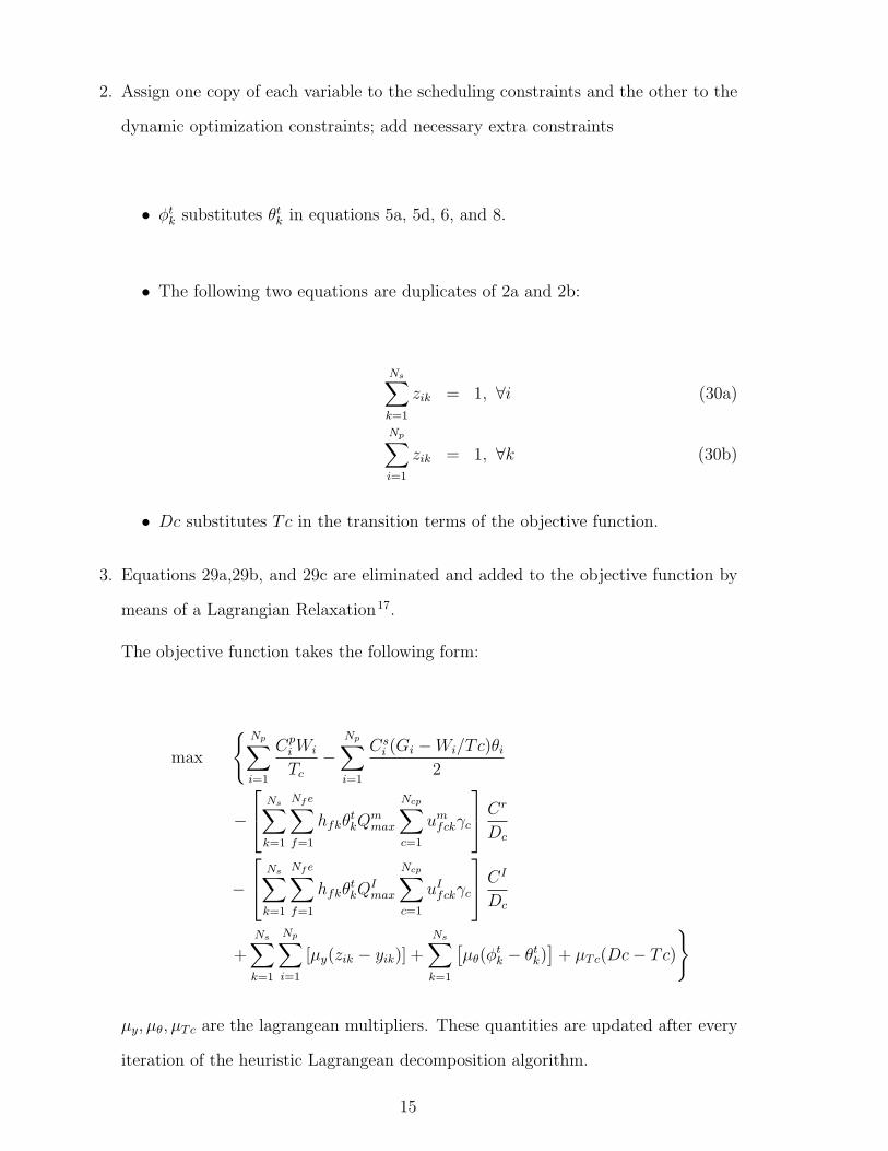
2. Assign one copy of each variable to the scheduling constraints and the other to the

dynamic optimization constraints; add necessary extra constraints

• φtk substitutes θt

k in equations 5a, 5d, 6, and 8.

• The following two equations are duplicates of 2a and 2b:

Ns∑

k=1

zik = 1, ∀i (30a)

Np∑i=1

zik = 1, ∀k (30b)

• Dc substitutes Tc in the transition terms of the objective function.

3. Equations 29a,29b, and 29c are eliminated and added to the objective function by

means of a Lagrangian Relaxation17.

The objective function takes the following form:

max

Np∑i=1

Cpi Wi

Tc

−Np∑i=1

Csi (Gi −Wi/Tc)θi

2

−

Ns∑

k=1

Nf e∑

f=1

hfkθtkQ

mmax

Ncp∑c=1

umfckγc

Cr

Dc

−

Ns∑

k=1

Nf e∑

f=1

hfkθtkQ

Imax

Ncp∑c=1

uIfckγc

CI

Dc

+Ns∑

k=1

Np∑i=1

[µy(zik − yik)] +Ns∑

k=1

[µθ(φ

tk − θt

k)]+ µTc(Dc− Tc)

µy, µθ, µTc are the lagrangean multipliers. These quantities are updated after every

iteration of the heuristic Lagrangean decomposition algorithm.

15

4. The formulation is decomposed into a scheduling subproblem and a control sub-

problem.

• Scheduling Subproblem.

max

Np∑i=1

Cpi Wi

Tc

−Np∑i=1

Csi (Gi −Wi/Tc)θi

2

+Ns∑

k=1

Np∑i=1

[µy(−yik)] +Ns∑

k=1

[µθ(−θt

k)]+ µTc(−Tc)

(31)

s.t.

Equations. 2a to 5c

• Control Subproblem

max

−

Ns∑

k=1

Nf e∑

f=1

hfckθtkQ

Imax

Ncp∑c=1

uIfckγc

CI

Dc

−

Ns∑

k=1

Nf e∑

f=1

hfkθtkQ

mmax

Ncp∑c=1

umfckγc

Cm

Dc

+Ns∑

k=1

Np∑i=1

[µy(zik)] +Ns∑

k=1

[µθ(φ

tk)

]+ µTc(Dc)

(32)

s.t.

Equations. 5d to 28, 30a and 30b

with variable yik substituted for zik

and variable θtk substituted for φt

k

16

6 Case Studies

In the following section three polymerization reaction examples are used to illustrate the

usefulness of the decomposition technique. The solution obtained using the full space (di-

rect solution) and the scheduling subproblem of the decomposed formulation are MINLPs

solved using DICOPT. The control subproblem of the decomposed formulation and the

problem used to generate heuristic lower bounds are NLPs solved using CONOPT3. All

models are written in GAMS and solved using a 2.0 GHz machine.

6.1 MMA polymerization

Process Description

The MMA polymerization system used in this paper is that described by Silva-Beard

et.al.22. The polymerization reactions take place in a CSTR. Table 1 shows the design

and operating parameters of the reactor. The mathematical model that describes the

bulk free-radical MMA polymerization using AIBN as the initiator is described below:

dCm

dt= −(kp + kfm)CmPo +

F (Cmin − Cin)

V(33)

dCI

dt= −kICI + fracFICIin − FCIV (34)

dT

dt=

(−∆H)kpCm

ρCp

P0 − UA

ρCpV(T − Tj) +

F (Tin − T )

V(35)

dD0

dt= (0.5Ktc + ktd)P

20 + kfmCmP0 − FD0

V(36)

dD1

dt= Mm(kp + kfm)CmP0 − FD1

V(37)

dTj

dt=

Fcw(Tw0 − Tj)

V0

+UA

ρCpwV0

(T − Tj); (38)

where

P0 =

√2f ∗CIkI

ktd + ktc

kr = Are−E/RT , r = p, fm, I, td, tc

17

Five different MMA grades are produced, where each grade corresponds to a different

steady state. Table 2 shows the values of the main process variables that correspond to

each steady state. Solutions using the full space and a using the decomposition heuristic

are easily computed with little computational effort. This example is included so the

decomposition approach is analyzed using a simple example, and the results are validated

against the solution found in the full solution space.

Results

In this section the results of the iterative heuristic decomposition technique are pre-

sented and compared against those obtained by solving the SSC model in full space (direct

solution). Our main interest is analyzing the performance of the decomposition technique

in terms of the optimal profit and the computational effort. Table 3 contains values of the

main decision variables for the solutions found with and without using the decomposition

technique. The values of the sequencing binary variables used to initialize both cases

corresponds to the sequence A → B → C → D → E. The initialization values of all

other decision variables are also identical between the direct and decomposed formulations.

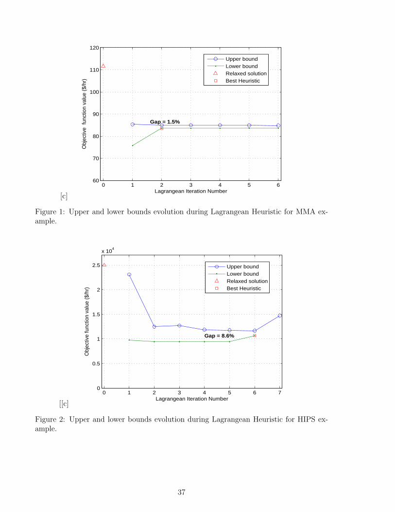
Figure 1 shows the evolution of the upper and lower bounds during the Lagrangean

iterative procedure. A drastic improvement in upper bounding from the relaxed solution

is observed. In fact a very tight upper bound is obtained in the iteration, and even slightly

improved in subsequent iterations. The heuristic lower bound obtained by fixing the bi-

nary variables of the original problem to their corresponding values for the scheduling

subproblem in the decomposed formulation reaches its maximum value after two itera-

tions. At this point the gap between bounds is approximately 1.5%. In fact, the algorithm

could be said to converge in two iterations with a tolerance of 2% for the gap between

bounds. For this illustrative example the algorithm is continued after two iterations to

show how the improvement stalls after that point.

It is important to say that the duplicated variables that allow the decomposition, namely,

18

cycle time, transition time, and sequencing variables, do not converge to the same values

during the algorithm, even though the optimal value of the decomposition (upper bound)

converges to the optimal of the original problem (lower bound). This has been reported in

previous works,14,23 and it is due to the effect of using the subgradient method for updat-

ing the Lagrange multipliers. This is not a serious problem for the heuristic method used

in this work, since the optimal value reported is always determined from the best lower

bound. This bound is obtained by fixing binary variables, and keeping all of the original

problem constraints. Therefore, the solution obtained represents a feasible solution to the

original, non-decomposed problem. The value of the upper bound is used only to certain

determined convergence of the algorithm.

Table 3 shows computational times and optimal solutions for the decomposed and di-

rect approaches (including all six iterations). The CPU solution time for the decomposed

formulation is 21 seconds lower than for the direct formulation, and the optimum found

is better. The solution time required using both techniques is relatively low (128 and

106 CPUs) in this illustrative example, but still a 16% reduction in the solution time is

achieved. Table 4 shows the size of the direct formulation and of each of the subproblems

involved in the decomposed formulation. This table includes the SSC formulation with

fixed binary variables, used for obtaining the heuristic lower bound. In this table the

increase in number of variables used for the decomposed formulation is evident. However,

in the decomposed formulation binary variables are only present in the scheduling sub-

problem, since the sequencing variables for the control problem are continuous as shown

in equation 29a. Therefore, in the decomposition technique the complicating integer vari-

ables are confined to a much smaller problem. From Table 4 one can see that the largest

portion of solution time for the decomposition algorithm is spent solving the NLP that

provides the lower bounds.

Comparison of optimal solutions.

19

The decomposition technique finds a better local optimum than the one found using

the full solution space. Notice how the direct formulation optimum corresponds to the

initial sequence provided to the solver. On the other hand, the decomposition results

show a very different sequence. The iterative nature of the heuristic decomposition tech-

nique, where Lagrange multipliers are updated in every iteration, allows for a different

local search every time. The profit of 83.6 $/hr is still a local optimum for one set of

values for the Lagrangian Multipliers.

Reference4 includes an extensive analysis of the behavior of different decision variables

for the isothermal version of the MMA model presented in this work. The findings in4 can

be applied to the comparison between the optimal profit for the direct approach and the

decomposed approach. Raw material, inventory costs and product prices are the same

as those used in4. Tables 5 and 6 show the values for the main decision variables for

the direct and decomposed solution. Both solution share one important characteristic.

Even though there is no upper bound on sales (all polymer produced is sold), all grades

are produced exactly to meet demand; not even grade E, which is the most profitable, is

produced more than it is demanded. This means that every extra hour that the cycle is

extended the inventory costs incurred are greater than the profit generated by the extra

production. In this scenario the cycle productivity, and the minimization of the time

spent in grade transitions becomes very important.

Figures 4 and 5 show the dynamic transitions for the direct and decomposed solutions.

The heuristic decomposition algorithm results in an optimal cycle characterized by faster

transitions and a shorter, more productive cycle. Figures 4 and 5 show that the longest

transition for the direct solution takes almost seven hours, while the longest transition for

the decomposed approach takes less than four. For the decomposed solution the optimizer

chooses transitions between non sequential grades (A to C, C to E, etc.). This avoids the

need for a long transition at the end of the cycle. On the other hand the direct solution

20

chooses transitions between sequential grades (A to B, B to C, etc.) but is forced to

make a very long transition (E to A) at the end of the cycle. The optimal trajectories

for the decomposed approach show that for a couple of grade transitions the manipulated

variable, namely, the initiator flow rate, is completely shut down for a while. This helps

in making the transitions cheaper since less initiator is wasted in off-spec material.

6.2 HIPS polymerization reactor

Process Description

A second example is included with the goal of exploring the performance of the pro-

posed approach in presence of a stronger nonlinear behavior and a larger problem. For

that purpose the HIPS polymerization system24 is employed. The polymerization is car-

ried out in a CSTR. Table 7 shows the design and operating parameters of the reactor.

The dynamic model of a CSTR where the non-isothermal high impact polymerization of

styrene takes place is given as follows:

• Initiator concentration.

dCi

dt=

QiCfi −QCi

V−KdCi (39)

• Monomer concentration.

dCm

dt=

Q

V(Cf

m − Cm)−KpCm(µor + µo

b) (40)

• Butadiene concentration.

dCb

dt=

Q

V(Cf

b − Cb)− Cb(Ki2Cr + Kfsµor + Kfbµ

ob) (41)

• Radicals concentration.

dCr

dt= −Q

VCr + 2f ∗KdCi − Cr(Ki1Cm + Ki2Cb) (42)

21

• Branched radicals concentration.

dCbr

dt= −Q

VCbr +Cb(Ki2Cr +Kfb(µ

or +µo

b))−Cbr(Ki3Cm +Kt(µor +µo

b +Cbr)) (43)

• Reactor temperature.

dT

dt=

Q

V(T f − T ) +

∆HrKpCm(µor + µo

b)

ρsCps

− UA(T − Tj)

ρsCpsV(44)

• Cooling jacket temperature.

dTj

dt=

Qw

Vc

(T fj − Tj) +

UA(T − Tj)

ρwCpwVc

(45)

• Zeroth moment live polymer.

dλop

dt= −Q

Vλo

p +Kt

2(µo

r)2 + (KfsCm + KfbCb)µ

or (46)

• First moment live polymer.

dλ1p

dt= −Q

Vλ1

p + Ktµ1rµ

or + (KfsCm + KfbCb)µ

1r (47)

• Zeroth moment dead polymer.

dµor

dt= −Q

Vµo

r + 2KioC3m + Ki1CrCm + CmKfs(µ

or + µo

b)

−(KpCm + Kt(µor + µo

b + Cbr) + KfsCm + KfbCb)µor + KpCmµo

r (48)

• First moment dead polymer.

dµ1r

dt= −Q

Vµ1

r − (KpCm + Kt(µor + µo

b + Cbr) + KfsCm + KfbCb)µ1r

+KpCm(µ1r + µo

r) (49)

22

• Zeroth moment butadiene.

dµob

dt= −Q

Vµo

b + Ki3CbrCm − (KpCm + Kt(µor + µo

b + Cbr)

+KfsCm + KfbCb)µob + KpCmµo

b (50)

• Number molecular weight distribution.

Mn =λ1

p + µ1r

λop + µo

r

(51)

Five different HIPS grades are produced, where each grade corresponds to a different

steady state. Table 8 shows the values of the main processes variables that correspond to

each steady state.

Results

The behavior of the lower and upper bounding of the algorithm is presented in Figure

2, and the optimal solution and key decision variable values are presented in Table 9.

From Figure 2, it is clear that there is a significant duality gap between upper and lower

bounding. Using this same heuristic algorithm for an oilfield planning problem, Van den

Heever et. al.2 found differences of up 13.2% between upper and lower bounds which are

similar in magnitude to the 8.6% present in the HIPS case study. From the same Figure,

one can observe that the behavior of the upper bound is not always decreasing between

sequential iterations. This behavior is normal when the Lagrange multipliers are updated

using the subgradient method2,14,23. Still there is an overall decrease of the upper bound

as iterations increase up to the sixth iteration. Lower bounds do not follow a specific

pattern, but this behavior is also expected since they are generated heuristically. After 6

iterations, the upper bound starts to deteriorate and the lower bounding problem becomes

infeasible, so the algorithm is stopped. Two important points observed from the results

in Table 9 are that the optimal value found by the decomposition approach is better than

the one found in the full solution space, and the computational time is 38.5% shorter. The

23

key characteristic of the decomposed formulation that leads to shorter solution times for

this example is the exclusion of integer variables from the control subproblem. In Table

10, one can see that although the control subproblem is almost as large as the complete

direct formulation, its repetitive solution took only 64% of the 1154 CPUs of solution time

for the whole decomposition algorithm. This is a much lower solution time per iteration

than the 1876 CPUs for the direct formulation.

There are important differences between the MMA and the HIPS cases just presented.

As problem size and complexity increase, the duality gap increases, but the benefits in

terms of computational time become more significant. The same decomposition and so-

lution methodology was used for the MMA case study and the HIPS case study, so the

differences in performance can be attributed to a larger problem size (see Table 10) with

stronger nonlinearities and nonconvexities in the HIPS case. Notice however, that the

optimal found by using the decomposition technique is better for both examples.

Comparison of optimal solutions.

Table 9 shows that the overall transition time for the optimal solution found by the

decomposition algorithm is less than that found by direct solution. Duration of transi-

tion times is key in obtaining a better hourly profit for the production cycle since they

represent an unproductive period of the cycle. The cyclic scheduling model has the key

feature of continuously depleting products so they are not kept until the end of the cy-

cle. Therefore, the order of production does not influence inventory costs. Being this the

case, the optimizer will always try to determine the sequence of production based on the

shortest of transitions that in turn renders higher hourly profits. Figure 6 and 7 show the

dynamic transitions of both solutions. The shapes of the transition profiles are similar,

but the longest transition for the decomposition algorithm takes six hours vs. almost

eight hours for the full space solution. The decomposition solution includes transitions

between grades that are not adjacent in terms of MWD, like transitions A2 to A4 and

24

A3 to Nm, as opposed to the sequence Nm → A1 → A2 → A3 → A4 chosen by the

optimizer using the full solution space. The solution found by means of the decomposi-

tion heuristic avoids the need for a very long and expensive transition between the end of

one cycle and the beginning of the next. This explains why the longest transition of the

decomposed solution is two hours shorter than the longest transition of the direct solution.

The values of some decision variables for both solutions are found in Tables 11 and

12. A common characteristic of both solutions is that the quantity of grade A3 produced

is much greater than what is demanded. The cyclic scheduling formulation used in this

work sets only a lower bound for production (demand must be satisfied) but sets no

upper bound, since it assumes that all polymer produced is sold. Grade A3 has the most

favorable price to inventory costs proportion (raw material costs are the same for all

grades), so it is easy to understand why most of the cycle is devoted to producing this

grade, while all other grades are only produced to meet the demands. Also, the cycle

resulting from the decomposed solution is shorter and more productive (total transition

duration is shorter).

6.3 HIPS polymerization reaction train

The previous examples were solved using full solution space and using the described de-

composition heuristic. The ultimate goal of the decomposition approach is not only to

reduce computational effort and time, but to provide a solution for problems that are

extremely difficult or even impossible to solve using the full space strategy. The following

case study provides an example of a system were we could not obtain a solution using the

full solution space.

Process Description

The system used for this case study is the High Impact Polystyrene free-radical bulk

polymerization system. The mathematical model describing the process is shown in the

25

previous case example. In the present example the reaction is not carried out in a single

CSTR but in a series of reactors25. As displayed in Figure 9, the typical industrial set-up

to carry out the HIPS polymerization reaction includes a CSTR, followed by a tubular

reactor, and a heat exchanger were the reaction is completed. To represent the process

without the complexities inherent in the modeling of tubular reactors, a mathematical

model consisting of 7 CSTRs is used. The first reactor of the model represents the CSTR

in the actual process; the following five CSTRs are used to model the tubular reactor,

and the last CSTR in the model represents the heat exchanger. Each CSTR is modeled

with a set of differential equations, equivalent to equations 39 - 45, 48, and 50. Table 13

shows the design parameters for the seven reactors of the model. The rest of the system

parameters can be read from Table 7. Four different HIPS grades are produced, where

each grade corresponds to a different steady state. Table 14 shows the values of the main

processes variables and parameters that correspond to each steady state.

Results and Discussion

Figure 3 shows the evolution of the upper and lower bounding as the Lagrangean it-

erations proceed. This figure shows what Guignard23 describes as a typical behavior of a

“good” case when the subgradient method is being used for updating the Lagrange mul-

tipliers: a “sawtooth” pattern in the Lagrangean value for the first iterations, followed by

a roughly monotonic improvement. The best lower bound, which corresponds to reported

optimal solution, is found rather quickly, in less than 10 iterations. However, since the

quality of the upper bound is improving considerably when this best lower bound is found,

the algorithm is kept running. From iteration 30 onwards, the quality of the upper bound

improves very slowly, while the lower bound keeps cycling among a few values. After

39 iterations the algorithm is stopped. At this point there is a 8.5% difference between

upper and lower bounding. Once again, the best lower bound is reported as the best

solution since all constraints of the original problem are satisfied, and therefore it is the

26

best feasible solution found by the algorithm. The optimal solution is reported in Table

15. Values of the most important decision variables for the optimal solution are found in

Table 16. One of the key features of the solution is that the production wheel is carried

out so that three grades (N,A, B) are produced to satisfy their demands (as required by

the formulation) , and only grade C, which is the most profitable product, is produced

over its demanded quantity (remember that there is no upper bound on production).

Transition times are not compared against any other solution, but from previous analysis

they are expected to be made as short as possible to achieve a productive manufacturing

cycle.

Table 17 shows the size of the problem. In this example the most expensive subprob-

lem is the control subproblem, in contrast to the heuristic subproblem, as in the previous

examples. The extra complexity in the dynamic optimization of a train of reactors instead

of just one CSTR is the main reason. Notice, once again, that the control subproblem

does not include integer variables. The copy of the sequencing variables used in this sub-

problem is allowed to have continuous values between 0 and 1. The final value for the

sequencing variables of the scheduling and the control subproblem for the last iteration of

the decomposition algorithm are shown in Table 18. The same Table shows the values for

the other duplicated variables for both subproblems. The values of the decision variables

shown in this Table are not the optimal values found. The heuristic optimal solution is

found in iteration number seven. Nevertheless, it is important to analyze the values of

these variables in the last iteration in order to show how the algorithm deals with the

duplicity of the variables copied in order to achieve the decomposition. The sequencing

variables, yik for the scheduling subproblem are binary variables, while their copies in the

control subproblem zik are allowed to have continuous values between 0 and 1. This fact is

important since it is the key feature that reduces computational effort in the decomposi-

tion heuristic when compared against the direct solution. Notice that in the last iteration

the values of both sets of variables are identical in some cases and almost the same for

27

others. In the worst cases the continuous variables have values of more than 0.99 or less

than 0.01. This was achieved by the term in the objective function that penalizes the

differences between copies of sequencing variables. Although the variables in the control

subproblem are continuous they are forced by the algorithm to adopt values of exactly or

very close to 0 and 1, so that the originally continuous variables behave very much like

binary variables without the added complexity of this type of variables. Moreover, the

sequence in the control subproblem is virtually the same as in the scheduling subproblem.

The case is not the same for the transition durations and the cyclic time. Both sub-

problems still do not have the same values for the copied variables. These values might

have eventually converged, but the time required for this convergence was considered not

practical. Moreover, there is no mathematical guarantee that all duplicated variables will

converge, even if the gap between upper and lower bound is minimized14. The objective

of the algorithm of finding an optimal solution by heuristic lower bounding, while obtain-

ing reasonable, well behaved upper bounds, is considered achieved after the determined

number of iterations. This conclusion is validated by previous examples where a direct

solution was available.

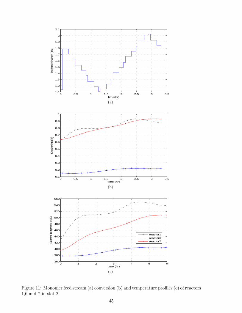
Dynamic behaviors of grade transitions in reactors 1,6 and 7 are shown in Figures

10-13. The profiles of these reactors correspond to the outlet of the actual process equip-

ment: reactor 1 of the model is the actual CSTR, reactor 6 represents the last section

of the actual tubular reactor, and reactor 7 of the model represents the process heat ex-

changer where the reaction is completed. Since the manipulated variable (monomer flow

rate) is the same for the seven reactors at any given moment, there is only one dynamic

profile per slot. The monomer flow rate during all grade transitions seems to follow the

same pattern. The flow rate is decreased during the first part of the transition and then

increased towards its steady state value. Such initial decrease in flow rate decreases the

total cost of the transition since less monomer is wasted as off spec product. From Figures

10-13 one can see that in reactor one the controlled variables undergo small changes in

28

magnitude as they transition from one steady state to the next. This reactor has the low-

est conversion values, so the operating temperatures are the lowest. In the initial stage

the reaction rate is slower than in the rest of the reactors, and therefore the action of

the manipulated variable does not have dramatic effects on the controlled variables. In

contrast, the temperature and conversion inside reactor six, exhibit very fast responses

to changes in the monomer flow rate. Recall that this reactor represents the last segment

of the tubular reactor, which is modeled as a small CSTR. Since the volume is smaller

than in the other two reactors (the residence time is shorter) and the temperatures are

high, it is not surprising that the dynamic responses in this reactor are faster. Reactor 7

is similar in size to reactor 1, but its operating temperature is higher, so larger changes

in conversion are carried out during grade transition. Duration of dynamic transitions in

the HIPS reactor train is similar to dynamic transitions in the previous HIPS example,

in which polymerization took place in only one CSTR. The longest transition for both

examples takes around six hours. This means that the addition of a series of reactors

instead of just one reactor should not result in a significant increase in transition costs in

terms of wasted off spec material.

This last example illustrates how the decomposition heuristic described in this work

represents a practical alternative for solving SSC problems, especially as they grow in

size, nonlinearity and nonconvexity. In previous examples, although the computational

effort of the decomposition approach was reduced, the solution in full space was available.

However, in this last example it was impossible to find a solution in full space, using the

same outer approximation algorithm (DICOPT) that was successfully used in previous

examples. When trying to obtain a solution without the decomposition approach, the

MINLP problem invariably became infeasible.

29

7 Conclusions

The Lagrangean Decomposition methodology as presented by Guignard and Kim1 was

used to reformulate the SSC problem10,4. A solution methodology very similar to the

one presented by Van den Heever et. al.2 was used. According to this methodology the

decomposed formulation is used to generate an upper bound and a heuristic procedure is

used to generate a lower bound. The decomposition approach was successful for solving

the SSC problem in the MMA example and in the HIPS polymerization system, using

one CSTR and seven CSTRs. In the first two cases the optimal solution found by the

decomposition approach was better than the solution obtained in the full space. Since

both systems are highly nonlinear the better profit found by the decomposition approach

is attributed to an increased number of local searches driven by the repetitive solution of

the SSC problem in different iterations. In these two examples, the computational effort

required by the decomposition heuristic is lower than the computational effort required by

the direct solution (solution in full space). The third problem was only solvable using the

decomposition heuristic. The present work does not prove that the solution to the SSC

problem in the HIPS reactor train example cannot be obtained without the decomposition.

However, it does show is that if such a direct solution is available, the effort required to

obtain it becomes unpractical.

Future directions of our research include the simultaneous scheduling and control of

even larger problems, as well as the simultaneous design, scheduling, and control of poly-

merization systems. The Lagrangean Decomposition Heuristic described in this paper

could prove to be very useful in both cases.

30

Table 1: Design and Operation Parameters for the MMA Polymerization Reactors

F = 1.0 m3/h Mm = 100.12 kg/kgmolFI = 0.0032 m3/h f ∗ = 0.58Fcw = 0.1588 m3/h R = 8.314 kJ/(kgmol· K)Cmin = 6.4678 kgmol/m3 −∆H = 57800 kJ/kgmolCIin = 8.0 kgmol/m3 Ep = 1.8283 x 104 kJ/kgmolTin = 350 K EI = 1.2877 x 105 kJ/kgmolTw0 = 293.2 K Efm = 7.4478 x 104 kJ/kgmolU = 720 kJ/(h· K· m2) Etc = 2.9442 x 103 kJ/kgmolA = 2 m2 Etd = 2.9442 x 103 kJ/kgmolV = 0.1 m3 Ap = 1.77 x 109 m3/(kgmol· h)V0 = 0.02 m3 AI = 3.792 x 1018 1/hρ = 866 kg/m3 Afm = 1.0067 x 1015 m3/(kgmol· h)ρw = 1000 kg/m3 Atc = 3.8223 x 1010 m3/(kgmol· h)Cp = 2 kJ/(kg · K) Atd = 3.1457 x 1011 m3/(kgmol· h)Cpw = 4.2 kJ/(kg · K)

Table 2: Steady States and grade information of the MMA polymerization reactor

State A State B State C State D State ECm (kmol/m3) 5.5542 5.9653 6.0842 6.2341 6.3245Treactor (K) 362 351 348 344 342X% 14 8 6 4 2MWD (kg/kmol) 15000 25000 30000 39000 48000FI (m3/hr) 2.5x10−3 3.2x10−3 2.9x10−3 2x10−3 1.1x10−3

Demand (kg/hr) 0.8 0.7 1 0.8 0.6Inv. Cost ($/hr-kg) 0.10 0.12 0.12 0.15 0.15Mono. Cost ($/ltfeed) 10 10 10 10 10Init. Cost ($/ltfeed) 500 500 500 500 500

Table 3: Direct and Lagrangean solutions for MMA example

Algorithm Obj. [$/hr] Opt. Sequence Cycle [hr] Trans. [hr] CPU [s]Direct 81.6 A → B → C → D → E 149.4 14.9 128

Decomposed 83.6 B → A → C → E → D 139.9 14.0 107

Table 4: Problem Size for Direct and Decomposed Solution for MMA example. Percentof CPU time represents the time spent in each subproblem of the decomposed solution

Subproblem Cont. variables Discrete Variables % CPU TimeMMA Direct 4927 25

MMA Scheduling Subproblem 57 25 0.8MMA Control Subproblem 4902 none 42MMA Heuristic Subproblem 4927 none 57.2

31

Table 5: Simultaneous scheduling and control results in full space, for grade transitionin a MMA polymerization CSTR. The objective function value is $ 81.6/hr and 149 h oftotal cycle time.

Product Process T [h] production [kg] Trans T [h] T start[h] T end [h]A 29.88 119.51 2.83 0 32.70B 20.91 104.57 1.60 62.19 55.22C 37.35 149.39 1.99 101.24 94.56D 23.90 119.51 1.69 127.57 120.15E 22.41 89.63 6.83 127.57 149.39

Table 6: Simultaneous scheduling and control results using decomposition heuristic, forgrade transition in a MMA polymerization CSTR. The objective function value is $83.6/hr and 140 h of total cycle time.

Product Process T [h] production [kg] Trans T [h] T start[h] T end [h]B 19.58 97.89 3.22 0 22.80A 27.97 111.88 3.18 22.80 53.95C 34.96 139.85 2.76 53.95 91.67E 20.98 83.91 1.52 91.67 114.17D 22.38 111.88 3.30 114.17 139.85

32

Table 7: Nominal parameter values for an industrial scale HIPS CSTR.

Parameter Value Units Parameter Value Units

Q 1.1411813934 L/s T fj 294 K

Cfi 0.9814814815 mol/L T f 333 K

Qi 0.0015 L/s Qw 1 L/s

Cfm 8.6310347459 mol/L Cf

b 1.0547874055 mol/L

V 9450 L Vc 2000 L

f ∗ 0.57 ∆Hr 69919.56 J/mol

ρs 0.915 kg/L Cps 1647.265 J/(kg-K)

ρw 1 kg/L Cpw 4045.7048 J/(kg-k)

A 19.5 m2 U 80 J/(s-K-m2)

R 1.9858 cal/(mol-K) Ai0 1.1x105 L2/(mol2-s)

Ei0 27340 cal/mol Ad 9.1x1013 1/s

Ed 29508 cal/mol Ai1 1x107 L/(mol-s)

Ei1 7067 cal/mol Ai2 2x106 L/(mol-s)

Ei2 7067 cal/mol Ai3 1x107 L/(mol-s)

Ei3 7067 cal/mol Ap 1x107 L/(mol-s)

Ep 7067 cal/mol At 1.7x109 L/(mol-s)

Et 843 K Afs 6.6x107 L/(mol-s)

Efs 14400 cal/mol Afb 2.3x109 L/(mol-s)

Efb 18000 cal/mol

Table 8: Steady States and grade information of the HIPS polymerization reactor

State Nm State A1 State A2 State A3 State A4Cm 6.0725 6.6229 6.0842 8.5536 8.600Treactor 389 381 348 330 320X% 30 23 10 1 0.5MWD 118000 125000 148000 343000 489000Qw [L/s] 1.0 0.5 0.1 0.1 0.5Demand [kg/hr] 50 60 65 70 60Price [$/kg] 3.2 4.3 4.5 5.0 5.5Inv. Cost [$/hr-kg)] 0.15 0.20 0.15 0.10 0.25Mono. Cost [$/ltfeed] 1 1 1 1 1Init. Cost [$/ltfeed] 10 10 10 10 10

Table 9: Direct and Lagrangan solutions for HIPS example

Algorithm Obj. [$/hr] Opt. Sequence Cycle [hr] Trans. [hr] CPU [s]Direct 10500.1 Nm → A1 → A2 → A3 → A4 88.4 12.6 1876

Decomposed 10568.2 A2 → A4 → A3 → Nm → A1 87.1 12.2 1154

33

Table 10: Problem Size for Direct and Decomposed Solution for HIPS example. Percentof CPU time represents the time spent in each subproblem of the decomposed solution

Subproblem Cont. variables Discrete Variables % CPU TimeHIPS Direct 13452 25

HIPS Scheduling Subproblem 62 25 0.07HIPS Control Subproblem 13422 none 35.62HIPS Heuristic Subproblem 13452 none 64.31

Table 11: Simultaneous scheduling and control results in full space, for grade transitionin a HIPS polymerization CSTR. The objective function value is $ 10500/hr and 88.4 hof total cycle time.

Product Process T [h] production [kg] Trans T [h] T start[h] T end [h]Nm 2.00 4421.3 0.98 0 2.18A1 1.44 5305.6 1.80 2.18 5.42A2 1.56 5747.8 1.65 5.42 8.63A3 70.18 2.5915e5 0.50 8.63 79.30A4 1.44 5305.6 7.69 79.30 88.43

Table 12: Simultaneous scheduling and control results using decomposition heuristic,for grade transition in a HIPS polymerization CSTR. The objective function value is $10568/hr and 87.1 hrs of total cycle time.

Product Process T [h] production [kg] Trans T [h] T start[h] T end [h]A2 1.53 5659.87 2.02 0 3.55A4 1.42 5659.87 1.39 3.55 6.35A3 69.34 2.5607e5 6.01 6.35 81.70Nm 1.18 4353.75 0.98 81.70 83.86A1 1.42 5224.59 1.80 83.86 87.08

Table 13: Design parameters for the seven reactors of the HIPS reaction train.Qcw standsfor cooling water flow rate.

Reactor Volume [L] Jacket Volume [L] Qcw [L/s] Heat-Transfer Area [m2]1 6000 1200 0.1311 11.7182 900 180 1.0 1.75783 1000 200 1.0 1.95314 650 130 1.0 1.26955 1000 200 1.0 1.95316 1000 200 1.0 1.95317 5000 1000 1.0 9.5676

34

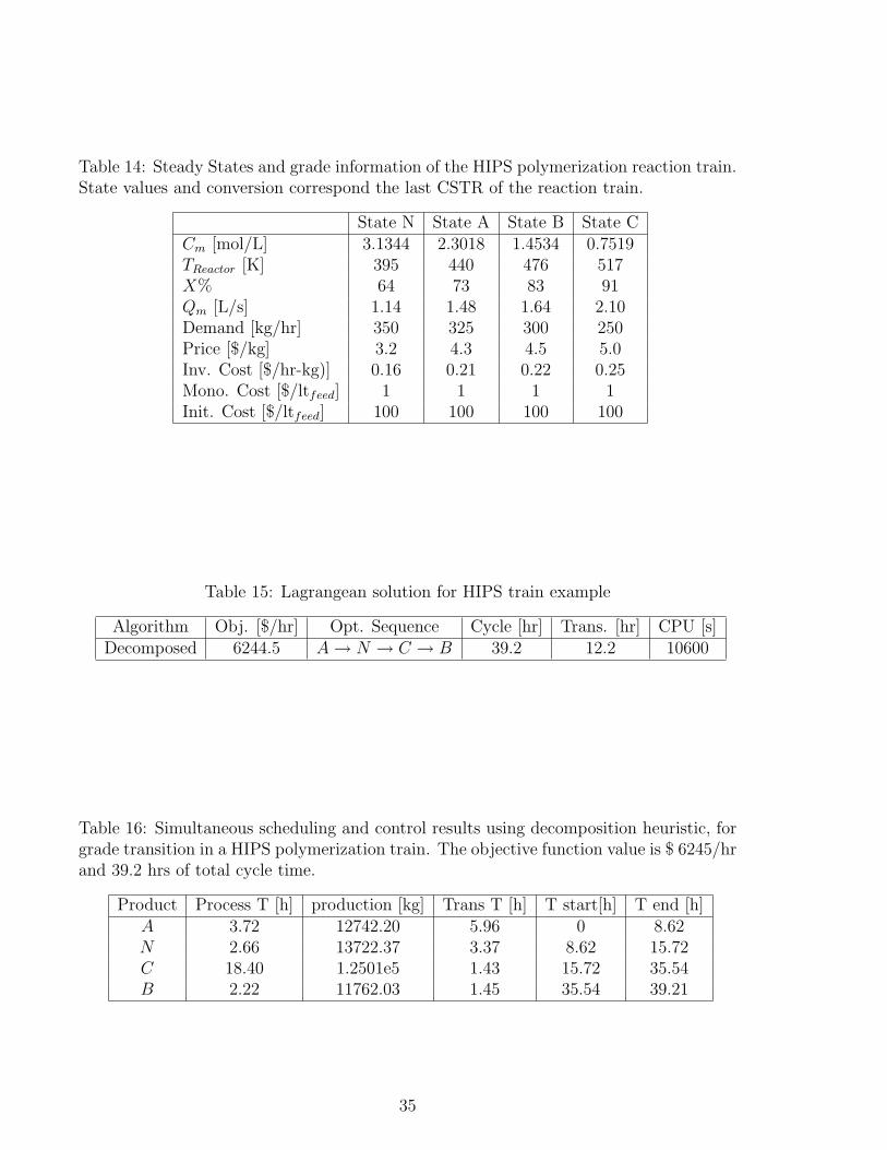
Table 14: Steady States and grade information of the HIPS polymerization reaction train.State values and conversion correspond the last CSTR of the reaction train.

State N State A State B State CCm [mol/L] 3.1344 2.3018 1.4534 0.7519TReactor [K] 395 440 476 517X% 64 73 83 91Qm [L/s] 1.14 1.48 1.64 2.10Demand [kg/hr] 350 325 300 250Price [$/kg] 3.2 4.3 4.5 5.0Inv. Cost [$/hr-kg)] 0.16 0.21 0.22 0.25Mono. Cost [$/ltfeed] 1 1 1 1Init. Cost [$/ltfeed] 100 100 100 100

Table 15: Lagrangean solution for HIPS train example

Algorithm Obj. [$/hr] Opt. Sequence Cycle [hr] Trans. [hr] CPU [s]Decomposed 6244.5 A → N → C → B 39.2 12.2 10600

Table 16: Simultaneous scheduling and control results using decomposition heuristic, forgrade transition in a HIPS polymerization train. The objective function value is $ 6245/hrand 39.2 hrs of total cycle time.

Product Process T [h] production [kg] Trans T [h] T start[h] T end [h]A 3.72 12742.20 5.96 0 8.62N 2.66 13722.37 3.37 8.62 15.72C 18.40 1.2501e5 1.43 15.72 35.54B 2.22 11762.03 1.45 35.54 39.21

35

Table 17: Problem Size for Direct and Decomposed Solution for HIPS train example.Percent of CPU time represents the time spent in each subproblem of the decomposedsolution

Subproblem Cont. variables Discrete Variables % CPU TimeHIPS Scheduling Subproblem 46 16 0.03

HIPS Control Subproblem 22678 none 67.76HIPS Heuristic Subproblem 22702 none 32.21

Table 18: Value of the duplicated variables in the last Lagrangean iteration. The bestupper bound is found in this last iteration, corresponding to an objective value of $ 6823.58/hr. Binary variables, and their continuous equivalents in the control subproblem, notshown have a value of 0.

Variable Scheduling Subproblem Control SubproblemyB1 1 -yA2 1 -yN3 1 -yC4 1 -zB1 - 0.994zA2 - 0.994zN3 - 1.000zC4 - 1.000zA1 - 0.006zB2 - 0.006θt1 0.50 -

θt2 0.50 -

θt3 0.50 -

θt4 0.50 -

φt1 - 1.43

φt2 - 6.60

φt3 - 3.31

φt4 - 1.43

Tc 16.634 -Dc 443.486 -

36

[c]

0 1 2 3 4 5 660

70

80

90

100

110

120

Lagrangean Iteration Number

Obj

ectiv

e fu

nctio

n va

lue

($/h

r)

Gap = 1.5%

Upper boundLower boundRelaxed solutionBest Heuristic

Figure 1: Upper and lower bounds evolution during Lagrangean Heuristic for MMA ex-ample.

[[c]

0 1 2 3 4 5 6 70

0.5

1

1.5

2

2.5

x 104


Obj

ectiv

e fu

nctio

n va

lue

($/h

r)

Gap = 8.6%


Figure 2: Upper and lower bounds evolution during Lagrangean Heuristic for HIPS ex-ample.

37

[c]

0 5 10 15 20 25 30 35 400

0.5

1

1.5

2

2.5

x 104


Obj

ectiv

e fu

nctio

n va

lue

($/h

r)

Gap = 8.5%


Figure 3: Upper and lower bounds evolution during Lagrangean Heuristic for HIPS ex-ample.

38

0 1 2 3 4 5 6 70

1

2

3

4

5

6

7x 10

−3

time(h)

Initia

tor f

lowr

ate

(lt/m

in)

slot1slot2slot3slot4slot5

(a)

0 1 2 3 4 5 6 71

1.5

2

2.5

3

3.5

4

4.5

5x 10

4

time (h)

MW

D


(b)

0 1 2 3 4 5 6 7340

345

350

355

360

365

time(h)

Reac

tor T

empe

ratu

re (K

)


(c)

Figure 4: Dynamic transitions for the MMA example obtained by direct solution: (a)Manipulated variable (b) MWD (c) Reactor Temperature

39

0 0.5 1 1.5 2 2.5 3 3.50

1

2

3

4

5

6

7x 10

−3

time(h)

Initia

tor f

lowr

ate

(lt/m

in)


(a)

0 0.5 1 1.5 2 2.5 3 3.51

1.5

2

2.5

3

3.5

4

4.5

5x 10

4

time (h)

MW

D


(b)

0 0.5 1 1.5 2 2.5 3 3.5340

345

350

355

360

365

time(h)

Reac

tor T

empe

ratu

re (K

)


(c)

Figure 5: Dynamic transitions for the MMA example obtained by Lagrange Heuristic:(a) Manipulated variable (b) MWD (c) Reactor Temperature

40

0 1 2 3 4 5 6 7 80

0.5

1

1.5

2

2.5

3

3.5

time(h)

Cool

ing

wate

r flo

wrat

e (lt

/min

)


(a)

0 1 2 3 4 5 6 7 81

1.5

2

2.5

3

3.5

4

4.5

5

5.5

6x 10

5

time (h)

MW

D


(b)

0 1 2 3 4 5 6 7 8320

330

340

350

360

370

380

390

time(h)

Reac

tor T

empe

ratu

re (K

)


(c)

Figure 6: Dynamic transitions for the HIPS example obtained by direct solution: (a)Manipulated variable (b) MWD (c) Reactor Temperature

41

STYRENE

STYRENEINITIATOR

RECOVEREDSTYRENE

CSTR

TUBULARREACTOR

HEATEXCHANGER

GRIDING

MONOMERRECOVERYSYSTEM

R2 R3

DV1

DV2

R1

(a)

1 2 3 4 5 6 7

(b)

Figure 8:

Figure 9: (a) Flowsheet of the HIPS plant, (b) Approximation of the HIPS plant by aset of 7 series-conneced CSTRs. The dashed box stands for the 5 CSTRs employed forapproximating the steady-state behavior of the R2 tubular reactor.

42

0 1 2 3 4 5 6 70

0.5

1

1.5

2

2.5

3

time(h)

Cool

ing

wate

r flo

wrat

e (lt

/min

)


(a)

0 1 2 3 4 5 6 7 81

1.5

2

2.5

3

3.5

4

4.5

5

5.5

6x 10

5

time (h)

MW

D


(b)

0 1 2 3 4 5 6 7320

330

340

350

360

370

380

390

time(h)

Reac

tor T

empe

ratu

re (K

)


(c)

Figure 7: Dynamic transitions for the HIPS example obtained by Lagrange Heuristicsolution: (a) Manipulated variable (b) MWD (c) Reactor Temperature

43

0 1 2 3 4 5 60.8

1

1.2

1.4

1.6

1.8

2

time(hr)

Mon

omer

flowr

ate

(lt/s

)

(a)

0 1 2 3 4 5 60.1

0.2

0.3

0.4

0.5

0.6

0.7

0.8

time (hr)

Conv

ersio

n (%

)

(b)

0 1 2 3 4 5 6320

340

360

380

400

420

440

460

480

time (hr)

Reac

tor T

empe

ratu

re (K

)

reactor1reactor6reactor7

(c)

Figure 10: Monomer feed stream (a) conversion (b) and temperature profiles (c) of reactors1,6 and 7 in slot 1.

44

0 0.5 1 1.5 2 2.5 3 3.51.1

1.2

1.3

1.4

1.5

1.6

1.7

1.8

1.9

2

2.1

time(hr)

Mon

omer

flowr

ate

(lt/s

)

(a)

0 0.5 1 1.5 2 2.5 3 3.50.1

0.2

0.3

0.4

0.5

0.6

0.7

0.8

0.9

1

time (hr)

Conv

ersio

n (%

)

(b)

0 1 2 3 4 5 6360

380

400

420

440

460

480

500

520

540

560

time (hr)

Reac

tor T

empe

ratu

re (K

)


(c)


45

0 0.5 1 1.51.5

1.6

1.7

1.8

1.9

2

2.1

2.2

2.3

time(hr)

Mon

omer

flowr

ate

(lt/s

)

(a)

0 0.5 1 1.50.2

0.3

0.4

0.5

0.6

0.7

0.8

0.9

1

time (hr)

Conv

ersio

n (%

)

(b)

0 0.5 1 1.5400

450

500

550

time (hr)

Reac

tor T

empe

ratu

re (K

)


(c)


46

0 0.5 1 1.51.1

1.2

1.3

1.4

1.5

1.6

1.7

1.8

1.9

2

2.1

time(hr)

Mon

omer

flowr

ate

(lt/s

)

(a)

0 0.5 1 1.50.1

0.2

0.3

0.4

0.5

0.6

0.7

0.8

0.9

time (hr)

Conv

ersio

n (%

)

(b)

0 0.5 1 1.5390

400

410

420

430

440

450

460

470

480

490

time (hr)

Reac

tor T

empe

ratu

re (K

)


(c)


47

References

[1] Guignard M., Kim S.. Lagrangean Decomposition: A model yielding Stronger La-

grangean Bounds Mathematical Programming. 1987;39:215-228.

[2] Van-Heerden S.A., Grossmann I.E., Vasantharajan S., Edwards K.. A Lagrangean

Decomposition Heuristic for the Design and Planning of Offshore Hydrocarbon

Field Infrastructures with Complex Economic Objectives Ind. Eng. Chem. Res..

2001;40:2857-2875.

[3] Mishra B.V., Mayer E., Raisch J., Kienle A.. Short-Term Scheduling of Batch

Processes. A Comparative Study of Different Approaches Ind. Eng. Chem. Res..

2005;44:4022-4034.

[4] Terrazas-Moreno S., Flores-Tlacuahuac A., Grossmann I.E.. Simultaneous Cyclic

Scheduling and Optimal Control of Polymerization Reactors Submitted for revision.

2006.

[5] Mahadevan R., Doyle F.J. III, Allcock A.C.. Control-Relevant Scheduling of Polymer

Grade Transitions AICHE J.. 2002;48(8):1754-1764.

[6] Feather D., Harrell D., Liberman R., Doyle F.J.. Hybrid Approach to Polymer Grade

Transition Control AICHE J.. 2004;50(10):2502-2513.

[7] Prata A., Oldenburg J., Marquardt W., R. Nystrom A. Kroll. Integrated Scheduling

and Dynamic Optimization of Grade Transitions for a Continuous Polymerization

Reactor Submitted for revision. .

[8] Nystrom R.H., Franke R., I.Harjunkoski , A.Kroll . Production Campaign Planning

including Grade Transition Sequencing and Dynamic Optimization Comput. Chem.

Eng.. 2005;29(10):2163-2179.

[9] Nystrom R.H., I.Harjunkoski , A.Kroll . Production Optimization for continuously

48

operated processes with optimal operation and scheduling of multiple units Comput.

Chem. Eng.. 2006;30:392-406.

[10] Flores-Tlacuahuac A., Grossmann I.E.. Simultaneous Cyclic Scheduling and Control

of a Multiproduct CSTR Ind. Eng. Chem. Res.. 2006;45(20):6698-6712.

[11] Biegler L.T.. Optimization strategies for complex process models Advances in Chem-

ical Engineering. 1992;18:197-256.

[12] deMatta R.. A Lagrangean decomposition solution to a single line multiproduct

scheduling problem European Journal of Operational Research. 1994;79:25-37.

[13] Wu D., Ierapetritou M.G.. Decomposition approaches for the efficient solution of

short-term scheduling problems Comput. Chem. Eng.. 2003;27:1261-1276.

[14] Wu D., Ierapetritou M.. Lagrangean decomposition using an improved Nelder-Mead

approach for Lagrangean multiplier update Comput. Chem. Eng.. 2003;27:1261-1276.

[15] Finlayson B.. Nonlinear Analysis in Chemical Engineering. New York: McGraw-Hill

1980.

[16] Villadsen , J. , M.Michelsen . Solution of Differential Equations Models by Polynomial

Approximation. Prentice-Hall 1978.

[17] Fisher M.L. The Lagrangean Relaxation Method for Solving Integer Programming

Problems Management Science. 1981;27(1):1.

[18] Guignard M.. Lagrangean Relaxation: A Short Course Belg. J. OR.: Special Issue

Francoro. 1995;35:3.

[19] Geoffrion A.M.. Lagrangean Relaxation for Integer Programming Math. Program.

Study 2. 1974;2:82-114.

[20] Fisher M.L.. An Application Oriented Guide to Lagrangian Relaxation Interfaces.

1985;15(2):10.

49

[21] Michelon P., Maculan N.. Lagrangean Decompostion for Integer Nonlinear Program-

ming with Linear Constraints Mathematical Programming. 1991;52:203-313.

[22] Silva-Beard S., Flores-Tlacuahuac A.. Effects of Process Design/Operation on the

Steady-State Operability of a Methyl-Methacrylate Polymerization Reactor Ind. Eng.

Chem. Res.. 1999;38:4790-4804.

[23] Guignard M.. Lagrangean Relaxation Top. 2003;11(2):151-228.

[24] Flores-Tlacuahuac A., Verazaluce-Garcıa J.C., Saldıvar-Guerra E.. Steady-State

Nonlinear Bifurcation Analysis of a High Impact Polystyrene Continuous Stirred

Reactor Ind. Eng. Chem. Res.. 2000;39:1972-1979.

[25] Flores-Tlacuahuac A., Biegler L.T., Saldıvar-Guerra E.. Dynamic Optimization

of HIPS Open-Loop Unstable Polymerization Reactors Ind. Eng. Chem. Res..

2005;44:2659-2674.

50

Appendix

The indices, decision variables and system parameters used in the SSC MIDO problem

formulation are as follows:

1. Indices

Products i, p = 1, . . . Np

Slots k = 1, . . . Ns

Finite elements f = 1, . . . Nfe

Collocation points c, l = 1, . . . Ncp

System states n = 1, . . . Nx

Manipulated variables m = 1, . . . Nu

2. Decision variables

yik Binary variable to denote if product i is assigned to slot k

zik Copy of yik

pk Processing time at slot k

tek Final time at slot k

tsk Start time at slot k

tfck Time at finite element f and collocation point c of slot k

Gi Production rate

Tc Cyclic time [h]

Dc Copy of Tc

xnfck n-th system state in finite element f and collocation point c of slot k

xnflk Value of n-th state derivative with respect to time in finite element f

and collocation point l of slot k

umfck m-th manipulated variable in finite element f and

collocation point c of slot k

51

Wi Amount produced of each product [kg]

θik Processing time of product i in slot k

θtk Transition time at slot k

φtk Copy of θt

k

Θi Total processing time of product i

xno,fk n-th state value at the beginning of the finite element f of slot k

xnk Desired value of the n-th state at the end of dynamic transition of slot k

umk Desired value of the m-th manipulated variable at the end of dynamic

transition of slot k

xnin,k n-th state value at the beginning of dynamic transition of slot k

unin,k m-th manipulated variable value at the beginning of dynamic transition

of slot k

Xfck Conversion in finite element f and collocation point c of slot k

MWDfck Molecular Weight Distribution in finite element f

and collocation point c of slot k

3. Parameters

Np Number of products

Ns Number of slots

Nfe Number of finite elements

Ncp Number of collocation points

Nx Number of system states

Nu Number of manipulated variables

52

Di Demand rate [kg/h]

Cpi Price of products [$/kg]

Csi Cost of inventory [$/kg-hr]

Cr Cost of raw material [$/lt of feed solution]

CI Cost of initiator [$/lt of feed solution]

hfk Length of finite element f in slot k

Ωcc Matrix of Radau quadrature weights

xnk Desired value of the n-th system state at slot k

umk Desired value of the m-th manipulated variable at slot k

θmax Upper bound on processing time

xnss,i n-th state value at steady state of product i

umss,i m-th manipulated variable value of product i

F oi Feed stream volumetric flow rate at steady state for grade i

MWmonomer Monomer molecular weight [kg/kmol]

Xss,i Desired conversion degree of grade i

MWDss,i Desired molecular weight distribution of grade i

xnmin, x

nmax Minimum and maximum value of the state xn

ummin, u

mmax Minimum and maximum value of the manipulated variable um

xntol Maximum absolute value for state derivatives at the end of dynamic

transition

xntol Maximum absolute deviation from desired final value, allowable for

state variable xn at the end of dynamic transition

ufcont Maximum absolute change for um between finite elements

uccont Maximum absolute change for um between collocation points

γc Roots of the Lagrange orthogonal polynomial

Qmmax Maximum monomer flow rate [lt/hr]

QImax Maximum initiator flow rate [lt/hr]

53

a lagrangean heuristic approach for the simultaneous...

Documents