a new interpolation approach and corresponding instance
TRANSCRIPT

1
A New Interpolation Approach
and Corresponding Instance-Based Learning
Shiyou Lian
Xi’an Shiyou University, Xi’an, China
Abstract
Starting from finding approximate value of a function, introduces the measure of
approximation-degree between two numerical values, proposes the concepts of "strict
approximation" and "strict approximation region", then, derives the corresponding
one-dimensional interpolation methods and formulas, and then presents a calculation model
called "sum-times-difference formula" for high-dimensional interpolation, thus develops a
new interpolation approach ADB interpolation. ADB interpolation is applied to the
interpolation of actual functions with satisfactory results. Viewed from principle and effect,
the interpolation approach is of novel idea, and has the advantages of simple calculation,
stable accuracy, facilitating parallel processing, very suiting for high-dimensional
interpolation, and easy to be extended to the interpolation of vector valued functions.
Applying the approach to instance-based learning, a new instance-based learning method
learning using ADB interpolation is obtained. The learning method is of unique technique,
which has also the advantages of definite mathematical basis, implicit distance weights,
avoiding misclassification, high efficiency, and wide range of applications, as well as being
interpretable, etc. In principle, this method is a kind of learning by analogy, which and the
deep learning that belongs to inductive learning can complement each other, and for some
problems, the two can even have an effect of “different approaches but equal results” in big
data and cloud computing environment. Thus, the learning using ADB interpolation can also
be regarded as a kind of “wide learning” that is dual to deep learning.
Keywords Approximation-Degree; Interpolation; Strict Approximation;
Sum-Times-Difference Formula; Instance-Based Learning; Wide Learning
1 Introduction
Instance-based learning[1,2]
is also called nonparametric approach[3,4]
. Instead of establishing a
global model of sample data, the approach uses sample data to interpolate directly to achieve
objective function approximation. Examples are the experience, and the specific
manifestation of a general rule. From the cognitive perspective, the way of learning based on
instances is closer to human learning. So, it makes sense to give machines this learning ability.
Instance-based learning has been studied for a long time and many achievements have been
made (such as k-nearest neighbor algorithm, distance weighted nearest neighbor algorithm,

2
locally weighted regression algorithm etc.), but there are still some problems and
shortcomings on which (such as high-dimensional interpolation and misclassification).
Therefore, instance-based learning as well as corresponding interpolation technique still
needs us to continue to research and develop. On the other hand, the current environments of
big data and cloud computing undoubtedly provide strong support for instance-based learning
and interpolation, and for which also open up a new place to display its prowess. Inspired by
the approximate evaluation method of flexible linguistic functions[5, 6]
in reference [7], in this
paper, we intend to introduce a measure of degree of approximation between numerical
values to study the approximate evaluation of numerical functions, and then explores new
interpolation approaches based on the degree of approximation and corresponding
instance-based learning methods.
2 Approximation-Degree, Strict Approximation and Strict Approximation
Region
Definition 2-1 Let R be real number field, x0[a, b]R, and [0, 0][a, b] be a
neighborhood of x0, which is called the approximation region of x0. For x[a, b], say x is
approximate to x0 if and only if x[0, 0].
Definition 2-2 Let Rn be n-dimensional real vector space, U=[a1, b1]×[a2, b2]×…×[an,
bn]Rn, and x0=(𝑥10
, 𝑥20,…, 𝑥𝑛0
)U. For x=(x1, x2,…, xn)U, say x is strictly
approximate to x0 if and only if components x1, x2,…, xn of x are approximate to
components 𝑥10, 𝑥20
,…, 𝑥𝑛0of x0, respectively, i.e., xi[i, i][ai, bi] ([i, i] is
approximation region of 𝑥𝑖0 ), i=1,2, … , n; and "square" region [1, 1][2, 2] … [n,
n]U is called the strict approximation region of x0.
In contrast to the strict approximation region in Definition 2-2, we refer to the “circle”
region centered on point x0 as the ordinary approximation region of x0U. The relation
between the strict approximation region and the ordinary approximation region of the same
(2D) point x0 is shown in Figure 2-1. The illustration also shows the relationship between
the strict approximation and the ordinary approximation. In fact, the reference [8] has
stated: the geometric meaning of "close to point (x1, x2 ,…, xn) " is different from that of
"close to x1 and close to x2 and close to xn".
Definition 2-3 Let R be real number field, x0[a, b]R, and [0, 0][a, b] be the
approximation region of x0. Set
x0
Figure 2-1 An illustration of the relation between strict approximation region and
ordinary approximation region
Where the square region is the strict approximation region of point x0, and the circular
region is its ordinary approximation region.

3
1 −𝑥0−𝑥
𝑥0−0=
𝑥−0
𝑥0−0, x[0, x0]
𝐴𝑥0(𝑥)= (2-1)
1 −𝑥−𝑥0
0−𝑥0=
𝑥−0
𝑥0−0
, x[x0, 0]
to be called the degree of approximation, shortening as approximation-degree, of x to x0.
Where x00=rl is called left approximation radius of x0, 0x0=rr is called right
approximation radius of x0. We call the function relation defined by the Equation (2-1) to be
the approximation-degree function of x0.
3 Approximate Evaluation of Functions Based on Approximation-Degree
3.1 Finding Approximate Value of a Univariate Function Based on Approximation-Degree
Let R be real number field, U=[a, b]R,V=[c, d]R, y=f(x) is a continuous function relation
from U to V. In the condition that a pair (x0, y0) of corresponding values of function y=f(x) and
x’ approximate to x0 are known, find the approximate value of f(x’).
Let the approximation region of x0 be [a1, b1][a, b]. According to the definition of the
approximation-degree function above, the approximation-degree function of x0 is
𝑥−𝑎1
𝑥0−𝑎1, x[a1, x0]
𝐴𝑥0(𝑥)= (3-1)
𝑥−𝑏1
𝑥0−𝑏1, x[x0, b1]
And let the approximation region of y0 is [c1, d1][c, d], the approximation-degree function of
y0 is
𝑦−𝑐1
𝑦0−𝑐1, y[c1, y0]
𝐴𝑦0(𝑦)= (3-2)
𝑦−𝑑1
𝑦0−𝑑1, y[y0, d1]
It can be seen that the range of approximation-degree function 𝐴𝑥0(𝑥) is [0, 1] and which is
also reversible. In fact, it's easy to obtain that
dy(𝑦0 − 𝑐1)+c1, dy[0, 1]
𝐴𝑦0(𝑦)1
= (3-3)
dy(𝑦0 − 𝑑1)+d1, dy[0, 1]
where dy is the approximation-degree of y to y0.
Now we find the approximation-degree 𝐴𝑥0 𝑥 ′ , and then set 𝐴𝑦0
(𝑦′)= 𝐴𝑥0(𝑥′) (that is,
transmitting the approximation-degree of x' (to x0) to y' (to y0)); Further, we derive the
required approximate value of y' from approximation-degree 𝐴𝑦0(𝑦′) and inverse function
𝐴𝑦0(𝑦)1
of approximation-degree function of 𝐴𝑦0 𝑦 .
It can be seen that the inverse function 𝐴𝑦0(𝑦)1
of 𝐴𝑦0(𝑦) is a piecewise function,
which has two parallel expressions. Thus, substituting approximation-degree 𝐴𝑦0(𝑦′)=d into

4
𝐴𝑦0(𝑦)1
, we can get two y (y1 and y2). Then, which y should be chosen as the desired
approximate value of function?
Obviously, the desired y is related to the position of x’ relative to x0 and the trend (i.e.,
being increasing, decreasing, or a constant) of f(x) near x0. Thus, we have the following ideas
and techniques:
(1) consider whether the derivative f’(x0) of the function f(x) at point x0 knows. If the
derivative f’(x0) is known, we can estimate the trend of f(x) near x0 according to the f’(x0)
being positive, negative or zero and then determine the choice of y’s value.
(2) consider whether there is a point x* on the x’ side near the point x0 (which does not
beyond the approximation region of x0), whose corresponding value of function, f(x*) = y*, is
known. If there is such a point x*, we can estimate the trend of f(x) between the x0 and x* by
utilizing the size relation between the corresponding y* and y0, and then determine the choice
of y’s value. For instance, when x*<x’<x0, if y*<y0, which then shows that the general trend
of function f(x) is increasing on the sub interval (x*, x0), thus the y1, i.e., that value less than y0,
should be chosen; while if y*>y0, which then shows that the general trend of function f(x) is
decreasing on the sub interval (x*, x0), thus the y2, i.e., that value larger than y0, should be
chosen.
(3) If the derivative f’(x0) is unknown and there is no such reference point x*, take the
average 𝑦1+𝑦2
2 or take the y0 directly as the approximate value of f(x').
Due to the space limit, in the following, we only discuss the second method further, and
use third method to classification problems. As for the first method, it will be introduced in
another article.
3.2 Finding Approximate Value of a Multivariate Function Based on Approximation-Degree
Let's take the function of two variables as an example to discuss this problem.
Let z=f(x, y) be a function (relation) from [a1, b1]×[a2, b2] to [c, d]. Suppose a pair of
corresponding values, ((x0, y0), z0) of function z=f(x, y) and point (x’, y’) approximate to point
(x0, y0) are known. In the case that expression of function f(x, y) is unknown or not used, find
the approximate value of f(x’, y’).
By the definition of strict approximation, (x’, y’) approximate to (x0, y0) is equivalent to
x' approximate to x0 and y' approximate to y0. Thus, we can find the approximate values zx and
zy of function f(x, y0) and f(x0, y) at points x' and y', respectively. It can be seen that this is
really two approximate evaluation problems of univariate functions. Thus, we further imagine
that if there is respectively an adjacent point (x*, y0) and (x0, y*) in the x-direction and
y-direction of the point (x0, y0), as shown in Figure 3-1, whose corresponding function values
f(x*, y0) and f(x0, y*) are known, then the approximate value zx of f(x’, y0) can be got by
utilizing f(x*, y0), and the approximate value zy of f(x0, y’) can be got by utilizing f(x0, y*), just
like that of the previous unary function. Thus, we firstly get separately the
approximation-degree 𝐴𝑥0(𝑥 ′) and 𝐴𝑦0
(𝑦 ′) , then set 𝐴𝑧0 z = 𝐴𝑥0
(𝑥 ′) , and 𝐴𝑧0 z =
𝐴𝑦0(𝑦 ′); and then, substitute them separately into inverse function 𝐴𝑧0
z 1 of 𝐴𝑧0
z and
get two pairs of candidate approximations, then taking separately f(x*, y0) and f(x0, y*) as
reference, choose zx and zy from respective candidate values (as shown in Figure 3-1).

5
Having got the approximate values zx and zy, how can we further get the approximate
value z we need?
Let z1=(zx+zy)/2 be the average of zx and zy. It can be seen from Figure 3-2 that z1 can
actually be viewed as an approximate value of f(x, y) at midpoint (denoted by (x1, y1))
between (x’, y0) and (x0, y’). We can see from the figure that z1<z0, i.e., the varying trend of
function values from z0 to z1 is decreasing. Set z0z1=c1 (c1 is the length of segment BC in
Figure 3-3(a)), then z1=z0c1. Then, according to the varying trend of function values from z0
to z1 (i.e., the slope of segment AB in Figure 3-3(a)), also, taking into account that point (x1, y1)
is just the midpoint of segment joining points (x’, y’) and (x0, y0), that is, 𝑥′,𝑦′ −
(𝑥0 ,𝑦0) =2 𝑥1,𝑦1 − (𝑥0 ,𝑦0) , so we infer that the approximate value of function at point
(x’, y’) can be z02c1 (as shown in Figure 3-3(a)). Thus, it follows that
z=z02c1=z02(z0z1)=z02[z0(zx+zy)/2] = zx+zy z0
Of course, z1 may also be greater than z0 or equal to z0. If z1>z0, then the varying trend of
function values from z0 to z1 is increasing (as shown in Figure 3-3(b)). Set z0z1=c2 (c2 is the
length of segment BC in Figure 3-3(b)), then z1=z0c2. Then, according to the varying trend of
function values from z0 to z1 (i.e., the slope of segment AB in Figure 3-3(b)), we infer that the
value of function at point (x’, y’) can be z02c2. Thus,
z=z0+2c2=z0+2(z1z0)=z0+2[ (zx+zy)/2z0] = zx+zyz0
Figure 3-2 Illustration-1 of synthesizing zx and zy into z
Figure 3-1 Utilizing the values of the function at points (x*, y0) and (x0, y*) to
determine the approximate values of f(x’, y0) and f(x0, y’), respectively
(x0, y*)
(x*, y0) (x0, y0)
(x0, y’)
(x’, y0)
(x’, y’)
zx
z0
z1
zy
z
y
x
(x0, y*)
(x’, y0)
(x0, y’) (x’, y’)
(x*, y0) (x0, y0)

6
The third case: z1=z0. This indicates that the values of function remain unchanged from z0
to z1. Thus, we can take z=z0. And by z0=z1= (zx+zy)/2, it follows that 2z0=zx+zy. Thus,
z=2z0 z0= zx+zy z0
In summary, we see that, no matter what relationship may be between the average of zx
and zy and the z0, or no matter how the value of the function varies from z0 to z1, the
approximate value of the function at point (x’, y’) can always be taken as
z= zx+zy z0 (3-4)
This equation is also the calculation model of the approximate value of function of two
variables, z= f(x, y).
It can be seen that this is actually decomposing the approximate evaluation of a function
of two variables into the approximate evaluation of two functions of one variable, firstly, then,
synthesizing two obtained approximate values into a value as an approximate value of the
original function of two variables. Extending this technique of “first splitting then
synthesizing” to the approximate evaluation of a function of 3 variables, u= f(x, y, z), we
obtain the formula synthesizing approximate value of the function is
u = ux+uy+uz 2u0 (3-5)
And then, for a function of n variables, y= f(x1, x2, … , xn), the corresponding formula
synthesizing approximate value of the function is
y= 𝑦𝑥1+ 𝑦𝑥2
+ ⋯+ 𝑦𝑥𝑛 − (𝑛 − 1)𝑦0
or
y=
n
i
x ynyi
1
0)1( (3-6)
For convenience of narration, we may as well refer to the Equations (3-4), (3-5) and (3-6)
as the sum-times-difference formula.
4 Interpolation Based on Approximation-Degree
Let y=f(x) be a function (relation) from [a, b] to [c, d]. A set of pairs of corresponding values
of function y=f(x), {(x1, y1), (x2, y2), … , (xn, yn)}, is known, where x1<x2< , … , <xn. Now the
Figure 3-3 Illustration-2 of synthesizing zx and zy into z
(a) (b)
B
z
y
x
z0
z1
z
A
(x’, y’) (x1, y1)
(x0, y0)
C
y
x
z
z
z1
z0 C
A
B
(x1, y1) (x’, y')
(x0, y0)

7
question is: in the case that the expression of function f(x) is unknown or not used, construct
an interpolating function g(x) such that g(xi)= f(xi) (i=1, 2, … , n), and for other x[a, b],
g(x) f(x). This is the usual interpolation problem. We now use the approach that finding
approximate value of a function above to solve the interpolation problem.
Let ax1, xnb, then x1, x2, … , xn is a group of interpolation base points (or nodes). We
definite the approximation region of x1 as [x1, x2], the approximation region of xi as [xi1, xi1]
(i=2, 3, … , n1), and the approximation region of xn as [xn1, xn], and then definite separately
the approximation-degree functions of base point x1, xi, and xn as
𝐴𝑥1(𝑥)=
𝑥−𝑥2
𝑥1−𝑥2, x[𝑥1, 𝑥2] (4-1)
𝑥−𝑥𝑖−1
𝑥𝑖−𝑥𝑖−1, x[𝑥𝑖1 , 𝑥𝑖]
𝐴𝑥𝑖(𝑥)= (4-2)
𝑥−𝑥𝑖+1
𝑥𝑖−𝑥𝑖+1, x[𝑥𝑖 , 𝑥𝑖1]
𝐴𝑥𝑛 (𝑥)= 𝑥−𝑥𝑛−1
𝑥𝑛−𝑥𝑛−1, x[𝑥𝑛1, 𝑥𝑛] (4-3)
Note that it is not hard to see from the above expressions of approximation-degree
function that when x[𝑥1 , x1+x2
2], [
xi−1+xi
2,
xi +xi+1
2], or [
xn−1+xn
2,𝑥𝑛 ], the corresponding
approximation-degrees 𝐴𝑥1(𝑥), 𝐴𝑥𝑖
𝑥 , and 𝐴𝑥𝑛 (𝑥) are always 0.5. This means that x is
closer to the corresponding base point x1, xi or xn.
We then define the approximation-degree functions of yi (i=1, 2, … , n) in the same
principle and way.
𝐴𝑦𝑖(𝑦)=
𝑦−𝑦𝑖−1
𝑦𝑖−𝑦𝑖−1=
1
𝑦𝑖−𝑦𝑖−1𝑦 −
𝑦𝑖−1
𝑦𝑖−𝑦𝑖−1, y[𝑦𝑖1, 𝑦𝑖] (4-4)
𝐴𝑦𝑖(𝑦)=
𝑦𝑖−1−𝑦
𝑦𝑖−1−𝑦𝑖=
1
𝑦𝑖−𝑦𝑖−1𝑦 −
𝑦𝑖−1
𝑦𝑖−𝑦𝑖−1, y[𝑦𝑖 , 𝑦𝑖1] (4-5)
𝐴𝑦𝑖(𝑦)=
𝑦𝑖+1−𝑦
𝑦𝑖+1−𝑦𝑖=
1
𝑦𝑖−𝑦𝑖+1𝑦 −
𝑦𝑖+1
𝑦𝑖−𝑦𝑖+1, y[𝑦𝑖 , 𝑦𝑖+1] (4-6)
𝐴𝑦𝑖(𝑦)=
𝑦−𝑦𝑖+1
𝑦𝑖−𝑦𝑖+1=
1
𝑦𝑖−𝑦𝑖+1𝑦 −
𝑦𝑖+1
𝑦𝑖−𝑦𝑖+1, y[𝑦𝑖+1, 𝑦𝑖] (4-7)
Obviously, in the four expressions above, (4-4) = (4-5) and (4-6) = (4-7). Thus, the 4
functional expressions can be reduced as two expressions:
𝐴𝑦𝑖(𝑦) =
1
𝑦𝑖−𝑦𝑖−1𝑦 −
y 𝑖−1
𝑦𝑖−𝑦𝑖−1
𝐴𝑦𝑖(𝑦)=
1
𝑦𝑖−𝑦𝑖+1𝑦 −
y 𝑖+1
𝑦𝑖−𝑦𝑖+1
And then, we get the inverse expressions of these two functional expressions:
𝐴𝑦𝑖(𝑦)1
=dy(yi-yi1)+yi1 (4-8)
𝐴𝑦𝑖(𝑦)1
=dy(yi-yi+1)+yi+1 (4-9)
Here dy=𝐴𝑦𝑖(𝑦)[0, 1] is the approximation-degree of y to yi.

8
Now, set
dy=dx=𝐴𝑥𝑖 𝑥
Also, considering that on the sub interval [𝑥𝑖−1+𝑥𝑖
2, 𝑥𝑖], the interpolated function y=f(x) may
being increasing, decreasing, or a constant; while when y=f(x) is increasing, certainly yi-1<yi,
so the corresponding y[𝑦𝑖−1+𝑦𝑖
2, 𝑦𝑖]; when y=f(x) is decreasing, certainly yi<yi-1, so the
corresponding y[𝑦𝑖 ,𝑦𝑖−1+𝑦𝑖
2]; and when y=f(x) is a constant, yi=yi-1, so the corresponding
y=yi[𝑦𝑖−1+𝑦𝑖
2, 𝑦𝑖] as well as y[𝑦𝑖 ,
𝑦𝑖−1+𝑦𝑖
2]. Thus, when x[
𝑥𝑖−1+𝑥𝑖
2, 𝑥𝑖], the corresponding
yi and yi-1 are adjacent, and here 𝐴𝑥𝑖 𝑥 =
x−x i−1
x i−x i−1, thus the Expression (4-8), the expression of
the corresponding inverse function 𝐴𝑦𝑖(𝑦)1
, becomes
𝐴𝑦𝑖(𝑦)1
= 𝑥−𝑥𝑖−1
𝑥𝑖−𝑥𝑖−1(yiyi1)+yi1 =
𝑦𝑖−𝑦𝑖−1
𝑥𝑖−𝑥𝑖−1𝑥 +
𝑥𝑖𝑦𝑖−1−𝑥𝑖−1𝑦𝑖
𝑥𝑖−𝑥𝑖−1
namely
y=𝑦𝑖−𝑦𝑖−1
𝑥𝑖−𝑥𝑖−1𝑥 +
𝑥𝑖𝑦𝑖−1−𝑥𝑖−1𝑦𝑖
𝑥𝑖−𝑥𝑖−1, x[
𝑥𝑖−1+𝑥𝑖
2, 𝑥𝑖] (4-10)
Similarly, the Expression (4-9) of the inverse function 𝐴𝑦𝑖(𝑦)1
becomes
y=𝑦𝑖−𝑦𝑖+1
𝑥𝑖−𝑥𝑖+1𝑥 +
x i y i+1−x i+1y i
x i−xi+1, x[𝑥𝑖 ,
𝑥𝑖+𝑥𝑖+1
2] (4-11)
Thus, with the two expressions, we can obtain directly the corresponding y[𝑦𝑖−1+𝑦𝑖
2, 𝑦𝑖]
or [𝑦𝑖 ,𝑦𝑖−1+𝑦𝑖
2] from x[
𝑥𝑖−1+𝑥𝑖
2, 𝑥𝑖], and obtain directly the corresponding y[𝑦𝑖 ,
𝑦𝑖+𝑦𝑖+1
2]
or [𝑦𝑖+𝑦𝑖+1
2,𝑦𝑖] from x[𝑥𝑖 ,
𝑥𝑖+𝑥𝑖+1
2].
Actually,Equations (4-10) and (4-11) are two interpolation formulas. In this way, we
actually derive an interpolation approach by using the approximate evaluation of function
based on approximation-degree. We call this approach to be the approximation-degree-based
interpolation, or ADB interpolation for short.
Specifically, the practice of ADB interpolation is: take base points a= 𝑥1 ,𝑥2 ,… , 𝑥𝑛=𝑏 as
points of view, according to base points and their approximation regions to partition interval
[a, 𝑏]=[𝑥1 , 𝑥𝑛 ] into 2n2 subintervals as shown in Figure 4-1, [𝑥1 ,𝑥1+𝑥2
2], [
𝑥1+𝑥2
2, 𝑥2],
[𝑥2 ,𝑥2+𝑥3
2],…,[
𝑥𝑛−1+𝑥𝑛
2, 𝑥𝑛 ], as interpolation intervals; then, for evaluated point x[
𝑥𝑖−1+𝑥𝑖
2,
𝑥𝑖] do interpolating with Formula (4-10), for evaluated point x[𝑥𝑖 ,𝑥𝑖+𝑥𝑖+1
2] do interpolating
with Formula (4-11). Since each specific interpolating formula implies the trend of
interpolated function y=f(x) on the corresponding subintervals, therefore, there is no much
error between the obtained approximate value and the expected value, and there would not
occur the case that two y-values are got from an x.

9
Example 4-1 Use ADB interpolation to do interpolation for functions y=sin x.
We take sampled data points of y=sin x, (xi, yi), as follows:
xi: 0×π , 0.1×π , 0.2×π , 0.3×π , … , 1.9×π , 2×π 。
yi: sin(xi)。
and take interpolation points,
x: 0×π, 0.02×π, 0.04×π, 0.06×π, … , 1.98×π, 2×π.
Using our ADB interpolation to do interpolation, the corresponding y-values obtained are as
follows:
0 0.0624 0.1249 0.1873 0.2497 0.3118 0.3681 0.4245 0.4808 0.5371
0.5923 0.6369 0.6816 0.7263 0.7710 0.8133 0.8420 0.8707 0.8994 0.9281
0.9530 0.9629 0.9728 0.9827 0.9926 0.9975 0.9876 0.9778 0.9679 0.9580
0.9424 0.9138 0.8851 0.8564 0.8277 0.7934 0.7487 0.7040 0.6593 0.6146
0.5653 0.5089 0.4526 0.3963 0.3400 0.2809 0.2185 0.1561 0.0936 0.0312
0.0312 0.0936 0.1561 0.2185 0.2809 0.3400 0.3963 0.4526 0.5089
0.5653 0.6146 0.6593 0.7040 0.7487 0.7934 0.8277 0.8564 0.8851 0.9138
0.9424 0.9580 0.9679 0.9778 0.9876 0.9975 0.9926 0.9827 0.9728 0.9629
0.9530 0.9281 0.8994 0.8707 0.8420 0.8133 0.7710 0.7263 0.6816 0.6369
0.5923 0.5371 0.4808 0.4245 0.3681 0.3118 0.2497 0.1873 0.1249 0.0624
0.0000
And the effect is shown in Figure 4-2.
From the interpolation method of the univariate function and the method of finding the
approximate value of the function of n variables above, we obtain a general n-dimensional
ADB interpolation method, that is: decompose an n-dimensional interpolation into n
one-dimensional interpolation, then use one-dimensional ADB interpolation to find the
corresponding approximate values, respectively, and finally synthesize the n approximate
values by using sum-times-difference formula into one value as the approximation value of
Figure 4-2 The effect drawing of ADB interpolation for function y=sin x
Figure 4-1 Illustration of interpolation intervals partitioned by base points and their
approximation domains in one-dimensional interpolation
x
x1 𝑥1+𝑥2
2 x2
𝑥2+𝑥3
2 x3
𝑥3+𝑥4
2 …
𝑥𝑛−2+𝑥𝑛−1
2 𝑥𝑛−1
𝑥𝑛−1+𝑥𝑛
2 𝑥𝑛
…

10
the function of n variables. The n pairs of one-dimensional interpolation formulas are required
for n-dimensional ADB interpolation, they are as follows:
y=𝑦𝑖𝑗 …𝑠−𝑦𝑖−1,𝑗 ,,,𝑠
𝑥1𝑖−𝑥1𝑖−1
𝑥1 +𝑥1𝑖
𝑦𝑖−1,𝑗 ,,,𝑠−𝑥1𝑖−1𝑦𝑖𝑗 …𝑠
𝑥1𝑖−𝑥1𝑖−1
, 𝑥1[𝑥1𝑖
+𝑥1𝑖−1
2, 𝑥1𝑖
]
y=𝑦𝑖𝑗 …𝑠−𝑦𝑖+1,𝑗 ,,,𝑠
𝑥1𝑖−𝑥1𝑖+1
𝑥1 +𝑥1𝑖
𝑦𝑖+1,𝑗 ,,,𝑠−𝑥1𝑖+1𝑦𝑖𝑗 …𝑠
𝑥1𝑖−𝑥1𝑖+1
, 𝑥1[𝑥1𝑖,𝑥1𝑖
+𝑥1𝑖+1
2 ]
y=𝑦𝑖𝑗 …𝑠−𝑦𝑖,𝑗−1,,,𝑠
𝑥2𝑖−𝑥2𝑖−1
𝑥2 +𝑥2𝑖
𝑦𝑖 ,𝑗−1,,,𝑠−𝑥2𝑖−1𝑦𝑖𝑗 …𝑠
𝑥2𝑖−𝑥2𝑖−1
, 𝑥2[𝑥2𝑖
+𝑥2𝑖−1
2, 𝑥2𝑖
]
y=𝑦𝑖𝑗 …𝑠−𝑦𝑖,𝑗+1,,,𝑠
𝑥2𝑖−𝑥2𝑖+1
𝑥2 +𝑥2𝑖
𝑦𝑖 ,𝑗+1,,,𝑠−𝑥2𝑖+1𝑦𝑖𝑗 …𝑠
𝑥2𝑖−𝑥2𝑖+1
, 𝑥2[𝑥2𝑖,𝑥2𝑖
+𝑥2𝑖+1
2 ]
… … …
y=𝑦𝑖𝑗 …𝑠−𝑦𝑖,𝑗 ,,,𝑠−1
𝑥𝑛𝑖−𝑥𝑛𝑖−1
𝑥𝑛 +𝑥𝑛𝑖𝑦𝑖 ,𝑗 ,,,𝑠−1−𝑥𝑛𝑖−1
𝑦𝑖𝑗 …𝑠
𝑥n 𝑖−𝑥𝑛𝑖−1
, 𝑥𝑛[𝑥𝑛𝑖+𝑥𝑛𝑖−1
2, 𝑥1𝑖
]
y=𝑦𝑖𝑗 …𝑠−𝑦𝑖,𝑗 ,,,𝑠+1
𝑥𝑛𝑖−𝑥𝑛𝑖+1
𝑥𝑛 +𝑥𝑛𝑖𝑦𝑖 ,𝑗 ,,,𝑠+1−𝑥𝑛𝑖+1
𝑦𝑖𝑗 …𝑠
𝑥𝑛𝑖−𝑥𝑛𝑖+1
, 𝑥𝑛[𝑥𝑛 𝑖,𝑥𝑛𝑖+𝑥𝑛𝑖+1
2 ]
where 𝑦𝑖𝑗 …𝑠 is the value of function at base point 𝑥1i, 𝑥2j
,… , 𝑥𝑛𝑠 , that is, 𝑦𝑖𝑗 …𝑠 f(𝑥1𝑖
,
𝑥2𝑗, … , 𝑥𝑛𝑠
). And the final synthesis formula (i.e., sum-times-difference formula) of
approximate value of the function is
y=
n
i
sijx ynyi
1
...)1( (4-12)
here 𝑦𝑥𝑖 is the approximate value of function that obtained by one-dimensional ADB
interpolation for 𝑥𝑖 (i=1,2,…,n).
Actually, it is not difficult to see that the equation (4-12) can also be said to be the
formula of multidimensional ADB interpolation, which is also a calculation model of
high-dimensional interpolation.
Example 4-2 Using ADB interpolation to do interpolation for function z=1
4𝑥2 −
1
4𝑦2, the
effect is shown in Figure 4-3.
(a) (b)
Figure 4-3 The effect drawing of ADB interpolation for function z = x2y
2
Where (a) is the functional graph before interpolating, and (b) is the functional graph
after interpolating

11
Example 4-3 Using ADB interpolation to do interpolation for function of three variables,
u=𝑧𝑒−𝑥3−𝑦3−𝑧3
, the effect (slice chart) is shown in Figure 4-4.
(Note: due to the space limit, ADB interpolation with scattered data points will be
introduced in another article.)
5 Instance-Based Learning Using ADB interpolation
In the above, we develop a new interpolation approach, ADB interpolation, from finding
approximate value of a function. Since ADB interpolation is a local interpolation, it can be
used for instance-based machine learning. In the following, we present two learning
algorithms.
(1) A leaning algorithm for regression problems (in which training examples are
regularly distributed)
————————————————————————————————————
Put samples in sample set X={(𝒙𝑖 , 𝑓(𝒙𝑖))}𝑖=1𝑚 (x=(x1, x2 … , xn)) into a corresponding data
structure S in centralized or distributed manner (as training examples);
For the currently being queried x’=(x1’, x2’, … , xn’):
According to its coordinate components x1’, x2’, … , xn’ look up in S sequentially or in
parallel to determine a xk (k{1,2,…,m}) to which the approximation-degree of x’ is
highest;
Take xk as the center, and according to the position of x’ relative to x
k, choose n
corresponding nearest neighbors x1, x
2, … , x
n (The data points here are renumbering.)
from S, then construct the corresponding one-dimensional interpolation formulas
𝑦𝑥𝑗 = g(xjk
jx , f(xk),
l
jx , f(xl)) (j=1,…, n; l{1,2,…,n})
and then compute 𝑦𝑥1, 𝑦𝑥2
,…, 𝑦𝑥𝑛 sequentially or in parallel;
(a) (b)
Figure 4-4 The effect drawing (slice chart) of ADB interpolation for function of three
variables, u=𝑧𝑒−𝑥3−𝑦3−𝑧3
Where (a) is the functional graph before interpolating, and (b) is the functional graph
after interpolating
12
Return
𝑓 (𝒙’) 𝑦𝑥𝑗𝑛𝑗=1 (n1) f(x
k)
————————————————————————————————————
Example 5-1 Take the following pairs of corresponding values of function z=x2y
2, ((xi, yj),
zij) , as example data:
xi: 20, 18, 16, … , 2, 0, 2, … , 16, 18, 20.
yj: 20, 18, 16, … , 2, 0, 2, … , 16, 18, 20.
zij : xi2yj
2
and take the following data points, (x, y), as query data:
x: 20, 20, 20, 19.5, 17.8, -18,15.3, 12, 10.2, 10, 10, 0, 0, 10, 10, 5.6, 4.7, 3.4, 1.8,
2.3, 3.6, 1.2, 5.4, 15.6, 20, 20, 20, 18.3, 18.4, 17.5, 16.2, 14.5, 11.1, 5.4, 12.1, 8.5, 13.9,
7.5, 7.8, 9.8, 12.4, 13.5, 14.6, 17.5, 17.8.
y: 20, 20, 20, 19.5, 17.8,5, 15.5, 2.5, 10.2, 10, 20, 0, 20, 20, 10, 15.3, 3.8, 13.4,
2.8, 1.9, 5.6, 10.2, 6.5, 5.6, 0, 10, 10, 10.4, 18.1, 16.3, 14.4, 12.3, 6.3, 15.8, 8.2, 15.6,
0.9, 1.6, 3.2, 4.6, 6.6, 2.8, 0.9, 18.6, 13.2.
we use the above learning algorithm, the corresponding z-values obtained are as follows:
800.0000 800.0000 800.0000 762.0000 634.4000 350.0000 476.0000
151.0000 208.8000 200.0000 500.0000 0 400.0000 500.0000
200.0000 267.0000 37.8000 192.8000 12.4000 9.6000 45.6000
106.8000 73.0000 276.0000 400.0000 500.0000 500.0000 444.2000
667.0000 573.2000 470.8000 362.8000 164.4000 280.0000 214.2000
317.0000 195.2000 60.2000 72.4000 118.4000 198.8000 191.8000
215.8000 653.8000 492.4000
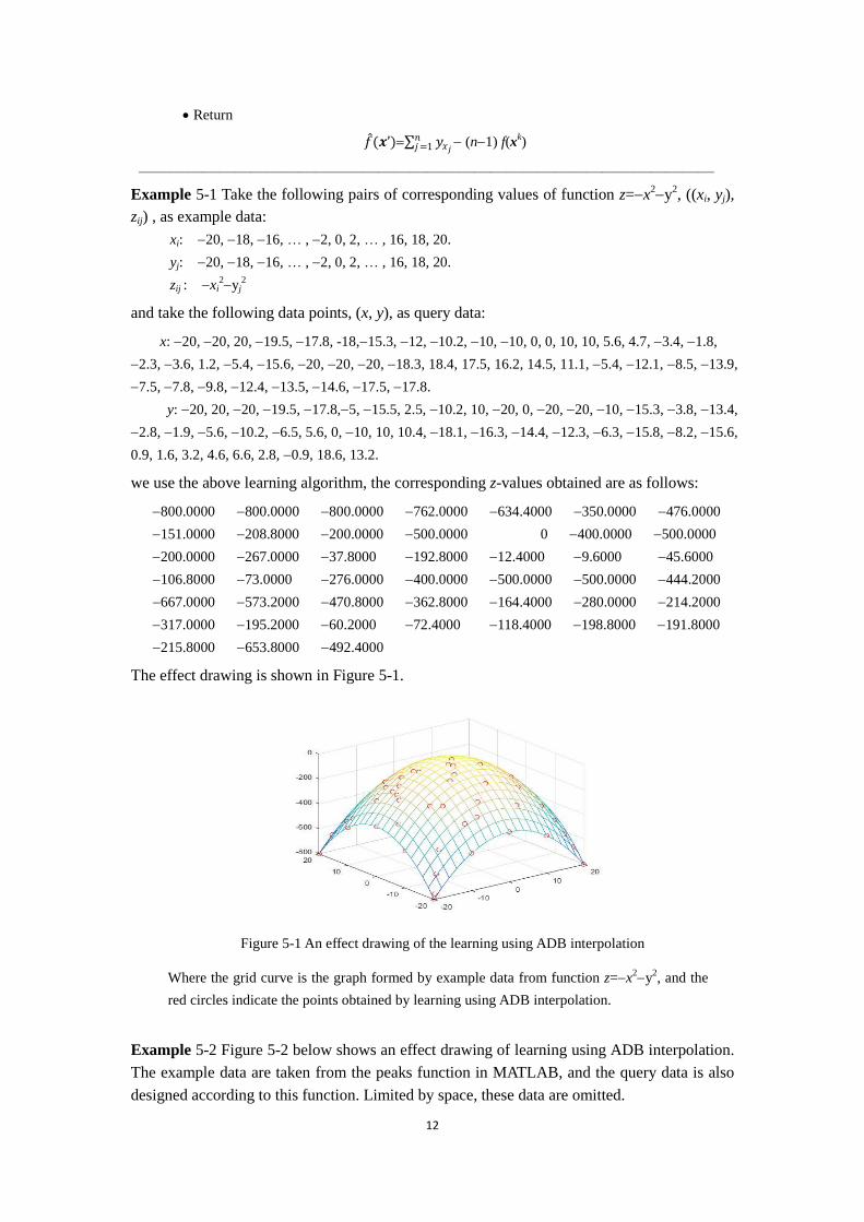
The effect drawing is shown in Figure 5-1.
Example 5-2 Figure 5-2 below shows an effect drawing of learning using ADB interpolation.
The example data are taken from the peaks function in MATLAB, and the query data is also
designed according to this function. Limited by space, these data are omitted.
Figure 5-1 An effect drawing of the learning using ADB interpolation
Where the grid curve is the graph formed by example data from function z=x2y
2, and the
red circles indicate the points obtained by learning using ADB interpolation.

13
As can be seen from the above, this instance-based learning using ADB interpolation has
the following characteristics:
The learning method takes data points (xl) of training examples ((x
l, f(x
l)) as centers to
set approximation regions and compute approximation-degrees.
ADB interpolation is a local interpolation, the training examples involved in
interpolation are related to the position of the currently queried data point x’ relative to its
nearest data point xk, the number of which is related to the dimension of the vector x,
n-dimensional x only involves 1+n training examples ((xk, f(x
k)) and (x
1, f(x
1)), (x
2, f(x
2)), … ,
(xn, f(x
n)) ). But since the point x’ is only approximate to the point x
k, the corresponding 𝑦𝑥𝑗
(j=1,…, n) are most affected by the example (xk, f(x
k)), and the final synthesized value 𝑓 (𝒙’)
is also most affected by (xk, f(x
k)).
If distributed storage and parallel processing (including parallel lookup and parallel
computation) are used, the time complexity of corresponding algorithm is independent of the
dimension of vector x, and its efficiency is almost equal to that of one-dimensional
interpolation at all time.
The interpolation formulas (including sum-times-difference formula) are derived
entirely by the mathematical method, so they have definite mathematical basis.
The sum-times-difference formula is actually a linear combination of coordinate
components of an interpolation point, and the denominators of the coefficients before each
coordinate component are separately the difference between the coordinate component and
the corresponding coordinate component of corresponding base point, that is, the distance
between the two, so, these coefficients happen to also have a function of the weight values.
Thus, viewed from the form, the sum-times-difference formula is a linear weighted regression
formula. That is to say, the sum-times-difference formula here coincides with the traditional
local weighted linear regression model. However, in local weighted linear regression, these
coefficients are determined by searching, i.e., learning, while in our ADB interpolation, these
coefficients are determined by looking up. The former is guided and constrained by error
Figure 5-2 An illustration of the effect of learning using ADB interpolation
Where the left is the functional graph formed by example data, and the right is the functional
graph obtained by learning using ADB interpolation.
(a) (b)

14
function (e.g. E=1
2 (𝑓 𝒙 − 𝑓 𝒙 )2𝒙∈𝑋1𝑋 ), and the latter by approximation-degree function
(e.g. 𝐴𝑥𝑖(𝑥)). In the sense of approximation-degree, the approximate value 𝑓 (𝒙’) of the
function obtained from the sum-times-difference formula is always the most accurate.
The accuracy of the returned approximate value 𝑓 (𝒙’) of a function is positively
related to the approximation-degree of x’ to xk.
Comparing the learning using ADB interpolation with the deep learning, the deep
learning is to approximate objective function with the strategy of deepening vertically[9]
, yet
the learning using ADB interpolation can approximate objective function with the strategy of
increasing density horizontally. So, the learning using ADB interpolation and the deep
learning can complement each other, and can even have an effect of “different approaches but
equal results” in the case of sufficient samples.
(2) A learning algorithm for classification problems
————————————————————————————————————
Put samples in sample set X={(𝒙𝑖 , 𝑓(𝒙𝑖))}𝑖=1𝑚 (x=(x1, x2 … , xn), f(x) is a class label )
into a corresponding data structure S in centralized or distributed manner; (as training
examples)
For the currently being queried x’=(x1’, x2’, … , xn’):
According to its coordinate components x1’, x2’, … , xn’ look up in S sequentially or
in parallel to determine a xk (k{1,2,…,m}) to which the approximation-degree of x’
is highest;
If such a xk is found, return
𝑓 (𝒙’) f(xk)
Else exit.
————————————————————————————————————
Example 5-3 Suppose that the data points of training examples of a classification problem
are shown as the black circles in Figure 5-3, and the small boxes surrounding them are their
respective strict approximation regions; and the white circles represent data points to be
classified. Using the learning algorithm that using ADB interpolation to classify these data
points, the classifying results are shown in the figure. As you can see, there are two queried
data points are respectively classified to two classes to which the corresponding training
example data points belong, because they are located respectively in the strict approximation
regions of the corresponding data points, while the two queried data points outside the small
boxes are not classified.
It can be seen that for classification problems, the learning using ADB interpolation has
the following advantages:
Although similar to the traditional 1-NN algorithm, the approximation regions in the
algorithm are aimed at the data points of training examples, and which are strict
approximation regions of square.
Since the approximation and approximation regions involved in the algorithm are strict
approximation and strict approximation regions, for classification problems, learning using
ADB interpolation avoids, from the source, the problem in traditional instance-based learning
(e.g. k-NN algorithm) that some datum objects with similar partial attributes are classified

15
into a class.
The classifying result of learning using ADB interpolation is unique, and there is no the
phenomenon like k-NN algorithm, that classifying result may change with the change of k’s
value.
6 Summary
In this paper, started from finding approximate value of a function, we introduced the measure
of approximation-degree between two numerical values, proposed the concepts of "strict
approximation" and "strict approximation region", then, derived the corresponding
one-dimensional interpolation methods and formulas, and then presented a calculation model
called "sum-times-difference formula" for high-dimensional interpolation, thus we developed
a new interpolation approach approximation-degree-based interpolation, i.e., ADB
interpolation. ADB interpolation was applied to the interpolation of actual functions with
satisfactory results. Viewed from principles and examples, the approach is of novel idea, and
it has the advantages of simple calculations (they are all arithmetic), stable accuracy
(benefitting from local interpolation and that the approximation-degrees are always not less
than 0.5); especially, the approach facilitates parallel processing, very suiting for
high-dimensional interpolation, and easy to be extended to the interpolation of vector valued
functions.
Applying ADB interpolation to instance-based learning, we obtained a new
instance-based learning method learning using ADB interpolation, and we also gave
several examples of the learning. Viewed from principles and examples, the learning method
is of unique technique (e.g., taking data points of training examples as centers to set
approximation regions that are also strict approximation regions and compute
approximation-degrees). Besides the advantages of ADB interpolation, the learning method
has also the advantages of definite mathematical basis, implicit distance weights, avoiding
misclassification (guaranteed by strict approximation), high efficiency (benefitting from
distributed storage and parallel processing), and wide range of applications (which can be
applied to the regression or classification problems, and can be used for large sample learning
or small sample even single sample learning), as well as being interpretable, etc. In principle,
this method is a kind of learning by analogy, which and the deep learning that belongs to
inductive learning can complement each other, and for some problems, the two can even have
Figure 5-3 An illustration of applying the learning using ADB interpolation to classification
x2
x3
x4
x1
x5
x1
x2
16
an effect of “different approaches but equal results” in big data and cloud computing
environment. Thus, the learning using ADB interpolation can also be regarded as a kind of
“wide learning” that is dual to deep learning.
References
[1] Tom M. Mitchell, Machine Learning, MecGraw-Hill Companies, Inc.1997, pp. 165178.
[2] Stuart Russell, Peter Norvig. Artificial Intelligence:A Modern Approach (Second Edition). London:
Pearson Education Limited, 2003, pp. 565568.
[3] Ethem Alpaydin, Introduction to Machine Learning (Third Edition), Massachusetts Institute of
Technology, 2014, pp. 107123.
[4] Stuart J. Russell, Peter Norvig. Artificial Intelligence:A Modern Approach (Third Edition). London:
Pearson Education Limited, 2016, pp. 737744.
[5] Shiyou Lian, Correspondence between Flexible Sets, and Flexible Linguistic Functions, in: Shiyou
Lian, Principles of Imprecise-Information Processing: A New Theoretical and Technological
System, Springer Nature, 2016, pp. 205228.
[6] Shiyou Lian, Approximate Evaluation of Flexible Linguistic Functions, in: Shiyou Lian, Principles
of Imprecise-Information Processing: A New Theoretical and Technological System, Springer
Nature, 2016, pp. 393417.
[7] Shiyou Lian. Principles of Imprecise-Information Processing: A New Theoretical and Technological
System, Springer Nature, 2016.
[8] Shiyou Lian, Multidimensional Flexible Concepts and Flexible Linguistic Values and Their
Mathematical Models, in: Shiyou Lian, Principles of Imprecise-Information Processing: A New
Theoretical and Technological System, Springer Nature, 2016, pp. 4579.
[9] Yoshua Bengio, Deep Learning, July 23, 2015, LxMLS 2015, Lisbon Machine Learning Summer
School, Lisbon Portugal, http://www.iro.umontreal.ca/~bengioy/talks/lisbon-mlss-19juillet2015.pdf