a study on the profit-based quality-productivity
TRANSCRIPT
A STUDY ON THE PROFIT-BASED QUALITY-PRODUCTIVITY
RELATIONSHIP MODEL AND ITS VERIFICATION
IN MANUFACTURING INDUSTRIES
by
WEN-RUEY LEE, B.E., M.S.E.
A DISSERTATION
IN
INDUSTRIAL ENGINEERING
Submitted to the Graduate Faculty of Texas Tech University in
Partial Fulfillment of the Requirements for
the Degree of
DOCTOR OF PHILOSOPHY
Approved
Accepted
May, 1997

ACKNOWLEDGMENTS AKS-B^I
l\oy ly ^ I would like to express my sincere gratitude to Drs. Mario G. Beruvides,
James L. Smith, Jerry D. Ramsey, Hong-Chao Zhang, and Paul H. Randolph for
serving on my dissertation committee and for the guidance they have given me. I also
sincerely thank Dr. William J. Conover for his sage counsel and provision of related
software to this work.
I am especially indebted to my advisor. Dr. Mario G. Beruvides, for his
valuable suggestions, and patient guidance throughout my Ph.D. study. To me. Dr.
Beruvides is not only an excellent advisor but also a dear friend. Without his help, I
would not be who I am now.
Many others have contributed to this work throughout the years. Their
support is gratefully acknowledged. Especially, I would like to thank Mr. Chien K.
Lin, Mr. Yi T. Lin, Mr. Chin Y. Wu, Mr. Min H. Liao, Mr. Ming T. Chen, and Mr.
Meng C. Lin who assisted this research with great zeal in the data collection in the
field study.
I am grateful to my loving wife, Huei-Jen Homg, who gave me full support
during the days of studying at Texas Tech University. Finally, I would like to
dedicate this work to my father in commemoration of his passing away after my
dissertation defense.
11
TABLE OF CONTENTS
ACKNOWLEDGMENTS ii
LIST OF TABLES xii
LIST OF FIGURES xiv
CHAPTER
I. INTRODUCTION 1
1.1 Research Problem Statement 4
1.2 Scope of This Research 5
1.2.1 Research Question 6
1.2.2 Research Purpose 6
1.2.3 Research Objective 7
1.2.4 General Hypotheses 7
1.3 Limitations and Assumptions 8
1.3.1 Limitations 8
1.3.2 Assumptions 9
1.4 Relevance 9
1.4.1 Need for This Research 10
1.4.1.1 Theoretical Research Needs 10
1.4.1.2 Practical Research Needs 11
1.4.2 Benefits of This Research 11 1.5 Expected Results 12
111
2. LITERATURE REVIEW 13
2.1 Background 13
2.1.1 History 13
2.1.1.1 History of Quality 14
2.1.1.2 History of Productivity 16
2.1.1.3 Review of the Relationship between Quality and Profit 19
2.1.1.4 Review of the Relationship between Productivity and Profit 25
2.1.1.5 Review of the Relationship between Quality and Productivity 29
2.1.2 Definitions 36
2.1.2.1 Definitions of Productivity 37
2.1.2.2 Definitions of Quality 43
2.1.2.3 Definitions of Profitability and Profit 49
2.2 Current Profit-Based Quality, Productivity Models 53
2.2.1 Quality-Cost Model 53
2.2.1.1 Optimum Quality Cost Model 54
2.2.1.2 Dawes' Quality Cost Model 55
2.2.1.3 Poor-Quality Cost (PQC) Model 57
2.2.1.4 Taguchi's Quality Loss Function Model 59
2.2.2 Productivity-Profit Model 60
2.2.2.1 Adam-Hershauer-Ruch's Productivity-Profit Relationship Model 60
2.2.2.2 Papadimitriou's Profit Decomposition Model (PDM) 61
2.2.2.3 Sumanth's Productivity-Profit Relationship Model 64
iv
2.2.2.4 APC's Productivity-Profit Relationship Model 67
2.2.2.5 Miller's Productivity-Profit Relationship Model 67
2.2.2.6 Miller's Productivity-ROI Relationship Model 69
2.2.3 Quality-Productivity Relationship Models 71
2.2.3.1 Adam-Hershauer-Ruch Model 72
2.2.3.2 Deming's Model 73
2.2.3.3 Edosomwan's Model 73
2.2.3.4 Thor's Model 78
2.2.3.5 Sumanth's Quality-Profit-Productivity Relationship Model 80
2.3 Deficiencies and Limitations of Current Models 84
2.3.1 Deficiencies and Limitations of Quality-Profit Model 84
2.3.2 Deficiencies and Limitations of Productivity-Profit Model 87
2.3.3 Deficiencies and Limitations of Quality-Productivity Model 90
2.4 Research Agenda 95
2.4.1 Definitions of This Research 95
2.4.1.1 Definition of Quality 95
2.4.1.2 Definition of Productivity 96
2.4.1.3 Definition of Profit 98
2.4.1.4 Definition of Cost 98
2.4.2 Conceptual and Mathematical Models 100
2.4.2.1 Relationships among Quality, Price, Revenue, Volume Sold, and Costs 100
V
2.4.2.1.1 Price-Volume-Quality Relationship 100
2.4.2.1.2 Revenue-Quality Relationship 100
2.4.2.1.3 Cost-Volume-Quality Relationship 102
2.4.2.1.4 Cost-Quality Relationship 102
2.4.2.2 Quality-Profit Model 103
2.4.2.3 Productivity-Profit Model 105
2.4.2.4 Quality-Productivity Model 106
2.4.2.5 Conceptual Model of Linking Productivity and Quality in Confirmatory Study 108
2.4.2.6 The Comparison between the Proposed Model of This Research and Sumanth and Wardhanas' Model 109
2.4.2.7 Advantages of Relating Quality-Profit and Quality-Productivity
Models Based on Ranks 113
2.4.2.8 Contributions of This Research 114
3. RESEARCH METHODOLOGY 116
3.1 Research Process 116
3.2 Research Design 118
3.2.1 Type of Research 119
3.2.2 Research Focus 119
3.2.3 Research Hypotheses 120
3.2.4 Research Environment 123
3.2.4.1 ABC Company 123
3.2.4.2 XYZ Company 125
vi
3.2.5 Research Method 127
3.2.6 Research Instrument 127
3.2.7 Measurement of Costs and Profit 127
3.2.7.1 Measurement of Costs 129
3.2.7.2 Measurement of Profit 129
3.2.8 Test Plans of This Research 130
3.2.9 Specific Models Establishment 120
3.2.10 Unit of Analysis 135
3.2.10.1 ABC Company 135
3.2.10.2 XYZ Company 136
3.3 The Collection and Treatment of Data 136
3.3.1 Data Collection 137
3.3.2 Treatment of Data 137
3.4 Methodological Issues 140
3.4.1 Reliability 140
3.4.2 Validity 142
3.4.3 Replicability 144
3.4.4 Bias 145
3.4.5 Representativeness 147
3.5 Research Constraints 147
4. FIELD STUDY RESULTS, ANALYSIS, AND DISCUSSION 149
vu
4.1 Introduction 151
4.1.1 Company Contacts 151
4.1.2 Operation Definition 152
4.1.3 Primary Data Collected 154
4.1.4 Secondary Data Collected 154
4.2 Results of Collected Data 156
4.2.1 Production Cost Data 156
4.2.2 Revenue Data 158
4.2.3 Profit Data 160
4.2.4 Quality Data 162
4.2.5 Productivity Data 164
4.3 Data Analysis 166
4.3.1 Confirmatory Analysis 166
4.3.1.1 Method of Analysis 167
4.3.1.2 Quality-Profit Analysis 169
4.3.1.2.1 Spearman's Rho Test 169
4.3.1.2.2 Normality Test 171
4.3.1.2.3 Estimation of Confidence Interval of Correlation Coefficient 171
4.3.1.3 Productivity-Profit Analysis 172
4.3.1.3.1 Spearman's Rho Test 172
4.3.1.3.2 Normality Test 174
4.3.1.3.3 Estimation of Confidence Interval of Correlation Coefficient 174
viii
4.3.1.4 Quality-Productivity Analysis 175
4.3.1.4.1 Spearman's Rho Test 175
4.3.1.4.2 Normality Test 176
4.3.1.4.3 Estimation of Confidence Interval of Correlation Coefficient 177
4.3.2 Model Analysis 178
4.3.2.1 Method of Analysis 178
4.3.2.2 Quality-Profit Relationship Model Analysis 180
4.3.2.2.1 Specific Linear Regression Models 180
4.3.2.2.2 Residual Plots 181
4.3.2.2.2.1 Plots: Residuals Against r(Q) ~ Check the Linearity and Constant Variance 181
4.3.2.2.2.2 Plots: Residuals Against Time ~ Check the Nonindependence of Error Terms 184
4.3.2.2.2.3 Plots: Residuals Against Expected Values ~ Check the Normality of Error Terms 188
4.3.2.3 Productivity-Profit Relationship Model Analysis 190
4.3.2.4 Quality-Productivity Relationship Model Analysis 191
4.3.2.4.1 Specific Linear Regression Models 191
4.3.2.4.2 Residual Plots 192
4.3.2.4.2.1 Plots: Residuals Against r(Q) ~ Check the Linearity and Constant Variance 192
4.3.2.4.2.2 Plots: Residuals Against Time ~ Check the nonindependence of Error Terms 194
4.3.2.4.2.3 Plots: Residuals Against Expected Values ~ Check the Normality of Error Terms 197
IX
4.4 General Discussion 199
4.4.1 Discussion of Quality-Profit Relationship 199
4.4.2 Discussion of Productivity-Profit Relationship 200
4.4.3 Discussion of Quality-Productivity Relationship 202
4.4.4 Discussion of Data 204
5. CONCLUSIONS AND RECOMMENDATIONS 205
5.1 Summary 205
5.2 Further Discussion and Implications 208
5.2.1 Further Discussion 208
5.2.2 Implications 209
5.3 Conclusions 211
5.4 Recommendations 212
5.4.1 Theoretical Recommendations 212
5.4.2 Practical Recommendations 213
BIBLIOGRAPHY 214
APPENDIX
A: MATHEMATICAL MODELS DEVELOPMENT 234
B: QUALITY INSPECTION POINTS IN ABC AND XYZ COMPANIES 243
C. TABLE FOR THE SPEARMAN'S RHO TEST 246
D: RESULTS OF THE LILLEEFORS NORMALITY TESTS 248
E: A PROOF FOR THE RELATIONSHIP BETWEEN SLOPE OF A REGRESSION LINE BASED ON RANKS AND ITS CORRELATION 261
X
F: THE DURBIN-WATSON TEST PROCEDURE AND ITS TABLE 264
G: PREDICTED VALUES OF SPECIFIC MODELS OF QUALITY-PROFIT RELATIONSHIP 267
H: PREDICTED VALUES OF SPECIFIC MODELS OF QUALITY-PRODUCTIVITY RELATIONSHIP 271
XI
LIST OF TABLES
2.1 Definitions ofproductivity in the open literature 38
2.2 Definitions of quality in the open literature 44
2.3 Definitions of profitability and profit in the open literature 50
2.4 Comparison of QPR Values When Unit Reject Processing Cost Significantly Decreases 92
4.1 Definitions of Quality and Productivity in the ABC and XYZ Companies 153
4.2 Production Cost Data of Gingham in the ABC Company 157
4.3 Production Cost Data of Piece-dyed Fabric in the ABC Company 157
4.4 Production Cost Data of Token Ring in the XYZ Company 157
4.5 Production Cost Data of PNP Ethernet Combo in the XYZ Company 158
4.6 Revenue Data of Gingham in the ABC Company 158
4.7 Revenue Data of Piece-dyed Fabric in the ABC Company 159
4.8 Revenue Data of Token Ring in the XYZ Company 159
4.9 Revenue Data of PNP Ethernet Combo in the XYZ Company 159
4.10 Profit Data of Gingham in the ABC Company 160
4.11 Profit Data of Piece-dyed Fabric in the ABC Company 160
4.12 Profit Data of Token Ring in the XYZ Company 161
4.13 Profit Data of PNP Ethernet Combo in the XYZ Company 162
4.14 Quality Conformance Level of Gingham in the ABC Company 163
4.15 Quality Conformance Level of Piece-dyed Fabric in the ABC Company 163
Xll
4.16 Quality Conformance Level of Token Ring in the XYZ Company 163
4.17 Quality Conformance Level of PNP Ethernet Combo in the XYZ Company.. 164
4.18 Productivity Data of Gingham in the ABC Company 164
4.19 Productivity Data of Piece-dyed Fabric in the ABC Company 165
4.20 Productivity Data of Token Ring in the XYZ Company 165
4.21 Productivity Data of PNP Ethernet Combo in the XYZ Company 165
4.22 Summary of Spearman's Rho Test Results for Quality-Profit Relationship 170
4.23 Summary of Spearman's Rho Test Results for Productivity-Profit Relationship 173
4.24 Summary of Spearman's Rho Test Results for Quality-Productivity Relationship 176
4.25 Summary of the Estimated Linear Regression Models for Quality-Profit Relationship 181
4.26 The Durbin-Watson Test Results for the Quality-Profit Relationship of PNP and Token Ring Cases 187
4.27 Summary of the Estimated Linear Regression Models for Quality-Productivity Relationship 191
4.28 The Durbin-Watson Test Results for the Quality-Productivity Relationship of PNP and Token Ring Cases 196
5.1 Summary of Mathematical Models of This Research 207
B.l Quality Inspection Points in ABC and XYZ Companies 244
C. 1 Quantiles of the Spearman Test Statistic 247
F.l Durbin-Watson Test Bounds 266
G.l Predicted Values of Specific Models of Quality-Profit Relationship 268
H. 1 Predicted Values of Specific Models of Quality-Productivity Relationship 272
xiu
LIST OF FIGURES
2.1 Model for Optimum Quality Costs 54
2.2 New model for Optimum Quality Costs 55
2.3 Dawes'Quality-Cost Model 56
2.4 Effect of varying controllable PQC 58
2.5 Taguchi's Quality Loss Function 59
2.6 The Relationship between Profits and Input Costs 66
2.7 Chain Reaction Related to Quality and Productivity 73
2.8 A Framework for Understanding the Connection and Relationship between Productivity and Quality 74
2.9 Components of the PQMM 77
2.10 Process Quality and Productivity Are Essentially the Same 78
2.11 A Complete Productivity and Quality Measurement System 79
2.12 Costs of Non Quality and Quality Efforts as a Function of Quality of Conformance 82
2.13 The Relationships between Quality of Conformance, Profit, and Total Productivity 83
2.14 Cost-Profit Relationship 85
2.15 Price-Volume-Quality Relationship lOl
2.16 Revenue-Quality Relationship 101
2.17 Production Cost-Volume-Quality Relationship 102
2.18 Production Cost-Quality Relationship 103
XIV
2.19 Quality-Profit Relationship 105
2.20 Productivity-Profit Relationship 106
2.21 Quality-Productivity Relationship 107
2.22 Conceptual Model of Linking Quality and Productivity 109
3.1 Research Process of This Study 117
3.2 Main Hypotheses of This Research 121
3.3 Sub-Hypotheses of This Research 122
3.4 The Production Process of Gingham in the ABC Company 124
3.5 The Production Process of PNP Ethernet Combo in XYZ Company 126
3.6 Research Method in the Field Study 128
3.7 Test Plan for Quality-Profit Relationship 131
3.8 Test Plan for Productivity-Profit Relationship 132
3.9 Test Plan for Quality-Productivity Relationship 133
3.10 Data Collection Form 138
4.1 Research Sequence of Chapter 4 150
4.2 Residual Plots: Residuals Against Ranks of Quality 182
4.3 Residual Time Plots: Residuals Against Time Series 185
4.4 Residual Plots: Residuals Against Expected Value 189
4.5 Residual Plots: Residuals Against Ranks of Quality 192
4.6 Residual Time Plots: Residuals Against Time Series 194
4.7 Residual Plots: Residuals Against Expected Value 197
XV
D. I Normality Test for Quality-Profit Data of Gingham (Factory A, ABC Company) 249
D.2 Normality Test for Quality-Profit Data of Gingham (Factory B, ABC Company) 249
D.3 Normality Test for Quality-Profit Data of Gingham (Factory C, ABC Company) 250
D.4 Normality Test for Quality-Profit Data of Piece-dyed Fabric (Factory A, ABC Company) 250
D.5 Normality Test for Quality-Profit Data of Piece-dyed Fabric (Factory B, ABC Company) 251
D.6 Normality Test for Quality-Profit Data of Piece-dyed Fabric (Factory C, ABC Company) 251
D.7 Normality Test for Quality-Profit Data of PNP Ethernet Combo 252
D.8 Normality Test for Quality-Profit Data of Token Ring 252
D.9 Normality Test for Productivity-Profit Data of Gingham (Factory A, ABC Company) 253
D. 10 Normality Test for Productivity-Profit Data of Gingham (Factory B, ABC Company) 253
D. 11 Normality Test for Productivity-Profit Data of Gingham (Factory C, ABC Company) 254
D. 12 Normality Test for Productivity-Profit Data of Piece-dyed Fabric (Factory A, ABC Company) 254
D.13 Normality Test for Productivity-Profit Data of Piece-dyed Fabric (Factory B, ABC Company) 255
D. 14 Normality Test for Productivity-Profit Data of Piece-dyed Fabric (Factory C, ABC Company) 255
D. 15 Normality Test for Productivity-Profit Data of PNP Ethernet Combo 256
D. 16 Normality Test for Productivity-Profit Data of Token Ring 256
XVI
D. 17 Normality Test for Quality-Productivity Data of Gingham (Factory A, ABC Company) 257
D. 18 Normality Test for Quality-Productivity Data of Gingham (Factory B, ABC Company) 257
D. 19 Normality Test for Quality-Productivity Data of Gingham (Factory C, ABC Company) 258
D.20 Normality Test for Quality-Productivity Data of Piece-dyed Fabric (Factory A, ABC Company) 258
D.21 Normality Test for Quality-Productivity Data of Piece-dyed Fabric (Factory B, ABC Company) 259
D.22 Normality Test for Quality-Productivity Data of Piece-dyed Fabric (Factory
C, ABC Company) 259
D.23 Normality Test for Quality-Productivity Data of PNP Ethernet Combo 260
D.24 Normality Test for Quality-Productivity Data of Token Ring 260
xvii
CHAPTER I
INTRODUCTION
For years quality and productivity have been regarded as two important
indexes of company performance. Many companies hope to pursue high quality and
high productivity at the same time. However, in most cases, these two variables are
not linked together in the production system mainly because of the variety of their
definitions (Human Resources Productivity, 1983; Garvin, 1988; Belcher, 1987;
Hoffherr & Moran & Nadler, 1994; Smith, 1990). Additionally, these two variables
are not taken into account together because: (1) the objectives of quality management
and productivity management are viewed as contradictory,^ (2) the definitions of
quality and productivity are difficult to define, (3) the affecting factors on quality or
productivity are too numerous, (4) seemingly, quality and profit have no direct
connection,^ and (5) many companies believe that they have distinct characteristics
which may not be subject to any model.
' Deming (1986), Belcher (1987), Darts (1990), Hart and Hart (1989), Kaydos (1991), and Omachonu and Ross (1994) also have noted this misconception in their research.
^ Pirsig (1974) believes quality cannot be defined. McNealy (1993) states that quality is as hard as "art" to define. Mohanty and Yadav (1994) also claim that quality is a difficult concept to define. Deming (1986) maintains that quality is defined by management. Kendrick (1984) asserts that productivity cannot be measured directly. Yet others, such as Smith (1986), Kaydos (1991), Price (1990), regard quality and productivity as the same thing.
^ Sumanth and Wardhana (1993) point that some companies do not believe "quality and profit go hand in hand," (p. 463)
The first reason, stated above, was especially prevalent in the past. Deming
(1986) asserts that this erroneous concept of quality and productivity management
contradiction is common in American industries; therefore, he firmly asserted that
improving quality will result in improved productivity. He believed the relationship
between quality and productivity is strongly positive. However, he interpreted this
relationship by reasoning, that is, Deming presented no mathematical model to
backup his assertion. Managers believe his assertion is correct because the logic is
reasonable.
The second reason that quality and productivity are difficult to define, lies in
the debatable definitions. So far the well-known definitions of quality are too
abstract to relate to productivity. On the other hand, productivity has different levels
(or units of analysis) and types.' Each level or type ofproductivity has different units
of measure. The type or unit of measure for productivity which should be used to
relate to quality is debatable.
The third reason, that the affecting factors on quality or productivity are too
numerous, illustrates the difficulties of relating quality and productivity. Generally,
the current quality-productivity relationship models can be classified into two
categories: qualitative models and quantitative models. The qualitative models
outnumber the quantitative models because the latter need measurable variables. A
'* Sumanth (1979) deals with productivity at four levels: International, National, Industry, Company. Sumanth (1994) classifies productivity into three types: Total Productivity, Total Factor Productivity, and Partial Productivity. Kendrick (1984) deals with productivity at another four levels: National, Industrial, Company, and Personal.
qualitative model is easier to understand, but has less applicability compared with a
quantitative model. However, because many factors are not easy to measure,
quantitative models have limitations in application. Therefore, companies may not
believe it is practical to link quality and productivity.
The fourth reason, that quality and profit have no direct connection, illustrates
that current models cannot reflect the impact on profit. Profit is the main concern of
management, ff a quality-productivity model cannot estimate the impact on profit, it
loses its attractiveness to the management. However, because quality is an abstract
concept, it is hard to directly link quality and profit together. Although productivity
can be measured in terms of profit, it is not common to quantitatively relate quality to
profit. Therefore, a quality-productivity model without profit as a base may not be
attractive to industries.
The last reason, that each company believes it has its own characteristics
which may not be subject to any model, illustrates their perception that their
production features are different from others. They believe that a model may be
applicable to others, but not to them. Each company has its own production features;
however, a generic model can be tailored to the user's own purpose. Most models
found in open literature are not originally developed for a specific company. Hence,
the notion that it is impractical to link quality and productivity for use is incorrect.
These five reasons leave the following questions unanswered: High quality
and high productivity are all pursued by companies, but how can they be related to
each other? Is this potential relationship model meaningful for companies? How can
the relationship be applied in practice? This study will answer all these questions.
This research focuses on the profit-based quality-productivity relationship
model and its verification in manufacturing industries. In this chapter, the problem
statement is presented in section 1.1. The scope of this research, including the
research question, purpose and objective, are addressed in section 1.2. The
limitations and assumptions of this research are presented in section 1.3. In section
1.4, needs and benefits of this research are explained. Finally, section 1.5 presents
the expected results.
1.1 Research Problem Statement
Quality and productivity are two measures of interest in most every company.
Their relationship is also a concern of management. From the open literature, it is
understood that productivity will increase as product quality increases (Shetty &
Buehler, 1985; Hayes, 1985; Deming, 1986; Hart & Hart, 1989; Darts, 1990; Kaydos,
1991; Tribus, 1992; Barrett, 1994; Omachonu & Ross, 1994). However, fewer
quality-productivity relationship models are expressed in a mathematical way. A
mathematical model of the quality-productivity relationship provides more clear
information for parameter control than does a descriptive model. Therefore, an
appropriate mathematical model relating quality and productivity is sought to meet
the needs of management.

Since multiple units of measure are used in quality as well as productivity
measures, a common measurement unit must be set in order to relate quality and
productivity. Perhaps a better common unit of measure in this quality-productivity
relationship is profit, since profit is most attractive to management. Hence, a study on
the profit-based quality-productivity relationship model is conducted in this research.
Finally, the applicability of the developed quality-productivity relationship
model must be discussed. A study on the verification of this proposed model in
Taiwan's manufacturing industries is surveyed. Taiwan's manufacturing industries
are chosen for the follovWng reasons: (1) Taiwan is a typical Newly Industrialized
State (NIS). The government adopts an export-oriented trading policy. This policy
encourages all enterprises to emphasize quality and productivity, (2) Many managers
in Taiwan's manufacturing industries possess common knowledge of quality control
and productivity management. This is especially helpful in communication when
conducting this research, (3) Information on Taiwan's manufacturing industries is
readily available for this research.
1.2 Scope of This Research
This section addresses the research question in which this study is interested.
The research purpose and objective are also included in this section to help direct the
efforts of this research.

1.2.1 Research Question
The main questions this work will address are as follows:
1. What is the quality-productivity relationship model based on profit?
2. Is the profit-based quality-productivity relationship model applicable in
manufacturing environment?
To answer the two main questions, it is necessary to understand further:
a. What is the quality-profit relationship?
b. What is the productivity-profit relationship?
c. How many quality-productivity relationship models are currently
available? Are they generic or specific? Do they need to be revised or
modified for this research?
1.2.2 Research Purpose
This research will attempt to provide an applicable profit-based quality-
productivity relationship model for manufacturing industries. This model will
convince the management of that quality and productivity are positively related, and
the enhancement of either quality or productivity will increase profit. An additional
purpose of this research is to show whether the developed quality-productivity
relationship model is applicable to an individual company. It is expected that the
developed model is not only theoretically sound, but also may be practically used by
companies in the real world.
1.2.3 Research Objective
This research has two main objectives: (1) develop a mathematical quality-
productivity relationship model based on profit, and (2) Investigate the applicability
of this model in the manufacturing industries.
In achieving these objectives, the following secondary objectives are included:
1. To review the existing models related to the quality-productivity
relationship.
2. To explore the relationship between quality and profit.
3. To explore the relationship between productivity and profit.
4. To conduct an empirical study in Taiwan in order to confirm the
developed model.
1.2.4 General Hypotheses
The general hypotheses regarding this research are:
1. Quality and profit are related, and a model may illustrate the relationship
between these variables.
2. Productivity and profit are positively related, and there is a model to relate
these two variables.
3. Quality and productivity are related, and a model may illustrate the
relationship between these variables.
1.3 Limitations and Assumptions
In this research, some determination of the limitations and assumptions is
required. These limitations and assumptions are helpftil in focusing this research. If
the model proposed in this research is tailored for a specific purpose, the limitations
or assumptions will possibly change.
1.3.1 Limitations
The limitations of this research are:
1. This research deals only with manufacturing companies. Service
organizations will not be included in the scope of this research.
2. The intangible factors of quality and productivity are not discussed in this
research.
3. The relationship between quality and productivity is linked based on profit.
4. The productivity measure (unit of analysis) used in this research is limited
to the company level. The productivity measures of national, industrial,
and individual levels are not considered in this study.
5. The productivity type used in relating productivity to quality is restricted to
the Total Productivity Model.
6. The study on the applicability of proposed model is conducted in Taiwan's
manufacturing organizations.
8
7 This research considers all issues within this research from an industrial
engineering perspective. Implications concerning other disciplines are not
addressed in depth.
1.3.2 Assumptions
The assumptions of this research are:
1. The manufacturing company is a profit-oriented company.
2. The company has the intention and capability of improving its quality and
productivity.
3. Quality can be linked wdth profit.
4. Productivity can be measured in terms of profit.
5. In general, the issues considered are applicable to manufacturing
companies.
6. Except where specified, all terms used in this research reflect the common
usage as found in the quality and productivity literature.
1.4 Relevance
This section describes the needs and benefits of this research. The needs of
this research provide the motive required for carrying out the research. Benefits of
this research are followed by the results of this study.
1.4.1 Need for This Research
This research deals with the theoretical relationships between quality,
productivity, and profit. A confirmatory study on the theoretical model is also
conducted to verify model's applicability. The specific theoretical and practical
research needs will be discussed in the following two subsections (1.4.1.1 and
1.4.1.2) respectively.
1.4.11 Theoretical Research Needs
Managers seek to improve quality by every possible means. They all
understand the importance of quality. However, the problem of how profit is affected
by quality is not easy to measure. In general, the relationship between quality and
profit is easier to explain in the descriptive approach; however, it lacks precision.
Perhaps a better way to realize how the quality level affects profit is to establish a
mathematical relationship model between these two variables. Through this
mathematical model, the optimal quality level in which the profit is maximum can be
identified.
The needs for research on the relationship between productivity and profit are
identical to those for quality and profit. The basic definition ofproductivity is a ratio
of output to input; therefore, if the output is measured in tenns of profit, it is easier to
quantitatively estimate the relationship between productivity and profit. However, it
10
is not easy to measure the relationship between productivity and profit without a
definite model. This research intends to determine such a mathematical model.
In addition, because productivity is strongly affected by quality, managers are
interested in their relationship. By establishing a Quality-Productivity relationship
model based on profit, it would help the managers and researchers realize more
firmly that profit can be increased by enhancing quality or productivity.
1.4.1.2 Practical Research Needs
This research is also interested in understanding the applicability of the
proposed model in manufacturing companies. Any model will undoubtedly be
accepted if it can be proved or confirmed. In general, management in industry is
more interested in the model's applicability than in the model's theory. Taiwan, as a
newly industrialized nation, has the desire to practically understand the relationships
between quality, productivity, and profit. This need is also a driving force of this
study.
1.4.2 Benefits of This Research
The benefits of this research are as follows:
1. Present an updated literature review on the quality-profit, productivity-
profit, and quality-productivity relationships.
11
2. Determine the relationship between quality and productivity from the profit
point of view.
3. Develop a relationship model of the quality and productivity that can be
analyzed and evaluated for the purpose of management.
4. Present a theoretical, quantitative research approach for measuring the
relationship between quality and productivity.
5. Confirm the proposed relationship model of quality and productivity
through field study.
1.5 Expected Results
This research should result in the following: (1) A mathematical model of the
quality-productivity relationship is to be set up fi-om the profit viewpoint. (2) The
applicability of the proposed model to manufacturing companies could be
investigated and verified. (3) The established specific model could be used as a
predictor for manufacturers. In addition to these three results, all of the relationship
models related to quality-profit, productivity-profit, and quality-productivity are to be
examined, analyzed, and classified through the literature review. Conclusions and
recommendations related to the findings of this research are also to be provided.
12
CHAPTER 2
LITERATURE REVIEW
2.1 Background
The quality-productivity relationship is linked by the measures of quality and
productivity. Because of the variety of quality and productivity measures, it is
necessary to base these two variables on a common unit of measure. Profit is
selected as this base because it relates to both quality and productivity. Besides,
profit is the most critical issue for management. In addition, to understand the basic
definitions and history of quality and productivity, it is also necessary to review the
relationships between quality, productivity, and profit. Therefore, in this section, the
history of quality and productivity are first briefly introduced. The relationships
between quality, profit, and productivity found in the open literature are then
presented. Various definitions of quality, productivity, and profitability are also
examined in this section.
2.1.1 History
History provides experiences and learning to deal with the future. It is helpful
to examine the history of quality and productivity before exploring the relationship
between the two variables. In addition to examining the history of quality and
productivity, these subsections illustrate the relationships between quality and profit.
13

productivity and profit, and quality and productivity. In order to more thoroughly
understand the quality-productivity relationship, review of this relationship is not
limited to profit-based.
2.1.1.1 History of Oualitv
The concept of quality has existed for a long time. According to Duncan
(1974), "Quality control is as old as industry itself (p. 1). Shewhart (1939) points out
more definitely that the inspection standard of a "go" tolerance limit appeared in
1840. About 30 years later, the improved concept of "go, no-go" tolerance limits
was developed. However, the management of quality, regarded as a professional
task, can be traced back to F. W. Taylor (1911). Known as the father of scientific
management, Taylor was the first to regard management and production as different
functions. In 1931, W. A. Shewhart (1931) introduced statistical quality control in
his book "Economic Control of Quality of Manufactured Product." In 1941, W. E.
Deming began to teach quality-control techniques in the U. S. War Department. He
later taught statistical quality control in Japan in 1950. To thank Deming for his
contribution, the Japanese established the Deming Prize in 1951. Another master in
quality control, J. M. Juran also gave seminars to the Japanese beginning in 1954.
^ In his book "The principles of scientific management," Taylor presented four principles for management. The fourth was "an almost equal division of the work and the responsibility between the management and the workmen," (p. 37). He indicated that nearly one-half of the production problem was up to the management. Therefore, he asserted that management was a professional task which should be separated fi-om the worker's job. According to Taylor's assertion, the management of quality should also be viewed as an independent function fi-om the worker's job.
14
This was "a turning point m emphasizing quality control for management" (Hosotani,
1992, p. 4).
It was not until the introduction of the concept of reliability that quality was
seldom measured relating to a product's life-time. Reliability engineering was
originated and conducted by the Advisory Group on Reliability of Electronic
Equipment (AGREE), formed in 1952, for studying and analyzing the failures of
electronic military equipment. The 1957 AGREE report formally defined the term
reliability and "formed the basis for modem methods and procedures" (Evans &
Lindsay, 1989, p. 255). In 1961, Martin Company developed the Zero Defects
Program and achieved zero defects in the American Army's Pershing missile system.
This Zero Defects concept was later introduced by J. F. Halpin, Director of Quality of
the Martin Company, in 1966. In the year of 1961, A. V. Feigenbaum first presented
the concept of Total Quality Control. K. Ishikawa introduced Quality Control Circles
in the following year. Mitsubishi's Kobe Shipyard in Japan first used Quality
Function Deployment (QFD) in 1972. The QFD technique was introduced to the U.
S. in 1983 by Professor Y. Akao of the University of Tamagawa. G. Taguchi, a
Japanese engineer, introduced a new approach in the early 1980s. His approach,
which later became known as the Taguchi Method, was used to design products and
reduce loss through what he termed the "Loss Function."
People are a very important factor to the quality. Research and
implementation related to the quality of work life (QWL) began to be emphasized.
15
According to Riggs and Felix (1983), the development of QWL can be traced to the
eariy 1970s. However, "Major efforts to make QWL an emerging fact in the
employees' work life have been under way since the 1980 National Memorandum of
Understanding was issued" (Shetty & Buehler, 1985, p. 135). Because of the risk
assumption, Shingo (1986) believes that traditional statistical methods cannot achieve
the zero defects level. In order to prevent and eliminate all possible defects, he then
proposed a mistake-proof system, called the poka-yoke system, and a source
inspection system. In 1987, the International Organization for Standardization (ISO)
published the ISO 9000 series to serve as the international standards of quality.
These standards were revised in 1994, and gradually have became more prevalent
since their adoption by many countries, especially the European Community nations.
The ISO 9000 series has become the supreme standards governing quality aspects.
Since the quality-productivity relationship is the key issue of this research, it
is also essential to understand the history ofproductivity. We will make a brief
introduction to its history in the following.
2.1.1.2 Historv of Productivity
According to Sumanth (1994), "probably, the first time the word 'productivity'
was mentioned was in an article by Quesnay in the year 1766" (p. 3). A more
detailed review ofproductivity is made by Kendrick (1977). In his book
Understanding Productivity, Kendrick mentioned that "the early estimates of
16
productivity were in terms of output per unit of labor input," (p. 19). This concept
was used by the eariy economists (e.g., Adam Smith in 1776) in the labor theory of
production and value (Kendrick, 1977). Kendrick recounted that in the latter
nineteenth century, Alfred Marshall advocated that man-made capital goods, labor,
and land were the basic factors of production. Marshall's recognition of the basic
factors of production became "the basis for the concepts of production function and
productivity" (Kendrick, 1977, p. 20).
The first estimates ofproductivity, in terms of output-per-hour, were
presented by the United States Bureau of Labor in the mid-1880s (Kendrick, 1977).
C. D. Wright, the first commissioner of labor in the U.S., published a report called
"Hand and Machine Labor," in 1898. According to Adam and Dogramaci (1981),
Wright's report, which studied company productivity and costs, is a remarkable
landmark in the history ofproductivity. Sumanth (1979) pointed out that probably the
first productivity index, a ratio of output to the number of wage earners, was
presented by F. C. Mills in 1899. Taylor (1911) in his renowned book The Principles
of Scientific Management, provided some examples for describing how the increase
in human productivity can be reached by applying the principles and methods of
scientific management. In addition, his work measurement is an effective tool for
improving labor productivity.
After the Great Depression of the 1930s, productivity estimates and analyses
were revived (Kendrick, 1977). During this period, the Bureau of the Census "began
17
publication of industry summaries on value added per man-hour" (Adam &
Dogramaci, 1981, p. 13). Since 1940, the Bureau of Labor Statistics (BLS)
investigated productivity performance in certain industries and published the first
regular government estimates ofproductivity. Today the BLS still "is the major
source of industrially based data on labor productivity" (Smith, 1990, p. xiii). The
initial development of the total factor productivity approach began after World War
II. According to Kendrick, productivity studies in the U. S. and abroad interacted
with the movement in many countries, beginning about 1950. The European
Productivity Agency, which became known as the European Association of National
Productivity Centers, was set up after 1952 to integrate the activities of the
international centers (Kendrick, 1977). Japan began its productivity movement in
1953. Two years later, the Japan Productivity Center began operation. The Asian
Productivity Organization, which is located in Tokyo, was established from the Japan
Productivity Center in 1961. No productivity agency was set up in the U. S. before
1970.
Due to "the failure to tax-finance the Vietnam escalation" and "the energy-
price revolution," inflation was actuated firom the mid-1960s to the early 1970s. This
inflation stimulated and reinforced the increased rate of improvement ofproductivity
in organizations (Adam & Dogramaci, 1981, p. 13). Also in the 1970s, the BLS
executed a large-scale measurement program to measure the employee's productivity
in federal organizations. In July 1970 the National Commission on Productivity was
18
created and its name was then changed to the National Center for Productivity and
Quality of Working Life in June, 1974 (Sumanth, 1994). In 1975, the U.S.
Department of Commerce began holding seminars to educate the company managers
in methods ofproductivity measurement (Adam & Dogramaci, 1981). In 1980, the
U. S. Senate first declared October 6-12 as the National Productivity Improvement
Week (Sumanth, 1994).
After briefly reviewing the histories of quality and productivity respectively,
the relationships between quality, productivity, and profit v^ll be subsequently
reviewed. In general, profit is the difference between total revenues and total costs,
while profitability is the ratio of total revenues to total costs. Theoretically, profit
and profitability have different definitions. However, unless otherwise specified in a
model or quoted materials, profit and profitability are considered interchangeable
terms when comparing quality and productivity in the following subsections. After
the relationship between quality and profit is examined, the relationship between
productivity and profit will be investigated,. Finally, the quality-productivity
relationship will be addressed.
2.1.1.3 Review of the Relationship between Quality and Profit
The relationship between quality and profit is inseparable. "Seeking profit by
making quality a priority" (Hosotani, 1984, p.23), and "Quality is the input,...
Profits, ROI,... are results" (Bhote, 1991, pp. 10-11) illustrate the remarkable
19
relationship between quality and profit. Some even regard quality as a synonym of
profitability. Undoubtedly, managers believe that better quality results in more
profit. However, on the surface, quality does not directly relate to profit. From the
quality viewpoints, the increase of profit is due to the following two approaches.
First, the cost decreases while the selling price and volume either remain the same or
increase. Second, the increase of purchasers leads to increased profit. Nevertheless,
these two ways are strongly cross-related.
The first approach is cost-driven, meaning that more profit is made because
the cost is reduced first. Weinberg (1969) believes that optimum quality, not highest
quality, means lower costs and is the most economic way to make profit. Crosby
(1979) emphasizes the inverse relationship between conformance quality and costs.
Therefore, he asserts that "Quality is Free," and places it as the title of his book. He
also indicates that as quality improves, costs reduce, and hence resulting in more
profits. John Heldt, an experienced consultant in implementing quality cost system,
states that "Reducing the cost of poor quality will increase your overall profit more
than doubling sales" (Harrington, 1987, p. 157). Duncan and Bowen (1984)
introduce an Integrated Metrology System to boost product quality for profit
improvement by reducing the cost of quality. Williams (1984) believes that the gross
profit of a company is enhanced by the improvement of quality and productivity, and
^ Ray Witt, a former president of American Foundrymen's Society, in a speech encouraged the foundrymen to emphasize quality. He stated that, "Quality and profitability are synonymous terms in the metalcasting industry." (From "Proactive Quality Control Is the Key to Profitability in the 1990s").
20
the reduction of cost. As quality improves, cost reduces and profit increases. Katzan
(1985) mentions that poor quality is costly and has a ripple effect, which it will eat
away profits. Lester, Enrick, and Mottley (1985) describe how lower quality cost,
through the reduction of scraps, reworks, inspections, etc., results in higher return on
investment, an index of profitability. Day (1988) demonstrates how profits can
double because of the elimination of scrap and rework through the improvement of
process capability. Price (1990) also points out that high quality, through quality cost
reduction, results in high profit.
The most impressive assertion regarding the cost-driven approach of the
quality and profit relationship is proposed by G. Taguchi. In the early 1980s, Taguchi
presents a "loss fimction" concept, which aims at reducing the variability of products.
The variability is product's deviation fi-om its target value. He believes that the loss
caused by the variability is incurred by society. Therefore, Taguchi (1985) defines
quality as the loss a product imposes on society after this product is shipped. He
maintains that variability must be decreased so that the total loss can be reduced.
Because of the reduction of loss, profits increase. Since the increased profit can be
quickly obtained fi-om the reduction of costs, Taguchi's method has been widely
applied in industries.
The second approach is market-driven, which emphasizes that profit is
increased by more customers. Halpin (1966) stresses that Zero Defects can deliver
the best possible product at the lowest possible price on time. This will "assure
21
management a strong market position in the years to come" (p. 186). In another
book, Crosby (1984) stresses that if the top management respected the rights of
customers like it respects the rights of the stockholders, then quality and profit will
both increase at the same time. Tuttle (1985) introduces an ACE (Acquisition and
analysis of Customer Experience) system believed to improve quality and profit.
This system mainly emphasizes customer response and takes advantage of customer
feedback to improve quality and profit. Buzzell and Bradley (1987) assert that with
higher quality, stronger customer loyalty and more repeat purchases can result. Owen
(1989) believes that attaining higher quality will cost more at first; however, this cost
will pay off and result in a higher return on investment. Ishikawa (1990) stresses his
quality assurance approach is "customer-first philosophy," which ensure that a
company is successful in market. Smith (1990) points out that quality is a strategic
and competitive weapon. With a higher level of quality, it is easier to attract
customers and increase sales. Bauer (1990), a retired director of IBM and winner of
National Quality Award in 1990, points out that "Market-Driven Quality" is IBM's
quality strategy, and aims at enlarging market shares. Both Huge (1990) and Bhote
(1991) indicate that PIMS(Profit Impact of Market Strategy) research shows a strong
relationship exists between quality and profitability. Huge also indicates more
definitely that if the quality improves fi-om low to high, market share and profit on
sales will at least double fi^om low to high. Tschohl and Franzmeier (1991) claims
that profit is determined by customer satisfaction. Although good product quality
22
alone will not guarantee profit, it helps to increase customer satisfaction and profit.
Munoz, Civille, and Carr (1992) think a strong relationship exists between quality
and customers' buying decisions. Customers not only care about quality, but also buy
quality. Munoz et al. believe this is the reason that Japanese businesses succeed in
U.S. markets. Oakland (1993) thinks quality is the most important factor that
determines an organization the reputation and hence results in maximum profit.
Research which simultaneously focuses on cost and customer is abundant.
Deming (1982) indicates that improved quality means costs and prices decrease,
making the company more competitive in market. Bravemman (1983) thinks an
appropriate quality assurance system can not only reduce waste, but can also attract
customer will. This an important issue in maximizing profits. Sink (1985) defines
profitability as a ratio of total revenues to total costs. Either increasing revenues or
reducing costs can produce higher profits. Feigenbaum (1986) maintains that quality
is the "most powerful corporate leverage point for achieving both customer
satisfaction and low costs" (p. 27). This means that more profit can result from
improving quality and reducing cost simultaneously. Evans and Lindsay (1989)
believe that "Better quality of design will eventually lead to better market share and
increased profits" (p. 43). They also think that quality cost analysis is a valuable tool
in increasing profitability. To maximize profit, Perigord (1990) suggests an
optimized Q/P (Quality/Price) ratio for reducing internal cost and increasing client
satisfaction. Christopher (1993) regards profitability as the interaction between costs
23

and revenues. Juran and Gryna (1993) explain the four reasons high quality produces
more profits: by the increase of market share, by earning premium prices, by
obtaining benefits of a larger production scale, and by attracting and sticking to
customer's loyalty. Omachonu and Ross (1994) describe the relationship between
quality and profit. They believe that good quality can reduce costs while
simultaneously improving market share and hence profit. According to Eureka and
Ryan (1995), Taguchi indicates that quality improvement is the most effective way to
reduce cost and increase sales at the same time.
Although all the research stated above agree that better quality will produce
more profit, this agreement implies an important assumption: the product
manufactured must have market value. Without this assumption, a quality product
may not result in profit. For example, a company was still producing slide rules after
the advent of the calculator, no matter how well the product quality resulted, it is
obvious that this product would not produce profit to the manufacturer. This product
may have zero defects, have minimal costs, but have no market value in the age of
calculators. Market influence can reverse the positive relationship between quality
and profit. Therefore, quality does not in and by itself imply profitability.
From the above review of the relationship between quality and profit, it is
significant to note that there is no mathematical model directly relating quality and
profit. Although most research concludes that quality and profit have a close
relationship, no theoretical research can prove the relationship. By surveying (e.g..
24
PIMS), this relationship could be confirmed. However, quantitatively examining the
relationship between quality and profit from cost or productivity viewpoints has been
studied (Juran & Gryna, 1970; Harmon, 1984; Taguchi, 1986; Dawes, 1987;
Harington, 1987; Day, 1988; Arora & Sumanth, 1992; Sumanth & Wardhana, 1993).
Therefore, it can be implied that the exploration for the quality-profit relationship
model is more likely through intermediate variables, especially the cost or
productivity.
2.1.1.4 Review of the Relationship between Productivity and Profit
Although some researchers, as previously described, may doubt that better
quality leads to higher productivity and hence increases profit, it is significant that no
one suspects that increasing productivity would reduce profit. It seems that everyone,
including managers and workers, believes firmly that productivity and profit have a
strongly positive relationship. The following review of the relationship between
productivity and profit also supports this belief
In 1911, Taylor, a man of great insight pointed out that the lack of
productivity undoubtedly resulted in a great loss to the society. From Taylor's work,
it can be implied that there is a positive relationship between productivity and profit.
Buehler and Shetty (1981) state that "At the company level, productivity is the key to
profitability" (p. 17). Feigenbaum (1983) regards productivity as one factor of
profitability. Kantzan (1985) thinks that it is obvious that productivity is directly
25
related to profitability. Sink (1985) suggests seven performance measures of an
organizational system- quality, profitability, and productivity are among them.^ He
believes these measures have a solid relationship amongst each other. Hayes (1985)
thinks that it is better to understand the relationship between productivity and profit
from a negative standpoint. That is, unproductive processes have a negative impact
on profit margins and have to be offset by additional sales. Deming (1986), who
regards productivity and quality as completely dependent, also believes that with
enhanced productivity, profit also increases. Cranberry (1987) defines productivity
as "measured by the price that must be charged for the product to produce an
acceptable level of profit" (p. 817). Belcher (1987) gives an example which
compares the profitability, price recovery, and productivity of two companies. He
concludes that the increase ofproductivity is sufficient to offset the decline of price
recovery, and hence results in profit growth. Edosomwan (1988) defines profitability
as changes in profits in terms of changes in total productivity and price recovery.
Smith (1990) presents examples ofproductivity ratios, some of which are measured
in terms of profit. Pritchard (1990) asserts that data used for measuring productivity
"must be reconcilable with profitability data" (p. 131). Karl5f (1993) also maintains
that productivity and profitability has a strong correlation.
^ The other four performance measures are effectiveness, efficiency, quality of work life, and innovation.
26
From the viewpoint of linking productivity and profit in a mathematical
model, Sumanth (1979) and Miller (1984) presented the most significant findings. In
his 1979 dissertation, Sumanth developed a model to show that profit is a fimction of
total productivity. He also introduces a concept of the break-even point in
determining total productivity. Sumanth found that the total productivity at the
break-even point was less than 1.0. In the dissertation, Sumanth fiirther proved that
the concept of "productivity-oriented profit" (POP), was the same as the concept of
conventional profit (COP). According to Sumanth, the difference between POP and
COP is that POP "considers revenues and costs in constant dollars of the based
period, whereas the COP is in current dollars" (p. 5.1). Sumanth (1980) later
presented a productivity benefit model to explain that the improvement of total
productivity in organizations can result in benefits to everyone, including consumers,
employees, stockholders, the society, and the nation. Based on Sumanth's findings in
his dissertation, Sumanth and Wardhana (1993) developed a mathematical
relationship model between quality of conformance, total productivity, and profit.
According to Kendrick (1984), the APC (American Productivity Center)
revised Von Loggerenberg's proposed basic system and presented a model of the
productivity-profitability relationship. This APC model is very similar to the
REALST model, developed by Von Loggerenberg at Data Resources Incorporated.
The APC model defines profitability as a fimction ofproductivity times price
recovery.
27
In 1984, Miller presented the PPP (Profitability = Productivity + Price
recovery) model, in which he defined profitability as equaling the sum ofproductivity
and price recovery. This model is theoretically similar to the APC's total factor
model. APC presented its model eariier than Miller's PPP model; however,
according to Miller and Rao (1989), there are a couple of differences between these
two models. First, the PPP model stresses the use of dollar figures, while APC's
model emphasizes the use of ratios. Second, the PPP model produces cumulative
values, whereas the APC model considers only a period-to-period data in the two
comparing periods. It does not take into account the inflation factor or sales prices in
the intervening periods. Miller (1987) believes that a company's true concern about
profitability is the return on investment (ROI), therefore, he also developed a model
to link productivity (total factor productivity) with profitability based on ROI.
In addition, other research is interested in developing the mathematical
relationship model of productivity-profitability. Adam, Hershauer, and Ruch (1981)
explain the relationship between productivity and profit by using an index of
profitability: a ratio of sales (output quantities x prices) to costs (input quantities x
unit costs). Papadimitriou (1992) also developed the Profit Decomposition Model
(PDM), in which the percent contribution of each determinant to profit growth is a
function of productivity, in addition to other variables. In the PDM model,
productivity contribution is further divided into two components: productivity
contribution due to scale and productivity contribution due to factor prices. Harmon
28
(1984), in her dissertation, agrees that productivity and profitability have a close
positive relationship. However, she added that the negative relationship, rising
profitability with declining productivity, may exist if there is a lot of backlog in
demand. She conducted a case study to investigate the relationship between
productivity and quality cost. Her study also demonstrates the positive relationship
between productivity and profit.
2.1.1.5 Review of the Relationship between Quality and Productivity
For many years, quality and productivity have been regarded as mutually
conflicting. Deming (1986) notes that it is typical for American management to
believe that the goals ofproductivity and quality conflict. As Belcher (1987) states,
"Management traditionally has viewed quality and productivity essentially as trade
offs" (p. 143). The explanation related to the negative correlation between quality
and productivity is noted in additional works. For example, "It is reasonable to think
that lowering quality standards will increase productivity because the amount of
'good' product made will increase slightly" (Kaydos, 1991, p. 22). Also, "On the one
hand, productivity is often synonymous with increased output. On the other hand,
thoughts of quality often conjure up visions of a quality control team insisting on
more careful production, resulting in decreased output" (Darst, 1990, p. 117). Or "It is
argued that a program to improve quality causes disruptions and delays that result in
^ She does not mention that another type of negative relationship, rising productivity results in declining profitability, may exist.
29
reduced output," (Omachonu & Ross, 1994, p. 179). But these explanations are
doubtftil. Hart and Hart (1989) pomt out that, "There is a misconception in the minds
of many people that quality and productivity are conflicting goals" (p. 3). Robson
(1990) states that many manufacturers believe that if they focus on productivity,
quality will be sacrificed. Sumanth and Arora (1992) also mention that the notion of
improved quality resuhing in a loss in productivity is a common fallacy in industries.
Most research indicates that the relationship between productivity and quality
is positive. Feigenbaum (1977) points out that, "a certain 'hidden' and non-productive
plant exists to rework and repair defects and returns, and if quality is improved, this
hidden plant would be available for increased productivity" (p. 21). Deming (1982)
makes an argument for the positive relationship between productivity and quality. He
believes that the reduced productivity resulted from quality defects, rework, and
scrap. Therefore, Deming concludes that the improvement of quality will transfer
waste of resources into the manufacture of good products. Christopher (1993) even
stresses that quality and productivity are inseparable. Hayes (1985) also thinks that,
"Quality and productivity are integrally bound and share common goals" (p. 59).
Garvin (1988) also agrees that a positive correlation between quaUty and productivity
does exist. He explains "Less rework means more time devoted to manufacturing
acceptable products, and less scrap means fewer wasted material" (p. 84). However;
he also points out that this explanation is too narrow and provides only limited
insight. Smith (1990) fiirther indicates that in order to reflect the conviction that
30
quality and productivity are related and occur simultaneously, the American
Productivity Center located in Houston was renamed the American Productivity and
Quality Center in 1988. Based on Boileau's (1984) experience as President of
General Dynamics, he concludes that quality and productivity are firmly related and
codependent. Barret (1994), Willbom and Cheng (1994), and Omachonu and Ross
(1994) all assert that productivity and quality are closely related.
Most of the assertions that quality and productivity are positively related are
based on the position that productivity is improved through the improvement of
quality. In other words, many researchers and managers believe that quality
improvement must precede productivity improvement. As mentioned in the previous
paragraph, Deming (1982) believes the reduction in productivity was caused by the
defects, rework, and scrap. In order to promote continuous improvement. Ford Motor
uses six guiding principles based on Deming's fourteen points for top management.
The first of these principles is "Quality comes first"'^ (Shetty & Buehler, 1985, p.
149). Shetty and Buehler (1985) believe that one of the characteristics of high-
performance companies is, "Quality improvement is a catalyst for productivity
improvement," (p.325). L. Jerry Hudspeth, Vice President of Productivity and
^ Sumanth (1994), who coined the term PQ team, or PQTs (productivity and quality teams), maintained that PQTs place more emphasis on productivity and quality than QC circles, although they both improve quality and productivity. However, he did not claim that quality was improved by the improvement ofproductivity.
'^ The other five principles are customer focus, continuous improvement, employee involvement, surpass competitors in overall performance, and partnership with suppliers/dealers. Here we see the emphasis placed on putting quality first. That is, quality before productivity.
31
Quality at Westinghouse Electric Corporation and the first director of the
Westinghouse Productivit>' and Quality Center, indicates that 'whenever you find you
have a problem with productivity, it usually translates into a dimension of quality"
(Ryan, 1983, p. 6). Butts (1984), in his paper "The relationship of quality to
productivity," describes poor quality as "a vampire-like creature which takes bite
after bite out ofproductivity" (p. 38). Pantera (1985) asserts that quality is the key to
productivity. Garry (1985) stresses that "the quality road to productivity is the
shortest and most effective route to higher productivity" (p. 90). Ferchat (1987)
regards productivity as an issue of quality. Townsend (1990), who believes quality
and productivity are different, affirms that "quality incorporates productivity" (p. 7).
He emphasizes that only through quality improvement can productivity be enhanced.
Tribus (1992) points out that the route to increase productivity is through increasing
quality. He further states that, "if you want productivity you have to focus on quality
first" (p. 98). Hayes (1985) writes "Quality influences productivity by its effect on
profit, and drives it two ways: (1) quality influences sales and consequent income
from such sales..., and (2) quality increases internal efficiency and capacity by the
degree that sundry corrective actions are prevented" (p. 59). Barrett (1994) states
that, "An increase in the quality,..., of a product or a service at no added cost
constitutes a productivity gain" (p. 128). Hart and Hart (1989) think that with
improved quality, increased productivity will follow. Gitlow (1990) believes that
emphasizing only productivity will sacrifice quality and may even lower output.
32
Darst (1990) stresses that following correct procedures to ensure quality will result in
heightened productivity. Sumanth and Arora (1992) review the literature and
conclude that "improvements in quality lead to improvements in productivity" (p.
151). Omachonu and Ross (1994) attribute the misconception that increased quality
results in decreased productivity to those who rank productivity higher than quality as
the top priority in production. Therefore, it can be deduced that, "productivity and
quality have a direct relationship. As quality increases, productivity increases ~ not
the other way around," (Kaydos, 1991, p. 22).
Not many studies can clearly describe the relationship between quality and
productivity in detail because it is difficult to reach a consistent definition for
various companies.'' Lawler and Ledford (1983) indicate that even though "There is
wide agreement about the conceptual meaning ofproductivity, the major difficulties
are in applying the concept to specific organizations" (p. 5). Garvin (1988) says that
the best way to understand the relationship between quality and productivity "requires
an examination of their common sources of improvement" (p. 84). He further
indicates that there are few systematic studies on the relationship between quality and
productivity. Belcher (1987) indicates that the problem lies in the definition.
Hoffherr, Moran, and Nadler (1994) think productivity lacks a clear-cut definition
that can be used as a basis for measurement and aggregation. Therefore, it is obvious
' ' Sumanth (1994) classified various definitions and interpretations ofproductivity into three basic types. Partial productivity, Total-Factor productivity, and Total productivity. However, he did not mention that the definition of quality could also be unified.
33
that the relationship between quality and productivity is, as Smith (1990) claims,
dependent on how the definitions of each concept are expressed.
Because quality and productivity are so directly related, some people think
that the two are nearly the same. Adam, Hershauer, and Ruch (1981) state that,
"Frequently, scholars and practitioners alike refer to 'productivity' and 'quality' as if
they were two separate performance measures. Yet a significant part of any
producfivity equation is quality" (p. 12). Shetty and Buehler (1984) point out that the
Japanese regard quality and productivity as two neariy synonymous terms. Kaydos
(1991) thinks that productivity and quality are neariy synonymous. Thor (1993)
illustrates process quality and productivity are essentially the same. In their articles,
Katzan (1985), Smith (1986), Price (1989), and Federal Express (1993) all firmly
claim that quality equals productivity.
Although the relationship between productivity and quality is thought to be
positively correlated, it varies depending on how each concept is defined (Smith,
1990). Shetty and Buehler (1985) point out that productivity and quality are not new
ideas, but most companies have not clearly defined these terms.'' Harrington (1987)
thinks that the ideal indicator for measuring quality and productivity simultaneously
is to measure "the sum of all inputs divided into the quantity of output that met
customer expectations" (p. 104). However, it is difficult to calculate this ideal
indicator. Because of the various functions and activities in different departments
' In order for both quality and productivity to be organizationally effective terms, they must be operationally defined For further information on operational definitions refer to Deming (1986)
34
and companies, unless specifically defined, a universal fimction of the relationship
between quality and productivity can not be developed. However, Thor (1991)
provides his principles of measurement for both productivity and quality:
• Meet the customer's need; • Emphasize feedback directly to the workers in the process that is being
measured; • The main performance measure should measure what is important; • Measures should be controllable and understandable by those being
measured, and • Base measures on available data. If not available, apply cost benefit
analysis before generating new data.
Mohanty and Yadav (1994) believe that Total Quality Management is the base
to provide integration of quality and productivity. They also suggest some ways to
link quality and productivity:
• Viewing customer as the future assets of an organization; • Identifying and providing flexible responses to the needs of the
stakeholders; • Adding value at each stage of each operation; • Fostering respect for the human system; • Shifting emphasis from maximizing individual capitalist gains to
improving quality of life for the society as a whole.
Sumanth and Arora (1992) also propose a conceptual framework to illustrate
the quality-productivity link. In addition to the descriptive method, if quality and
productivity are specifically defined, a mathematical model linking quality and
productivity can be developed. By measuring quality as quality of conformance and
by defining productivity as total productivity, Sumanth and Wardhana (1993) present
a mathematical quality-productivity relationship model. From the results of the case
35
study in her dissertation, Harmon (1984) concludes that a firm's productivity has a
definite relationship to the product quality.
However, Kendrick and Creamer (1965) has indicated that after the Worid
War II, many companies obtained higher profitability v^th less productivity because
of the backlog in demand. This situation, again, shows that the market influence can
reverse the positively correlation between quality and productivity. Therefore, when
discussing or developing the relationship models among quality, productivity, and
profit, it is important to consider the market influence first.
2.1.2 Definitions
Before developing the relationship between quality and productivity, it is
helpful to examine the definitions of these two terms. Although they are not new
concepts, people have created different definitions for each term. These definitions
are arranged in two tables (Table 2.1 and Table 2.2). In addition, since this research
is to link quality and productivity based on profit, summarized definitions of profit
and profitability are also listed in a table (Table 2.3). All definitions in both tables
are listed in chronological order. By examining these definitions, some findings
related to each term are also addressed.
36
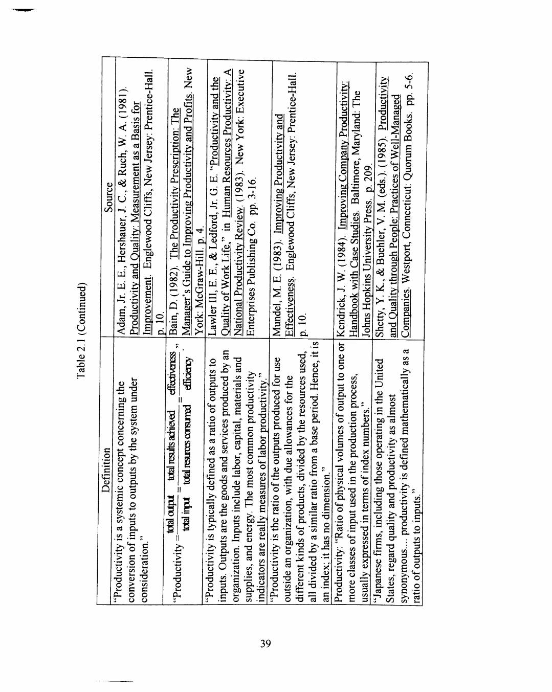
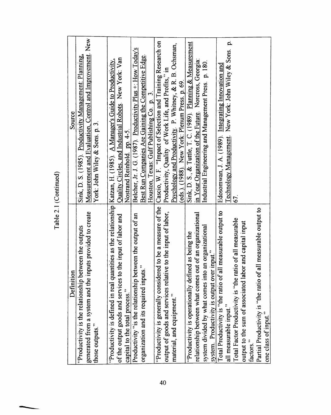
2.1.2.1. Definitions of Productivity
Table 2.1 presents some significant definitions ofproductivity in the open
literature. From these definitions, several points can be concluded:
1. The core definition ofproductivity is the ratio of output to input.
2. Productivity ratios vary in measurement units. They can be measured in
%, dollars per hour, pieces per day, etc. If productivity ratio is measured
in revenue per cost, then it directly relates to profitability.
3. Productivity can only be measured for tangible inputs and outputs.
4. For different purposes of measuring productivity, there are a number of
different measurement approaches.
5. Productivity is closely related to effectiveness and efficiency.
6. The output ofproductivity assumes valuable product or services. That is,
the output does not include the valueless. Based on this assumption, it is
possible to relate productivity with quality.
37

<D •*->
* i » ^
C <u a-o
H—»
5 o 3 o
CO C o
c
38
(U
•4—» c o U
39
3
n o
U
o
3 o
00
t>4 c 'c c c3
c
c
3
o
oo ON
00
(L)
C (U
E > o l - l
D
B -o c
o U
o
>
C aj
• * - •
C U
s l - l
3 (/3
^ S CT)
( ^
en C o
I .§ o
o
u 3 o
0) T3
'3 O
a a >
o
o
X5 o
Vi 3
T3
N 3
Ol
<n
D.
c • 4 - j
O
C/3
CO -o o H
o
+ CO
•4-> o 3
TD O
0 0 ON
o
W
>
s o
U (U
c
O
o U c
3
(U
C/3
'S O Vi
&I
d U
C
3
(4-1 3 O X
H c o +-» 3 o
c
e V-i
3
c 'S c cd
.2 o bO 00 * - < 1 — 1
o ^ cL O
P 2e
^1 ON 0 0 ON
U H
3 H
l - l
3 • < - >
3 PH (D x :
••-» Ct-i
O c o
N ' c
U 3 ^ O
.S
(L>
cd C
c
"C u 0) C
'5Jb c
W
3
C3
c _o -4—>
> O
&4
'•4-»
•4-»
c
Vi c o
0 0
(L>
c x : o
o
O N G 00 u ON g
"-^ 04
< c
I s ^ o S -o o c 55 -G
t ^ vo
c '•4->
'5
Q
-4-» Cd
o -o > o
c a,
(U on
O d
l - l
x : •4-> cn
'•4->
o 3
ID •4-> cn > . cn
e . O ^
ci: 3
0) 3
CL» on O
x : 00
Vi TS
O cd •S »-' ed o
" -s
cn -S
«.s •S -G
2 o CT cn
- ^ 0) cd u
• — cn
S " ^ «« 'O o
cn O
S § o x : l-l > -
^ o
cd
3 •4->
3 O
x : •4->
c
cn cd
X i
cn cn (D
O
Cd •4->
o -4-J
cd
o
cn
-=5 in
cn x )
cd o *
^ • -
s Cd
. ^ § N
x : . *-• u-
® -s <L> i S
• 4 - *
3
o o * ^ •4->
c '- o < x^ ^ ^ 2 <^ <i>
fe ^ £ O C . & 00 cd 3 c« cn 53*
•— "O w >- O TS
•ti o c > 00 ed
x : -•-<
00 c
cd C
'•4-> Cd N
'S cd 00
i= o x> tn cd
(D
IC <D
>^
C _o •4-< Cd l - l <u a. o Vi -^
cd
o
N "S cd 00
>
c ed
c ed O
•4->
cn <L)
E o o
•4-» Cd
-a
3 O cn
s o
X) r- C i i
3
_c l - l
> o
•4->
3 •4-» 3 O cn
i . > -4->
o 3
-o O
3 >
O 3
O c cd 00
DH O
3
O V H
o I d 3 ' C
-S Cd 8 e
3
O
x : cn C o
:C OH
B •4-*
cn
cn
3
a-o
l - l
3 cn Cd
6 cd
O O
'•J3 cd
x :
cn
•4-J
o 3
-O O l - l
— < •4-»
^ 3 ed Q , 3 .B Vi ^ _
?? eS U -4->
6 '5, —, cd
.2 ^ -5 o ed X ) »- ed <u -^
x : -o . ^ (U ^ •4-»
cn . 2 T ^ ^ 9
^ Q_i cn
cd o X
•4->
cn
cn
3 O cn ed cd Lu
O r cn
cd £ ed
o cd H
3 *-'
o ^
3
o
ed l - l 3 cn ed
cd C4-1
O _o • 4 ^
Cd l - l
cn
> 3 • - P O .
O C
o o P i cn — J H . 2 O
cd c D H O
40

3 C
• * - »
C o
U
1 i-
' 4 - '
a (U
B o o w >
Q Of C V i 3
•4->
o
ufa
Man
<N ON
T3 C cd
ity
* « 3 o 01
c *s iJ ed ti <
for
ines
w^^
<1> ^T3
3
c O cn cn (U
_C 'cn 3
CQ
O
c
T3 O O
B ON
'--,_ -
<
(1> C/J
O ffi o s
O • •
ions
rd O
Q
vity
•4-»
CJ 3
-P < OH
E 2 «•> " — g w o O 5= X f i
SH-H cn
3 C M TT; •4->
3 O ^ ed^
O <u /> " ». . ^ cn Wi
td § -o ed »- D H cn ^ - '
y cn (L>
c 3 a> vi I ^ ^ 3 te tn S ^ ed
I i2 -O cd C cn ^ 3 cn
. ^ O ^ 2i
•g -aa ^ S no O- <U - ^ O cd te > ,
cn r r Cd
X C ed o
<C (L) E
41

<L) 3 C
•4—>
c o
Cd
U l - l 3 O
o C
CQ
cn O O
.1 < bilO c l - l cd
c o cn
T3
> • • • I •4->
o 3
B — ^ 3 :2 O
^ . - I
O -S ^ 8
cn C O
00
<^
>J
c X ! o
o
2
cn C cd l- l
H
-4-»
3 O
(L> X H ••-»
c e 01)
c cd
cd 3
cd •4-J
o H
ON ON
( / )
ed
#N
CJ
cn C
2 QQ •4-> cn ed
w m 00
^ ^ c
CM a
U C cd
a l - l
<u P H
01
c " > o
3 S
O 5
00
c X cn
3 3
OH cn
X o
9 >. cn
<D X H
S O H -<
m ON ON
w J
cn r! 0) N Cd
^
c/i P
o cn M O
cn C O O C/5
^
cd ^
S cn cn cn U
o 1 ^
P H
^ '-^ rd 3
o o cn c>
C cd
:s
" ON
. iX
vi Vi 4> l - l
- ^ cd 3
a o <
T3 '3
o (U cn
• 1 - 1
O c o U
cn •4-»
Q 0) u C o
U cn cn (U
_C ' c75 3 m >i
m
00
•4-»
3 O
pi:
o
2
cn C ed
ON g
' — ' l - l
^-^ (U
i2 -l - l
T3 C cd 04
(D C
'53} c
W
o 3
-o o
a.
cd
o
Vi
^< o
ON ^
"5 c
c s oo
cd cd
B ^ 3
00 cd
o
c
T 3
O cn
cn O CJ
•T3 C ed
B
o >
c -4-> o 3
T3 O Vi O.
C4-( O
• 4 — • •"
.2a ^ o > 3 '.S
cr o
cn
urc(
o cn 0)
CQ
3 U Cd cn (U o
Pij
3 O ,
^-> 3 O
T3 .4->
o r Cit s X ^ W p Cl. •
O 3 11 - g
o o
^ ^
P H W X
3
o cn (U
P^ 3
t O
3 • 4 - *
o 3 O ^ .
" 6 3 3
< o
.I.S Cd O
<L> ^ Q l l - l
c ^ ed TS
C i - . t i
- X <u -»-; >-' Xi
3 «4-i T -
C tM 3
s Id I 3 X >
: > > - | ^ - > •4-> " ^
o o +_ 3 3 3
- 0 * 0 0 O C X V - l - l . * - >
PU P H • >
00-]
o
3 cn (L>
X
x:
X 3
3 D , +-• 3 O
•4-< ^ ^
B- 3 3 O-O . C
•4-» '
o '^^
( 4 - 1
o cn cn
,2 I j (U c o
C4-I
o
ed 3
I
.4—• ^
ed l-l
a> X ^-> cn
: > ' c n .*-' Ui
o c2
Id g" o •'-H z= i ed
V H . ,_,
•s§-^ - r i
•% o
p ed
C ^
c^ld ^ • § +-» o O V, ed cn
Pu ed -1, ^ cd O
S cn
3 •4->
3 O
o o
• 1—1 ^-> cd
X
cn
•4->
3 -o O
Cd ?
'i *=
42

2.1.2.2. Definitions of Quality
Table 2.2 provides the important definitions of quality in the open literature.
From these definitions, five points are worth noting:
1. All the definitions in this table show that quality is an abstract term, and
is not measurable.
2. Some (e.g., Pirsig, 1974) believe quality cannot be defined, while
others believe that it should be defined by situation (e.g., Deming,
1986).
3. Most definitions demonstrate that quality is customer-oriented.
4. Quality can be defined from two aspects; external and internal
environment. Definitions related to the customer are defined from the
external aspect (e.g., Juran's "customer satisfaction"). Definitions
not related to the customer are defined from the internal aspect (e.g.,
Gilmore's "conforms to a design or specification").
5. No definition of quality in the open literature was found to relate directly
to profit.
43

l - l 3 cd l - l
c
O
x ;
cd 3
cn
o
c u Q
cd H
O Vi 3 O
00
o
c o
C4 e o
U c cd
cd 3 Ol.^
ON
I
NO
a a cn cn <U l-l
cn Vi
>
HJ .2
o X) X5 <
a
ed X )
B o
U
o Vi
•4 - J
c o
U
cd 3
o •4-»
o H
ON O H
> X
cd
o B 3
^ ^
00 i :
O 3 '—
'O O O '— Vi
P H Q . <*H
o 6 Q
J? >
so > ON <U
cn •—t a>
'^ Vi
Mi (L> ed 3 3
c o
U
cd 3 o
<N
a, a.
.§ s cd l - l o
"^ v« ' ^ O
X <u
I
Vi O
C
•-» o
2 C b ed
cd 3
Ol
cd 3 a
( 4 - 1
o 00 c
"H cd
a> x : H
V , •4->
Q9 u
r Vi Vi T3
Vi cd
W pu o
IS >\ o Vi
o •4->
o
o
00
PU P H
cn J^ o o
6 ed
•4-»
c cd
CQ
X
C cd
c N o
. > ^
r^ (L>
.-^ ^
Pd g
V - ^
PU 2
o O ci o
T3 C o
ed 3
01) 3 O
o Vi
PH
ON NO ON
C/3
00 V i
a> X ) c (U
^
<N
, CU
cn cn <U V i
P H
cn O
U O c ed
C o
U ^ - : 3 ^
- a ^ 2 OJ
PU ^ 3 (u
. c / ^ 3
^
J
ffi r»
(1> V i
O B
773
cn cn W & O V i
P H
,> -4->
'CS zi
O Oi
c o
c
c cd 3
cr X
cn O c Vi »-
O ' C
3 fe
cd a>
•ti <u
.s-S OJ cn
C ^
(H £ «t2 o • - 1 t/5
cn
x ; H cn C o
c o o Vi
B
(4-1
o
o
o-00 c cn
x :
cn 3 O
Cd
t : o
cn (U
X cn C cd
cd 3
73 C ed (U cn 3
3 •4-J o cd <u
x :
cd
>-> P C d ^ •
cn O C= ^ O t 3 :5 2 TJ O.
CJ •4-»
ed D
2 ^ 3 f ^
W cn
^ B
^ O -£- cn
V - ^ - .
ed •'-
Vi
D
cn •4-» ed cn
- 4 - "
o 3
T D O
rti cn
0 ) < i
a, cn r ed
CD
(D U
® X Vi ' * - '
"cn 5 >-» O
"cd 42
^^ +->
c P
o o
0 ) VM
cn
C O u •*-' o 3 o Vi D .
"5 C l , cn ed
X o
X )
^ 1 = ;
&) o
X cd
Cl. a
cn
cd 3
cn •4—>
c cd
x :
X " •
^ o o -.p -^ cd
febo <U 0)
73 CM <^ ^
" gj ;_-- (U cd t S 3 cd
cn •4-»
c cd
(^:^ cn
•4-» ed cn
U cd CX ed o 4)
X
o cn
•4-» cn
• n cn C o
ed 3 a
o c c cd O
S ^ X •4->
ed • * - '
3 X Vi U
-4-> •4-> Cd
B Vi o c
Ti
c
Vi
o
3
a. cd
' t l p
cd 3 cr
X 00 3 o
X c >
3 cn o -•
B O c o u
cn
O cd X e ^ ^
cn •4->
3
'C ed
o
cn O
X •4->
c cn
cd 3
X
C
C
cx 73 C
o c 3 o
r
c
-73
•*-• cd
C L
s 3
s X cd £
X
•4-> D
cn > <D (L) > X
• Si O X ed ^ X
o o ed
cn
Cd 3 a
^1 ed 3
B 3 s
cn O B-
_ 3
o ^
X c cd CJ
•o c cd
(U Vi 3
T3 C <U
X - ^
Vi C ed O
^ B (U Vi
-^ c2 • 4 ^ M—I
V- (D fO 3 T3 2 OJ -^ Vi <!->
^ X ) .. ^ ^ «* O TJ
Cl, t3
•5 T3
cn
C o o
-4->
o 3
T3 O Vi
O , O o
cn ed
X CJ
> C ^ O O -42 * - cd (U o
*T3 O j
«> !^ •4-> O
^ V, •^ (U cd " H 3 Cd a
44
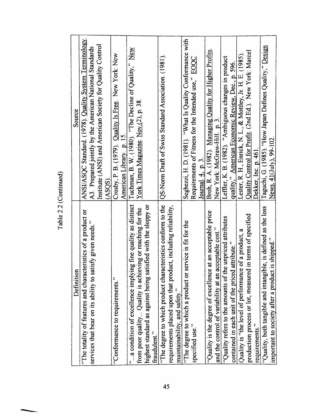
OJ 3 C
a o U
<N JJ 15
cd
H
CJ V i 3 O
0 0
P H =5
o
<u V i
tlH cn
ed 3 a
ON
ON
m
X5 cn O Vi
u
«o
cd
c cd o V i
B <
2
ed 3 a o w C 0 0
<U r v Q ^ X 3 ^^^ ^ > • i O
ON -ia
. 00
CQ cn
C B ed • -
S ^ X ^ =* P
00 ON
c ,o •4->
.2 o o cn cn
<
ed - O C ed
• * - >
(/5 cn cn
cn < 4 - l
o
cd
o I
CT)
O
0) CJ C! cd
a c o U
cd 3 a cn
u o o PU
OJ cn 3
T 3 OJ
T 3 C
ed
oo ON
Q
0) X
cn cn (L> C
•4->
o cn
•4-»
cn
CM
rf S N N <U
X 0 0 <D
C/3
(U - U ed
e 3 O
3
D
cn •4—>
o
OO
^
ed 3 o 01
c 3) cd c cd
0 0 ON
X
o V i
03
cd V i o CJ
V i
o
CJ 3
o
cn
0 0
ed X o cn 3 O 3 Op
6 <
NO O N
cij r
Q r
• >
OJ
CM OO ON
V i
H-I
B o c o CJ
w c cd o
cd 3
al
oo cd
o
<i^
V i O
T 3
w t 3 C
CM
^ 2
"C fP
K g
(u ;:= tn § J Ol
01 cn
Q
cd 3 a cn (l> C
ic OJ
Q c cd O l ed
•—> ^ O
NO
CJ
Q
oo ON ON
O N
O
3 ^ 0 0 ^ Jd «
H :z;
c o
c
Q
TS Vi 0 ' O Vi <L) 0 1 a> ed C
>
y 0 0
Vi cn
cn CJ
o ed V i ed
X CJ
^ 3 C ed cn
Cd
cd cn
O •4->
cn
o Vi
cd
X > O
^ ^
^ ^ •4->
o -4->
x: H
cn
CJ
cn
cn
£ V H
"3 cr OJ
OJ CJ
c Cd
C o U
•S X -t-> •*-'
. 2 2 « --o a
;^ o Cd Cd 3 JJ a- ^ c o
- 3 D
^ X O . O
J »
c is
X
c "2 ® S-
o Cu
o, "cn
X
T 3 QJ
Vi
ed cn 0 0
' S x> cn C
• »H ed 0 0 ed cn ed
(L) ^
5 S c .2 a •-c op o c cn 3 O — cn C
•4-> O
5 -o ed p
o. X O
ix Vi O
o, o, X =5 CJ 7 3
- 5 t j ^ ed
a cd cn
•T3 C cd
c o O cd
cd • ^ . C - . cd -4-;
cn 3 JJ ^3
X3 3 Op 5
i : X ^
o o- ^
o o o, £ o
o cn
T3 2e
^ '5 n cr r^ OJ
X ed C
"S •4->
c
£
X
c2 •4-»
cn
CJ
cn
CJ 3
T 3 O V i
O , cd
X o
X
o ?
00 "O -O I -^ 'o r-' u H o, :{ cn
OJ CJ
^ cn
CJ (U
^ 8 OJ ed
§ § ed
X i
.2 cd >
CJ X OJ
o •u
-I .22 o
-73 -C ^ T 3 a c
:J cd
cn OJ
•4-> 3
JO V i ti ed
CJ •4->
^ ^ C Vi 3 ti D ed
X T 3 < -i CJ
«5 a
3 X
cd ^
X '5 O X
^-> CJ
22 S
(U • — V i ^
1 " a o
7 3
ed a>
. O H
-4-> cn
3 ^ ^ s o « Vi C a w o .£
c2
V i 3 cn cd
„ £ O- o
gj cn > cn (U OJ
—' o a> O
- C Q .
.22 o
^ 2 a O H
cn cn
X •4-> cn cd
T 3 <L) ?
-o cn
. 1 - 1
OJ
^ - ^
00 g § - c 2
TS cd C „
0 0 ^
OJ CL
o. X
cn cn
cd
cn •4-> c OJ
£ V i
'5 al
CJ
o cn O (
X5 -*
> S
i a Cy B
45

(U
3 C . ^ 1 •4-» c o
U Csl
CNJ
a cd
H
CJ V i 3 O
C/5
o 3
T3 O V i
P H
3
o cn
' V i
OO Cd c ed
0 0 ON
ed >
O
2; cn
• • - •
O X) o
p^ I d
cn 3
-o c
T3 C cd
r
cn
Cd 1 ^ N - ^ ed 3
^ Ol
O x : c
"S Pd 73 C cd V i
•4-J
cn O
2
NO"
a -§
w (JO t—I . 3
Vi Vi
' »-i V i
u X
3
o cn . 3 3 00
X c
ON 5 O
>• i < > ^ V i
00*5 ^
l i f e OJ ed (L> Q S U
o
cn cn (U CJ O
a OJ £ OJ > o Vi
O
£ I—I
<u X H
o
2
cd 3
> o V i
O
£ l - H
cn OJ
'£ . cd
'TT Cl ! I OO O ON U i;2- 01 t-yH Cd H U 0)
to n .£ 'C t c cd q
ON
I
ed V i
o CJ
cd 3
o a cd
CJ 3
73 O
ON
00 Pu
00 t oo p ON > - l
< z.
> o
£ o cn O o
CJ 3
o
c _o •4-»
'S 0)
Q
cd t ( - i O cn <U
•4-> 3
j O V i
ed C 4 - 1 O
,^
I d •4-»
o •4—>
0) X • • - •
cn Cd
73 d) C
OJ 73 cn
cn C OJ
. ^ 00 0 0 . C cd 'Sd
cn • . p OJ ed X )
O cd
^ cn
O H . Cd C O O
"S 'c C OJ
•-- T3 H-> QJ •-* >-»
c ii O OH
d> ed
O H ^
o "ts OH O
ed 3
o c/)
r . ^ ^ V i
-3 o
cn »-•4-> CJ 0) OH cn ed cn 3 O
QJ 2
3 O
cd 3
o ^ ^
cn QJ cn cn Q> V i O H
X QJ
5 ro . 15 3
o c' v i o p cd
£ ^
2 &
§ . 2
cn c
'C B <D 5^ -ti T ^ V i
cn " S CJ QJ 3 £ B
O H ^ QJ
Q^ CJ
QJ c/) «n
ed cd 3 O cn
Ci U H « cd r^ ^
cn
> +-» CJ
x* o
73
cn QJ
.'I cn
. ^ 3
o NO"
x> 73 QJ X
cn
73 C ed cn Vi QJ <D C
'53) c u
X 73 QJ
0)
22 ed
x: CJ
cn C cd
C 3 O QJ
••^ 2 P CJ w
O * -
0 . o
cn" 5G " 5
QJ
X o
X 73 C ed
C QJ QJ
^ ••-» Q>
X> ^ • H
3 QJ
U QJ
ea X
O ^•^ 00
O . 3 QJ ' 3 ed u
QJ cn 3
X ^ cn QJ
QJ
o 3
73 O Vi O H
ed
QJ cn O
e-.
^r td <C =» c
• o" o CJ cn « - i QJ
<U ! < 00 QJ
cd 3
o
CJ QJ - X QJ £
o _ tM QJ ( /3 0^ O X> :J
3 cd o
QJ
QJ B is on ro 3 cn U g Cd
• - 1 cn •4-» -4->
• 5 ^
?> ^ 7 3 Vi
QJ 73 ed
3 O H
73 QJ
73 C QJ
e &2-S QJ
X
QJ U 3 cd
V i
. 0
3
•4-»
c ed £
73 C cd
3 QJ
QJ X
QJ X -4-»
cn 3
£ •4-> 3 QJ
iJ
3 •£ O
QJ c^_r •4- QJ
cn QJ
*" a ^ ^ •^ 3
4i •ti -t^ "* cn
i « 3
73 QJ
" > O
QJ O
2 X > o ^
cd
.2 >. •:: ts Cl -4-f - r : »T-« T \ «-! —
X 3 .4-> . 3
* - rt ^ ^ cn <i>
• * - >
cd O
73 3
a 3 o ' 3
cn
X > cd
' ^ I j
cn 3 00 QJ
X>
. ^
3
o
QJ X H
QJ £ QJ 00 ed 3 cd
£
cd 3 O O
5 QJ 0) 3 O H I C cn QJ
- 73 cn 3 « cd X> 0 . C O CJ
.£ ^ ^ _. v i Cd QJ 3
"£ o O :J
73 CJ QJ 3 fa -n
I 2 QJ * "
X I ;2r cn ^ ^
QJ X
o X
CJ QJ O H X
•t: . t : . t t x X £ - 3 "3 o ^ 5 'cd .^
O ^ i O H
3 ii
QJ QJ -fS X
QJ cn
3 cd
5 -O H
QJ ^ CM S
o o.
• £ - ^
i3 X) 73 i S 3 cd V i
QJ
QJ f -cn -r; 3 >
ed > ed cn
-t-; O • - -
52 oJ 3 CJ QJ
ed X
cn O CJ cd
• • -» cd cn 3 O
•4-» Cd
•4-> CJ QJ O H X QJ V i
QJ £ o
•4->
"^ B .£ J5 •S "X QJ O QJ -^ CJ QJ X 3
o > 0 0 ^ 3 c
^ 2 S CIH !f=H (U
^ • £ «4H O , O cd
_ V i cn (J
B ^ t cn QJ cn - ^ QJ 3
QJ cn 3 Vi
cP M—1
cn (/J QJ S - 1
•4-H
V i
n
rew
cn cn QJ
X
•4->
0 -J
73 - 1 -•-» o
UH - ^ vi 2 > OJ
46
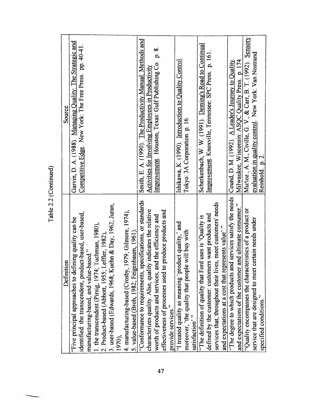
7 3 QJ 3 3
•4-» 3 O U CM
CM
a X ) cd
H
QJ CJ Vi 3 O
3 cd
01 QJ
•4-> Cd V i
-4-»
OJ x: H
ed 3
o
cd 3 cd
I o ' ^
o-o. cn cn QJ
QJ QJ
QJ
x: 01 H
•3 T^ o
QJ
0 0
ON {jij
w < QJ
• o t B ed O
o u
73 3 cd cn
T> 0
X ••-> QJ
* « 3 § S ^ : >
•4-> 0 3
73 0 WH PU QJ
X H 0 ON C3N ^^
<
W X
£
^ >
•4-< CJ 3 0 V i
PU 3
cn QJ QJ > 0 0 £ 01 ri > 0 > 3 t—(
V i
c2 cn QJ
•*-'
> -t-i CJ
00
0 ,
0 U 00 3
X cn
Xi 3 PU
tVH
3 0 cn ed X QJ
H §
•4-> cn 3 0 3C •4-» 3 QJ
£ QJ ^ 0 Vi 0 £
3 o U >\
•4-> . —
3
3 O
" • * - •
O 3
7 3 O
NO
3 O
o ^ ON o
^ & ^^ o
ed O ^ >-% • 3 - ^
X o ^ H
ed 3
•4->
3 O
U
7 3 ed O
pci cn
QJ
Q
NO
cn cn QJ
U P H
£ <u cn cn QJ 3
. , 3 ^ H QJ ON H O N «V 1—I QJ
. o
^ X * J 0 3 Cd QJ
« i vi O Q> Vi
X gi c-> S
o cn 3 QJ
C/5
ed 3
QJ
B 3 o cn
* V i
7 3 ed QJ
CM
cn cn QJ Vi
PU
.§i Id 3
o u o 0 0 <
/ ' ^ cn oa 3 ON O ON CJ 1—1 cn
QJ QJ
3 cd 7 3
3 3 O U
CM ON ON
H
fc: ed U
T 3 3 cd V i
• • -» cn O
3 cd
>
O
QJ
z > -d
o #N
QJ 3 O o
> ^ > ed 3 a CM
N O
3
3 O
> QJ
O X .3 "S P
7 3 3 cd
cn ^ • ? cd 3 =3
cn
O r-
7 3
O i i O H ^ ^
00 g , .£ ^ c 2
ed 2 ^ 3 ^ a -
s "I ed O t ^ QJ QJ ^ Vi VH . ^ - o -5
f 3 ed :: 3 cn
cn T 3
QJ QJ
cn -g C
>. «« 12 t i cn QJ
3 ^ 0
O ^ V i - ^
cn O , CJ • - * -4-J •<-•
« 3 3 « Cd H 3
-o V i O
O
g £ cn QJ
cn QJ
P C > (JH 3 X
2 u. cd
x: cn QJ
•4—> - ^ _ C -4—>
QJ
> cn
•4-' 3 QJ cn <i> V i
CM QJ
ed X!
cn 7 3 QJ QJ 3 QJ
X •4-»
cn •4-» Cd cn cn QJ CJ
't QJ cn
-o 3 ed
QJ
£ 3 cn 3 O CJ QJ
•4-> Cd
7 3 3 ed Vi QJ
42 £
3
3 O
Id " 3 ^ — or o 00
C4-1 c n O =3 „ 3 ^ X O <U * ^
•»H J ^ " • C » • = t s •-3 ^^ ro C > > X
IG X *" QJ n - l C/3 '-' QJ CJ QJ 3 - ^
H JJ 5 i 7 3 cn
cn O CJ cd
cn 3 _o
S t j QJ CM X QJ
7 3 3 cd
o 3
7 3 O Vi
O, X
CJ
x:
QJ QJ feb QJ
7 3 QJ
X
H
cn 3 CJ QJ
x:
cn 3 _o •4->
ed -4-> o QJ CM X QJ
7 3 3 cd
o 3
7 3 O V i
O -ed
cn O
' • • -» cn
'C a t j cd Vi cd
X o QJ
X -4-> cn QJ cn cn ed O H £ o CJ 3 QJ
ed 3
o
QJ 7 3 3 3 cn
7 3 QJ QJ 3
cd
t : QJ CJ
• 4 ^
QJ QJ £ o
-4-> 7 3 QJ
• —I cn cn c
-o •-V- T 3 cd 3 ^ O cd o
• £ T 3 <1 £ CJ y ^
C QJ QJ O H cn cn
47
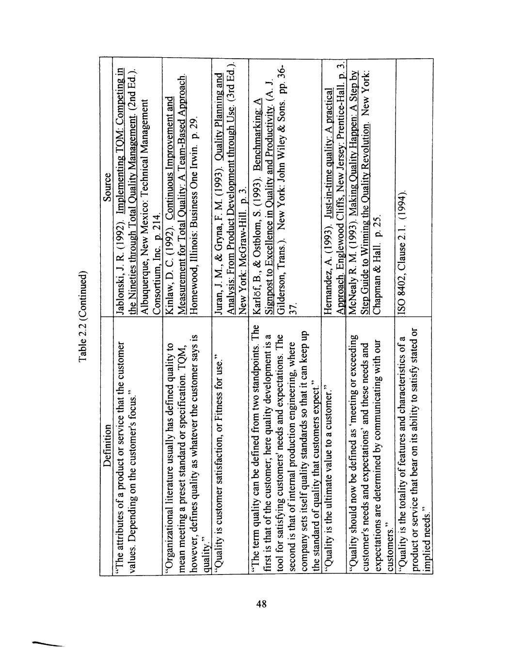
T3 QJ 3 C
' •4->
3 O
U CM CM
a JO cd H
QJ CJ V i 3 O
01 _3 •4->
QJ Oi £ o U
: ^ ,
H ox 3
•4->
3 QJ
£ a "ol
t 3
w 3
CM
3 QJ
£ QJ
ed 3
CM
ON
pci -£
^ QJ 3 •-H
JO QJ
^ x:
3 QJ
£ QJ 00 ed
^ C 01 i 2 3 ^ Cd
o "£ x: o OJ
H d CJ
'x QJ
QJ
z QJ 3 a* V i QJ 3 a* 3
X5
ed • • -»
O
H
oo 3 O cn QJ
CM
O 3
£ 3
o cn 3 O
U
73 3 . cd
8 QJ
£ QJ > O
cn 3 O 3
. 3 •4-J
3 O
U
CJ cd O V i O O
T3 QJ cn ed
CQ
£ cd QJ
H
cd 3
O
H C J ON ON
^a u ^ Q £
cd cn - 3 cd 3 <D
3 ^
ON CM
QJ 3
o cn cn QJ 3 cn 3
CQ
• wm O 3
O O
QJ £ o X
3 cd 01 3
'£ 3 ed
cd 3
w T3
V i
QJ cn
00 3 O
m 3 QJ
g:: ii ^-" I J ^ >
Q Pu ^
^ CJ
2 =3 3 T3
^ 2 O Pu
£ .• 2
cn ^ - ^ 3 * ^ ^
<i^
cd V i
3
cd 3
<
O l
cd Vi o CJ
o
QJ z
3
V i
Cd
CJ 3 QJ
OQ
CJ 3
73 O V i
PH
73 3 ed
ON §
Coi C/3 . C
3* <1> 3 O O 3
:Ba -4-> ^—»
cn QJ O CJ ^ X
- o c4-r o : 0 O
NO
OH O.
cn 3 O
00
<^
QJ
3 X O
o
QJ
:2;
cn 3 ed
3 O cn V i
QJ
5
<^
O H
^ J
ed CJ
• • -> o ed Vi O
^
cd 3 a QJ
£ •4-»
1
3
Just
-1
ed
X QJ CJ
3 QJ 1—
PH
rse
QJ
QJ
:z;
Clif
fs
X)
o QJ • 4 - I 00 <
en:
o
Hap
cd 3 o 01 3
.Mak
ON o ON ^
"^ "ob < c QJ X
73 CJ 3 2 ed p
QJ O^
ON ON
O
QJ
:z; 3 O
O > QJ
0^
Cd 3 Oi QJ
3 3
'ed
>^
QJ
CJ
QJ 73 3 o
•4->
C/3
c^
3 cd
£ 9 t ed
X CJ
ON ON
CM QJ cn 3 ed
u CN o "^ 00
O C/3
3 O
3 it: QJ
Q
QJ £ o
-4—>
cn 3 CJ QJ
X . -4-> i-
"3 ^ ed 3 -a ^ o QJ fti . y cn
^ QJ
O cn
O cn * - 3 o o
O . ed
3 O 00
o .£ cn "O QJ 3
re ^ ed cn
x: a H ed
o .^O I d H
Ii 3 CJ
QJ ^ t : 7 3 CJ
QJ J8 O H 2 cn
- ^ I ->-, O
l - H 3 ed cn T 3 =5 3
2 -2 3 ^ -*ri -•-* Cd QJ Vi cn QJ QJ
X : OH I d «* 3 00 .2 .£ ed QJ N QJ
•£ £ V i ^ ?i
Vi
Vi
cn V i
QJ
cn 3 CJ QJ
X
QJ > QJ td
I cn ed
ed 3 a-cn QJ 3
IC QJ
73
QJ . t : ^ I d o E. X a"
x; ed QJ cn - ^
O H 3
cn •— ^ QJ
QJ cn 3
cn cn QJ 3
• » - i
V I
o 3 O
V * CJ
<iH cn
. ^ 1 •4-» ed cn Vx QJ
cn 3 o cn
cd 3 o
o O H
73 3 cd
•4-»
cn
3 cn « 3
£ .2 o .2
I J CJ > QJ
73
o tVH
73 QJ 3 QJ
73 QJ
X 3 cd CJ
QJ O H X QJ
73 : 3 3 cd cd
a" 73 Q> QJ v: QJ QJ 3
- ^ -cn
cd 3
QJ
£ o —> cn 3 CJ QJ
x:
QJ £ o
-4-> cn 3 O 00 3
„ OH
X <i
tc 00 ed 3 « •c .ti QJ ^ gj ed 3 X sbr: 3 ® Q3 '^
O vi
CJ ~ ^ S - ^ « O Vi Vi . O H ^
00 . £ 73 73 3 QJ Cd
X QJ
CJ QJ O^ X QJ cn V H
QJ
cn 3 CJ
•4->
Cd X 2 Id *-
QJ c r
c ^ ^
t = «+H 3 ff:
• ' - Q J C4-1 c n
O . t i ed
QJ ^-> QJ
X
H
C> .22 r -• 3 "S " ^ ed ro
X ! ^ - ^ V i
cn , 0 •—H (4—I cn o
U-* •4->
ed 3 al
14-1 o 73
Vi cd
73 3 cd Vi QJ
cn CJ " f f
cn . n 73 3 O u
Vi • * - »
QJ cn
3 cd O ,
£ o
QJ
£ o
••-> cn 3 CJ ed O
•4-»
QJ > QJ
£
QJ X •4->
cn
cd 3 o
»- 3 O
QJ 00 cn 3 <L>
•ff - ^ QJ 73
Eg ' cn 3 O
•4-»
Cd
3 O
X
00 _3
ed CJ
' 3 3
£ £ o o x>
cn cd
73 QJ 3
i ff t> " ^
^ OH 3 QJ X C
x> <i E
2 «J C cn
73 T3
QJ •4->
QJ
-a QJ
3 SJ «*
cn .2 CJ cn
QJ 'ff
o X cn J cn
cn 3 O
- ^ 3 « X 3 •*-'
o a ^ o s & ^ CJ QJ
cn V i
QJ £ o cn 3 O
CJ ed V i ed
X o
73 3 cd cn QJ
cd
a O
_^
•4->
o • * - '
QJ X
cn
ed cn O
•4->
X ) cd cn
3 O V i ed QJ
X i •4->
ed X QJ CJ
QJ cn
3^t^ cd 3 o
cn 73 QJ QJ 3
73 QJ CJ
3
-o ^ c O - . 3
48
2.1.2.3. Definitions of Profitability and Profit
Table 2.3 presents the definitions of profitability and profit. From this table,
five points can be summarized;
1. Profitability is directly related with productivity.
2. Quality is not directly related with a measurable profitability.
3. Profitability can be measured in terms of various units.
4. Profit and profitability are similar terms. Therefore, unless specified in
models, profitability and profit cab be viewed as interchangeable terms,
especially when comparing the relationships with quality or productivity.
5. At firm's level, profit is the result of all combined efforts in a company.
Therefore, unlike productivity, no 'Total-Factor Profitability' or 'Partial
Profitability' is found in the open literature.
49
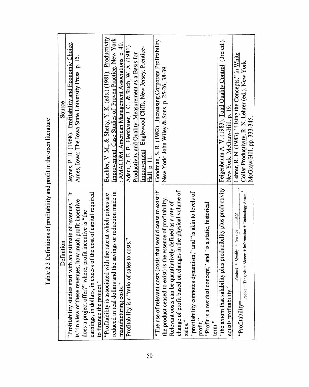
QJ Vu 3
• • ^
ed V i
QJ
3 QJ O , O QJ
x :
Iff o
73 3 ed
X ) ed
•4->
Iff o
cn 3 O
3 Iff
QJ
Q
CM
i i X5 ed
H
<u CJ l - l
3 O
QJ CJ
' o x : U CJ
'£ o 3 O CJ W -o 3 ed
X > ed
• 4 ^
Iff o
»ri
cn cn QJ V H
C U
.§ cn V i
'£ O QJ
• 4 - >
Cd • * - >
00
rd ed
^ . ^ P H O
^ •—' cn « Q> cn
>> £
CJ 3
o
o
QJ
QJ U
ON 2 OPu . - V 3
p^ t ^ C4
> ^ cn - 2
QJ ff X 00 ^ QJ
<^ ^
QJ
£ QJ > O V i
X „ OJ O
03 £
o
cn 8
_o • 4 - »
ed CJ O cn cn
< ^-» 3 QJ
£ QJ 00^ 3 ed
3 cd CJ
. 1 1
V i
QJ
00 ON
<
X CJ 3
«N
u
QJ 3 cd
X cn V i
QJ
X w
£ cd
73 <
a Vi
cn ed
OQ cd cn ed
• 4 - >
3 QJ
£ QJ V i 3 cn cd QJ
cd 3
o 73 3 ed
o 3
73 O
I QJ CJ
3 QJ
QJ cn V H
QJ
QJ
z u 73 O O
J[J
"ob 3
W
3 QJ
£ QJ > O V i O
£ cd
X
>i
X i cd
Iff o V H
PU QJ Cd
O U OO 3 cn ed QJ V i CJ 3
m oo
* N
NO CM
I
CM
cn 3 O
00
^a
3 X O
pci
c/i *">
cd o £ >^ o ^ O QJ
O Z
•T3 QJ
73 V i
3 O
U
ed 3
Ol "ed •4-rf
o H
ON
oo X ON i-C ^-^ ^
. ed
> o B ^. cd *s
-^ P 3 >^ 00 ^
QJ • 4 - >
X
^ o .£ > ^ . ^ cn QJ -^z QJ CJ .^-v O Q>
u ^ QJ a> •^ is -^ X 00 <i>
.£ ^ I
).'
(Ti 00 ON ^^ N , ^ ^ ^
:z; tti
rer,
X QJ
Pd >H
• 4 - J
> • 4 - »
CJ 3
73 O V i
O H
lar
Col
m
o M i
^^
Hil
^ ed V i
o
3 O
3 Iff QJ
Q
cn QJ 3 3 QJ > QJ
O QJ
• 4 - »
ed £
• — H +-» cn QJ 3 ed
cd
QJ _ > •¥->
3 QJ O 3
QJ U H
'5 a* QJ
0 ) Vi
^_, cn Iff " "
o,"ff
£ •-
. § 1 S 2 OJ ^
o. cd o
-^ > ^ QJ cn QJ
3
cn
C/5 f W
X5 C d
^ - > Iff O
t ( - i
o
QJ ' > 3
CJ QJ
"o* V i O H Cd cn QJ
-22 •§
cn O CJ QJ
X -4->
C4- I
o cn cn QJ CJ X <l> . 3 " •
. 3 -^-^ Vi <U Cd O
^-— V H
— o. 73 W
^ x ;
""^ 1^ cn O ^ S C Cd 3 ^ E ^ cd o QJ +5
QJ . £ V H
ed <i>
<u 2 a B OH g
.2 ^ > QJ
^ V i
QJ O
2 00 3
QJ -ff - ^ ^ X ^ . t i « ^ ' ^
73 T3 QJ 3
.2 cn , CJ v-O ed cn cn cn Q
t i -<
^ ^
cn •4-J cn O CJ
cn
a cn
C 4 - 1
O
o
ed _
•" ed QJ 3
. »«H
cn -»
cn O CJ cd 00 Vi
.-ff 3 X ) " " ed T3
, t : <u C4-1 C J
o 3 P^ CJ
CJ
3 3 cd
Iff O
QJ cn cd QJ O
3 O
• 4 - »
Cd X • 4 - > cn ^-> cn O CJ
Vi
Vi O O
3 cd >
a I J
V i
O QJ cn 3 QJ
X H
4-> " < ^ O " - *
4 - ( . — H • 4 - ' rr,
X o S QJ B td O ed
"o -« QJ 3 W ?ff S CJ QJ -rt cn ^
S ^ X . ^ • * - » • 4 - >
Cd
t i - i o QJ
£ "o >
C 4 - 1
o cn QJ > QJ
ed CJ
cn
VlT 3 cn ed
"x ^
.4-> J^
73 3 QJ ed cn CJ e« )I QJ ^ CJ cn
.H- O CJ CJ
a •>-' • O 3 O ed V - >
O . QJ Sa "cj
•5 Pd
cd CJ cn >>
X O H
QJ XJ
cn QJ 00 3 ed
X O 3 O
73 QJ cn ed
X i - 4 - "
Iff o
Q J .V
00 ' . C cn
§ a X ed O cn
J4 cd cn
73 3 cd
£ cn
'£ cd 3
73 cn QJ
-4->
o 3 3 O CJ
- ^
o 4-> cn
. —H
X
CJ
Id cn ed cn
73 3 ed
O H QJ CJ 3 O o ed 3
73 . »— cn QJ V H
ed cn
o Iff
:J O H
Iff ^ O £
QJ
>
"o 3
73 O V H O H
cn
" O i
CJ 3
73 O V i O H cn 3
"o.
ed "
"3 ^ •4—> • — H
ed X X Cd ••-• ti 3 ^ £ o .2 fej
QJ 2 •5 o l :j QJ
+
u Vi
<
o H
C o
c o
+
'ci c CO
H + u
o CL,
X ) cd
• 4 - >
tff o
50
7 3 QJ 3 C
^—> 3 O
U
m CM
a X i ed
H
QJ U V i 3 O
OO
> ^ 3 cd O £ o U 01 3
'> O Vi O
£
ON
-^•^ 2 00 o '^
.£ OH
W cn
OQ « cn ^ QJ
-3 3
•4->
QJ cn cd
U
OO <3N
O O
X )
3 cd
X
o
7 3 3 QJ
CJ 3
7 3 O
cn V i QJ >
'£ D cn 3
J^ O H O
X Vi 3
X O
>—> QJ
X ^ H 7 3 3 ed
* & ed
QJ O
P ^ P H » n
+ T
CJ cn 3
7 3 O SI
O H ^^ II .QJ
. ^ ^ a pci - O c/5 ed cn
<H S O " -^
3 CQ
^ - ^ ed
• «N
Q b .. QJ
> O CJ
2^
QJ
01 3 •*-•
3 QJ
£ oO ed 3 ed
o 3
7 3 O
3 QJ
£ OJ > o V i O
£ I—H 7 3 3 ed
3 O U
r 3
_o '•*-' cd
>
0 0 3
QJ
^ B Q S
« cn -ixj cd £ .2 bo S
cn 3 O
0 0
< ^
QJ
3 X
O
o
QJ
Z
o
+ Vi 3
CJ 3
7 3 O
QJ >
QJ O
£ o U QJ
X •4—»
oO 3
'£ o
Vi
QJ
^ - v e d
oo £ ON O
- u
^T 3
cn
V i QJ
^ CQ QJ - v ^ ft QJ O
ON
o U 0 0 3
• »—
x: cn !5 3
P H
c+-
3
o cn ed X QJ
H 3 O cn 3 O
01 7 3
w
3 O
• ^-< • ^ - »
•£ Iff
QJ
Q
cn 0 0 3
ed QJ
£ o 3 O CJ QJ
CO
« 6 D u
3 73 O V H
O H
oT VH ii •a
D
3 O
3
•4->
3 O CJ
o QJ +-» Cd Vi ed
cd ^-> Iff O
• ii - . >
3 -C cd { i , 0 0 X
£ > X) -^
O ^
e« A: Vi O^ QJ II O . ^ Q> : =
x : -2 ^ ^ • H
3 ' ^ 3 O
P H Cff S
<ii > O
o
o
•c P i 73
a> CA
D c ed 3
a 2 o
C/3
C c4 3
a
QJ V i QJ
x :
QJ > O CJ QJ V i
QJ O
Q cn QJ
cn
+
7 3 O
"C QJ O H
7 3
_o QJ O ,
3
*ob V i ed £
^ — > Iff o
V i O H cn cn O
QJ O 3
7 3 QJ
5ff O
QJ ^
QJ
a &) QJ
X
^ • =
o 3
T 3 O
3 O
. 1 1 .4-»
3
o o
ed cn
•4->
QJ 3
7 3 QJ
7 3 QJ
•4->
Cd ?ff QJ
7 3
CQ 3
3) V i ed
£
tff o
CJ 3
7 3 O
PU PU
0 0 V i ed
£
a QJ 73
QJ X \» cn 3 ed QJ
£ .^• i
O Vi
x: •4-» \# cn
3 QJ C/3 QJ V i O H QJ V i
y 3 00
• • - •
73 O
7 3 O V i
QJ
^ II
2 " X o OJ 'C
X QJ
o .£ ^ 3 00 o Cd "-J
6 | .<-• V H
2 § ^ O - " - 3
^ c2 7 3 C3
. 2 ^ QJ QJ O H X ! 3 03
2i aa 3 ^ Q3 «
25 -^ 3 Q> CH
a . ^ 'So
0) J-3 O
Qi
I M_ 3 O
.2 &
= SB. 3 ' ^ QJ > 0)
OQ 3
53) V H ed
£
QJ X • • -»
cn
-2 ed cd
0 0 ^ QJ * § O H
QJ > O CJ
ffl 2 3
. 3 QJ 0 0 CJ
P^
%
0 0 V i
ed
£
P H cn
i cn
QJ ed
c £ QJ *-' 0 0 CJ
(6-2 . 2 OH
O H C^
X QJ t i
X 3 v?"" cn ^ . 1 1
cn -r
7 3 3 ed QJ 3 3 QJ > QJ
3 cd
CQ 3
obl V H ed £ I
3
obl v7^ cd 7 3 I r-
QJ ^_, 3 ••=! i ts ^ —' QJ "ed Iff Vi o QJ vi 3 O ,
B S>-3 ed ^ ti
^ t j VH Cd O H II
cn
a cn
a:
0 0
cd "rrt 0 0 ^
pti P i cn QJ
QJ 3 QJ
fc: QJ ed ^TS X 3 - ^ CJ
CJ - a i f f
J l , cn V H QJ O PU
X i CJ :i
7 3 3 cd cn QJ 3 3 QJ > QJ
.2 o 3 QJ QJ
QJ X )
O H
X cn 3 O
. T - i * -> ^ " Q J
cn QJ 3 3 QJ > QJ
B o
H
cn
ed
QJ X>
£ 3 3 cn 4 2 ed
cn O CJ
ed •4->
o
7 3 _o QJ OJ
QJ 00^ 3 cd
X O
Cd X cn
n cn
X ) ed
•4->
iff o X
ed •4->
Iff o
cn O CJ
•4->
o
T 3 QJ Vi 3 cn ed QJ
QJ X i 3 cd u
X cd
Iff o
•4-» o 3
7 3 O
O cn
QJ ^-> _ 3
X CJ
X
X
? o V H
0 0 I f f o V H O H cn
QJ Cu
QJ > O o QJ
X i CJ Cd CJ
. -3 " C
P i 3
51
7 3 QJ 3 3
"s O U cn CM
a X ) ed
H
CJ
o Vi 3 O
C/3
CJ 3 -o O
cd 3 Ol •T3
T 3 •4->
Pu
0 0 i -oo p C3N >H
^ CJ < z 3 ed
£ o cn O O
cn T 3 O
x : •4-» CJ
Cd 3 3 cd
o 3
7 3 O
CJ X
CJ 3
7 3 O Vi
Pu 3 cn
> i CJ •' Q>
>i O
O
£
oo 3
O >
, - ^ 3 O •—' ON WH ON 5 ©
> _ • on . CJ
< 'a
"£ < £'§
0 0 cd
NO
cLj
6 U oo| 3
X cn
3 CU
O cn cd X QJ
H r
3 O
•4-» cn 3 O
X 3 QJ
£ QJ > O V i O^
£
3 ed
•4-»
Iff o
cn
P H cn cn QJ
ON Vi
. - ^ ed
7 3 ' ^ CJ .*-!
^ ^ CO
7 3 p ed >H CJ r^
^ - CJ
- Vi
QJ QJ
ed 3 P H W
T3 C cd
+-• u
Def
i
Vi
Iff O V i
PU
^
o
ress
.
PU cn
U
:arti
QJ X
-> Cm O cn U
£ o 3
Eco
QJ X H / ^ • * v
ON
CM ON ON
m
3 O
Vi
O
QJ
£;§ 7 3 cd O H ed
Pu
X ) cd
•4—>
cn 3
cd 0 0
W 7 3 Vi
cd
7 3
w 3 O
O N C ^ QJ
Q
•N
d 3 £
-CD 3
Q
• ^ C M
„ o CJ
P< •4->
Iff o
0 0
3
cn
3 Pu
CJ
cn CJ
'£ o 3 O CJ
W
CM
O
^ OS — - QJ
Iff o
^ 3 3 cd
0^ ^ 0 0 CJ
c £ QJ >
O «= o CJ B £ £ oo-n ._ cd 3 2 : 3 ed - t ;
Li"--3
^ - CJ
CJ £ X ^
CO J 2
X
u QJ
CJ 3
7 3 O
a o o
X 7 3 3 cd
X
o X H
o o. cn cn CJ
d O
<i8 -ff
QJ X o, o
-4-<
cn 'C X
u Pu
3 QJ
£ QJ > O V i O
£
CJ 3
7 3 O
3
0 0
7 3 3 cd
O PU
cn ON
QJ cn O 3 O
U < cn
•4-»
Oi QJ CJ 3 O U cn Vi QJ
_ 3 cn 3
> QJ
QJ 0 0
7 3
a •4->
3 O
Pd
o
z Vi 3 cd
3 O cn
QJ ^ - ^ 7 3 cn 7 3 ON ri-j ON ^
CQ <^
d. cn cn QJ cn
QJ -51 PH
.2 o 3
2^ CO C3N - Q
w o
Pu ^ X
pci ®
^
3 3 O
X CJ ed
£ O
QJ
Q
ed 3
Ol ed
O H
3 O
3 Iff
QJ
Q
cn QJ 0 0 3 ed
X ! O
Cvi O cn
QJ
cn •4-»
Iff o V i O H 3 cn QJ 0 0 3 cd
X
QJ X
cn ^->
QJ 3 X OJ •^ 3 cn --^ cd vi
73 c2
Iff S QJ O
- QJ
^ . 2 QJ C > O J
Ss CJ - 3
•s §
3 . - 7 3
7 3 ^
ed 1)
^^8
cn
cn 3 • - H J5J
,ti *-Iff ^ o o Ci< cn O QJ u
cn
ii 3 0 0
cn
cosi
td kH QJ
X V i
0 CVH
lula
QJ 3
ven
QJ Vi
cn . —H
Pi
0 0 3
td VH QJ O H
o
o QJ 3 QJ
Vi Vi , 0 CJ _
Cvi «-; 3
CJ ^ Z ^ •4-» ra
.22 .^ ^ '^ ff QJ
^^ ^ . 2
.2 OH O Iff —" o 2 -2 "ff
A^ P .ed
^ ^
X5 Cd
• 4 - *
{ f f
o
cn \ 2
QJ - O
Cd I
3 ^ CJ 00 II
a PT
7 3 QJ
O
OJ
QJ
3 -4->
o j cd CJ
cn *-» cn O CJ
3 o
cn QJ 3 3 QJ > OJ
Cd • * ^
O
H
Iff o
CJ
o 3 QJ Vi
fCJ
QJ
x : •4-» cn cd
7 3 QJ cn cn QJ V i O H X QJ S QJ =c
3 O ed ^ O I
X §
<=* ^ ^ o ed 5ff cn vi
•— QJ t i X Iff -JsJ O o
QJ 0 0 - ^ 3 3
5 CJ
3 a X ^ • 5 CJ
o g-s QJ
Op >
o cn
I J T 3 O
£ QJ £ o o 3
3 cd
3 QJ ' I " V i
-H-a o 3 CJ a
^ "^ ra -4—•
T 3 o QJ CJ Cd 3 3 CJ cd w
£ ^ cn CJ
I^BH X cn
^ .2 2 : 2
9^ .CJ
7 3 3 S CJ
O ed •4-> -4-^
£ CJ O X )
£ n ^ CO • O CJ S t« =0 3
-^ O Vi CJ 3 cd
CJ cd
7 3 o
- & cn O . QJ cd O H ^ >< X QJ "ti
Vi O H T J
i a ^ >> 2 .22 W5 Q3 ed 3 "c
| . £ ^ XT' ed i ; —: QJ 3 eO , . O VH QJ ^ CJ X 3
C " 5 QJ _r 3
.2 O a: •4-* — cn
"X -3 ^ • n 3 QJ X i QJ 3
B B-^ O QJ X
cn cn O
U I
cn QJ 3 3 QJ > CJ
Pi
B o, cd
U
3
o E 3
-4-»
P< '"6 O CJ
2 Qj'
E cd QJ JC
. i ^ cn 3 * -
. 3 QJ 7 3 ^ fl) cn ii 00 3 cn ed QJ B
ed QJ
QJ X
QJ •4-»
QJ X
H •4-> > >
CJ 3
O Pi
B 3
QJ X
ed pN
X J ed
O
3 QJ
cn QJ > 3
52
2.2 Current Profit-Based Quality, Productivity Models
In this section, the current relationship models regarding quality, productivity,
and profit are presented. Since no quality-profit model is found in the literature
review, and cost is closely related to profit, the quality-cost relationship models are
addressed instead of quality-profit model. These quality-cost relationship model are
presented in subsection 2.2.1. In subsection 2.2.2, the productivity-profit relationship
models are presented. All of the productivity-profit models found in the open
literature demonstrate the positive relationship between these two variables. The
third subsection illustrates the current quality-productivity relationship models, not
restricted to profit-base.
2.2.1 Quality-Cost Model
Intuition dictates that higher quality should produce more profit. However,
unfortunately, no such direct relationship expressed in a model or fimction can be
found in the literature review of this research. Research on the relationship models
between quality and profit are mainly fi-om the cost viewpoint. In this subsection,
four models regarding the quality-cost relationship are presented: Juran's Optimum
Quality Cost Model, Dawes' Quality-Cost Model, Harrington's Poor-Quality-Cost
Model, and Taguchi's Quality Loss Function Model.
53
2.2.1.1 Optimum Quality Cost Model
Juran (1974) presents a model (shown in Figure 2.1) for optimum quality
costs. In this model, total quality costs is the sum of failure costs, appraisal costs, and
prevention costs. The optimum quality level is determined at the lowest total quality
costs. A product manufactured at the optimum quality level can not only fit the
customer's use, but also cost the least. This implies that the product manufactured at
the optimum quality level will result in more profit.
o -o O <-«
C+H
O
c ff
o o GO VH
<D Cu
• * - ^
Vi O u
To infinite
Total quality costs
Failure costs
Costs of appraisal plus prevention
To infinite
Quality of conformance, % 100
Figure 2.1 Model for Optimum Quality Costs. (Source: Juran, 1974; p. 5.12).
This model has been modified by Juran (1988). In Juran's former model, it
seems that the optimum quality level can never become 100% of conformance, which
is especially emphasized by modem management. Therefore, Juran (1988) modified
his own model as shown in Figure 2.2. In this new model, three points are worth
54
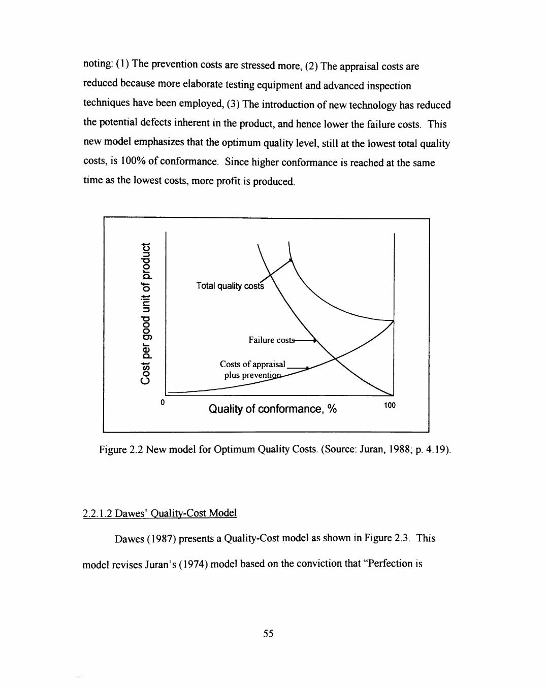
noting: (1) The prevention costs are stressed more, (2) The appraisal costs are
reduced because more elaborate testing equipment and advanced inspection
techniques have been employed, (3) The introduction of new technology has reduced
the potential defects inherent in the product, and hence lower the failure costs. This
new model emphasizes that the optimum quality level, still at the lowest total quality
costs, is 100% of conformance. Since higher conformance is reached at the same
time as the lowest costs, more profit is produced.
o T3 O Q .
» • -O
T3 O O O) v _ (D Q .
V) O
O
Total quality costs
Costs of appraisal plus prevent!
Failure costs
Quality of conformance, % 100
Figure 2.2 New model for Optimum Quality Costs. (Source: Juran, 1988; p. 4.19).
2.2.1.2 Dawes' Quality-Cost Model
Dawes (1987) presents a Quality-Cost model as shown in Figure 2.3. This
model revises Juran's (1974) model based on the conviction that "Perfection is
55
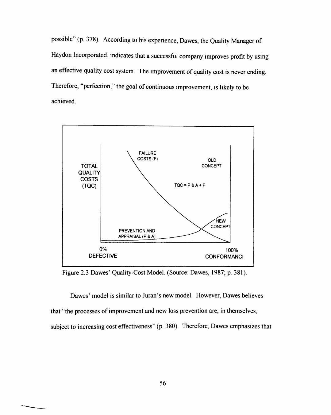
possible" (p. 378). According to his experience, Dawes, the Quality Manager of
Haydon Incorporated, indicates that a successful company improves profit by using
an effective quality cost system. The improvement of quality cost is never ending.
Therefore, "perfection," the goal of continuous improvement, is likely to be
achieved.
TOTAL QUALITY COSTS (TOO
FAILURE COSTS (F) OLD
CONCEPT
TQC = P & A + F
NEW CONCEPTl
PREVENTION AND APPRAISAL (P & A
0% DEFECTIVE
100% CONFORMANCI
Figure 2.3 Dawes' Quality-Cost Model. (Source: Dawes, 1987; p. 381).
Dawes' model is similar to Juran's new model. However, Dawes believes
that "the processes of improvement and new loss prevention are, in themselves,
subject to increasing cost effectiveness" (p. 380). Therefore, Dawes emphasizes that
56
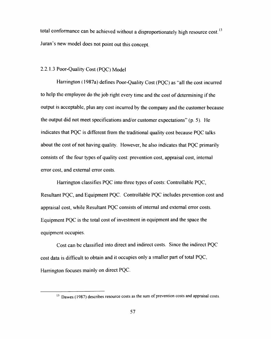
total conformance can be achieved without a disproportionately high resource cost.'"*
Juran's new model does not point out this concept.
2.2.1.3 Poor-Quality Cost (PQC) Model
Harrington (1987a) defines Poor-Quality Cost (PQC) as "all the cost incurred
to help the employee do the job right every time and the cost of determining if the
output is acceptable, plus any cost incurred by the company and the customer because
the output did not meet specifications and/or customer expectations" (p. 5). He
indicates that PQC is different from the traditional quality cost because PQC talks
about the cost of not having quality. However, he also indicates that PQC primarily
consists of the four types of quality cost: prevention cost, appraisal cost, internal
error cost, and external error costs.
Harrington classifies PQC into three types of costs: Controllable PQC,
Resultant PQC, and Equipment PQC. Controllable PQC includes prevention cost and
appraisal cost, while Resultant PQC consists of internal and external error costs.
Equipment PQC is the total cost of investment in equipment and the space the
equipment occupies.
Cost can be classified into direct and indirect costs. Since the indirect PQC
cost data is difficult to obtain and it occupies only a smaller part of total PQC,
Harrington focuses mainly on direct PQC.
' Dawes (1987) describes resource costs as the sum of prevention costs and appraisal costs
57
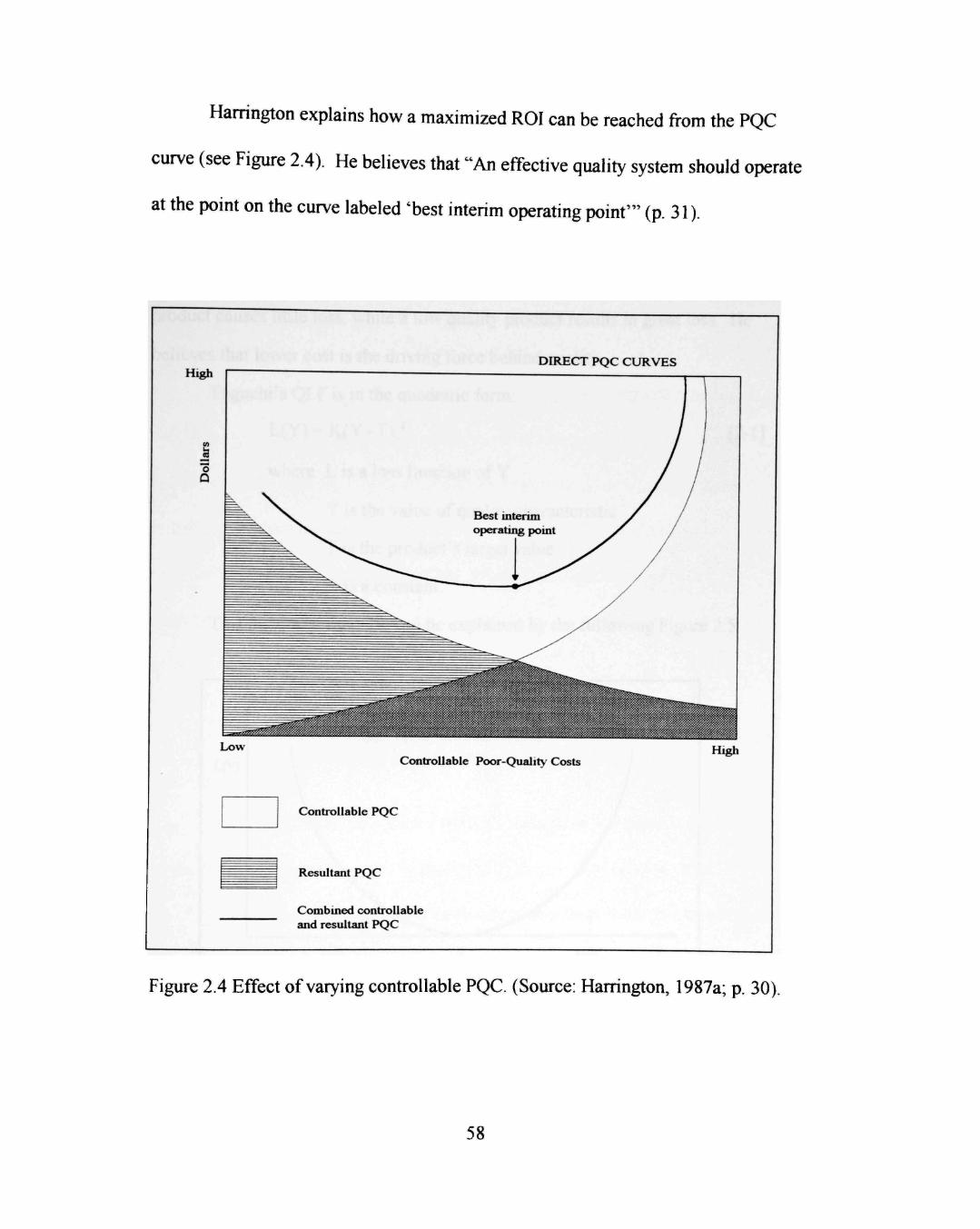
Hamngton explains how a maximized ROI can be reached fi-om the PQC
curve (see Figure 2.4). He believes that "An effective quality system should operate
at the point on the curve labeled 'best interim operating point'" (p. 31).
High DIRECT PQC CURVES
o Q
Lx)w Controllable Poor-Quality Costs
High
Controllable PQC
Resultant PQC
Combined controllable and resultant PQC
Figure 2.4 Effect of varying controllable PQC. (Source: Harrington, 1987a; p. 30).
58
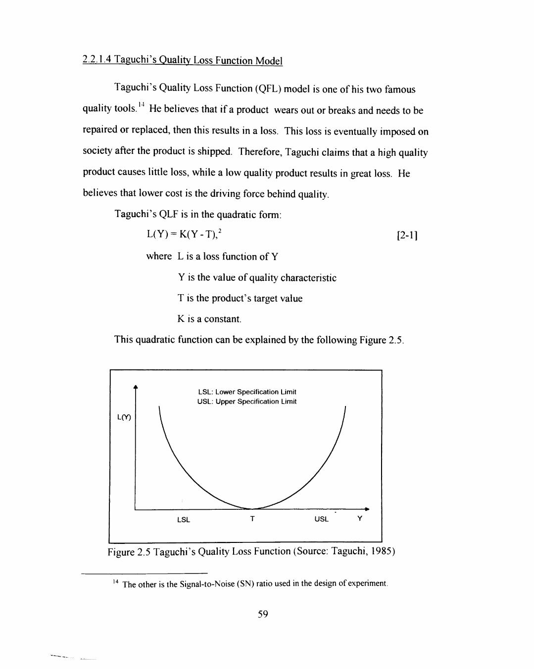
2.2.1.4 Taguchi's Quality Loss Function Model
Taguchi's Quality Loss Function (QFL) model is one of his two famous
quality tools. ' He believes that if a product wears out or breaks and needs to be
repaired or replaced, then this results in a loss. This loss is eventually imposed on
society after the product is shipped. Therefore, Taguchi claims that a high quality
product causes little loss, while a low quality product results in great loss. He
believes that lower cost is the driving force behind quality.
Taguchi's QLF is in the quadratic form:
L(Y) = K(Y-T),' [2-1]
where Lisa loss function of Y
Y is the value of quality characteristic
T is the product's target value
K is a constant.
This quadratic function can be explained by the following Figure 2.5.
i
L(Y)
LSL: Lower Specification Limit USL: Upper Specification Limit v^^
LSL T USL Y
Figure 2.5 Taguchi's Quality Loss Function (Source: Taguchi, 1985)
"* The other is the Signal-to-Noise (SN) ratio used in the design of experiment.
59
In Taguchi's QLF concept, the loss is zero if the target value of the quality
characteristic is exactly at the central limit. In other words, at this point, the profit is
maximized. Therefore, the management should reduce the product's variability as
much as possible in order to maximize profit.
2.2.2 Productivity-Profit Model
As previously stated, no one questions the positive correlation between
productivity and profit, especially when output is measured in terms of dollars.
However, because of the variety ofproductivity measures, no universal model
regarding productivity-profit can be achieved. In this subsection, six productivity-
profit relationship models are addressed: Adam-Hershauer-Ruch's model,
Papadimitriou's Profit Decomposition Model, Sumanth's model, the APC model.
Miller's model, and Miller's ROI-based model..
2.2.2.1 Adam-Hershauer-Ruch's Productivity-Profitability Relationship Model
Adam, Hershauer, and Ruch (1981) explained the relationship between
productivity and profit by defining profitability as a ratio of sales to costs.
First, they define sales as the total output quantities times prices, and costs as
the total of each input quantities times unit costs.
Therefore, profitability is defined as
60
Sales _ Output quantities x prices
Costs Input quantities x unit costs '
Equation [2-1] can be rewritten as
Sales Output quantities Prices 7; = ~i — : X [2-31 Costs Input quantities Unit Costs
Adam, Hershauer, and Ruch view the ratio of'Output quantities' to 'Input
quantities' as 'Productivity'. They also regard the ratio of'Prices' to 'Unit costs' as
'Price Recovery'. Therefore, equation [2-3] becomes equation [2-4], which is
identical to APC Model ( described later).
Profitability = Productivity x Price Recovery [2-4]
2.2.2.2 Papadimitriou's Profit Decomposition Model (PDM)
Papadimitriou (1992) presented the Profit Decomposition Model (PDM). The
derivation of this model is illustrated as follows:
1st step: Papadimitriou defines profit as the difference between total sales
and total costs. This definition can be written in a formula:
^ = PQ-lLPiqi [2-5]
where ;r= Profit
P = Sales price
Q = Volume
61
Pj = The ith Input price
q, = The ith Input quantity
2nd step: By first totally differentiating, equation [2-5] becomes equation [2-
6].
dTT = PdQ + QdP - Y.Pidq. - Y.<iidp, [2-6]
3rd step: Multiplying equation [2-6] by successive terms of one in the form of
d;r=PdQxQ/Q + QdPxP/ P-Yj^,dq. xq, /q, -Yjii^P ""PlP [^'^l
Equation [2-5] can also be rewritten as
P = i [2-8] Q
Replacing equation [2-8] into equation [2-7] yields
d;r = 7dQ/Q+PQdP/ P+Y^Pi^MQIQ-'^t / < )-Y.Piqi^P 'P [2-9]
where ndQ IQ = Volume contribution
PQdP I P = Sales price contribution
YjPi^i ^^0/ Q-^^i l^i)^ Multi-factor productivity contribution /•
Y^PiRi^Pi I Pi ^ ^"P^^ P"^^ contribution.
62
4th step: Papadimitriou believes that in the real environment, discrete data is
frequently used and the changes in data values are large. Therefore, he claims that
the equation [2-9] must be corrected by including interaction terms.
+ APAO-I.Ap.Aq. [2-10]
Equation [2-10] is the basic PDM.
5th step: Dividing equation [2-10] by last period's profit level yields equation
[2-11].
A;r ;rAQ/Q^PQAP/P . ^P'^^^^Q^0-^^'^^'^
;r(-l) 7r{-\) ;r(-l) ;r(-l)
-^ + . [2-11]
7t{-\) 7r{-\) 7r{-\)
Equation [2-11] indicates the percent contribution of each determinant to the
growth in profits.
6th step: The third term of equation [2-10] can be further decomposed into
two components: productivity contribution due to scale and productivity contribution
due to factor prices. That is,
Y,P^qA^QiQ-^q:iqi) = [ Y.qA^QiQ)-^q.iqi ] +
[ ZA'?,(Ae/e'-A?,/?,)-(Z'7,A(?/C?-A^,/</,) 1- [2-12]
63
The terms in the first bracket of the right-hand side of equation [5-11] is the
productivity contribution due to scale, while the first term in the second bracket is the
productivity contribution due to factor prices.
Papadimitriou points out that the decomposition demonstrates an increase of
factor price can offset the decline ofproductivity grov^h. This will resuh in an
increase in profit growth due to productivity. Therefore, Papadimitriou stresses that
"productivity does not have to increase at an increasing rate for the productivity
contribution to profit growth to increase" (p. 63).
2.2.2.3 Sumanth's Productivity-Profit Relationship Model
Sumanth (1979) developed a mathematical relationship model of Total
Productivity and profit. His model is as follows:
Profit P = TP(I) - ( IH + IM + Ic.F + IE + Ix ), [2-13]
where,
TP : Total Productivity
0 O TP = —= - [2-14]
1 IH + IM + IC.F + W + IE + x
where,
O : total tangible output
I: total tangible input
IH : human input
64

IM : material and purchased parts input
Ic F: fixed capital input
Ic,w : working capital input
IH : energy input
Ix : other expense input.
If total output is held constant, then equation [2-14] becomes
P = 0 - ( I H + IM + IC,F + IE + IX), [2-15]
P = 0 - r [2-16]
where, I ' : input costs other than working capital.
Because O is constant, there is a linear negative relationship between I'
and P (see Figure 2.6).
According to equation [2-15] or [2-16], Sumanth's model illustrates the
relationship between Total Productivity and profit: Profit increases as output
increases and/or input decreases.
65
Profits ($)
Profit Curve at q (increased output level)
- Profit Curve at q, (base period output level)
Profit Curve at q, (decreased output level)
Increasing Output
Input Costs Other Than Working Capital
Figure 2.6 The Relationship between Profits and Input Costs. (Source: Sumanth and Wardhana; pp. 463-474).
66

2.2.2.4 APC's Productivity-Profit Relationship Model
American Productivity Center (APC) presented a productivity-profit model in
the early 1980's. This model revised a basic system proposed by Basil Von
Loggerenberg and developed it into a model. The following describes this model:
First, define
Output Value = Quantity Sold x Unit Price, [2-17]
Input Value = Quantity Used x Unit Cost, [2-18]
Output Value o im and Profitability = ^ \^^ ,—, [2-19]
Input Value
Quantity Sold o ^m Productivity = . „ ., [2-^^l
Quantity Used
Unit Price n l^^ Price Recovery = _. .^^ ^ • L - 11
Unit Cost
Then the productivity-profit relationship become:
Profitability = Productivity x Price Recovery. [2-22]
It is obvious that this model shows the positive correlation between
productivity and profit.
2.2.2.5 Miller'^ Productivity-Profit Relationship Model
Miller (1984) also developed a productivity-profit relationship model similar
to APC's model. However, as described in Section 2.1.1.4, Miller's model has two
67
significant points which differ fi-om APC's model. First, Miller's model uses dollar
figures in both profitability, productivity, and price recovery, while APC's model
uses ratios. Second, Miller's model produces cumulative values, whereas the APC's
model considers only period-to-period data when comparing two periods. That is,
APC's model does not take into account the inflation factor or sales prices in the
intervening periods.
Because of these two different points. Miller presented his model in this form:
Profitability = Productivity + Price recovery,^ [2-23]
where
Productivity contribution in period t = (SalesDt) (MarginDt
- Margins), [2-24]
where
SalesDt: the deflated net sales in period t
MarginDt: the deflated gross profit margin in period t
Margins : the profit margin ofthe base period.
Price recovery contribution in period t = (SalesPRt)(MarginPRt
- Margins), [2-25]
where
SalesPRt: the price-generated revenue in period t.
' Note the right side of equation is the sum ofproductivity and price recovery In the APC model, equation [2-22], the right side of equation is a product ofproductivity and price recovery
68

MarginPRt: the price margin that equals the difference
between price-generated revenue and inflation-
generated cost divided by price-generated revenue.
Profit change = actual profit - anticipated profit, [2-26]
or
Profit change in period t = (salest)(margint - margins). [2-27]
Miller's model also illustrates the positive relationship between productivity
and profit.
2.2.2.6 Miller's Productivity-ROI Relationship Model
Miller (1987) believes that "a firm's true criterion of profitability is return on
investment (ROI)" (p. 1051). Thus, he presents a model based on ROI to modify the
profit-linked models.
First, Miller formulates the profitability change P, as
P, = (Sf - O - [ { S ^ -C4)l Ii)]{lf) [2-28]
where S = Net sales
C = Cost
I = Capital Investment
A = Actual dollar amount
B = Base period index
t = time period index.
69
Equation [2-28] can be rewritten into equation [2-29] by multiplying the unit
quantity (.Sg / S'^).
^A r^A p,=i^:-c:)-Mis',{p;ni) [2-29]
.4 ic^A where M'^ = Profit margin = 1- QIS^
Second, equation [2-29] can be refined by partitioning A into price (or
inflation) component (denoted by superscript P) and quantity component (superscript
D). Therefore,
/ = (5,^-cf)+(5;-c;)-M^ 0.4 O.J
ID ' D
[2-30]
£) _ C--1 jD _ jA Third, because at base period 5, = S] , /, = /,
^ . 1 o D
= s? DrrD =srT, [2-31]
where, T,^ = ^ ^ , is the indexed change in deflated or real
S, II,
capital turnover in period t.
Replacing T,^ into equation [2-30], yields equation [2-32].
P. = [ (Si'-Cn-M-iSfT,' ] + [ ( 5 ; - C ; ) - M X / r ] [2-32]
The two terms in the first bracket stands for the productivity component,
while the two terms in the second bracket represents the price recovery component.
70
Fourth, the productivity component can be rewritten by subtracting M^SJ^
fi-om the firs term (Sl" - C,^), and adding M^Sl" to the second term M^SJ'T,''. This
yields equation [2-33].
K=[ {S:'-C^)-MXT^' ] + [ M^Sl^il-T,^) ] [2-33]
where F, is the productivity contribution in period t.
According to Miller (1987), the first term in equation [2-33] is "the same
productivity component as is used in the marginal approach" (p. 1502). He further
indicates that "the growth in ROI can be analyzed in terms of a margin goal for real
or deflated productivity performance, as well as a margin goal for capital investment"
(p. 1502-1503).
2.2.3 Quality-Productivity Relationship Models
In this section, several Quality-Productivity models are addressed. As Garvin
(1988) points out, research on the relationship between quality and productivity are
few, all the models regarding Quality-Productivity relationship are presented. The
most significant model to this research is the Sumanth and Wardhana's Quality-
Profit-Productivity model. This model is the only model that discuss the Quality-
Productivity relationship based on profit. Before Sumanth's model, four models are
first presented. These four models are Adam-Hershauer-Ruch model, Deming's
model, Edosomwan's model, and Thor's model.
71
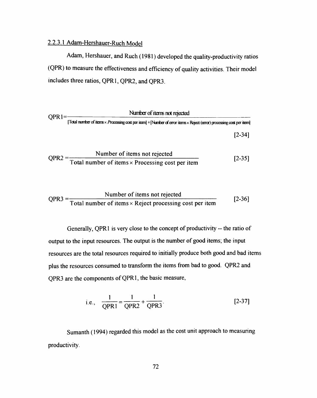
2.2.3.1 Adam-Hershauer-Ruch Model
Adam, Hershauer, and Ruch (1981) developed the quality-productivity ratios
(QPR) to measure the effectiveness and efficiency of quality activities. Their model
includes three ratios, QPRl, QPR2, and QPR3.
^r^^, Nunter of items not idected QPRl^ [Tctel iiinixr of itore X Axx»sii^ cc3St pff ilen^+[Niiite of OTo-it^
[2-34]
^^^ Number of items not rejected OPR2 = —- r'?-' 51
Total number of items x Processing cost per item
Number of items not rejected QPR3 =- : ; ; r - —. : [2-36]
Total number of items x Reject processing cost per item
Generally, QPRl is very close to the concept ofproductivity - the ratio of
output to the input resources. The output is the number of good items; the input
resources are the total resources required to initially produce both good and bad items
plus the resources consumed to transform the items from bad to good. QPR2 and
QPR3 are the components of QPRl, the basic measure.
i e — ^ = — — + • [2-37] ' QPRl QPR2 QPR3
Sumanth (1994) regarded this model as the cost unit approach to measuring
productivity.
72
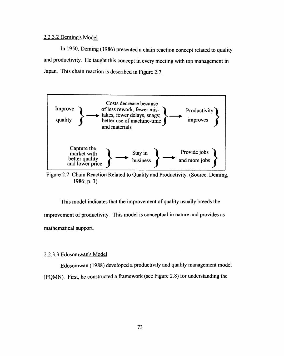
2.2.3.2 Deming's Model
In 1950, Deming (1986) presented a chain reaction concept related to quality
and productivity. He taught this concept in every meeting with top management in
Japan. This chain reaction is described in Figure 2.7.
Improve
quality } Costs decrease because
of less rework, fewer mistakes, fewer delays, snags; better use of machine-time and materials
} Productivity^
improves
Capture the market with
better quality and lower pnce }
Stay in business }
Provide jobs
and more jobs } Figure 2.7 Chain Reaction Related to Quality and Productivity. (Source: Deming,
1986; p. 3)
This model indicates that the improvement of quality usually breeds the
improvement ofproductivity. This model is conceptual in nature and provides as
mathematical support.
2.2.3.3 Edosomwan's Model
Edosomwan (1988) developed a productivity and quality management model
(PQMN). First, he constructed a framework (see Figure 2.8) for understanding the
73
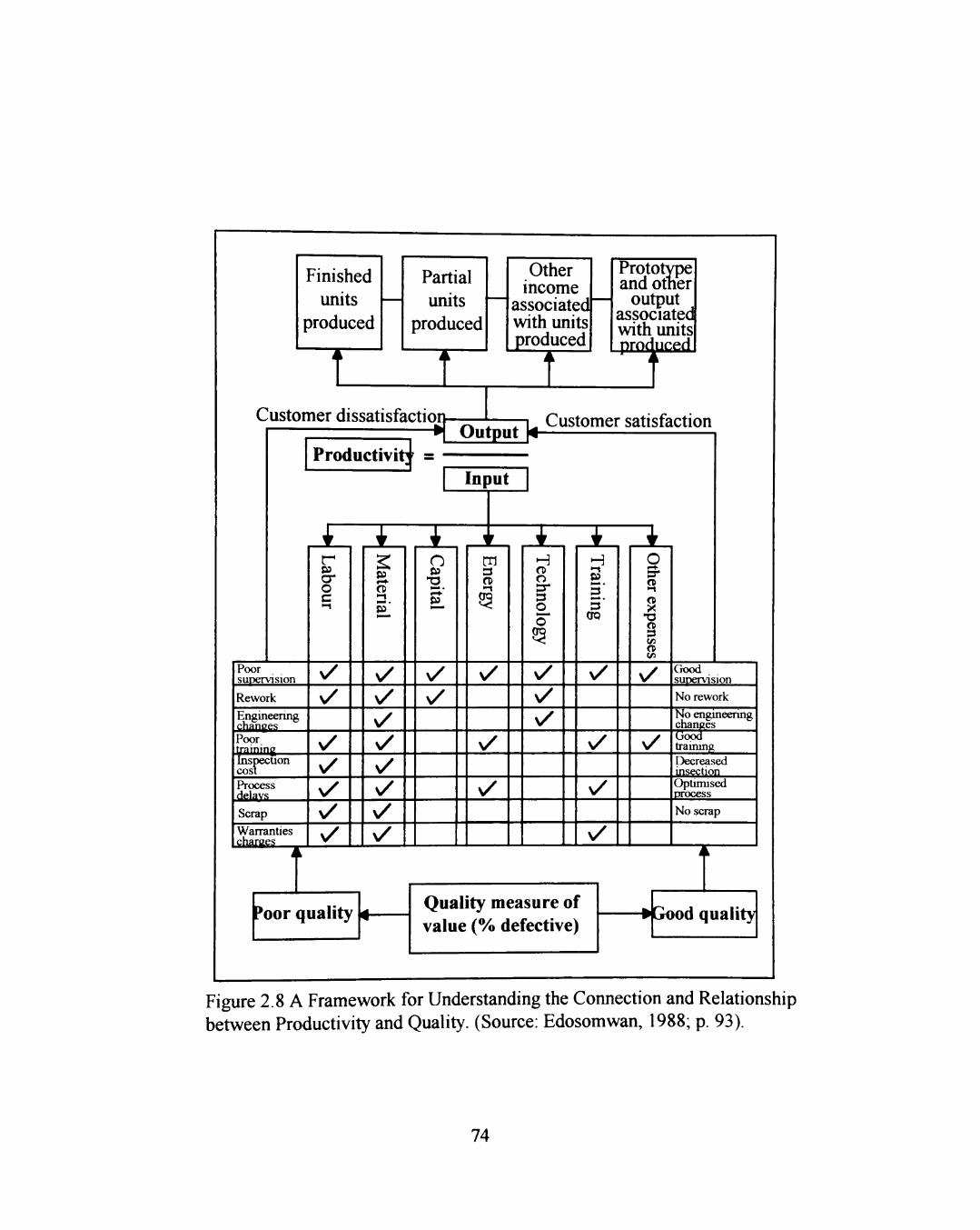
Finished units
produced
I
Partial units
produced
I
Other income
associated with units produced
Customer dissatisfactio
I
Prototype and other
output associated with units pro4uced produ
Productivity =
n 1 H Output
Customer satisfaction
Input
Poor supervision
Rework
Engineering changgs Poor training Inspection cost spect
St Process delays Scrap
Warranties charges
£ r cr o c •-t
N /
N /
v/ s / N /
v/ ^/
I c\>
s/
y v/ v / v / v / x/ v /
I n p
v/ N /
3 CD •-I
v/
x /
N /
H a o 3 o
e?
s/ > /
x /
I H •-I
5' 5'
OQ
N /
v/
v /
x /
cr l-l
X o 1/3
C/3
v/
v /
Good supervision
No rework
No engineering changes cnange Uopd training Decreased insection Optimised t?rocess
No scrap
E oor quality # Quality measure of value (% defective) #(jOod quality
Figure 2.8 A Framework for Understanding the Connection and Relationship between Productivity and Quality. (Source: Edosomwan, 1988; p. 93).
74
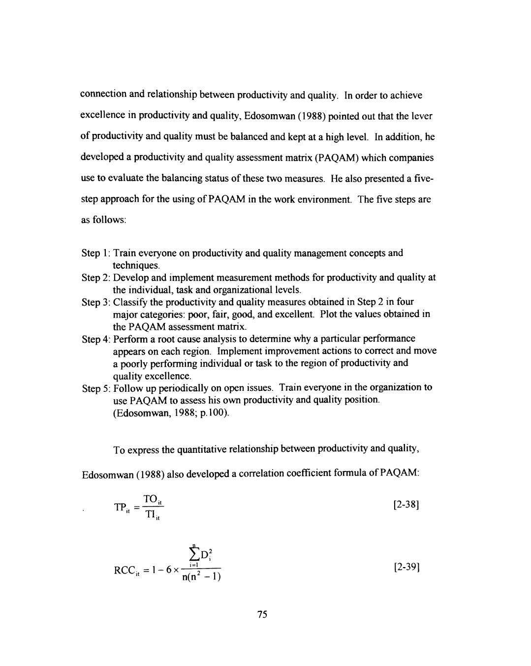
connection and relationship between productivity and quality. In order to achieve
excellence in productivity and quality, Edosomwan (1988) pointed out that the lever
of productivity and quality must be balanced and kept at a high level. In addition, he
developed a productivity and quality assessment matrix (PAQAM) which companies
use to evaluate the balancing status of these two measures. He also presented a five-
step approach for the using of PAQAM in the work environment. The five steps are
as follows:
Step 1: Train everyone on productivity and quality management concepts and techniques.
Step 2: Develop and implement measurement methods for productivity and quality at the individual, task and organizational levels.
Step 3: Classify the productivity and quality measures obtained in Step 2 in four major categories: poor, fair, good, and excellent. Plot the values obtained in the PAQAM assessment matrix.
Step 4: Perform a root cause analysis to determine why a particular performance appears on each region. Implement improvement actions to correct and move a poorly performing individual or task to the region ofproductivity and quality excellence.
Step 5: Follow up periodically on open issues. Train everyone in the organization to use PAQAM to assess his ovm productivity and quality position. (Edosomwan, 1988; p. 100).
To express the quantitative relationship between productivity and quality,
Edosomwan (1988) also developed a correlation coefficient formula of PAQAM:
TO TP, = - ^ ^ [2-38]
ID; n ( n ^ - l )
RCC, = l - 6 x - f V - T : [2-391
75
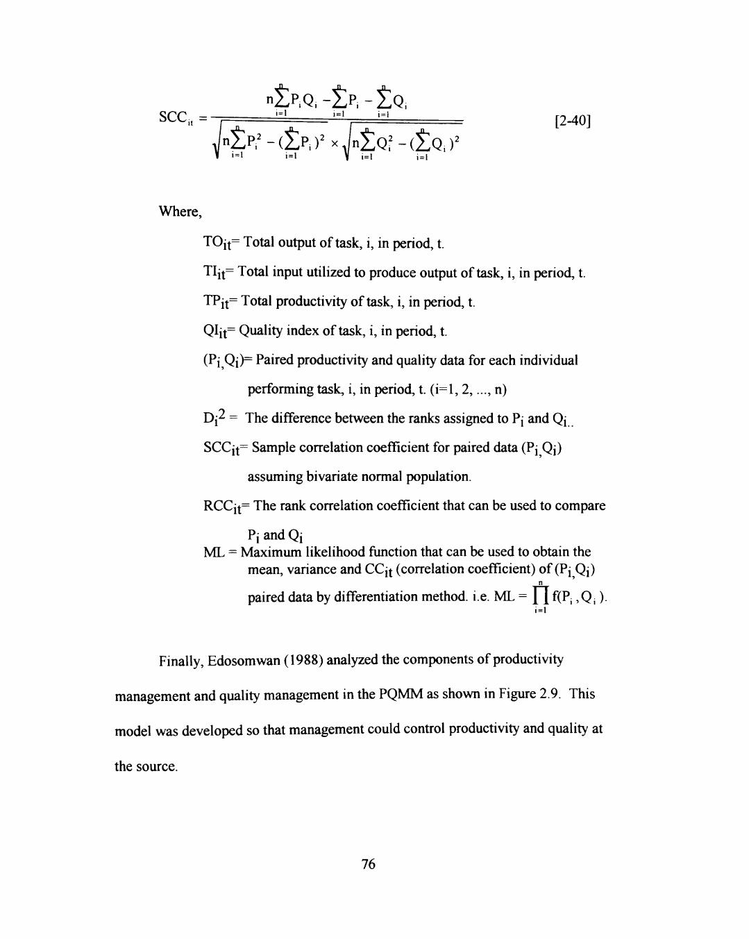
[2-40] sec. = ^ L '-' '-' Jr^lP- -(IP.Y Jn^Q^ -(±Q,y V 1 = 1 i = l V i = l i = l
Where,
TOit= Total output of task, i, in period, t.
Tl{f= Total input utilized to produce output of task, i, in period, t.
TP{f= Total productivity of task, i, in period, t.
QIit= Quality index of task, i, in period, t.
(Pi Qi)= Paired productivity and quality data for each individual
performing task, i, in period, t. (i=l, 2,..., n)
Di2 = The difference between the ranks assigned to P{ and Q{
SCCit= Sample correlation coefficient for paired data (P Qj)
assuming bivariate normal population.
RCCit= The rank correlation coefficient that can be used to compare
Pj and Qi ML = Maximum likelihood function that can be used to obtain the
mean, variance and CCit (correlation coefficient) of (Pi Qi) n
paired data by differentiation method, i.e. ML = J j f(Pi ,Q,). i = i
Finally, Edosomwan (1988) analyzed the components ofproductivity
management and quality management in the PQMM as shown in Figure 2.9. This
model was developed so that management could control productivity and quality at
the source.
76
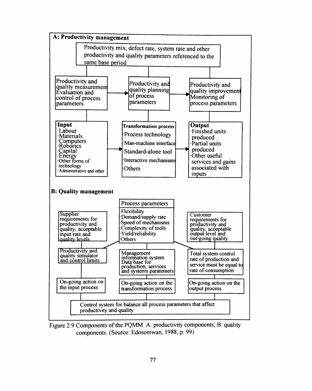
A: Productivity management
Productivity mix, defect rate, system rate and other productivity and quality parameters referenced to the same base period
Productivity and quality measuremen Evaluation and control of process parameters
Input •Labour •Materials •Computers •Roborics •Capital •Energy •Other forms of technology 'Administrative and other
B: Quality management
Supplier requirements for productivity and quality, acceptable input rate and qualify leyek
Productivity and quality simulator and control limits
On-going action on the input process
Productivity anc quality planning of process parameters
Transformation process
Process technology
Man-machine interface
Standard-alone tool
Interactive mechanism'
Others
Process parameters •Flexibility •Demand/supply rate •Speed of mechanisms •Complexity of tools •Yield/reliability •Others
Management information system Data base for production, services and systems paratemers
I On-going action on the transformation process
Productivity and quality improvemen Monitoring of process parameters
Output •Finished units produced •Partial units produced •Other useful services and gains associated with inputs
Customer requirements for productivity and quality, acceptable output level and out-going quality t Total system control rate of production and service must be equal to rate of consumption
On-going action on the output process
Control system for balance all process parameters that affect productivity and quality
Figure 2.9 Components ofthe PQMM. A: productivity components; B: quality components. (Source: Edosomwan, 1988; p. 99)
77
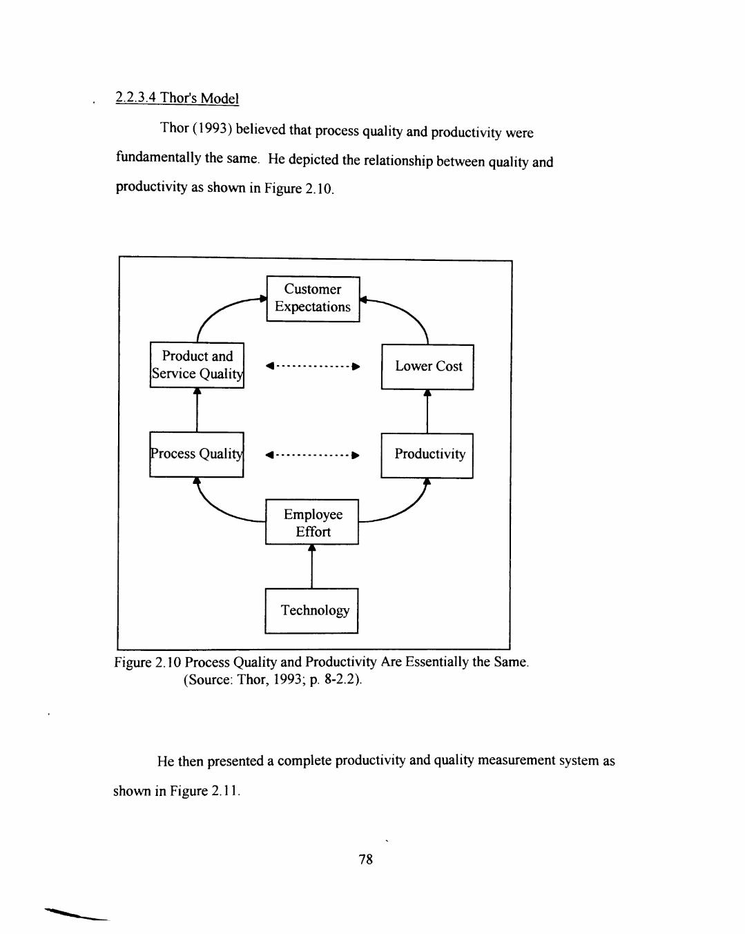
2.2.3.4 Thor's Model
Thor (1993) believed that process quality and productivity were
fundamentally the same. He depicted the relationship between quality and
productivity as shown in Figure 2.10.
Product and Service Quality
i i
Process Quality
Customer Expectations
< •
^ . . . . . . . . . . . . . . ^ ^ . . . . . . . . . . . . . . ^
Employee Effort
Technology
Lower Cost
ii
Productivity
Figure 2.10 Process Quality and Productivity Are Essentially the Same. (Source: Thor, 1993; p. 8-2.2).
He then presented a complete productivity and quality measurement system as
shown in Figure 2.11.
78
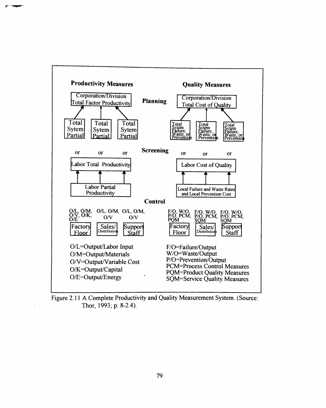
Productivity Measures
Corporation/Division Total Factor Productivity
7 Total Sytem Partial
Total Sytem Partial
X Planning
Total Sytem Partial
or or or Screening
Labor Total Productivity
Labor Partial Productivity
Control
Quality Measures
Corporation/Division Total Cost of Quality
lure, (aste, or
^reventio i
X [otal >vtem lilure,
./aste, or 'reventioi i
or or or
Labor Cost of Quality
Local Failure and Waste Rates and Local Prevention Cost
0/L, 0/M, 0/V, 0/K, 0/E
0/L, 0/M, 0/L, 0/M, O/V 0/V
Factory Floor
Sales/ Distribulioi i
Suppor Staff
W^W9i F/0,W/0, F/0,W/0, P/0 PCM, P/0 PC\i P/0 PCM, PQM SQM SQM Factory Floor
Sales/ Distributioh
Suppor Staff
0/L=Output/Labor Input 0/M=Output/Materials 0/V=Output/Variable Cost 0/K=Output/Capital 0/E=Output/Energy
F/0=Failure/Output W/0=Waste/Output P/0=Prevention/Output PCM=Process Control Measures PQM=Product Quality Measures SQM=Service Quality Measures
Figure 2.11 A Complete Productivity and Quality Measurement System. (Source: Thor, 1993; p. 8-2.4).
79
2.2.3.5 Sumanth and Wardhana s Quality-Profit-Productivity (OPP) Relationship Model
Sumanth and Wardhana (1993) developed a mathematical relationship model
between Quality of Conformance, Profit, and Total Productivity (QPP). This model
is based on the Dawes' model and Sumanth's total productivity model, break-even
point of total productivity, and productivity-oriented profit. This model measures the
quality-profit relation through the interaction with total productivity.
By using this model, the effects of a changed output on the total productivity
and profit can be measured at a fixed level of quality of conformance.
The QPP model is developed as follows:
1. Develop a mathematical relationship between total productivity and profit.
This model, developed by Sumanth (1979), has been stated in subsection
2.2.2.1.
2. Divide each inputs of TP into five parts:
a. The portion ofthe input not directly related to the quality system (nq).
b. The portion ofthe input not directly related to appraisal cost (a).
c. The portion ofthe input not directly related to prevention cost (p).
d. The portion ofthe input not directly related to internal failure cost (if).
e. The portion ofthe input not directly related to external failure cost (ef).
Then,
80
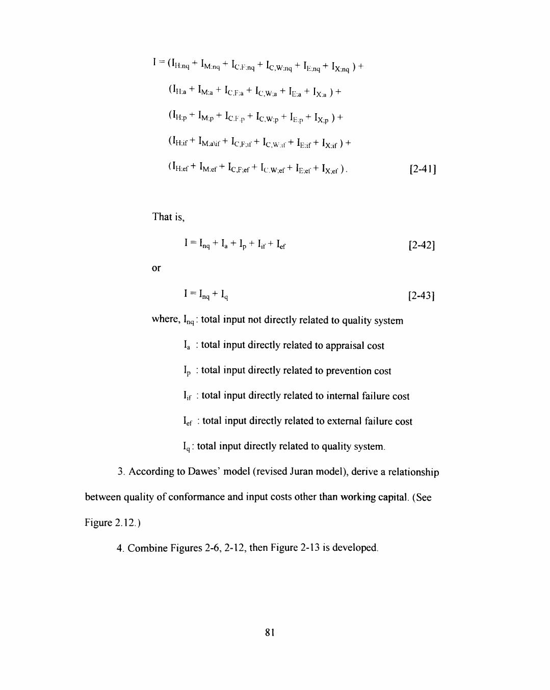
J = (lH:nq + Iw.nq + Ic.F.nq + Ic,W:nq + Il-nq + Ix;nq ) +
(lH:a + lM:a + Ic,F.a + Ic,W:a + k:. + Ix:a ) +
( I H . P + IM;P + Ic .Fp + Ic,W;p + Ic.p + Ix;p ) +
( W + lM.a\ir+ Ic,F;,f+ Ic,W:,f + lE:if + Ix:if ) +
(iH.ef + iM.ef + IcJ^;ef + Ic.W;ef + lE.ef + Ix;er ) • [ 2 - 4 1 ]
That is,
l = I n q + I a + I p + I . r + I e f [ 2 - 4 2 ]
or
I = Inq + Iq [2-43]
where, Inq: total input not directly related to quality system
la : total input directly related to appraisal cost
Ip : total input directly related to prevention cost
I,f : total input directly related to internal failure cost
lef : total input directly related to external failure cost
Iq: total input directly related to quality system.
3. According to Dawes' model (revised Juran model), derive a relationship
between quality of conformance and input costs other than working capital. (See
Figure 2.12.)
4. Combine Figures 2-6, 2-12, then Figure 2-13 is developed.
81
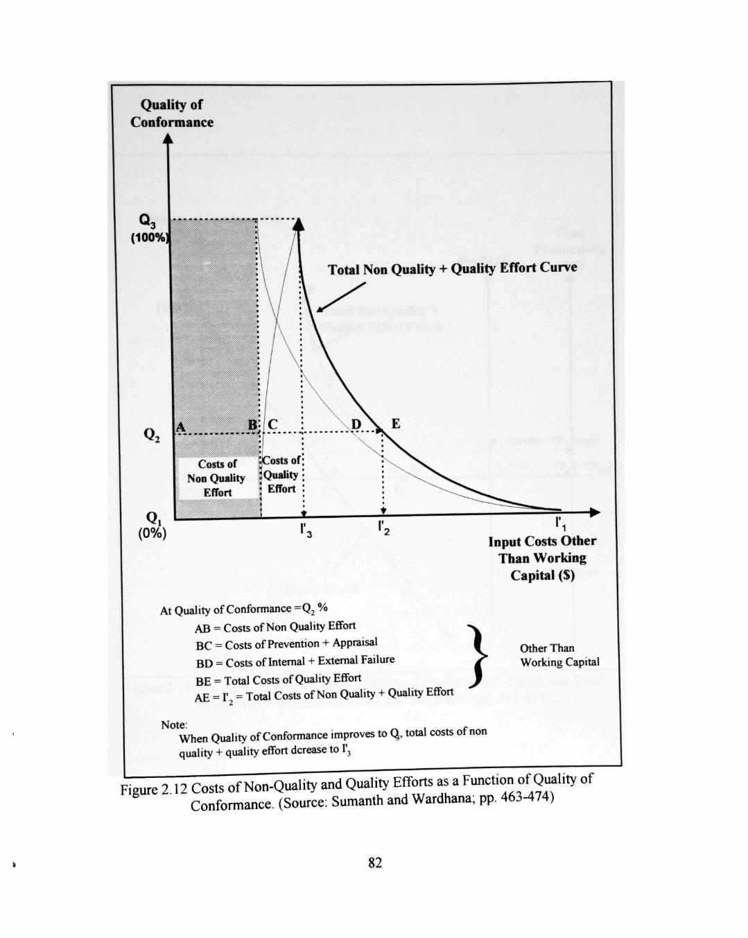
Quality of Conformance
•
(100%
Total Non QuaUty + Quality Effort Curve
Input Costs Other Than Working
Capital ($)
At Quality of Conformance =Q2 %
AB = Costs of Non Quality Effort
BC = Costs of Prevention + Appraisal
BD = Costs of Internal + External Failure
BE = Total Costs of Quality Effort AE = r = Total Costs of Non Quality + Quality Effort
Other Than Working Capital
Note When Quality of Conformance improves to Q, total costs of non quality + quality effort dcrease to F,
Figure 2 12 Costs of Non-Quality and Quality Efforts as a F^^^ion of Quality of Conformance. (Source: Sumanth and Wardhana; pp. 463-474)
82
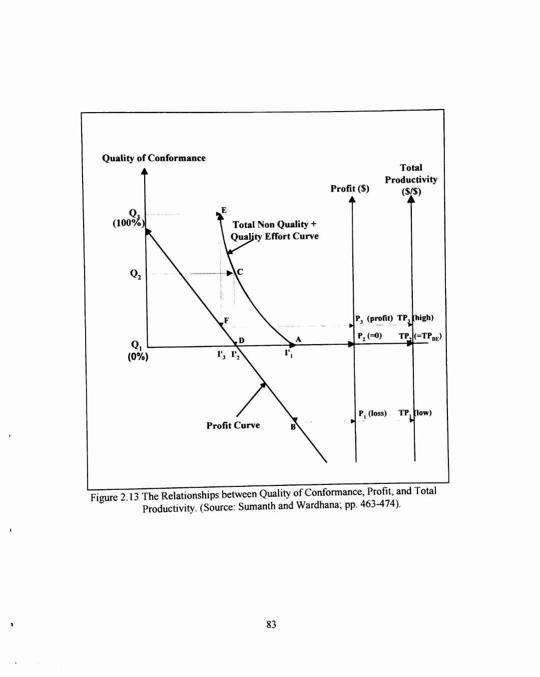
Quality of Conformance A
(100%)
Q,
(0%)
Profit ($)
Total Non Quality + ty Effort Curve
Profit Curve
Total Productivity
( $ / $ )
P3 (profit) TP
P, (=0) TP.
high)
(=TPBE)
P, (loss) TP low)
Figure 2 13 The Relationships between Quality of Conformance, Profit, and Total Productivity. (Source: Sumanth and Wardhana; pp. 463-474).
83
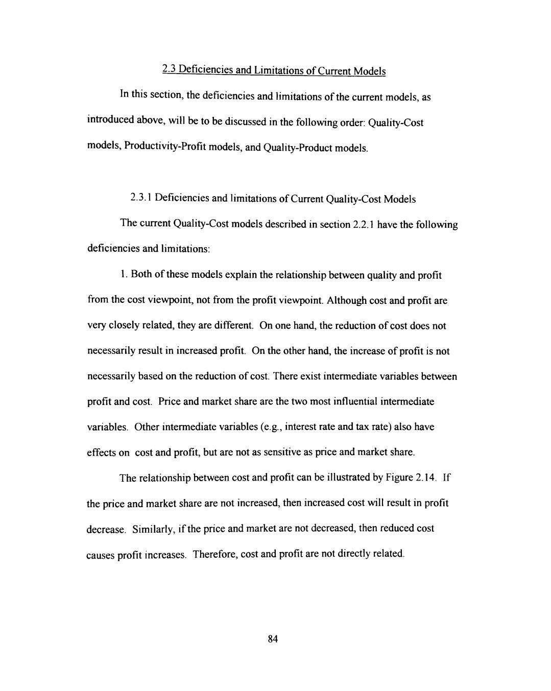
2.3 Deficiencies and Limitations of Current Models
In this section, the deficiencies and limitations ofthe current models, as
introduced above, will be to be discussed in the following order: Quality-Cost
models, Productivity-Profit models, and Quality-Product models.
2.3.1 Deficiencies and limitations of Current Quality-Cost Models
The current Quality-Cost models described in section 2.2.1 have the following
deficiencies and limitations:
1. Both of these models explain the relationship between quality and profit
from the cost viewpoint, not from the profit viewpoint. Although cost and profit are
very closely related, they are different. On one hand, the reduction of cost does not
necessarily result in increased profit. On the other hand, the increase of profit is not
necessarily based on the reduction of cost. There exist intermediate variables between
profit and cost. Price and market share are the two most influential intermediate
variables. Other intermediate variables (e.g., interest rate and tax rate) also have
effects on cost and profit, but are not as sensitive as price and market share.
The relationship between cost and profit can be illustrated by Figure 2.14. If
the price and market share are not increased, then increased cost will result in profit
decrease. Similarly, if the price and market are not decreased, then reduced cost
causes profit increases. Therefore, cost and profit are not directly related.
84
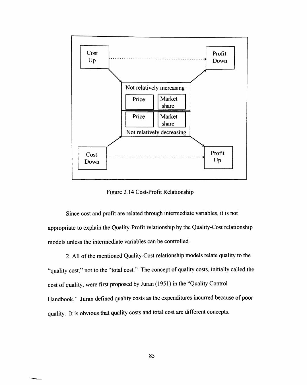
Cost Up
Cost Doyvn
\
Not relatively
Price
Price
increasing
Market share
Market share
Not relatively decreasing •
/
Profit Down
Profit Up
Figure 2.14 Cost-Profit Relationship
Since cost and profit are related through intermediate variables, it is not
appropriate to explain the Quality-Profit relationship by the Quality-Cost relationship
models unless the intermediate variables can be controlled.
2. All ofthe mentioned Quality-Cost relationship models relate quality to the
"quality cost," not to the "total cost." The concept of quality costs, initially called the
cost of quality, were first proposed by Juran (1951) in the "Quality Control
Handbook." Juran defined quality costs as the expenditures incurred because of poor
quality. It is obvious that quality costs and total cost are different concepts.
85
Profit IS produced by subtracting the total costs, not quality costs.
Furthermore, the current quality-cost relationship models determine the optimum
quality level fi-om the total quality costs viewpoint, not from the perspective of total
costs. Therefore, it is inappropriate to measure profit fi-om the quality-cost models
described previously.
3. The revised quality-cost relationship models, either by Juran or Dawes, all
indicate that the optimum quality levels are obtained at the lowest total quality costs.
This assertion is also doubtful.
First of all, their assertion is simply an ideal conceptualization. There is no
mathematical proof or practical evidence to support the notions indicated in the
models. In addition, since Juran and Dawes believe that the optimum quality level is
100% conformance, no defect is allowed. One ofthe reasons that the statistical
method is v^dely applied is that it can save time and costs in guaranteeing a product
reaches a certain quality level, but not 100 % conformance. No one can ensure 100%
conformance quality level with no risk. Under 100% confidence level, the confidence
interval of quality level must be between negative and positive infinity. This interval
is meaningless to management. Therefore, the quality-cost relationship model is just
an ideal model used to arouse the management examining the product quality issue.
4. Taguchi's loss function stresses that the loss incurred by poor quality will
eventually be imposed on society. This is an excellent concept in emphasizing the
importance of good quality; however, it cannot help a company to evaluate the degree
86
of loss incurred by poor product quality. Since the loss will be shared by all of
society, it is not a loss to a single company only. Therefore, the loss function is not a
measurable tool for companies to measure the loss caused by the poor quality.
2.3.2 Deficiencies and limitations of Current Productivity-Profit Models
The deficiencies and limitations ofthe Productivity-Profit Models introduced
in section 2.2.2 are summarized in the following.
1. The Adam-Hershauer-Ruch's model and the APC's model both measure
productivity in terms of quantity/quantity. This unit of measure is not consistent for
all the factors of input or output. For example, labor is one ofthe input factors and is
usually measured in terms of time consumed. Materials are also an input factor but
are meeisured in piece or money. Unless these two factors are being transferred in
terms of costs, they cannot be added together. Therefore, their models cannot
effectively be used in practical application.
Although the Adam-Hershauer-Ruch's model and the APC's model are
identical, they are interpreted differently. The Adam-Hershauer-Ruch's model
interprets productivity by the ratio of output quantity to input quantity, while the
APC's model explains productivity as a ratio of quantity sold to quantity used. The
former model implies that all the output produced can be sold wdthout difficulty in
the market. It seems not to take into account the market's response. On the other
87
hand, the APC's model considers the output from a sales standpoint, it also has
deficiencies, (described in section 2.1.1.4 and 2.2.2, pointed out by Miller (1984)).
2. Sumanth (1979) defined Total Productivity as the ratio of total tangible
output to the sum of all the tangible inputs, as mentioned in Table 2.1 of section
2.1.2.1. Hence, his Productivity-Profit model initially considered "all the inherently
measurable inputs and outputs" (p. 6.3), either in physical terms or in terms of value.
However, as modified later in 1994 by himself, "the tangible output and tangible
input have to be expressed in value terms because all the output and input elements
are not in the same units" (p. 154). His idea is exactly the same as explained in the
first point of this section.
In addition, Sumanth's model has a significant limitation. That is, only the
total tangible output is assumed constant can the negative linear relationship exist
(see section 2.2.2.3). This assumption may be reasonable for a short period of time;
however, from a long-term standpoint, it may not be appropriate. Therefore,
Sumanth's model may not be applicable in the long term.
3. Miller's first model stresses the use of dollars as the unit of measure of
both profitability, productivity, and price recovery. Thus, his model demonstrates
that profitability equals the sum ofproductivity and price recovery, not the product of
productivity and price recovery as expressed by the Adam-Hershauer-Ruch's model
or APC's model.
88
It is unusual that this model expresses both profitability and productivity in
terms of dollars. Since the definitions ofproductivity and profitability examined in
section 2.1.2.1 (Table 2.1) and section 2.1.2.3 (Table 2.3), all show that these two
terms are ratios, the units of measure in the Miller's first model are apparently
different from others and are not easily accepted.
Miller's second model, the Productivity-ROI model, also has the same units of
measure as defined in his first model. He measures the profitability change Pt
(equation [2-28]), and productivity component (the two terms in the first bracket of
equation [2-32]) both in terms of dollars. This also results in the same problem: the
definitions ofproductivity and profitability differ significantly fi-om those generally
accepted.
4. Papadimitriou (1992) explained the Productivity-Profit relationship by the
decomposition approach. He related productivity with the growth of profit.
However, he did not clearly define profitability and the growth of profit. There was
no clear distinction between these two terms.
Based on the above discussion, no current model is perfect. This is to be
expected the models do not have a common definition ofproductivity. Because of
the variety of manufacturing environments, an applicable model must have its own
definitions to develop.
89
2.3.3 Deficiencies and Limitations of Current Quality-Productivity Models
In this section, the deficiencies and limitations ofthe five models presented in
section 2.2.3 are addressed.
1. In Deming's model, he did not give definitions for quality and productivity.
As Deming (1986) stated that "Quality can be defined only in terms ofthe agent" (p.
168), he thought quality had different meanings to different levels of employees.
Deming developed his model to stress his viewpoints that focusing on quality
improvement could lead the productivity improvement. However, because of a lack
of definitions, the relationship between quality and productivity becomes
questionable.
2. Thor's model regards quality and productivity essentially as the same thing.
However, if quality and productivity were the same, then there is no need to discuss
the relationship between them. Since the original meaning of "productivity" is not
used as an another form of "quality," one needs to be carefiil when interpreting the
relationship between these two terms. Quality and productivity are closely related;
however, the degree of relationship may vary in different departments or functions.
Therefore, it is not appropriate to assert that these two terms are synonymous in every
situation.
3. In Adam-Hershauer-Ruch model, the relationship between quality and
productivity from the standpoint ofthe cost unit is considered. Thus, Sumanth (1994)
called it the cost unit approach. He mentions three points to consider on this model:
90
a. The Quality-productivity ratio might be a misleading measure
when the unit processing cost and the unit reject-correction cost
depend on the number of rejected items.
b. The estimated cost based on the historical data might not reflect
the current cost.
c. This model did not show whether or not the rejected goods are
repaired and become acceptable in the same period.
In addition to Sumanth's comments, there are four more issues to be
addressed:
a. It is not clear whether the rejected goods are from the customer's
standpoint or from the standpoint of supplier's quality personnel. Unless
100% inspected, there exists a risk in acceptance sampling between
customer and supplier. Besides, due to the potential difference in the
recognition on product quality, the goods that supplier values may be
determined as rejected by the customer. It will cause some trouble in
determining the number of items not rejected in this model.
b. It does not consider the items not finished. Usually, a specific period of
time is a common base for the calculation of this model; however, during
this time period, it is very likely that some items are not completely
91

finished, i.e., some items remained in work-in-process condition. This
model does not explain how to deal with these work-in-process items,
c. If the unit reject processing cost significantly decreases as the number of
rejected items increases, the QPR may increases even though the percent
defective of items increases. Two cases in Table 2.4 can be used to explain
this fact. Case I is the example used by Adam, Hershauer, and Ruch for
explaining the calculation of QPR. The data of total number of items, unit
processing cost, number of rejected items, and unit reject processing cost in
Case I are given. The QPR value is obtained from equation 2.34. Case 2
assumes that the number of rejected items doubles while the total number
of items and its unit processing cost remain unchanged. The unit reject
processing cost decreases significantly because ofthe increasing number of
rejected items. The QPR increases from 4.5 in case I to 5.0 in case 2. It
demonstrates that the QPR increases, but the percent of good items
decrease. It is easy to understand that the product quality increases while
the number of rejected items is cut in half
Table 2.4 Comparison of QPR Values When Unit Reject Processing Cost Significantly Decreases
Case I
Case 2
Total number of items Nimiber
100
100
Unit processing cost
$0.1
$0.1
Rejected items Number
10
20
Unit rejected processing cost
$1.0
$0.3
QPR
4.5
5.0
92
4. Edosomwan's model considers the quality-productivity relationship from a
broader viewpoint. It presents not only the improvement approach of management,
but also the statistical method in relating the quality-productivity relationship. It is a
more thorough and detailed model than any other. However, it is also necessary to
note some points:
a. The (Pj, Q\) data can be either assigned rank data or measured
quantitative data. Assigned rank data are used for calculating the
rank correlation coefficient RC{C{. RCjCj is used in the PAQAM,
which is a matrix with the ranks of quality and productivity as its
axes. Measured quantitative data are used for calculating the
sample correlation coefficient SCjCj. SCjCj formula assumes
bivariate normal population for paired data {?{, Q[). However,
there is no connection between RCjCj and SCjCi.
b. Sample correlation coefficient SCjC^ expresses the extent and
direction that quality and productivity are correlated. It can also tell
how much variation of one variable is caused by the other variable
based on the coefficient of determination SCjC^ j . However, it
cannot indicate which is the cause and which is the effect. To
discern cause and effect is an important measure for management.
5. Sumanth and Wardhana's QPP model was developed based on Sumanth's
(1979) Total Productivity model and Dawes' model. Therefore, the deficiencies and
93
limitations of these two models mentioned previously still apply to Sumanth and
Wardhana's QPP model. That is:
a. Sumanth and Wardhana's QPP model also employs the quality costs
concept to measure the costs other than working capital.
b. The Sumanth and Wardhana's QPP model may not be applicable for
long-term purposes.
In addition, Sumanth and Wardhana's QPP model also has the following
deficiencies and limitations:
c. This model is used only for quality in terms of level of conformance
( % ) .
d. It is difficult to directly determine the relationship between quality.
Total Productivity, and profit from the two-dimensional Figure 2.13.
e. Based on Figure 2.13, it seems that the quality conformance level at the
break-even-point is always at Q2 = 50% or so. However, this is not
true. As Sumanth and Wardhana described, the quality conformance
level at the break-even-point should at the point where the input costs
other than working capital (F) equals the tangible output at the base
period.
94
2.4 Research Agenda
In this section, definitions regarding the research problem will first be given.
The conceptual model of this research is also presented. These definitions and
conceptual model comprise the basic framework for this research.
2.4.1 Definitions of This Research
Before starting research, it is necessary to clarify the terms used. The
following subsections define and explain the basic terms used in this research:
quality, productivity, profit.
2.4.1.1 Definition of Quality
The term "quality" used in this research refers to the "product quality," or "lot
quality." Product quality is defined as the conformance level ofthe characteristic(s)
of a product that meets customer's specification(s). The point at which the
conformance level just meets the customer's specifications for a product is called the
minimum acceptable product quality.
Because the conformance level can be explained either in terms of individual
product or in terms of lot, product quality as defined above is apparently in terms of
individual product. If a lot conformance level is required, it is called lot quality. Lot
quality is defined as the conformance level at which a lot satisfies the customer
requirement. Similarly, the point at which the conformance level just meets the
95
customer's specified requirement for a lot is called the minimum acceptable lot
quality.
Lot quality is usually specified when 100% inspection is impossible (e.g.,
destructive inspection) or uneconomical. In such situations, sampling inspection is
the only choice. However, because ofthe sampling risk, the customer must allow for
a defined level of defective product.
For example, if ten thousand fluorescent lamps are ordered, it is impossible to
test the product characteristic, (e.g., lighting duration for 1000 hours), for all ten
thousand lamps. In this case, sampling inspection is inevitably applied and a lot
quality (e.g., 99.5% ofthe ten thousand lamps exceed the duration 1000 hours) must
be specified. The minimum acceptable lot quality is 99.5% in this case.
2.4.1.2 Definition of Productivity
In this research, productivity is defined as the profit-based ratio of valuable
output to measurable input during a specified period. The term "valuable outpuf
means that the output has a market value. Also, "measurable input" refers to all the
input that can be measured by or transferred into dollars. Therefore, the unit of
measure for productivity used in this research is dollars to dollars, and productivity is
profit-based.
Because ofthe influence of inflation or deflation, the same amount of dollars
has different values at different times. Since the output always lags behind the input.
96
it is necessary to take into account the inflation or deflation factors. For the purpose
of measuring the productivity of a product, three assumptions are needed here. First,
the time lags between the output and input ofthe same product are assumed constant.
Second, the influence ofthe time lags among input costs are negligible. That is, the
input costs incurred at different time points within a short period of time are assumed
having no deflation of inflation. Third, the influence ofthe time lags among the
outputs sold are negligible. That is, the output (resulted from the same input) values
produced at different time are assumed having no deflation or inflation.
Because the object of this research focuses on manufacturing companies,
valuable output refers to the products that are to be sold to customers, either external
or internal customers. "External customers" are the customers who directly purchase
the products outside the manufacturing company.' "Internal customer" refers to the
other divisions, departments, etc. that are users of valuable products in the same
manufacturing company. On the other hand, input is usually viewed as synonymous
with total cost in the manufacturing environment.
' This definition differs fi-om Juran and Gryna's (1993) definition. They explain the external customers as both ultimate and intermediate users, including government regulatory bodies.
' This definition also diflfers fi-om Juran and (jiyna's (1993) definition. In their explanation, internal customers include all the divisions provided with or affected by components or subassemblies. According to Juran and Gryna, a Purchasing Department is an internal customer because it receives the specifications for procurement. However, a Purchasing Department is not regarded as an internal customer in this research unless it is also a user ofthe manufactured products.
97
In addition, productivity, as defined above, implies the Total Productivity
only. Total Productivity, as defined by Sumanth (1994), is a ratio of total tangible
output to total tangible input. It is a ratio measuring the overall productivity.
2.4.1.3 Definition of Profit
In this research, profit is used as the base to link productivity and quality.
Profit is defined as the difference between revenue and cost.
In addition to the definition, there are three points that need to be noted:
1. In this research, profit refers to the gross profit before tax.
Since different tax rates influence the net profit, and hence may change the
relationships among quality, productivity, and profit, only the profit before
tax is considered.
2. All profits, revenues, and costs are measured in the base-period equivalent
value.
The purpose of this requirement is to rule out the impact caused by
inflation or deflation in the relationship models.
3. Profit comes mainly from the sales of product.
In order to avoid misconstruing the relationships among quality,
productivity, and profit, profits that are not from the sales of product are
not considered in this research.
98

2.4.1.4 Definition of Cost
Cost and profit are closely related. Although in this research, the Quality-
Productivity relationship is developed based on profit, it does relate to the calculation
of cost. Therefore, cost must also be defined for this research.
Except where specified, cost in this research is defined as the production cost.
Since this research focuses on the quality-productivity relationship, the costs incurred
in the production activities are the main concern. The marketing costs and
administrative costs are not included in the production cost.
Production costs include the direct material, direct labor, and factory
overhead incurred to produce a product. Direct material cost is the cost of any raw
material that becomes an identifiable part ofthe finished product. Direct labor cost is
the wage earned by a worker who transforms the state of material or part to another
state, e.g., finished product. Factory overhead includes all production costs other
than direct material and direct labor. Since cost is referred to production cost, factory
overhead is simply called overhead in this research.
Both profit and cost are measured in terms of US dollars in the base period.
Profit and cost in the confirmatory study are converted from Taiwaness currency
values into the equivalent US dollars based on a fixed exchange rate.
99
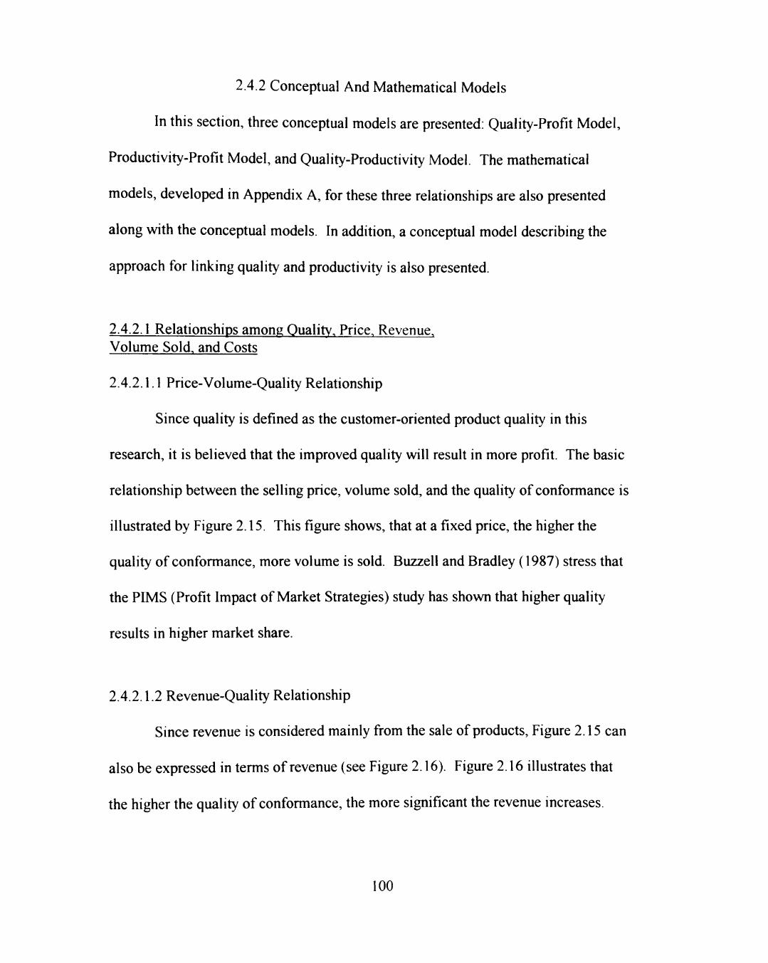
2.4.2 Conceptual And Mathematical Models
In this section, three conceptual models are presented: Quality-Profit Model,
Productivity-Profit Model, and Quality-Productivity Model. The mathematical
models, developed in Appendix A, for these three relationships are also presented
along with the conceptual models. In addition, a conceptual model describing the
approach for linking quality and productivity is also presented.
2.4.2.1 Relationships among Quality, Price. Revenue. Volume Sold, and Costs
2.4.2.1.1 Price-Volume-Quality Relationship
Since quality is defined as the customer-oriented product quality in this
research, it is believed that the improved quality will result in more profit. The basic
relationship between the selling price, volume sold, and the quality of conformance is
illustrated by Figure 2.15. This figure shows, that at a fixed price, the higher the
quality of conformance, more volume is sold. Buzzell and Bradley (1987) stress that
the PIMS (Profit Impact of Market Strategies) study has shown that higher quality
results in higher market share.
2.4.2.1.2 Revenue-Quality Relationship
Since revenue is considered mainly from the sale of products. Figure 2.15 can
also be expressed in terms of revenue (see Figure 2.16). Figure 2.16 illustrates that
the higher the quality of conformance, the more significant the revenue increases.
100
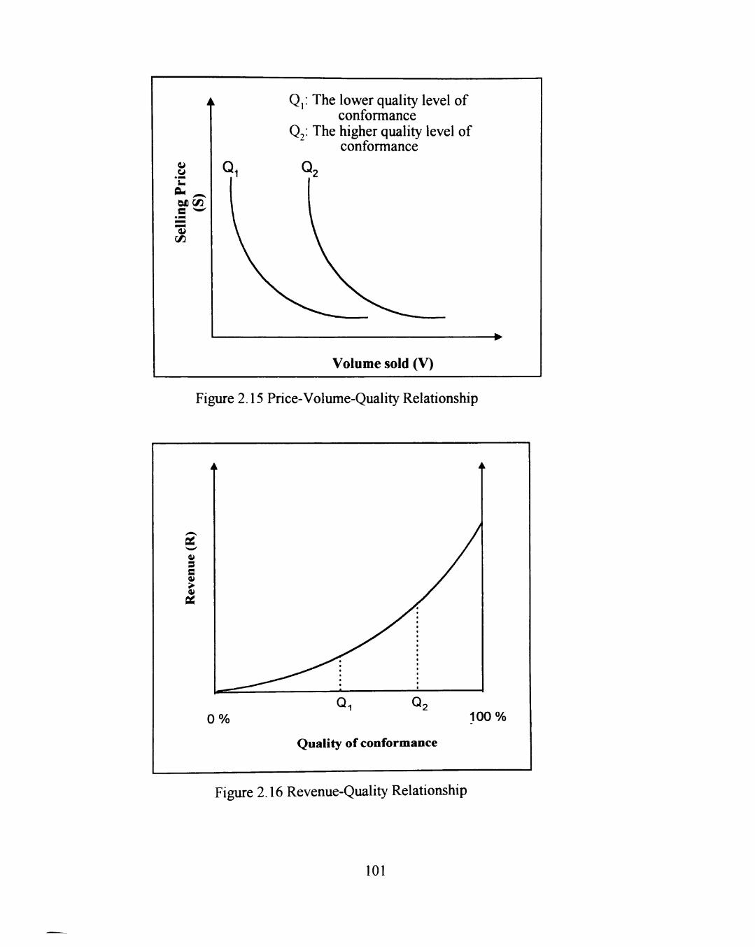
.S ^^
Q,: The lower quality level of conformance
Qj: The higher quality level of conformance
Volume sold (V)
Figure 2.15 Price-Volume-Quality Relationship
i
o s s V > « X
L
0 % Qi Q2
Quality of conformance
i k
100%
Figure 2.16 Revenue-Quality Relationship
101
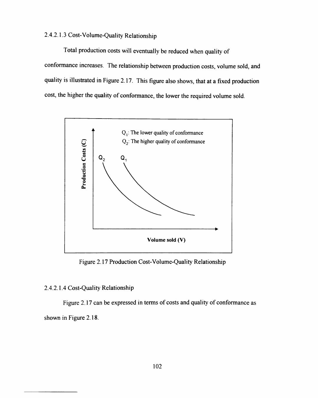
2.4.2.1.3 Cost-Volume-Quality Relationship
Total production costs will eventually be reduced when quality of
conformance increases. The relationship between production costs, volume sold, and
quality is illustrated in Figure 2.17. This figure also shows, that at a fixed production
cost, the higher the quality of conformance, the lower the required volume sold.
i
(J)
Cos
ts
Prod
ucti
on
k
Q2
Q,: The lower quality of conformance
Q^: The higher quality of conformance
Q,
Volume sold (V)
Figure 2.17 Production Cost-Volume-Quality Relationship
2.4.2.1.4 Cost-Quality Relationship
Figure 2.17 can be expressed in terms of costs and quality of conformance as
shown in Figure 2.18.
102
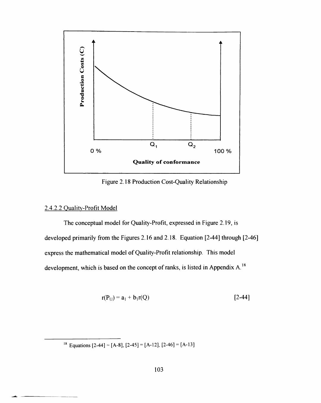
o U e o
'•5
3
0
CL
0% Q i Q.
100%
Quality of conformance
Figure 2.18 Production Cost-Quality Relationship
2.4.2.2 Quality-Profit Model
The conceptual model for Quality-Profit, expressed in Figure 2.19, is
developed primarily from the Figures 2.16 and 2.18. Equation [2-44] through [2-46]
express the mathematical model of Quality-Profit relationship. This model
development, which is based on the concept of ranks, is listed in Appendix A 18
r(Pu) = ai + bir(Q) [2-44]
•' Equations [2-44] = [A-8], [2-45] = [A-12], [2-46] = [A-13]
103

Zr(Q,)r(P^.)-n(n+l)'/4 bi = ^ V - [2-45]
Z[r(Q.)]'-n(n +1)^/4 i = l
ai = (l-bi)(n+l)/2 [2-46]
where
Pu: Unit Profit
Q: Quality conformance level (%)
r(Pu,): the ith rank of Pu in an ascending Pu series
r(Q,): the ith rank of Q in an ascending Q series
n: number of paired data.
Figure 2.19 depicts that the break-even point ofthe quality of conformance is
located at the point where the unit revenue is equal to the unit total input.
104
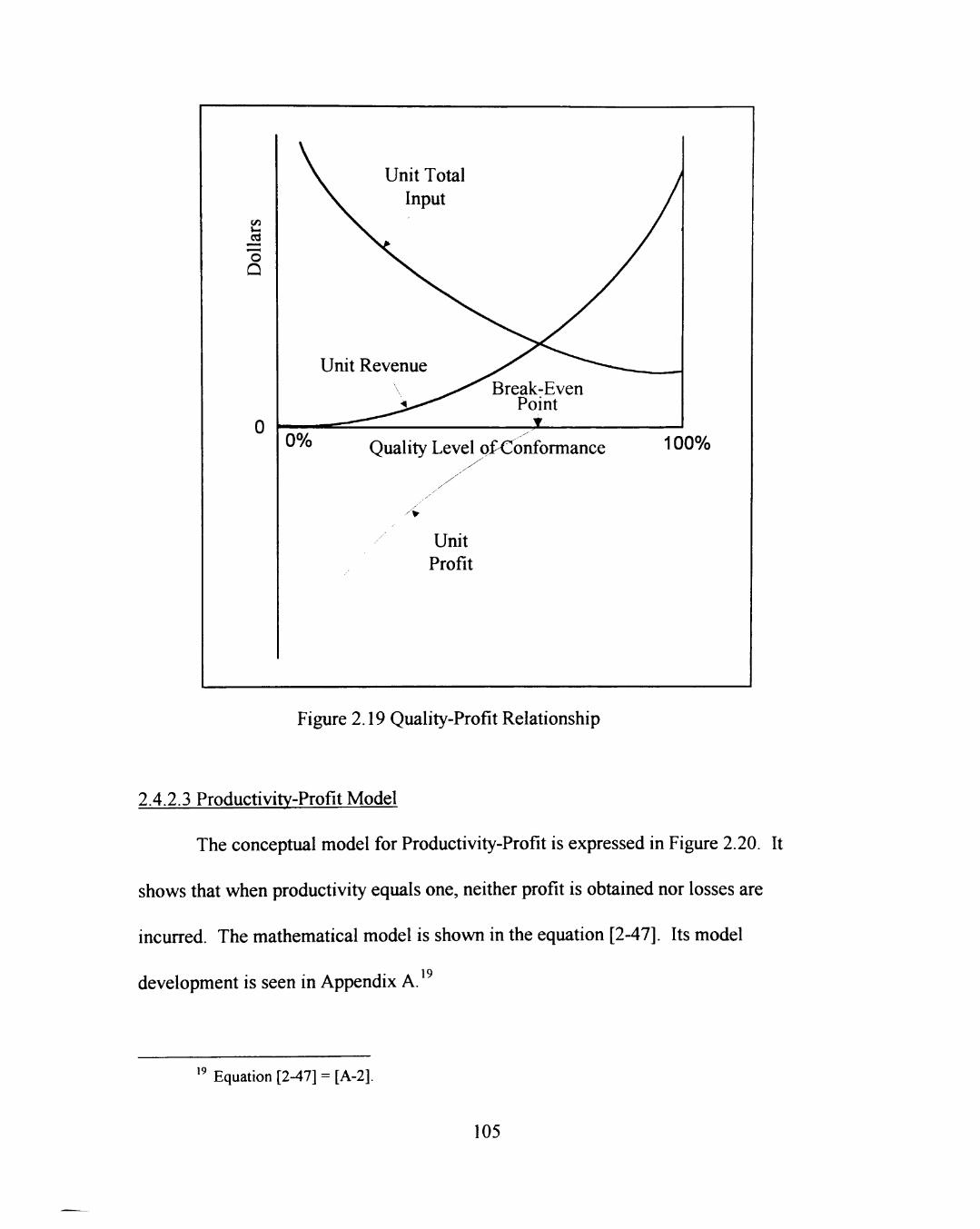
Vi
B 'o O
0 Quality Level ofConformance 100%
Unit Profit
Figure 2.19 Quality-Profit Relationship
2.4.2.3 Productivity-Profit Model
The conceptual model for Productivity-Profit is expressed in Figure 2.20. It
shows that when productivity equals one, neither profit is obtained nor losses are
incurred. The mathematical model is shown in the equation [2-47]. Its model
development is seen in Appendix A. 19
19 Equation [2-47] = [A-2].
105
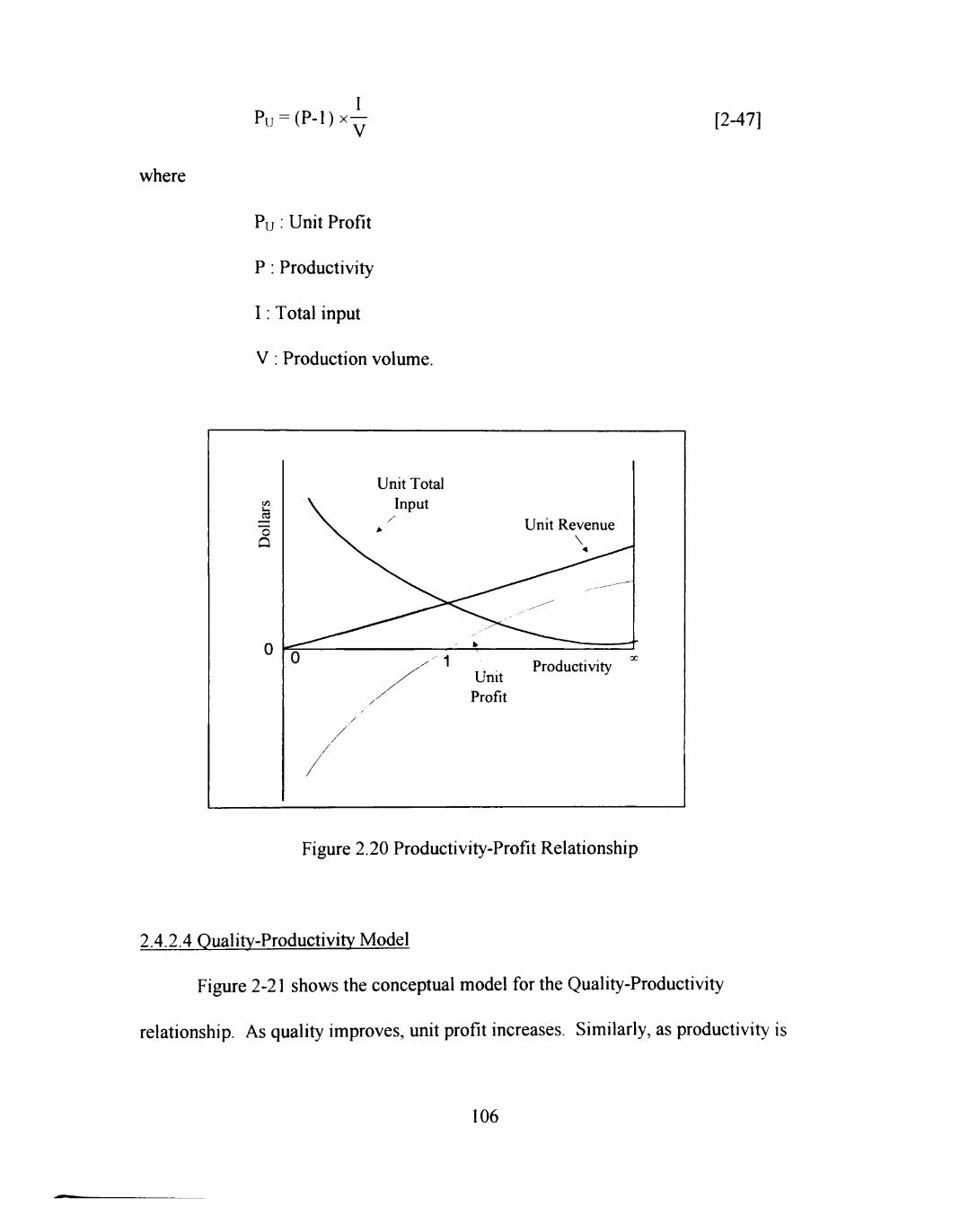
Pu = (P-l)x:|^ [2-47]
where
Pu: Unit Profit
P : Productivity
I : Total input
V: Production volume.
o D
olla
rs
0
/
/
Unit Total Input
/ 1
/
*^
Unit Profit
Unit Revenue \
oc
Productivity
Figure 2.20 Productivity-Profit Relationship
2.4.2.4 Quality-Productivity Model
Figure 2-21 shows the conceptual model for the Quality-Productivity
relationship. As quality improves, unit profit increases. Similarly, as productivity is
106

enhanced, unit profit also increases. Hence, quality and productivity go hand-in-
hand. Equations [2-48] through [2-50] exhibit the mathematical model for Quality-
Productivity relationship. This model development is also listed in Appendix A
This model is also developed based on ranks.
20
C30
O
O
&a
P=l
Q=o
-oo
P X ^ BEP /
Pr A
of rej
it; ; I M :
100
jr \ Quality Loss >^ o /f»/ X ^ BEP (% Area yr
)
Figure 2.21 Quality-Productivity Relationship
20 Equations [2-48] = [A-23], [2-49] = [A-24], [2-50] = [A-25].
107
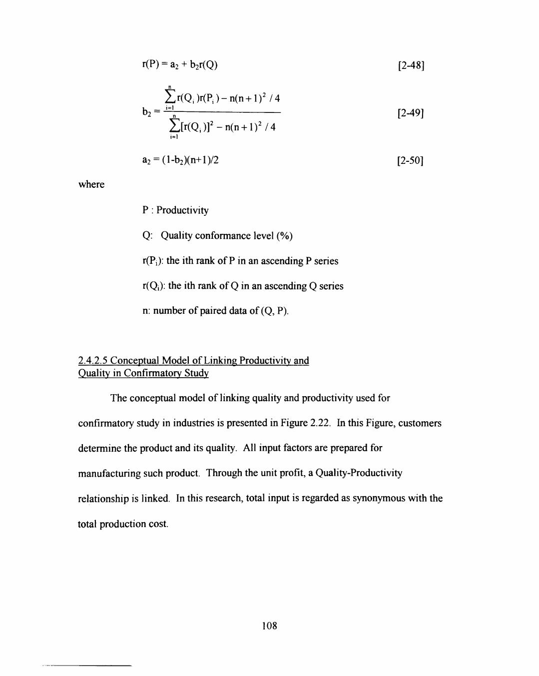
r(P) = a2 + b2r(Q) [2-48]
n
Zr(Q.)r(P.)-n(n + l )^ /4 b2 = —^ [2-49]
Z[ r (Q. ) ] ' -n (n +1)^/4 i= l
a2 = (l-b2)(n+l)/2 [2-50]
where
P : Productivity
Q: Quality conformance level (%)
r(Pi): the ith rank of P in an ascending P series
r(Q,): the ith rank of Q in an ascending Q series
n: number of paired data of (Q, P).
2.4.2.5 Conceptual Model of Linking Productivity and Quality in Confirmatory Study
The conceptual model of linking quality and productivity used for
confirmatory study in industries is presented in Figure 2.22. In this Figure, customers
determine the product and its quality. All input factors are prepared for
manufacturing such product. Through the unit profit, a Quality-Productivity
relationship is linked. In this research, total input is regarded as synonymous with the
total production cost.
108
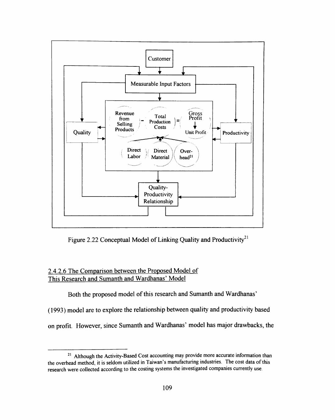
^ r
Quality — •
V
Customer
T V
Measurable Input Factors
n
Revenue ^ ^ t Gross from ,_ „ Total p^fi t ^
Selling / P ^ ^ - ^ - )-l 1 , Products Costs ^J^^^^^^,
I Direct \i Direct W Over- \ Labor ,' Material A head^' j
h
i Quality-
Productivity Relationship
—^
^ r 1
Productivity
^ '
Figure 2.22 Conceptual Model of Linking Quality and Productivity '
2.4.2.6 The Comparison between the Proposed Model of This Research and Sumanth and Wardhanas' Model
Both the proposed model of this research and Sumanth and Wardhanas'
(1993) model are to explore the relationship between quality and productivity based
on profit. However, since Sumanth and Wardhanas' model has major drawbacks, the
' Although the Activity-Based Cost accounting may provide more accurate information than the overhead method, it is seldom utilized in Taiwan's manufacturing industries. The cost data of this research were collected according to the costing systems the investigated companies currently use.
109
proposed model of this research is more appropriate to explain the profit-based
Quality-Productivity relationship. The three major drawbacks of Sumanth and
Wardhanas' model are described in the following.
1. The term "cost" used in Sumanth and Wardhanas' model is not congruent.
Sumanth and Wardhanas' model was developed by combining two models,
Dawes' model of quality of conformance and Sumanth's Total Productivity Model
(TPM). The cost used in Dawes' model was the "quality cost," while in Sumanth's
TPM was the "input cost." The term "quality cost" is not equivalent to "input cost,"
neither in concept nor in mathematics. Hence, the quality-productivity model
resulting fi-om combining these two models based on different cost bases is
questionable.
2. The relationship between profit and costs in Sumanth and Wardhanas'
model is not clear.
This drawback relates to the first drawback. Since profit is gained by
subtracting the costs, and costs are explained in two different ways in Sumanth and
Wardhanas' model, the calculation of profit is also questionable. Qriginally, in
Sumanth's TPM, profit is linearly related to input cost. However, in their final
model, profit is calculated by comparing with quality costs. This would result in a
question as to the meaning of what profit stands for in their model.
3. The cost category in Sumanth and Wardhanas' model may not be
applicable to all industries.
110
In Sumanth and Wardhanas' model, the input costs are primarily classified
into human, material, capital, energy, and other expense. This classification is
originally designed for calculating partial productivity. However, this classification
may not be adopted by industries in calculating the product costs.
The proposed mathematical models of this research overcomes the major
drawbacks in Sumanth and Wardhanas' model. Compared with the Sumanth and
Wardhanas' model, these proposed models have the following major merits:
1. Production cost is more practically used than quality cost.
Quality cost is an excellent concept in quality management; however, it is
seldom employed in the cost accoimting system in the real world. This is
because quality cost does not equal production cost. Under the most
current accounting system, production cost is a better measure because it
directly affects profit. So far, there is no accurate and detailed criteria to
calculate quality costs for general purpose. From the practical view points,
production cost is more likely to be calculated and applied.
2. Profit and revenue are clearly defined in the proposed models
In addition to the income from selling products, there are many other
sources of revenue. For instance, investment income or gains on disposal
of fixed assets are not imusual in a company. These non-operating revenue
also affect profit; however, they apparently have nothing to do with the
productivity or product quality. The proposed models of this research
111
concentrates on the revenue from selling products. In addition, profit is
defined as the before-tax gross profit and is simply obtained by subtracting
total cost from total revenue.
3. Instead of directly measuring the Quality-Productivity relationship by using
ratio scale or interval scale of measurements, it is more appropriate to
measure it with ordinal scale of measurement.^^
Quality, as well as productivity, can be defined in hundreds of ways. For
example, number of defects per 100 pieces or one lot, or per 1000 yards,
etc. Only when these data are converted to conformance level % can they
be used to relate to other variables. These transformed data are not the
data of ratio scale. It is questionable that Sumanth and Wardhanas' model
uses these potential ordinal data to establish their formula. The proposed
models, especially Quality-Profit and Quality-Productivity models, utilize
the concept of ranks to compare the relationships between variables. This
approach does not necessarily need interval or ratio data, ordinal data is
enough for the analysis.
^ According to Conover (1980), an ordinal scale of measurement "refers to measurements where only the comparisons 'greater,' 'less,' or 'equal' between measurements are relevant." The interval scale of measurement considers "not only the relative order ofthe measurements as in the ordinal scale but also the size ofthe interval between two measurements." In addition to the order and interval size, a ratio scale of measurement must also have a meaningful ratio between two measurements. The distinction between the ratio scale and the interval scale is that the ratio scale has a natural zero measurement, while the zero measurement of interval scale is defined arbitrarily.
112
2.4.2.7 Advantages of Relating Quality-Profit and Quality-Productivity Models Based on Ranks
Because ofthe deficiencies and limitations of current mathematical models
addressed in sections 2.3 and 2.4.2.6, this research proposed the Quality-Profit and
Quality-Productivity models based on ranks. The reasons, also the advantages, for
using the concept of ranks for developing models of this research are:
1. Models based on ranks are more generalizable.
Different manufacturing environments have their own features, except
for the use ranks, it is hard to find a unique model to relate quality, profit,
and productivity for all cases.
2. Models based on ranks are more reliable.
Data used in the models based on ranks do not need accurate as the original
data. Therefore, ranks may reduce the effects caused by original data bias
or errors.
3. Models based on ranks can be applied to various definitions of quality,
productivity, and profit.
By using ranks, the problem of different definitions for variables can be
eliminated in a model based on ranks.
4. Models based on ranks can avoid the problem of misusing measurement
scales.
When quality can only be measured using an ordinal measurement scale, it
is unreasonable to relate the quality data to a model based on interval or
113
ratio scales of measurement. However, by using ranking, this type of
quality data can be utilized in a model based on ranks.
2.4.2.8 Contributions of This Research
The contributions of this research are addressed from both theoretical and
practical standpoints. The theoretical contributions of this research lie mainly in the
development of proposed mathematical model. Specifically, there are three points
viewed as contributions in theory.
1. The proposed model is the first model to use nonparametric statistical
approach to establish the mathematical models for Quality-Profit and
Quality-Productivity relationships.
2. The positive relationships of Quality-Profit, Productivity-Profit, and
Quality-Productivity are proved through the proposed mathematical
models.
3. The proposed model is the first one to utilize the concept of unit profit to
compare with Quality, Productivity, and be a base for relating Quality-
Productivity and to establish models for them. Unit profit is more
meaningful because total profit is tremendously affected by sales quantity.
The practical contributions of this research are:
1. The proposed model is the first model used for a confirmatory study on the
Quality-Productivity relationship in manufacturing companies.
114

2. Through the field study, the positive relationship between quality and
productivity are confirmed and validated by this research.
115
CHAPTER 3
RESEARCH METHODOLQGY
Research methodology is a way of solving problems (Leedy, 1993).
Therefore, the research process is first addressed to describe the way this study
proceeds. Following this research process, methodological issues regarding research
design, data collection and treatment, measurements, and constraints are presented.
3.1 Research Process
Research process describes the steps a study follows. Figure 3.1 illustrates the
research process of this study which are discussed in the following.
1. Research statement
The research statement, delineated in Chapter 1, illustrates the outline
of this research, including the following: problem statement, scope of
research, limitations and assumptions, research needs and benefits, and
expected results.
2. Literature review and models
This step was covered in Chapter 2 which stems from the literature
review and follows the conceptual models and mathematical models.
3. Research design
The research design is discussed in section 3.2.
116
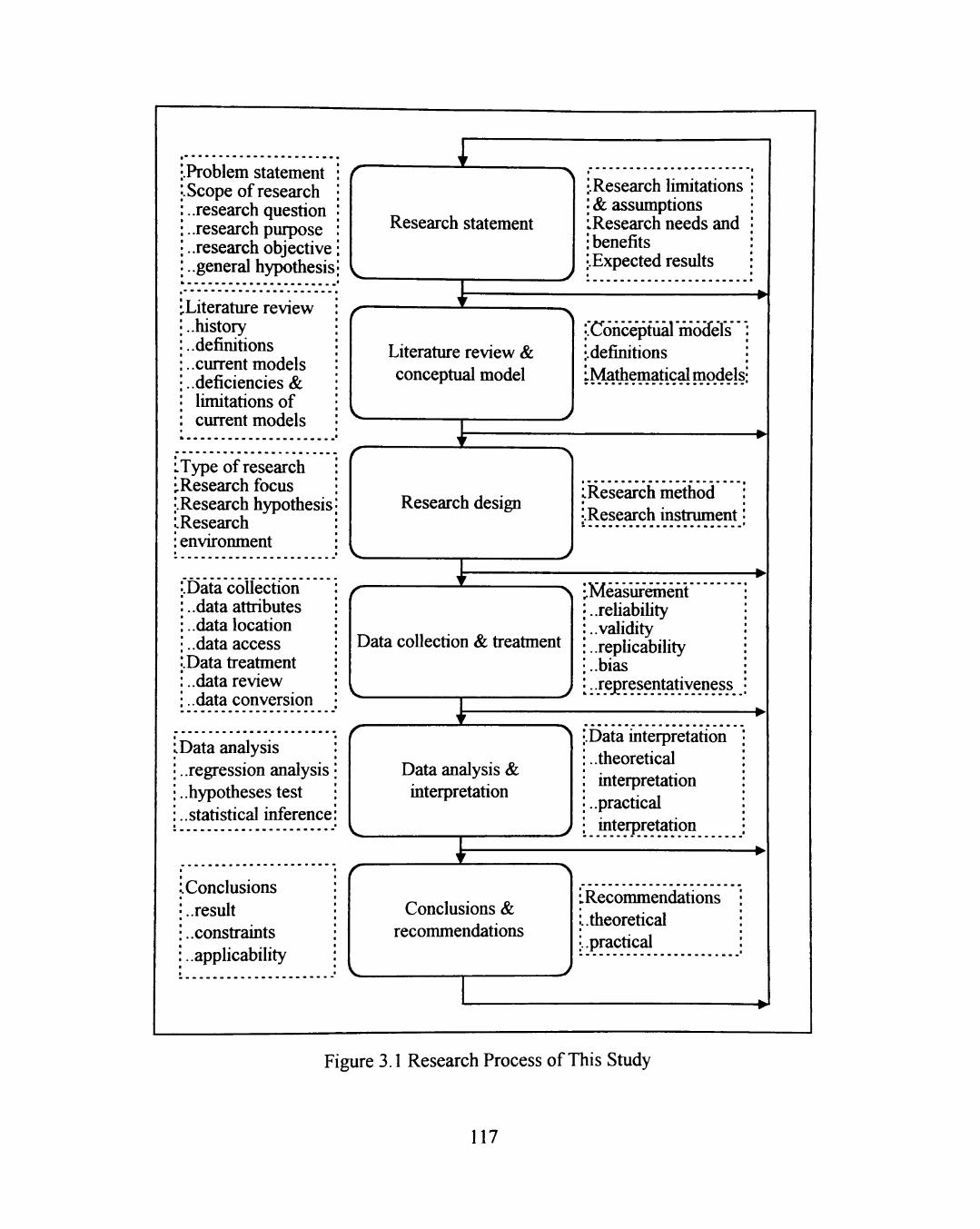
•.Problem statement |. Scope of research :..research question : ..research purpose j ..research objective : ..general hypothesis
•.Literature review • ..history :.. definitions '..current models •..deficiencies & : limitations of •
: current models
.Type of research •.Research focus ;. Research hypothesis I Research ; environment
j.Data collection :..data attributes •..data location •..data access j.Data treatment :.. data re view '..data conversion
iData analysis .regression analysis .hypotheses test .statistical inference:
:. Conclusions ^.resuh •
•..constraints i.apphcability
Research statement
Research limitations & assimiptions Research needs and benefits Expected results
Literature review & conceptual model
^Conceptual "mocfels' •.definitions LMathematical models:
^ r
Research design
>
iResearch method : • I
vResearch instrument '• 1 t
Data collection & treatment
•.Measiirement • ..rehabiUty :.. validity i.repUcability •..bias
Data analysis & interpretation
•.Data interpretation : ..theoretical : interpretation :..practical : interpretation
Conclusions & recommendations
iRecommendations :..theoretical •
[..practical
Figure 3.1 Research Process of This Study
117
4. Data collection and treatment
The methodology of data collection and treatment are addressed in
the section 3.3 of this chapter. Issues regarding data measurement,
reliability, validity, replicability, bias, and representativeness are discussed
in Section 3.4. In addition, some research constraints are presented in the
last section of this chapter.
5. Data analysis and interpretation
This step is conducted after data is collected. The statistical
approach is the primary tool in data analysis. Results of data analysis
are interpreted theoretically and practically.
6. Conclusions and recommendations
The last step of this research is to summarize the results and draw
conclusions. Suggestions for fiulher research may be made based on the
results of this study.
The research process constructs the framework of this research. The following
chapters and sections proceed according to this framework.
3.2 Research Design
The purpose of research design is to provide a plan for research. In this
section, the following issues are addressed: type of research, research focus, research
hypotheses, research environment, research method, and research instrument.
118
3.2.1 Type of Research
This research is basically classified as quantitative. Because it investigates
the relationship between quality and productivity based on profit, much numerical
data are required to develop and verify the relationship.
This research can also be classified as an empirical confirmatory study. Two
cases studies were conducted in Taiwan's industries to confirm the positive
relationship between quality and productivity. In addition, because a practical
solution is sought for manufacturing systems, this research may also be considered
applied research.
Because this research is to conduct a confirmatory study, its research logic is
essentially deductive. However, during the research process, the mathematical
models developed for each relationship among quality, productivity, and profit
require inductive logic to lead to a specific model. Therefore, although the overall
research is deductive, the logic of model development is inductive. Thus, it can be
stated that this research is a quantitative-deductive-applied-confirmatory research
project.
3.2.2 Research Focus
This research focuses mainly on three issues as follows:
I. Study the relationship between product quality and unit profit for
manufacturing products.
119
2. Study the relationship between productivity and unit profit for
manufacturing products.
3. Study the quality-productivity relationship based on unit profit for
manufacturing products.
The definitions of quality and productivity used in this research are presented
in sections 2.4.1.1 and 2.4.1.2. Profit used for comparing and relating with variables
is unit profit, which is an average profit per product.
In addition to the above issues, the following secondary issues closely related
to the main issues are also investigated:
1. Whether the proposed Quality-Profit relationship model is applicable in a
manufacturing system.
2. Whether the proposed Productivity-Profit relationship model is applicable
in a manufacturing system.
3. Whether the proposed Quality-Productivity relationship model is applicable
in a manufacturing system.
3.2.3 Research Hypotheses
This research has a main hypotheses and two sub-hypotheses. Figure 3.2
states the main hypotheses and Figure 3.3 states the sub-hypotheses. Both main
hypotheses and sub-hypotheses are tested. The purpose of these hypotheses tests is to
verify the relationships identified in the mathematical models.
120

Main Hypotheses
In a manufacturing company, the productivity levels of a product have a
probability distribution that is positively dependent ofthe levels of product
quality of conformance of that product.
That is, if Qi denotes the conformance level at time i of a product and P,
represents the productivity level resulting from Qi at time i, and if
Qj >Qj , foranyi, j =1 , 2, ..., n, i^j,
then, the null and alternative hypotheses are
H„: P; ^ P,
H,:P, >P,
respectively.
Figure 3.2 Main Hypotheses of This Research
121
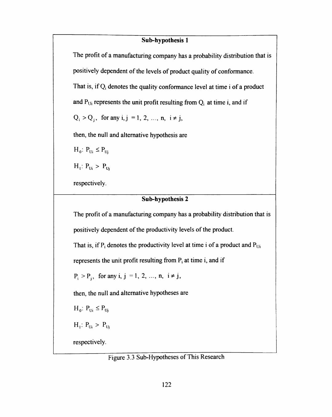
Sub-hypothesis 1
The profit of a manufacturing company has a probability distribution that is
positively dependent ofthe levels of product quality of conformance.
That is, if Q, denotes the quality conformance level at time i of a product
and Pu, represents the unit profit resulting from Q, at time i, and if
Qi >Qj , foranyi,j =1 , 2, ..., n, i;«tj,
then, the null and alternative hypothesis are
H„: Pu; ^ Pu,
H,: Pu, > Pu,
respectively.
Sub-hypothesis 2
The profit of a manufacturing company has a probability distribution that is
positively dependent ofthe productivity levels ofthe product.
That is, if P, denotes the productivity level at time i of a product and Pu,
represents the unit profit resulting from P, at time i, and if
Pi >Pj, foranyi, j =1 , 2, ..., n, i^],
then, the null and alternative hypotheses are
HQ- Pui - Puj
Hp Pu, > Puj
respectively.
Figure 3.3 Sub-Hypotheses of This Research
122
3.2.4 Research Environment
This confirmatory study were conducted at two companies in Taiwan.
Because the companies requested to remain anonymous, their names were replaced
by ABC Company and XYZ Company, respectively, throughout this research. Both
companies were invested in by Taiwan entrepreneurs. The ABC Company was
typically a traditional industrial company. The XYZ Company represented a newly
developing industry in Taiwan. The following two subsections present a brief
overview for each company.
3.2.4.1 ABC Company
ABC Company, at the time ofthe study, was one ofthe leading companies in
Taiwan's textile industry. The capitalization of ABC Company in 1995 was 120
million equivalent US dollars. The textile revenue in 1995 was an estimated 113
million US dollars, accounting for about 83 % ofthe company's total operating
revenue. This company had eight factories scattered in northern and central Taiwan.
Each factory was engaged in different processes of products. Due to time and cost
constraints, three factories which were located closely in northern Taiwan were
selected for study.
The factory produced five products: gingham, piece-dyed fabric, chambray,
denim, and printed flannel. The main customers of these products were from the
USA, Southeast Asia, and Hong Kong. Among the products, gingham and piece-dyed
123
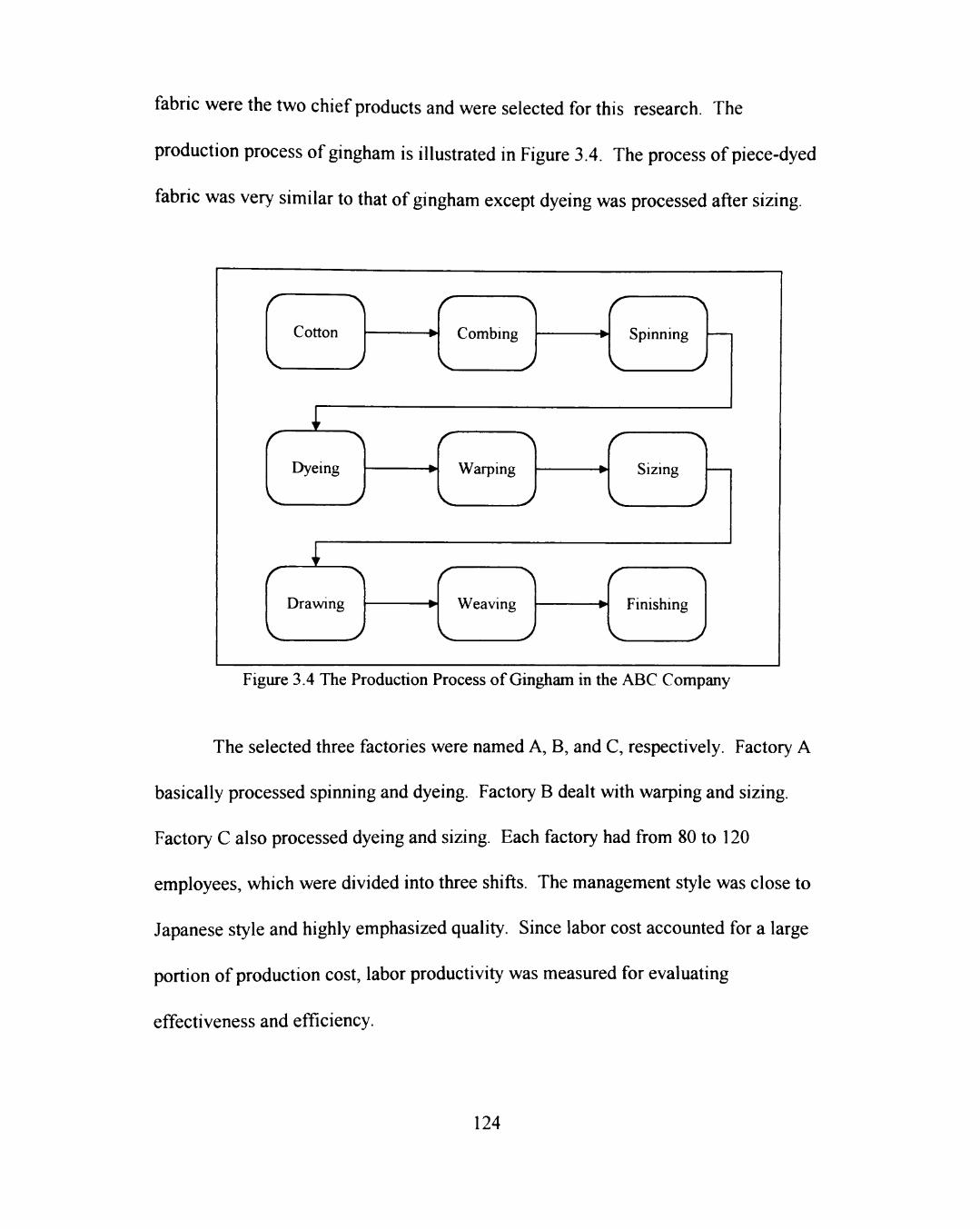
fabric were the two chief products and were selected for this research. The
production process of gingham is illustrated in Figure 3.4. The process of piece-dyed
fabric was very similar to that of gingham except dyeing was processed after sizing.
Cotton
^'
Dyemg
r r ^
Drawing
r ^ Combmg
Warpmg
Weaving
W
Spinning
Sizing
Finishing
I J Figure 3.4 The Production Process of Gingham in the ABC Company
The selected three factories were named A, B, and C, respectively. Factory A
basically processed spinning and dyeing. Factory B dealt with warping and sizing.
Factory C also processed dyeing and sizing. Each factory had from 80 to 120
employees, which were divided into three shifts. The management style was close to
Japanese style and highly emphasized quality. Since labor cost accounted for a large
portion of production cost, labor productivity was measured for evaluating
effectiveness and efficiency.
124
3.2.4.2 XYZ Company
XYZ Company, at the time ofthe study, was a manufacturer of network
products in Taiwan. It was established in 1989 in northern Taiwan. The
capitalization of XYZ Company in 1996 was US$ 13.1 million. This company had
nearly 80 employees and the sales revenue was US$ 7.8 million in 1995.
The major products of XYZ Company were Token Ring, Ethernet, Remote
Access, SOHO (Small Office, Home Office) Network, Wireless LAN (Local Area
Network). Most ofthe customers were scattered around the world, especially the
developed countries. In America, the US Air Force, JC Penny's, Chemical Bank,
GTE, and Chevron were their major customers.
In its business activities, the XYZ Company had engaged in partnerships with
industry leaders and customers. Among XYZ's partnerships were its relationships
with Token Ring industry leader, IBM, and Ethernet industry leader, Novell. These
industry partnerships had led the XYZ Company to develop easier to use and install
products.
The XYZ Company emphasized R&D as well as production. However,
design was usually the most critical problem in this company. In order to meet fast
development in PC network applications, the XYZ Company employed nearly one
third of its employees in R&D. More than half of these R&D engineers possess
master degrees in Electronic or Control Engineering. The production department
also had more than one third ofthe employees. Product quality must be 100%
125
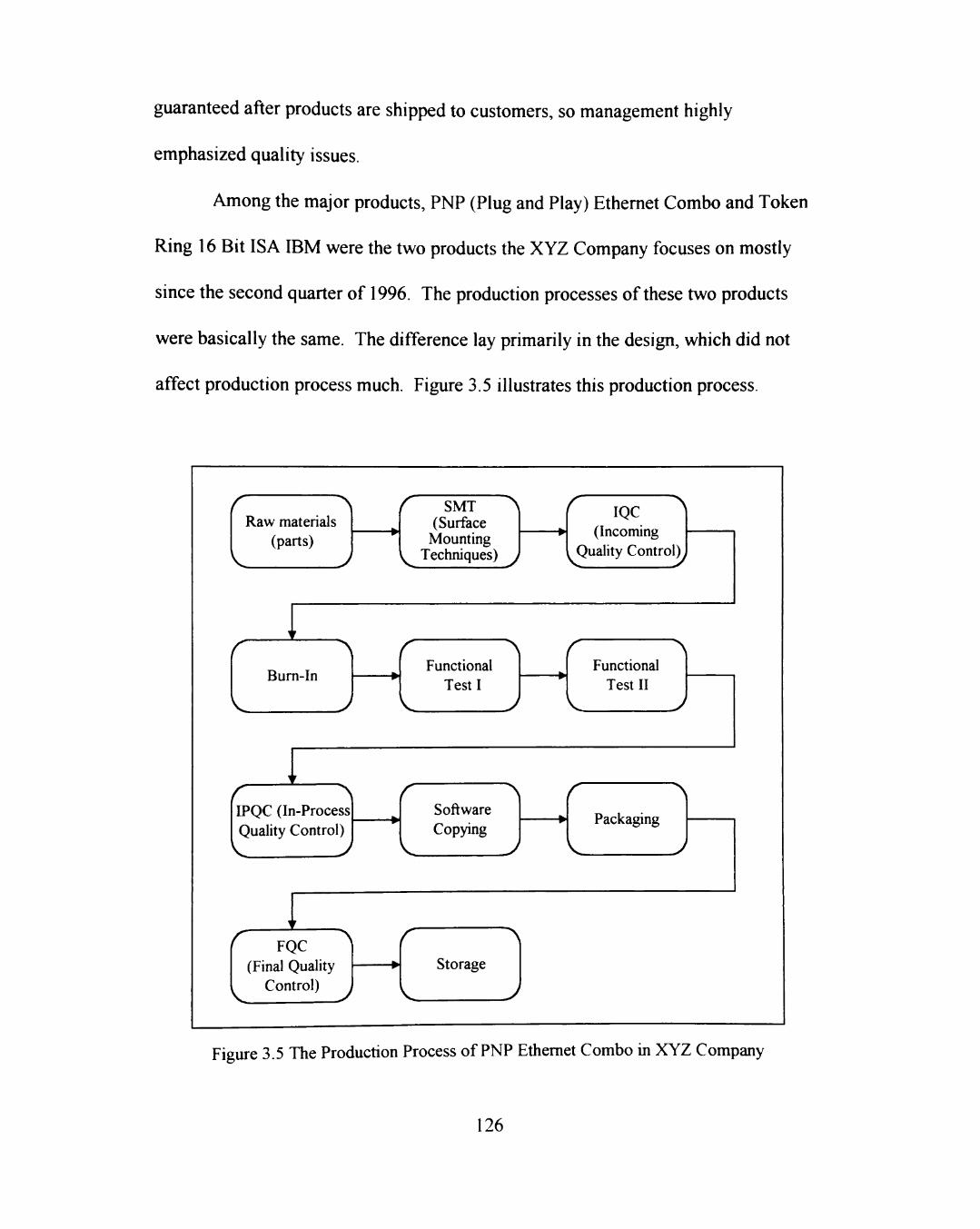
guaranteed after products are shipped to customers, so management highly
emphasized quality issues.
Among the major products, PNP (Plug and Play) Ethernet Combo and Token
Ring 16 Bit ISA IBM were the two products the XYZ Company focuses on mostly
since the second quarter of 1996. The production processes of these two products
were basically the same. The difference lay primarily in the design, which did not
affect production process much. Figure 3.5 illustrates this production process.
( \ Raw materials
(parts)
•y r
Bum-In
^ r r ^ IPQC (In-Process Quality Control)
\ r
^ FQC ^ (Final Quality
Control)
r SMT ^ (Surface Mounting
k Techniques) j
^ IQC ^ (Incoming
, Quality Control),
r > Functional
Test I
( \ Software Copying
^ J
Storage
r ^ Functional
Test II
Packaging
Figure 3.5 The Production Process of PNP Ethernet Combo in XYZ Company
126
3.2.5 Research Method
The method used by this research in the selected companies is depicted by
Figure 3.6. The task force in each company assisted the research by participating
discussion for definitions, terms, supporting required data, reviewing collected data,
and providing other services, such as process and product introduction, and
professional opinions. Statistical analysis, including hypotheses testing and
regression analysis, was done by the researcher. Model verification and
interpretation for the results were completed after the statistical analysis.
3.2.6 Research Instrument
The instruments used in this research are as follows:
1. Statistical tool: Regression analysis in Excel 5.0, nonparametric statistical
program from Dr. W J. Conover.
2. Personal computer (CPU 486DX2-66) and associated software (VISIO 4.0,
WORD 6.0).
3.2.7 Measurement of Costs and Profit
Profit is a key variable in this research. It is used for linking with Quality and
Productivity respectively. As defined in section 2.4.1.3, profit is obtained by
subtracting production cost from revenue in this research. Hence, it is necessary to
describe the measurement of costs and profit. The measurement of production costs
127
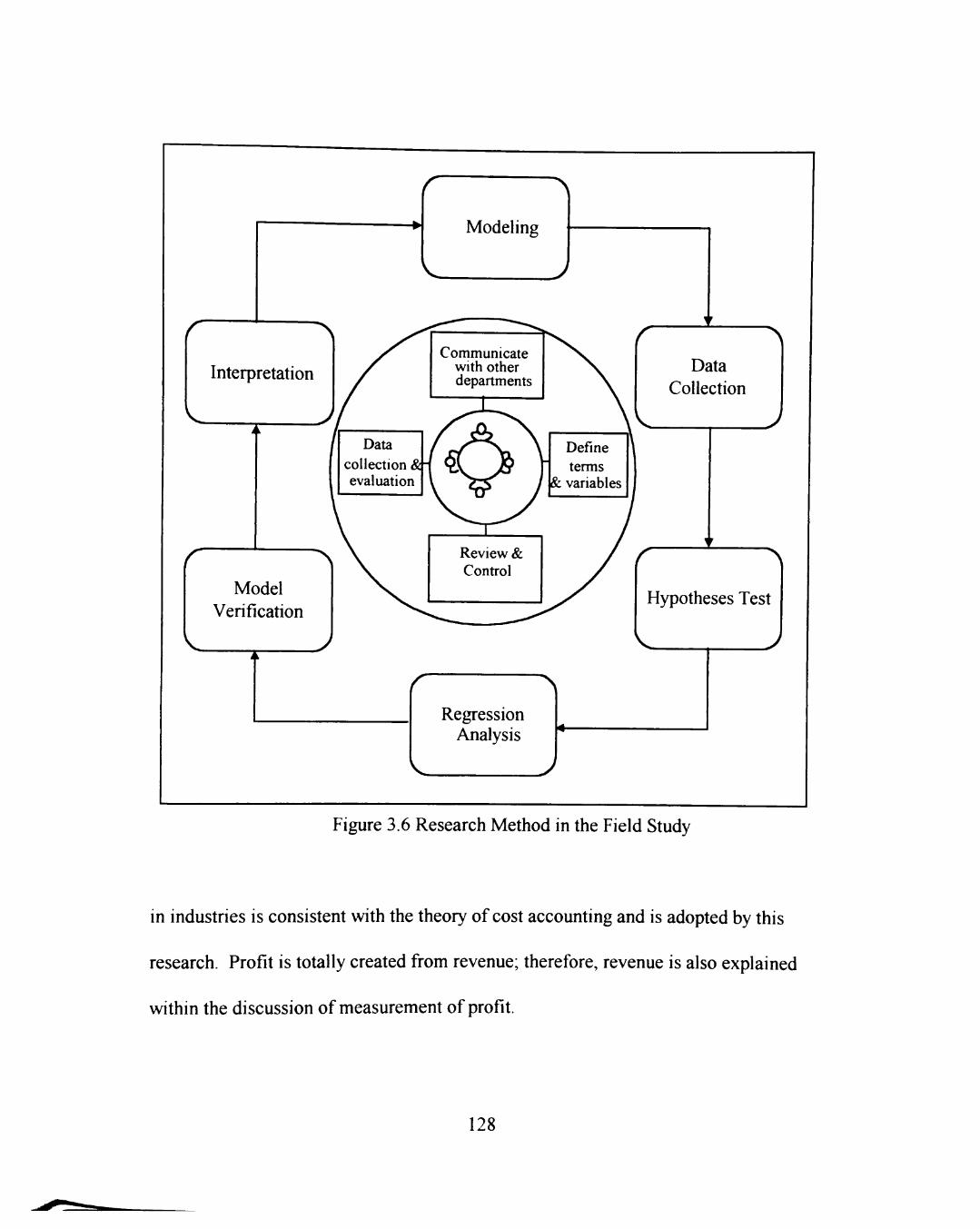
r
• ^
Modeling
Interpretation
r Model
Verification
Data Collection
Hypotheses Test
Regression Analysis
Figure 3.6 Research Method in the Field Study
in industries is consistent with the theory of cost accounting and is adopted by this
research. Profit is totally created from revenue; therefore, revenue is also explained
within the discussion of measurement of profit.
128
3.2.7.1 Measurement of Costs
As addressed in section 2.4.1.4, cost is referred to production cost and is
classified into direct material, direct labor, and overhead in this research. The
problem in measuring production cost lies primarily in the allocation of overhead.
The base of overhead allocation must be first considered. Although there are several
bases, such as direct labor hour or direct labor cost, etc., it must be recognized that no
unique base is perfect for all industries.
The bases of allocating overhead in this research were depended upon the
allocation system currently used by the companies. In other cases, the bases may be
determined according to the following:
1. Cost unit base— if the unit cost of each product is known.
2. Volume base— if products and their manufacturing processes are similar.
3. Direct material base-- if direct material cost is higher than direct labor cost.
4. Direct labor base- if direct labor cost is higher than direct material cost.
5. Machine hour base-- if machine hours of manufacturing products are
Known.
3.2.7.2 Measurement of Profit
As defined in section 2.4.1.3, profit is the difference between revenue and
production cost. If the cost is known, then profit is determined by revenue, which is
the product of selling price times sales quantity. Selling price is determined by the
129
company and market/customer. Sales quantity is measured per order or lot.
Therefore, profit is measured by an order or a lot. However, because it is most likely
that the product quantity in each lot or order varies, it is necessary to use the unit
profit (profit per piece) as the base in comparing with quality or productivity.
In order to avoid misconstruing the quality-productivity relationship by other
unrelated factors, the revenue in this research is totally from the sale of products.
Other income not directly from the sale of products, such as the disposal on fixed
assets or the investment income, are not considered revenue in this research.
3.2.8 Test plans of This Research
According to the hypotheses of this research presented in subsection 3.2.3,
three test plans must be established. Figures 3.7, 3.8, and 3.59 illustrate the test plans
for Quality-Profit, Productivity-Profit, and Quality-Productivity relationships
respectively.
3.2.9 Specific Models Establishment
In addition to confirm the relationships among quality, productivity, and
profit, the specific models, Eqs. [3-1] through [3-7], for the investigated products and
companies were also established. These models would help the company realize how
these performance measures, quality, productivity and unit profit relate to each other.
130

1. Test hypotheses: If Q,>Q^, foranyi,j =1, 2, . . . ,n, i 9 j , then
H,:Pu. > Pu,
2. Test data & description:
Product: Location:
Order (Lot) # Prod. Quantity Quality (%) Revenue Production Cost Profit @Profit Other
3. Normality test: (Figure & analysis)
4. Statistical test: (a = 0.05)
5. Conclusion:
Figure 3.7 Test Plan for Quality-Profit Relationship
131
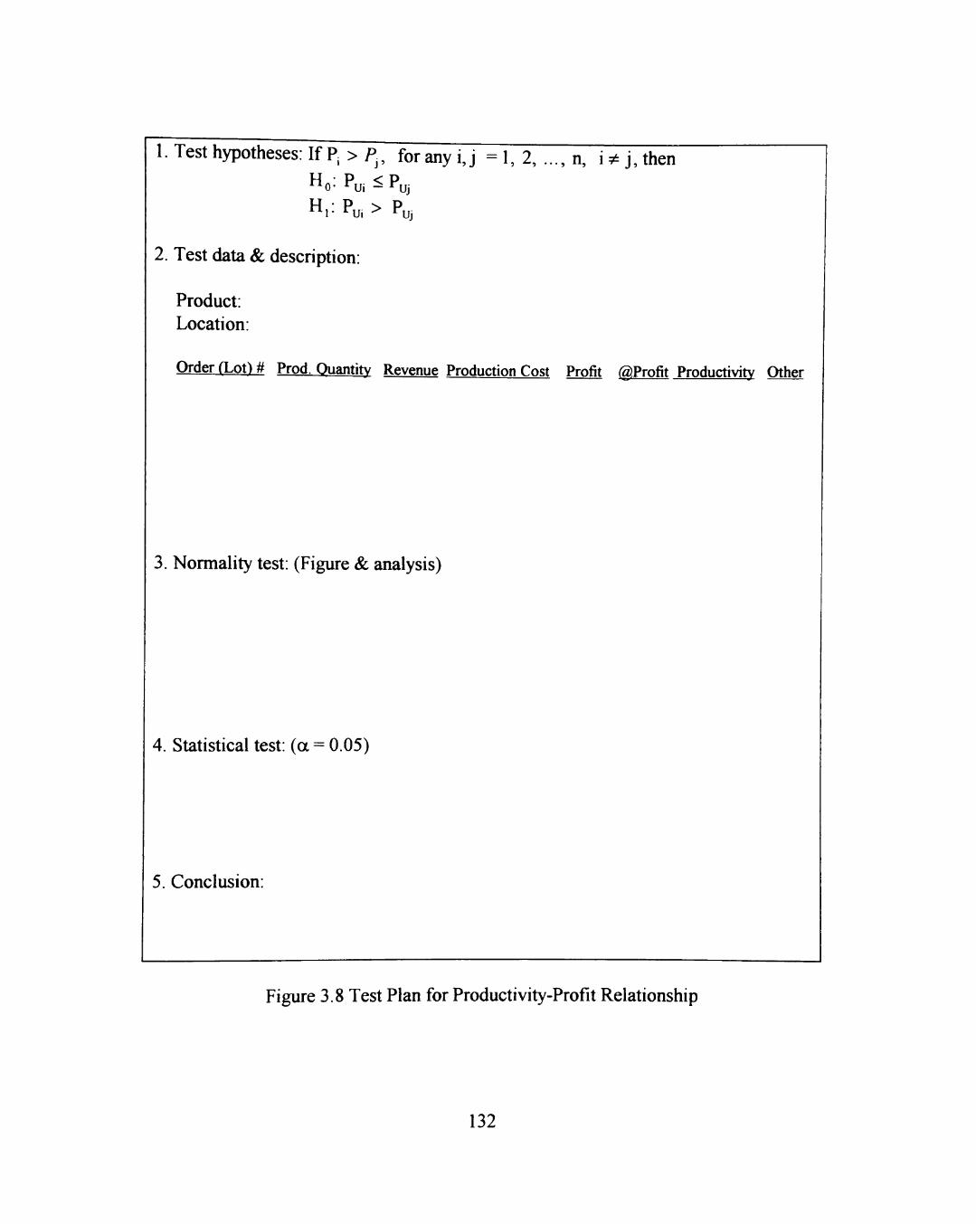
1. Test hypotheses: If p. >P^, foranyi,j =1, 2, . . . ,n, i7ej,then
Ho: Pui ^ Puj
H,: Pu. > Pu,
2. Test data & description:
Product: Location:
Order (Lot) # Prod. Ouantity Revenue Production Cost Profit @Profit Productivity Other
3. Normality test: (Figure & analysis)
4. Statistical test: (a = 0.05)
5. Conclusion:
Figure 3.8 Test Plan for Productivity-Profit Relationship
132
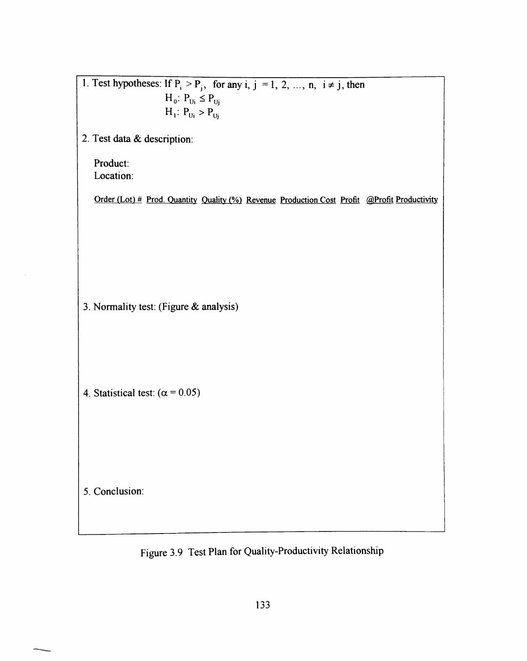
1. Test hypotheses: If P| >Pj, foranyi, j =1, 2, . . . ,n, i?tj,then
Ho: Pu, ^ Puj H,:Pui>Puj
2. Test data & description:
Product: Location:
Order (Lot) # Prod. Ouantity Oualitv (%) Revenue Production Cost Profit (giProfit Productivity
3. Normality test: (Figure & analysis)
4. Statistical test: (a = 0.05)
5. Conclusion:
Figure 3.9 Test Plan for Quality-Productivity Relationship
133
The establishment ofthe specific models are illustrated as follows:
I. Quality-Profit model
Let Q, denote the quality conformance level of ith lot
Pu, denote the unit profit of ith lot
r(Qi): the ith rank in the ascending Q series
r(Pu,): the ith rank in the ascending Pu series.
Then, the model is
r(Pu) = ai + b,r(Q) [3-1]
where
n
Zr(Q,)r(Pu.)-n(n +1)^/4
bi = —r. [3-2] Z[r (Q.) ] ' -n(n +1)^/4 i=l
a, = (l-bi)(n+l)/2. [3-3]
ai and bi are the two constants, which vary with different companies or
products, and n is the number of paired data of (Q, Pu).
2. Productivity-Profit model
Let P, denotes the productivity of ith lot
r(Pi): the ith rank in the ascending P series
I,: the total production cost of ith lot
Y,: The volume produced, including both quality conformed and
nonconformed products, of ith lot.
134
Then,
Pu = ( P - l ) x i - . p.4]
3. Quality-Productivity model
The model is
r(P) = a2 + b2r(Q) [3-5]
where.
n
Zr(Qi)r(P.)-n(n +1)^/4 i=l
b2 = —„ [3-6] £["•(0,)]' - n(n +1)' / 4 i = l
a2 = (l-b2)(n+l)/2. [3-7]
ai and bi are the two constants, which vary with different companies or
products, and n is the number of paired data of (Q, P).
3.2.10 Unit of Analysis
3.2.10.1 ABC Company
The units of analysis in the ABC Company were:
1. 1000 yards Gingham,
2. 1000 yards Piece-dyed fabric.
Cloth is shipped in rolls. However, because ofthe variety of customer
requirements, each roll may have different lengths. Therefore, 1000 yards was set as
the unit for measurement.
135
The unit of measurements in the ABC Company for production cost,
production quantity, revenue, profit, unit profit, quality conformance level, and
productivity were in monthly time cycles.
3.2.10.2 XYZ Company
The products of XYZ Company were made lot by lot to stock. The units of
analysis in the XYZ Company were:
1. A lot of Token Ring 16 Bit ISA IBM
This was a product of XYZ 5300 series.
2. A lot of PNP Ethernet Combo
This was a product of XYZ 1120 series.
The unit of measiu-ements in the XYZ Company for production cost,
production quantity, revenue, profit, unit profit, quality conformance level, and
productivity were in lot.
3.3 The Collection and Treatment of Data
As Leedy (1993) points out, "The data dictate the research methodology" (p.
122). Data play a crucial role in conducting research. This section specifically
describes how data was collected and treated.
136
3.3.1 Data collection
Data can be classified into two types: primary and secondary. The primary
data of this research were measured and observed directly from the companies being
studied. The secondary data of this research were obtained mainly from the treatment
ofthe primary data. The primary data of this research were collected in the field and
through the assistance of a task group in each company. Cost and revenue data were
originally collected from accoimting department. Quality data were provided by task
group. Basically, this research collected data through the use of a data collection
form (see Figure 3.10).
Production quantity was obtained by dividing the actual output quantity by its
quality conformance level. For example, if the actual output is 95 and its lot quality
is 95% conformed, then the production quantity is estimated as 100. Total
production cost included direct materials, direct labors, and overhead. This was the
cost incurred associated with the product.
3.3.2 Treatment of Data
Once data have been collected, it is necessary to consider how to deal with the
data. Each task group helped the researcher for the treatment of these data in the
following ways:
137
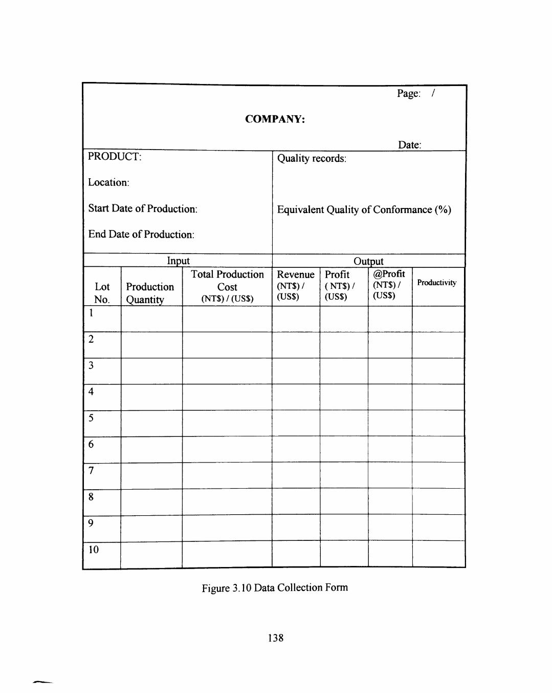
Page: /
COMPANY:
Date: PRODUCT:
Location:
Start Date of Production:
End Date of Production:
Inp
Lot No.
1
2
3
4
5
6
7
8
9
10
Production Quantity
ut Total Production
Cost (NTS) / (US$)
Quality records:
Equivalent Quality ofConformance (%)
Output Revenue (NTS)/ (USS)
Profit (NTS)/ (USS)
@Profit (NTS)/ OJSS)
Productivity
Figure 3.10 Data Collection Form
138
1. Data review and screening
Although data should be collected as accurately as possible, error is
inevitable. It is the responsibility ofthe researcher to pick out these errors
and mistakes according to his knowledge and expertise. Fortunately, this
research chiefly analyzed data by using the concepts of ranks, which
requires only the ordinal scale of measurement, data collected may not
need the accuracy as interval or ratio scales of measurement.
In addition, in this research, a lot of data were converted into
applicable data. For example, quality data was originally collected in
terms of defects per 1000 yards, these data needs to be converted to quality
ofConformance % for this research. Another example was the conversion
from NT$ to US$, this conversion was based on the average exchange rate
during the period of data collection.
2. Data analysis
Only the reviewed and screened data were used for statistical analysis.
Statistical software was used for data analysis. The main technique used
for this analysis was the nonparametric correlation analysis and linear
regression analysis based on ranks. The results ofthe data analysis were
examined and discussed in the following chapters to see whether the
proposed models are appropriate or not.
139
3. Data interpretation
The result ofthe data analysis were interpreted. Regardless ofthe
method used, the interpretation was made under the assumptions and
limitations of this research.
When interpreting data, consistency must be noted. For example,
when quality is proved to be positively correlated with unit profit, this
conclusion cannot be extended to state that quality is positively correlated
with profit. Besides, correlation does not necessarily imply causation, it
might be incorrect to interpret the causation based on correlation analysis.
3.4 Methodological Issues
For any valuable research, the accuracy, effectiveness, precision, bias, and
sufficiency of a research are required. Therefore, a researcher must take into account
the reliability, validity, replicability, bias, and representativeness ofthe research. In
this section, each of these five issues related to the research methodology is
addressed.
3.4.1 Reliability
"Reliability deals with accuracy" indicated by Leedy (1993, p. 42). In other
words reliable research accurately measures what the researcher intends to measure.
140
The issue of reliability in this research mainly results from two aspects: data and tools
(or instruments, machines).
Data reliability is mostly determined by the primary data. The primary data of
this research includes the production cost, revenue, and production quantity collected
by the researcher and the task force in each company. These data were collected
from the accounting systems which also provided these reliable data to management.
There are two types of problems created in the secondary data which may
result in errors in data reliability. One problem is the errors caused in observation or
recording by employees. The other problem is the measurement errors caused by the
unskillful operator. In this research, the problem of data reliability lay mainly in the
errors or mistakes made by the employee due to human error. To prevent, or
eliminate as much as possible, this type of problem of data errors or mistakes, two
solutions were provided. First, any unusual data were picked out when reviewing
collected data. Second, each employee used in the research was approved to assist in
the research due to their level of work competency.
Errors in tool reliability can be attributed to the inacciu-acy of tools,
instruments or machines. Data are the resuhs of measures from these tools (or
instruments, machines). Without correct data, the research results are useless.
Therefore, keeping the tools (or instruments, machines) accurate at all times is
crucial to collecting correct data.
141
Calibration can be regarded as "the quality control of quality control" since it
dominates the data output. The best way to prevent the error in tool reliability caused
by inaccurate tools, instruments, or machines is to make sure that these tools,
instruments, and machines are periodically calibrated to keep them operating
normally. Each company of this research had a calibration schedule, machines,
instruments, or tools were checked having been calibrated on schedule before
collecting data. Errors due to the inaccuracy of machines, instruments, or tools were
eliminated to the minimum extent.
3.4.2 Validity
Leedy (1993) indicates that "Validity is concerned with the soundness, the
effectiveness ofthe measuring instrumenf (p. 40). That is, the validity issue is
concerned yvath whether the measure is really measuring what it is expected to.
According to Leedy, the most common types of validity are: face, criterion, content,
construct, internal, and external validity.
Face validity basically asks two questions: "(1) Is the instnunent measiuing
what it is supposed to measure? (2) Is the sample being measured adequate to be
representative ofthe behavior or trait being measured?" (Leedy, 1993; p. 41). These
questions are similar to the representativeness issue, which is addressed in section
3.4.5. Since this research selected the most representative products (the largest sales
142
volume ofthe company), the research subject was adequately representative ofthe
trait being measured. Therefore, face validity was considered in this research.
Criterion validity employs a second measure to check the accuracy ofthe first
measure. Since accuracy is the main concern of reliability, it was addressed in
section 3.4.1. In addition, group discussion was employed to eliminate the potential
data errors. The check for the accuracy ofthe first measurement was taken into
account.
Content validity is concerned v^th whether the intended factors or situations
are measured. The research method of section 3.2.5 addressed the content validity.
The intended factors were collected and analyzed by the researcher and the task
force, which consisted of experienced engineering representatives, thus content
validity was addressed in this research.
Construct validity deals yvith whether the construct itself is actually measured.
Since this research followed a definite methodology, construct validity is taken into
account.
Internal validity is the "freedom from bias in forming conclusions in view of
the data" (Leedy, 1993; p. 41). Because this research conducted statistical analysis,
the change in the dependent variable was influenced by the independent variable
rather than the research design or the researcher. Therefore, internal validity was
addressed in this research.
143
External validity is related to the generalizability ofthe conclusions drawn
from a sample. Since hypotheses testing of this research were tested based on the
sample, the result of testing undoubtedly possesses external validity because ofthe
trait of statistics. However, the mathematical model developed is limited when
generalized to other cases.
3.4.3 Replicability
Replicability is concerned with the precision of measiu-ement. In theory,
given the same circumstances, research conducted by different researchers on a
specific problem should yield the same results. Replicability is the extent ofthe
consistency; therefore, it is also called repeatability.
Replicability, in essence, does not guarantee that research can achieve what
the researcher intends and expects to determine; however, good research must be
replicable so that other researchers may get identical results. Because this research
specified the research environment, variables, parameters, and definitions, and
followed the research design and methodology, the replicability issue has been taken
into account. Any deviations from the research design has been noted and reported.
^ In statistical terms, mean relates to the accuracy while standard deviation relates to the precision. An accurate mean may not be precise, and vice versa.
144

3.4.4 Bias
Leedy (1993) emphasized that bias is inevitably inherent in all research, and is
usually not perceptible especially in descriptive survey research. Bias often enters the
research design in several ways. First, bias is created through sampling methods
which do not result in representative samples. That is, not all ofthe possible samples
are considered, histead, some portion ofthe population is neglected. For instance,
when sampling from the telephone directory to conduct a survey on the general
consumer's opinion, those consumers who are not listed in the directory are
neglected.
Second, inappropriate interpretation or inference can produce bias. A
researcher may exaggerate an explanation or inference based on the facts available.
For example, based on the results found in a small-sized sample, the researcher may
apply his/her findings to a large population. This creates a problem in the confidence
level in the research.
Third, the researcher's personality can also generate bias. That is, the
subjectivity, preference, intention, and other personality traits may affect data
collection, analysis, research method, and conclusions in the research. For example,
when interviewing subjects, a researcher may spend more time talking to a subject
with whom he/she feels more comfortable, and less time interviewing a subject
whom he/she does not like to talk to. This could possibly distort the facts and hence,
cause the problem of bias.
145
In addition, bias is caused by the order the questions asked. That is, when
asking questions, the order ofthe questions is likely to affect the answers. This
problem is especially significant in interviev^ng and questionnaires. If questions are
not interesting, or are too long, the respondent may lose interest and fail to answer all
questions completely and honestly. Therefore, the answers to latter questions may
not reflect the truth.
Finally, bias may be generated through the wording. That is, some
controversial, arguable, paradoxical, or imdefined words may result in incorrect
answers. For example, if the product quality is not clearly defined, the question, "Do
you think the product quality is good or not?" is very likely to create bias among
different respondents.
Since this research is not descriptive, the problem of bias is not as prevalent
as in qualitative research. However, as Leedy stressed, bias always exists. The
researcher attempted to eliminate the bias as much as possible. This research
followed the statistical principals to avoid the sampling and confidence biases. In
addition, this research employed a task group to assist in data collection, definition,
and measurement to ameliorate any bias by the researcher in establishing these
measures. Finally, the group work reduced the individual personality bias as well as
wording bias.
146
3.4.5 Representativeness
Representativeness deals with the generalizability of research. It may not be
possible to generalize the conclusion of a research project to the similar problems of
other research which is conducted under different circumstances. Each research
project must indicate the extent to which the research may be generalized. In general,
the conclusion of theoretical research is more generalizable than that of a case study
because each case study is, by its nature, bounded by special circumstance. However,
it is not implied that research yvith higher generalizability is more valuable than the
research with lower generalizability.
In this research, the proposed mathematical models and the hypotheses which
state the positive relationships between quality and profit, productivity and profit, and
quality and productivity, can be generalized to manufacturing companies. In
addition, the approach to establish and test the specific models is also generalizable.
The fact that the specific models might not be generalizablly applied to other cases is
acknowledged. However, a specific model can be set up for a specific case by
following the procedures presented in this research.
3.5 Research Constraints
While the limitations described in section 1.3.1 are from a broader viewpoint,
this research still has additional limitations which have not been specifically
mentioned. In fact, it is difficult to list all ofthe limitations since any specific
147
condition of research is a potential limitation. However, several important
limitations of this research in addition to the limitations of sec 1.3.1 must be
addressed.
I Only two products are studied in each case company. Although each
company had many types of products, it was difficult, based on time and
cost constraints, to investigate all of their products.
2. Because the products ofthe XYZ Company were made to stock, its revenue
was estimated by the product of expected selling price and production
quantity. It was likely that a few factors, such as discounts, may affect
revenue.
3. To avoid the influence on the data analysis, all measiu-es in terms of dollars
were applied a fixed exchange rate between the NT$ and US$.
4. Although the same terms were used, e.g., product nonconformance, the
definitions may be different among the companies. Therefore, it is possible
to have a term based on different definitions in different companies.
5. Low product quality levels may invalidate result in the proposed models.
The proposed mathematical models were developed based on the important
assumption that "all quality conformed products can be sold." That is, only
when quality conformance levels meet customer requirements, can all
products be accepted and the manufacturer gains profit from the customer.
148
CHAPTER 4
FIELD STUDY RESULTS, ANALYSIS, AND DISCUSSION
This chapter presents the data collected, analysis ofthe results, and general
discussion. All data presented here were collected in a field study conducted from
June through October of 1996 m Taiwan. Data of ABC Company were collected in
months while data of XYZ Company were in lots. Before starting data collection,
definitions of quality and productivity for separate participating companies were first
determined. Both primary and secondary data are addressed in this chapter. The
primary data include production cost, revenue, and production quantity. The
secondary data consists of profit and productivity, and product quality. These data
were collected, screened, and converted to the desired form of this research.
Figure 4.1 depicts the sequence of this chapter. The task force in each
company assisted the researcher in dealing with the data collection, including primary
and secondary data. This is introduced in section 4.1. Results of data collection are
presented in section 4.2. Based on the results of collected data, hypotheses were
tested to verity the relationships of Quality-Profit, Productivity-Profit, and Quality-
Productivity. This is presented in section 4.3. Model analysis regarding the three
relationships in each company are also presented in section 4.3. Finally, a general
discussion of these relationships are addressed in the last section, section 4.4.
149
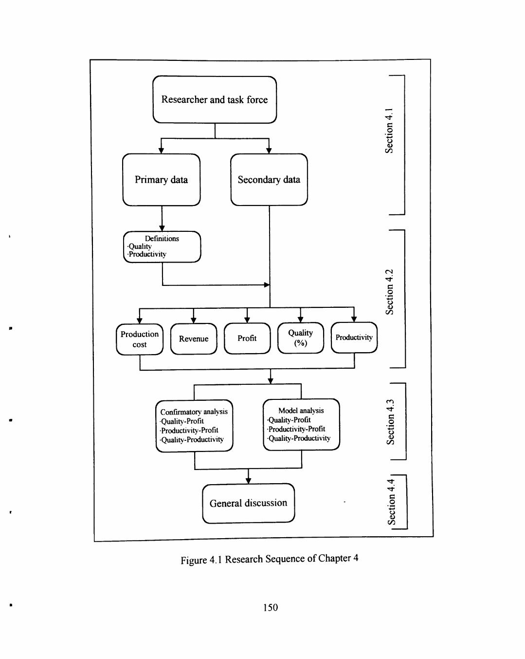
•>v
Researcher and task force
o C/3
Primary data Secondary data
Definitions •Quality •Productivity
r ^ Production
cost Revenue
Z/1
Productivity
I Confirmatory analysis •Quality-Profit •Productivity-Profit •Quality-Productivity
^ Model analysis
•Quality-Profit •Productivity-Profit •Quality-Productivity
cn
c
O
General discussion
C/3
Figure 4.1 Research Sequence of Chapter 4
150
4.1 Introduction
This section introduces company contacts and presents the data collected in
the field study. Subsection 4.1.1 briefly introduces the company contacts in the two
companies used in the research endeavor. Definitions of quality and productivity are
presented in section 4.1.2. Primary data and secondary data are addressed in
subsections 4.1.3 and 4.1.4, respectively.
4.1.1 Company Contacts
In each ofthe two companies of this study, an informal task force was
organized to help the researcher conduct this study. Due to the fact that most data
used in this research are confidential and members ofthe task force are more familiar
with the production, this research needed their assistance. The study was conducted
under the permission ofthe president in each company. All members ofthe task
forces were chosen partially due to their interests in the topic of this research.
Definitions of quality and productivity were discussed together y^th members of task
force. Secondary data were also collected through their aids. In the ABC Company,
an experienced plant manager and two colleagues, his assistant and the QC manager,
ardently supported this research. In the XYZ Company, this research was assisted by
the director of operations and two division managers, manager of manufacturing and
chief of QA.
151

Both companies emphasized that part ofthe data, especially the production
cost and revenue, could be valuable information to their competitors. The researcher
was required not to reveal their company names.
4.1.2 Operation Definition
Operafion definition of this research includes the definitions of quality and
productivity in the two companies (Table 4.1). These definitions were acquired from
group discussion and are used for the selected products of these two companies. The
definitions may not be applicable to other similar products or companies because they
are customer-oriented; and customer needs vary in different products and companies.
Definition of product quality in the ABC Company is completely determined
by the customer orders. For this research, product quality is measured by quality
conformance level (%). In the XYZ Company, products with defects are not allowed
to sell. In other words, the finished products quality must be 100% conformance.
For management purposes, quality must be measured and controlled during the
process. Quality conformance level (%) is used for measuring the product quality
within process.
The definitions ofproductivity in both companies are nearly the same.
However, the total revenue of XYZ company is based on the expected revenue, not
the actual revenue. Actual revenue is difficult to realize imless the products are sold
out, because all products in the XYZ Company are made to stock, actual revenue is
152
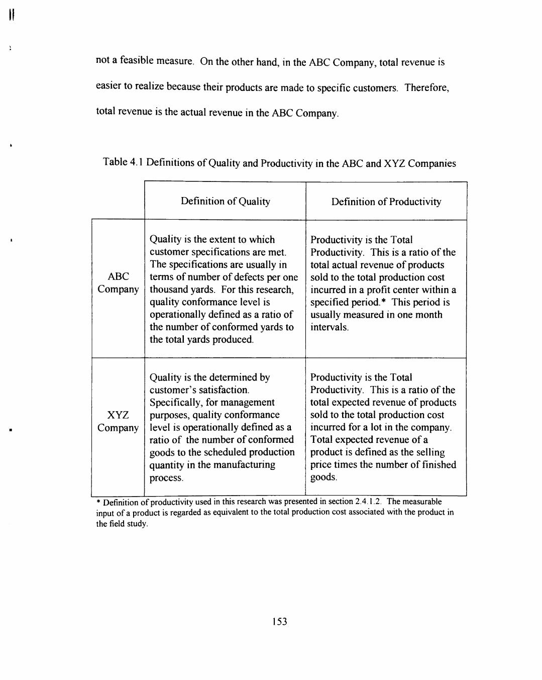
II
not a feasible measure. On the other hand, in the ABC Company, total revenue is
easier to realize because their products are made to specific customers. Therefore,
total revenue is the actual revenue in the ABC Company.
Table 4.1 Definitions of Quality and Productivity in the ABC and XYZ Companies
ABC Company
XYZ Company
Definition of Quality
Quality is the extent to which customer specifications are met. The specifications are usually in terms of number of defects per one thousand yards. For this research, quality conformance level is operationally defined as a ratio of the number of conformed yards to the total yards produced.
Quality is the determined by customer's satisfaction. Specifically, for management purposes, quality conformance level is operationally defined as a ratio of the number of conformed goods to the scheduled production quantity in the manufacturing process.
Definition of Productivity
Productivity is the Total Productivity. This is a ratio ofthe total actual revenue of products sold to the total production cost incurred in a profit center within a specified period.* This period is usually measured in one month intervals.
Productivity is the Total Productivity. This is a ratio of the total expected revenue of products sold to the total production cost inciuTcd for a lot in the company. Total expected revenue of a product is defined as the selling price times the number of finished goods.
* Definition ofproductivity used in this research was presented in section 2 4.1.2. The measurable input of a product is regarded as equivalent to the total production cost associated with the product in the field study.
153
4.1.3 Primary Data Collected
Three major primary data required for this study were collected in each
company. These data were production cost, revenue, and production quantity. Other
minor data, lot number, were also recorded. Lot number indicates the sequence of
production lots in the XYZ Company. According to the lot sequence, data were
tested for independence of time.
Production cost and revenue data were specially essential to this research.
The analysis of this research concentrated on the profit-based relationships.
According to the definition of this research, profit is the difference between revenue
and production cost. That is, profit data were determined from these two types of
data. These production cost and revenue data were collected by the assistance from
the accoimting department in each company.
In addition to the production cost and total revenue, production quantity was
also important to this research. Because this research relates quality and productivity
based on unit profit, which is an average profit, production quantity were collected
for calculating the unit profit. In each company, the calculation of unit profit
assumed each product in the same lot or month has equal contribution to the profit.
4.1.4 Secondary Data Collected
Three secondary data were collected. Profit data were easily secured by
subtracting production cost from total revenue. Original quality data were collected
154
and transformed into desired conformance level(%). The inspection points that
identify defects in the products of each company are listed in Appendix B. In both
companies, quality was not expressed in conformance level (in ABC, it is the number
of defects per 1000 yards while in XYZ, the finished product must be 100%
conformed). For the purpose of comparing variables in this research, all quality data
were converted to conformance level (%). These quality data were attained by
converting the available quality records into the desired % (see the definitions of
quality for each company in the previous subsection 4.1.2).
Productivity data were acquired through the calculation of revenue to
production cost. In both companies, productivity was defined as the ratio of revenue
to production cost. Like profit, productivity data were also easily calculated when
both production cost and revenue data were available.
The monetary unit used in the remaining sections is US dollars. Since the two
companies are in Taiwan, the original costs, revenue, and profit are all in New
Taiwan Dollars (NT$). During the studying period, the average exchange rate
between US$ and NT$ was close to 1: 27.5. ' For this research, all monetary data
collected in NT$ were converted into USS according to this average exchange rate.
• According to the China Times of Taiwan, the exchange rate between USS and NTS fluctuated approximately between 27.3 to 27.7 during the studying period fi-om June to October of 1996. Therefore, the average exchange rate 27.5 was used.
155
All the results of collected data are presented in the next section. Based on
these data, a statistical analysis and general discussion are conducted in the following
sections 4.3 and 4.4.
4.2 Results of Collected Data
This section presents the results of data collected in the field study. Sections
4.2.1 through 4.2.5 present these data which are summarized based on separate
products in each company. The data collected in the ABC Company were measured
in months while in the XYZ Company, they were measured in lots. This was because
the production process in ABC Company was flow-type, it adopted a process costing
system. On the other hand, the XYZ Company made products to stock and produces
lot by lot, so the batch costing system was used.
4.2.1 Production Cost Data
Tables 4.2 and 4.3 show the production cost data collected in the three
factories. A, B, and C of ABC Company for gingham and piece-dyed fabric
respectively. The number, in thousands of yards, in the last column, stands for the
production quantity of each month. Tables 4.4 and 4.5 list the production cost data
collected in the XYZ Company.
156
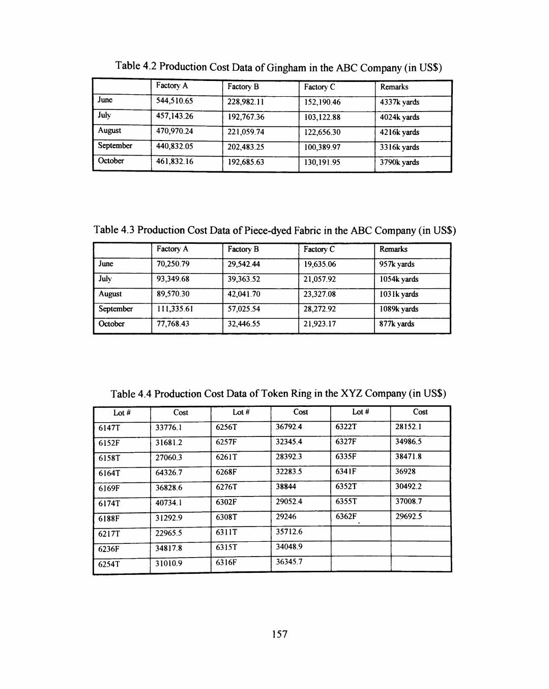
Table 4.2 Production Cost Data of Gingham in the ABC Company (in US$)
June
July
August
September
October
Factory A
544,510.65
457,143.26
470,970.24
440,832.05
461,832.16
Factory B
228,982.11
192,767.36
221,059.74
202,483.25
192,685.63
Factory C
152,190.46
103,122.88
122,656.30
100,389.97
130,191.95
Remarks
4337k yards
4024k yards
4216k yards
3316k yards
3790k yards
Table 4.3 Production Cost Data of Piece-dyed Fabric in the ABC Company (in USS)
June
July
August
September
October
Factory A
70,250.79
93,349.68
89,570.30
111,335.61
77,768.43
Factory B
29,542.44
39,363.52
42,041.70
57,025.54
32,446.55
Factory C
19,635.06
21,057.92
23,327.08
28,272.92
21,923.17
Remarks
957k yards
1054k yards
103 Ik yards
1089k yards
877k yards
Table 4.4 Production Cost Data of Token Ring in the XYZ Company (in USS)
Lot#
6147T
6152F
6158T
6164T
6169F
61741
6188F
6217T
6236F
6254T
Cost
33776.1
31681.2
27060.3
64326.7
36828.6
40734.1
31292.9
22965.5
34817.8
31010.9
Lot#
6256T
6257F
626 IT
6268F
6276T
6302F
6308T
631IT
6315T
6316F
Cost
36792.4
32345.4
28392.3
32283.5
38844
29052.4
29246
35712.6
34048.9
36345.7
Lot#
6322T
6327F
6335F
634 IF
6352T
6355T
6362F
Cost
28152.1
34986.5
38471.8
36928
30492.2
37008.7
29692.5
157
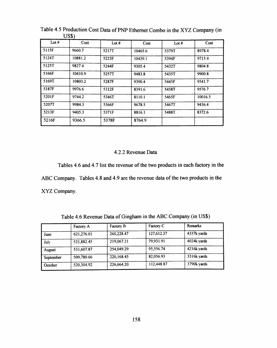
Table 4.5 Production Cost Data of PNP Ethernet Combo in the XYZ Company (in USS)
Lot#
5115F
5124T
5125T
5166F
5169T
5187F
520 IF
5207T
5213F
5216F
Cost
9660.7
10881.2
9827 4
10410.9
10803.2
9976.6
9744.2
9984.3
9405.3
9366.5
Lot#
5217T
5223F
5244F
5257T
5287F
5312F
5346T
5366F
5371F
5378F
Cost
10465.6
10439.1
9305.4
9483.8
9390.4
8391.6
8110.1
9678.5
8816.1
8764.9
Lot#
5379T
5394F
5432T
5435T
5445F
5458T
5465F
5467T
5488T
Cost
8978.4
9715.4
9804.8
9900.8
9541.7
9576.7
10016.5
9436.4
8372.6
4.2.2 Revenue Data
Tables 4.6 and 4.7 list the revenue ofthe two products in each factory in the
ABC Company. Tables 4.8 and 4.9 are the revenue data ofthe two products in the
XYZ Company.
Table 4.6 Revenue Data of Gingham in the ABC Company (in USS)
June
Juh
August
September
October
Factory A
621,276.01
521,882.45
531,607.87
509,780.66
520,304.92
Factory B
260,228.47
219,067.21
254,049.29
220,168.45
226,664.20
Factory C
127,612.37
79,931.91
95,556.74
82,056.93
112,448.87
Remarks
4337k yards
4024k yards
4216k yards
3316k yards
3790k yards
158
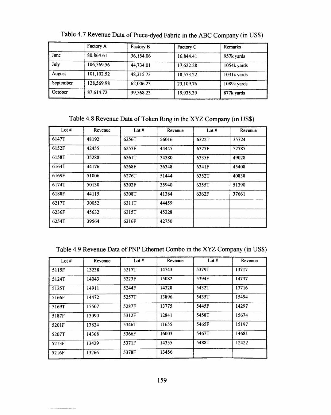
Table 4.7 Revenue Data of Piece-dyed Fabric in the ABC Company (in USS)
June
July
August
September
October
Factory A
80,864.61
106,569.56
101,102.52
128,569.98
87,614.72
Factory B
36,154.06
44,734.01
48,315.73
62,006.23
39,568.23
Factory C
16,844.41
17,622.28
18,573.22
23,109.76
19,935.39
Remarks
957k yards
1054k yards
103 Ik yards
1089k yards
877k yards
Table 4.8 Revenue Data of Token Ring in the XYZ Company (in USS)
Lot#
6147T
6152F
6158T
6164T
6169F
6174T
6188F
6217T
6236F
6254T
Revenue
48192
42455
35288
44176
51006
50130
44115
30052
45632
39564
Lot#
6256T
6257F
626 IT
6268F
6276T
6302F
6308T
631 IT
6315T
6316F
Revenue
56016
44445
34380
36348
51444
35940
41384
44459
45328
42750
Lot#
6322T
6327F
6335F
634 IF
6352T
6355T
6362F
Revenue
35724
52785
49028
45408
40838
51390
37661
Table 4.9 Revenue Data of PNP Ethernet Combo in the XYZ Company (in USS)
Lot#
5115F
5124T
5125T
5166F
5169T
5187F
5201F
5207T
5213F
5216F
Revenue
13238
14043
14911
14472
15507
13090
13824
14368
13429
13266
Lot#
5217T
5223F
5244F
5257T
5287F
5312F
5346T
5366F
5371F
5378F
Revenue
14743
15082
14328
13896
13775
12841
11655
16003
14355
13456
Lot#
5379T
5394F
5432T
5435T
5445F
5458T
5465F
5467T
5488T
Revenue
13717
14737
13716
15494
14297
15674
15197
14681
12422
159
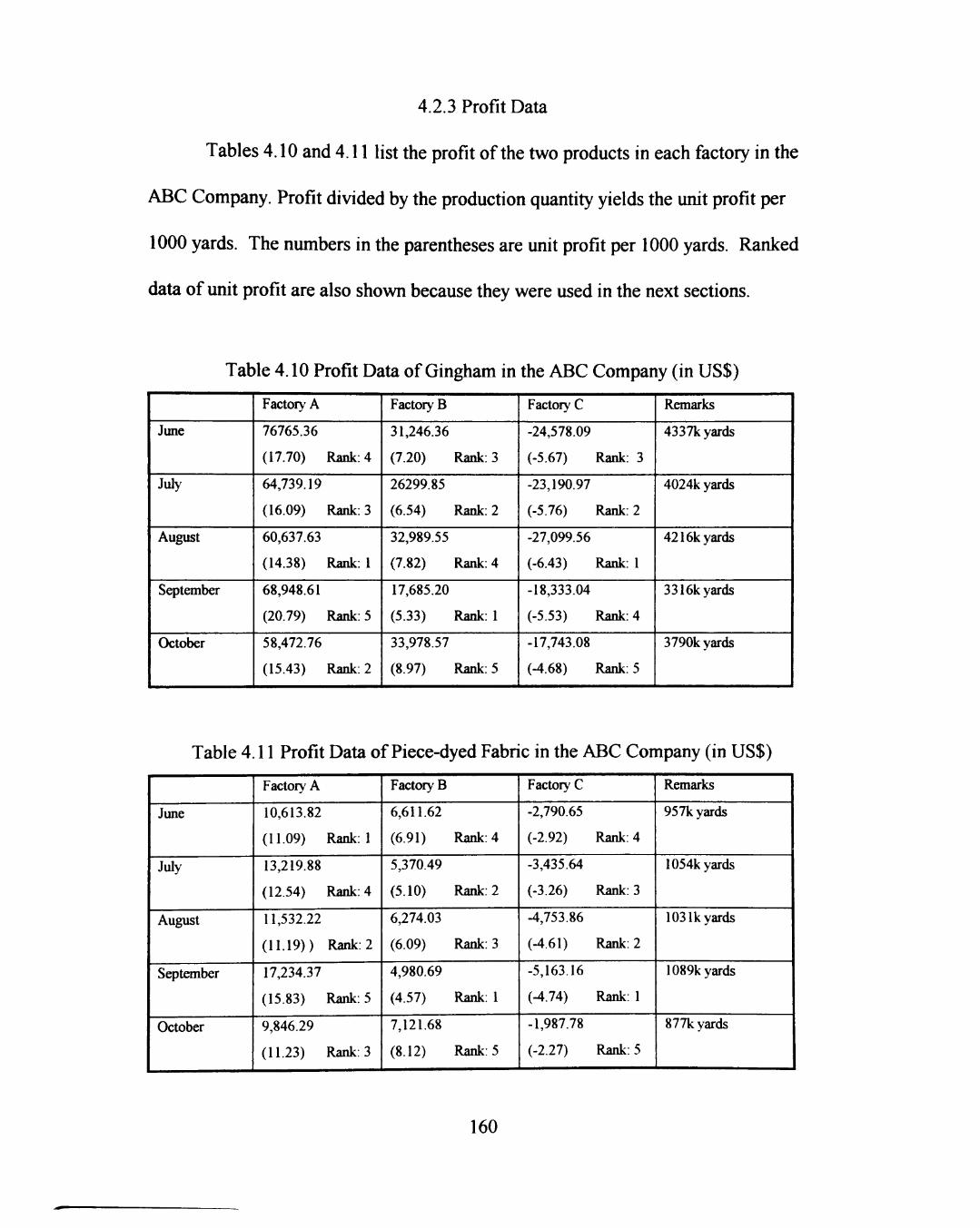
4.2.3 Profit Data
Tables 4.10 and 4.11 list the profit ofthe two products in each factory in the
ABC Company. Profit divided by the production quantity yields the unit profit per
1000 yards. The numbers in the parentheses are unit profit per 1000 yards. Ranked
data of unit profit are also shown because they were used in the next sections.
Table 4.10 Profit Data of Gingham in the ABC Company (in USS)
June
July
August
September
October
Factory A
76765.36
(17.70) Rank: 4
64,739.19
(16.09) Rank: 3
60,637.63
(14.38) Rank: 1
68,948.61
(20.79) Rank: 5
58,472.76
(15.43) Rank: 2
Factory B
31,246.36
(7.20) Rank: 3
26299.85
(6.54) Rank: 2
32,989.55
(7.82) Rank: 4
17,685.20
(5.33) Rank: 1
33,978.57
(8.97) Rank: 5
Factory C
-24,578.09
(-5.67) Rank: 3
-23,190.97
(-5.76) Rank: 2
-27,099.56
(-6.43) Rank: 1
-18,333.04
(-5.53) Rank: 4
-17,743.08
(-4.68) Rank: 5
Remarks
4337k yards
4024k yards
4216k yards
3316k yards
3790k yards
Table 4.11 Profit Data of Piece-dyed Fabric in the ABC Company (in USS)
June
July
August
September
October
Factory A
10,613.82
(11.09) Rank: 1
13,219.88
(12.54) Rank: 4
11,532.22
(11.19)) Rank: 2
17,234.37
(15.83) Rank: 5
9,846.29
(11.23) Rank: 3
Factory B
6,611.62
(6.91)
5,370.49
(5.10)
6,274.03
(6.09)
4,980.69
(4.57)
7,121.68
(8.12)
Rank: 4
Rank: 2
Rank: 3
Rank: 1
Rank: 5
Factory C
-2,790.65
(-2.92)
-3,435.64
(-3.26)
-4,753.86
(-4.61)
-5,163.16
(-4.74)
-1,987.78
(-2.27)
Rank: 4
Rank: 3
Rank: 2
Rank: 1
Rank: 5
Remarks
957k yards
1054k yards
103 Ik yards
1089k yards
877k yards
160
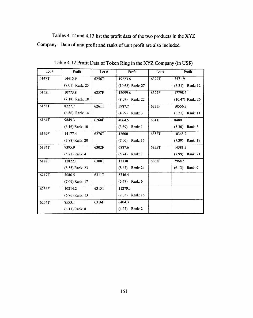
Tables 4.12 and 4.13 list the profit data ofthe two products in the XYZ
Company. Data of unit profit and ranks of unit profit are also included.
Table 4.12 Profit Data of Token Ring in the XYZ Company (in USS)
Lot#
6147T
6152F
6158T
6164T
6169F
6174T
6188F
6217T
6236F
6254T
Profit
14415.9
(9.01) Rank: 25
10773.8
(7.18) Rank: 18
8227.7
(6.86) Rank: 14
9849.3
(6.16) Rank: 10
14177.4
(7.88) Rank: 20
9395.9
(5.22) Rank: 4
12822.1
(8.55) Rank: 23
7086.5
(7.09) Rank: 17
10814.2
(6.76) Rank: 13
8553.1
(6.11) Rank: 8
Lot#
6256T
6257F
626 IT
6268F
6276T
6302F
6308T
631 IT
6315T
6316F
Profit
19223.6
(10.68) Rank: 27
12099.6
(8.07) Rank: 22
5987.7
(4.99) Rank: 3
4064.5
(3.39) Rank: 1
12600
(7.00) Rank: 15
6887.6
(5.74) Rank: 7
12138
(8.67) Rank: 24
8746.4
(5.47) Rank: 6
11279.1
(7.05) Rank: 16
6404.3
(4.27) Rank: 2
Lot#
6322T
6327F
6335F
634 IF
6352T
6355T
6362F
Profit
7571.9
(6.31) Rank: 12
17798.5
(10.47) Rank: 26
10556.2
(6.21) Rank: 11
8480
(5.30) Rank: 5
10345.2
(7.39) Rank: 19
14381.3
(7.99) Rank: 21
7968.5
(6.13) Rank: 9
161
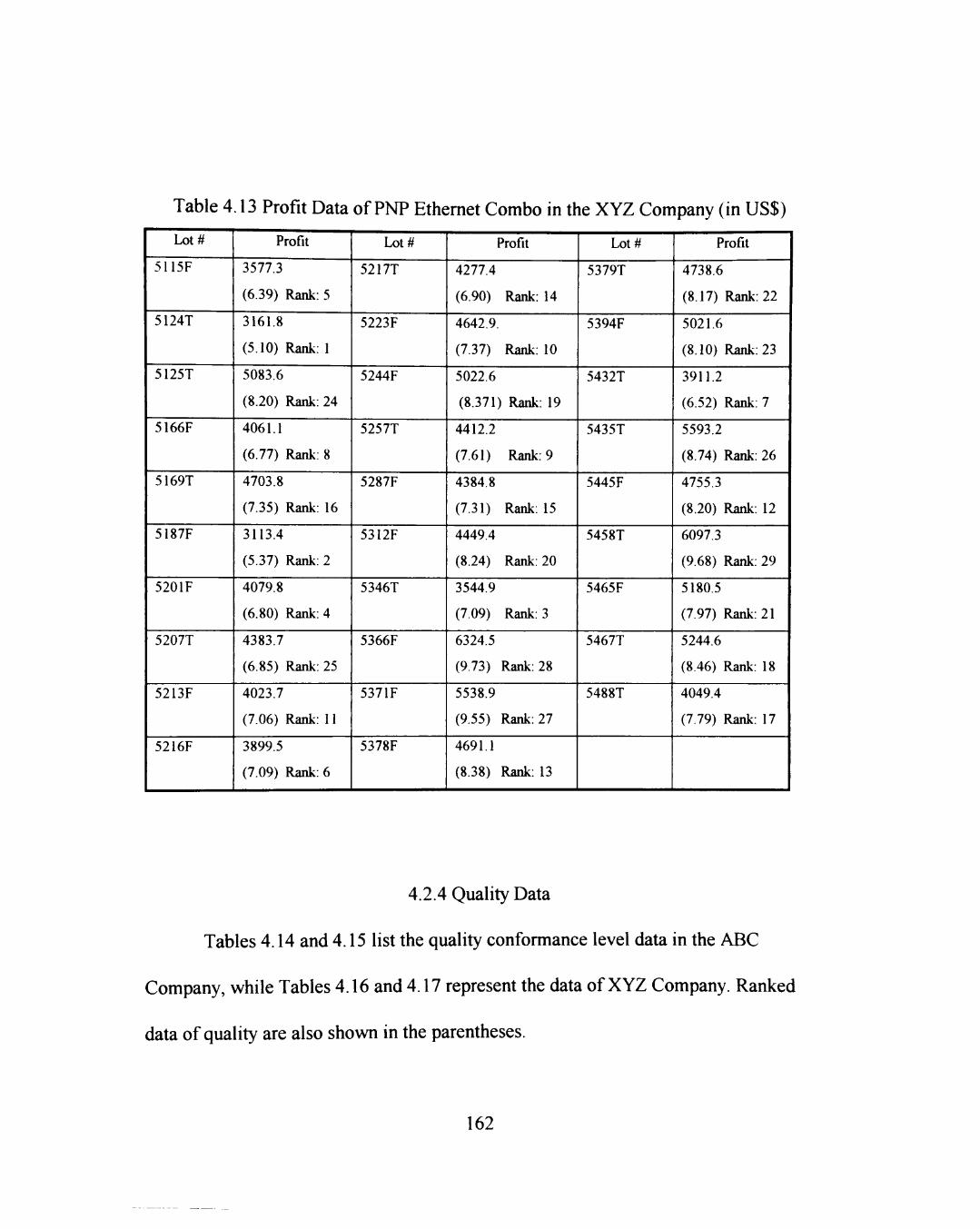
Table 4.13 Profit Data of PNP Ethernet Combo in the XYZ Company (in USS)
Lot#
5115F
5124T
5125T
5166F
5169T
5187F
5201F
5207T
5213F
5216F
Profit
3577.3
(6.39) Rank: 5
3161.8
(5.10) Rank: 1
5083.6
(8.20) Rank: 24
4061.1
(6.77) Rank: 8
4703.8
(7.35) Rank: 16
3113.4
(5.37) Rank: 2
4079.8
(6.80) Rank: 4
4383.7
(6.85) Rank: 25
4023.7
(7.06) Rank: 11
3899.5
(7.09) Rank: 6
Lot#
5217T
5223F
5244F
5257T
5287F
5312F
5346T
5366F
5371F
5378F
Profit
4277.4
(6.90) Rank: 14
4642.9.
(7.37) Rank: 10
5022.6
(8.371) Rank: 19
4412.2
(7.61) Rank: 9
4384.8
(7.31) Rank: 15
4449.4
(8.24) Rank: 20
3544.9
(7.09) Rank: 3
6324.5
(9.73) Rank: 28
5538.9
(9.55) Rank: 27
4691.1
(8.38) Rank: 13
Lot#
5379T
5394F
5432T
5435T
5445F
5458T
5465F
5467T
5488T
Profit
4738.6
(8.17) Rank: 22
5021.6
(8.10) Rank: 23
3911.2
(6.52) Rank: 7
5593.2
(8.74) Rank: 26
4755.3
(8.20) Rank: 12
6097.3
(9.68) Rank: 29
5180.5
(7.97) Rank: 21
5244.6
(8.46) Rank: 18
4049.4
(7.79) Rank: 17
4.2.4 Quality Data
Tables 4.14 and 4.15 list the quality conformance level data in the ABC
Company, while Tables 4.16 and 4.17 represent the data of XYZ Company. Ranked
data of quality are also shown in the parentheses.
162
Table 4.14 Quality Conformance Level of Gingham in
June
July
August
September
October
Factory A
97.80% (4)
97.28% (3)
96.33% (1)
97.83% (5)
96.50% (2)
Factory B
97.86% (3)
97.65% (2)
98.16% (4)
97.50% (1)
98.64% (5)
Facton, C
96.83% (3)
96.80% (2)
96.35% (1)
97.62% (4)
98.74% (5)
The values in parentheses ( ) located in each cell indicate the respective rank ofthe field data in that cell.
Table 4.15 Quality Conformance Level of Piece-dyed Fabric in the ABC Company (in USS)*
June
JuK
August
September
October
Factory A
97.91% (4)
97.86% (3)
97.51% (1)
98.73% (5)
97.55% (2)
Factory B
98.32% (3)
98.1% (2)
98.53% (4)
97.50% (1)
98.64% (5)
Factors C
97.78% (4)
97.18% (3)
96.53% (2)
96.09% (1)
98.08% (5)
* The values in parentheses ( ) located in each cell indicate the respective rank ofthe field data in that cell.
Table 4.16 Quality Conformance Level of Token Ring in the XYZ Company (in USS) Lot#
6147T
6152F
6158T
6164T
6169F
6174T
6188F
6217T
6236F
6254T
Quality
96.88% (25)
95.67% (18)
93.83% (9)
93.94% (12.5)
96.00% (21)
92.72% (4)
96.53% (23)
95.20% (17)
94.06% (14)
93.64% (8)
Lot#
6256T
6257F
626 IT
6268F
6276T
6302F
6308T
6311T
6315T
6316F
Quality
96.94% (26)
96.13% (22)
92.33% (2.5)
92.08% (1)
94.16% (15)
93.08% (7)
96.79% (24)
92.94% (6)
94.56% (16)
92.33% (2.5)
Lot#
6322T
6327F
6335F
634 IF
6352T
6355T
6362F
Quality
93.92% (11)
97.06% (27)
93.94% (12.5)
92.81% (5)
95.79% (19)
95.94% (20)
93.85% (10)
* The values in parentheses ( ) located in each cell indicate the respective rank ofthe field data in that cell.
163
Table 4.17 Quality Conformance Level of PNP Ethernet Combo in the XYZ Company (in USS)*
Lot#
5115F
5124T
5125T
5166F
5169T
5187F
520 IF
5207T
5213F
5216F
Quality
91.43% (3)
90.32% (1)
95.48% (26)
92.50% (5)
94.38% (13)
91.03% (2)
93.17% (7)
93.44% (8)
92.98% (6)
93.64% (9)
Lot#
5217T
5223F
5244F
5257T
5287F
5312F
5346T
5366F
5371F
5378F
Quality
93.87% (10)
94.440/0 (14)
95.50% (27)
94.48% (15)
94.17% (11)
95.19% (22)
94.20% (12)
95.38% (25)
95.69% (28)
95.18% (21)
Lot#
5379T
5394F
5432T
5435T
5445F
5458T
5465F
5467T
5488T
Quality
94.83% (18)
94.84% (19)
91.50% (4)
95.31% (23)
95.17% (20)
95.87% (29)
94.77% (17)
95.32% (24)
94.62% (16)
* The values cell.
in parentheses ( ) located in each cell indicate the respective rank ofthe field data in that
4.2.5 Productivity Data
Tables 4.18 through 4.21 are the productivity data ofthe two companies.
Niunbers in the parentheses are the ranks ofproductivity.
Table 4.18 Productivity Data of Gingham in the ABC Company (in USS)"
June
July
August
September
October
Factory A
114.10% (3)
114.16% (4)
112.88% (2)
115.64% (5)
112.66% (1)
Factory B
113.65% (3)
113.64% (2)
114.92% (4)
108.73% (1)
117.63% (5)
Factory C
83.85% (4)
77.51% (1)
77.91% (2)
81.74% (3)
86.37% (5)
* The values in parentheses ( ) located in each cell indicate the respective rank ofthe field data in that cell.
164
Table 4.19 Productivity Data of Piece-dyed Fabric in tv»p. ARr r-r tvi o T, ,« T TQC\*
June
July
August
September
October
Factory A
115.11% (4)
114.16% (3)
112.88% (2)
115.48% (5)
112.66% (1)
Factory B
122.38% (5)
113.64% (2)
114.92% (3)
108.73% (1)
121.95% (4)
Factory C
85.79% (4)
83.68% (3)
79.62% (1)
81.74% (2)
90.93% (5)
* The values in parentheses ( ) located in each cell indicate the respective rank ofthe field data in that cell.
Table 4.20 Productivity Data of Token Ring in the XYZ Company (in USS)* Lot#
6147T
6152F
6158T
6164T
6169F
6174T
6188F
6217T
6236F
6254T
Productivity
142.68% (25)
134.01% (19)
130.41% (13)
128.69% (12)
138.50% (21)
123.07% (5)
140.97% (23)
130.86% (14)
131.06% (15)
127.58% (11)
Lot#
6256T
6257F
626 IT
6268F
6276T
6302F
6308T
6311T
6315T
6316F
Productivity
152.25% (27)
137.41% (20)
121.09% (3)
112.59% (1)
132.44% (16)
123.71% (6)
141.50% (24)
124.49% (7)
133.13% (17)
117.62% (2)
Lot#
6322T
6327F
6335F
6341F
6352T
6355T
6362F
Productivity
126.90% (9)
150.87% (26)
127.44% (10)
122.96% (4)
133.93% (18)
138.86% (22)
126.84% (8)
* The values in parentheses ( ) located in each cell indicate the respective rank ofthe field data in that cell.
Table 4.21 Productivity Data of PNP Ethernet Combo in the XYZ Company (in USS)* Lot#
5115F
5124T
5125T
5166F
5169T
5187F
520 IF
5207T
5213F
5216F
Productivity
137.03% (3)
129.06% (1)
151.73% (20)
139.01% (4)
143.54% (10)
131.21% (2)
141.87% (8)
143.91% (12)
142.78% (9)
141.63% (7)
Lot#
52I7T
5223F
5244F
5257T
5287F
5312F
5346T
5366F
5371F
5378T
Productivity
140.87% (6)
144.48% (13)
153.98% (24)
146.52% (14)
146.69% (15)
153.02% (22)
143.71% (11)
165.35% (29)
162.83% (27)
153.52% (23)
Lot#
5379T
5394F
5432T
5435T
5445F
5458T
5465F
5467T
5488T
Productivity
152.78% (21)
151.69% (18)
139.90% (5)
156.50% (26)
149.84% (17)
163.67% (28)
151.72% (19)
155.58% (25)
148.36% (16)
* The values in parentheses ( ) located in each cell indicate the respective rank ofthe field data in that cell.
165
4.3 Data Analysis
Data analysis in this section is divided into two parts: confirmatory analysis
and model analysis. The former is to test the collected data to confirm the alternative
hypotheses proposed in Chapter 3. The latter identifies the models and assesses the
aptness of models for the studied companies. Statistical approaches, especially the
nonparametric correlation analysis and regression analysis, are used throughout this
section. Results of analysis are all summarized with tables.
4.3.1 Confirmatory Analysis
This section deals with the hypotheses tests mentioned in Figures 3.1 and 3.2
of section 3.2.3. The purpose of these tests is to confirm the positive Quality-Profit,
Productivity-Profit, and Quality-Productivity relationships in the studied
manufacturing environments. Since profit is highly dependent on the sales quantity,
unit profit is more meaningful to be used to compare with quality conformance level
and productivity.
The method of this confirmatory analysis is first introduced in subsection
4.3.1.1. According to this method, hypotheses are tested in the order of Quality-
Profit, Productivity-Profit, and Quality-Productivity relationships in subsections
4.3.1.2, 4.3.1.3, and 4.3.1.4, respectively.
166
4.3.1.1 Method of Analysis
The hypotheses presented in Figures 3.1 and 3.2 were tested by correlation
analysis. Because quality conformance level has different meanings to different
products, factories, and companies, rank correlation analysis was used. There are a
couple of methods developed for the computation of rank correlation, the most
commonly used measure. Spearman's Rho, was used to calculate the rank correlation
coefficient.
Based on the rank correlation coefficients calculated for various products,
factories, and companies, hypotheses were tested and conclusions were drawn.
Because the purpose of this subsection, section 4.3.1, is to test the positive correlation
of Quality-Profit, Productivity-Profit, and Quality-Productivity relationships, one-
tailed test was adopted.
After obtaining conclusions from hypotheses tests for all products, factories,
and companies, the confidence intervals ofthe correlation coefficients were
estimated to see the degree these variables correlate with each other. These intervals
reveal the smallest correlation coefficients in each relationships.
Since rank correlation analysis is a distribution-fi-ee approach, it is not
necessary to assume a distribution the population is subject to. However, when using
Spearman's Rho method for analysis, there are basic assumptions:
1. Data samples are random samples.
2. Data must be paired data.
167
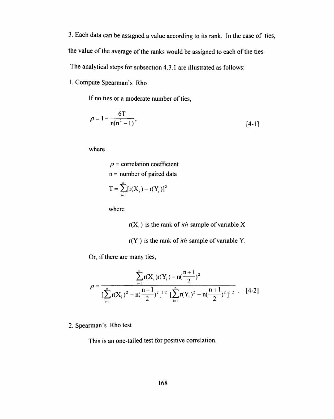
3. Each data can be assigned a value according to its rank. In the case of ties,
the value ofthe average ofthe ranks would be assigned to each ofthe ties.
The analytical steps for subsection 4.3.1 are illustrated as follows:
I. Compute Spearman's Rho
If no ties or a moderate number of ties,
6T p=\-
n(n^- l ) ' [4-1]
where
p = correlation coefficient
n = number of paired data
T=Z[r(X,)-r(Y,)r i = l
where
r(Xi) is the rank of ith sample of variable X
r(Y,) is the rank of ith sample of variable Y.
Or, if there are many ties,
^ n+1 , Zr(X.)r(Y.)-n(-—)^ 1=1 ±
^ ~ x^ , n-i-1 , , , v^ , n + 1 , , , 14-21 [ £ r ( X . ) ^ - n ( ^ - ) ^ ] ' ^ [Er(Y.)^-n(—-)^] '^ ^ ^
1=1 ^ 1=1 ^
2. Spearman's Rho test
This is an one-tailed test for positive correlation.
168
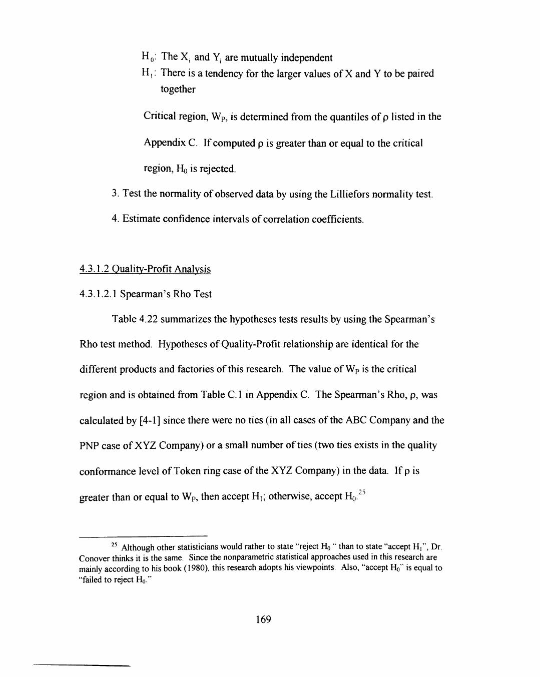
HQ: The Xj and Yj are mutually independent
H,: There is a tendency for the larger values of X and Y to be paired
together
Crifical region, Wp, is determined from the quantiles of p listed in the
Appendix C. If computed p is greater than or equal to the critical
region, HQ is rejected.
3. Test the normality of observed data by using the Lilliefors normality test.
4. Estimate confidence intervals of correlation coefficients.
4.3.1.2 Quality-Profit Analysis
4.3.1.2.1 Spearman's Rho Test
Table 4.22 summarizes the hypotheses tests results by using the Spearman's
Rho test method. Hypotheses of Quality-Profit relationship are identical for the
different products and factories of this research. The value of Wp is the critical
region and is obtained from Table C. 1 in Appendix C. The Spearman's Rho, p, was
calculated by [4-1] since there were no ties (in all cases ofthe ABC Company and the
PNP case of XYZ Company) or a small nimiber of ties (two ties exists in the quality
conformance level of Token ring case ofthe XYZ Company) in the data. If p is
greater than or equal to Wp, then accept Hi; otherwise, accept HQ. ^
^' Although other statisticians would rather to state "reject Ho " than to state "accept Hi", Dr Conover thinks it is the same. Since the nonparametric statistical approaches used in this research are mainly according to his book (1980), this research adopts his viewpoints. Also, "accept HQ" is equal to "failed to reject HQ."
169
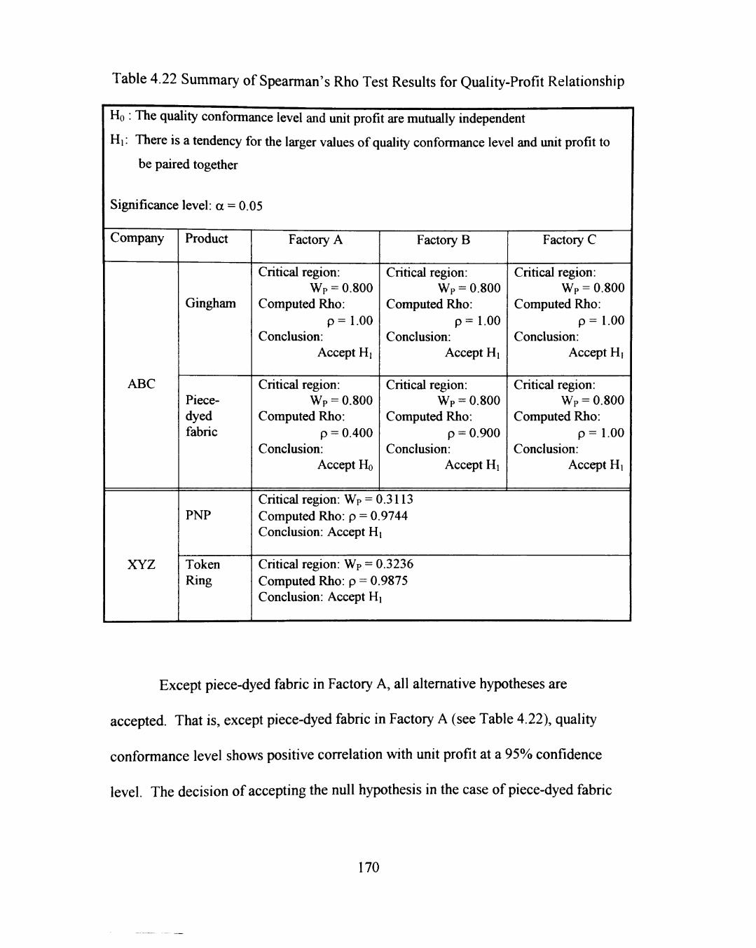
Table 4.22 Summary of Spearman's Rho Test Resuhs for Quality-Profit Relationship
Ho: The quality conformance level and unit profit are muUially independent
HI ! There is a tendency for the larger values of quality conformance level and unit profit to
be paired together
Significance level: a = 0.05
Company
ABC
XYZ
Product
Gingham
Piece-dyed fabric
PNP
Token Ring
Factory A
Critical region: Wp = 0.800
Computed Rho: p=1.00
Conclusion: Accept Hi
Critical region: Wp = 0.800
Computed Rho: p = 0.400
Conclusion: Accept HO
Factory B
Critical region: Wp = 0.800
Computed Rho: p = 1.00
Conclusion: Accept Hi
Critical region: Wp = 0.800
Computed Rho: p = 0.900
Conclusion: Accept Hi
Factory C
Critical region: Wp = 0.800
Computed Rho: p = 1.00
Conclusion: Accept Hi
Critical region: Wp = 0.800
Computed Rho: p = 1.00
Conclusion: Accept Hi
Critical region: Wp = 0.3113 Computed Rho: p = 0.9744 Conclusion: Accept Hi
Critical region: Wp = 0.3236 Computed Rho: p = 0.9875 Conclusion: Accept Hi
Except piece-dyed fabric in Factory A, all alternative hypotheses are
accepted. That is, except piece-dyed fabric in Factory A (see Table 4.22), quality
conformance level shows positive correlation with unit profit at a 95% confidence
level. The decision of accepting the null hypothesis in the case of piece-dyed fabric
170
in Factory A does not mean that HQ is true. It just indicates that Ho has not been
proven to be false. That is, although the conclusion in the case of piece-dyed fabric
in Factory A is to accept HQ, it does not mean that its quality conformance level does
not correlate with unit profit.
4.3.1.2.2 Normality Test
The results ofthe Lilliefors normality test for the sample data of quality and
imit profit are shown in the Appendix D, Figures D. 1 through D.8. All figures show
that, at a 95% confidence level, the observed data subject to normality. Based on the
results, the confidence interval of correlation coefficient of Quality-Profit
relationship can be estimated.
4.3.1.2.3 Estimation of Confidence Interval of Correlation Coefficient
Since the paired data of (Q, Pu) in all cases are shown to be normally
distributed, an estimated confidence interval ofthe eight Spearman's Rhos (shown in
Table 4.22) can be obtained. Due to the fact that the standard deviation ofthe
population is unknown and sample size is small, the following formula (based on
Montgomery, 1991) is used to estimate the confidence interval of correlation
coefficient ofthe population:
p - , „ „ ^ < ^ < p + . . . ^ [4-3]
171
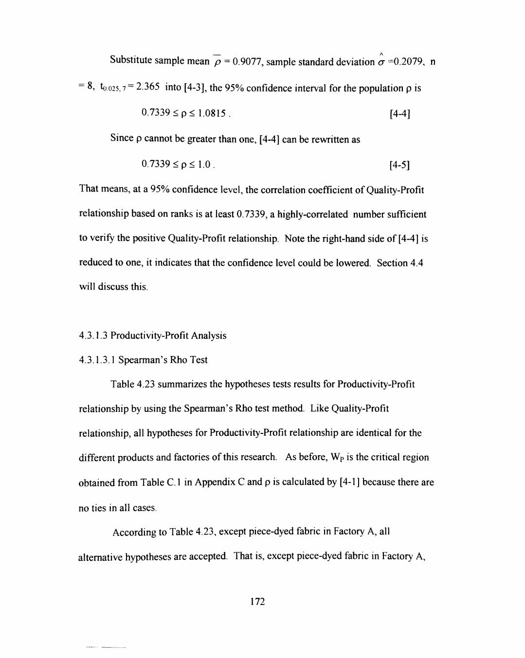
Substitute sample mean p = 0.9077, sample standard deviation G =^2^1^. n
" 8, to 025,7 = 2.365 into [4-3], the 95% confidence interval for the population p is
0.7339 < p < 1.0815. [4-4]
Since p cannot be greater than one, [4-4] can be rewritten as
0.7339<p<1.0. [4-5]
That means, at a 95% confidence level, the correlation coefficient of Quality-Profit
relationship based on ranks is at least 0.7339, a highly-correlated number sufficient
to verify the positive Quality-Profit relationship. Note the right-hand side of [4-4] is
reduced to one, it indicates that the confidence level could be lowered. Section 4.4
will discuss this.
4.3.1.3 Productivity-Profit Analysis
4.3.1.3.1 Spearman's Rho Test
Table 4.23 summarizes the hypotheses tests results for Productivity-Profit
relationship by using the Spearman's Rho test method. Like Quality-Profit
relationship, all hypotheses for Productivity-Profit relationship are identical for the
different products and factories of this research. As before, Wp is the critical region
obtained from Table C. 1 in Appendix C and p is calculated by [4-1] because there are
no ties in all cases.
According to Table 4.23, except piece-dyed fabric in Factory A, all
alternative hypotheses are accepted. That is, except piece-dyed fabric in Factory A,
172
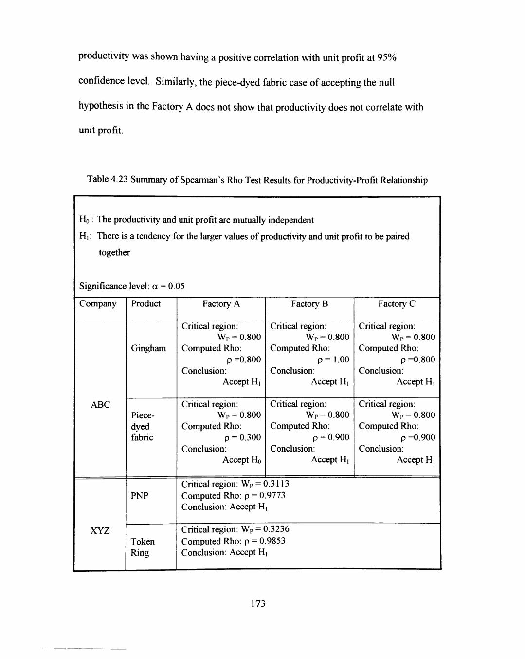
productivity was shown having a positive correlation with unit profit at 95%
confidence level. Similariy, the piece-dyed fabric case of accepting the null
hypothesis in the Factory A does not show that productivity does not correlate with
unit profit.
Table 4.23 Summary of Spearman's Rho Test Results for Productivity-Profit Relationship
Ho : The productivity and unit profit are mutually independent
Hi: There is a tendency for the larger values ofproductivity and imit profit to be paired
together
Significance level: a = 0.05
Company
ABC
XYZ
Product
Gingham
Piece-dyed fabric
PNP
Token Ring
Factory A
Critical region: Wp = 0.800
Computed Rho: p =0.800
Conclusion: Accept Hi
Critical region: Wp = 0.800
Computed Rho: p = 0.300
Conclusion: Accept Ho
Factory B
Critical region: Wp = 0.800
Computed Rho: p=1.00
Conclusion: Accept Hi
Critical region: Wp = 0.800
Computed Rho: p = 0.900
Conclusion: Accept Hi
Factory C
Critical region: Wp = 0.800
Computed Rho: p =0.800
Conclusion: Accept Hi
Critical region: Wp = 0.800
Computed Rho: p =0.900
Conclusion: Accept Hi
Critical region: Wp = 0.3113 Computed Rho: p = 0.9773 Conclusion: Accept Hi
Critical region: Wp = 0.3236 Computed Rho: p = 0.9853 Conclusion: Accept Hi
173
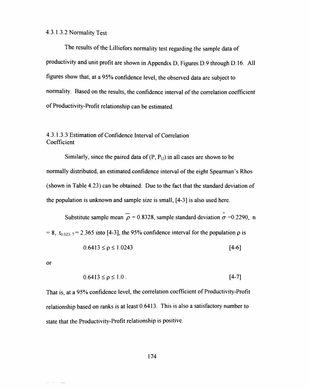
4.3.1.3.2 Normality Test
The resuhs ofthe Lilliefors normality test regarding the sample data of
productivity and unit profit are shown in Appendix D, Figures D.9 through D. 16. All
figures show that, at a 95% confidence level, the observed data are subject to
normality. Based on the results, the confidence interval ofthe correlation coefficient
of Productivity-Profit relationship can be estimated.
4.3.1.3.3 Estimation of Confidence Interval of Correlation Coefficient
Similarly, since the paired data of (P, Pu) in all cases are shown to be
normally distributed, an estimated confidence interval ofthe eight Spearman's Rhos
(shovm in Table 4.23) can be obtained. Due to the fact that the standard deviation of
the population is unknown and sample size is small, [4-3] is also used here.
A
Substitute sample mean p = 0.8328, sample standard deviation a =0.2290, n
^ 8, to 025,7 = 2.365 into [4-3], the 95% confidence interval for the population p is
0.6413 < p < 1.0243 [4-6]
or
0.6413 < p < l . O . [4-7]
That is, at a 95% confidence level, the correlation coefficient of Productivity-Profit
relationship based on ranks is at least 0.6413. This is also a satisfactory number to
state that the Productivity-Profit relationship is positive.
174
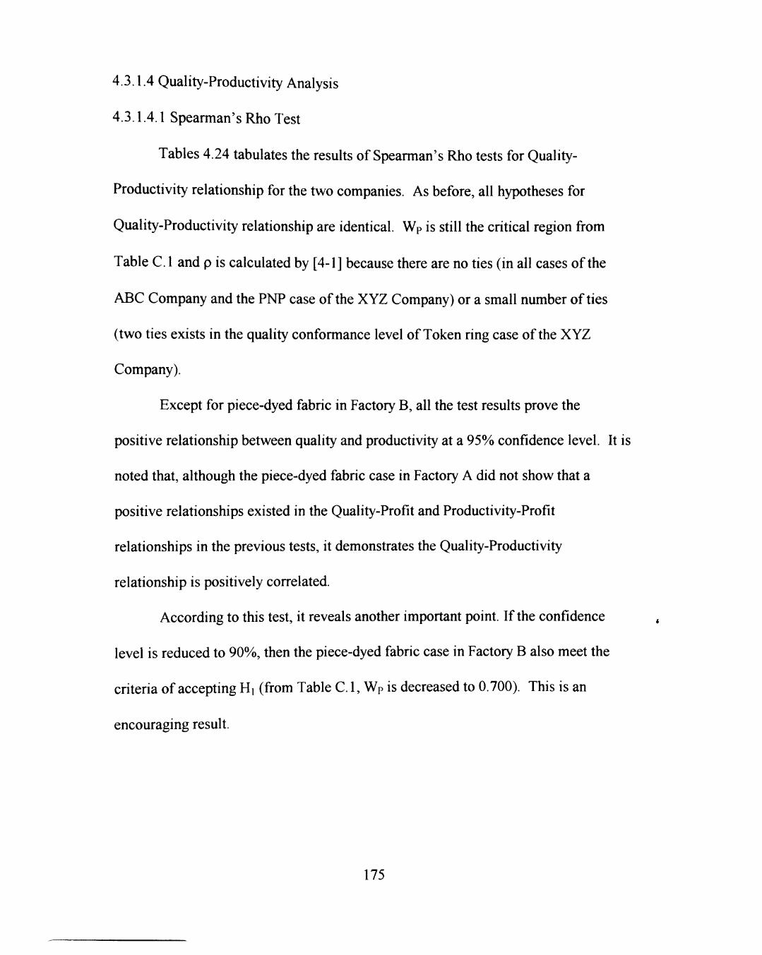
4.3.1.4 Quality-Productivity Analysis
4.3.1.4.1 Spearman's Rho Test
Tables 4.24 tabulates the results of Spearman's Rho tests for Quality-
Productivity relationship for the two companies. As before, all hypotheses for
Quality-Productivity relationship are identical. Wp is still the critical region from
Table C. 1 and p is calculated by [4-1] because there are no ties (in all cases ofthe
ABC Company and the PNP case ofthe XYZ Company) or a small number of ties
(two ties exists in the quality conformance level of Token ring case ofthe XYZ
Company).
Except for piece-dyed fabric in Factory B, all the test results prove the
positive relationship between quality and productivity at a 95% confidence level. It is
noted that, although the piece-dyed fabric case in Factory A did not show that a
positive relationships existed in the Quality-Profit and Productivity-Profit
relationships in the previous tests, it demonstrates the Quality-Productivity
relationship is positively correlated.
According to this test, it reveals another important point. If the confidence
level is reduced to 90%, then the piece-dyed fabric case in Factory B also meet the
criteria of accepting Hi (from Table C. 1, Wp is decreased to 0.700). This is an
encouraging result.
175
Table 4.24 Summary of Spearman's Rho Test Results for Quality-Productivity Relationship
Ho : The quality conformance level and unit productivity are mutually independent
Hi: There is a tendency for the larger values of quality conformance level and productivity to
be paired together
Significance level: a = 0.05
Company
ABC
XYZ
Product
Gingham
Piece-dyed fabric
PNP
Token Ring
Factory A
Critical region: Wp = 0.800
Computed Rho: p =0.800
Conclusion: Accept Hi
Critical region: Wp = 0.800
Computed Rho: p = 0.900
Conclusion: Accept Hi
Factory B
Critical region: Wp = 0.800
Computed Rho: p=1.00
Conclusion: Accept Hi
Critical region: Wp = 0.800
Computed Rho: p = 0.700
Conclusion: Accept Ho
Factory C
Critical region: Wp = 0.800
Computed Rho: p =0.800
Conclusion: Accept Hi
Critical region: Wp = 0.800
Computed Rho: p = 0.900
Conclusion: Accept Hi
Critical region: Wp = 0.3113 Computed Rho: p = 0.9567 Conclusion: Accept Hi Critical region: Wp = 0.3236 Computed Rho: p = 0.9792 Conclusion: Accept Hi
4.3.1.4.2 Normality Test
The results ofthe Lilliefors normality test for the sample data of quality and
productivity are shown in the Appendix D, Figures D. 17 through D.24. All figures
show that, at a 95% confidence level, the observed data are subject to normality.
Based on the results, the confidence interval of correlation coefficient of Quality-
Productivity relationship can be estimated.
176
4.3.1.4.3 Estimation of Confidence Interval of Correlation Coefficient
Based on the results ofthe normality test and the eight Spearman s Rho
(shown in Table 4.24), the confidence interval of correlation coefficient ofthe ranked
Quality-Productivity relationship is estimated by [4-3].
At a 95% confidence level and sample mean p = 0.8796, sample standard
A
deviation a = 0.1044, n = 8, to 025,7= 2.365 yield the following interval
0.7923 < p < 0.9668 . [4-8]
That is, at a 95% confidence level, the correlation coefficient ofthe ranked Quality-
Productivity relationship is at least 0.7923. This number also shows that there is a
highly positively correlated relationship between quality and profit.
According to the hypotheses test and confidence interval estimation,
presented in this subsection, an encouraging result indicates the belief, that the
Quality-Profit, Productivity-Profit, and Quality-Productivity relationships are
positive, is correct. Although this results cannot reveal that how much profit could be
gained by enhancing quality or productivity, it at least indicates that the higher the
quality conformance level or productivity, a larger profit margin is possible.
The more definite relationships of Quality-Profit, Productivity-Profit, and
Quality-Productivity ofthe ABC and XYZ companies are examined in the next
subsection 4.3.2. Specific models were established so that the value of a dependent
variable could be predicted based on a given independent variable.
177
4.3.2 Model Analysis
This section presents the analysis ofthe three models proposed in section
3.2.9. Although the Spearman's Rho tests have shown that the relationships of
Quality-Profit, Productivity-Profit, and Quality-Productivity are positively correlated,
the correlation coefficients could not indicate how they correlated. It is of interest to
know the functions ofthe three relationships. This section looks at the relationships
of Quality-Profit, Productivity-Profit, and Quality-Productivity more precisely. This
section also discusses the aptness ofthe three models. It is obvious that these models
are only applied to the products, factories, and companies being studied.
4.3.2.1 Method of Analysis
Linear regression method based on ranks is used to examine the relationships
of Quality-Profit, Productivity-Profit, and Quality-Productivity. Since the correlation
ofthe relationships, Quality-Profit and Quality-Productivity, were calculated based
on ranks in the previous section and the number of observations in each case are not
large, linear regression based on ranks is applied. As to the Productivity-Profit
relationship, unit profit is directly related to productivity according to the definition
ofproductivity of this research. Therefore, it is not necessary to analyze the
relationship between productivity and unit profit based on sample data.
The linear regression method based on rank is nonparametric. This method
has two basic assumptions: (1) the sample is a random sample, (2) the regression
178
relationship is linear. Data of this research came from the production process and has
been shown to be normally distributed in the preceding subsections 4.3.1.2 through
4.3.1.4, thus the first assumption is met. As to the second assumption, Conover
(1980) indicated that if the relationship between two variables are monotonic, either
increasing or decreasing, their ranks must have a linear relationship. The results of
hypotheses tests presented in subsection 4.3.1 have shown that the ranks of quality,
unit profit, and productivity go hand-in hand. That is, the second assumption is also
met. Therefore, linear regression models can be established and analyzed based on
the ranks of variables.
The procedure for sections 4.2.2.2 through 4.3.2.4 is as follows.
1. Identify the estimated linear regression model based on ranks.
This step is to estimate the linear regression function for each case.
If the estimated model is ofthe form
r( Y) = a + b r(X) [4-9]
where r(X) and r(Y) represent the ranks of variables X and Y,
respectively. Constant a is the intercept ofthe line while b is the
slope. Both a and b are unknovm and must be estimated from the data.
2. Study the residual plot, residual time plot, and residual normality plots to
check the aptness of these specific models.
The aptness of a liner regression model can be examined by four
properties: linearity of regression fimction, constant variance of error
179
terms, independence of error terms, and normality of error terms.^
Linearity and constant variance can be inspected from a residual plot.
The residual time plot diagnoses the independence of error terms. The
residual normality plot inspects the normality of error terms.
4.3.2.2 Quality-Profit Relationship Model Analysis
This subsection first presents the specific Quality-Profit relationship models
for all cases of this research. These models are then examined by residual plots to
inspect their aptness. The plots used here to check the four properties of a linear
regression model contains plots of residuals against the ranks of quality, residuals
against time, and residuals against expected values.
4.3.2.2.1 Specific Linear Regression Models.
The estimated linear regression models ofthe Quality-Profit relationship for
the cases of this research are established and summarized in Table 4.25. Note an
important fact, except for a tiny difference in the Token ring case, the slope of each
^ Error term and residual are different concepts in linear regression analysis. Error term, e, is the vertical deviation of Y from the unknown true regression line and hence is unknown. That is, 8 = Y -E{ Y}. Residual, e, is the vertical deviation from the fitted value on the estimated regression line, and it
A
is known. That is, e = Y - Y
180
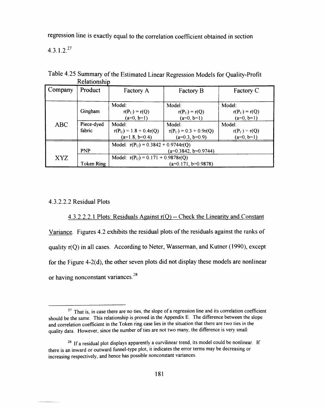
regression line is exactly equal to the correlation coefficient obtained in section
4.3.1.2 27
Table 4.25 Summary ofthe Estimated Linear Regression Models for Quality-Profit Relationship
Company
ABC
XYZ
Product
Gingham
Piece-dyed fabric
PNP
Token Ring
Factory A
Model: r(Pu) = r(Q) (a=0,b=l)
Model: r(Pu)=1.8 + 0.4r(Q)
(a=1.8, b=0.4)
Factory B
Model: r(Pu) = r(Q) (a=0,b=l)
Model: r(Pu) = 0.3 + 0.9r(Q)
(a=0.3, b=0.9)
Factory C
Model: r(Pu) = r(Q) (a=0,b=l)
Model: r(Pr) = r(Q) (a=0,b=l)
Model: r(Pu) = 0.3842 + 0.9744r(Q) (a=0.3842, b=0.9744)
Model: r(Pu) = 0.171 + 0.9878r(Q) (a=0.171,b=0.9878)
4.3.2.2.2 Residual Plots
4.3.2.2.2.1 Plots: Residuals Against r(Q) - Check the Linearity and Constant
Variance. Figures 4.2 exhibits the residual plots ofthe residuals against the ranks of
quality r(Q) in all cases. According to Neter, Wasserman, and Kutner (1990), except
for the Figure 4-2(d), the other seven plots did not display these models are nonlinear
or having nonconstant variances 28
^ That is, in case there are no ties, the slope of a regression line and its correlation coefficient should be the same. This relationship is proved in the Appendix E. The difference between the slope and correlation coefficient in the Token ring case lies in the situation that there are two ties in the quality data. However, since the number of ties are not two many, the difference is very small.
^ If a residual plot displays apparently a curvilinear trend, its model could be nonlinear. If there is an inward or outward funnel-type plot, it indicates the error terms may be decreasing or increasing respectively, and hence has possible nonconstant variances.
181
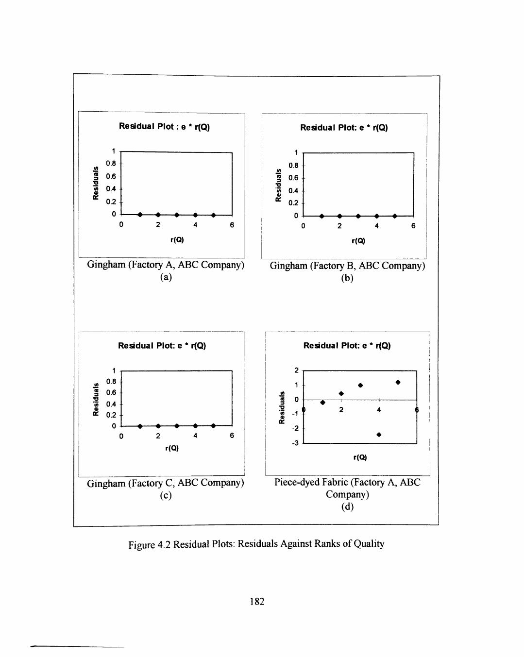
Residual Plot: e * r(Q)
1
0.8
1 0.6 + I 0.4 " 0.2 1
6
r(Q)
Gingham (Factory A, ABC Company) (a)
Residua I Plot: e * r(Q)
j2 ra a •o 'M 0)
OC
1
0.8
0.6 +
0.4
0.2 +
0 6
r(Q)
Gingham (Factory B, ABC Company) (b)
Residual Plot: e * r(Q)
1 « 0.8 1 g 0.6
M 0.4
Oi 0.2
r(Q)
Gingham (Factory C, ABC Company) (c)
Res
idu
als
Residual Plot: e * r(Q)
•7
1
0
-1
-2
-"^ -
• • •
1 2 4 (
•
r(Q)
i
Piece-dyed Fabric (Factory A, ABC Company)
(d)
Figure 4.2 Residual Plots: Residuals Against Ranks of Quality
182
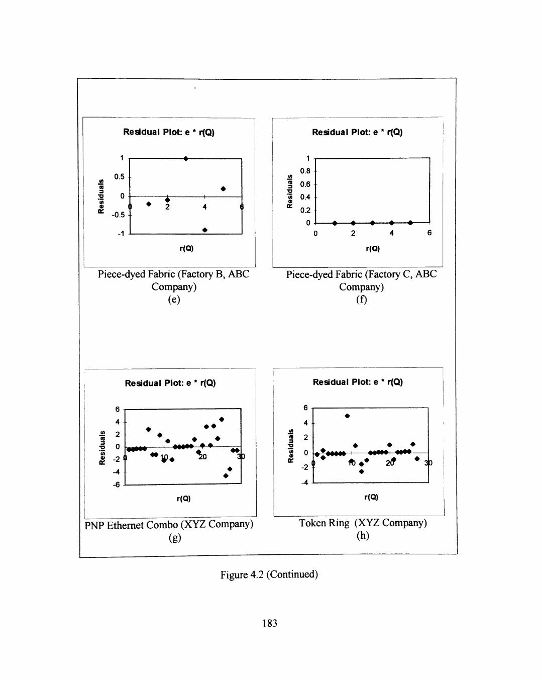
Residual Plot: e * r(Q)
22 ra 3
"35 OC
0.5
-0.5
-1
r(Q)
Piece-dyed Fabric (Factory B, ABC Company)
(e) ua
ls
Res
id
F
1 1
0.8
0.6
0.4
0.2 n
(esidual Plot: e * r(Q)
0 2 4 6
r(Q)
Piece-dyed Fabric (Factory C, ABC Company)
(f)
Res
idu
als
6 1
4
2
0
- 2 '
-4
-6
Residual Plot: e * r(Q)
• • •
1 mmmt% i^ ^
\ **l^# ^0
r(Q)
D
PNP Ethernet Combo (XYZ Company) (g)
Residual Plot: e * r(Q)
4 +
g 2 + "O
35 0
-2 "f
-4
1 ^ * * 2<f 3D
r(Q)
Token Ring (XYZ Company) (h)
Figure 4.2 (Continued)
183
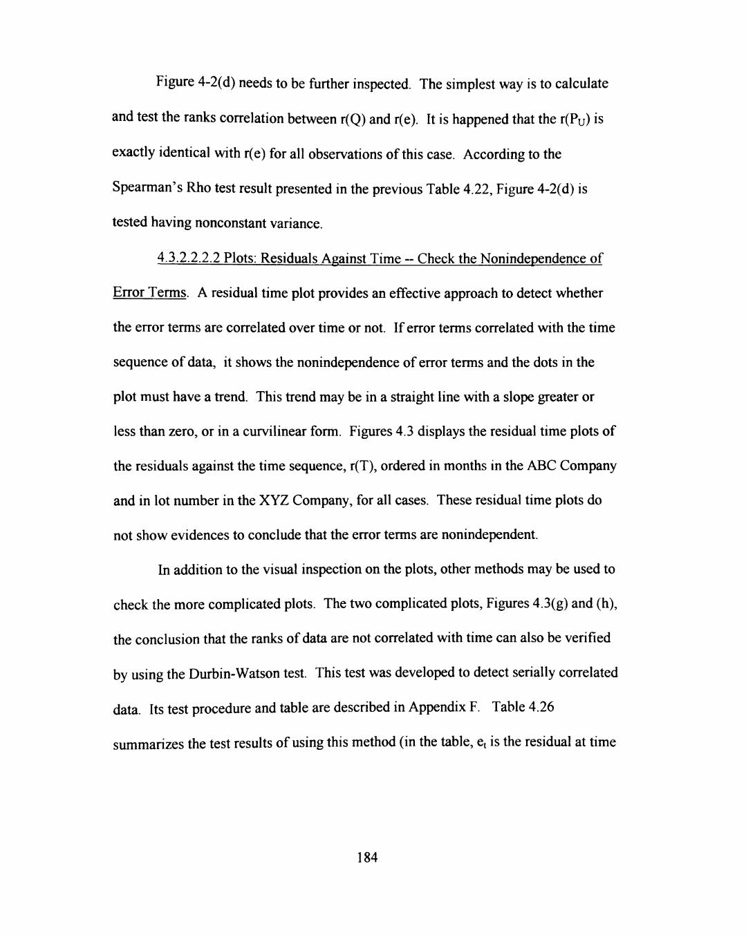
Figure 4-2(d) needs to be further inspected. The simplest way is to calculate
and test the ranks correlation between r(Q) and r(e). It is happened that the r(Pu) is
exactly identical with r(e) for all observations of this case. According to the
Spearman's Rho test result presented in the previous Table 4.22, Figure 4-2(d) is
tested having nonconstant variance.
4.3.2.2.2.2 Plots: Residuals Against Time - Check the Nonindependence of
Error Terms. A residual time plot provides an effective approach to detect whether
the error terms are correlated over time or not. If error terms correlated with the time
sequence of data, it shows the nonindependence of error terms and the dots in the
plot must have a trend. This trend may be in a straight line with a slope greater or
less than zero, or in a curvilinear form. Figures 4.3 displays the residual time plots of
the residuals against the time sequence, r(T), ordered in months in the ABC Company
and in lot number in the XYZ Company, for all cases. These residual time plots do
not show evidences to conclude that the error terms are nonindependent.
In addition to the visual inspection on the plots, other methods may be used to
check the more complicated plots. The two complicated plots. Figures 4.3(g) and (h),
the conclusion that the ranks of data are not correlated yvith time can also be verified
by using the Durbin-Watson test. This test was developed to detect serially correlated
data. Its test procedure and table are described in Appendix F. Table 4.26
summarizes the test results of using this method (in the table, Ct is the residual at time
184
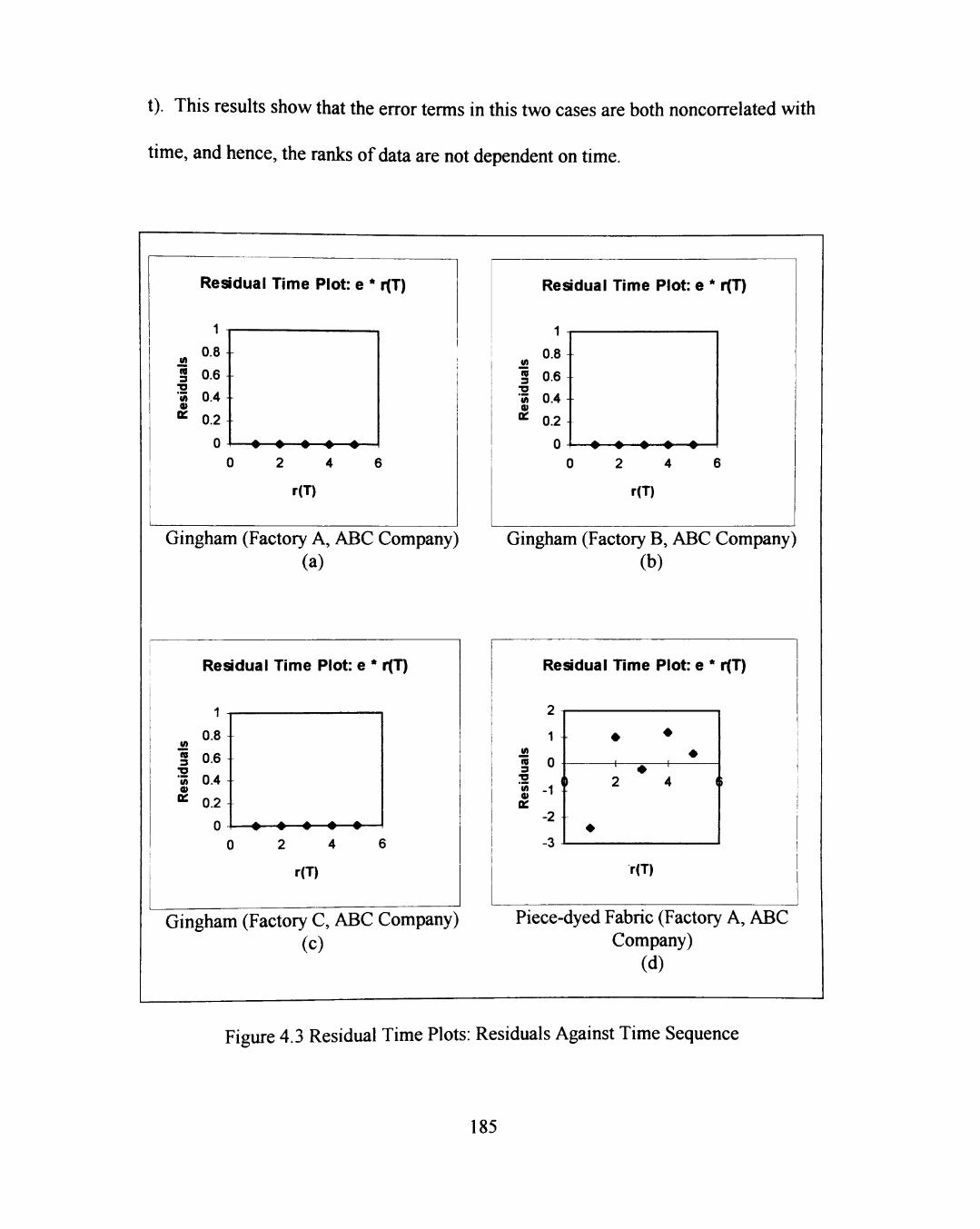
t). This results show that the error terms in this two cases are both noncorrelated with
time, and hence, the ranks of data are not dependent on time.
Residual Time Plot: e * r(T)
M
n 3
Res
id
0.8
0.6
0.4
0.2
0 2 4
r(T)
6
Gingham (Factory A, ABC Company) (a)
Residual Time Plot: e *
1
0.8
§ 0.6 •o
'35 0.4 « • 0.2
n -
r(T)
0 2 4 6
r(T)
Gingham (Factory B, ABC Company) (b)
uals
R
esid
Residual Time Plot: e *
i
0.8
0.6
0.4
0.2 n
0 2 4 e
r(T)
r(T)
Gingham (Factory C, ABC Company) (c)
Residual Time Plot: e * r(T)
1 + re 0
• o •Jfl - 1 :
oc -2 I -3
•
—H
2 4
r<T)
Piece-dyed Fabric (Factory A, ABC Company)
(d)
Figure 4.3 Residual Time Plots: Residuals Against Time Sequence
185
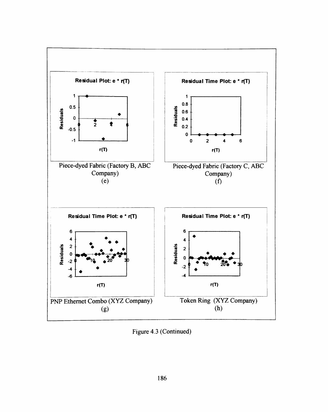
Res
idua
ls
Residual Plot: e * r(T)
1 -•
0.5
0 (
-0.5
-1
•
1 2 t (
•
r(T)
Piece-dyed Fabric (Factory B, ABC Company)
(e)
Residual Time Plot: e *
*
uals
o
o
b>
bo
-
•a •35 0.4 4) ^ 0.2
n -
r(T)
0 2 4 6
r(T)
Piece-dyed Fabric (Factory C, ABC Company)
(f)
Residual Time Plot: e " r(T)
22 ra 3
'55 OC
6
4
2 1-0
-2^
-4
-6
• • •
20 oD
r(T)
PNP Ethernet Combo (XYZ Company) (g)
Residual Time Plot: e * r(T)
R
4
§ 2 •a % 0 a:
-2 _A
•
^ • ^ _ • •
) * to 2dV •s 0
r(T)
Token Ring (XYZ Company) (h)
Figure 4.3 (Continued)
186
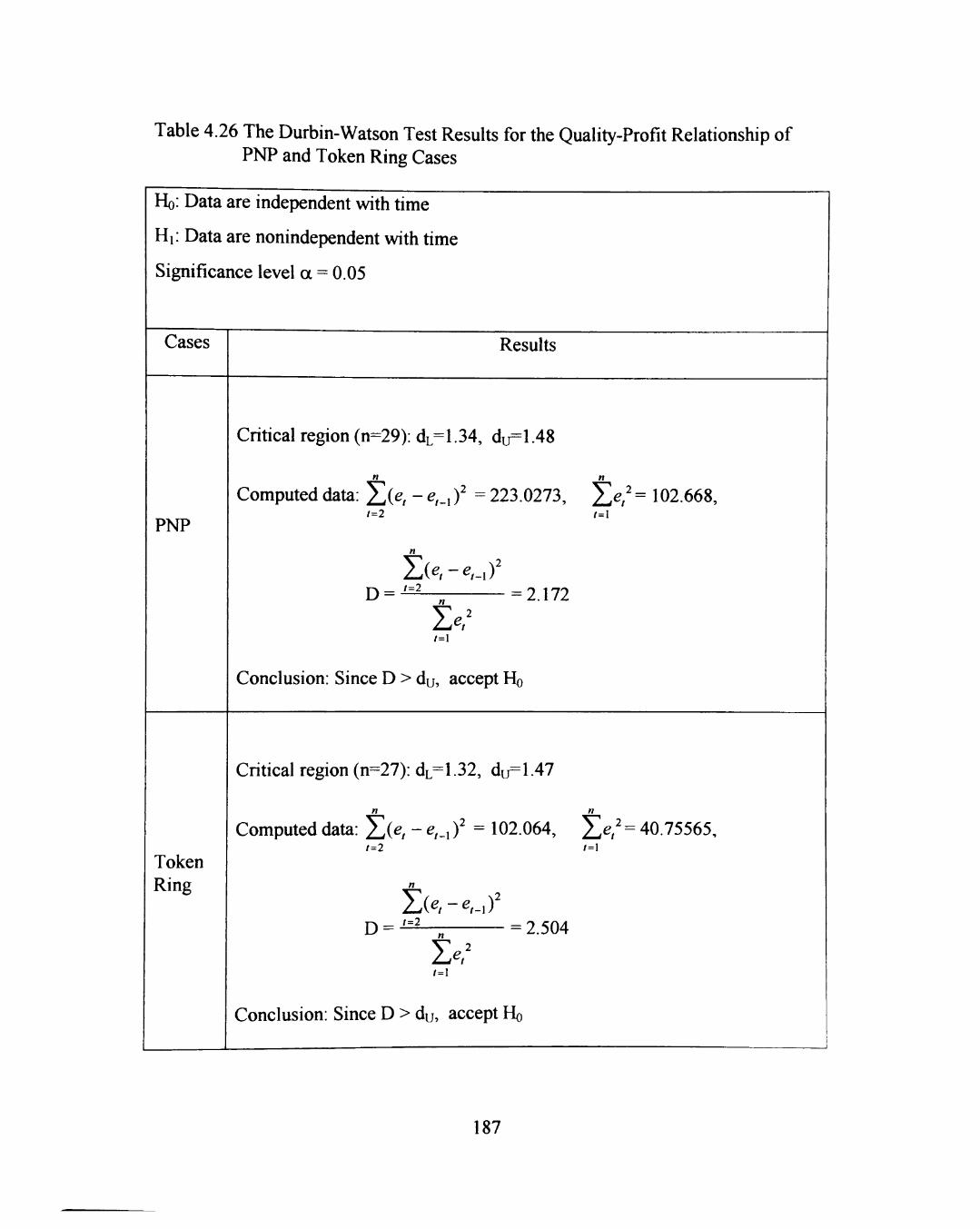
Table 4.26 The Durbin-Watson Test Results for the Quality-Profit Relationship of PNP and Token Ring Cases
HQ: Data are independent with time
Hi: Data are nonindependent with time
Significance level a = 0.05
Cases
PNP
Token Ring
Results
Critical region (n=29): dL=1.34, du=1.48
Computed data: X(^/ " ^t-xf ^ 223.0273, S^/^= 102.668, /=2 t=\
Z(^,-^,-,)' D = - ^ —; = 2.172
Conclusion: Since D > dy, accept Ho
Critical region (n=27): dL=1.32, du=1.47
w n
Computed data: X(^/ " ^/-i)' = 102.064, X^/ ' = 40.75565, 1=2 /=1
D = ^^^ = 2.504
t=\
Conclusion: Since D > du, accept Ho
187
4.3.2.2.2.3 Plots: Residuals Against Expected Values - Check the Normaliy
of Error Terms. This plot is called the normal probability plot ofthe residuals. In
this plot, each residual is plotted against its expected value. If a residuals plot
displays neariy linear form, it suggests agreement with normality. Otherwise, a plot
that departs significantly from linearity reveals that the errors is not subject to a
normal distribution.
According to Neter, Wasserman, and Kutner (1990), statistical theory has
proved that, in a random sample of n, a good approximation ofthe expected value,
EXP VALUE, ofthe ith smallest observation is given by
EXPVALUE = V M S E [ Z ( ^ ~ ' )] [4-10]
where V M S E , mean square error, is the estimated standard deviation which equals
2 i-0.375 (Ee )/(n-2) and z( TT^) is the percentile ofthe standard normal distribution.
This approximation is based on the facts that if the expected values ofthe ordered
residuals is under normality, they must meet two conditions. First, the expected value
ofthe error terms should be zero and second, the standard deviation ofthe error terms
is estimated by V M S E .
Figure 4-4 exhibits the normal probability plots of residuals ofthe specific
models.^^ The ordinate represents the ascending ordered residuals and the abscissa
stands for the residuals' correspondent expected values, obtained by [4-10].
^' There are four cases in which both the residuals and MSE are zeros. They are: Gingham in the Factory A, B, C, respectively, and Piece-dyed fabric in the Factory C. It is apparent that their error
188
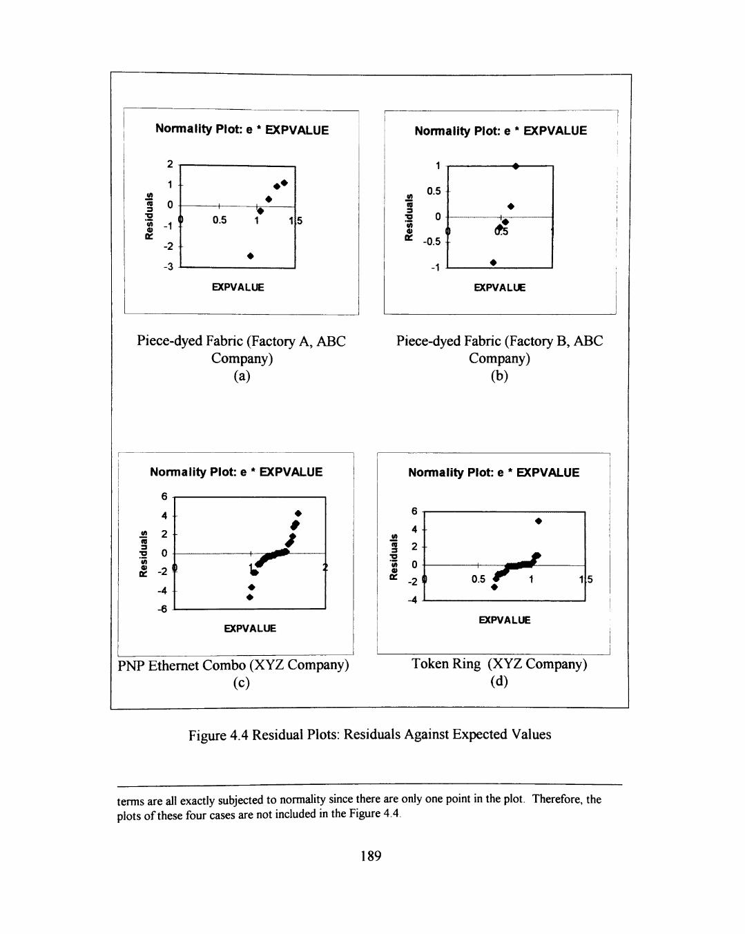
Normality Plot: e * EXPVALUE
2
1
ra 0 j2 "ra 3
tc -2
-3
0.5
EXPVALUE
Piece-dyed Fabric (Factory A, ABC Company)
(a)
Normality Plot: e * EXPVALUE
ra 3
•a '!« OC
0.5
0
-0.5 I
-1
di ;
EXPVALUE
Piece-dyed Fabric (Factory B, ABC Company)
(b)
Normality Plot: e * EXPVALUE
ft
4
« 2 ra
5 0-5 -2
-4
-6
•
1 ]f^
EXPVALUE
;
PNP Ethernet Combo (XYZ Company) (c)
No
6
4 -ra p , 3 ^
"35 0 Oi
^ . 2 (
-4 ^
nmality Plot: e * EXPVALUE
•
1 0.5 r ^ 1 1
EXPVALUE
5
Token Ring (XYZ Company) (d)
Figure 4.4 Residual Plots: Residuals Against Expected Values
terms are all exactly subjected to normality since there are only one point in the plot. Therefore, the plots of these four cases are not included in the Figure 4.4.
189
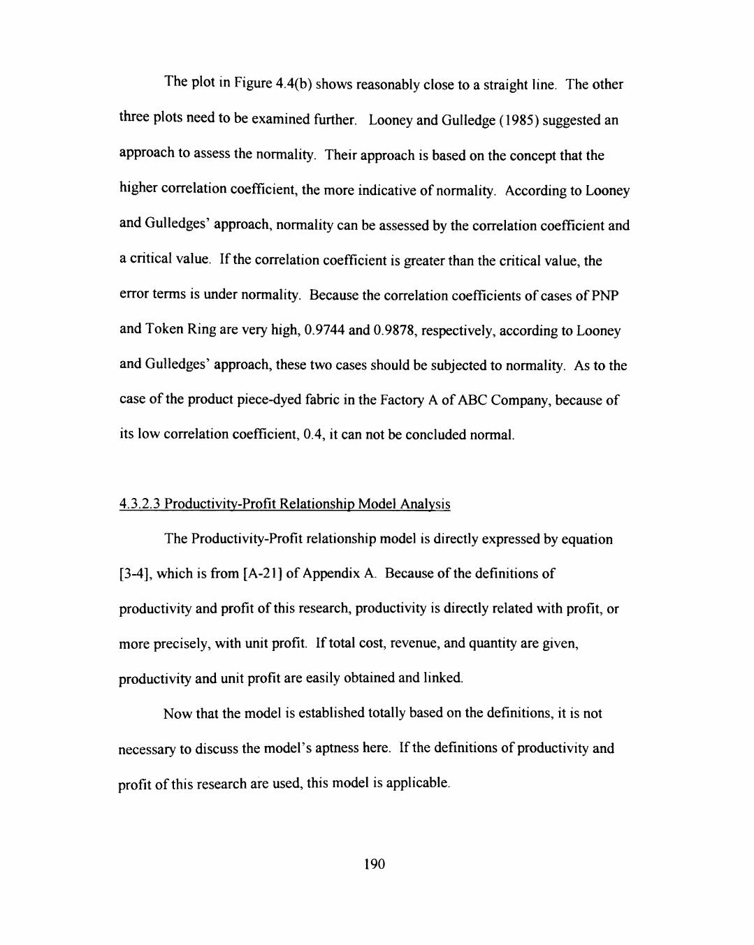
The plot m Figure 4.4(b) shows reasonably close to a straight line. The other
three plots need to be examined further. Looney and Gulledge (1985) suggested an
approach to assess the normality. Their approach is based on the concept that the
higher correlation coefficient, the more indicative of normality. According to Looney
and Gulledges' approach, normality can be assessed by the correlation coefficient and
a critical value. If the correlation coefficient is greater than the critical value, the
error terms is under normality. Because the correlation coefficients of cases of PNP
and Token Ring are very high, 0.9744 and 0.9878, respectively, according to Looney
and Gulledges' approach, these two cases should be subjected to normality. As to the
case ofthe product piece-dyed fabric in the Factory A of ABC Company, because of
its low correlation coefficient, 0.4, it can not be concluded normal.
4.3.2.3 Productivity-Profit Relationship Model Analysis
The Productivity-Profit relationship model is directly expressed by equation
[3-4], which is from [A-21] of Appendix A. Because ofthe definitions of
productivity and profit of this research, productivity is directly related with profit, or
more precisely, with unit profit. If total cost, revenue, and quantity are given,
productivity and unit profit are easily obtained and linked.
Now that the model is established totally based on the definitions, it is not
necessary to discuss the model's aptness here. If the definitions ofproductivity and
profit of this research are used, this model is applicable.
190
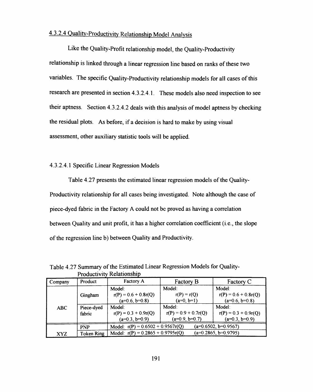
4.3.2.4 Quality-Productivity Relationship Model Analysis
Like the Quality-Profit relationship model, the Quality-Productivity
relationship is linked through a linear regression line based on ranks of these two
variables. The specific Quality-Productivity relationship models for all cases of this
research are presented in section 4.3.2.4.1. These models also need inspection to see
their aptness. Section 4.3.2.4.2 deals with this analysis of model aptness by checking
the residual plots. As before, if a decision is hard to make by using visual
assessment, other auxiliary statistic tools will be applied.
4.3.2.4.1 Specific Linear Regression Models
Table 4.27 presents the estimated linear regression models ofthe Quality-
Productivity relationship for all cases being investigated. Note although the case of
piece-dyed fabric in the Factory A could not be proved as having a correlation
between Quality and unit profit, it has a higher correlation coefficient (i.e., the slope
ofthe regression line b) between Quality and Productivity.
Table 4.27 Summary ofthe Estimated Linear Regression Models for Quality-Productivity Relationship
Company
ABC
XYZ
Product
Gingham
Piece-dyed fabric
PNP Token Ring
Factory A
Model: r(P) = 0.6 + 0.8r(Q)
(a=0.6, b-0.8) Model:
r(P) = 0.3 + 0.9r(Q) (a=0.3, b=0.9}
Factory B Model:
r(P) = r(Q) (a=0, b=l)
Model: r(P) = 0.9 + 0.7r(Q)
(a=0.9, b=0.7)
Factory C Model:
r(P) = 0.6 + 0.8r(Q) (a=0.6, b=0.8)
Model: r(P) = 0.3 + 0.9r(Q)
(a=0.3, b=0.9)
Model: r(P) = 0.6502 + 0.9567r(Q) (a=0.6502, b=0.9567) Model: r(P) = 0.2865 + 0.9795r(Q) (a=0.2865, b=0.9795)
191
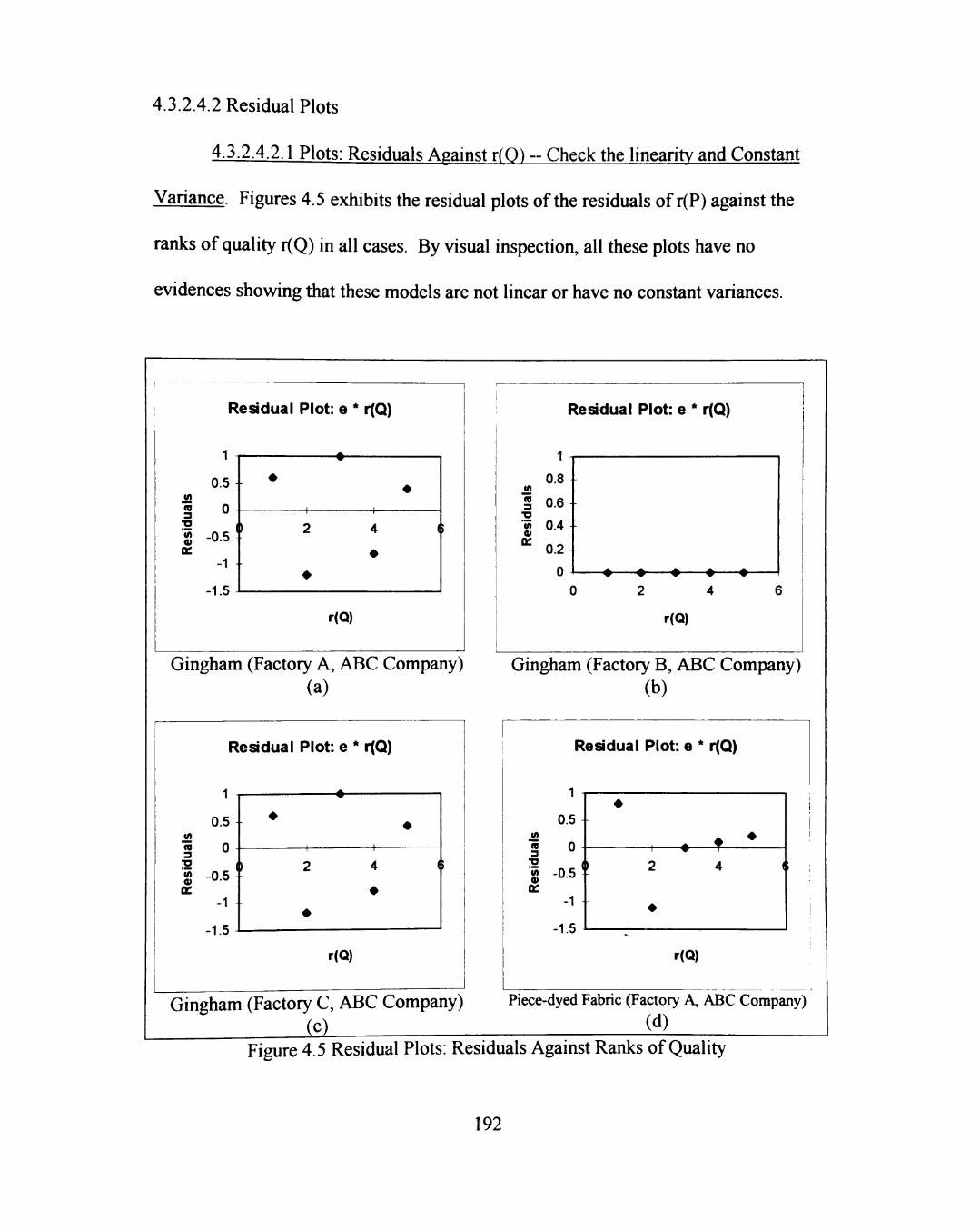
4.3.2.4.2 Residual Plots
4.3.2.4.2.1 Plots: Residuals Against r(0) - Check the linearity and Constant
Variance. Figures 4.5 exhibits the residual plots ofthe residuals of r(P) against the
ranks of quality r(Q) in all cases. By visual inspection, all these plots have no
evidences showing that these models are not linear or have no constant variances.
Restdual Plot: e * r(Q)
0.5 +
CO 0
S -0.5 1 OC
-1 + -1.5
4
r(Q)
Gingham (Factory A, ABC Company) (a)
Residual Plot: e * r(Q)
1
0.5
ra 0 3 •g -0.5 1 OC
-1
-1.5
4
•
r(Q)
Residual Plot: e * r(Q)
0.8
5 0.6 •o w 0.4 » • 0.2
n
( ) 2 4 6
r(Q)
Gingham (Factory B, ABC Company) (b)
Residual Plot: e * r(Q)
1
0.5
0 -J2 ra 3 "O •« -0 5 -OC
-1 +
-1.5
r(Q)
Gingham (Factory C, ABC Company) Piece-dyed Fabric (Factory A, ABC Company) (c) (d)
Figure 4.5 Residual Plots: Residuals Against Ranks of Quality
192
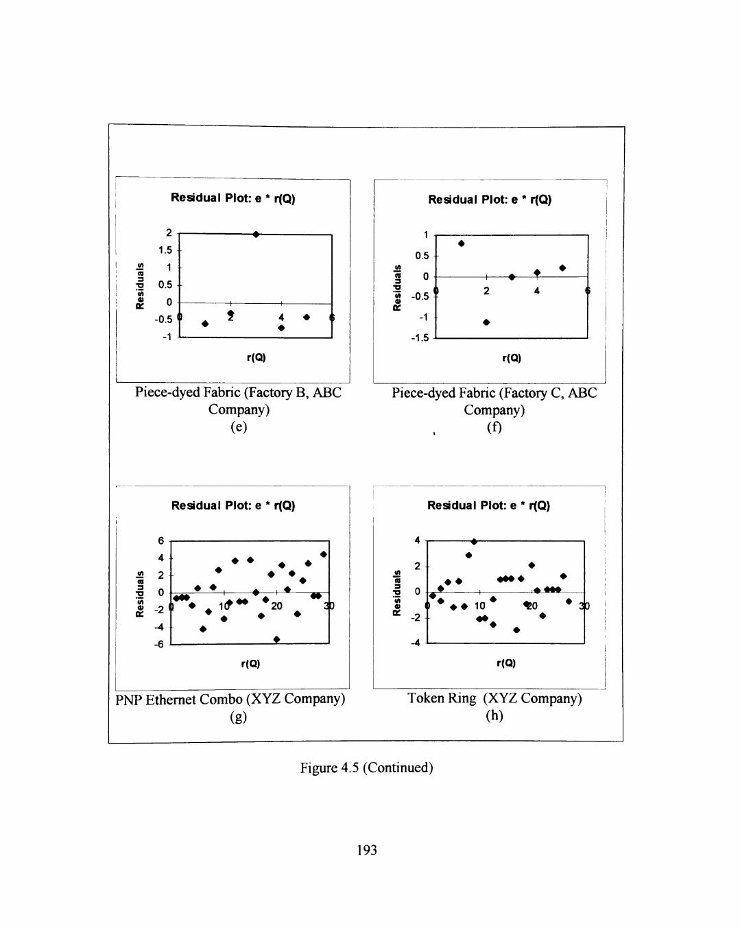
Residual Plot: e * r(Q)
_j2 ra 3
•o 'vi «
OC
1.5
1
0.5
0 -
-0.5 i'
-1 -
—1
4 •
r(Q)
Piece-dyed Fabric (Factory B, ABC Company)
(e)
Residual Plot: e * r(Q)
1
0.5
1 0
"5! -0 5 T OC
-1 + -1.5
\
r(Q)
Piece-dyed Fabric (Factory C, ABC Company)
(0
Residual Plot: e * r(Q)
6
4 jrt 2 ra
^ -2? -4
-6
• •
• •
• •
^ ^ ^ I ^ — ^ ^
i(f 20 CD
r(Q)
PNP Ethernet Combo (XYZ Company) (g)
Residual Plot: e * r(Q)
2 + "5 I 0 «A «
" -2 +
-4
• •
• • • 1 0 * « 0 3D
r(Q)
Token Ring (XYZ Company) (h)
Figure 4.5 (Continued)
193

4.3.2.4.2.2 Plots: Residuals Against Time - Check the Nonindependence of
Error Terms. Figures 4.6 displays the residual time plots ofthe residuals of r(P)
against the time sequence, r(T) for all cases. These residual time plots fail to show
evidences to conclude that the error terms are nonindependent.
Residual Time Plot: e *
1 -^
0.5 (A
ra 0
2 -0.5' OC
-1
-1.5
1 2 4 (
r(T)
r(T)
1
Gingham (Factory A, ABC Company) (a)
Residual Time Plot: e *
1
0.8
S 0.6 •o
•«» 0.4 « • 0.2
n -
r(T)
0 2 4 6
r(T)
Gingham (Factory B, ABC Company) (b)
Residual Time Plot: e * r(T)
0.5 vt ra 0
2 - 0 . 5 ; oc
-1
-1.5
4
•
r(T)
Gingham (Factory C, ABC Company) (c)
Residual Time Plot: e * r(T)
1
0.5
ra 0 2 ( « -0.5 ' « OC
-1 1 c
•
• • T 1 2 4 1
•
i
r(T)
Piece-dyed Fabric (Factory A, ABC Company)
(d)
Figure 4.6 Residual Time Plots: Residuals Against Time Sequence
194
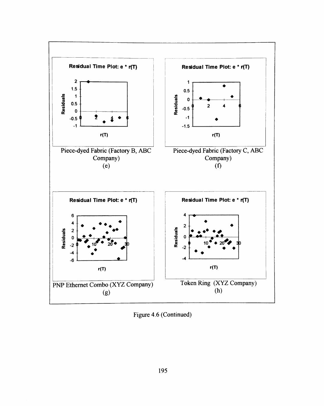
Residual Time Plot: e * r(T)
J2 ra 3
"35 «
OC
2
1.5
1
0.5
0
-0.5
-1 • i * i;
r(T)
Piece-dyed Fabric (Factory B, ABC Company)
(e)
Residual Time Plot: e * r(T)
0.5 J2 ra
2 -0.5 OC
-1
-1.5
r(T)
Piece-dyed Fabric (Factory C, ABC Company)
(f)
Residual Time Plot: e * r(T)
V) ra
6
4
2
0 2
^ -2l|l
-4
-6
• •
• • •» # : >
10 2 0 * 30
r(T)
PNP Ethernet Combo (XYZ Company) (g)
Residual Time Plot: e * r{T)
ra 3
« 0
4
2
0
-2
• » I ^ • t
1 0 * • 2 0 ^ 3P • • •
r(T)
Token Ring (XYZ Company) (h)
Figure 4.6 (Continued)
195

Further confirmation by using the Durbin-Watson test are needed for the two
complicated plots. Figures 4.6(g) and (h). Table 4.28 summarizes the test results by
using this method. The results indicate that the error terms in these two cases are
both noncorrelated with time. That means the ranks of data are independent of time.
Table 4.28 The Durbin-Watson Test Results for the Quality-Productivity Relationship of PNP and Token Ring Cases
HQ: Data are independent wdth time
Hi: Data are nonindependent with time
Significance level a = 0.05
Cases Results
PNP
Token
Ring
Critical region (n=29): dL=1.34, du=1.48 n n
Computed data: Z(^, "^/-i)' =490.7562, X ^ / = 172.1852, t=2
D =
/=i
lL(e,-e,J t=2
n 2.850
Conclusion: Since D > du, accept Ho
Critical region (n=27): dL=1.32, du=1.47
Computed data: Y.{e, - e,_, f = 144.0387, X^,' = 67.31445, /=2
D =
/=i
Y.(e,-e,J t=2
t=\
= 2.140
Conclusion: Since D > du, accept HQ
196
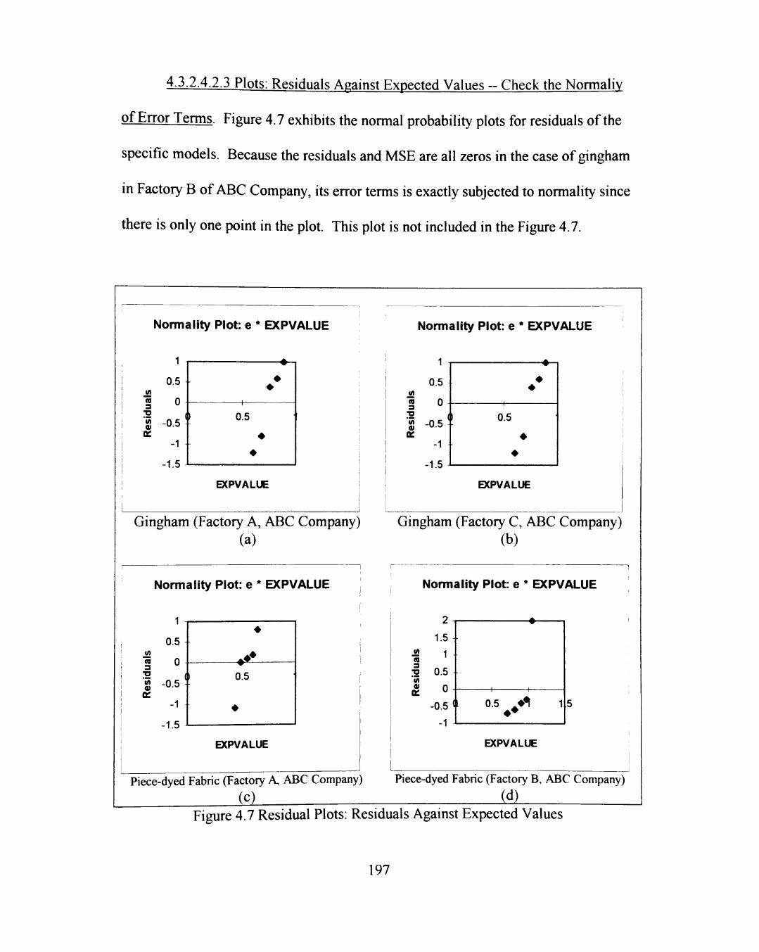
4.3.2.4.2.3 Plots: Residuals Against Expected Values - Check the Normaliy
of Error Terms. Figure 4.7 exhibits the normal probability plots for residuals ofthe
specific models. Because the residuals and MSE are all zeros in the case of gingham
in Factory B of ABC Company, its error terms is exactly subjected to normality since
there is only one point in the plot. This plot is not included in the Figure 4.7.
Normality Plot: e * EXPVALUE Normality Plot: e * EXPVALUE
M ra 3 "O
Q£
1
0.5
0 1
« ^ ( -U.b
-1
- 1 . 5 J
1 0.5
•
•
EXPVALUE
(A ra 3 12 tn 0) OC
0.5
n ^ ^ (
-O.b
-1
- 1 «; -
,
0.5
•
•
EXPVALUE
Gingham (Factory A, ABC Company) Gingham (Factory C, ABC Company) (a) (b)
Normality Plot: e * EXPVALUE Normality Plot: e * EXPVALUE
1
0.5 +
0 jn ra 3
•g -0.5
-1 +
-1.5
0.5
EXPVALUE
ra
3
0)
OC
1.5 1
0.5
0 -
-0.5 <»
-1 -
0.5 ^4^
EXPVALUE
Piece-dyed Fabric (Factory A, ABC Company) Piece-dyed Fabric (Factory B, ABC Company)
(Cl (d) Figure 4.7 Residual Plots: Residuals Against Expected Values
197
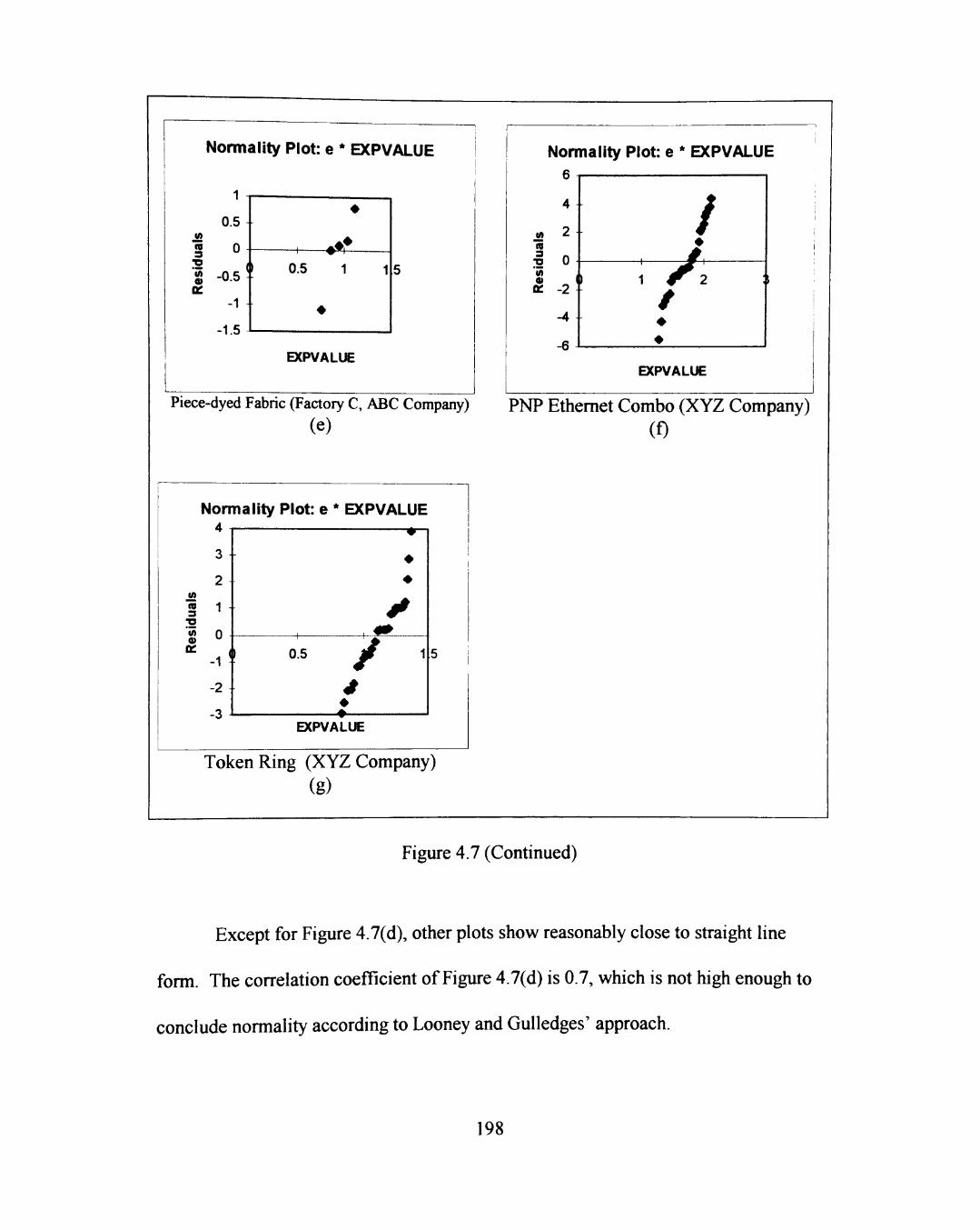
Normality Plot: e * EXPVALUE
1
0.5 +
0 J2 ra 3 "D S -0.5 T oc
-1 + -1.5
.•e 0.5 1
EXPVALUE
Piece-dyed Fabric (Factory C, ABC Company)
(e)
Normality Plot: e * EXPVALUE 6
4
tn 2 ra
I 0 oc -2\
-4
-6
/
/ ^
•
•
EXPVALUE
PNP Ethernet Combo (XYZ Company) (f)
Normality Plot: e * EXPVALUE A ,
3
2 M
•o
t 0
-2
-3
•
• •
• 1 0.5 j r 1
EXPVALUE
5
Token Ring (XYZ Company) (g)
Figure 4.7 (Continued)
Except for Figure 4.7(d), other plots show reasonably close to straight line
form. The correlation coefficient of Figure 4.7(d) is 0.7, yvhich is not high enough to
conclude normality according to Looney and Gulledges' approach.
198
4.4 General Discussion
This section presents a discussion on the results of data analysis of section
4.3. This discussion includes the summarized statement, confidence level, and the
specific models of Quality-Profit and Quality-Productivity relationships.
Productivity-Profit relationship is discussed from the theoretical viewpoint. In
addition, several points regarding the data collected are also discussed.
4.4.1 Discussion of Quality-Profit Relationship
According to the results of hypotheses tests listed in Table 4.22, it is
acceptable to claim that product quality positively affects unit profit. Among the
eight cases, seven cases confirmed that the ranks of quality and unit profit have a
positive relationship through the hypotheses test. Only one case, piece-dyed fabric in
Factory A of ABC Company, failed to confirm this positive relationship. However, in
this case, it does not mean that this relationship is negative or irrelevant. From the
statistical viewpoint, when a hypothesis test fails to reject the null hypothesis, it
simply means there is not sufficient evidence based on sample data to accept the
alternative hypothesis. In fact, the correlation coefficient of this failed case is 0.4,
which also shows positive relationship between quality and unit profit; however,
based on sample data, this statement failed to be proved.
The smallest coefficient of correlation of population between the ranks of
quality and unit profit, based on the eight cases, is 0.7339. This number which was
199
calculated based on 95% confidence level came from the interval inference by
equation [4-3]. However, since this coefficient cannot exceed one, the confidence
level can be reduced. In equation [4-5], the required confidence level for the largest
p, 1, is 75%.^^ At this confidence level, the left-hand side p is 0.8154. This number
reveals a high correlation between the ranks of quality and unit profit.
The results ofthe specific models analyzed (section 4.3.2.2) shows that, all
models are applicable except the case of piece-dyed fabric in the Factory A of ABC
Company. The observations and predicted values of unit profit based on the specific
models are tabulated in the Appendix G. Note the predicted unit profits ofthe four
cases, gingham in the three factories and piece-dyed fabric in Factory A, exactly fit
the models. Hence, the predicted value is exactly the same as the observed data.
4.4.2 Discussion of Productivity-Profit Relationship
Theoretically, according to the equation [A-21] of Appendix A, the
productivity is directly related to unit profit. This is because productivity and unit
profit are such defined that they relate with each other. However, there are still two
variables that affect this relationship, i.e., total cost I and production quantity V. One
important assumption ofthe model development of this research is based on "when
quality is enhanced, unit cost, W, decreases or at least does not increase."
" According to equation [4-3], if the right-hand side equals one, taa must be 1.2557. That means the cumulative probability for 1 - a/2 is 0.875.
200
According to [A-21], when quality increases, unit profit increases as productivity
increases.
There are three reasons for the assumption, "the enhancement of quality will
decrease or not increase the unit cost." First, the decreases in defective products or
rework reduces costs and hence, increase revenue. Second, overhead costs are
reduced due to the more stable process. Third, the benefit from larger sales reduces
unit cost. Therefore, nearly all researchers, such as Deming (1986), Juran (1993),
Feigenbaum (1983), Crosby, P. B. (1979), maintain that enhanced quality must
decrease costs. Therefore, the pursuit of higher product quality is encouraged.
The test results ofthe field data listed in Table 4.23 demonstrates the high
correlated relationship between productivity and unit profit. In theory, it should
exactly correlate, but the test ofthe field data does not show this exact relationship.
This is due to the discrepancy between the assumption just mentioned and physical
data. There are two potential causes for this discrepancy: the assumption is fallacious
or the field data collected is incorrect. However, since many researchers assert that
higher quality will reduce cost and this research agrees, the only possible cause is the
field data. Perhaps, this is another topic for the interested researchers to conduct a
long-term confirmatory study to clarify the relationship between quality and
production cost.
201
4.4.3 Discussion of Quality-Productivity Relationship
According to the results of hypotheses tests listed in Table 4.24, it is
acceptable to claim that product quality is positively related to productivity. Among
the eight cases, seven cases confirmed that the ranks of quality and productivity have
a positive relationship through the hypotheses test. Only one case, piece-dyed fabric
in the Factory B of ABC Company, failed to confirm this positive relationship at
confidence level 95%. However, if confidence level is reduced to 90%, the
conclusion ofthe hypothesis test changes to accept the alternative hypothesis. This
result shows that a positive relationship between the ranks of quality and productivity
exists, which also indicates that quality and productivity is positively correlated.
The coefficient of correlation of population between the ranks of quality and
productivity, based on the eight cases, could be higher than 0.7923. This number
shows the ranks of quality and productivity positively correlated with at least 0.7923
coefficient based on 95% confidence level. This number reveals a high correlation
between the ranks of quality and productivity. Therefore, it is satisfactory to claim
that quality and productivity are positively correlated.
The results ofthe specific analyses of models presented in section 4.3.2.4
show that, all models are applicable except the case of piece-dyed fabric in the
Factory B of ABC Company. The observations and predicted values ofproductivity
based on the specific models are tabulated in the Appendix H. The predicted
202
productivity ofthe product gingham in the Factory B, exactly fit the models. Hence,
the predicted value is exactly the same as the observed data.
The case that failed to fit the model, piece-dyed fabric in the Factory B, is due
to the nonnormality of its data. Because the sample size is not large, one outlier may
severely influence the resuh. It is reasonable to suspect the upper point in Figure
4.7(d) might be an outlier; however, without sufficient evidence, no further action
can be done to disregard this point.
4.4.4 Discussion of Data
There are three problems regarding the data of this field research which must
be addressed. These problems influence the results of data analysis.
The first problem lies in the sample size, especially in the ABC Company.
Although in each case ofthe ABC Company there are only five sample data, five of
the six cases confirm the positive relationship. In the two cases of XYZ Company,
both sample sizes are much larger, also verify this relationship. Based on these
results, the confirmation is, in general, satisfactory.
The second problem of this field study is about the quality conformance level.
Three points regarding this problem need to be noted: (1) The data of quality
conformance level is converted from the original data, which is not measured in %;
(2) Different products have different quality criteria; therefore, conformance level has
different meanings for different products; (3) These values of quality data (%) are
203
very close. Due to this fact, using the concept of ranks may be a better way to
compare with productivity or profit.
The third problem regarding the relationships of Quality-Profit, Productivity-
Profit, and Quality-Productivity concerns the data of production quantity. Because
quantity affects cost, revenue, and profit, it must be taken into account when attempt
to relate quality, profit, and productivity. This is the reason that unit profit, instead of
profit, is used through this research.
204
CHAPTER 5
CONCLUSIONS AND RECOMMENDATIONS
This chapter summarizes this research, presents further discussion and
conclusions, and provides recommendations for the future research. The summary,
presented in section 5.1, briefly illustrates the features and contributions of this
research. Section 5.2 gives further discussion and implications which are not
mentioned in the previous chapters. Conclusions are summarized in several points to
highlight the applicability of this research and is addressed in section 5.3. In the last
section, 5.4, recommendations for the future research are proposed from both the
theoretical and practical standpoints.
5.1 Summary
This research investigates the relationships of Quality-Profit, Productivity-
Profit, and Quality-Productivity. The Quality-Productivity relationship is a
controversial topic, especially prevalent in the manufacturing industries. In order to
realize this relationship, it is better to connect them with an intermediate variable.
This research believes the best intermediate variable is profit because it is one of
management's main concerns. Therefore, at first, it is essential to understand the
relationships between quality and profit, and productivity and profit. However,
205
because profit is affected by sales quantity, it is better to choose the unit profit to
compare with other variables.
Most ofthe literature review of this research demonstrates that the Quality-
Productivity relationship should be positive; however, few of them could prove this
assertion. The few who presented their mathematical models had several key
concepts that were not clarified: (1) quality cost was synonymous with production
cost, (2) no mention ofthe influence of sales quantity, (3) quality conformance level
(%) was regarded as an interval or ratio scale of measurement, (4) no explanation of
how quality could be measured to get unit of measure in %.
In order to improve these deficiencies ofthe current models regarding
Quality-Productivity relationship, this research utilizes the concept of ranks to relate
variables based on unit profit. In addition, the cost used in this research is production
cost, not quality cost, which is difficult to accurately measure under the current cost
accounting system used by most industries.
This research investigates the relationships of Quality-Profit, Productivity-
Profit, and Quality-Productivity in two ways: theoretical and practical. The
theoretical models of Quality-Profit, Productivity-Profit, and Quality-Productivity
relationships are summarized in Table 5.1. For detailed development of these models
refer to Appendix A. These models are developed so that they are generic to
manufacturing environments. These three models show that the three relationships
are all positively correlated.
206

Table 5.1 Summary of Mathematical Models of This Research
Relationship
Quality-Profit
Productivity-Profit
Quality-Productivity
Model
r(Pu) = a, + b,r(Q),
Zr(Qi)r(Pui)-n(n+l)V4
bi = - 4 , Z[r (Q.) ] ' -n(n +1)^/4 i = l
ai = (l-b,)(n+l)/2.
Pu = ( P - l ) x ^
r(P) = a2 + b2r(Q)
Zr(Q.)r(P,)-n(n +1)^/4
Z [ r ( Q . t f - n ( n + l ) V 4 i = l
a2 = (l-b2)(n+l)/2.
In the field study part of this research, two companies in Taiwan were
selected to confirm the relationships. The analysis of field data verified the
207
alternative hypotheses that all three relationships are positively related. In addition,
specific models for the investigated cases were also presented in Tables 4.25 and
4.27. By model analysis, most ofthe specific models are suitable to the cases. This
result makes firm the belief that there must be a positive relationship between quality,
unit profit, and productivity.
5.2 Further Discussion and Implications
Section 5.2.1 addresses some issues that need to be further discussed.
Besides, section 5.2.2 presents implications of this research. These implications
extend the explanations for the results of this research.
5.2.1 Further Discussion
There are two key assumptions in the model development of this research in
Appendix A. One assumption is, "all conformed goods could be sold." In the real
world, whether all conformed goods can be sold is questionable. This problem
involves pricing strategy, product innovation, and other factors such as damage
caused by storage, shipping and handling. However, due to the difficulty of
measurement, these factors are not taken into account in the models.
The other assumption, "that unit cost will not increase when quality
improves," was asserted by most researchers. Based on this assertion, quality
improvement is encouraged; otherwise, the question arises as to whether it is
208
profitable to improve product quality. Therefore, this assertion becomes an important
statement of this research.
In addition to the assumptions addressed above, there are two other important
variables that affects the relationships of quality, profit, and productivity, not
addressed in this research. These two influential factors are marketability and
production capacity. Even though the PIMS has proved in practice that better quality
results in bigger market share, and hence, produces more profit, this research handles
this factor as a constant. This means, in fact, the profit that will be created is higher
than the estimated value ofthe proposed model of this research. Therefore, models
of this research are conservative in estimating profits.
Production capacity is also considered satisfactory when relating the variables
of quality, profit and productivity. The better product quality will "pull" more
demand from market, and then "push" the necessity of expanding production.
Therefore, in this research, capacity as assumed can increase with the demand
v^thout difficulty.
5.2.2 Implications
The implications of this research includes the following points:
1. Even though the product quality is not measured in conformance level (e.g.,
measured in defects per one hundred pieces), according to rank, the model
is still appHcable.
209
2. Models that failed to be applied can possibly be remedied by methods, such
as enlargement of sample size, adding weights to data (e.g., different
weights for different lots), transform nonlinear regression into linear, or
examine the questionable data to exclude the outliers, etc. To remedy the
two cases in which models are not apt to use would be meaningless because
the sample size is too small.
3. If the relationship between two variables is categorized into five classes
according to its correlation coefficient:
• Exactly correlated p = I
• Highly correlated 0.67 < p < 0.99
• Mediumly correlated 0.34 < p < 0.66
• Low correlated 0.01 < p < 0.33
• Exactly independent p = 0
then, the relationships of Quality-Profit, Productivity-Profit, and
Quality-Productivity in the investigated companies could be classified as
highly correlated.
4. This research strongly suggests that the relationships of Quality-Profit and
Quality-Productivity from the viewpoint of improving quality is positively
related. That is, if quality is improved, then unit profit and productivity
should increase. However, if the assumption of unit cost changed, from
"not increase" to "not decrease," the results of this research are still
210

applicable. That is, when quality is lowered, the unit profit and
productivity should also decrease.
5.3 Conclusions
Conclusions of this research are summarized in the following points.
1. The proposed mathematical models of this research were validated through
the field study.
2. Although the positive relationships were verified by the ranks, it also
shows that the variables for quality, profit, and productivity are positively
related.
3. The result of this research supports the concept of kaizan (continuous
improvement). That is, the more improvement in quality or productivity,
the more profit will be created.
4. Specific models based on ranks could be established and verified in other
cases where definitions of quality, productivity, and profit may differ from
this research.
5. That quality must be measured in conformance level is not necessary.
When in application, the model only needs the ranks of quality. Therefore,
this model can be applied more yvddely.
211
6. Although the specific models are only suitable to the investigated
companies, the approach to link variables as well as the mathematical
models are believed to be genenc to all industries.
5.4 Recommendations
Recommendations regarding this research are separated into two parts,
theoretical and practical recommendations. These are addressed next respectively.
5.4.1 Theoretical Recommendations
To the researchers who are interested in studying further the relationship
between quality and productivity, this research recommends that the follov^ng issues
be taken into account.
1. Besides the nonparametric statistical approach, there may exist other
approaches to connect the quality, profit, and productivity. However, be
cautious of whether the data are of interval or ratio scales of measurement.
2. Quality, profit, and productivity may be defined in different ways; however,
they must be operationally defined such that the relationships between them
can be clearly understood.
3. Further exploration on the relationship between quality and productivity
based on quality cost may be feasible; however, the relationship between
quality cost and production cost must be first clarified.
212
5.4.2 Practical Recommendations
The purpose of studying the relationships of Quality-Profit, Productivity-
Profit, and Quality-Productivity is to ensure management that the enhancement of
quality and productivity will create higher profit. In order to reach this, the following
steps are suggested:
1. Define clearly the terms used for desired performance measures. Different
definitions may result in totally different performance index.
2. Develop specifically the steps to measure the performance index.
3. Implement strictly according to the steps for measuring the required data.
4. Develop models based on the observed data and predict values for future
control.
5. Examine the models by its assumptions.
6. Amend models if more data are collected.
7. During the process of measuring performance, identify the affecting factors
and try to improve them.
8. Keep using this process to maintain continuous improvement on
performance.
213
BIBLIOGRAPHY
Works Cited
Abbott, L. (1955). Quality and Competition. New York: Columbia University Press, pp. 126-127.
Adam, Jr. E. E., Hershauer, J. C , & Ruch, W. A. (1981). Productivity and Quality: Measurement as a Basis for Improvement. Englewood Cliffs, New Jersey: Prentice-Hall.
Adam, N. R., & Dogramaci, A. (eds.). (1981). Productivity Analysis at the Organizational Level. Boston, Massachusetts: Martinus Nijhoff Publishing.
ANSI/ASQC Standard. (1978). Quality System Terminology. A3. Prepared jointly by the American National Standards Institute (ANSI) and American Society for Quality Control (ASQC).
Bain, D. (1982). The Productivity Prescription: The Manager's Guide to Improving Productivity and Profits. New York: McGraw-Hill.
Barrett, Derm. (1994). Fast Focus on TQM: A Concise Guide to Companywide Learning. Portland, Oregon: Productivity Press.
Bauer, R. (1990). "IBM Rochester: Market-Driven Quality," in Managing Quality in America's Most Admired Companies, J. W. Spechler, (1993), San Francisco, California: Berrett-Koehler Publishers, pp. 141-152.
Belcher, Jr. J. G. (1987). Productivity Plus +: How Today's Best Run Companies Are Gaining the Competitive Edge. Houston, Texas: Gulf Publishing Co.
Belcher, Jr., J. G. (1984). The Productivity Management Process. Houston, Texas: American Productivity Center.
Bhote, K. R. (1991). World Class Quality. New York: American Management Association.
Boileau, O. C. (1984). "Improving Quality and Productivity at General Dynamics," Oualitv Progress, 17(Aug.), 16-20.
214
Braverman, J. D. (1983). Maximizing Profits in Small and Medium-sized Businesses. New York: Van Nostrand Reinhold Co.
Broh,R. A. (1982). Managing Quality for Higher Profits. New York: McGraw-Hill.
Buehler, V. M., & Shetty, Y. K. (eds.) (1981). Productivity Improvement: Case Studies of Proven Practice. New York: AMACOM, American Management Associations.
Buzzell, R. D., & Gale, B. T. (1987). The PIMS Principles: Linking Strategy to Performance. New York: The Free Press.
Cascio, W. F. "Impact of Selection and Training Research on Productivity, Quality of Work Life, and Profits," in Psychology and Productivity. P. Whitney, & R. B. Ochsman, (eds.). (1988). New York: Plenum Press.
Christopher, W F. "Management Economics— New Methods for Measuring and Improving Profitability," in Handbook for Productivity Measurement and Improvement, W. F. Christopher & C. G. Thor (eds.). (1993). Portland, Oregon.
Christopher, W. F., & Thor, C. G. (eds.). (1993). Handbook for Productivity Measurement and Improvement. Portland, Oregon: Productivity press.
Conover, W. J. (1980). Practical Nonparametric Statistics. (2nd Ed.). New York: John Wiley & Sons.
Correll, J. G, & Edson, N. W. (1990). Gaining Control: Capacity Management and Scheduling. Essex Junction, Vermont: Oliver Wight Limited Publications, Inc.
Cound, D. M. (1992). A Leader's Journey to Quality. Milwaukee, Wisconsin: ASQC Quality Press.
Craig, C. E., & Harris, R. C. (1973) "Total Productivity Measurement at the Firm Level," Sloan Management Review, 14(3), 13-29.
Crosby, P. B. (1984). Quality ysathout Tears: The Art of Bassle-Free Management. New York: New American Library.
Crosby, P. B. (1979). Quality Is Free. New York: New American Library.
Darst, D.( 1990). "Balancing Productivity and Quality," Datamation, 36(18), 117-119.
215
Davis, H. S. (1955). Productivity Accounting. Philadelphia: University of Pennsylvania Press.
Dawes, E. W (1987). "Quality Costs ~ New Concepts and Methods," in ASQC Annual Quality Congress Transactions, 41th ASQC Quality Congress, Minneapolis, Minnesota, 376-381.
Day, R. G. (1988). "Quality, Cost, and Productivity," Quality Progress, 2i(July), 59-62.
Deming, W. E. (1986). Out ofthe Crisis. Cambridge, Massachusetts: Massachusetts Institute of Technology, Center for Advanced Engineering Study.
Deming, W. E (1982). Quality, Productivity, and Competitive Position. Cambridge, Massachusetts: Massachusetts Institute of Technology, Center for Advanced Engineering Study.
Duncan, A. J. (1974). Quality Control and Industrial Statistics. (4th Ed.). Homewood, Illinois: Richard D. Irwin, Inc.
Duncan, L. S., & Bowen, G. L. (1984). "Boosting Product Quality for Profit Imprvement," Manufacturing Engineering, 92(Apr.) 106-108.
Edosomwan, J. A. (1988). Productivity and Quality Improvement. New York: IFS Ltd.
Edosomwan, J. A. (1989). Integrating Innovation and Technology Management. New York: John Wiley & Sons.
Edward, C. D. (1968). "The Meaning of Quality," Quality Progress, i(Oct.). 37.
Eureka, W. E., & Ryan, N. E. (eds.). (1994). The Customer-Driven Company: Managerial Perspectives on Quality Functionh Deployment. (2nd Ed.). New York: ASI Press.
Evans, J. R., & Lindsay, W. M. (1989). The Management and Control of Quality. New York: West Publishing Company.
Fabricant, S. (1962). "Which Productivity? Perspective on a Current Question," Monthly Labor Rev., 86(6), 609-613.
216
Federal Express Corporation. "Service Quality at Federal Express: Quality = Productivity," in Handbook for Productivity Measurement and Improvement. W. F. Christopher & C. G. Thor (eds). (1993). Portland, Oregon: Productivity press, pp. 4-5.1-4-5.5.
Feigenbaum, A. V. (1986). "Quality: The Strategic Business Imperative," Quality Progress, I9(Feb.), 48-49.
Feigenbaum, A. V. (1983). Total Quality Control. (3rd ed.). New York: McGraw-Hill.
Feigenbaum, A. V. (1977). "Quality and Productivity," Quality Progress, 10(Nov.), 18-21.
Feigenbaum, A. V. (1961). Total Quality Control. New York: McGraw-Hill.
Ferchat, R. A. (1987). "Productivity in A Customer Vein," Vital Speeches of the Day, 53(July), 602-605.
Garry, F. W. (1985). "The Quality Road to Productivity," Design News, 4i(July), 86-87+.
Garvin, D. A. (1988). Managing Quality: The Strategic and Competitive Edge. New York: The Free Press.
Gilmore, H. L. (1974). "Product Conformance Cost," Quality Progress, 7(June), 16-19.
Gitlow, H. S. (1990). Planning for Quality, Productivity, and Competitive Position. Homewood, Illinois: Dow Jones-Iryvin.
Goodman, S. R. (1982). Increasing Corporate Profitability. New York: John Wiley & Sons.
Cranberry, C. E. (1987). "Quality, Productivity, and Profit: An Industry Conundrum," Journal of Petroleum Technology, 39(July), 817-820.
Halpin, J. F. (1966). Zero Defects: A New Dimension in Quality Assurance. New York: McGraw-Hill Book Company.
217
Harmon, K. P. (1984). An Examination ofthe Relationship between quality costs and Productivity in Conjunction with the introduction of Statistical Process Control: A Case Study. Dissertation of University of Tennessee. Knoxville, Tennessee.
Harrington,H. J. (1987a). Poor-Quality Cost. Milwaukee, Wisconsin: ASQC Quality Press.
Harrington, H. J. (1987b). The Improvement Process: How America's Leading Companies Improve Oualitv. New York: McGraw-Hill.
Hart, M. K., & Hart, R. F. (1989). Quantitative Methods for Quality and Productivity Improvement. Milwaukee, Wisconsin: ASQC Quality Press.
Hayes, G. E. (1985). Quality & Productivity: The New Challenge. Wheaton, Illinois: Hitchcock Publishing Co.
Hernandez, A. (1993). Just-in-time quality: A practical Approach. Englewood Cliffs, New Jersey: Prentice-Hall.
Hoffherr, G. D., Moran, J. W., & Nadler, G. (1994). Breakthrough Thinking in Total Quality Management. Englewood Cliffs, New Jersey: Prentice-Hall.
Hosotani, K. (1992). Japanese Quality Concepts - An Overview. (G. Mazurand Japan Business Consultants Limited, Trans.). White Plains, New York: Quality Resources.
Huge, E. C. (1990). Total Quality: An Executive's Guide for the 1990s. Homewood, llinois: Dow Jones-Irwin.
Human Resources Productivity: A National Productivity Review Reprint Series. (1983). New York: Executive Enterprises Publishing Co.
Ishikawa, K. (1990). Introduction to Quality Control. Tokyo: 3A Corporation.
ISO 8402, Clause 2.1. (1994). Geneva, Switzerland: International Organization for Standardization.
Jablonski, J. R. (1992). Implementing TQM: Competing in the Nineties through Total Quality Management. (2nd Ed.). Albuquerque, New Mexico: Technical Management Consortium, Inc.
218
Jeynes, P. H. (1968). Profitability and Economic Choice. Ames, Iowa: The Iowa State University Press.
Johnson, R. S., & Kazense, L. E. (1993). TQM: The Mechanics of Quality Processes. Milwaukee, Wisconsin: ASQC Quality Press.
Juran, J. M. (Editor). (1988). Quality Control Handbook. (4th Ed.). New York: McGraw-Hill.
Juran, J. M. (Editor). (1962). Quality Control Handbook. (2nd Ed.). New York: McGraw-Hill.
Juran, J. M. (Editor). (1951). Quality Control Handbook. (1st Ed.). New York: McGraw-Hill.
Juran, J. M., & Gryna, F. M. (1993). Quality Planning and Analysis: From Product Development through Use. (3rd Ed.). New York: McGraw-Hill.
Karlof, B. (1993). Key Business Concepts: A Concise Guide. (A. J. Gilderson, Trans.). New York: Routledge.
Karlof, B., & Ostblom, S. (1993). Benchmarking: A Signpost to Excellence in Quality and Productivity. (A. J. Gilderson, Trans). New York: John Wiley & Sons.
Katzan, H. (1985). A Manager's Guide to Productivity, Quality Circles, and Industrial Robots. New York: Van Nostrand Reinhold.
Kaydos, W. (1991). Measuring, Managing, and Maximizing Performance: What Every Manager Needs to Know about Quality and Productivity to Make Real Improvement. Cambridge, Massachusetts: Productivity Press.
Kendrick, J. W. (1984). Improving Company Productivity: Handbook with Case Studies. Baltimore, Maryland: The Johns Hopkins University Press.
Kendrick, J. W. (1977). Understanding Productivity: An Introduction to the Dynamics of Productivity Change. Baltimore, Maryland: The Johns Hopkins University Press.
Kendrick, J. W, & Creamer, D. (1965). Measuring company productivity: Handbook with case studies. New York: National Industrial Conference Board.
219
Kinlaw, D. C. (1992). Continuous Improvement and Measurement for Total Quality: A Team-Based Approach. Homewood, Illinois: Business One Irwin.
Kuehn, A. A., & Day, R. L. (1962). "Strategy of Product Quality," Harvard Business Review. Nov.-Dec, p. 101.
Lawler III, E. E , & Ledford, Jr. G. E. "Productivity and the Quality of Work Life," in Human Resources Productivity: A National Productivity Review Reprint Series. (1983). New York: Executive Enterprises Publishing Co. pp. 3-16.
Lee, W. R., Beruvides, M. G., & Smith, J. L. (1997). "Exploration on the Relationships between Utility, Quality, and Productivity," to be published in the Proceedings ofthe Sixth Industrial Engineering Research Conference, May 17-18, Miami Beach, Florida.
Leffler, K. B. (1982). "Ambiguous changes in product quality," American Economic Review, Dec, p. 596.
Lehrer, R. N. (1983). "Using the Concepts," in White Collar Productivity, R. N. Lehrer (ed.). New York: McGraw-Hill, pp.333-345.
Lester, R. H., Enrick, N. L., & Mottley, Jr. H. E. (1985). Quality Control for Profit. (2nd Ed.). New York: Marcel Dekker, Inc.
Looney, S. W., & Gulledge, Jr., T. R. (1985). "Use ofthe Correlation Coefficient yvith Normal Probability Plots," The Americam Statistician, 39., pp. 75-79.
McHose, A. (1992). Manufacturing Development Applications: Guidelines for Attaining Quality and Productivity. Homewood, Illinois: Business One Irwin.
McNealy R. M. (1993). Making Quality Happen: A Step by Step Guide to Winning the Quality Revolution. New York: Chapman & Hall.
Miller, D. M. (1987). "Analyzing Total Factor Productivity vnih ROI as a Criterion," Management Science, 33(11), 1501-1505.
Miller, D. M. (1984). "Profitability = Productivity + Price Recovery," Harvard Business Review, 62(3), 145-153.
Miller, D. M., & Rao, P. M. (1989). "Analysis of Profit-Linked Total-Factor Productivity Measurement Models at the Firm Level," Management Science, 35(6), 757-767.
220
Mohanty, R. P., & Yadav, O. P. (1994). "Linking the Quality and Productivity Movements," Wori^Study, 43(8), 21-22.
Montgomery, D. C. (1991). Design and Analysis of Experiments. (3rd Ed.). New York: John Wiley & Sons.
Munoz, A. M., Civille, G. V., & Carr, B. T. (1992). Sensory Evaluation in Quality Control. New York: Van Nostrand Reinhold.
Mundel, M. E. (1983). Improving Productivity and Effectiveness. Englewood Cliffs, New Jersey: Prentice-Hall.
Neter, J., Wasserman, W., Wasserman, W., & Kutner, M. H. (1990). Applied Linear Statistical Models. (3rd Ed.). Homewood, Illinois: Richard D. Irwin, Inc.
Oakland, J. S. (1993). Total Quality Management: The Route to Improving Performance. (2nd Ed.). East Brunswick, New Jersey: Nichols Publishing.
Omachonu, V K., & Ross, J. E. (1994). Principles of Total Quality. Delray Beach, Florida: St. Lucie Press.
Organization for European Economic Cooperation (OEEC) (1950). Terminology of Productivity. Par. 2, 2. Paris-16, rue Andre-Pascal.
Owen, D. B. (1989). Beating Your Competition through Quality. New York: Marcel Dekker, Inc.
Perigord, M. (1990). Achieving Total Quality Management: A Program for Action. Cambridge, Massachusetts: Productivity Press.
Pantera, M. J. Ill, (1985). "Quality, Not Quantity Is Key to Productivity," American City & County, 100(Oct.), 76.
Papadimitriou, D. B. (1992). Profits, Deficits and Instability. New York: St. Martin's Press.
Parker, D., & Stead, R. (eds.). (1991). Profit and Enterprise. New York: St. Martin's Press.
Pirsig, R. M. (1974). Zen and the Art of Motorcycle Maintenance. New York: Bantam.
221
Price, F. (1990). Right Every Time: Using the Deming Approach. New York: Marcel Dekker, Inc.
Pritchard, R. D. (1990). Measuring and Improving Organizational Productivity: A Practical Guide. New York: Praeger Publishers.
QS-Norm Draft (1981). Geneva, Swdtzerland: Swiss Standard Association.
Ranftl, R. M. (1978). R&D Productivity. (2nd Ed). Culver City, California: Hughes Aircraft Co.
Riggs, J. L., & Felix, G. H. (1983). Productivity by Objectives. Englewood Cliffs, New Jersey: Prentice-Hall.
Robson, R. E. (ed.). (1990). The Quality and Productivity Equation: American Corporate Strategies for the 1990's. Cambridge, Massachusetts: Productivity Press.
Ryan, J. (1983). "The Productivity/Quality Connection- Plugging in at Westinghouse Electric," Quality Progress, i6(Dec.), 26-29.
Scherkenbach, W. W. (1991). Deming's Road to Continual Improvement. Knoxville, Tennessee: SPC Press.
Seghezzi, H. D. (1981). What Is Quality Conformance yvith Requirements of Fitness for the Intended use. EOQC Journal. 4, p. 3.
Shetty, Y. K., & Buehler, V. M. (eds.). (1985). Productivity and Quality through People: Practices of Well-Managed Companies. Westport, Connecticut: Quorum Books.
Shewhart, W. A. (1939). Statistical Method from the Viewpoint of Quality Control. Washington D. C: Graduate School ofthe Dept. of Agriculture.
Shewhart, W. A. (1931). Economic Control of Quality of Manufactured Products. New York: Van Nostrand Reinhold.
Shingo, S. (1986). Zero Quality Control: Source Inspection and the Poka-yoke System. (A. P. Dillon, Trans.). Cambridge, Massachusetts: Productivity Press.
222
Siegel, I. H. (1976). "Measurement of Company Productivity" in Improving Productivity through Industry and Company Measurement. National Center for Productivity and Quality of Working Life, Washing, D.C. Series 2, 15-26.
Sink, D. S. (1985). Productivity Management: Planning, Measurement and Evaluation, Control and Improvement. New York: John Wiley & Sons.
Sink, D. S., & Tuttle, T. C. (1989). Planning & Measurement in Your Organization ofthe future. Norcross, Georgia: Industrial Engineering and Management Press.
Smith, F. W. (1986). "Q=P: A New Management Paradigm," in Handbook for Productivity Measurement and Improvement, W. F. Christopher &C.G. Thor (eds.). (1993). Portland, Oregon: Productivity press, pp. 1-7.1-1-7.10.
«
Smith, E. A. (1990). The Productivity Manual: Methods and Activities for Involving Employees in Productivity Improvement. Houston, Texas: Gulf Publishing.
Sumanth, D. J. (1994). Productivity Engineering and Management. New York: McGraw-Hill.
Sumanth D. J. (1980). "Productivity Management- A Challenge for the 80's," in Procdeengs 1st Aimual Meeting, American Society for Engineering Management, St. Louis, Missouri, 37-42.
Sumanth, D. J. (1979). Productivity Measurement & Evaluation Models for Manufacturing Companies. Dissertation of Illinois Institute of Tech. Ann Arbor, Michigan: University Microfilms International.
Sumanth, D. J., & Arora, D. P. S. (1992). "State-of-the-art on Linkage between Quality, Quality Costs and Productivity," International Journal of Materials & Product Technology, 7(2), 150-169.
Sumanth, D. J., & Wardhana, A. (1993). "The Mathematical Relationship between Quality ofConformance, Total Productivity, and Profit," in Productivity & Quality Management Frontiers-IV, International Conference on Productivity and Quality Research, Miami, Florida, 463-474.
Taguchi, G. (1985). "How Japan Defines Quality," Design News, 4i(July), 99-102.
Taylor, F. W. (1911). The Principles of Scientific Management. New York: Harper & Brothers Publishers.
223
Thor, C. G. (1993). "A Complete Productivity and Quality Measurement System," in Handbook for Productivity Measurement and Improvement, W. F. Christopher & C. G. Thor (eds.), Portland, Oregon: Productivity press, pp. 8-2.1-8-2.7.
Thor, C. G. (1991, March). "How to Measure Organizational Productivity," CMA Magazine. 17-19.
Townsend, P. L. (1990). Commit to Quality. New York: John Wiley & Sons.
Tribus, M. (1992). Quality First: Selected Papers on Quality and Productivity Improvement. (4th Ed). Alexandria, Virginia: National Institute for Engineering Management & Systems.
Tschohl, J., & Franzmeier, S. (1991). Achieving Excellence through Customer Service. Englewood Cliffs, New Jersey: Prentice Hall.
Tuchman, B. W (1980). "The DecUne of Quality," New York Times Magazine. Nov.(2), p. 38.
Tuttle, J. P. (1985). "ACE: A System that Improves Quality and Profits," Quality Progress, I8(Feb.), 59-61.
Weinberg, S. (1969). Profit through Quality. London: Gower Press.
Willbom, W., & Cheng, T. C. E. (1994). Global Management of Quality Assurance Systems. New York: McGraw-Hill.
Williams, H. E. (1984). "Quality Plus Productivity Plus Cost Equals Profit," Quality Progress, I7(0ct.), 17-20.
224
Works Consulted
"Improving Quality and Productivity with SPC," Quality Progress, 19(1986, Apr), 17-20.
"Proactive Quality Control Is the Key to Profitability in the 1990s," Modem Casting, 84(1994, June), 44.
"Productivity and Quality: HE Evaluates Improvement by 'Productivity Engineers'," Industrial Engineering. 21(1989, May), 56-58.
Alsup, F., & Watson, R. M. (1993). Practical Statistical Process Control: A Tool for Quality Manufacturing. New York: Van Nostrand Reinhold.
Arogyaswamy, B., & Simmons, R. P. (1993). Value-Directed Management. Westport, Connecticut: Quomm Books.
Arora, D. P. S., & Sumanth, D. J. (1992). "A Strategic framework linking Quality and Productivity," Intemational Joumal of Materials & Product Technology, 7(4), 331-347.
Atkinson, H., Hamburg, J., & Ittner, C. (1994}. Linking Quality to Profits: Quality-Based Cost Management. Milwaukee, Wisconsin: ASQC Quality Press.
Badim, A. B., & Chen, J. J. (1992). "lEs Help Transform Industrial Productivity and Quality in Taiwan," Industrial Engineering, 24(June), 53-55.
Baily, M. N., & Chakrabarti, A. K. (1988). Innovation and the Productivity Crisis. Washington, D. C: The Brookings Institution.
Bare, I. L. (1986). "The Three Phases of Change: A Stmctured Approach for Carrying out Change to Improve Quality and Productivity-and Making Them Last," Quality Progress, i9(Nov.), 47-49.
Baumol, W. J., Nelson, R. R., & Wolff, E. N. (eds.). (1994). Convergence of Productivity: Cross-National Studies and Historical Evidence. New York: Oxford University Press.
Beard, T. (1990). "In Touch with Quality and Productivity," Modem Machine Shop. ' 62(9), 66-77.
Beatty, R. W., Bemardin, H. J., & Nickel, J. E. (eds.). (1987). The Productivity Sourcebook. Amherst, Massachusetts: Human Resource Development Press.
225

Beauregard, M. R., Mikulak, R. J. & Olson, B. A. (1992). A Practical Guide to Statistical Quality Improvement: Opening up the Statistical Toolbox. New York: Van Nostrand Reinhold.
Beggs, J. M. (1985). "NASA's Productivity and Quality Enhancement Program," Design News. 4i(July), 37-56.
Bhuyan, S. K. "Quality Costs and Manufacturing," in Effective Quality Cost Analysis System for Increased Profit and Productivity SP-512. (Feb. 1982). Warrendale, Pennsylvania: Society of Automotive Engineers, Inc. pp.25-28.
Bowbrick, p. (1992). The Economics of Quality, Grades and Brands. New York: Routledge.
Breyfogle III, F. W. (1992). Statistical Methods for Testing, Development, and Manufacturing, New York: John Wiley & Sons.
Brumm, E. K. (1995). Managing Records for ISO 9000 Compliance. Milwaukee, Wisconsin: ASQC Quality Press.
Butler, C. (1986). "Improving Quality and Productivity with SPC," Quality Progress, I9(Apr.), 48-50.
Butts, G. (1984). "The Relationship of Quality to Productivity," Automotive Engineering, 92(June), 36-39.
Campanella, J., & Corcoran, F. J. (1983). "Principles of Quality Costs," Quality Progress, 16(Apr.), 17.
Campbell, J. C , & Campbell, R. J. (1988). Productivity in Organizations. San Francisco, California: Jossey-Bass.
Ciampa, D. (1992). Total Quality: A user's Guide for Implementation. New York: Addison-Wesley.
Cleghom, J. E. (1992). "The Productivity Side of Quality," The Business Quarteriy, 57(1), 123-127.
Coleman, R. M. (1995). The 24 Hour Business: Maximizing Productivity through Round-the Clock Operations. New York: American Management Association.
226
Collins, Jr. F. C. (1987). Quality: The Ball in Your Court. Milwaukee, Wisconsin: ASQC Quality Press.
Condra, L. W. (1993). Reliability Improvement v^th Design of Experiments. New York: Marcel Dekker.
Creech, B. (1994). The Five Pillars of TQM. New York: Truman Talley Books.
Criner, E. A. (1984). Successful Cost Reduction Programs for Engineers and Managers. New York: Van Nostrand Reinhold Company.
Dalfonso, M. A. (1995). ISO 9000: Achieving Compliance and Certification. New York: John Wiley & Sons.
Davis, A. G. (1990). "Moving toward High Quality and Productivity,' Manufacturing System. 8(3), 54-55.
Dawes, E. W. (1975). "Quality Costs- A Tool for Improving Profits,' Quality Progress, 8(^Sept.). 12-13.
Dogramaci, A. (ed.). (1981). Productivity Analysis: A range of Perspectives. Boston, Massachusetts: Martinus Nijhoff Publishing.
Dollar, D., & Wolff, E. N. (1993). Competitiveness, Convergence, and Intemational Specialization. Cambridge, Massachusetts: MIT Press.
Dooley, K. J. et al., (1986). "An Integrated Quality Systems Approach to Quality and Productivity Improvement in Continuous Manufacturing Processes," Joumal of Engineering for Industry, 108(Nov.), 322-327.
Dovring, F. (1987). Productivity and Value: The Political Economy of Measuring Progress. New York: Praeger Publishers.
Duemnil, G., & Levy D. (1993). The Economics ofthe Profit Rate. Brookfield, Vermont: Edward Elgar Publishing Company.
Ealey, L. A. (1988). Quality by Design: Taguchi Methods and U.S. Industry. Dearbom, Michigan: ASI Press.
Edosomwan, J. A. (1987). "A Program for Managing Productivity and Quality," Industrial Engineering, 19(Jan.), 64-68.
227

Eilon, S. (1985). "A Framework for Profitability and Productivity Measures," Interface. 15(3), 31-40.
Enricl, N. L. (1983). Manufacturing Analysis for Productivity and Quality/Cost Enhancement. (2nd Ed.). New York: Industrial Press.
Eureka, W. E., & Ryan, N. E. (eds.). (1995). Quality Up, Costs Down: A Manager's Guide to Taguchi Methods and QFD. New York: Irwin Press.
Flott, L. W. (1991). "Partnership for Quality and Productivity," Metal Finishing; preparation, electroplating, coating, 89(1), 37-41.
Fukuda, R. (1983). Managerial Engineering : Techniques for Improving Quality and Productivity in the Workplace. Stamford, Connecticut: Productivity, Inc.
Gabor, A. (1990). The Man Who Discovered Quality. New York: Times Books.
Garrigosa, E G., & Tatje, E. G. (1992). "Profits and Toyal Factor Productivity: A Comparative Analysis," Intemational Joumal of Management Science, 20(5/6), 553-568.
Goodfellow, M. (1991). "Maintaining High Productivity and Quality: Six Steps American Companies Can Take," Elastomerics, 123(5), 1991.
Groocock, J. M. (1986). The Chain of Quality: Market Dominance through Product Superiority. New York: John Wiley & Sons.
Gunasekaran, A. et al. (1994). "Improving Productivity and Quality in Manufacturing Organizations," Intemational Joumal of Production Economics, 36(Sept.), 169-183.
Harmon, R. L., & Peterson, L. D. (1990). Reinventing the Factory: Productivity Breakthroughs in Manufacturing Today. New York: The Free Press.
Harrington, H. J. (1989). The Quality/Profit Connection. Milwaukee, Wisconsin: ASQC Quality Press.
Harry, M. J , & Lawson, J. R. (1992). Six Sigma Productivity Analysis and Process Characterization. New York: Addison-Wesley Publishing Co.
Hayes, G. E. (1985). "Quality and Productivity: 5 Challenges for Management," Oualitv Progress, 18(0ct.), 42-46.
228
Hertz, H. S. (1988). "Are Quality and Productivity Compatible in the Analytical Laboratory?" Analytical Chemistry. 60(Jan.), 75A-80A.
Hirschman, A. O. (1970). Exit, Voice, and Loyalty: Responses to Decline in Firms, Organizations, and States. Cambridge, Massachusetts: Harvard University Press.
Ishikawa, K.( 1982). Guide to Quality Control. Tokyo: Asian Productivity Organization.
Johnson, J. R. (1995). "Productivity Enhances Profitability," Industrial Distribution, 84(2), 18-20.
Juran, J. M. (editor-in-chief). (1979). Quality Control Handbook. (3rd Ed.). New York: McGraw-Hill.
Juran, J. M. (editor-in-chief). (1974). Quality Control Handbook. (2nd Ed.). New York: McGraw-Hill.
Kennedy, G. R. (1993). "How to Survive and Profit from a Quality Audit," Modem Casting, May 1993, 29-31.
Kolarik, W. J. (1995). Creating Quality: Concepts, Systems, Strategies, and Tools. New York: McGraw-Hill Inc.
Krogh, L. C. (1987). "Measuring and Improving Laboratory Productivity/Quality," Research Management now Research: Technology Management, Nov.-Dec, 22-24.
Kuchler, Jr. T. C. (1990). "Manufacturing for Quality and Profitability," Intemational Joumal of Coatings Technology, 62(Mar.), 51.
Latour, P. R. (1992). "Quantify Quality Control's Intangible Benefits," Hydrocarbon Processing, ZKMayX 61-68.
Lawton, R. L. (1993). Creating a Customer-Centered Culture: Leadership in Quality, Innovation, and Speed. Milwaukee, Wisconsin: ASQS Quality Press.
Lee, W. R., & Bemvides, M. G. (1997). "Development and Analysis of a Productivity-Quality-Benefit Model," in Productivity & Quality Management Frontiers-VI, Intemational Conference on Productivity and Quality Research, Houston, Texas, 192-199.
229
Leedy, P. D. (1993). Practical Research: Planning and Design. (5th Ed.). New York: Macmillan Publishing Co.
Link, A. N. (1987). Technological Change and Productivity Grovyth. New York: Hardwood Academic Publishers.
Lovelock, C. (1994). Product Plus. New York: McGraw-Hill, Inc.
Maani, K. E. (1989). "Productivity and Profitability through Quality: Myth and Reality," Intemational Joumal of Quality & Reliability (UK), 6(3),11-23.
Maskell, B. H. (1991). Performance Measurement for World Class Manufacturing: A Model for American Companies. Cambridge, Massachusetts: Productivity Press.
Nickell, S. (1995). The Performance of Companies: The Relationship between the Extemal Environment, Management Strategies and Corporate Performance. Cambridge, Massachusetts: Blackwell Publishers.
Novack, J. L. (1995). The ISO 9000 Documentation Toolkit: 1994 Revised ISO 9001 Standard. Englewood Cliffs, New Jersey: Prentice Hall PTR.
Patel, B. M. (1993). "Quality and Productivity Improvement through Effective Management of Control Charts and Analysis of Statistical Data," Quality Forum, 19(2), 71-80.
Peach, R.W. (Ed). (1994). The ISO 9000 Handbook. (2nd. Ed.). Fairfax, Virginia: CEEM Information Services.
Pesso, T., Summers, D., Kanter, R. M., Stein, B., Cohen, A., & D'Ambrose, W. (1988). Solving Quality and Productivity Problems: Good Measure's Guide to Corrective Action. Milwaukee, Wisconsin: ASQC Quality Press.
Rakowski, L. (1992). "Where Quality Gangs up yvith Productivity," Modem Machine Shop, 64(11), 50-61.
Randall, R. C. (1995). Randall's Practical Guide to ISO 9000: Implementation, Registration, and Beyond. New York: Addison-Wesley Publishing Co.
RolstadAs, A. (ed.). (1995}. Performance Management: A Business Process Benchmarking Approach. New York: Chapman & Hall.
230
Rossier, P. E., & Sink, D. S. (1990). "What ahead for Productivity and Quality Improvement?" Industrial Engineering. 22(Mar.), 25-27+.
Rossier, P. E., & Sink, D. S. (1990). "A Roadmap for Productivity and Quality Improvement," Industrial Engineering, 22(3), 24-32.
Rummler, G A., & Brache, A. (1990). Improving Performance: How to Manage the White Space on the Organization Chart. San Francisco, Califomia: Jossey-Bass Publishers.
Scherkenbach, W. W. (1986). The Deming Route to Quality and Productivity. Washington, DC: CEE Press.
Schmidt, J. W., & Jackson, J. F. "Measuring the Cosy of Product Quality," in Effective Quality Cost Analysis System for Increased Profit and Productivity SP-512. (Feb. 1982). Warrendale, Pennsylvania: Society of Automotive Engineers, Inc. pp.7-19.
Shetty, Y. K., & Buehler, V. M. (eds.). (1988). Productivity and Quality through Science and Technology. Westport, Connecticut: Quorum Books.
Shumake, M. G. (1992). Increasing Productivity and Profit in the Workplace: A Guide to Office Planning and Design. New York: John Wiley & Sons.
Siegel, I. H. (1980a). Company Productivity: Measurement for Improvement. Kalamazoo, Michigan: W. E. Upjohn Institute for Employment Research.
Siegel, I. H. (1980b). Productivity Measurement: An Evolving Art. Scarsdale, New York: Work in America Institute.
Sink, D. S. (1991). "The Role of Measdurement in Achieving Worid Class Quality and Productivity Management," Industrial Engineering, 23(June), 23-28+.
Slade, B. N. & Mohindra, R. (1985). Winning the Productivity Race. Lexington, Massachusetts: Lexington Books.
Smith, P. C. (1990). "Aimotated Bibliography on Costs, Productivity, Quality, and Profitability in Technical Publishing, 1956-1988," Technical Communication. 2nd Quarter, pp. 116-121.
Spechler, J. W. (1993). Managing Quality in America's Most Admired Companies. San Francisco, Califomia: Berrett-Koehler Publishers.
231
Starr, S. (1987). "lEs Share Thoughts on Productivity and Quality," Industrial Engineering. I9(Jan.), 70-73.
Stoner, J. A. F. (1982). Management. (2nd Ed.). Englewood Cliffs, New Jersey: Prentice-Hall.
Straker, D. (1995). A Toolbook for Quality Improvement and Problem Solving. London: Prentice Hall Intemational (UK) Limited.
Stratton, A. D. (1991). An Approach to Quality Improvement That Works. (2nd Ed.). Milwaukee, Wisconsin: ASQC Quality Press.
Sudit, E. F. (1984). Productivity Based Management. Boston, Massachusetts: Kluwer Nijhoff Publishing.
The Supervisor's Handbook of Productivity and Quality Meetings. (1981). Waterford, Connecticut: Bureau of Business Practice.
Svenson, R., Wallace, K. & G., & Wexler, B. (1994). The Quality Roadmap: How to Get Your Company on the Quality Track and Keep It There. New York: American Management Association.
Taguchi, G., Elsayed, E. A., & Hsiang. T. C. (1988). Quality Engineering in Production Systems. New York: McGraw-Hill.
Taguchi, G. (1985). Introduction to Quality Engineering. Asian Productivity organization. White Plains, New York: UNIPUB.
Taguchi, S. "Taguchi's Quality Engineering Philosophy and Methodology", in Quality Up, Costs Down: A Manager's Guide to Taguchi Methods and QFD. W. E. Eureka & N. E. Ryan (eds.), 1995, New York: Irwin Press, pp. 24-50.
Tai, C. Y. (1987). "Managing Quality for Profit," in ASQC Annual Quality Congress Transactions, 41th ASQC Quality Congress, Minneapolis, Minnesota, 371-375.
Troy, R. (1991). "Impact of Methods on Productivity and Quality," Lecture Notes in Computer Science, 550, 480-484.
United Communication Group. (1994). "The Components of Productivity and Quality," I/S Analyzer, 32(2), 4-5.
232
Wheeler, D. J. (1985). Keeping Control Charts. Knoxville, Tennessee: Statistical Process Controls, Inc.
Whitney, P., & Ochsman, R. B. (eds.). (1988). Psychology and Productivity. New York: Plenum Press.
Witt, C. E. (1993). "Achieving Productivity in a Global Marketplace," Material Handling Engineering. 48(9), 23.
233

APPENDDC A
MATHEMATICAL MODELS DEVELOPMENT
234
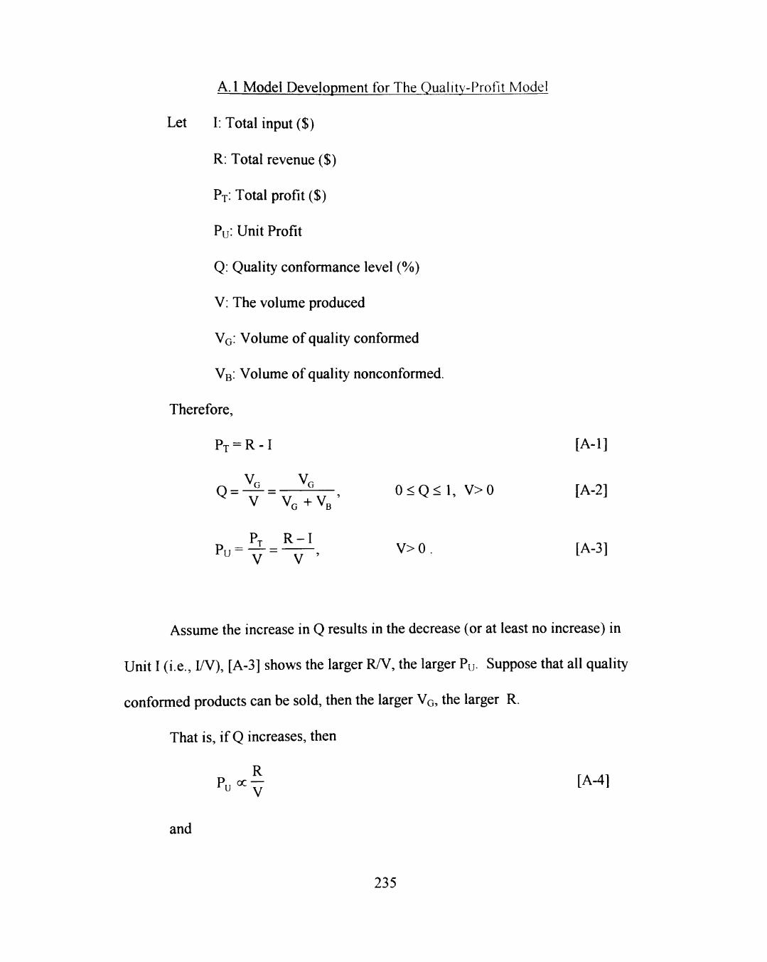
A.l Model Development for The Quaiity-Proflt Model
Let I: Total input ($)
R: Total revenue ($)
PT: Total profit ($)
Pu: Unit Profit
Q: Quality conformance level (%)
V: The volume produced
VQ: Volume of quality conformed
VB: Volume of quality nonconformed.
Therefore,
PT = R - I [A-1]
V V Q = ^ = ^ ^^ , 0 < Q < 1 , V>0 [A-2]
Pu = Y = ^ , V>0. [A-3]
Assume the increase in Q results in the decrease (or at least no increase) in
Unit I (i.e., lA^), [A-3] shows the larger RfV, the larger Pu- Suppose that all quality
conformed products can be sold, then the larger VQ, the larger R.
That is, if Q increases, then
and
235
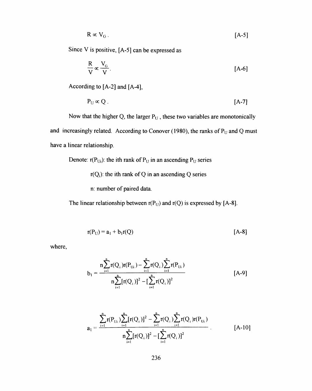
R oc VG . [A-5]
Since V is positive, [A-5] can be expressed as
R V^
According to [A-2] and [A-4],
Pu °c Q . [A-7]
Now that the higher Q, the larger Py , these two variables are monotonically
and increasingly related. According to Conover (1980), the ranks of Pu and Q must
have a linear relationship.
Denote: r(Pui): the ith rank of Pu in an ascending Pu series
r(Qi): the ith rank of Q in an ascending Q series
n: number of paired data.
The linear relationship between r(Pu) and r(Q) is expressed by [A-8].
r(Pu) = ai + b,r(Q) [A-8]
where.
nZr(Q;)r(Pu,)-Zr(Q,)Zr(Pui) i=] i= l_
nZWQ,)f-[Zr(Q,rf b, = ^ = ^ - ^ •^ '^ [A-9]
i=l
£r(Pu, ) I [ r (Q | )f - Zm, )Xr(Q, )r(P„) M M i=l
nZ[>-(Q,)]'-[Zr(Q,)r a, = "^ —„ —. . [A-10]
i = l i = l
236
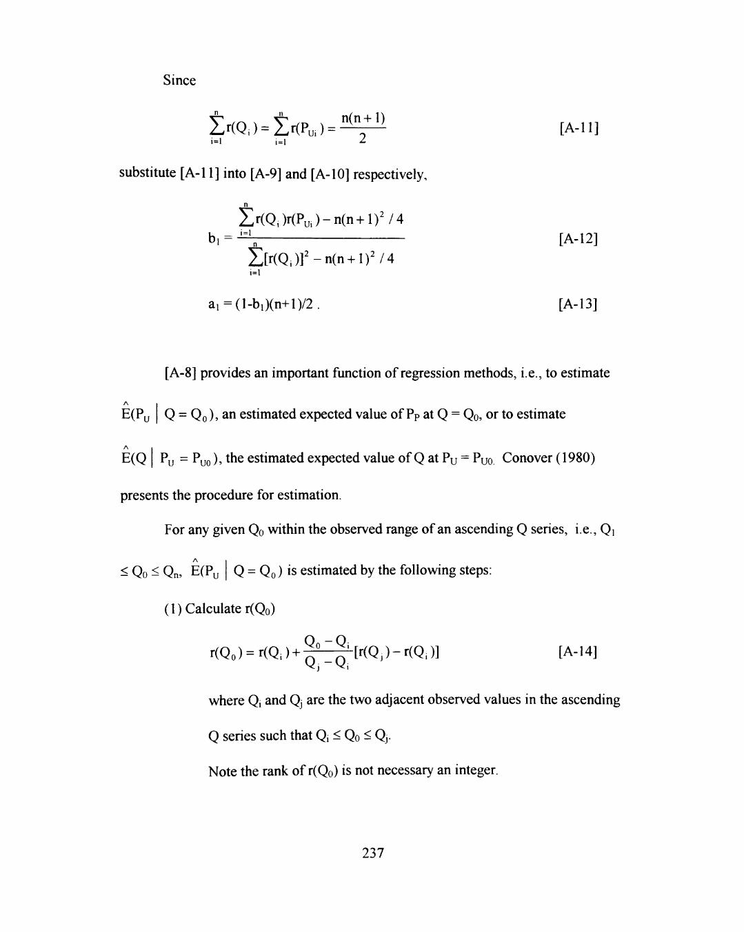
Since
i:r(Q:) = Zr(P„,) = ^ [A-U] i = l i = l ^
substitute [A-11] into [A-9] and [A-10] respectively,
n
Zr(Q.)r(Pu.)-n(n + l ) V 4 i=l
II
Z[r (Q. ) ] ' -n (n +1)^/4 1=1
[A-12]
ai = (l-bi)(n+l)/2. [A-13]
[A-8] provides an important function of regression methods, i.e., to estimate
A
E(Pu Q = Qo), an estimated expected value of Pp at Q = Qo, or to estimate
A
E(Q Py = Puo), the estimated expected value of Q at Pu = Puo Conover (1980)
presents the procedure for estimation. For any given Qo within the observed range of an ascending Q series, i.e., Qi
A
< Qo < Qn, E(Pu Q = Qo) is estimated by the following steps:
(1) Calculate r(Qo)
r(Qo) = r(Q.) + | ^ f | ^ [ r ( Q ^ ) - r ( Q O ] [A-14]
where Qi and Qj are the two adjacent observed values in the ascending
Q series such that Q, < Qo < Qj.
Note the rank of r(Qo) is not necessary an integer.
237

* Do not calculate r(Qo) if Qo is less than the smallest observed Qi
or greater than the largest observed Qn.
(2) Calculate r(Puo)
r(Puo) is calculated by [A-8]. r(Puo) is not necessary an integer.
(3) Calculate E(Pu Q = Qo)
r(Puo)-r(P„i)
r(Pu,)-r(Pu.) E(Pu Q=Qo)-Pu,+:r. ::. :(Pu.-Pu.) [A-IS]
where r(Pui) and r(Puj) are the two adjacent values in the ascending
r(Pu) series such that r(Pui) < r(Puo) < r(Puj).
If r(Puo) is greater than the largest observed rank of Pun, let
A
E(Pu Q = Qo) = r(Pun)- If r(Puo) is less than the smallest observed
rank of Pui, let E(Pu Q = Qo) =r(Pui).
For any given Puo, E(Q P = Puo )is estimated by the folloyving steps:
A
(1) Calculate the two end points, the smallest E(Pu Q = Qj) and the largest
A
E(Pu Q = Qn), according to the preceding procedure.
(2) Calculate each r(Q,) for each r(Pui)
r(Q) = [r(Pu)-a, ] /b, [A-16]
This equation is another form of [A-8].
(3) Convert each r(Q,) to E(Q | P = P .)
238
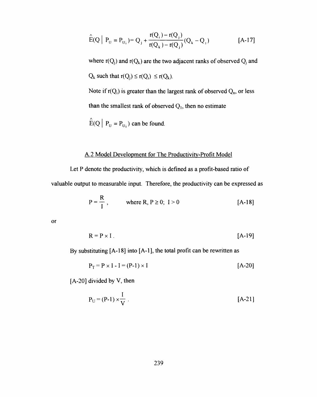
r(Q, - r Q , E(Q P u = R , ) = Q , + • ^ ( Q , - Q ) [A-17]
v^ u u,; Vj r(Qj-r(Qj)^^' ^'^ ^
where r(Qj) and r(Qk) are the two adjacent ranks of observed Qj and
Qk such that r(Qj) < r(Q.) < r(Qk).
Note if r(Q,) is greater than the largest rank of observed Qn, or less
than the smallest rank of observed Qi, then no estimate
A
E(Q Pu = Puj) can be found.
A.2 Model Development for The Productivity-Profit Model
Let P denote the productivity, which is defined as a profit-based ratio of
valuable output to measurable input. Therefore, the productivity can be expressed as
R P = — , where R, P > 0; I > 0 [A-18]
or
R = P x I . [A-19]
By substituting [A-18] into [A-1], the total profit can be rewritten as
PT = P X I - I = ( P - 1 ) X I [A-20]
[A-20] divided by V, then
PU = ( P - 1 ) X ^ - [A-21]
239
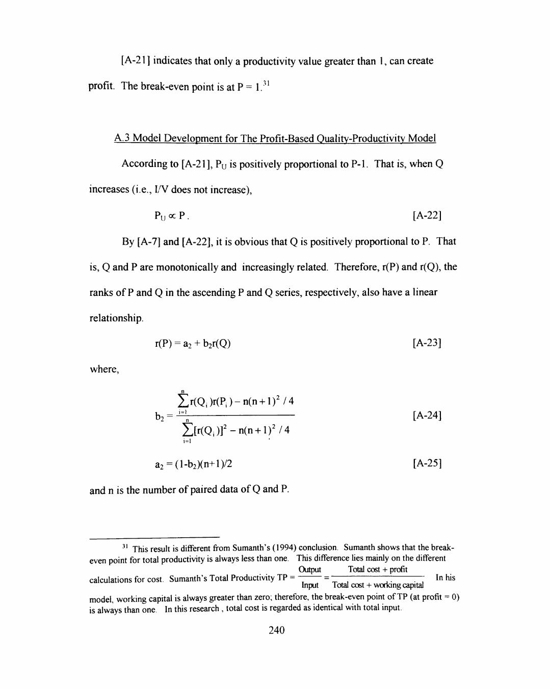
[A-21 ] indicates that only a productivity value greater than 1, can create
profit. The break-even point is at P = 1. '
A. 3 Model Development for The Profit-Based Quality-Productivity Model
According to [A-21], Pu is positively proportional to P-1. That is, when Q
increases (i.e., I/V does not increase),
Pu oc P. [A-22]
By [A-7] and [A-22], it is obvious that Q is positively proportional to P. That
is, Q and P are monotonically and increasingly related. Therefore, r(P) and r(Q), the
ranks of P and Q in the ascending P and Q series, respectively, also have a linear
relationship.
r(P) = a2 + b2r(Q) [A-23]
where,
Zr(Q.)r(P.)-n(n + l ) V 4
b2 = —„ [A-24] Z[r(Qi)] ' -n(n + l ) ' / 4 1=1
a2 = (l-b2)(n+l)/2 [A-25]
and n is the number of paired data of Q and P.
' This result is different from Sumanth's (1994) conclusion. Sumanth shows that the breakeven point for total productivity is always less than one. This difference lies mainly on the different
Output Total cost + profit calculations for cost. Sumanth's Total Productivity TP = - = - — — — In his
Input Total cost + working capital model, working capital is always greater than zero; therefore, the break-even point of TP (at profit = 0) is always than one. In this research , total cost is regarded as identical with total input.
240

[A-23] shows there exists a positive and linear relationship between the ranks
ofproductivity and quality. This linear regression model provides an approach, based
on ranks, to predict productivity P (or quality Q) with a given value Q (or P). The
A
procedure of prediction is similar to the steps of estimating E(Pu Q = Qo) and
A
E(Q Pu = Puo) in the preceding Quality-Profit model.
More specifically, for any given Qo within the observed range of an ascending
A
Q series, E(P Q = Q ) is obtained by the following steps:
(1) Calculate r(Qo)
Using the equation [A-14] and its rule.
(2) Calculate r(Po)
r(Po) is calculated by [A-23]. r(Po) is not necessary an integer.
(3) Calculate E(P I Q = Qo)
r(Po)-r(P.) E(P I Q = Qo)= Pi + ,(p";_,(yj(Pi-Pi) [A-26]
where r(Pi) and r(Pj) are the two adjacent values in the ascending
r(P) series such that r(P,) < r(Po) < r(Pj).
If r(Po) is greater than the largest rank of observed Pn, let
E(P I Q = Qo) = r(Pn)- If r(Po) is less than the.smallest rank of
observed Pi, let E(P Q = Qo)=r(P,).
241
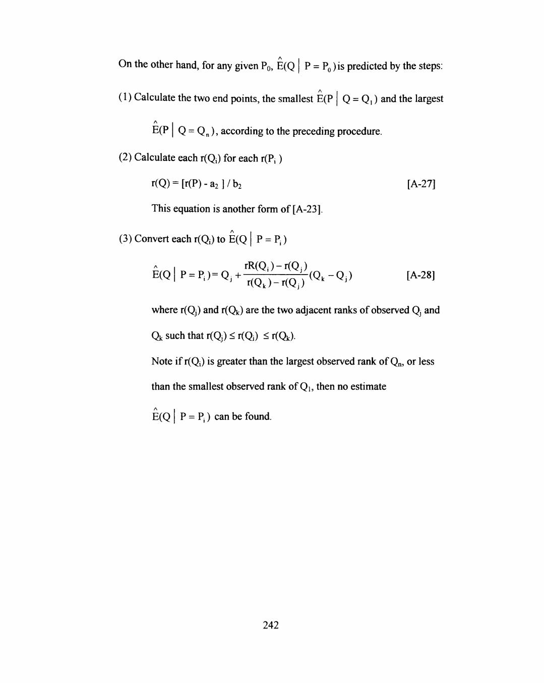
On the other hand, for any given Po, E(Q P = PQ ) is predicted by the steps
(1) Calculate the two end points, the smallest E(P Q = Q,) and the largest
E(P Q = Q ) according to the preceding procedure.
(2) Calculate each r(Q,) for each r(P,)
r(Q) = [r(P) - a2 ] / b2
This equation is another form of [A-23].
[A-27]
(3) Convert each r(Q,) to E(Q P = Pj)
- I rRQ. -r(QJ E(Q P = P.)=Q.+ • ^ ^ ( Q , - Q )
' ' ' rQ,)-r(Q^)^'^'^ ^^^ [A-28]
where r(Qj) and r(Qk) are the two adjacent ranks of observed Qj and
Qk such that r(Q) < r(QO < r(Qk).
Note if r(Qi) is greater than the largest observed rank of Qn, or less
than the smallest observed rank of Qi, then no estimate
E(Q P = Pi) can be found.
242

APPENDIX B
QUALITY INSPECTION POINTS IN ABC AND XYZ COMPANIES
243
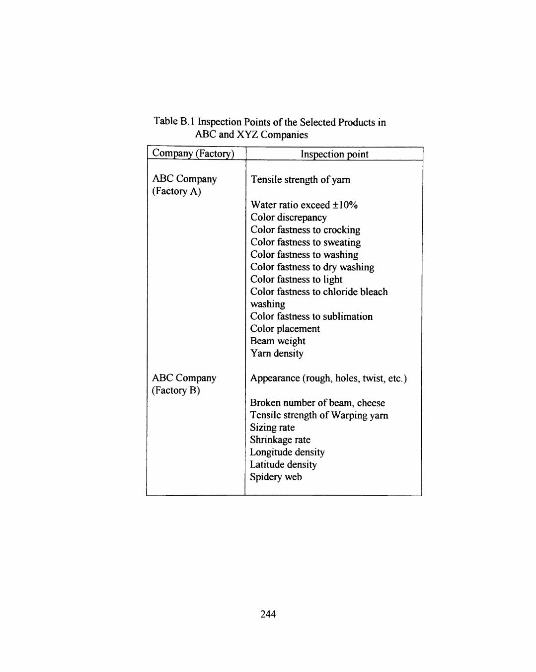
Table B.l Inspection Points ofthe Selected Products in ABC and XYZ Companies
Company (Factory)
ABC Company (Factory A)
ABC Company (Factory B)
Inspection point
Tensile strength of yam
Water ratio exceed ±10% Color discrepancy Color fastness to crocking Color fastness to sweating Color fastness to washing Color fastness to dry washing Color fastness to light Color fastness to chloride bleach washing Color fastness to sublimation Color placement Beam weight Yam density
Appearance (rough, holes, twist, etc.)
Broken number of beam, cheese Tensile strength of Warping yam Sizing rate Shrinkage rate Longitude density Latitude density Spidery web
244
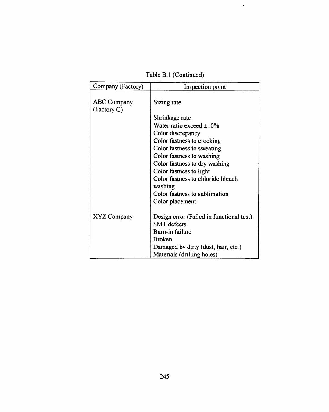
Table B.l (Continued)
Company (Factory)
ABC Company (Factory C)
XYZ Company
Inspection point
Sizing rate
Shrinkage rate Water ratio exceed ±10% Color discrepancy Color fastness to crocking Color fastness to sweating Color fastness to washing Color fastness to dry washing Color fastness to light Color fastness to chloride bleach washing Color fastness to sublimation Color placement
Design error (Failed in functional test) SMT defects Bum-in failure Broken Damaged by dirty (dust, hair, etc.) Materials (drilling holes)
245

APPENDIX C
TABLE FOR THE SPEARMAN'S RHO TEST
246

Table C l Quantiles ofthe Spearman Test Statistic (Source: Conover,1980, p. 456)
n
4 5 6 7 8 9 10 11 12 13 14 15 16 17 18 19 20 21 22 23 24 25 26 27 28 29 30
p=.900
.800
.7000
. 000 .5357
.5000
.4667
.4424
.4182
.3986
.3791
.3626
.3500
.3382
.3260
.3148
.3070
.2977
.2909
.2829
.2767
.2704
.2646
.2588
.2540
.2490
.2443
.2400
.950
.800
.8000
.7714
.6768
.6190
.5833
.5515
.5273
.4965 4780 .4593 4429 .4265 .4118 .3994 .3895 .3789 .3688 .3597 .3518 .3435 .3362 .3299 .3236 .3175 .3113 .3059
.975
.9000
.8286
.7450
.7143
.6833
.6364
.6091
.5804
.5549
.5341
.5179
.5000 4853 4716 4579 4451 4351 4241 4150 .4061 .3977 .3894 .3822 .3749 .3685 .3620
.990
.9000
.8857
.8571
.8095
.7667
.7333
.7000
.6713
.6429
.6220
.6000
.5824
.5637
.5480
.5333
.5203
.5078
.4963 4852 .4748 .4654 4564 .4481 .4401 .4320 .4251
.995
.9429
.8929
.8571
.8167
.7818
.7455
.7273
.6978
.6747
.6536
.6324
.6152
.5975
.5825
.5684
.5545
.5426
.5306
.5200
.5100
.5002
.4915
.4828 4744 .4665
.999
.9643
.9286
.9000
.8667
.8364
.8182
.7912
.7670
.7464
.7265
.7083
.6904
.6737
.6586
.6455
.6318
.6186
.6070
.5962
.5856
.5757
.5660
.5567
.5479
For n greater than 30 the appropriate quantiles of p may be obtained from
where X is the p quantile of a standard normal random variable obtained from the normal distribution
table. The entries in this table are selected quantiles w^ ofthe Spearman rank correlation coefficient
p when used as a test statistic. The lower quantiles may be obtained from the equation
The critical region corresponds to values of p smaller than (or greater than) but not including the appropriate quantile. Note that the median of p is 0.
247

APPENDK D
RESULTS OF THE LILLIEFORTS NORMALITY TESTS
248
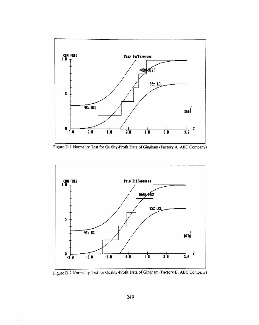
CUH FREQ 1.8 T
Pail* Diffepences
. 5 •-
-3.8
DAT /
3.8
Figure D. 1 Normality Test for Quality-Profit Data of Gingham (Factory A, ABC Company)
CUH niEQ 1.8 T
Palp Diffennces
. 5 ••
3.8 -2.8
DATi /
3.8
Figure D.2 Normality Test for Quality-Profit Data of Gingham (Factory B, ABC Company)
249
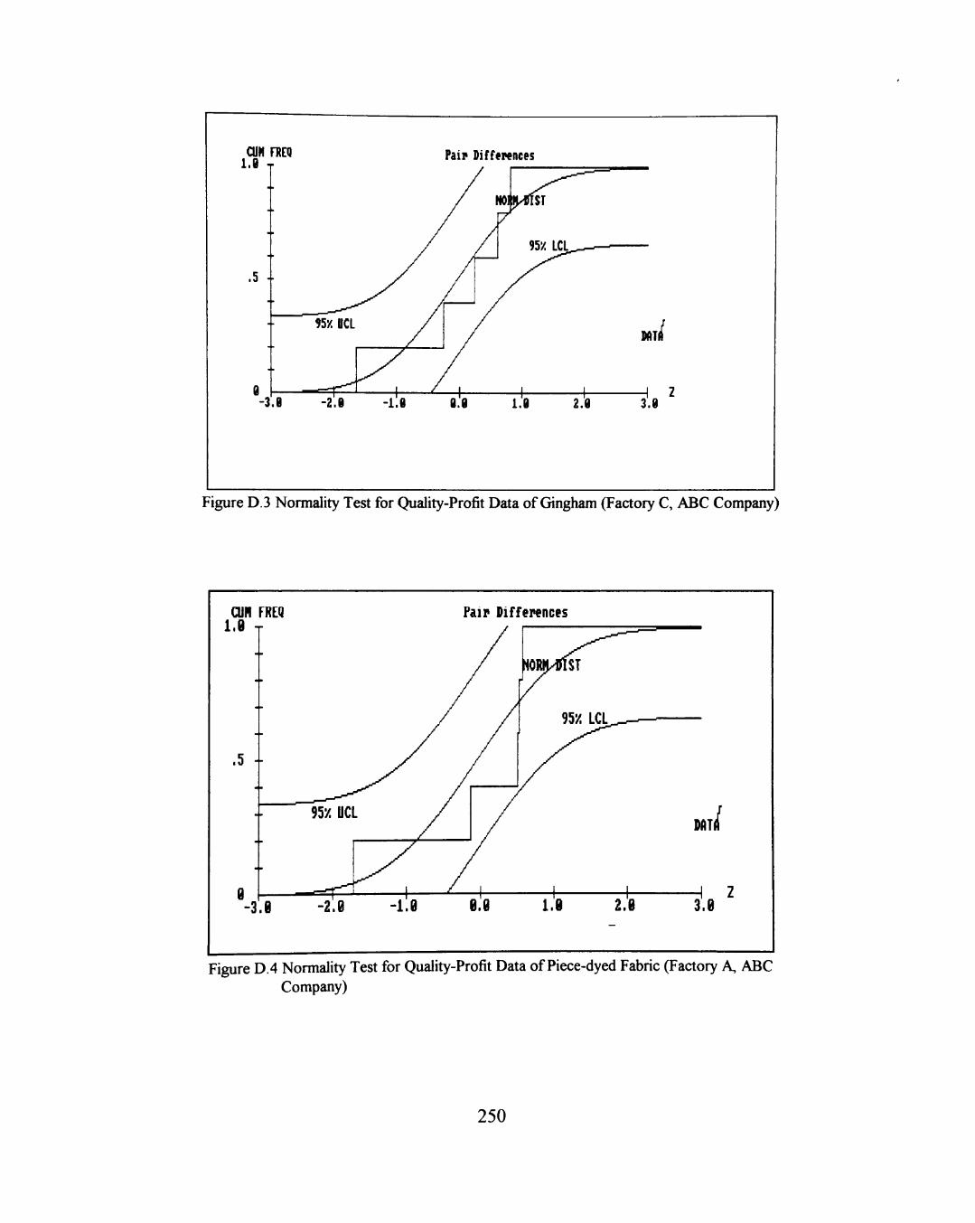
CUH FREQ i.e T
Pair Differences
.5 -
-3.8 -2.0
MTi i
3.8
Figure D.3 Normality Test for Quality-Profit Data of Gingham (Factory C, ABC Company)
CUn FREQ 1.8 T
Paip Diffepences
.5 --
-3.8
DATi /
3.8
Figure D.4 Normality Test for Quality-Profit Data of Piece-dyed Fabric (Factory A, ABC Company)
250
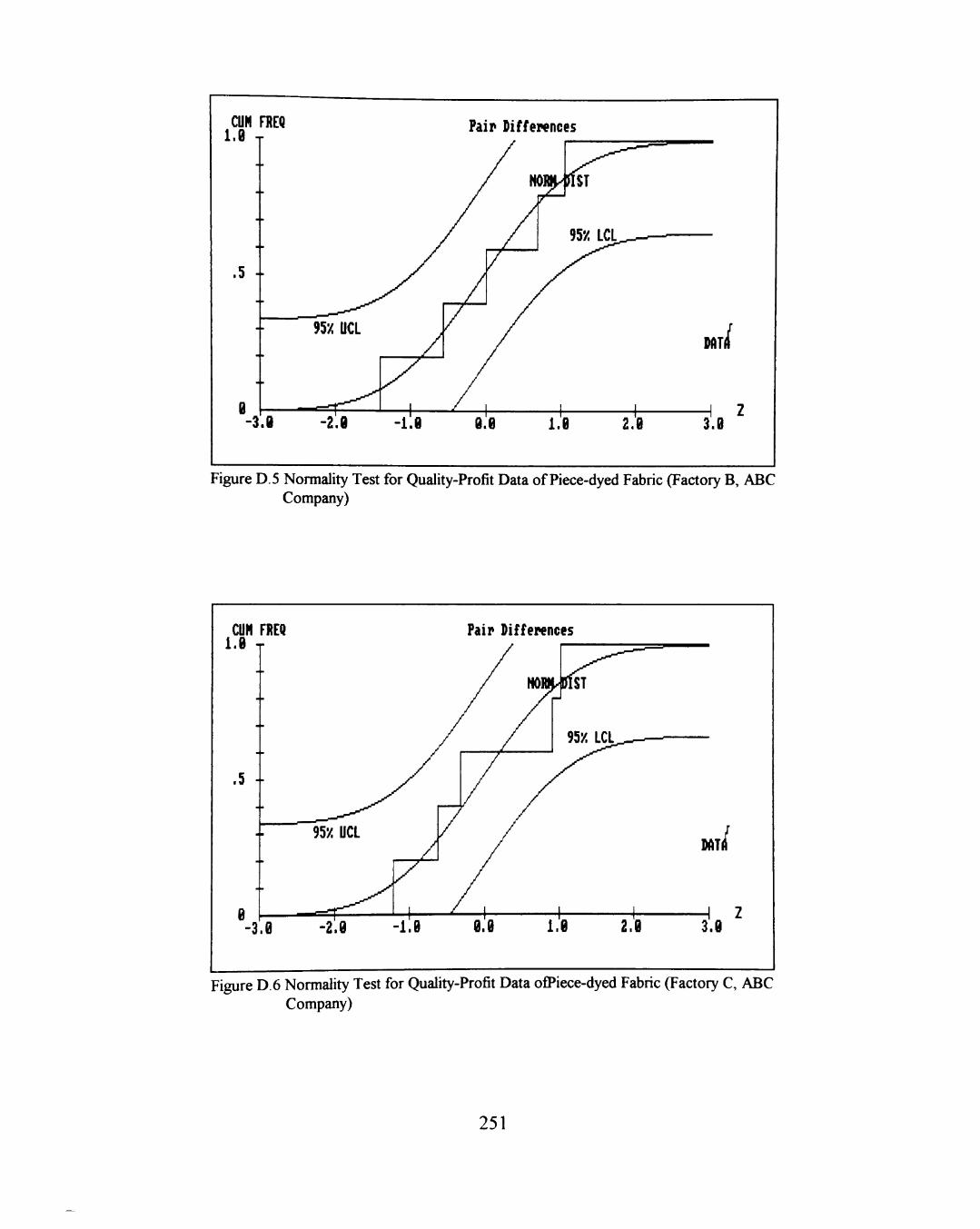
CUN 1.8 n
.5 -
Q
-3
FREQ
.8
95X UCL
-2.8 1
-I1B
Paip Diffepences
/ /
/
/
rfST
73/. L\»L^^^-- '
1 i 1 8.8 1.8 2.'8
MT((
1 2 3.8
Figure D . 5 Normality Test for Quality-Profit Data o f Piece-dyed Fabric (Factory B , A B C Company)
CUH FREQ 1.8 T
Paip Diffepences
.5 -
-3.8
DAT /
3.8
Figure D.6 Normality Test for Quality-Profit Data ofPiece-dyed Fabric (Factory C, ABC Company)
251
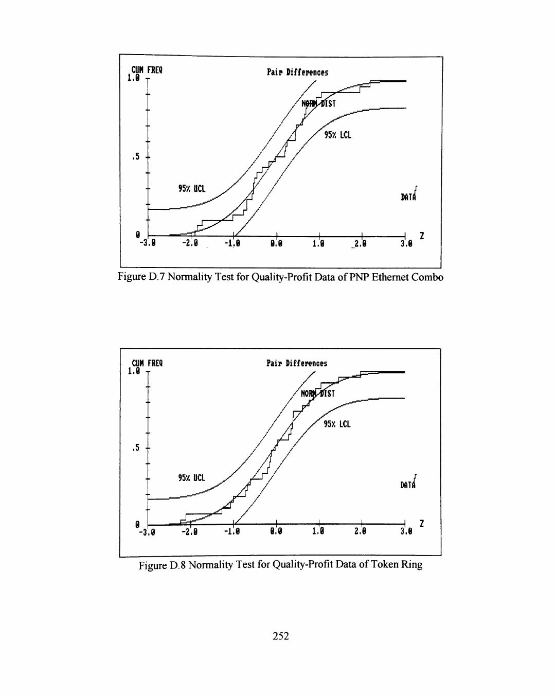
CUH FREQ 1.8 T
Paip Differences
.5 -.
-3.8
DAT /
3.8
Figure D.7 Normality Test for Quality-Profit Data of PNP Ethernet Combo
CUH FREQ 1.8 T
Paip Differences
.5 "
DAT I
3.8 -2.8 -1.8 3.8
Figure D.8 Normality Test for Quality-Profit Data of Token Ring
252

CUH 1.8 1
.5 -
Q
-3
FREQ
.8
m UCL
-2.8
/
1 y -IIB
Pair 1 )iffepences
/
m^
7 0 / . L\^L^_-—1 •-
1 1 1 8.'8 l.'e _2.'8
DATll
1 2 3'. 8
Figure D.9 Normality Test for Productivity-Profit Data of Gingham (Factory A, ABC Company
CUH FREQ 1.8 T
Paip Diffepences
.5 "
-3.8 I Z
Figure D. 10 Normality Test for Productivity-Profit Data of Gingham (Factory B, ABC Company)
253
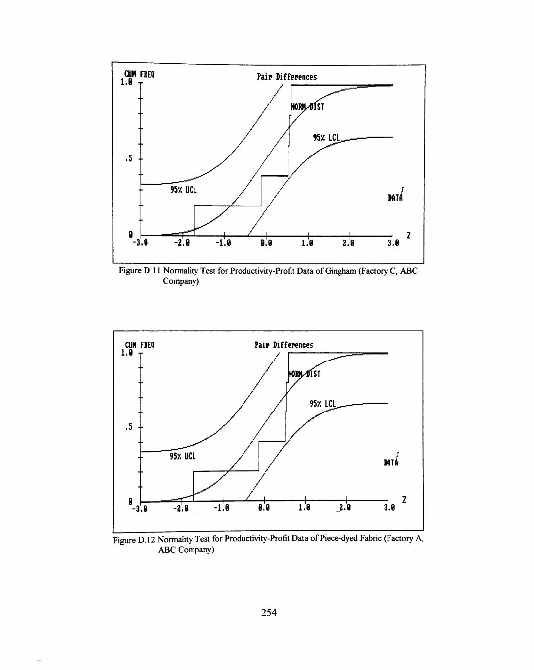
CUH FBEQ 1 . 8 T
Pair Diffepences
.5 "
-3.8
DAT /
3.8
Figure D . 11 Normal i ty Test for Productivity-Profit Data o f Gingham (Factory C, A B C Company)
CUH FREQ 1 .8 T
Paip Diffepences
. 5 ••
-3.8
DAT i
3.8
Figure D. 12 Normality Test for Productivity-Profit Data of Piece-dyed Fabric (Factory A, ABC Company)
254
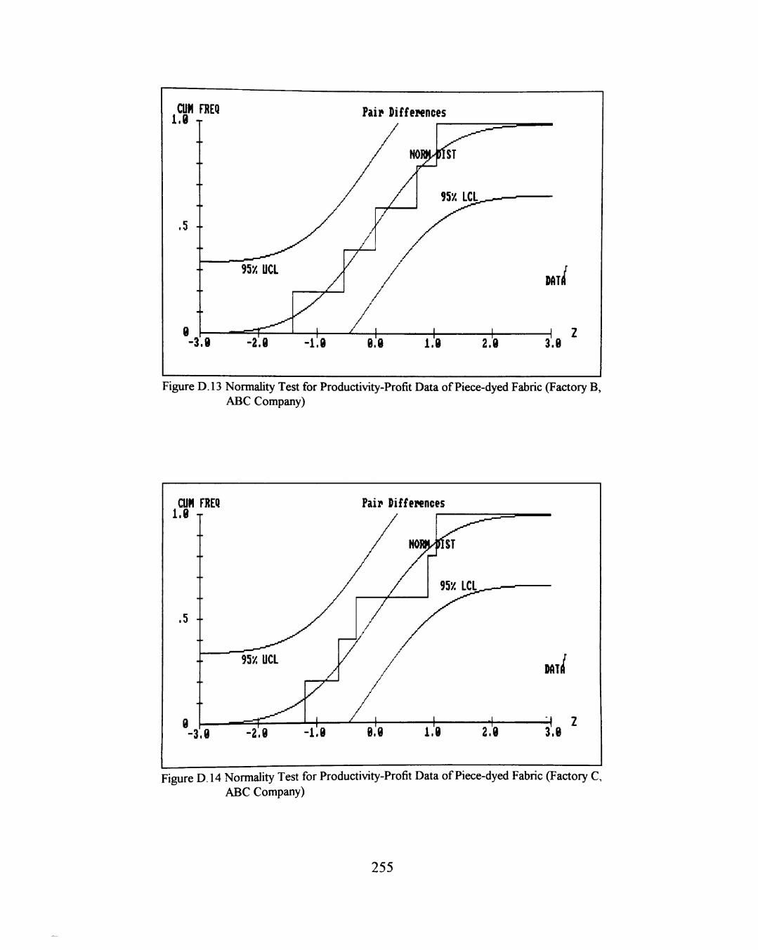
CUH FREQ 1.8 T
Paip Differences
.5 -
-3.8
DAT /
3.8
Figure D.13 Normality Test for Productivity-Profit Data of Piece-dyed Fabric (Factory B, ABC Company)
CUH FREQ 1.8 T
Paip Diffepences
.5 -•
-3.8
DAT /
-2.8 -1.8 3.8
Figure D. 14 Normality Test for Productivity-Profit Data of Piece-dyed Fabric (Factory C, ABC Company)
255
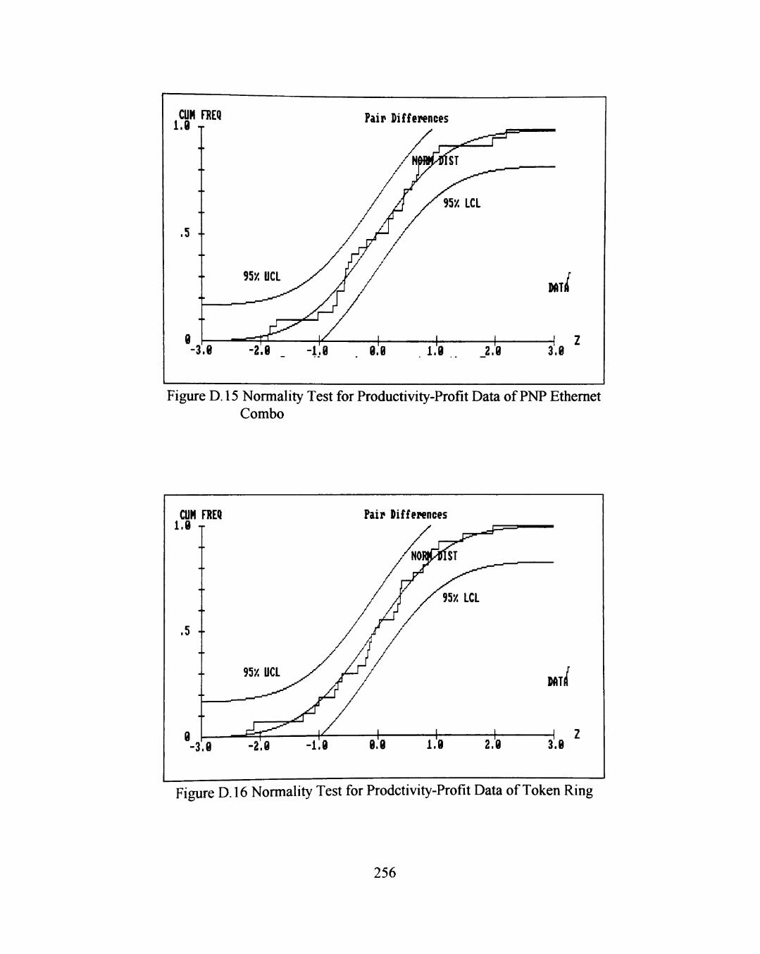
CUH FREQ 1.8 T
Pair Differences
. 5 ••
8 -3.8
DAT /
3.8
Figure D. 15 Normality Test for Productivity-Profit Data of PNP Ethernet Combo
CUH FREQ 1.8 T
Pair Differences
.5 "
DAT /
- ^ - 3 . 8 -2 .8 -1 .8 3.8
Figure D. 16 Normality Test for Prodctivity-Profit Data of Token Ring
256
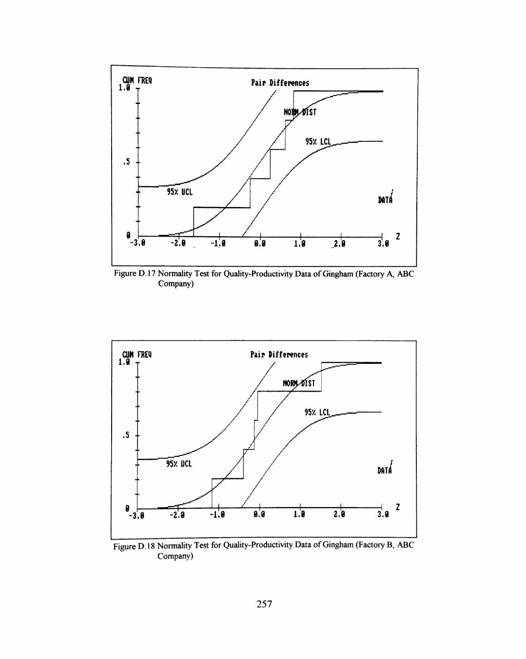
Figure D. 17 Normality Test for Quality-Productivity Data of Gingham (Factory A, ABC Company)
CUH FREQ 1 Q ^ 1 .0 "
. 5 •
8 -3
95>: UCL
.8 -2'. 8
/
1 J
lie
Pi
/
lir Differences
/ NORjHrfST
/ 95Z I ri . \ » L j _ , ^
1 1 1 8.8 1.8 2.8
DAT/
1 2 3.8
Figure D. 18 Normality Test for Quality-Productivity Data of Gingham (Factory B, ABC Company)
257
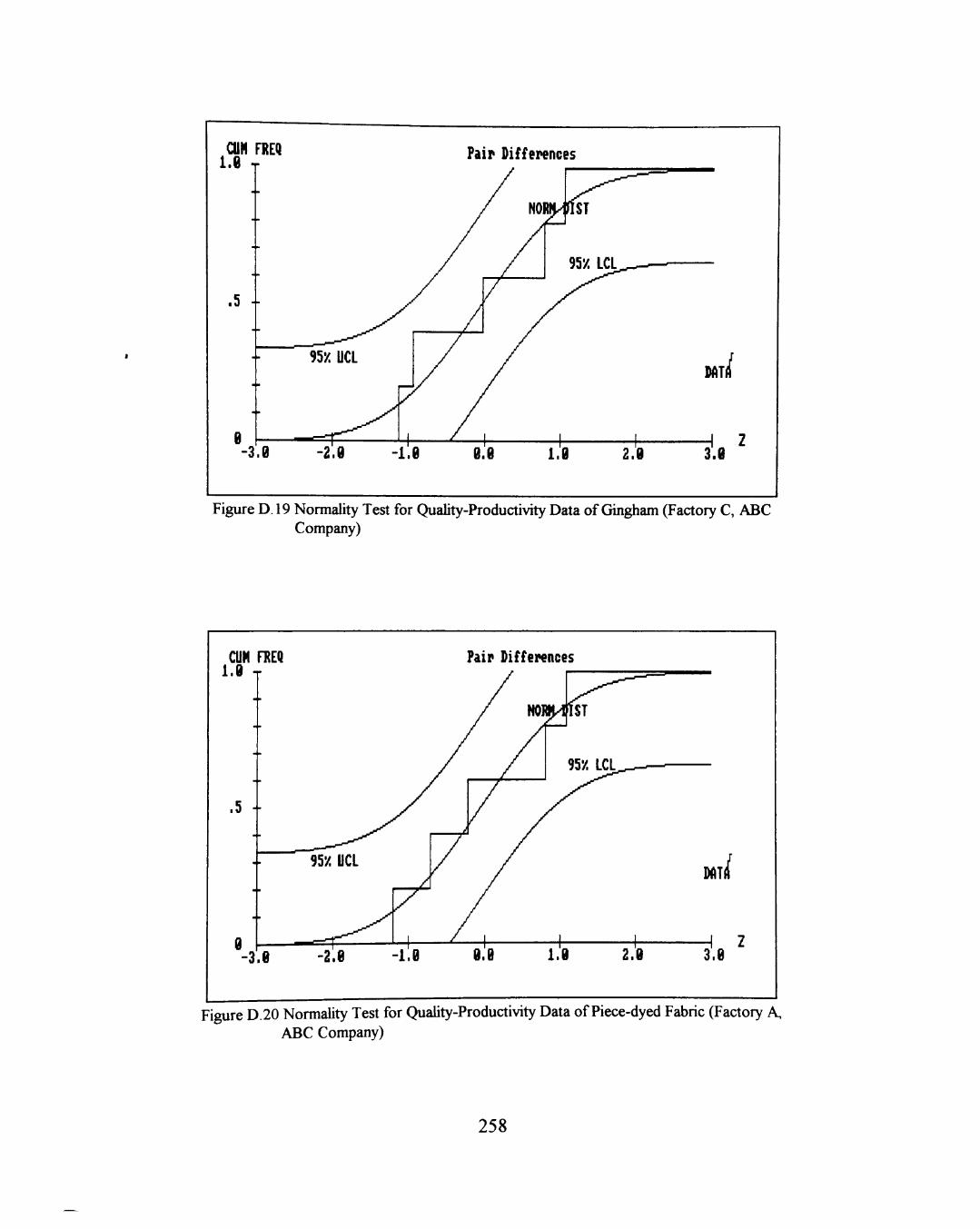
CUH FREQ 1.8 T
. 5 •-
-3.8
DATi /
3.8
Figure D. 19 Normality Test for Quality-Productivity Data of Gingham (Factory C, ABC Company)
CUH FREQ 1 B T-1 . D
.5 -
8 -3 .8
95/. UCL
-2.8
Pair Differences
/ NOT
/ /
, _ i
y / /
»M
3J/. LLL^-—1 ^
/ 1 1 1
- l l8 8.8 l.'e 2.8
mi
1 2 3.8
Figure D.20 Normality Test for Quality-Productivity Data of Piece-dyed Fabric (Factory A, ABC Company)
258
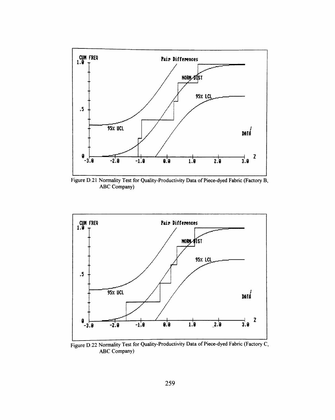
CUH FREQ 1.8 T
.5 -
-3.8
Pair Differences
DAT /
3.8
Figure D.21 Normality Test for Quality-Productivity Data of Piece-dyed Fabric (Factory B, ABC Company)
CUH FUEQ 1 fl ^
. 5 •
8 -3 .8
95X UCL
-2 .8 1 /
-lie
Fair Differences
^
y
NOBH
/
m
95Z L C L ^ ^ ^
1 1 1 8.8 1.8 J.'8
mi
1 2 3.8
Figure D.22 Normality Test for Quality-Productivity Data of Piece-dyed Fabric (Factory C, ABC Company)
259
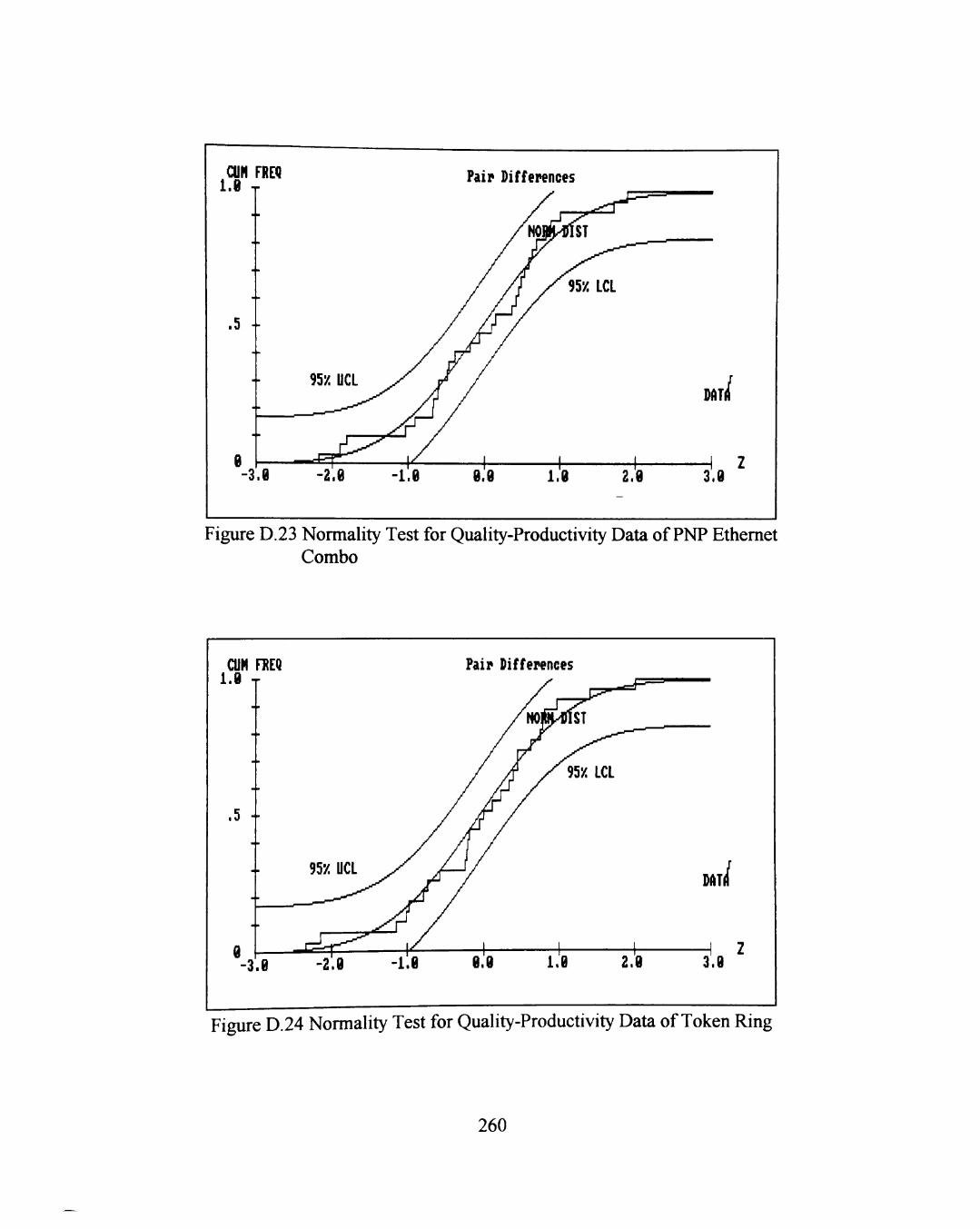
CUH FREQ 1.8 T
Pair Differences
.5 --
-3.8
DAT /
3.8
Figure D.23 Normality Test for Quality-Productivity Data of PNP Ethernet Combo
CUH FltEQ 1.8 T
Pair Differences
. 5 ••
8 -3.8 -2.8
DAT /
3.8
Figure D.24 Normality Test for Quality-Productivity Data of Token Ring
260

APPENDIX E
A PROOF FOR THE RELATIONSHIP BETWEEN SLOPE OF A REGRESSION
LINE BASED ON RANKS AND ITS CORRELATION COEFFICIENT
261
Let
X : independent variable.
Y: dependent variable
r(XO:theithrankofXi
r(Y,): the ith rank of Y,
n : number of paired data (X, Y).
According to Eqs. [A-8] and [A-12] in the Appendix A,
r(Y) = a + br(X) [E-1]
where
n
Zr(X.)r(Y.)-n(n +1)^/4 b = ^ ; . [E-2]
£ [ r (X . ) ] ' - n (n+1)^ /4 i=l
When sample data have no ties,
^ , ^ , n(n + l)(2n + l) Z[r(X. )f = Z[r(Y. )f = ^ . [E-3] i = l i = I "
Substitute [E-3] into [E-2],
12ir(X,)r(Y,)-3n(n + l ) '
n(n -1 )
On the other hand, according to Eq. [4-1] of section 4.3.1.1,
where
262
or
T = Z[r(X,)-r(Y,)f [E-6] i = l
=Z[r(X, )f - 2Zr(X. )r(Y,) +X[r(X)]') • [E-7] 1=1 i = l i = l
n 2 n 2
Again, replace Sr(X.) and XKYJ ) by [E-3], yields i = l 1=1
^^(A7 + l ) ( 2 ^ + l ) ^ , V N . V ^ T 22^r(X, )r(Y,)
i=l
i=l
Substitute [E-9] into [E-4],
[E-10] equals [E-5]. Therefore, b = p when there are no ties.
263
[E-8]
n
12Zr(Xi)r(Y,) = 2n(n + l)(2n+l)-6T . [E-9]
2n(n + l)(2n + l)-6T-3n(n + l)^ ' ' " n(n^-l)
= l - - 4 ^ [E-10] n(n -1)

APPENDIX F
THE DURBIN-WATSON TEST PROCEDURE AND ITS TABLE
264
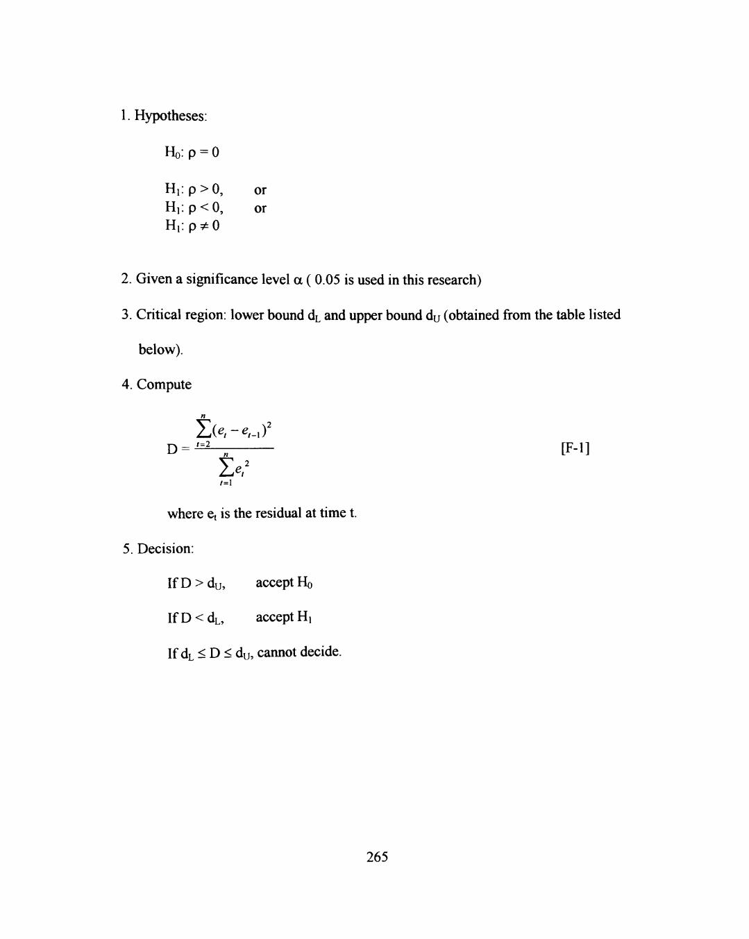
1. Hypotheses:
Ho:p = 0
Hi:p>0, or Hi:p<0, or Ui'.Q^O
2. Given a significance level a ( 0.05 is used in this research)
3. Critical region: lower bound dL and upper bound du (obtained from the table listed
below).
4. Compute
D = -'^2__ [F-l] 1=2 n
t=l
where et is the residual at time t.
5. Decision:
IfD>du, accept Ho
IfD<dL, accept Hi
If dL < D < du, cannot decide.
265
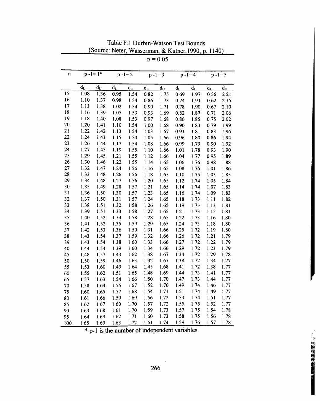
Table F. 1 Durbin-Watson Test Bounds (Source: Neter, Wasserman, & Kutner,1990, p. 1140)
a = 0.05
n p - l = l * p - l = 2 p - l = 3 p - l = 4 p - l = 5
15 16 17 18 19 20 21 22 23 24 25 26 27 28 29 30 31 32 33 34 35 36 37 38 39 40 45 50 55 60 65 70 75 80 85 90 95 100
du 1.08
1.10
1.13
1.16 1.18
1.20
1.22 1.24 1.26 1.27
1.29
1.30 1.32 1.33 1.34
1.35 1.36 1.37 1.38 1.39
1.40 1.41
1.42 1.43 1.43 1.44
1.48 1.50
1.53 1.55
1.57
1.58
1.60
1.61
1.62 1.63
1.64
1.65
du 1.36
1.37
1.38 1.39
1.40 1.41
1.42 1.43 1.44
1.45
1.45 1.46 1.47 1.48 1.48 1.49 1.50 1.50 1.51
1.51 1.52
1.52 1.53 1.54
1.54 1.54 1.57
1.59 1.60
1.62 1.63 1.64
1.65 1.66
1.67
1.68 1.69
1.69
dL 0.95
0.98
1.02 1.05 1.08 1.10
1.13 1.15 1.17
1.19 1.21
1.22 1.24 1.26 1.27
1.28 1.30
1.31 1.32 1.33 1.34 1.35 1.36 1.37 1.38 1.39
1.43 1.46 1.49
1.51 1.54
1.55 1.57
1.59
1.60
1.61
1.62 1.63
du 1.54
1.54
1.54 1.53 1.53 1.54
1.54 1.54 1.54
1.55 1.55 1.55 1.56 1.56 1.56 1.57
1.57 1.57
1.58 1.58 1.58 1.59 1.59 1.59 1.60 1.60 1.62 1.63 1.64
1.65 1.66 1.67
1.68
1.69 1.70
1.70
1.71
1.72
du 0.82
0.86 0.90
0.93 0.97 1.00
1.03 1.05 1.08
1.10 1.12 1.14 1.16 1.18 1.20 1.21 1.23 1.24 1.26 1.27 1.28 1.29 1.31 1.32 1.33 1.34 1.38 1.42 1.45 1.48 1.50
1.52 1.54
1.56 1.57
1.59
1.60 1.61
du 1.75
1.73 1.71
1.69 1.68 1.68 1.67 1.66
1.66 1.66 1.66 1.65 1.65 1.65 1.65 1.65 1.65 1.65 1.65
1.65 1.65 1.65 1.66 1.66 1.66 1.66 1.67 1.67
1.68 1.69 1.70 1.70
1.71
1.72 1.72 1.73
1.73 1.74
du 0.69
0.74
0.78
0.82 0.86 0.90 0.93 0.96 0.99 1.01
1.04 1.06 1.08 1.10 1.12 1.14
1.16 1.18 1.19
1.21 1.22 1.24 1.25 1.26 1.27
1.29 1.34 1.38 1.41 1.44
1.47 1.49
1.51 1.53 1.55
1.57
1.58 1.59
du 1.97
1.93
1.90 1.87
1.85 1.83 1.81 1.80 1.79
1.78 1.77 1.76 1.76 1.75 1.74 1.74 1.74 1.73 1.73 1.73 1.73 1.73 1.72 1.72 1.72 1.72 1.72 1.72 1.72 1.73 1.73 1.74
1.74 1.74
1.75 1.75 1.75
1.76
du 0.56
0.62
0.67 0.71
0.75 0.79 0.83 0.86 0.90
0.93 0.95 0.98 1.01 1.03 1.05 1.07 1.09
1.11 1.13
1.15 1.16 1.18 1.19 1.21 1.22 1.23 1.29 1.34 1.38 1.41 1.44
1.46 1.49
1.51 1.52
1.54 1.56 1.57
du 2.21
2.15
2.10
2.06 2.02 1.99
1.96 1.94 1.92
1.90 1.89
1.88 1.86 1.85 1.84 1.83 1.83 1.82
1.81 1.81 1.80 1.80 1.80 1.79 1.79
1.79 1.78 1.77 1.77 1.77 1.77
1.77
1.77 1.77
1.77 1.78
1.78 1.78
p-1 is the number of independent variables
266
APPENDDC G
PREDICTED VALUES OF SPECIFIC MODELS OF QUALITY-PROFIT
RELATIONSHIP
267
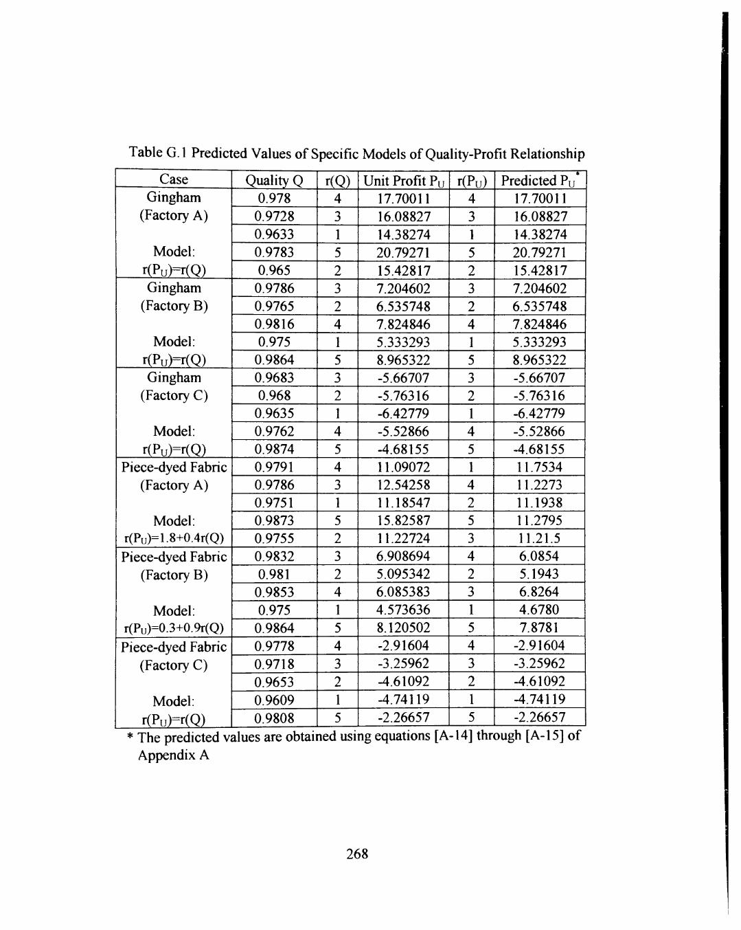
Table G.l Predicted Values of Specific Models of Quality-Profit Relationship
Case Gingham
(Factory A)
Model: r(Pu)=r(0) Gingham
(Factory B)
Model: r(Pu)=r(0) Gingham
(Factory C)
Model: r(Pu)=r(Q)
Piece-dyed Fabric (Factory A)
Model: r(Pu)=1.8+0.4r(Q) Piece-dyed Fabric
(Factory B)
Model: r(Pu)=0.3+0.9r(Q) Piece-dyed Fabric
(Factory C)
Model: r(PH)=r(Q)
Quality Q 0.978
0.9728 0.9633 0.9783 0.965 0.9786 0.9765 0.9816 0.975
0.9864 0.9683 0.968
0.9635 0.9762 0.9874 0.9791 0.9786 0.9751 0.9873 0.9755 0.9832 0.981
0.9853 0.975
0.9864 0.9778 0.9718 0.9653 0.9609 0.9808
r(Q) 4 3 1 5 2 3 2 4 1 5 3 2 1 4 5 4 3 1 5 2 3 2 4 1 5 4 3 2 1 5
Unit Profit Pu 17.70011 16.08827 14.38274 20.79271 15.42817 7.204602 6.535748 7.824846 5.333293 8.965322 -5.66707 -5.76316 -6.42779 -5.52866 -4.68155 11.09072 12.54258 11.18547 15.82587 11.22724 6.908694 5.095342 6.085383 4.573636 8.120502 -2.91604 -3.25962 -4.61092 -4.74119 -2.26657
r(Pn) 4 3 1 5 2 3 2 4 1 5 3 2 1 4 5 1 4 2 5 3 4 2 3 1 5 4 3 2 1 5
Predicted Pu' 17.70011 16.08827 14.38274 20.79271 15.42817 7.204602 6.535748 7.824846 5.333293 8.965322 -5.66707 -5.76316 -6.42779 -5.52866 -4.68155 11.7534 11.2273 11.1938 11.2795 11.21.5 6.0854 5.1943 6.8264 4.6780 7.8781
-2.91604 -3.25962 -4.61092 -4.74119 -2.26657
* The predicted values are obtained using equations [A-14] through [A-15] of Appendix A
268
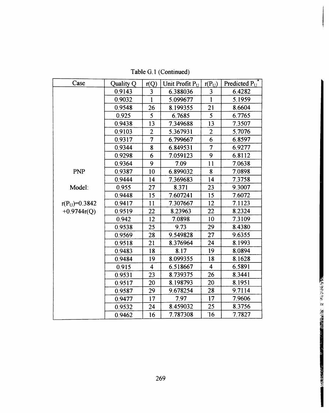
T a b l e d (Continued)
Case
PNP
Model:
r(Pu)=0.3842
+0.9744r(Q)
Quality Q 0.9143 0.9032
0.9548 0.925 0.9438
0.9103 0.9317 0.9344 0.9298 0.9364 0.9387 0.9444 0.955 0.9448 0.9417 0.9519 0.942 0.9538 0.9569 0.9518 0.9483 0.9484 0.915 0.9531 0.9517 0.9587
0.9477 0.9532
0.9462
r(Q) 3 1 26 5 13 2 7 8 6 9 10 14 27 15 11 22 12 25 28 21 18 19 4 23 20 29 17 24
16
Unit Profit Pu 6.388036 5.099677 8.199355 6.7685 7.349688 5.367931 6.799667 6.849531
7.059123 7.09
6.899032 7.369683 8.371
7.607241 7.307667 8.23963 7.0898 9.73
9.549828 8.376964 8.17
8.099355 6.518667 8.739375 8.198793 9.678254 7.97
8.459032
7.787308
r(Pu) 3 1
21 5 13 2 6 7
9
11 8 14 23 15 12 22 10 29 27 24 19 18 4 26 20 28 17 25
16
Predicted Pu' 6.4282 5.1959 8.6604
6.7765 7.3507 5.7076 6.8597 6.9277
6.8112
7.0638 7.0898 7.3758 9.3007 7.6072 7.1123 8.2324 7.3109 8.4380 9.6355 8.1993 8.0894 8.1628 6.5891 8.3441 8.1951 9.7114
7.9606 8.3756 7.7827
"^
:v.ti
269 tE
I
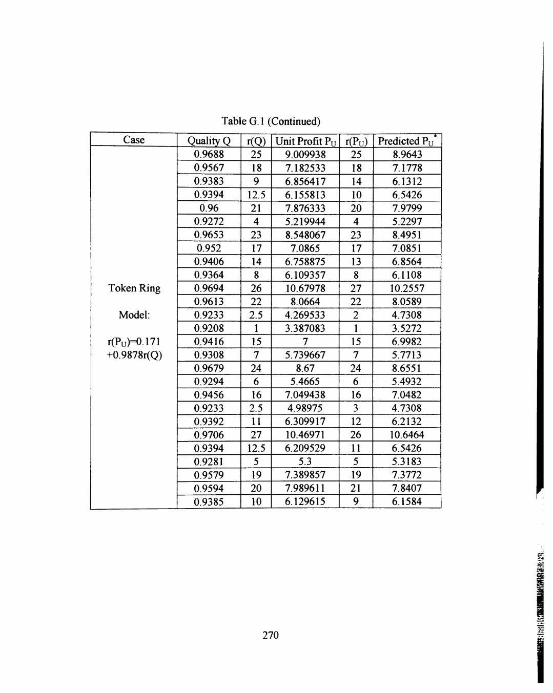
Table G. 1 (Continued)
Case
Token Ring
Model:
r(Pu)=0.171 +0.9878r(Q)
Quality Q 0.9688 0.9567
0.9383 0.9394 0.96 0.9272 0.9653 0.952 0.9406 0.9364 0.9694 0.9613 0.9233 0.9208 0.9416 0.9308 0.9679 0.9294 0.9456 0.9233 0.9392 0.9706 0.9394 0.9281 0.9579 0.9594 0.9385
r(Q) 25
18 9
12.5 21 4 23 17 14 8 26 22 2.5 1 15 7 24 6 16 2.5 11 27 12.5 5 19 20
10
Unit Profit Pu 9.009938
7.182533 6.856417 6.155813 7.876333 5.219944 8.548067 7.0865
6.758875 6.109357 10.67978 8.0664
4.269533 3.387083
7 5.739667 8.67
5.4665 7.049438 4.98975 6.309917 10.46971 6.209529
5.3 7.389857 7.989611 6.129615
r(Pu) 25 18 14 10 20 4 23 17 13 8 27 22 2 1 15 7 24 6 16 3 12 26 11 5 19 21 9
Predicted Pu' 8.9643
7.1778 6.1312 6.5426 7.9799 5.2297 8.4951 7.0851 6.8564 6.1108 10.2557 8.0589 4.7308 3.5272 6.9982 5.7713 8.6551 5.4932 7.0482 4.7308
6.2132 10.6464 6.5426 5.3183 7.3772 7.8407 6.1584
^ ?&
270 ^
APPENDIX H
PREDICTED VALUES OF SPECIFIC MODELS OF QUALITY-PRODUCTIVITY
RELATIONSHIP
271
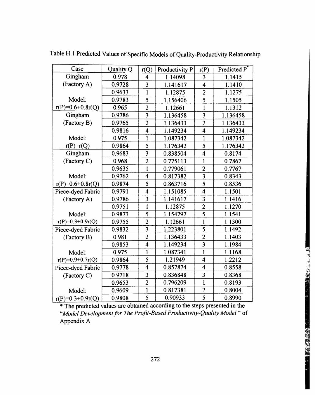
Table H. 1 Predicted Values of Specific Models of Quality-Productivity Relationship
Case Gingham
(Factory A)
Model: r(P)=0.6+0.8r(Q)
Gingham (Factory B)
Model: r(P)=r(Q) Gingham
(Factory C)
Model: r(P)=0.6+0.8r(Q) Piece-dyed Fabric
(Factory A)
Model: r(P)=0.3+0.9r(Q)
Piece-dyed Fabric (Factory B)
Model: r(P)=0.9+0.7r(Q)
Piece-dyed Fabric (Factory C)
Model: r(P)=0.3+0.9r(Q)
Quality Q 0.978
0.9728 0.9633 0.9783 0.965 0.9786 0.9765 0.9816 0.975
0.9864 0.9683 0.968
0.9635 0.9762 0.9874 0.9791 0.9786 0.9751 0.9873 0.9755 0.9832 0.981 0.9853 0.975
0.9864 0.9778 0.9718 0.9653 0.9609 0.9808
r(Q) 4 3 1 5 2 3 2 4 1 5 3 2 1 4 5 4 3 1 5 2 3 2 4 1 5 4 3 2 1 5
Productivity P 1.14098 1.141617 1.12875
1.156406 1.12661 1.136458 1.136433 1.149234 1.087342 1.176342 0.838504 0.775113 0.779061 0.817382 0.863716 1.151085 1.141617 1.12875
1.154797 1.12661 1.223801 1.136433 1.149234 1.087341 1.21949
0.857874 0.836848 0.796209 0.817381 0.90933
r(P) 3 4 2 5 1 3 2 4 1 5 4 1 2 3 5 4 3 2 5 1 5 2 3 1 4 4 3 1 2 5
Predicted P' 1.1415 1.1410 1.1275 1.1505 1.1312
1.136458 1.136433 1.149234 1.087342 1.176342 0.8174 0.7867 0.7767 0.8343 0.8536 1.1501 1.1416 1.1270 1.1541 1.1300 1.1492 1.1403 1.1984 1.1168 1.2212 0.8558 0.8368 0.8193 0.8004 0.8990
* The predicted values are obtained ""Model Development for The Profit Appendix A
according to the steps presented in the •Based Productivity-Quality Model" of
^
272 i
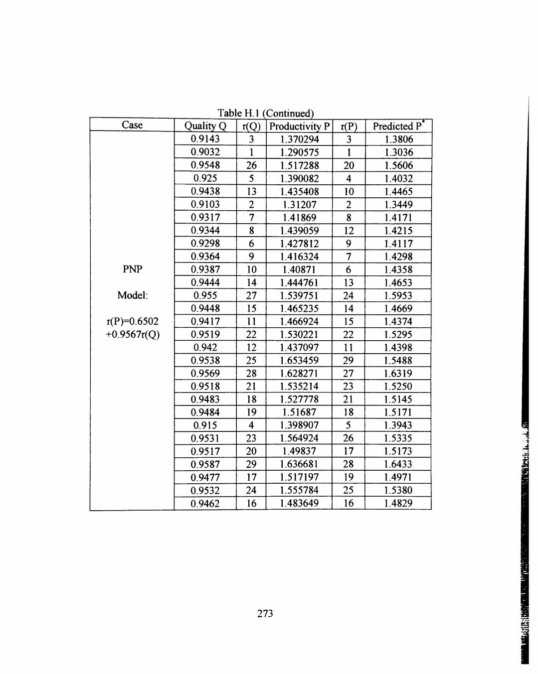
Case
PNP
Model:
r(P)=0.6502 +0.9567r(Q)
Table H. 1 (Continued) Quality Q 0.9143 0.9032
0.9548 0.925 0.9438 0.9103 0.9317 0.9344 0.9298 0.9364 0.9387 0.9444 0.955 0.9448 0.9417 0.9519 0.942 0.9538 0.9569 0.9518 0.9483 0.9484 0.915 0.9531 0.9517 0.9587
0.9477
0.9532 0.9462
r(Q) 3
1 26 5
13 2 7 8 6 9 10 14 27 15 11 22 12 25 28 21 18 19 4 23 20 29 17
24 16
Productivity P 1.370294 1.290575 1.517288
1.390082 1.435408 1.31207 1.41869 1.439059 1.427812 1.416324 1.40871 1.444761 1.539751 1.465235 1.466924 1.530221 1.437097 1.653459 1.628271 1.535214 1.527778 1.51687 1.398907 1.564924 1.49837 1.636681 1.517197 1.555784 1.483649
r(P) 3
1 20 4
10 2 8 12 9 7 6 13 24 14 15
22 11 29 27 23 21 18 5 26 17 28 19 25 16
Predicted P' 1.3806 1.3036
1.5606 1.4032 1.4465 1.3449 1.4171 1.4215 1.4117 1.4298 1.4358 1.4653 1.5953 1.4669 1.4374 1.5295 1.4398 1.5488 1.6319 1.5250 1.5145 1.5171 1.3943 1.5335 1.5173 1.6433 1.4971 1.5380 1.4829
.-.•« . . j ;
:^
273 tt3
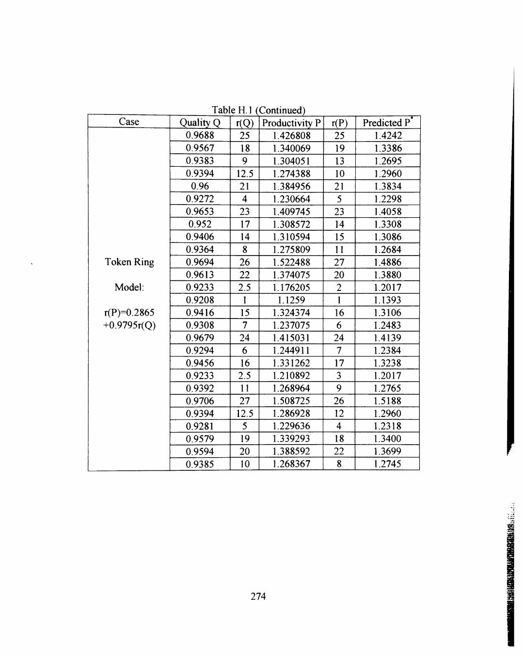
Case
Token Ring
Model:
r(P)==0.2865 +0.9795r(Q)
Table H.l (Continued) Quality Q 0.9688 0.9567 0.9383 0.9394 0.96
0.9272 0.9653 0.952 0.9406 0.9364 0.9694 0.9613 0.9233 0.9208 0.9416 0.9308 0.9679 0.9294 0.9456 0.9233 0.9392 0.9706 0.9394 0.9281 0.9579 0.9594 0.9385
r(Q) 25 18 9
12.5 21 4 23 17 14 8 26 22 2.5 1 15 7 24 6 16 2.5 11 27 12.5 5 19 20 10
Productivity P 1.426808 1.340069
1.304051 1.274388 1.384956 1.230664 1.409745 1.308572 1.310594 1.275809 1.522488 1.374075 1.176205 1.1259 1.324374 1.237075 1.415031 1.244911 1.331262 1.210892 1.268964 1.508725 1.286928 1.229636 1.339293 1.388592 1.268367
r(P) 25 19
13 10
21 5 23 14 15 11 27 20 2 1 16 6 24 7 17 3 9 26 12 4 18 22 8
Predicted P' 1.4242 1.3386
1.2695 1.2960 1.3834 1.2298 1.4058 1.3308 1.3086 1.2684 1.4886 1.3880 1.2017 1.1393 1.3106 1.2483 1.4139 1.2384 1.3238 1.2017 1.2765 1.5188 1.2960 1.2318 1.3400 1.3699 1.2745
274