A subdivision-based implementation of the hierarchical b-spline finite element method

P.B. Bornemann, F. Cirak∗

Department of Engineering, University of Cambridge, Trumpington Street, Cambridge CB2 1PZ, U.K.

Abstract

A novel technique is presented to facilitate the implementation of hierarchical b-splines and their interfacing with conventionalfinite element implementations. The discrete interpretation of the two-scale relation, as common in subdivision schemes, is used toestablish algebraic relations between the basis functions and their coefficients on different levels of the hierarchical b-spline basis.The subdivision projection technique introduced allows us first to compute all element matrices and vectors using a fixed numberof same-level basis functions. Their subsequent multiplication with subdivision matrices projects them, during the assembly stage,to the correct levels of the hierarchical b-spline basis. The proposed technique is applied to convergence studies of linear andgeometrically nonlinear problems in one, two and three space dimensions.

Keywords: Finite elements, hierarchical b-splines, subdivision schemes, isogeometric analysis

1. Introduction

In finite element analysis it is essential to adapt the spa-tial resolution and polynomial degree of the basis functions tothe solution field. Often the resolution of the given CAD ge-ometry differs from the spatial resolution requirements of theanalysis model. The analysis mesh needs to be refined at loca-tions where the solution field has high gradients and, by con-trast, the resolution of the geometry model is determined by thesize and location of the smallest geometric features. In order toaid the implementation of adaptive analysis tools it is necessaryto have a unique mapping between the geometry and finite ele-ment models. To this end isogeometric analysis using b-splinesand related basis functions provides a bidirectional mapping be-tween the geometry and analysis models and holds the promiseto provide a comprehensive solution to adaptive analysis [1, 2].

In computer graphics and geometric modelling there area host of techniques available to adapt locally, i.e. refine orcoarsen the spatial resolution of spline surfaces. Most of thesetechniques rely on the refinability property of b-splines accord-ing to which the spatial resolution of a spline surface can be in-creased without altering its geometry. Refinability is crucial toa number of multiresolution editing techniques, such as knot in-sertion [3], subdivision curves and surfaces [4–6], t-splines [7],hierarchical refinement [8] and wavelets [9, 10]. In algebraicterms, refinability enables the presentation of the b-splines de-fined on a coarse knot sequence as a linear combination of b-splines defined on a finer knot sequence. Thus the refinabilityproperty of b-splines is sometimes also referred to as the two-scale relation. In the context of multiresolution mesh editingrefinability is used locally to replace or overlay selected coarse

∗Corresponding authorEmail address: f.cirak@eng.cam.ac.uk (F. Cirak)

b-splines with finer b-splines [8]. The refined b-spline geome-try is able exactly to reproduce the coarse one and beyond thatgeometric details can be added as necessary.

The common adaptive b-spline refinement techniques avail-able in computer graphics and geometric modelling cannot bedirectly employed in adaptive finite element analysis. Amongothers, these techniques usually do not lead to linearly inde-pendent basis functions, which is important for the finite ele-ment formalism. Recently, two b-spline techniques originat-ing in computer graphics, namely t-splines and hierarchical b-splines, have been extended to finite element analysis [11–13].In t-splines local refinement is performed by inserting one ormore knots into an existing tensor product b-spline patch. Thisis followed by a second step in which additional knots are intro-duced so that all b-splines have the complete set of knot inter-vals. Hierarchical b-spline refinement is performed by overlay-ing a coarse tensor product patch with smaller and finer tensorproduct patches. In both refinement approaches certain ruleshave to be followed so that the resulting basis functions arelinearly independent and retain their polynomial reproductionproperties and smoothness. In terms of software implemen-tation these rules lead to conceptually straightforward but in-tricate algorithms. An additional source of complexity is thebasis function focus of b-spline refinement techniques and theelement focus of conventional finite element software.

In this paper we make use of concepts from subdivisionschemes to ease the implementation of hierarchical b-splinesand to simplify their integration with existing finite elementsoftware. As known, subdivision schemes for curves and sur-faces provide an alternative viewpoint to b-splines [5, 6, 14, 15].They create a smooth curve or surface starting from a coarsecontrol mesh by repeated refinement and averaging, which con-verges to a b-spline curve or surface for certain choices of av-eraging weights. In computer graphics applications subdivision

Preprint submitted to Elsevier July 17, 2012

schemes are often used as simple mesh refinement algorithmsfor creating sufficiently fine faceted presentations of smoothsurfaces. As we shall demonstrate, this algorithmic mesh-basedview of b-splines can greatly ease the implementation of hier-archical b-splines. More specifically it makes it straightforwardto establish algebraic relations between the basis functions andtheir coefficients defined on different refinement levels of themesh. For instance, these relations simplify the evaluation ofthe element matrices and vectors which depend on basis func-tions defined over several levels. In the present approach ele-ment matrices and vectors are all evaluated at the finest avail-able level and are subsequently projected to the hierarchical b-spline space during the finite element assembly stage. This isaccomplished by multiplying the element matrices and vectorswith subdivision matrices. Note that the mapping of coefficientsbetween different hierarchical b-spline levels is also relevantduring the adaptive solution of nonlinear and history-dependentproblems.

The outline of this paper is as follows. Section 2 begins witha brief review of univariate and multivariate b-splines and sum-marises their properties relevant for subsequent discussions. InSection 3 the hierarchical b-splines as defined by Kraft [16]are introduced. Subsequently, in Section 4 the hierarchical b-splines are used for finite element discretisation of boundaryvalue problems. The subdivision projection technique is intro-duced as an effective means of dealing with the complexitiesof hierarchical b-splines and for interfacing them with conven-tional finite elements. Adaptive finite element analysis basedon hierarchical b-splines is applied to different linear and geo-metrically nonlinear examples in Section 5.

2. Review of b-splines and subdivision

In following we briefly review the definition of a few im-portant properties of uniform b-splines. For further details onb-splines we refer to standard textbooks, e.g., [3, 17, 18].

2.1. Univariate b-spline basis functions and their refinability

We consider the uniform b-spline basis functions over a pa-rameter space with equidistantly spaced knots ξi = 0, 1, 2, 3, . . ..The corresponding b-spline basis functions Bµi of degree µ aredefined with the recursive averaging formula

B0i (ξ) =

1 if ξi ≤ ξ < ξi+1

0 otherwise

Bµi (ξ) =ξ − ξi

ξi+µ − ξiBµ−1

i (ξ) +ξi+µ+1 − ξ

ξi+µ+1 − ξi+1Bµ−1

i+1 (ξ)

(1)

Without going into detail, a b-spline of degree µ is non-zeroover an interval ξi ≤ ξ < ξi+µ+1. The uniform b-splines ofdegree µ computed with (1) are the shifted (or, translated) in-stances of each other, i.e. Bµi (ξ) = Bµ0(ξ − i). At the top halfof Figure 1 translates of a few quadratic b-splines are shownand the indexing (labelling) scheme implied by (1) is indicated.The index of a b-spline Bµi is the same as the index of the knotlocated at its support’s lower boundary ξi = i. As will become

0 1 2 3 i i+1 i+2 i+3 i+4»

B¹=20 B0,2i B0,2i+1

0 12 1 3

2 2 3 i i+1 i+2 i+3 i+4»

B`=1,¹=20

B1,22i B1,22i+1 B1,22i+2

Figure 1: Quadratic b-splines B`,µi on levels ` = 0 and ` = 1obtained by translation and scaling of Bµ=2

0 .

apparent later, the present labelling scheme allows us to con-sider odd and even degree b-splines within the same algorithmicframework.

In addition to the knot sequence considered so far we intro-duce an `-times bisected knot sequence ξ`i = 0/2`, 1/2`, 2/2`,3/2`, 4/2`, . . . with level ` ≥ 0. This means that the index i ofa particular knot ξ0

i = i on the initial knot sequence with ` = 0becomes index 2`i at level `, that is ξ`2`i = ξ0

i . A scaling relationholds between the basis functions on the initial knot sequencewith ` = 0 and the `-times bisected knot sequence

B`,µi (ξ) = Bµ0(2`ξ − i) (2)

where the factor 2` in the argument scales the support size of abasis function at level ` with respect to the initial support size.

B-spline basis functions are refinable in the sense that theb-splines B`,µi (ξ) on level ` can be represented as a linear com-bination of B`+1,µ

j (ξ) on level ` + 1

B`,µi (ξ) =∑

k

S µi,kB`+1,µ

2i+k (ξ) with S µi,k =

12µ

(µ + 1

k

)(3)

Here, S µi,k is the subdivision matrix and its entries, the subdi-

vision weights, are given in terms of the usual binomial coef-ficients [4, 5, 19]. The subdivision matrix is a banded sparsematrix with identical rows and columns. Its components are in-dependent of the knot index i and the level `, but depend onthe polynomial degree µ of the considered b-spline. The µ + 2b-splines B`+1,µ

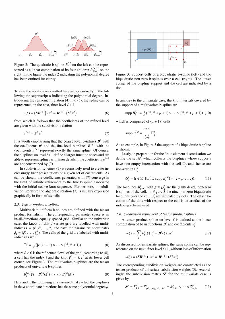
2i+k on the refined knot sequence reproducing theb-spline B`,µi are referred to as the children of B`,µi . See Figure 2for an illustration of the refinement relation in case of quadraticb-splines.

At times it is more convenient to write (3) in matrix notation

B`,µ = SµB`+1,µ (4)

2.2. Subdivision refinement of univariate splinesA spline on level ` is defined as the product of the basis

functions B`i with the coefficients u`i

u(ξ) =∑

i

B`i (ξ) u`i = B`(ξ) · u` (5)

2

»

B`i

»`2i »`i+1 »`i+2 »`i+3»

14 B`+12i

34 B`+12i+1

34 B`+12i+2

14 B`+12i+3

»`+12i »`+12i+2 »`+12i+4 »`+12i+6

Figure 2: The quadratic b-spline B`,2i on the left can be repre-sented as a linear combination of its four children B`+1,2

2i+k on theright. In the figure the index 2 indicating the polynomial degreehas been omitted for clarity.

To ease the notation we omitted here and ocasionally in the fol-lowing the superscript µ indicating the polynomial degree. In-troducing the refinement relation (4) into (5), the spline can berepresented on the next, finer level ` + 1

u(ξ) =(SB`+1

)· u` = B`+1 ·

(S>u`

)(6)

from which it follows that the coefficients of the refined levelare given with the subdivision relation

u`+1 = S>u` (7)

It is worth emphasising that the coarse level b-splines B` withthe coefficients u` and the fine level b-splines B`+1 with thecoefficients u`+1 represent exactly the same spline. Of course,the b-splines on level `+1 define a larger function space and areable to represent splines with finer details if the coefficients u`+1

are not constrained by (7).In subdivision schemes (7) is recursively used to create in-

creasingly finer presentations of a given set of coefficients. Ascan be shown, the coefficients generated with (7) converge inthe limit of infinite refinement to the true b-spline associatedwith the initial coarse knot sequence. Furthermore, in subdi-vision literature the algebraic relation (7) is usually expressedgraphically in form of stencils.

2.3. Tensor product b-splinesMultivariate uniform b-splines are defined with the tensor

product formalism. The corresponding parameter space is anin-all-directions equally spaced grid. Similar to the univariatecase, the knots on this d-variate grid are labelled with multi-indices i = (i1, i2, . . . , id) and have the parametric coordinatesξi = (ξ1

i1 , . . . , ξdid ). The cells of the grid are labelled with multi-

indices as well

`i = 12`([i1, i1 + 1) × · · · × [id, id + 1)

)(8)

where ` ≥ 0 is the refinement level of the grid. According to (8),a cell has the index i and the knot ξ`i = i/2` at its lower cellcorner, see Figure 3. The multivariate b-splines are the tensorproducts of univariate b-splines

B`,µi (ξ) = B`,µi1 (ξ1) × · · · × B`,µid (ξd) (9)

Here and in the following it is assumed that each of the b-splinesin the d coordinate directions has the same polynomial degree µ.

Figure 3: Support cells of a biquadratic b-spline (left) and thebiquadratic non-zero b-splines over a cell (right). The lowercorner of the b-spline support and the cell are indicated by adot.

In analogy to the univariate case, the knot intervals covered bythe support of a multivariate b-spline are

supp B`,µi = 12`([i1, i1 + µ + 1) × · · · × [id, id + µ + 1)

)(10)

which is comprised of (µ + 1)d cells

supp B`,µi =

i+µ+1⋃j=i

`j

As an example, in Figure 3 the support of a biquadratic b-splineis shown.

Lastly, in preparation for the finite element discretisation wedefine the set G`j which collects the b-splines whose supportshave non-empty intersection with the cell `j and, hence arenon-zero in `j,

G`j = i ∈ Zd |`j ⊂ supp B`,µi = j − µ, . . . , j (11)

The b-splines B`g, µ with g ∈ G`j are the (same-level) non-zerob-splines of the cell. In Figure 3 the nine non-zero biquadraticb-splines over the cell `j are indicated by dots. The offset lo-cation of the dots with respect to the cell is an artefact of theindexing scheme used.

2.4. Subdivision refinement of tensor product splinesA tensor product spline on level ` is defined as the linear

combination of basis functions B`i and coefficients u`i

u(ξ) =∑

i

B`i (ξ) u`i = B`(ξ) · u` (12)

As discussed for univariate splines, the same spline can be rep-resented on the next, finer level `+1, without loss of information

u(ξ) =(SB`+1) · u` = B`+1 ·

(S>u`

)The corresponding subdivision weights are constructed as thetensor products of univariate subdivision weights (3). Accord-ingly, the subdivision matrix Sµ for the multivariate case isgiven by

Sµ = S µi,k = S µ

(i1,...,id),(k1,...,kd) = S µ

i1,k1 × · · · × S µ

id ,kd (13)

3

With this subdivision matrix the refinement relation for mul-tivariate b-splines and the subdivision relation for their coeffi-cients can be expressed in the same way as in the univariatecase, see (4) and (7).

3. Hierarchical b-splines (hb-splines)

The hierarchical b-splines first introduced by Forsey et al.[8] allow local refinement of a given coarse b-spline patch byoverlaying it with finer b-spline patches. The basis functions ondifferent levels are simultaneously considered since the motiva-tion for developing hierarchical b-splines was multiresolutionmesh editing. Hence the resulting basis functions are by con-struction non-local and not always linearly independent. An al-ternative definition of hierarchical b-splines provided by Kraft[16] leads to basis functions better suited to finite element ap-plications. More specifically, the basis functions are linearlyindependent and the support size of the basis functions is rela-tively small.

The hierarchical b-splines can be understood as a techniquefor locally enriching the approximation space by replacing se-lected coarse grid b-splines with fine grid b-splines [12, 13, 20].To this end, it is crucial that the basis functions satisfy a refine-ment relationship as introduced in Section 2.4. The change offocus from element refinement (as in conventional finite ele-ments) to basis refinement is crucial to local b-spline refine-ment. Building on the notion of basis refinement and Kraft’soriginal algorithm, we introduce in this section the hb-splineswhich are constructed in three steps, referred to as the refine-ment, compilation and shrinkage. In short, refinement intro-duces new b-splines at a finer level; compilation assures linearindependence by removing basis functions; and shrinkage dis-cards b-splines at the boundaries with a support not intersectingthe effective domain. As will be specified later the effective do-main is the subdomain on which the coarse b-splines on level` = 0 form a partition of unity.

3.1. Hierarchical univariate b-splines

To begin with we consider the local refinement of univari-ate b-splines defined over a one-dimensional domain. The pre-sented approach and definitions closely follow Kraft [16]. Allthe steps are illustrated with the help of a locally refined qua-dratic b-spline example.

Our starting point is a set of b-spline basis functions whosesupport is fully contained in a parameter domainwith equidis-tantly spaced knots. For simplicity it is assumed that is a con-nected domain. These b-splines and the domain represent thecoarse grid to be refined; they are referred to as the 0-th levelb-splines and initial domain.

:= 0 =⋃i∈I0

supp B0i (14)

whereI0 is the index set containing all the considered b-splines.Figure 4 shows a sample initial domain with |I0| = 8 quadraticb-splines over the knot interval 0 = [0, |I0| + µ).

0 1 2 3 4 5 6 7 8 9 10»

B00 B01 B02 B03 B04 B05 B06 B07

0 1 2 3 4 5 6 7 8 9 10

ut0

Figure 4: Initial domain for quadratic b-splines.

Refinement step. The approximation space formed by the b-splines in I0 can be refined by replacing selected b-splines B0

iwith b-splines B1

i . The b-splines B1i on level 1 are defined on a

grid with cells half as large as those on the initial domain 0.In this step we use the refinement relation introduced in Sec-tion 2.1. Specifically, the Kraft algorithm requires that, if a cer-tain b-spline B0

i is to be refined, all its children on level 1 haveto be introduced, as stipulated by the refinement relation (3).The union of the supports of b-splines on level 1 constitutes thedomain

1 =⋃i∈I1

supp B1i (15)

Note that in general 1 need not be a connected domain. How-ever, the subdomain 1 can always, by construction, be fullycovered with the supports of b-splines on level 0, because allthe children of each refined coarse b-spline B0

i are present onlevel 1. This implies for the domain on level 1 that

1 =⋃j∈I1

supp B1j =

⋃j∈M0

supp B`j (16)

whereM0 is the index set containing all the refined b-splines.In the Kraft algorithm the subdomains are not allowed to in-tersect with the boundary of the coarser, enclosing domain, i.e.

∂0 ∩ ∂1 = ∅ (17)

This means that there is always one cell distance between theboundary of the coarse and fine grid.

In practice the refinement step is applied recursively so thatit leads to a sequence of successively refined domains and b-splines. The refinement of a domain at level ` is carried out inthe same way as the refinement of the initial domain at level 0described above. The non-intersection requirement (17) hasnow to be satisfied between domains on two consecutive re-finement levels

∂` ∩ ∂`+1 = ∅ (18)

The recursive application of the refinement step combined withthe non-intersection requirement leads to a sequence of nestedrefined domains

:= 0 ⊃ 1 ⊃ 2 ⊃ . . . ⊃ `max (19)

where `max is the global maximum refinement level or globallevel width reached during the recursive refinement.

4

0 1 2 3 4 5 6 7 8 9 10»

B00 B01 B02 B04 B05 B06 B07

0 1 2 3 4 5 6 7 8 9 10

ut0

0 1 2 3 4 5 6 7 8 9 10»

B16 B17 B

18 B

19

0 1 2 3 4 5 6 7 8 9 10

ut1

Figure 5: First refinement of quadratic b-splines (after compi-lation).

Compilation step. The set of b-splines created in the refine-ment step is, in general, not linearly independent1 and hencenot suitable for finite element purposes. The aim of the compi-lation step is to assemble a linearly independent basis by sys-tematically adding and discarding redundant b-splines.

To this end we first assume that on each domain`, with ` =

0, . . . , `max, all the b-splines with supp B`i ⊂ ` are present.

Subsequently, starting from level 0 and proceeding level-by-level, we discard any coarse b-spline B`i that can be presentedas a linear combination of existing fine b-splines B`+1

i . This isaccomplished by checking wether all the children of the coarseb-spline B`i (as stipulated by the refinement relation) are presenton the next finer level ` + 1. Evidently this is equivalent tochecking that supp B`i ⊂

`+1. The compilation terminateswhen level `max − 1 is reached.

After discarding the redundant b-splines those remaining oneach level are collected into index sets

D` = i ∈ Z | supp B`i ⊆ ` and supp B`i *

`+1 (20)

The union of the b-splines in all index sets D` establish thehierarchical b-spline basis

Bhb() := spanB`k | 0 ≤ ` ≤ `max and k ∈ D` (21)

As proven by Kraft [16], the hierarchical b-spline basis Bhb islinearly independent on the domain . In this basis the sum ofthe b-splines in certain cells can be different from one. How-ever, the basis is able to reproduce, except close to the bound-aries of the initial domain 0, polynomials up to the b-splinedegree.

Illustrative example. Continuing with the quadratic b-spline ex-ample shown in Figure 4, we describe step-by-step its refine-ment with the technique described above.

Firstly, we refine a single b-spline B03. In the refinement

step, its four children on level 1, namely B16, B1

7, B18 and B1

9, areintroduced. The union of their supports is the subdomain 1 =

[3, 6). Recall, a quadratic b-spline has four children due to therefinement relation introduced in Section 2.1 (c.f. also Fig. 2).The result of the refinement step is shown in Figure 5. In

1A set of functions B`i (ξ) | i ∈ D`, ` ≥ 0 is linearly independent for all ξ ∈⋃i∈D` ,`≥0 supp B`i if the equation 0 =

∑i∈D` ,`≥0 u`i B`i (ξ) has only the (trivial)

solution u`i = 0 for all i ∈ D`, ` ≥ 0.

0 1 2 3 4 5 6 7 8 9 10»

B00 B01 B02 B07

0 1 2 3 4 5 6 7 8 9 10

ut0

0 1 2 3 4 5 6 7 8 9 10»

B16 B17 B

18 B

19B

110B

111B

112B

113B

114B

115

0 1 2 3 4 5 6 7 8 9 10

ut1

Figure 6: Second refinement of quadratic b-splines (after com-pilation).

0 1 2 3 4 5 6 7 8 9 10»

B00 B01 B02 B07

0 1 2 3 4 5 6 7 8 9 10

ut0

0 1 2 3 4 5 6 7 8 9 10»

B16 B18 B19B

110B

111B

112B

113B

114B

115

0 1 2 3 4 5 6 7 8 9 10

ut1

0 1 2 3 4 5 6 7 8 9 10»

B214 B217

0 1 2 3 4 5 6 7 8 9 10

ut2

Figure 7: Third refinement of quadratic b-splines (after compi-lation).

the compilation step only the b-spline B03 is discarded because

supp B03 ⊂

1. The other b-splines on level 0 have to remainas they cannot be presented as a linear combination of the b-splines present on level 1. The index sets of the active b-splineson the two levels areD0 = 0, 1, 2, 4, . . . , 7 andD1 = 6, . . . , 9.

Next, in addition to B03 the b-spline B0

6 is also refined. Inthe refinement step we introduce the four children B1

12, B113, B1

14and B1

15 of B06, see Figure 6. The union of all level 1 b-spline

supports now becomes 1 = [3, 9). In the compilation stepwe at first assume that all b-splines on 0 and 1 are present.Thus the set D1 = 6, . . . , 15 contains 10 b-splines, c.f. Fig-ure 6, and not just the eight children introduced in the refine-ment step. After compilation the set of remaining active indicesfor the zero level isD0 = 0, 1, 2, 7. Note that in addition to B0

3and B0

6 also B04 and B0

5 are discarded because supp B04 ⊂

1 andsupp B0

5 ⊂ 1.

Finally, we refine B17 on level 1. In the refinement step its

four children B214, B2

15, B216 and B2

17 are introduced, see Figure 7.After the compilation we obtain the set of active indices D0 =

0, 1, 2, 7,D1 = 6, 8, . . . , 15 andD2 = 14, . . . , 17.

3.2. Hierarchical tensor product b-splines

It is straightforward to generalise the univariate hierarchicalb-splines to the tensor product case. To this end it is helpfulto remember that the key idea in hierarchical b-spline refine-ment is the replacement of coarse grid b-splines with fine gridb-splines. Starting from this premise, tensor product b-splinescan be locally refined by following the algorithm introduced inSection 3.1.

5

Figure 8: Nested domains over three refinement levels withquadratic hb-splines.

Evidently, in generalising the univariate refinement algo-rithm, we have to take into account the change of dimension ofthe support and the number of children. As introduced in Sec-tion 2.3, the number of children of a d-variate b-spline B`i (ξ) is(µ + 2)d, where µ is its polynomial degree, and supp B`i (ξ) is ad-dimensional domain. Recall that the index i is a multi-indexi = (i1, i2, . . . , id). In the multivariate case the definition of thesubdomains (16) becomes

` =⋃i∈I`

supp B`i (22)

where I` is the index set of the b-splines on level `. As pre-viously stated, for hierarchical refinement these domains haveto be non-intersecting and nested, c.f. (18) and (19), and seeFigure 8. According to (20) the index set of active b-splines oneach level is

D` = i ∈ Zd | supp B`i ⊆ ` and supp B`i *

`+1 (23)

As in the univariate case, the union of active b-splines over alllevels establishes the linear hierarchical tensor product b-splinebasis

Bhb() := spanB`k | 0 ≤ ` < `max and k ∈ D` (24)

Illustrative example. As a continuation of the univariate exam-ple in the foregoing section, a two-dimensional example is con-sidered to highlight the refinement and compilation steps in themulti-variate case, see Figure 9. In this and subsequent figureseach b-spline is indicated by a dot at the lower corner of itssupport.

Firstly, we refine the b-spline B0(3,1), which corresponds to

the missing dot on level 0 in Figure 9. Its support, consisting of3×3 cells, is the highlighted subdomain in0. In the refinementstep the 16 children of B0

(3,1) on level 1 are introduced. Theunion of their supports is1 = [3, 6)×[1, 4). In the compilationstep only the b-spline B0

(3,1) is discarded because supp B0(3,1) ⊆

1. The index set of the active b-splines on level 1 is D1 =

[6, . . . , 9] × [2, . . . , 5].Next, in addition to B0

(3,1) we also refine B0(6,1). The supports

of both b-splines form the connected subdomain 1 = [3, 9) ×

Figure 9: First refinement of quadratic hb-splines (after compi-lation).

Figure 10: Second refinement of quadratic hb-splines (aftercompilation).

[1, 4), c.f. Figure 10. In the compilation step we first assumethat all b-splines on 0 and 1 are present. This means theset D1 comprises in addition to the children of B0

(3,1) and B0(6,1)

the b-splines with the indices k ∈ [10, 11] × [2, . . . , 5]. In thecompilation step, from the set D0 the b-splines B0

(4,1) and B0(5,1)

are removed because their supports are a subset of 1. Theresult after the compilation step is shown in Figure 10.

3.3. Hierarchical tensor product b-splines on effective domain

The introduced hb-spline basis is incomplete in cells closeto the initial domain boundary ∂0. Its polynomial reproduc-tion properties are compromised because in boundary cells someof the b-splines are missing. As can be deduced from the uni-variate case, see Figure 4, for b-splines of degree µ only cellsthat are µ cells away from the domain boundary have the fullset of non-zero b-splines. We therefore introduce the notion ofan effective domain := 0, which is comprised of cells thathave the complete set of non-zero b-splines, see Figure 11. Thecells between the effective and initial domains may be regardedas guard or ghost cells.

The effective domain can be determined by counting the in-tersecting b-splines of the cells on the initial level. If the num-ber of b-splines in

P0j = i ∈ I0 |0

j ⊂ supp B0i

on level 0 is equal to (µ+ 1)d, then a complete basis is availableon cell0

j . The union of all cells with complete basis forms theeffective domain

=⋃j∈J0

0j with J0 = j ∈ Zd | |P0

j | = (µ + 1)d

6

Figure 11: Initial and effective domains in case of quadratic b-splines (µ = 2). The effective domain is the union of the blueshaded cells.

In [16] Kraft proved the linear independence of the hb-basison the domain 0. This property is not immediately guaran-teed on the effective domain . However, Kraft’s proof canbe adapted to the effective domain if the index set of active b-splines D`, see (23), is modified to incorporate the effectivedomain, i.e.

D` = i ∈ Zd |(supp B`i ∩) ⊆ ` and

(supp B`i ∩) * `+1 and

(supp B`i ∩) , ∅

(25)

The three conditions in the index set D` reflect what we re-ferred to as compilation, refinement and shrinkage of b-splinesin the refinement algorithm, see also Appendix A. The threeconditions are complemented with the nestedness property ofthe subdomains, i.e. ` ⊃ `+1, see also (19).

The hierarchical tensor product b-splines on the effectivedomain form the space

Bhb() := spanB`k | 0 ≤ ` ≤ `max and k ∈ D`

which will be used in Section 4 to discretise partial differentialequations with the finite element method.

3.4. Subdivision refinement of hierarchical b-splines

The subdivision refinement of hb-spline interpolants is for-mally identical with the subdivision refinement of b-spline in-terpolants introduced in Sections 2.2 and 2.3. For instance, aspline given on level 0

u(ξ) =∑i∈I0

B0i (ξ) u0

i = B0(ξ) · u0 (26)

can also be interpolated with hb-splines from the space Bhb(),that is

u(ξ) =∑`

∑k∈D`

B`,µk (ξ) u`k =∑`

B`hb(ξ) · u`hb (27)

where the vectors B`hb and u`hb contain the active b-splines and

their coefficients on level `, respectively. Equations (26) and(27) represent the same spline u(ξ) only when the coefficientsu`hb are determined with a refinement relation.

The coefficients u`hb are computed using the subdivision re-finement relation (7) selectively applied to the coefficients ofinactive b-splines. We rewrite (26) as follows

u(ξ) = B0hb(ξ) · u0

hb +∑

j∈I0\D0

B0j (ξ) u0

j (28)

with the second term containing the inactive b-splines on level 0.The coefficients of the inactive b-splines at level 0 are trans-ferred to the b-splines on hierarchy level 1 using subdivision,i.e.

u1j =

∑i∈I0\D0

S µi, j−2i u0

i (29)

The coefficients u1j comprise the coefficients of inactive and ac-

tive hb-splines on level 1. After extracting the coefficients u1hb

of the active b-splines B1hb on level 1, the spline (26) can be

rewritten as

u(ξ) = B0hb(ξ) · u0

hb + B1hb(ξ) · u1

hb +∑

j∈I1\D1

B1j (ξ) u1

j (30)

The last term now holds the inactive b-splines on level 1 whichare next to be replaced with hb-splines on higher levels. Thecorresponding coefficients can be recursively determined withthe selective subdivision (29). This recursive subdivision proce-dure is repeated until all coefficients u`hb in (27) are determined.

The hb-spline basis of Bhb() spans a larger space than thatof the b-splines on level 0. If the selective subdivision relation,i.e. (29) and similarly for higher levels, is not required to hold,geometries can have more detail when interpolating with hb-splines from Bhb().

As an example, in Figure 12 the interpolation of a surfacewith cubic tensor product b-splines and randomly refined hb-splines is shown. The b-spline coefficients in this example arecoordinate vectors in three dimensions. The grid lines on bothspline surfaces are the projections of the tensor product gridin the two-dimensional parameter space. As can be visuallyconfirmed, the surfaces in Figures 12a and 12b are identical.This has been achieved by determining the coefficients of thehb-spline interpolation with the subdivision relation (29).

(a) Initial representation. (b) Locally refined representation.

Figure 12: Same surface represented by two distinct cubic hb-spline bases.

7

4. Finite element discretisation of boundary value problemswith hb-splines

The hb-splines provide a linearly independent, locally re-finable basis with the smoothness and polynomial reproductionproperties of b-splines. Thus they are ideal for adaptive dis-cretisation of boundary value problems with the finite elementmethod. See [12, 13, 19, 20] for finite element related discreti-sation techniques with hb-splines. As discussed in Section 3,hb-splines are inherently basis function centric. At first sightthis appears to be at odds with the element focus of traditionalfinite elements. In this section we introduce the subdivisionprojection technique which provides an elegant means to recon-ciling the two differing viewpoints and to interface traditionalfinite element implementations with hb-splines.

4.1. Governing equations and finite element discretisation

We consider the Poisson equation as a representative second-order boundary value problem. The Poisson equation on thephysical domain Ω is given by

−∇ · ∇u = f in Ω

u = u on ΓD

n · ∇u = g on ΓN

(31)

where u is the prescribed solution field on the Dirichlet bound-ary ΓD and g is the prescribed flux on the Neumann boundarywith the outward normal n. The weak formulation of the Pois-son equation can be stated according to Nitsche [21] as: Findu ∈ H1(Ω) such that

a(u, v)︷ ︸︸ ︷∫Ω

∇u · ∇v dΩ =

b(v)︷ ︸︸ ︷∫Ω

f v dΩ +

∫ΓN

g v dΓ−

γp(u, v)︷ ︸︸ ︷γ

∫ΓD

(u − u) v dΓ

+

∫ΓD

((u − u) n · ∇v + (n · ∇u) v

)dΓ︸ ︷︷ ︸

l(u, v)(32)

for all v ∈ H1(Ω). Herein, γ is a parameter which has to besuitably chosen, see [22, 23]. Our decision to weakly enforcethe Dirichlet boundary conditions is motivated by the observa-tion that b-splines are non-interpolating on the boundaries. Al-ternative approaches for weakly enforcing Dirichlet boundaryconditions include i-splines [24] and Lagrange multipliers [25].

The trial and test functions are discretised with hb-splinesuh, vh ∈ Bhb(Ω) ⊂ H1(Ω), i.e.

uh(ξ) =∑`

B`hb(ξ) · u`hb

vh(ξ) =∑`

B`hb(ξ) · v`hb

(33)

Here the summations are over the levels of the hb-spline basis.

By invoking the isoparametric formalism the physical do-main Ω is expressed as the projection of the effective parameterdomain into the physical space.

xh(ξ) =∑`

B`hb(ξ) · x`hb (34)

In practice only the coordinates of the control points x0 on theinitial coarse grid are given. The subdivision technique intro-duced in Section 3.4 is used to generate the coefficients x`hb forhigher levels such that they exactly replicate the original geom-etry described by the coefficients x0.

Introducing the interpolation equations (33) and (34) intothe generalised weak form (32) yields a linear system of equa-tions with the unknowns u`. For instance, the bilinear forma(u, v) in (32) becomes after discretisation

a(uh, vh) =∑

m

∑`

vmhb>

∫Ω

∇Bmhb ∇B`

hb>

dΩ u`hb = v>Au (35)

in which the unknowns and the integral are assembled into thevector u and matrix A, respectively. In (35) the two summationsare over the levels of the hb-spline basis. Although vm

hb and u`hbare by definition level-specific, the final vectors u and v containall the coefficients in the hb-spline space. The discretisation ofthe other integrals in the generalised weak form (32) proceedsalong the lines of the discretisation of the bilinear form.

4.1.1. Evaluation of the discretised weak formThe discretised integrals resulting from the weak form (32),

like the bilinear form (35), are to be integrated numerically.As usual the integration is accomplished by generating a non-overlapping tiling of the parameter domain and thus the physi-cal domain. A canonical tiling of the parameter domain is givenby the cells of the tensor product grid. As discussed in Sec-tion 3.2, hb-splines have a hierarchy of nested tensor productgrids so that the generation of a non-overlapping tiling requirescare. We shall refer to the non-overlapping tiles as integrationcells or elements, although they are not strictly elements in thetraditional finite element sense.

Before specifying a tiling of the parameter domain, we de-fine the scalar variable level width

Λ(ξ) = max`` ≥ 0 | ξ ∈ supp B`i , i ∈ D` (36)

which is equal to the local maximum of b-spline refinementlevel ` present at the coordinate ξ. As defined in (25), the setD`

refers to the index set of active b-splines on level `. The levelwidth Λ(ξ) is a piecewise constant scalar function due to thenestedness of the subdomains in hb-spline refinement.

With the definition of Λ(ξ) to hand, the integration cells aredefined as the union of the cells which are on the level Λ(ξ);see also the illustrative example below. Formally, the index setof the integration cells can be identified with

T ` = i ∈ Zd |`i ⊂ and Λ(`i ) = ` (37)

8

0 1 2 3 4 5 6 7 8 9 10

¤

01

21

0 level width

0 1 2 3 4 5 6 7 8 9 10

¤

01

21

0

»

ut0

ut1

ut2

level width

nested

domains

a

ut: effective

domain

uti¤ integration

cells

Figure 13: Nested domains of univariate, quadratic b-spline ex-ample shown in Figure 7 and its effective domain, level widthand integration cells.

This definition contains the additional constraint that only in-dices of cells which lie within the effective domain are con-sidered. The introduced tiling is non-overlapping such that

=⋃j∈J0

0j =

⋃k∈T `

`≥0

`k (38)

In this tiling integration cells are identical with the knot inter-vals of the finest active b-splines. This ensures the numericalintegration can be performed as efficiently as possible.

Illustrative example. We reconsider the univariate quadratic b-spline example presented in Section 3.1 to illustrate the defi-nition of integration cells and the evaluation of b-splines. InFigure 13 the hb-spline basis functions after two refinementand compilation steps are reproduced. In addition, Figure 13contains a plot of the level width Λ(ξ) over the domain. Asmentioned, Λ(ξ) is a piecewise constant function with jumps atknots. Below the plot of Λ(ξ), the integration cells are picturedas an alternating band of black and grey line segments.

Continuing with the illustrative example, we consider nextthe evaluation of hb-splines at the point ξ = a indicated in Fig-ure 13. This point lies in the integration cell2

15 = [3.75, 4) andcan be thought of as a quadrature point within that cell. FromFigure 13 can be seen that four b-splines are non-zero at theevaluation point. Thus the interpolation within the cell 2

15 in-volves four b-splines over three distinct levels. In contrast, theinterpolation within most other cells in this example involvesonly three b-splines over one single level.

4.2. Evaluation of the element integrals with subdivision pro-jection

In hb-spline finite elements the interpolation within someintegration cells may depend on b-splines defined across mul-tiple levels. In addition, the number of degrees of freedom perelement, i.e. integration cell, is not constant across the mesh.It is, however, possible to evaluate the element matrices andvectors using a constant number of b-splines from the finestlevel. The matrices and vectors are subsequently projected to

0 1 2 3 4 5 6 7 8 9 10 »

B02 B16 B214

B215

0 1 2 3 4 5 6 7 8 9 10

ut0

3 4 5»

B213 B214

B215

3 4 5

ut152

Figure 14: Representation of hb-splines on integration cell inunivariate example with quadratic b-splines, Figure 7.

the correct levels using subdivision weights. We refer to thisprojection operation as subdivision projection. This new tech-nique facilitates the interfacing of hb-splines with conventionalfinite element implementations which rely on a constant num-ber of shape functions. To this purpose a possible alternativeapproach would be to adapt the Bezier extraction technique pro-posed in [26, 27] to hb-splines.

4.2.1. Basic idea and approachAs discussed throughout the paper, using the refinement re-

lation (4) a b-spline can be expressed as a linear combinationof b-splines on the next finer level. Consequently, when therefinement relation is recursively applied, a b-spline can be ex-pressed as a linear combination of b-splines at any finer level.This observation is used to express all non-zero b-splines withinan integration cell using b-splines from one single level. As aresult, during numerical integration all element integrals willdepend on a fixed number of functions. The subdivision pro-jection weights are subsequently used to map the fixed size el-ement vectors and matrices into the hierarchic approximationspace.

Revisiting the univariate example in Figure 13, the sam-ple evaluation point a = 3.875 lies in integration cell 2

15 =

[3.75, 4). The upper half of Figure 14 shows all active hb-splines in 2

15, namely B02, B1

6, B214 and B2

15. The bottom halfof Figure 14 shows the three same-level non-zero b-splines B2

13,B2

14 and B215 of the integration cell 2

15. Our aim is to representeach non-zero hb-spline over 2

15 as a linear combination of itsthree same-level non-zero b-splines. To begin with, we writefor the same-level non-zero b-splines B2

14 and B215 the identities

B214(ξ) =

[B2

13 B214 B2

15

]·[0 1 0

]︸ ︷︷ ︸t2,214

B215(ξ) =

[B2

13 B214 B2

15

]·[0 0 1

]︸ ︷︷ ︸t2,215

The lower level hb-splines B02 and B1

6 can also be representedusing the three same-level non-zero b-splines of 2

15. Consid-ering the two-scale relation for quadratic hb-splines (Figure 2),

9

the b-spline B16 on level one can be expressed with

B16(ξ) =

[B2

13 B214 B2

15

]·[

34

34

14

]︸ ︷︷ ︸t1,26

Similarly, the weights for the b-spline B02 on level zero can be

found by recursively considering the two-scale relation

B02(ξ) =

[B2

13 B214 B2

15

]·[

34

58

38

]︸ ︷︷ ︸t0,22

The introduced subdivision projection vectors t`,2i for the sam-ple integration cell 2

15, allow us to represent the b-splines oncoarser levels with the same-level non-zero b-splines of the in-tegration cell.

In terms of interpolation of a spline curve u(ξ), the subdi-vision projection has the following consequences. The splinesegment over the integration cell 2

15 uses the coefficients u`i ,i.e.

u∣∣∣2

15= B0

2 u02 + B1

6 u16 + B2

14 u214 + B2

15 u215

This spline curve can also be equally written with

u∣∣∣2

15=

[B2

13 B214 B2

15

]·(t0,22 u0

2 + t1,26 u1

6 + t2,214 u2

14 + t2,215 u2

15

)using the same-level non-zero b-splines of the integration cell2

15 and the subdivision projection vectors t`,2i .

4.2.2. Subdivision projectionIn this section we formalise the subdivision projection tech-

nique and elaborate on the efficient computation of the subdivi-sion projection vectors introduced in the foregoing section. Ashighlighted in the preceding section, the non-zero hb-splinesB`i ∈ Bhb over an integration cell Λ

k can be expressed as alinear combination of same-level non-zero b-splines BΛ

B`i = BΛ · t`,Λi (39)

where the vector t`,Λi is associated with the specific b-spline B`i .For the following it is important that BΛ and Λ

k have the samelevel Λ. Moreover, recall that always ` ≤ Λ so that the projec-tion vectors t`,Λi are always well defined.

A computationally convenient approach to determining theprojection vectors is the subdivision refinement algorithm in-troduced in Sections 2.4 and 3.4. To this end, consider the in-terpolation of a spline with B`i ∈ Bhb and the finer b-splines BΛ,i.e.

u(ξ) =∑

i

B`i (ξ) u`i =∑

j

BΛj (ξ) uΛ

j = BΛ(ξ) · uΛ (40)

and restricted to the spline segment over the cell Λk only the

b-splines that are non-zero on the cell are needed

u∣∣∣Λ

k=

∑j∈GΛ

k

BΛj (ξ) uΛ

j = BΛk (ξ) · uΛ (41)

In line with the standard subdivision approach, introducing (39)in to (40) yields a relation for the coefficients of the spline onthe two distinct levels

uΛ =∑

i

t`,Λi u`i (42)

The coefficients of the finer level Λ are a linear combinationof the coefficients of the coarser level `. When the differencebetween the levels ` and Λ is one, the projection vector t`,Λiis a row of the previously introduced subdivision matrix (3).However, when the difference between ` and Λ is more thanone, t`,Λi represents the result of several subdivision steps.

As proposed in [14], the components of the projection vec-tor t`,Λi can be conveniently determined with the aid of the sub-division algorithm. It is worth repeating that t`,Λi correspondsto a specific control point i at the level `. Hence, in order todetermine t`,Λi with the subdivision algorithm we can assign avalue 1 to the control point i at the level ` and values 0 to allothers. After applying the subdivision refinement algorithm thecoefficients of t`,Λi can be collected from the refined mesh.

As an example, in Figure 15 the computation of the projec-tion vectors using subdivision is illustrated. Imagine the high-lighted cell 2

k in Figure 15b is an integration cell and the b-spline B0

i of level 0 is an active hb-spline. The b-spline B0i is

to be expressed as a linear combination of b-splines B2i on the

same level as the integration cell. The series of three figures inthe bottom half of Figure 15 show how the weights t0,2

i are de-termined using subdivision. In Figure 15b a value 1 is assignedto the control point i and values 0 to all other control points.The coefficients after one and two subdivision refinement stepsare shown in Figures 15c and 15d. The values depicted in Fig-ure 15d are the components of the vector t0,2

i .For subsequent derivations it is convenient to introduce a

picking matrix G`k which extracts all non-zero hb-splines B`i (ξ)

in Bhb over an integration cellΛk . The integration-cell-specific

matrix G`k picks from each level ` the hb-splines which are

non-zero over the cell Λk . Thus the non-zero b-splines of the

cell Λk are the b-splines G`

kB`hb over multiple levels. With this

definition to hand we can formally write for the projection rela-tion (39)

G`kB`

hb(ξ) = T`,Λk BΛ

k (ξ) in ξ ∈ Λk (43)

Here the new matrix T`,Λk is a collection of projection vectors

t`,Λi associated to the non-zero hb-splines over the integrationcell.

Application of subdivision projection to discretisation. We nowproceed to the evaluation of the bilinear and linear forms ap-pearing in the hb-spline discretized weak form (32). Firstly,with the introduced tiling of the problem domain in Section 4.1.1,the domain integrals in the weak form can be determined bysummation of element integrals. After the domain integrals aresplit into element contributions, for example, the discretized bi-linear form (35) reads

a(uh, vh) =∑

m

∑`

vmhb>

∑k

∫ω

∇Bmhb ∇B`

hb>

dωΛk

u`hb (44)

10

(a) Supporting cells ofb-spline B0

i and integra-tion cell2

k on two levelshigher.

(b) Weights on level 0. (c) Weights on level 1. (d) Weights on level 2.

Figure 15: Determining the subdivision projection weights t0,2i

for the quadratic b-spline B0i on the integration cell 2

k to rep-resent B0

i with the same-level non-zero b-splines B2k of the in-

tegration cell.

The element integrals over ωΛk can be transformed into inte-

grals over integration cells Λk in the parametric domain by

invoking the isoparametric mapping. In general only few b-splines B`i ∈ Bhb are non-zero over an element. As introducedpreviously, the non-zero hb-splines over an element ωΛ

k are de-noted with G`

kB`hb, where G`

k is a matrix to pick the relevanthb-splines from level `. Thus we can equally write for (44)

a(uh, vh) =∑

m

∑`

vmhb>

∑k

∫ω

Gmk∇Bm

hb ∇B`hb>G`

k>

dωΛk

u`hb

(45)

The number of non-zero hb-splines over an element ωΛk is not

constant. Therefore we introduce next the subdivision projec-tion (43) into (45) so that the element integrals depend on afixed number of b-splines.

a(uh, vh) =∑

m

∑`

vmhb>

∑k

Tm,Λk

∫ω

∇BΛk ∇BΛ

k>

dωΛk T`,Λ

k>

u`hb

(46)

The element integrals now depend on a fixed number of b-splines all from the same level as the integration cell. As aresult element matrices can be evaluated without considerationof the hierarchic nature of the hb-spline basis. It is equally pos-sible to obtain the element matrices from a conventional finiteelement implementation that uses b-splines as shape functions.The multiplication of the element matrices so obtained withthe T`,Λ

k projects them to the hb-spline space. Importantly, ina finite element framework the multiplication with T`,Λ

k can bedeferred until the assembly stage of the global system matrix.

-1

0

1

0 e- e+ 1

c- b c+

u

x

Figure 16: Solution of the one-dimensional Poisson problem.

Although, we focused in this section on the element matrices,the derivations also apply to element vectors.

Note that it is possible to express the b-splines appearingin (46) as the multiplication of Lagrange basis functions withan additional projection matrix. Expressing (46) with Lagrangebasis functions would enable us immediately to port existingfinite element implementations into the hb-spline finite elementframework.

5. Examples

In this section the optimal convergence and the robustnessof the presented hb-spline finite element method is establishedusing standard linear elasticity benchmark examples. Conver-gence results for uniform and adaptive refinement are given. Inaddition, a geometrically nonlinear elasticity problem is anal-ysed to demonstrate the method’s applicability to nonlinear prob-lems. In all examples the element integrals have been evaluatedusing full Gauss integration. There are more efficient integra-tion schemes for b-splines which we could alternatively haveused [28]. As introduced in Section 4.2.2, the element matri-ces and vectors are first computed on common finite elementswhich all have the same number of shape functions. They aresubsequently assembled with subdivision projection into globalmatrices and vectors. As anticipated, in all numerical examplesthe presented refinement algorithms yield a linearly indepen-dent hb-spline basis.

5.1. One-dimensional Poisson problem

As an introductory example we consider the one-dimen-sional Poisson problem d2u/ dx2 + f = 0 on the domain Ω =

(0, 1). The right hand side f is chosen so that the solution isequal to

u(x) = sin(

1a2(x − b)2 + 2/(5π)

)with a = 10, b = 1/2

(47)

This solution is plotted in Figure 16. It oscillates close to thedomain centre x = b = 1/2 with maxima c∓ = b ∓ 2

√10

a5√π

and

minima e∓ = b ∓ 2a√

15π. It tends, however, to level off towards

the both ends of the domain. The hb-splines are ideally suitedto capture the local oscillations in the solution.

11

10-11

10-10

10-9

10-8

10-7

10-6

10-5

10-4

10-3

10-2

102 103 104

ku-uhk 0

N

3

4

uniformadaptive

10-11

10-10

10-9

10-8

10-7

10-6

10-5

10-4

10-3

10-2

102 103 104

ku-uhk 0

N

3

4

quadratic (¹=2)cubic (¹=3)

Figure 17: Convergence FE sinusoidal solution.

0

1

2

3

4

5

0 c- e- b e+ c+ 1

¤

x

Figure 18: Local level width after 40 adaptive steps for cubicb-spline case.

For this example, despite the solution u(x) being oscillatory,optimal convergence rates can be achieved for uniform refine-ment. The relevant standard finite element error estimate reads

‖u − uh‖0 ≤C

Nµ+1 (48)

where uh is the finite element solution, C is a constant, N is thetotal number of degrees of freedom, µ the polynomial degreeof the b-splines and ‖ · ‖0 is the standard L2-norm. As shownin Figure 17, uniform refinement essentially leads to the pre-dicted convergence rates for quadratic and cubic b-splines. Alsoshown in Figure 17 are the convergence of adaptively refinedhb-splines. As implemented here, adaptive refinement is an it-erative procedure and at each refinement step the hb-splines ofthe element with maximum error are refined. In Figure 17 onlyevery 10th refinement step is indicated with ‘N’ or ‘’, respec-tively. As expected, adaptive refinement yields the maximumconvergence rate as the uniform refinement. However, the con-stant C in estimate (48) is significantly lower in case of adaptiverefinement. As a result, the L2-error for adaptive refinement isin comparison with uniform refinement by orders of magnitudesmaller for a given number of N b-splines.

Overall 40 adaptive refinement steps have been performedleading to about 2000 active b-splines. As indicated in Fig-ure 18 the maximum refinement occurs close to the centre ofthe domain. The maximum generational difference between thecoarse and fine level b-splines is 5. Hence, the smallest refinedcells are 25 times smaller than the original coarse cells.

Figure 19: Problem description of bar with variable cross-section.

0

0.5

1

1.5

0 0.25 0.5 0.75 1

u

x

µ=0

µ=0.25

µ=0.5

µ=0.75

Figure 20: Bar with variable cross-section. Displacements forfour singularity strengths θ and spring constant c = 0.5.

5.2. Bar with geometric singularity

An elastic bar with variable cross-section A(x) = xθ, with0 < θ < 1, has a singular solution and as such it is useful tostudy the performance of refinement techniques [29, 30]. Theboundary value problem for the bar shown in Figure 19 reads

ddx

(EA(x)

dudx

)+ p = 0 in Ω = (0, L)

u(x) = 0 at x = 0

EA(x)dudx

= −cu(x) at x = L

(49)

Its solution in dependence of the free parameter θ is easily de-termined

u(x) = −x2−θ

2 − θ+

E + c2−θ

E + c1−θ

x1−θ

1 − θ(50)

The displacements have a singularity at x = 0 for θ > 0 and thechoice of θ controls the strength of the singularity. For instance,for θ = 1/2 the solution exhibits a certain similarity to a cracktip in a two-dimensional plate. In Figure 20, the solutions u(x)for four representative values of θ are shown.

Due to the singularity at the left boundary the theoreticalconvergence rates for this problem are less than optimal forθ , 0. In Figure 21 the convergence of the displacement er-rors in L2-norm for different polynomial degrees and singular-ity strengths are shown. As can be seen, for uniform refinementthe convergence order for θ = 0.25, θ = 0.5 and θ = 0.75is independent of the polynomial degree of the used b-spline.For θ = 0 the solution (50) is a quadratic polynomial so that theconvergence order for linear b-splines is quadratic (Figure 21a);and the solution can be exactly reproduced by the quadratic andcubic b-splines.

12

10-5

10-4

10-3

10-2

10-1

100

100 101 102 103

ku-uhk 0/kuk 0

N

uniformregressive

10-5

10-4

10-3

10-2

10-1

100

100 101 102 103

ku-uhk 0/kuk 0

N

µ=0 µ=0.25 µ=0.5 µ=0.75

(a) Linear b-splines

10-5

10-4

10-3

10-2

10-1

100

100 101 102 103

ku-uhk 0/kuk 0

N

uniformregressive

10-5

10-4

10-3

10-2

10-1

100

100 101 102 103

ku-uhk 0/kuk 0

N

µ=0.25 µ=0.5 µ=0.75

(b) Quadratic b-splines

10-5

10-4

10-3

10-2

10-1

100

100 101 102 103

ku-uhk 0/kuk 0

N

uniformregressive

10-5

10-4

10-3

10-2

10-1

100

100 101 102 103

ku-uhk 0/kuk 0

N

µ=0.25 µ=0.5 µ=0.75

(c) Cubic b-splines

Figure 21: Bar with variable cross-section. Convergence of therelative displacement error in L2 norm.

Figure 22: Geometry of the L-shaped domain.

By choosing an appropriate non-uniform refinement the de-crease in convergence rates with increasing θ can be mitigated.As depicted in Figure 21 this is demonstrated with the increaseof convergence rates for singularity strength θ = 0.75. Theconvergence curves associated with non-uniform refinement arereferred to as ‘regressive’. In the specific refinement strategyused, we successively refine near x = 0 and near x = 1 therefinement remains constant after the first step.

5.3. L-shaped domainThe Laplace equation on the L-shaped domain Ω = (−1, 1)2\

[0, 1]2 is a widely used benchmark example used for studyingadaptive refinement, Figure 22. We demonstrate with this ex-ample the effectiveness of local hierarchical b-spline refinementin case of a two-dimensional domain with a singularity. Theproblem setup is chosen such that the exact solution is

ur(r, θ) = r2/3 sin(2θ/3 − π/3) for r > 0 and 0 < θ ≤ 2π(51)

We computed this example with quadratic and cubic b-splinesusing uniform and hierarchical refinement. In all the computa-tions the Dirichlet boundary conditions are applied with Nitsche’s

Error H1

0.00

0.0520

0.104

0.156

0.208

(a) Initial.

Error H1

0.00

0.0520

0.104

0.156

0.208

(b) 4th step.

Error H1

0.00

0.0520

0.104

0.156

0.208

(c) 8th step.

Figure 23: L-shaped domain. Evolution of H1-seminorm errorisocontours for adaptive refinement with cubic hb-splines.

10-5

10-4

10-3

10-2

10-1

100

102 103 104 105er

ror

N

uniformadaptive

10-5

10-4

10-3

10-2

10-1

100

102 103 104 105er

ror

N

L2semi H1

(a) Quadratic b-splines.

10-5

10-4

10-3

10-2

10-1

100

102 103 104 105

erro

r

N

uniformadaptive

10-5

10-4

10-3

10-2

10-1

100

102 103 104 105

erro

r

N

L2semi H1

(b) Cubic b-splines.

Figure 24: L-shaped domain. Convergence of the solution er-rors in L2-norm and H1-seminorm.

method and γ = 1010. The parameter γ has been chosen largein order to sidestep the discussion about its optimal value. Apossible estimation procedure for the parameter γ based on lo-cal eigenvalue problems can be found in [22]. The local re-finement is carried out by successive refinement of integrationcells which exhibit the largest error in the H1-seminorm, seeFigure 23. Or more precisely, the b-splines which are non-zero over the integration cells are refined. The error in theH1-seminorm is determined with respect to the known exactsolution (51).

The convergence of the L2-norm and H1-seminorm errorsfor uniform and adaptive refinement are compared in Figure 24.As expected the adaptive refinement strategy places fine hb-splines at the reentrant corner. The integration cells and H1-seminorm errors for the corresponding computations with cubicb-splines are given in Figure 23. The loss of optimal conver-gence rate for the uniform case due to the presence of the reen-trant corner is apparent. The local adaptive refinement is able tomitigate this drop in the convergence order and gives highly ac-curate solutions with significantly less degrees of freedom thanin the uniform case.

5.4. Geometrically nonlinear three-dimensional solidIn this last example we present the discretisation of a geo-

metrically nonlinear problem with hb-splines. The discretisa-tion of nonlinear problems with hb-splines is straightforward ashb-splines are independent of the specific considered boundaryvalue problem. In fact, as discussed in Section 4.2.2, using theproposed subdivision projection technique, existing nonlinearfinite element implementations can readily be interfaced withthe proposed hb-spline framework.

13

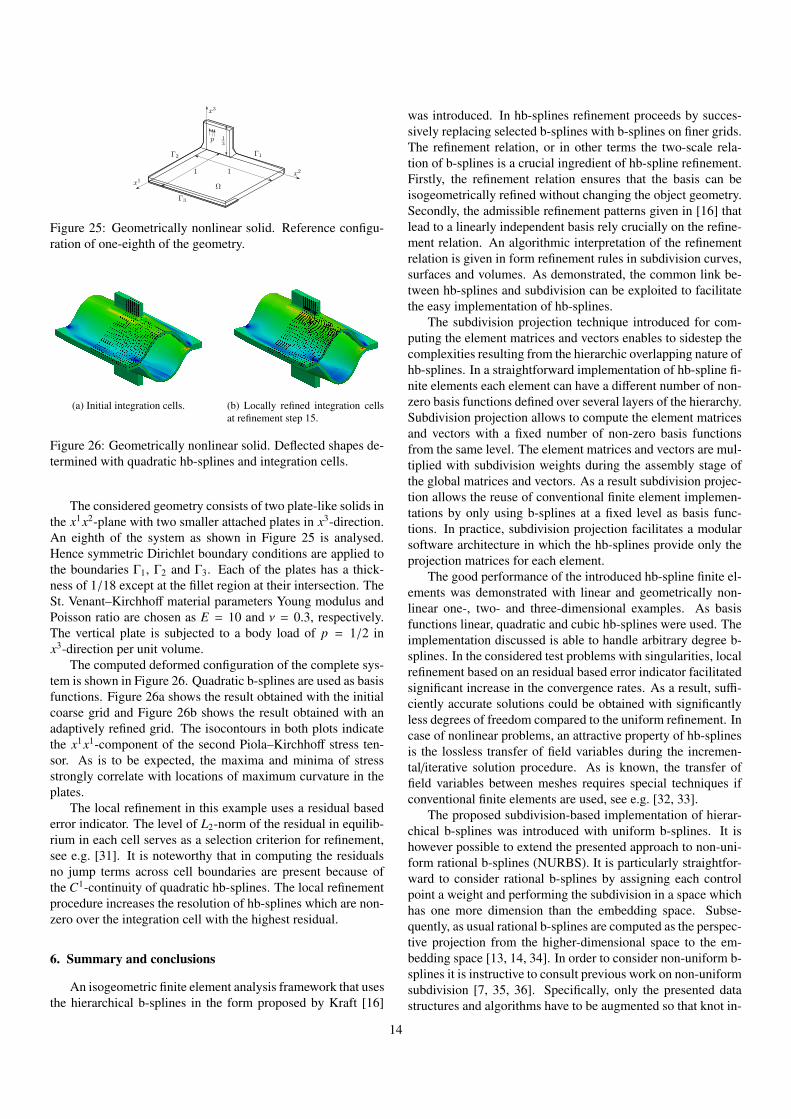
Figure 25: Geometrically nonlinear solid. Reference configu-ration of one-eighth of the geometry.

(a) Initial integration cells. (b) Locally refined integration cellsat refinement step 15.

Figure 26: Geometrically nonlinear solid. Deflected shapes de-termined with quadratic hb-splines and integration cells.

The considered geometry consists of two plate-like solids inthe x1x2-plane with two smaller attached plates in x3-direction.An eighth of the system as shown in Figure 25 is analysed.Hence symmetric Dirichlet boundary conditions are applied tothe boundaries Γ1, Γ2 and Γ3. Each of the plates has a thick-ness of 1/18 except at the fillet region at their intersection. TheSt. Venant–Kirchhoff material parameters Young modulus andPoisson ratio are chosen as E = 10 and ν = 0.3, respectively.The vertical plate is subjected to a body load of p = 1/2 inx3-direction per unit volume.

The computed deformed configuration of the complete sys-tem is shown in Figure 26. Quadratic b-splines are used as basisfunctions. Figure 26a shows the result obtained with the initialcoarse grid and Figure 26b shows the result obtained with anadaptively refined grid. The isocontours in both plots indicatethe x1x1-component of the second Piola–Kirchhoff stress ten-sor. As is to be expected, the maxima and minima of stressstrongly correlate with locations of maximum curvature in theplates.

The local refinement in this example uses a residual basederror indicator. The level of L2-norm of the residual in equilib-rium in each cell serves as a selection criterion for refinement,see e.g. [31]. It is noteworthy that in computing the residualsno jump terms across cell boundaries are present because ofthe C1-continuity of quadratic hb-splines. The local refinementprocedure increases the resolution of hb-splines which are non-zero over the integration cell with the highest residual.

6. Summary and conclusions

An isogeometric finite element analysis framework that usesthe hierarchical b-splines in the form proposed by Kraft [16]

was introduced. In hb-splines refinement proceeds by succes-sively replacing selected b-splines with b-splines on finer grids.The refinement relation, or in other terms the two-scale rela-tion of b-splines is a crucial ingredient of hb-spline refinement.Firstly, the refinement relation ensures that the basis can beisogeometrically refined without changing the object geometry.Secondly, the admissible refinement patterns given in [16] thatlead to a linearly independent basis rely crucially on the refine-ment relation. An algorithmic interpretation of the refinementrelation is given in form refinement rules in subdivision curves,surfaces and volumes. As demonstrated, the common link be-tween hb-splines and subdivision can be exploited to facilitatethe easy implementation of hb-splines.

The subdivision projection technique introduced for com-puting the element matrices and vectors enables to sidestep thecomplexities resulting from the hierarchic overlapping nature ofhb-splines. In a straightforward implementation of hb-spline fi-nite elements each element can have a different number of non-zero basis functions defined over several layers of the hierarchy.Subdivision projection allows to compute the element matricesand vectors with a fixed number of non-zero basis functionsfrom the same level. The element matrices and vectors are mul-tiplied with subdivision weights during the assembly stage ofthe global matrices and vectors. As a result subdivision projec-tion allows the reuse of conventional finite element implemen-tations by only using b-splines at a fixed level as basis func-tions. In practice, subdivision projection facilitates a modularsoftware architecture in which the hb-splines provide only theprojection matrices for each element.

The good performance of the introduced hb-spline finite el-ements was demonstrated with linear and geometrically non-linear one-, two- and three-dimensional examples. As basisfunctions linear, quadratic and cubic hb-splines were used. Theimplementation discussed is able to handle arbitrary degree b-splines. In the considered test problems with singularities, localrefinement based on an residual based error indicator facilitatedsignificant increase in the convergence rates. As a result, suffi-ciently accurate solutions could be obtained with significantlyless degrees of freedom compared to the uniform refinement. Incase of nonlinear problems, an attractive property of hb-splinesis the lossless transfer of field variables during the incremen-tal/iterative solution procedure. As is known, the transfer offield variables between meshes requires special techniques ifconventional finite elements are used, see e.g. [32, 33].

The proposed subdivision-based implementation of hierar-chical b-splines was introduced with uniform b-splines. It ishowever possible to extend the presented approach to non-uni-form rational b-splines (NURBS). It is particularly straightfor-ward to consider rational b-splines by assigning each controlpoint a weight and performing the subdivision in a space whichhas one more dimension than the embedding space. Subse-quently, as usual rational b-splines are computed as the perspec-tive projection from the higher-dimensional space to the em-bedding space [13, 14, 34]. In order to consider non-uniform b-splines it is instructive to consult previous work on non-uniformsubdivision [7, 35, 36]. Specifically, only the presented datastructures and algorithms have to be augmented so that knot in-

14

tervals are stored and refined. In the introduced implementationwe assumed that the knot intervals on each level are constantand are refined by bisection.

A further avenue for future research is the development ofhb-splines for unstructured surface meshes. Grinspun et al. [20]have introduced a basis refinement technique for Loop subdi-vision surfaces similar to hb-splines. Recent results on higher-degree, non-uniform subdivision surfaces, see [36], make it fea-sible to develop NURBS-compatible hb-splines for unstructuredsurface meshes. Different from the surface case, the mathemati-cal theory of subdivision on unstructured volume meshes is stillvery sparse. Therefore, immersed boundary type methods, alsoknown as fictitious domain or embedded domain methods, incombination with hb-splines appear to be promising for prob-lems with arbitrary topology [34].

Appendix A. Data structures and algorithms

In this appendix we discuss the implementation of hb-splinesfocusing on data structures and algorithms. As introduced inSection 3, hb-spline refinement proceeds in three sub-steps re-ferred to as the refinement, compilation and shrinkage steps.

There are two different type of relations in the hb-spline ba-sis which have to be managed. The first is the spatial relationbetween the supports of b-splines on the same level and the sec-ond is the parent-child relation between b-splines on differentrefinement levels. The relation between b-splines on the samelevel is effectively captured by the multi-index labelling of thetensor product grid and b-splines. For encoding the relation be-tween b-splines on different levels a recursive tree data structureis the most straightforward choice. Each node of the hb-splinetree represents a b-spline and stores its multi-index i ∈ Zd, re-finement level ` and an activity tag. The nodes of the tree arelinked according to the refinement relation (3). The set of allactive b-splines D`, or in short D`, is collected by extractingall active b-splines in the complete index set (or tree) I`.

Before introducing the algorithms, we define two auxiliaryindex sets for describing the parent-child relation between b-splines on two consecutive levels.

• The index set of children C`i = k ∈ Zd | supp B`+1k ⊂

supp B`i stores the (µ + 2)d b-splines on the next finerlevel needed to represent B`i .

• The index set of ancestors A`i = k ∈ Zd | supp B`−1

k ⊃

supp B`i contains all b-splines on the coarser level ` − 1which cover completely the support of B`i . Note, |A`

i | isonly constant for even degree splines.

Moreover, we define the following set of update operations mim-icking C-language syntax:

• A∪=B is short forA := A∪B; and

• A\=B is short forA := A \ B.

The in the following listed algorithms cover refinement, un-refinement and methods for integration cells. The refinementalgorithm 1 uses the three steps presented in algorithms 2, 3 and

4. Algorithm 5 shows how by parsing the active hb-splines D`,the integration cells can be collected. Algorithm 6 shows how tocollect all active hb-splines on an integration cell. The unrefine-ment algorithm 7 contains algorithm 8 in which the hb-splinetree Im is reduced in such a way that the targeted b-spline B`iis active again. The coefficients are transferred to the unrefinedhb-splines with a least-squares fit in algorithm 9.

Algorithm 1 RefinementInput: , Im, Dm, (i, `) with i ∈ D`

1: Refine((i, `), Im)2: Compile(Im, Dm)3: Shrink(, Dm)

Output: Im, Dm

Algorithm 2 RefineInput: (i, `), Im

1: // expand indirectly domain at level `+ 1 by adding children of B`i

2: I`+1 ∪=C`i3: // collect domain at level ` + 14: `+1 = ∅5: for each i ∈ I`+1 do6: `+1 ∪= supp B`+1

j7: // complete index set at level ` + 18: for each supp B`+1

i ⊂ `+1 do9: I`+1 ∪=i

Output: Im

Algorithm 3 CompileInput: Im, Dm

1: // construct linearly independent proceeding level-by-level2: for each m = 0, 1, . . . do3: // discard b-splines which are refined4: Dm = ∅5: for each i ∈ Im do6: if Cm

i 1 Im+1 then

7: Dm ∪=iOutput: Dm

15

Algorithm 4 ShrinkInput: , Dm

1: for each m = 0, 1, . . . do2: // discard b-splines which are outside of effective domain3: for each i ∈ Dm do4: if (supp Bm

i ∩) = ∅ then5: Dm \=i

Output: Dm

Algorithm 5 CollectIntegrationCellsInput: T ` = ∅

1: for each ` = 0, 1, . . . do2: // collect domain at level ` + 13: `+1 = ∅4: for each k ∈ D`+1 do5: `+1 ∪= supp B`+1

k6: // identify integration cells on level `7: T ` = ∅8: for each i ∈ D` do9: for each `k ⊂ supp B`i do

10: if `k 1 `+1 then

11: T ` ∪=kOutput: T `

Acknowledgement

The support of the EPSRC through grant # EP/G008531/1is gratefully acknowledged.

References

[1] T. J. R. Hughes, J. A. Cottrell, Y. Bazilevs, Isogeometric analysis: CAD,finite elements, NURBS, exact geometry and mesh refinement, ComputerMethods in Applied Mechanics and Engineering 194 (2005) 4135–4195.

[2] F. Cirak, M. J. Scott, E. K. Antonsson, M. Ortiz, P. Schroder, Integratedmodeling, finite-element analysis, and engineering design for thin-shellstructures using subdivision, Computer-Aided Design 34 (2002) 137–148.

[3] L. Piegl, T. W., The NURBS book, Monographs in visual communication,Springer, 2 edn., 1997.

[4] J. M. Lane, R. F. Riesenfeld, A theoretical development for the computergeneration and display of piecewise polynomial surfaces, IEEE Transac-tions on Pattern Analysis and Machine Intelligence PAMI-2 (1980) 35–46.

[5] D. Zorin, P. Schroder, Subdivision for Modeling and Animation, SIG-GRAPH 2000 Course Notes, 2000.

[6] J. Warren, H. Weimer, Subdivision methods for geometric design: A con-structive approach, Morgan Kaufmann, 2001.

[7] T. W. Sederberg, J. Zheng, A. Bakenov, A. Nasri, T-splines and T-NURCCs, in: SIGGRAPH 2003 Conference Proceedings, San Diego,CA, 2003.

[8] D. R. Forsey, R. H. Bartels, Hierarchical b-spline refinement, ComputerGraphics 22 (1988) 205–212.

[9] S. J. Gortler, M. F. Cohen, Hierarchical and variational geometric model-ing with wavelets, in: Proceedings of the 1995 symposium on interactive3D graphics, 1995.

[10] M. Lounsbery, T. D. DeRose, J. Warren, Multiresolution analysis for sur-faces of arbitrary topological type, ACM Transactions of Graphics 16(1997) 34–73.

[11] Y. Bazilevs, V. M. Calo, J. A. Cottrell, J. A. Evans, T. J. R. Hughes, S. Lip-ton, M. A. Scott, T. W. Sederberg, Isogeometric analysis using T-splines,

Algorithm 6 CollectHierarchicBSplinesOnCellInput: (k, `), Jm = ∅

1: // get shape same-level non-zero b-splines of cell contained in ac-tive hb-splines

2: J ` = G`k ∩D`

3: // find all non-zero hb-splines at coarser levels4: for each m = ` − 1, . . . , 0 do5: for each i ∈ Jm+1 do6: Jm ∪=(Am+1

i ∩Dm)Output: Jm

Algorithm 7 UnrefinementInput: , Im, Dm, (i, `) with i ∈ I` \ D`, um

j

1: Unrefine((i, `), Im)2: Compile(Im, Dm

3: Shrink(, Dm)4: UnrefineCoefficients(, Dm, um

j , Dm, um

j )5: Dm = Dm; um

j = umj

Output: Im, Dm, umj

Computer Methods in Applied Mechanics and Engineering (2010) 229–263.

[12] D. Schillinger, E. Rank, An unfitted hp-adaptive finite element methodbased on hierarchical B-splines for interface problems of complex ge-ometry, Computer Methods in Applied Mechanics and Engineering 200(2011) 3358–3380.

[13] A.-V. Vuong, C. Gianelli, B. Juttler, B. Simeon, A hierarchical approachto adaptive local refinement in isogeometric analysis, Computer Methodsin Applied Mechanics and Engineering 200 (2011) 3554–3567.

[14] F. Cirak, Q. Long, Subdivision shells with exact boundary control andnon-manifold geometry, International Journal for Numerical Methods inEngineering 88 (2011) 897–923.

[15] F. Cirak, M. Ortiz, P. Schroder, Subdivision surfaces: A new paradigmfor thin-shell finite-element analysis, International Journal for NumericalMethods in Engineering 47 (2000) 2039–2072.

[16] R. Kraft, Adaptive and linearly independent multilevel B-splines, in:A. L. Mehaute, C. Rabut, L. L. Schumaker (Eds.), Surface Fitting andMultiresolution Methods, Vanderbilt University Press, 209–218, 1997.

[17] C. de Boor, A practical guide to splines, Springer, 2001.[18] G. Farin, Curves and Surfaces for CAGD, Academic Press, 2002.[19] K. Hollig, Finite Element Methods with B-splines, SIAM Frontiers in

Applied Mathematics, 2003.[20] E. Grinspun, P. Krysl, P. Schroder, CHARMS: a simple framework for

adaptive simulation, in: SIGGRAPH 2002 Conference Proceedings, SanAntonio, TX, 281–290, 2002.

[21] J. Nitsche, Uber ein Variationsverfahren zur Losung von Dirichlet-Problemen bei der Verwendung von Teilraumen, die keinen Randbedin-gungen unterworfen sind, Abhandlungen aus dem Mathematischen Sem-inar der Universitat Hamburg 36 (1971) 9–15.

[22] A. Embar, J. Dolbow, I. Harari, Imposing Dirichlet boundary conditionswith Nitsche’s method and spline-based finite elements, InternationalJournal for Numerical Methods in Engineering 83 (2010) 877–898.

[23] T. Ruberg, F. Cirak, Subdivision-stabilised immersed b-spline finite el-ements for moving boundary flows, Computer Methods in Applied Me-chanics and Engineering 209–212 (2012) 266–283.

[24] R. A. K. Sanches, P. B. Bornemann, F. Cirak, Immersed b-spline (i-spline) finite element method for geometrically complex domains, Com-puter Methods in Applied Mechanics and Engineering 200 (2011) 1432–1445.

[25] S. Fernandez-Mendez, A. Huerta, Imposing essential boundary condi-tions in mesh-free methods, Computer Methods in Applied Mechanicsand Engineering 193 (2004) 1257–1275.

[26] M. J. Borden, M. A. Scott, J. A. Evans, T. J. R. Hughes, Isogeometric fi-

16

Algorithm 8 UnrefineInput: (i, `), Im

1: for each m = `, ` + 1, . . . do2: // collect refined domain at level m3: m = ∅4: for each k ∈ Im do5: m ∪= supp Bm

k6: // remove unrefinement domain7: m \= supp B`i8: // collect all coarsened indices on level m9: Im = ∅

10: for each supp Bmk ⊂

m do11: Im ∪=kOutput: Im

Algorithm 9 UnrefineCoefficientsInput: , Dm, um

j , Dm, um

j )1: // least-square fit2: get minum

j , j∈Dm,m≥0

∫

12( ∑

j∈Dm,m≥0 Bmj um

j

−∑

l∈Dn,n≥0 Bnl un

l)2 d

Output: umj

nite element data structures based on Bezier extraction of NURBS, Inter-national Journal for Numerical Methods in Engineering 87 (2011) 15–47.

[27] M. A. Scott, B. M. J., C. V. Verhoosel, T. W. Sederberg, T. J. R. Hughes,Isogeometric finite element data structures based on Bezier extraction ofT-splines, International Journal For Numerical Methods In Engineering88 (2011) 126–156.

[28] T. J. R. Hughes, A. Reali, G. Sangalli, Efficient quadrature for NURBS-based isogeometric analysis, Computer Methods in Applied Mechanicsand Engineering 199 (2010) 301–303.

[29] I. Babuska, Pollution error in the finite element method, Ticam ForumNotes 4, Texas Institute for Computational and Applied Mathematics, TheUniversity of Texas at Austin, 1997.

[30] F. Cirak, Adaptive Finite-Element-Methoden bei der nichtlinearen Anal-yse von Flachentragwerken, Report nr. 26, University of Stuttgart, 1998.

[31] C. Johnson, P. Hansbo, Adaptive finite element methods in computationalmechanics, Computer Methods in Applied Mechanics and Engineering101 (1992) 143–181.

[32] D. Peric, J. Yu, D. R. J. Owen, On error estimates and adaptivity in elasto-plastic solids: Applications to the numerical simulation of strain localiza-tion in classical and Cosserat continua, International Journal for Numeri-cal Methods in Fluids 37 (1994) 1351–1379.

[33] F. Cirak, E. Ramm, A posteriori error estimation and adaptivity for elasto-plasticity using the reciprocal theorem, International Journal for Numeri-cal Methods in Engineering 47 (2000) 379–393.

[34] D. Schillinger, L. Dede, M. A. Scott, J. A. Evans, M. J. Borden, E. Rank,T. J. R. Hughes, An isogeometric design-through-analysis methodologybased on adaptive hierarchical refinement of NURBS, immersed bound-ary methods, and T-spline CAD surfaces, Computer Methods in AppliedMechanics and Engineering In press.

[35] E. Cohen, T. Lyche, R. Riesenfeld, Discrete B-splines and subdivisiontechniques in computer-aided geometric design and computer graphics,Computer Graphics and Image Processing 14 (1980) 87–111.

[36] T. Cashman, U. Augsdorfer, N. Dodgson, M. Sabin, NURBS with extraor-dinary points: high-degree, non-uniform, rational subdivision schemes,in: SIGGRAPH 2009 Conference Proceedings, New Orleans, LA, 2009.

17